international journal of solids and structures sheet metal forming processes are commonly used in...

International Journal of Solids and Structures 100–101 (2016) 270–285

Contents lists available at ScienceDirect

International Journal of Solids and Structures

journal homepage: www.elsevier.com/locate/ijsolstr

Numerical analysis on the elastic deformation of the tools in sheet

metal forming processes

D.M. Neto

a , ∗, J. Coër a , b , M.C. Oliveira

a , J.L. Alves c , P.Y. Manach

b , L.F. Menezes a

a CEMUC, Department of Mechanical Engineering, University of Coimbra, Polo II, Rua Luís Reis Santos, Pinhal de Marrocos, 3030-788 Coimbra, Portugal b Univ. Bretagne Sud, FRE CNRS 3744, IRDL, F-56100 Lorient, France c CMEMS, Microelectromechanical Systems Research Unit, University of Minho, Campus de Azurém, 4800-058 Guimarães, Portugal

a r t i c l e i n f o

Article history:

Received 1 April 2016

Revised 13 July 2016

Available online 28 August 2016

Keywords:

Reverse deep drawing

Tools deformation

Finite element analysis

Material flow

DD3IMP

a b s t r a c t

The forming tools are commonly assumed as rigid in the finite element simulation of sheet metal form-

ing processes. This assumption allows to simplify the numerical model and, subsequently, reduce the

required computational cost. Nevertheless, the elastic deformation of the tools can influence consider-

ably the material flow, specifically the distribution of the blank-holder pressure over the flange area. This

study presents the finite element analysis of the reverse deep drawing of a cylindrical cup, where the

forming tools are modelled either as rigid or as deformable bodies. Additionally, the numerical results

are compared with the experimental ones, in order to assess the accuracy of the proposed finite element

model. Considering the elastic deformation of the tools, the numerical results are in better agreement

with the experimental measurements, namely the cup wall thickness distribution. On the other hand, the

computational time of the simulation increases significantly in comparison with the classical approach

(rigid tools).

© 2016 Elsevier Ltd. All rights reserved.

i

m

e

2

n

l

i

t

i

h

t

e

t

t

t

s

f

t

1. Introduction

The sheet metal forming processes are commonly used in the

automotive industry to produce several body panels. Nevertheless,

the high competitively in the current world market has led to a

strong reduction of the development periods in the car manu-

facturing industry ( OECD, 2011 ). Thus, the empirical tool design

methods based on trial-and-error procedures has been gradually

replaced by the virtual product conception using numerical simu-

lation ( Diller et al., 1997; Mario et al., 2013 ). Indeed, the finite ele-

ment simulation of sheet metal forming processes is currently used

in many companies to predict forming defects, such as necking (or

fracture) ( Mattiasson et al., 2014; Msolli et al., 2015 ), springback

( Chalal et al., 2012; Ghaei, 2012 ) or wrinkling ( Neto et al., 2015b ).

The continuous development of these numerical tools over the last

40 years reached an incontestable level of maturity, providing reli-

able results ( Chenot et al., 2014 ). Nevertheless, in order to decrease

the discrepancy between experimental and numerical results, sev-

eral effort s have been made to improve the accuracy of the numer-

∗ Corresponding author. Fax: + 351239790701.

E-mail addresses: [email protected] (D.M. Neto), [email protected]

(J. Coër), [email protected] (M.C. Oliveira), [email protected] (J.L.

Alves), [email protected] (P.Y. Manach), [email protected] (L.F.

Menezes).

a

m

t

o

t

c

http://dx.doi.org/10.1016/j.ijsolstr.2016.08.023

0020-7683/© 2016 Elsevier Ltd. All rights reserved.

cal models, namely the development of new material constitutive

odels accounting for both the anisotropy and the kinematic hard-

ning effects ( Chen et al., 2016; Lee et al., 2016; Taherizadeh et al.,

015; Yoon et al., 2014) .

Typically, the forming tools are assumed as rigid in the fi-

ite element simulation of sheet metal forming processes. This al-

ows simplifying the mechanical problem under analysis, specif-

cally the numerical treatment of the frictional contact between

he deformable sheet and the tools. However, the actual trend

n the automotive industry of increasing application of advanced

igh strength steels in the bodies-in-white, dictates that the con-

act forces arising in the forming tools are significantly higher ( Xu

t al., 2012 ). Thus, this new paradigm can require the update of

he numerical models to incorporate the elastic properties of the

ools ( Choi et al., 2013; Del Pozo et al., 2007) . The adoption of

he penalty method with a surface stiffness variable across the

urface of the tools provides an approximation for its elastic de-

ormation ( Hallquist, 2007 ). However, the elastic deformation of

he tools is governed both by the magnitude of the contact forces

rising on its surface, the complete geometry of the tools and its

echanical properties. Therefore, the accurate prediction of the

ools deformation requires the modelling of the entire tool ge-

metry (volume instead of surface). Nevertheless, the discretiza-

ion of the tools with finite elements implies a considerable in-

rease of the computational cost. In order to reduce the number


http://www.ScienceDirect.com

http://www.elsevier.com/locate/ijsolstr

http://crossmark.crossref.org/dialog/?doi=10.1016/j.ijsolstr.2016.08.023&domain=pdf

mailto:[email protected]







D.M. Neto et al. / International Journal of Solids and Structures 100–101 (2016) 270–285 271

o

p

a

a

o

w

t

t

o

f

m

t

t

t

i

f

o

c

r

p

t

(

h

t

t

f

fl

e

s

T

l

c

s

a

i

c

u

i

(

i

r

s

d

v

a

m

t

m

2

b

t

m

m

l

a

t

n

a

t

e

e

d

D

w

r

f

σ

w

u

f

c

i

r

s

σ

w

i

t

C

w

i

i

(

t

T

a

l

i

a

F

w

s

e

fl

t

t

i

σ

w

b

s

a

r

t

D

w

t

t

t

F

w

p

s

e

Y

f the degrees of freedom (DOF) involved, and hence the com-

utational cost, the classical static condensation method can be

dopted ( Hoffmann, 2005 ), which can be only applicable to linear

nd small strain problems. Accordingly, only the surface geometry

f the tools is discretized (the only of interest for contact analysis),

hile all internal DOF are eliminated by condensation. An alterna-

ive approach is the modal reduction technique, which is based on

he calculation of the eigenvalues, where the linear combination

f pre-calculated deformation modes leads to the desired final de-

ormation ( Lingbeek and Meinders, 2007 ). This is an approximated

ethod, where the accuracy is defined by the number of deforma-

ion modes used ( Struck et al., 2008 ).

Großmann et al. (2009) proposed an iterative method to adjust

he shape of the forming tools to compensate its elastic deforma-

ion. The results show a significant influence of the tool deflection

n the draw-in, mostly due to the distribution of the blank-holder

orce, which is higher on the die corners ( Chen et al., 2012 ). On the

ther hand, since the elastic deformation of the tools affects the

ontact conditions between the sheet and the forming tools, the

esults presented by Keum et al. (2005) show that the springback

rediction is improved when considering the tools deformation in

he numerical model. In the study conducted by Doege and Elend

2001 ), they take advantage of the elastic deflection of the blank-

older to enlarge the safe working area and improve the quality of

he produced deep drawing parts. The pliable blank-holder is able

o adjust to the changes in sheet thickness occurring during the

orming process, providing a uniform pressure distribution in the

ange, which improves the material flow.

This study intends to analyse the influence of the tools mod-

lling (rigid or deformable) in the accuracy of the numerical re-

ults, namely the contact forces and the thickness distributions.

he reverse deep drawing of a cylindrical cup is the example se-

ected, which was proposed as benchmark at the Numisheet’99

onference ( Gelin and Picart, 1999 ). This forming process has been

elected due to the process conditions adopted, i.e. the clear-

nce between the die and the blank-holder is kept constant us-

ng screws and adjustable washers in-between. Furthermore, typi-

ally the multi-stage drawing processes are more difficult to sim-

late accurately because the stress and strain distributions result-

ng from the first stage will influence the subsequent behaviour

Thuillier et al., 2002 ). The organization of the paper is the follow-

ng: the equations defining the constitutive model of the sheet are

ecalled in Section 2 , while the frictional contact problem is pre-

ented in Section 3 , considering both the assumption of rigid and

eformable forming tools. Both the experimental setup and the de-

eloped finite element model of the reverse deep drawing process

re described in Section 4 , including the comparison between nu-

erical and experimental results, highlighting the influence of the

ools deformation in the accuracy of the numerical predictions. The

ain conclusions of this study are discussed in Section 5 .

. Constitutive model

The constitutive material model establishes the relationships

etween the most relevant state variables characterizing the con-

inuum medium. In the present study, the deformation of the

etallic sheet is described by a rate-independent elastoplastic

aterial model. The material mechanical behaviour is assumed

inear and isotropic in the elastic domain and non-linear and

nisotropic in the plastic domain (orthotropic plasticity). According

o Belytschko et al. (20 0 0 ), for hypoelastic materials the energy is

ot conserved in a closed elastic deformation cycle. Nevertheless,

ssuming that elastic strains are small compared to plastic stains,

he adoption of a hypoelastic-plastic model provides an adequate

lastic response, with negligible error in the conservation of en-

rgy. In this type of constitutive models, the strain rate tensor is

ecomposed additively by:

= D

e + D

p , (1)

here D

e and D

p denote the elastic and plastic strain rate tensors,

espectively. Thus, the elastic response specified in the differential

orm is given by:

˙ = C

e : D

e , (2)

here ˙ σ is the Cauchy stress rate (objective derivatives must be

sed, e.g. Jaumann’s derivative) and C

e denotes the corresponding

ourth-order tensor of elastic moduli. The differential form of the

onstitutive Eq. (2) must satisfy the objectivity condition, which

s guaranteed writing the equations in an appropriate orthogonal

otating frame ( Dafalias, 1985 ). The rate of variation of the Cauchy

tress tensor according with the Jaumann derivative is defined by:

˙ J =

˙ σ + σW − W σ, (3)

here W is the total spin tensor (antisymmetric part of the veloc-

ty gradient tensor L ). Assuming linear isotropic elastic behaviour,

he fourth-order tensor of elastic constants is given by:

e = λI � I + 2 μI 4 , (4)

here λ and μ are the Lamé parameters, I is the second-order

dentity tensor and I 4 is the fourth-order identity tensor.

In order to describe the plastic response of the material it

s necessary to define: (i) a yield function; (ii) a flow rule and

iii) a hardening law. The yield criterion accounts for the plas-

ic anisotropy of the metallic sheet, bounding the elastic domain.

he evolution of the yield surface depends of the hardening law

dopted. Indeed, its expansion is dictated by an isotropic hardening

aw, while its centre translation is dictated by a kinematic harden-

ng law. Thus, the yield condition is defined by the yield criterion

nd the hardening law through the yield function:

( σ, Y ) = σ − Y = 0 , (5)

here σ is the equivalent stress and Y denotes the flow stress in

imple tension, which depends on the effective plastic strain. The

quivalent stress depends of the yield criterion adopted, while the

ow stress Y depends of the hardening law adopted. Nevertheless,

he equivalent stress is fully defined by the deviator component of

he Cauchy stress tensor σ′ , the back-stress tensor X and the set of

nternal variables of the considered yield criterion α:

¯ = σ( σ ′ − X , α) , (6)

here σ′ − X denotes the effective deviatoric stress tensor. The

ack-stress tensor X is a deviatoric, symmetric second-order ten-

or, which depends of the kinematic hardening law adopted. The

dopted constitutive model considers an associated inviscid flow

ule, which defines the direction of the plastic strain rate through

he gradient of the yield function:

p =

˙ λV =

˙ λ∂F

∂( σ ′ − X ) , (7)

here ˙ λ denotes the plastic multiplier and V is the first deriva-

ive of the yield condition in order to the effective deviatoric stress

ensor ( Menezes and Teodosiu, 20 0 0 ). The plastic multiplier is de-

ermined by enforcing the consistency condition:

˙ =

∂F

∂σ: ˙ σ +

∂F

∂α: ˙ α = 0 , (8)

here ˙ F is the time derivative of the yield condition ( 5 ). In the

resent study, the isotropic work hardening behaviour, which de-

cribes the evolution of the flow stress with plastic work, is mod-

lled by the Swift law:

= K ( ε 0 + ε p ) n with ε 0 =

(Y 0 K

)1 /n

, (9)

272 D.M. Neto et al. / International Journal of Solids and Structures 100–101 (2016) 270–285

w

o

i

Q

2

h

c

l

i

p

t

r

s

σ

w

m

a

t

a

s

p

b

d

C

w

e

p

t

w

(

s

m

l

2

(

s

t

σ

w

t

t

�

t

a

a

σ

w

r

1

� f

where K , ɛ 0 and n are the material parameters, while ε p denotes

the equivalent plastic strain and Y 0 denotes the initial value of the

yield stress. The slope of the hardening curve is defined by the

plastic modulus:

H

′ = ∂Y / ∂ ε p , (10)

which depends on the adopted hardening law ( 9 ). The consistency

condition ( 8 ) can be rewritten considering generic expressions for

the isotropic hardening law and of the yield criterion:

˙ F = V : ( σ − ˙ X ) − H

′ ˙ ε p = 0 , (11)

where ˙ ε p denotes the equivalent plastic strain rate, such that ˙ ε p =˙ λ.

The amount of springback predicted by the numerical simu-

lation is strongly affected by the Bauschinger effect ( Chun et al.,

2002 ), which is numerically described by means of the kinematic

hardening concept introduced by Prager (1949 ). The kinematic part

of the work hardening, i.e. the non-linear evolution of the back-

stress tensor X , is described by the non-linear law with saturation

proposed by Frederick and Armstrong (2007 ), given by:

˙ X = C X

[ X sat

σ( σ ′ − X ) − X

] ˙ ε p with X (0) = 0 , (12)

where X sat characterizes the saturation value of X , while the mate-

rial parameter C X characterizes the rate of approaching the satura-

tion. This evolution law is widely used to describe the back stress’s

evolution, since it provides accurate predictions of the Bauschinger

effect ( Grilo et al., 2016 ).

2.1. Anisotropic yield function

The rolling operation used in the manufacture of metallic sheets

induces anisotropy in the mechanical properties. In order to model

this behaviour of the metallic sheet, the Hill’s quadratic yield func-

tion have been considered ( Hill, 1948 ), which is widely used in the

sheet metal forming simulation of steels ( Dasappa et al., 2012 ). The

extension of the isotropic von Mises yield criterion to anisotropy

proposed by Hill (1948 ) is given by:

σ 2 = ( σ ′ − X ) : M : ( σ ′ − X ) , (13)

where σ is the equivalent stress and M denotes the fourth-order

symmetric tensor, which takes into account the orthotropic sym-

metry of the material. Due to the incompressible character of plas-

ticity, the yield criterion depends only of the effective deviatoric

stress tensor σ′ − X , where σ′ is the deviator of the Cauchy stress

tensor and X is the back-stress tensor. The parameters that de-

scribe the anisotropy of the material, i.e. the variation in the yield

stress and the r -values with the in-plane orientation, are contained

in the definition of this tensor. Accordingly, the Hill’48 yield crite-

rion, defined in the appropriate orthogonal rotating frame, is given

by:

σ 2 = F ( σ ′ 22 − X 22 − σ ′

33 + X 33 ) 2 + G ( σ ′

33 − X 33 − σ ′ 11 + X 11 )

2

+ H ( σ ′ 11 − X 11 − σ ′

22 + X 22 ) 2 +

+ 2 L ( σ23 − X 23 ) 2 + 2 M ( σ13 − X 13 )

2 + 2 N ( σ12 − X 12 ) 2 , (14)

where F, G, H, L, M and N are the parameters that describe the

anisotropy of the material. σ ′ 11

, σ ′ 22

and σ ′ 33

denote the devia-

toric Cauchy stress components in the rolling, transverse and thick-

ness directions, respectively, while σ 12 , σ 23 and σ 13 are the shear

stresses in the three orthogonal directions respectively. According

with ( 7 ), the associated flow rule for the Hill’48 yield function ( 13 )

can be written as:

D

p =

˙ λM : ( σ ′ − X )

, (15)
σ
hich defines the direction of the plastic strain rate. The second-

rder derivative of the quadratic anisotropic yield criterion (Hill’48)

n order to the effective deviatoric stress tensor, is given by:

=

∂ 2 σ

∂ ( σ ′ − X ) 2

=

M σ − (M : ( σ ′ − X )) � V

σ 2 . (16)

.2. Time integration

The implementation of the combined isotropic and kinematic

ardening laws previously described into an implicit finite element

ode is briefly outlined. The time integration of the constitutive

aw allows to evaluate, in each point, the equivalent plastic strain

ncrement, the new stress state tensor and all state variables de-

endent on these two quantities. The hypoelastic-plastic constitu-

ive model for large strain can be written in the form of a linear

elation between the objective measures of the stress rate and the

train rate:

˙ J = C

ep : D , (17)

here C

ep is a fourth-order tensor that defines the elastoplastic

odulus. The expression for this tensor depends of the algorithms

dopted in the integration of the constitutive model and on the

ype of relation considered between the states at the beginning

nd at the end of the loading increment. Thus, it is possible to con-

ider the tangent elastoplastic modulus or the consistent elasto-

lastic modulus ( Alves, 2003 ).

The tangent elastoplastic modulus establishes the relationship

etween the Cauchy stress rate tensor and the strain rate tensor,

efined as:

ep tan = C

e − α f 0 V � V , (18)

here α takes the value 0 in the elastic domain, while for an

lastoplastic increment its value is equal to 1. The parameter f 0 de-

ends on the isotropic and kinematic hardening laws adopted. For

he Frederick-Armstrong law is given by:

f 0 =

4 μ2

2 μV : V + C X V : [

X sat

σ ( σ ′ − X ) − X

]+ H

′ , (19)

here V and H

′ are given explicitly by ( 15 ) and ( 10 ), respectively

Alves et al., 2007 ).

The consistent elastoplastic modulus establishes the relation-

hip between the incremental Cauchy stress tensor and the incre-

ental strain tensor for a given time increment. The backward Eu-

er time integration algorithm is commonly adopted ( Grilo et al.,

016 ), which uses the time derivatives at the end of the increment

Simo and Taylor, 1985 ). The temporal integration of the elastic re-

ponse (differential form specified in ( 2 )) over the abovementioned

ime interval �t allows to evaluate the stress increment as:

f − σ0 = C

e : �ε

e = C

e : (�ε − �ε

p ) , (20)

here the subscripts f and 0 are used to refer the quantities at

he end and at the beginning of time increment, respectively. The

otal strain tensor increment �ɛ and the plastic strain increment

ɛ p are calculated by means of integration of the total and plas-

ic strain rate tensors, over the time increment �t . Integrating the

dopted kinematic hardening law ( 12 ) in the same time increment

nd subtracting the result to ( 20 ), it can be written:

f − X f = σ0 − X 0 + 2 μ�ε − 2 μ�ε

p

−[

X sat

σ( σ ′

f − X f ) − X 0

] (1 − e −C X �ε p ) , (21)

here the plastic strain increment is given by the middle point

ule using a fully implicit approximation ( Hughes and Winget,

980 ):

ε

p = �λV . (22)


-300

-200

-100

0

100

200

300

400

500

-0.5 -0.4 -0.3 -0.2 -0.1 0 0.1 0.2 0.3 0.4 0.5

]aPM[ sser ts r aehs , ss erts eur T

True strain, amount of shear

Uniaxial tensileSimple shearBauschinger shearNumerical

Fig. 1. Comparison of the stress–strain curves predicted by the constitutive model

with the experimental ones for uniaxial tensile test, monotonic simple shear and

reversed simple shear tests after 10%, 20% and 30% forward shearing.

a

m

i

C

w

i

t

e

F

�

w

r

f

2

l

c

u

s

a

l

p

u

t

e

t

m

a

r

s

t

t

t

Table 1

Material parameters for the isotropic–kinematic

hardening described by Swift law.

Y 0 [MPa] K [MPa] n C X X sat [MPa]

172 .0 500 .8 0 .20 2 .2 68 .2

Table 2

Anisotropy parameters for the Hill’48 yield criterion.

F G H L M N

0 .314 0 .366 0 .634 1 .500 1 .500 1 .176

p

A

s

f

F

w

m

s

p

s

m

i

l

(

h

l

(

a

a

c

a

a

m

(

i

m

y

e

t

w

u

d

t

o

a

i

t

t

c

e

H

s

i

t

i

The linearization of ( 21 ) in the vicinity of the final configuration

llows to define the consistent elastoplastic modulus for the kine-

atic hardening law adopted as (for an arbitrary isotropic harden-

ng law and yield criterion):

ep con = C

e − 4 μ2 (1 − β) (

V f � V f

H

′ f

+ �ε p Q f

)�, (23)

here the parameter β is used to decompose the strain increment

nto the elastic and elastoplastic components that occur over the

ime increment �t . The tensor � depends on the kinematic hard-

ning law adopted in the constitutive model, being defined for the

rederick-Armstrong law by:

−1 =

σ + X sat

(1 − e −C X �ε p

)σ

I 4 + 2 μ(

V f � V f

H

′ f

+ �ε p Q f

)+

+

C X e −C X �ε p

H

′ f

(X sat

σ( σ ′

f − X f ) − X 0

)� V f , (24)

here Q represents the second-order derivative of the yield crite-

ion in order to the effective deviatoric stress tensor, given in ( 16 )

or the Hill’48 yield criterion ( Alves et al., 2007 ).

.3. Material parameters identification

The deep drawing quality (DDQ) mild steel is the material se-

ected for the blank. The elastic behaviour is assumed isotropic and

onstant, which is described by the Hooke’s law with Young’s mod-

lus of 210 GPa and Poisson ratio of 0.30. Regarding the plastic re-

ponse, the constitutive parameters of the hardening law (isotropic

nd kinematic) and yield criterion (associated flow rule) are calcu-

ated from experimental tests ( Thuillier et al., 2010 ). The material

arameters are identified by the best fit to the experimental val-

es, minimizing a cost function using least squares estimation.

The identification procedure adopted for the material parame-

ers involved in the hardening laws has been detailed by Haddadi

t al. (2006 ). The set of experimental tests used is: (i) uniaxial

ensile test along the rolling direction up to localized necking; (ii)

onotonic simple shear tests along the rolling direction up to 50%

mount of shear and (iii) Bauschinger simple shear tests along the

olling direction, after 10%, 20% and 30% amount of monotonic

hear. The experimental stress–strain curve of each above men-

ioned test is presented in Fig. 1 . The procedure used to identify

he best set of constitutive parameters is based on the minimiza-

ion of an error function that evaluates the difference between the

redicted and the experimental stress values ( Dasappa et al., 2012 ).

ccordingly, the optimization problem consists in determining the

et of material parameters A , which minimizes the following cost

unction:

(A ) =

n t ∑

i =1

1

m i

m i ∑

j=1

(

w i j

(σi j

sim

σi j exp

− 1

)2 )

, (25)

here n t is the number of different tests, m i is the number of

easured points of the i th test, σ denotes the tensile or shear

tress and w is the weight associated with each stress point. In the

resent study the weighting factors are considered equal to 1. The

uperscripts “sim” and “exp” denote the simulation and experi-

ental data, respectively. The obtained material parameters for the

sotropic hardening described by the Swift law ( 9 ) and the non-

inear kinematic hardening defined by the Frederick-Armstrong law

12 ) are listed in Table 1 . The inclusion of the non-linear kinematic

ardening improves the accuracy of the sheet metal forming simu-

ation, when the plastic deformation occurs in cyclic loading paths

Taherizadeh et al., 2015 ). The comparison between experimental

nd numerical stress–strain curves is also presented in Fig. 1 . The

dopted constitutive model allows describing accurately the me-

hanical behaviour of the mild steel. Indeed, both the monotonic

nd cyclic stress–strain curves obtained by the numerical model

re in good agreement with the experimental ones, although the

odel does not allow to describe the work hardening stagnation

Yoshida and Uemori, 2002 ).

The orthotropic behaviour of the mild steel (DDQ) is described

n the present study by the classical Hill’48 yield criterion. The

ost common method of determining the parameters of Hill’48

ield criterion is based on the Lankford coefficients ( Dasappa

t al., 2012 ). Accordingly, the anisotropy parameters are evaluated

hrough the following relations:

H

G

= r 0 ; F

G

=

r 0 r 90

; N

G

=

(r 45 +

1

2

)(r 0 r 90

+ 1

), (26)

here r 0 , r 45 and r 90 are the r -values obtain‘ed experimentally by

niaxial tensile tests carried out along 0 º, 45 º and 90 º to the rolling

irection ( Thuillier et al., 2010 ). Since the identification of the ma-

erial parameters for the hardening law (see Table 1 ) was carried

ut using the stress–strain curves obtained for specimens oriented

long the rolling direction (RD), the yield stress value considered

n the identification of the yield criterion parameters corresponds

o the one obtained for the uniaxial tensile test performed with

he specimen oriented along RD ( Neto et al., 2014a ). Therefore, the

ondition G + H = 1 is introduced in order to evaluate the param-

ters F, G, H and N . The identified anisotropy parameters of the

ill’48 yield criterion are presented in Table 2 . The sheet is as-

umed isotropic through the thickness, leading to L = M = 1.5. The

n-plane evolution of the r -value predicted by the Hill’48 yield cri-

erion is presented in Fig. 2 , which is compared with the exper-

mental values. Furthermore, the uniaxial yield stress values pre-


0

0.5

1

1.5

2

2.5

020406080

100120140160180200

0 15 30 45 60 75 90

r-va

lue

]aPM[ sserts d leiy e lisn eT

Angle from rolling direction [º]

Experimental (yield stress)Hill'48 (yield stress)Experimental (r-value)Hill'48 (r-value)

Fig. 2. Tensile yield stress and r -value in the sheet’s plane for the DDQ mild steel:

comparison between the experimental values and the ones obtained considering

the Hill’48 yield criterion.

Fig. 3. Notation adopted in the definition of the two-body frictional contact prob-

lem undergoing finite deformation.

a

l

g

w

t

c

(

n

i

C

p

c

t

f

g

w

p

w

t

t

e

b

p

k

f

t

w

t

i

b

H

g

w

i

l

t

a

f

‖

w

c

o

p

s

w

m

A

c

s{

w

g

b

dicted for different orientations with RD are also presented and

compared with the experimental values.

3. Contact mechanics

The numerical simulation of sheet metal forming processes re-

quires the definition of the frictional contact conditions between

the forming tools and the metallic sheet. Since the stiffness of the

forming tools is significantly larger than the one of the blank, they

are usually assumed as rigid in the numerical model, allowing to

simplify the problem formulation ( Heege and Alart, 1996 ). Never-

theless, all contact problems are inherently non-linear since the

contacting surface on which the loads are transferred from one

body to another is unknown a priori .

3.1. Contact constraints

The formulation for 3D contact problems undergoing finite de-

formation and large sliding is briefly summarized. Considering a

two-body frictional contact problem, as illustrated in Fig. 3 , the

current configuration of each body i is obtained by applying the

deformation mapping ϕ

i to the reference configuration i 0 . The su-

perscript i = 1 and i = 2 indicates body 1 and body 2, respectively.

The boundaries of the two bodies in the current configuration are

divided into three disjoint sets: γ i u , γ

i σ and γ i

c denoting the Dirich-

let boundary (prescribed displacements), Neumann boundary (pre-

scribed traction) and the potential contact boundary, respectively.

In order to define the fundamental kinematic and static vari-

ables of the contact problem, the body 1 is referred as the slave

body (slave surface γ 1 c ) and the body 2 is referred as the master

body (master surface γ 2 c ). The normal gap function expressed for

ny material point on the slave surface x s ∈ γ 1 c is defined as fol-

ows:

n = ( x

s − x

m ) · n , (27)

here n denotes the current outward normal vector on the mas-

er surface at the projection point x m , evaluated according to the

losest point projection of the slave point onto the master surface

Konyukhov and Schweizerhof, 2008 ). Accordingly, the value of the

ormal gap function is negative when the slave point is penetrat-

ng the master body, which is physically inadmissible ( Pietrzak and

urnier, 1999 ). For sake of simplicity, all quantities evaluated at the

rojection point are denoted by a bar over it. The change of the

losest point projection defines the relative tangential sliding be-

ween contact surfaces. Thus, the tangential slip vector is given as

ollows:

t = ταξα, (28)

here τα denotes the covariant tangential basis vectors on the

arameterized master surface, evaluated at the projection point,

hile ξ = ( ξ 1 , ξ 2 ) are the convective coordinates of the parame-

erized master surface ( Laursen and Simo, 1993 ).

Considering the local linear momentum balance across the con-

act interface, the action–reaction principle must be satisfied in

ach contact point, i.e. the contact force exercised by the slave

ody on the master surface is equal and opposite to the one ap-

lied by the master body on the slave surface. Analogously to the

inematic variables, the contact traction acting on the master sur-

ace is decomposed into normal and tangential components:

= p n n + t t , (29)

here p n denotes the normal contact pressure.

The contact constraints in the normal direction are imposed

hrough the unilateral contact conditions, which define the phys-

cal requirements of impenetrability and compressive interaction

etween the bodies. These contact constraints are known as the

ertz–Signorini–Moreau conditions:

n ≥ 0 ; p n ≤ 0 ; p n g n = 0 , (30)

here the first indicates the impenetrability constraint, the second

mposes that the normal contact traction is compressive and the

ast is the complementarity condition between the first two condi-

ions. Assuming the classical non-associated Coulomb’s friction law

t the contact interface, the contact constraints associated with the

riction law are given as follows:

t t ‖

− μ| p n | ≤ 0 ; t t − μ| p n | g t

‖

g t ‖

= 0 ; ‖

g t ‖ ( ‖

t t ‖

− μ| p n | ) = 0 ,

(31)

here μ denotes the coefficient of friction. The first condition indi-

ates the stick/slip contact status, i.e. imposes that the magnitude

f the friction force does not exceed the contact pressure multi-

lied by the friction coefficient. The second condition indicates the

lip rule, which defines that the friction force vector is collinear

ith the tangential slip vector. The last condition is the comple-

entarity condition between the first two conditions ( Mijar and

rora, 20 0 0 ).

The nonlinear boundary value problem (BVP) for the frictional

ontact system undergoing finite deformation, shown in Fig. 3 , is

tated as follows:

div ( σ i ) + b

i = 0 , in i

t i = σ i n

i = t i , on γ i σ

u

i = u

i , on γ i u

, (32)

here σ i denotes the Cauchy stress tensor (inertia terms are ne-

lected). Furthermore, the bodies are only subject to body forces

i and prescribed boundary conditions, namely applied boundary


t

m

o

s

f

v

3

m

C

m

fi

f

t

u

f

a

r

v

e

C

t

L

w

t

r

H

fi

λ

w

T

t

i

a

t

l

n

s

l

(

i

s

s

t

F

w

a

t

f

e[

w

t

a

a

c

a

3

c

(

I

1

l

C

a

i

t

p

m

t

f

c

c

i

n

s

t

t

H

F

w

o

l

t

w

a

o

A

r

t

c

L

p

t

F

−

f

y

F

l � C

ractions t i on the Neumann boundary and prescribed displace-

ents u

i on the Dirichlet boundary. Accordingly, the strong form

f the two-body frictional contact problem is defined in ( 32 ), con-

idering the contact constraints given in ( 30 ) and ( 31 ). The weak

ormulation of the BVP is obtained using the principle of virtual

elocities proposed by McMeeking and Rice (1975 ).

.2. Augmented lagrangian method

The frictional contact problem is regularized with the aug-

ented Lagrangian method, originally proposed by Alart and

urnier (1991 ) to deal with frictional contact problems. This

ethod allows an exact enforcement of the contact constraints de-

ned through relations ( 30 ) and ( 31 ), while providing a smooth

unctional ( Pietrzak and Curnier, 1999 ). Therefore, the minimiza-

ion problem with inequality constraints is converted into a fully

nconstrained one, where the solution is the saddle point of a

unctional (minimize primal variables and maximize dual vari-

bles). In the present implementation, the Lagrange multipliers are

etained as independent variables in the coupled problem, i.e. both

ariables are updated simultaneously in a single loop. This strat-

gy has also been adopted by other authors as e.g. Cavalieri and

ardona (2015 ).

The augmented Lagrangian functional only related with fric-

ional contact contribution can be written as:

c (u , λ) = g n λn +

ε

2

| g n | 2 − 1

2 ε dis t 2 ( λn , �

−) + g t · λt

+

ε

2

‖

g t ‖

2 − 1

2 ε dis t 2 ( λt , C

augm ) , (33)

here ɛ denotes the penalty parameter and dist( x, C ) is the dis-

ance between x and C . The Lagrange multipliers λn and λt rep-

esent the normal contact force and the friction force, respectively.

ence, the augmented Lagrange multiplier, denoted by a hat, is de-

ned as:

ˆ =

ˆ λn n +

λt = ( λn + ε g n ) n + ( λt + ε g t ) , (34)

hich is decomposed into the normal and tangential components.

he extended cone C augm is the convex set defined by extension of

he friction cone to the positive half-line �

+ , i.e. the set of pos-

tive values of the normal augmented Lagrange multiplier ( Alart

nd Curnier, 1991 ).

The solution of the frictional contact problem is obtained

hrough the variation of the augmented Lagrangian functional. This

eads to a mixed system of nonlinear equations involving both

odal displacements and contact forces as unknowns. The exten-

ion of the Newton–Raphson method to non-differentiable prob-

ems arising from contact mechanics was investigated by Alart

1997 ) and Heegaard and Curnier (1993 ), developing the general-

zed Newton method. The main idea of this method is to split the

ystem of nonlinear equations into two parts, i.e. a differentiable

tructural part F

s and a non-differentiable contact part F

c such

hat:

(u , λ) = F

s (u ) + F

c (u , λ) = 0 , (35)

here F

s represents the virtual work of the two-body system in

bsence of contact and F

c denotes the virtual work due to the fric-

ional contact forces, i.e. the variation of the augmented Lagrangian

unctional defined in ( 33 ). Accordingly, the application of the gen-

ralized Newton method is stated as:

∇ u F

s ( u i ) + ∇ u F

c (u i , λi

)∇ λF

c (u i , λi

) ] {�u i

�λi

}= −

{F

s ( u i ) + F

c (u i , λi

)},

(36)

here i is the iteration index and ∇ u F

s denotes the tangent ma-

rix of the contacting bodies. The sub-gradients ∇ u F

c and ∇ λF

c

re components of the generalized Jacobian matrices for primal

nd dual variables. Thus, a different Jacobian matrix is derived ac-

ording to the contact status (gap, stick or slip) of the node ( Heege

nd Alart, 1996; Neto et al., 2016) .

.3. Node-to-segment contact elements

The node-to-segment discretization technique, widely used in

ontact problems undergoing finite deformation and large sliding

Zavarise and De Lorenzis, 2009 ), is adopted in the present study.

t is associated with the master–slave approach ( Hallquist et al.,

985 ), dictating the enforcement of the contact constraints (uni-

ateral contact condition and friction law) only in the slave nodes.

onsequently, each contact element is composed by a slave node

nd the corresponding segment on the master surface, as shown

n Fig. 4 . Since the frictional contact constraints are treated with

he augmented Lagrangian method, each contact element is com-

lemented by an artificial node to store the contact force (Lagrange

ultipliers). Nevertheless, the transmission of the contact forces

hrough the contact interface only occurs for contact between de-

ormable bodies ( Neto et al., 2015 ). The approximation of the stiffer

ontacting body by a rigid surface does not requires the spatial dis-

retization of the body, thus no additional degrees of freedom are

nvolved. In order to improve the accuracy and robustness of the

umerical simulation, in the present study the master surface is

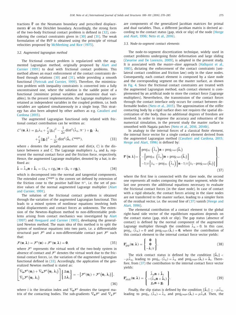
moothed with Nagata patches ( Neto et al., 2016, 2014b) . In analogy to the internal forces of a classical finite element,

he internal force vector for a single contact element derived fromhe augmented Lagrangian method ( Cavalieri and Cardona, 2015;eege and Alart, 1996) is defined by:

c (u , λ

)=

⎧ ⎪ ⎪ ⎪ ⎨ ⎪ ⎪ ⎪ ⎩

pro j R

−

(ˆ λn

)n + pro j C augm

( λt

)−{

pro j R

−

(ˆ λn

)n + pro j C augm

( λt

)} −1 /ε

{ λn − pro j R

−

(ˆ λn

)} n −1 /ε

{λt −pro j C augm

( λt

)}⎫ ⎪ ⎪ ⎪ ⎬ ⎪ ⎪ ⎪ ⎭

,

(37)

here the first line is connected with the slave node, the second

ne represents all nodes composing the master segment, while the

ast one presents the additional equations necessary to evaluate

he frictional contact forces (in the slave node). In case of contact

ith a rigid obstacle, the contact forces arising in the slave nodes

re not transferred to the master surface, leading to a simpler form

f the residual vector, i.e. the second line of ( 37 ) vanish ( Heege and

lart, 1996 ).

The elemental contribution of a contact element to the global

ight-hand side vector of the equilibrium equations depends on

he contact status (gap, stick or slip). The gap status (absence of

ontact) is defined by the normal component of the augmented

agrange multiplier through the condition

ˆ λn > 0 . In this case,

ro j � − ( λn ) = 0 and pro j C augm ( λt ) = 0 , where the contribution of

his contact element to the internal contact force vector yields:

c gap (u , λ) =

{

0

0

−λ/ε

}

. (38)

The stick contact status is defined by the condition ‖ λt ‖ <μˆ λn , leading to pro j � − ( λn ) =

λn and pro j C augm ( λt ) =

λt . There-

ore, from ( 37 ) the contribution to the internal contact force vector

ields:

c stick (u , λ) =

⎧ ⎨ ⎩

ˆ λn n +

λt

−( λn n +

λt ) g n n + g t

⎫ ⎬ ⎭

. (39)

Finally, the slip status is defined by the condition ‖ λt ‖ ≥ −μˆ λn ,

eading to pro j − ( λn ) =

λn and pro j augm ( λt ) = μˆ λn t . Then, the


Fig. 4. Graphical representation of the node-to-segment contact discretization considering the master body: (a) rigid; (b) deformable.

Table 3

Main dimensions of the forming tools for both stages

(mm) ( Gelin and Picart, 1999 ).

Tool geometry Stage 1 Stage 2

Die opening diameter 104 .5 78 .0

Die radius 8 .0 5 .5

Die height 21 .0 16 .0

Punch diameter 100 .0 73 .4

Punch radius 5 .5 8 .5

Blank-holder opening diameter 104 .5 105 .0

Blank-holder radius – 7 .0

Blank-holder height 10 .0 30 .0

i

p

w

u

(

t

i

a

i

3

d

a

p

d

s

w

o

n

m

t

r

F

o

e

a

m

i

4

s

s

p

t

h

n

o

p

i

f

contribution of this contact element to the internal contact force

vector is given by:

F c slip (u , λ) =

⎧ ⎨ ⎩

ˆ λn (n − μt )

−( λn (n − μt ))

g n n − ( λt + μˆ λn t ) /ε

⎫ ⎬ ⎭

, (40)

where the tangential slip direction unit vector is defined by:

t =

ˆ λt / ‖

λt ‖ . (41)

The Jacobian matrices associated to the internal force vector

( 37 ) were derived by Neto et al. (2016 ) for each contact status

(gap, stick or slip). The pattern of nonzero entries in the global

tangent matrix is symmetric. Nevertheless, the pattern needs to be

update in large sliding contact problems, which is computationally

expensive. On the other hand, the global tangent matrix presents a

fixed pattern when the master surface is assumed rigid ( Neto et al.,

2015 ).

4. Reverse deep drawing

In order to accomplish high drawing ratios in the deep draw-

ing process, it is usually decomposed into several forming stages.

The reverse deep drawing of a cylindrical cup, proposed at the

Numisheet’99 conference, is the forming process selected in this

study ( Gelin and Picart, 1999 ). This deep drawing process is char-

acterized by the change of the drawing direction from the first to

the second stage, i.e. the punch travels in the reverse direction dur-

ing the second stage. The deep drawing quality (DDQ) mild steel is

the material selected for the blank, which has 170 mm of initial

diameter and 0.98 mm in thickness.

4.1. Experimental setup

The experimental drawing device was developed by Thuillier

et al. (2002 ) in order to be attached at the connecting ends of

a classical tensile test machine. The apparatus of the first stage

is composed by a hollow punch of 100 mm external diameter, a

die with an internal diameter of 104.5 mm and a blank-holder

(see Fig. 5 (a)). In order to impose a fixed initial gap between the

blank-holder and the die, the tools are connected by means of

eight screws and adjustable washers put in-between, as shown in

Fig. 5 (a). An identical procedure is adopted in the second stage,

where the blank-holder is connected to the die by means of a hat-

shaped part, as shown in Fig. 5 (b). Note that the punch of the first

stage becomes the die of the second forming stage, as highlighted

in Fig. 5 . The main dimensions of the forming tools are given in

Table 3.

The punch involved in each forming stage was built in hard-

ened tool steel while the other tools and connection parts were

made of high strength steel. All surfaces of the forming tools with

the possibility to establish contact with the blank are heat treated

and ground to obtain a high value of hardness ( Thuillier et al.,

2010 ). The gap between the die and the blank-holder was held

fixed in both stages by means of a pile of adjustable washers put

n-between. The total height of these washers was determined ex-

erimentally as large as possible in order to draw a cylindrical cup

ithout wrinkles. For the studied material, the measured gap val-

es are 1.0 mm for the first stage and 1.4 mm for the second stage

Thuillier et al., 2002 ). The blank is lubricated on both sides at

he beginning of the process, as well as before the second form-

ng stage, reducing the friction forces arising between the blank

nd the forming tools. The depth of the cylindrical cups is 50 mm

n the first stage and 70 mm in the second stage.

The punch speed during the forming operation (both stages) is

.3 mm/s. The accuracy reached in the measurement of the punch

isplacement is ± 0.02 mm, while the load is recorded with 0.4% of

ccuracy ( Thuillier et al., 2010 ). Five forming tests under identical

rocess conditions were performed in order to check the repro-

ucibility of the obtained experimental data. After the first stage,

ome cylindrical cups are extracted for thickness measurement,

hile others are deformed in the reverse direction. The thickness

f the cup wall is measured using a three-dimensional coordi-

ate measuring machine (DEA Swift A001). Three straight lines are

arked on the sheet before forming (0 º, 45 º and 90 º) to perform

he thickness measurement in three directions to the rolling di-

ection, using an increment of 1 mm between consecutive points.

urthermore, a hole is trimmed in the bottom of the cup to fix it

n the table of the measuring machine. The point coordinates are

valuated on both sides of the cylindrical cups (inside and outside)

t the same height, allowing the definition of a horizontal distance

easured in the radial direction ( Thuillier et al., 2010 ), as shown

n Fig. 6.

.2. Finite element model

The numerical simulations were carried out with the in-house

tatic implicit finite element code DD3IMP ( Menezes and Teodo-

iu, 20 0 0 ), specifically developed to simulate sheet metal forming

rocesses ( Oliveira et al., 2008 ). In order to improve the computa-

ional performance, some high-performance computing techniques

ave been incorporated to take advantage of multi-core processors,

amely OpenMP directives in the most time-consuming branches

f the code ( Menezes et al., 2011 ). All numerical simulations were

erformed on a computer machine equipped with an Intel ® Core TM

7–4770 K Quad-Core processor (3.5 GHz) and the Windows 7 Pro-

essional (64-bit platform) operating system.


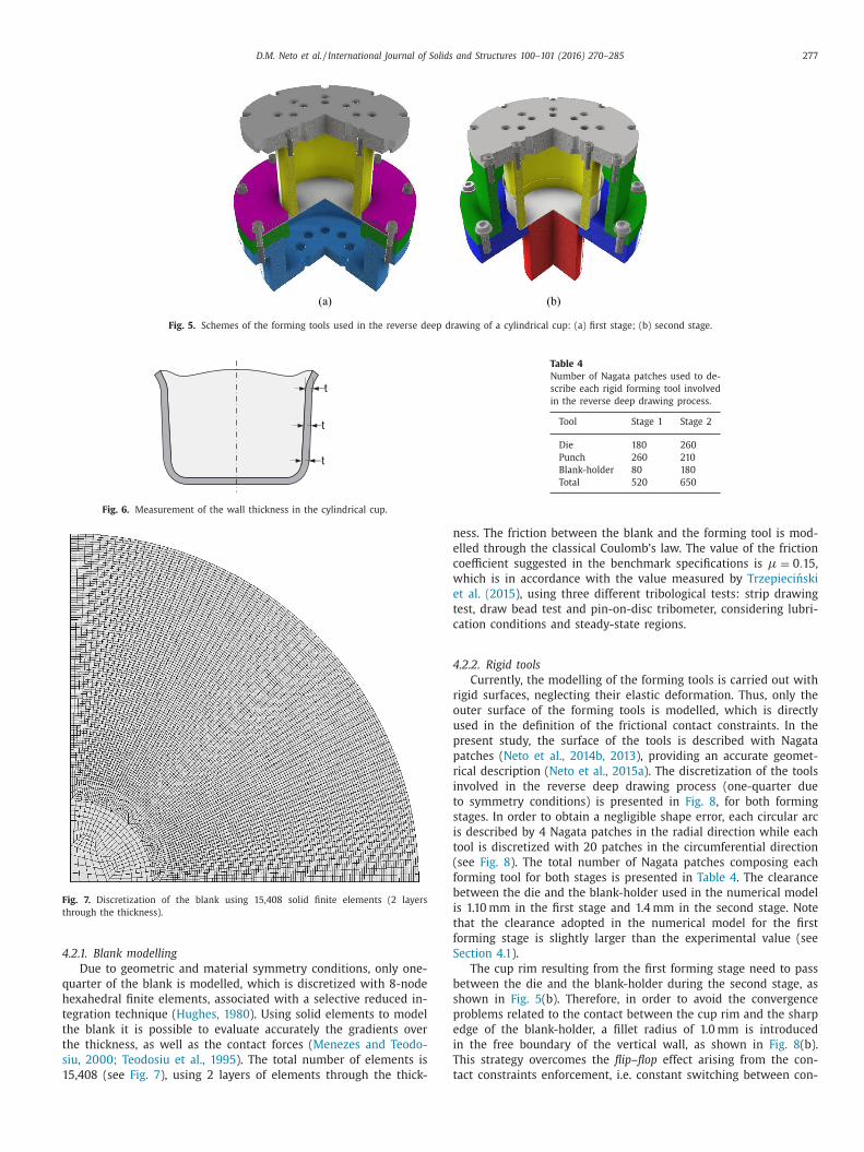
Fig. 5. Schemes of the forming tools used in the reverse deep drawing of a cylindrical cup: (a) first stage; (b) second stage.

t

t

t

Fig. 6. Measurement of the wall thickness in the cylindrical cup.

Fig. 7. Discretization of the blank using 15,408 solid finite elements (2 layers

through the thickness).

4

q

h

t

t

t

s

1

Table 4

Number of Nagata patches used to de-

scribe each rigid forming tool involved

in the reverse deep drawing process.

Tool Stage 1 Stage 2

Die 180 260

Punch 260 210

Blank-holder 80 180

Total 520 650

n

e

c

w

e

t

c

4

r

o

u

p

p

r

i

t

s

i

t

(

f

b

i

t

f

S

b

s

p

e

i

T

t

.2.1. Blank modelling

Due to geometric and material symmetry conditions, only one-

uarter of the blank is modelled, which is discretized with 8-node

exahedral finite elements, associated with a selective reduced in-

egration technique ( Hughes, 1980 ). Using solid elements to model

he blank it is possible to evaluate accurately the gradients over

he thickness, as well as the contact forces ( Menezes and Teodo-

iu, 20 0 0; Teodosiu et al., 1995 ). The total number of elements is

5,408 (see Fig. 7 ), using 2 layers of elements through the thick-

ess. The friction between the blank and the forming tool is mod-

lled through the classical Coulomb’s law. The value of the friction

oefficient suggested in the benchmark specifications is μ = 0 . 15 ,

hich is in accordance with the value measured by Trzepieci nski

t al. (2015 ), using three different tribological tests: strip drawing

est, draw bead test and pin-on-disc tribometer, considering lubri-

ation conditions and steady-state regions.

.2.2. Rigid tools

Currently, the modelling of the forming tools is carried out with

igid surfaces, neglecting their elastic deformation. Thus, only the

uter surface of the forming tools is modelled, which is directly

sed in the definition of the frictional contact constraints. In the

resent study, the surface of the tools is described with Nagata

atches ( Neto et al., 2014b, 2013 ), providing an accurate geomet-

ical description ( Neto et al., 2015a ). The discretization of the tools

nvolved in the reverse deep drawing process (one-quarter due

o symmetry conditions) is presented in Fig. 8 , for both forming

tages. In order to obtain a negligible shape error, each circular arc

s described by 4 Nagata patches in the radial direction while each

ool is discretized with 20 patches in the circumferential direction

see Fig. 8 ). The total number of Nagata patches composing each

orming tool for both stages is presented in Table 4 . The clearance

etween the die and the blank-holder used in the numerical model

s 1.10 mm in the first stage and 1.4 mm in the second stage. Note

hat the clearance adopted in the numerical model for the first

orming stage is slightly larger than the experimental value (see

ection 4.1 ).

The cup rim resulting from the first forming stage need to pass

etween the die and the blank-holder during the second stage, as

hown in Fig. 5 (b). Therefore, in order to avoid the convergence

roblems related to the contact between the cup rim and the sharp

dge of the blank-holder, a fillet radius of 1.0 mm is introduced

n the free boundary of the vertical wall, as shown in Fig. 8 (b).

his strategy overcomes the flip –flop effect arising from the con-

act constraints enforcement, i.e. constant switching between con-


Die

Punch

Blank-holder

Blank

xyz

Die

Blank

Punch

Blank-holder

Fig. 8. Discretization of the (rigid) forming tools using Nagata patches: (a) first stage; (b) second stage.

Fig. 9. Discretization of the (deformable) forming tools using solid finite elements: (a) first stage; (b) second stage.

Table 5

Number of finite elements used to de-

scribe each deformable forming tool

involved in the reverse deep drawing

process.

Tool Stage 1 Stage 2

Die 2480 2880

Punch 2880 3003

Blank-holder 480 1320

Total 5840 7203

N

s

fi

s

r

d

t

a

w

a

tact and gap statuses ( Neto et al., 2015 ). An identical procedure is

adopted in the model that considers deformable tools.

4.2.3. Deformable tools

Due to geometric and material symmetry conditions, only one-

quarter of the forming tools is modelled. They are discretized with

solid finite elements, allowing take into account its elastic defor-

mation. Typically, the surface details involved in the tools require

a fine mesh in these zones, leading to a significant increase in the

total number of finite elements. This issue can be overcome by ap-

plying a surface smoothing method on the coarse mesh, provid-

ing an accurate description of the curved surfaces using a small

amount of finite elements. Several surface smoothing procedures

have been proposed in the last decade ( Neto et al., 2015 ). In the

present study, each tool surface is smoothed with Nagata patches,

following the procedure proposed by Neto et al. (2016 ) for fric-

tional contact problems between deformable bodies.

The discretization of each forming tool involved in the reverse

deep drawing process is presented in Fig. 9 . The discretization of

the deformable tools in the curved surfaces is identical to the pre-

viously used for rigid tools (compare Fig. 8 and Fig. 9 ), providing

a similar shape error resulting from the surface interpolation with

agata patches. Consequently, the geometrical accuracy of the tool

urfaces is the same for both finite element models. The number of

nite elements used to define each deformable forming tool is pre-

ented in Table 5 . The geometry of the tools was simplified in the

egion of the screws (see Fig. 5 ), where adequate boundary con-

itions are applied to represent the physical connection between

he die and the blank-holder. Since the screws are located on a di-

meter of 185 mm (see Section 4.1 ), the tools are modelled only

ithin this perimeter, which is fixed in all directions, establishing

n initial clearance of 1.0 mm between them. Besides, the vertical


0

10

20

30

40

50

60

70

80

90

0 10 20 30 40 50

]Nk[ ecrof hcnuP

Punch displacement [mm]

Experimental [Thuillier 2002]

Rigid tools (gap=1.10 mm)

Deformable tools

Fig. 10. Comparison between experimental and numerical punch force evolution

during the first forming stage.

d

A

s

t

t

b

N

4

4

m

c

T

e

4

f

G

m

t

i

b

m

i

i

t

c

t

t

H

t

t

p

f

t

m

f

m

c

a

p

p

f

l

w

w

i

T

t

r

m

b

t

f

(

i

p

t

e

t

e

d

t

t

f

i

v

c

a

t

a

t

u

a

s

t

p

s

i

t

t

a

e

t

m

fl

m

s

a

b

e

f

o

4

s

u

p

(

f

c

t

isplacement imposed to the punch is applied on its top surface.

ccordingly, an identical procedure is adopted for the tools of the

econd stage.

The mechanical behaviour of the forming tools is assumed elas-

ic and isotropic (von Mises). Since the tools are made of steel,

heir elastic properties are identical to the ones adopted for the

lank, i.e. Young’s modulus of 210 GPa and Poisson ratio of 0.30.

evertheless, their yield strength is significantly higher, about

00 MPa.

.3. Results and discussion

The comparison between different numerical approaches to

odel the forming tools is presented. Furthermore, the numeri-

al results are compared with the experimental ones provided by

huillier et al. (2002 ), highlighting the influence of the tools mod-

lling in the accuracy of the finite element solution.

.3.1. Forming forces

The comparison between experimental and numerical punch

orce evolution is shown in Fig. 10 , for the first forming stage.

lobally, the experimental punch force is overestimated by the nu-

erical model that takes into account the elastic deformation of

he tools, while it is underestimated when considering rigid tools

n the finite element model. Nevertheless, note that the clearance

etween the die and the blank-holder adopted in the finite ele-

ent model using rigid tools (1.10 mm) is higher than the exper-

mental value (1.0 mm). Since the deformation mode of the sheet

s close to uniaxial compression in the flange ( Neto et al., 2014a ),

he increase of the sheet thickness in this region leads to an in-

rease of punch force due to the large restraining forces. Therefore,

he clearance between the die and the blank-holder was enlarged

o avoid the ironing of the flange in the finite element simulation.

owever, the adopted value of clearance (1.10 mm) is not sufficient

o completely eliminate the ironing effect, which is highlighted by

he abrupt increase of the punch force at approximately 35 mm of

unch displacement (see Fig. 10 ). On the other hand, the punch

orce evolution provided by the numerical model using deformable

ools (1.0 mm of initial gap) is in better agreement with the experi-

ental one, as shown in Fig. 10 . The sudden decrease of the punch

orce at around 43 mm of displacement occurs for both numerical

odels (rigid and deformable tools), which is related to the loss of

ontact between the sheet and the blank-holder. The possible mis-

lignment of the sheet with the forming tools in the experimental

rocedure may explain the smoother decrease of the experimental

unch force.

Although the mesh adopted in the discretization of the de-

ormable forming tools ( Fig. 9 ) can be considered coarse, the evo-

ution of the punch force is smooth (see Fig. 10 ). This is related

ith the applied surface smoothing procedure ( Neto et al., 2016 ),

hich eliminates the nonphysical oscillations in the contact force

nduced by the discontinuity of the surface normal vector field.

he nodal contact forces arising in the slave nodes belonging to

he symmetry plane are presented in Fig. 11 , for the instant cor-

esponding to 25 mm of punch displacement. The contact occurs

ainly in the curved zones of the forming tools, where it is possi-

le to see that the surface smoothing method is effective. In fact,

he contact forces are properly distributed on the smoothed sur-

ace, despite the apparent gap between the punch and the sheet

see Fig. 11 (a)) and between the die and the sheet (see Fig. 11 (b)),

n the curved contact zones.

Concerning the second forming stage, Fig. 12 presents the com-

arison between experimental and numerical punch force evolu-

ion. The numerical results are similar for both finite element mod-

ls (rigid and deformable tools), indicating that the tools deforma-

ion is negligible in the second stage. The numerical punch force

volution is in very good agreement with the experimental one

uring the initial 35 mm of punch displacement. In fact, the ini-

ial slope predicted by the numerical simulation is coincident with

he experimental one. On the other hand, the experimental punch

orce exhibits a peak for a punch stroke around 40 mm, which

s underestimated by the numerical simulation, both in terms of

alue and the instant of occurrence, as shown in Fig. 12 . Since the

ylindrical cup is not completely formed, this peak of the force is

ssociated with the passage of the cup rim between the die and

he blank-holder (see Fig. 9 (b)). The difference between numerical

nd experimental force peak is connected with the final value of

he punch force in the first forming stage (see Fig. 10 ), which is

nderestimated by the numerical simulation. Thus, the slight mis-

lignment of the sheet with the forming tools in the experimental

etup can lead to an increase of the restraining forces arising in

he cup rim.

The evolution of the blank-holder force as a function of the

unch displacement is presented in Fig. 13 , for both forming

tages, comparing the two numerical models developed. Regard-

ng the first stage, the force value predicted by the model that

akes into account the tools deformation is globally higher than

he one obtained considering rigid tools. Note that the fixed clear-

nce between the die and the blank-holder is larger in the finite

lement model using rigid tools (1.10 mm). The abrupt increase of

he blank-holder force at approximately 35 mm of punch displace-

ent (see Fig. 13 ) is a consequence of the ironing effect in the

ange, which only occurs when using rigid tools in the finite ele-

ent model. The magnitude of the blank-holder force during the

econd forming stage is considerably lower than in the first stage,

s shown in Fig. 13 , since the clearance between the die and the

lank-holder is larger (see Section 2 ). Moreover, the small differ-

nce between the two finite element models in terms of predicted

orces indicates an insignificant deflection of the tools in the sec-

nd stage.

.3.2. Tools deflection

The deflection of the tools during the first forming stage is as-

essed in the present study through the nodal displacements eval-

ated in the tools, specifically the blank-holder and the die. Fig. 14

resents the evolution of the vertical displacement of six nodes

three positioned in the blank-holder and three in the die) as a

unction of the punch displacement. The deformation of the tools

omes up from the thickening of the flange, which is induced by

he circumferential compressive stress state (uniaxial compressive


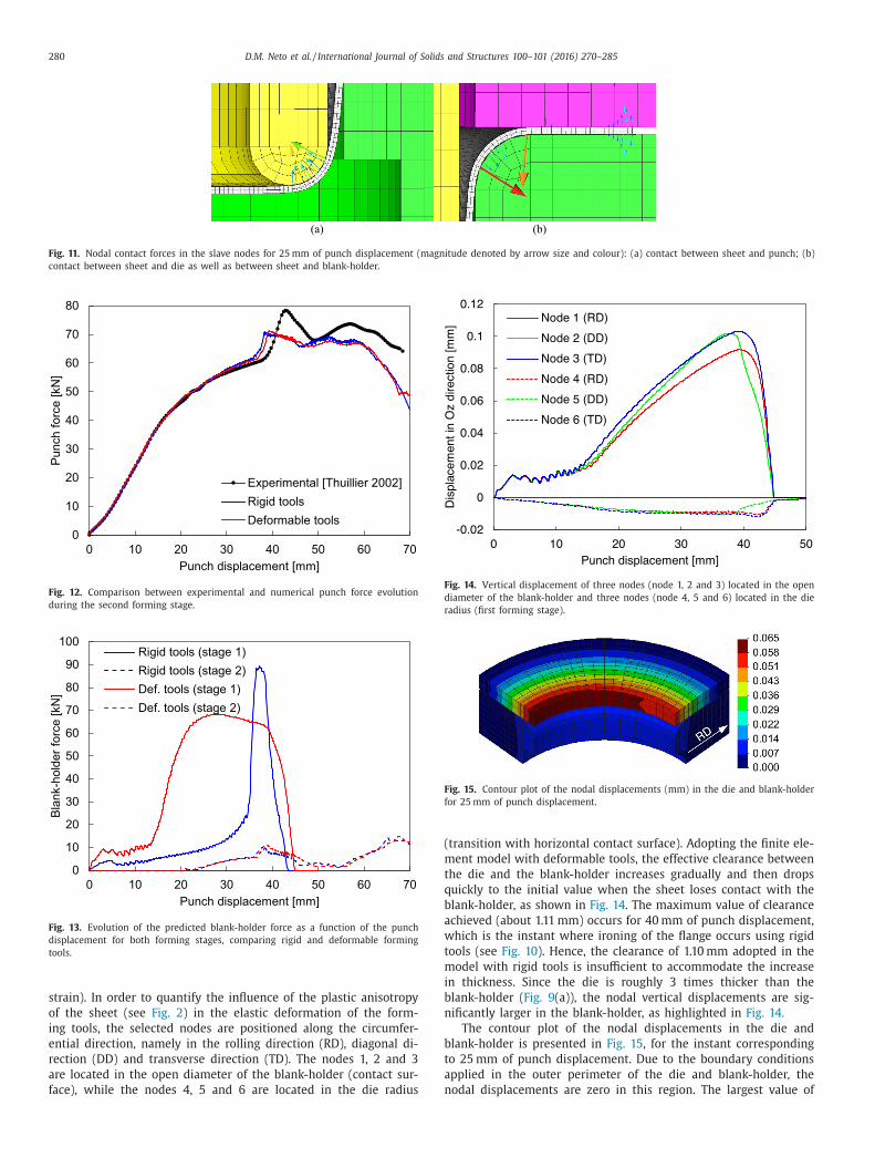
Fig. 11. Nodal contact forces in the slave nodes for 25 mm of punch displacement (magnitude denoted by arrow size and colour): (a) contact between sheet and punch; (b)

contact between sheet and die as well as between sheet and blank-holder.

0

10

20

30

40

50

60

70

80

0 10 20 30 40 50 60 70

]Nk[ ecrof hcnuP


Experimental [Thuillier 2002]Rigid toolsDeformable tools

Fig. 12. Comparison between experimental and numerical punch force evolution

during the second forming stage.

0

10

20

30

40

50

60

70

80

90

100

0 10 20 30 40 50 60 70

knalB

-]

Nk[ ec rof redlo h


Rigid tools (stage 1)Rigid tools (stage 2)Def. tools (stage 1)Def. tools (stage 2)

Fig. 13. Evolution of the predicted blank-holder force as a function of the punch

displacement for both forming stages, comparing rigid and deformable forming

tools.

Fig. 14. Vertical displacement of three nodes (node 1, 2 and 3) located in the open

diameter of the blank-holder and three nodes (node 4, 5 and 6) located in the die

radius (first forming stage).

Fig. 15. Contour plot of the nodal displacements (mm) in the die and blank-holder

for 25 mm of punch displacement.

(

m

t

q

b

a

w

t

m

i

b

n

b

t

a

n

strain). In order to quantify the influence of the plastic anisotropy

of the sheet (see Fig. 2 ) in the elastic deformation of the form-

ing tools, the selected nodes are positioned along the circumfer-

ential direction, namely in the rolling direction (RD), diagonal di-

rection (DD) and transverse direction (TD). The nodes 1, 2 and 3

are located in the open diameter of the blank-holder (contact sur-

face), while the nodes 4, 5 and 6 are located in the die radius

transition with horizontal contact surface). Adopting the finite ele-

ent model with deformable tools, the effective clearance between

he die and the blank-holder increases gradually and then drops

uickly to the initial value when the sheet loses contact with the

lank-holder, as shown in Fig. 14 . The maximum value of clearance

chieved (about 1.11 mm) occurs for 40 mm of punch displacement,

hich is the instant where ironing of the flange occurs using rigid

ools (see Fig. 10 ). Hence, the clearance of 1.10 mm adopted in the

odel with rigid tools is insufficient to accommodate the increase

n thickness. Since the die is roughly 3 times thicker than the

lank-holder ( Fig. 9 (a)), the nodal vertical displacements are sig-

ificantly larger in the blank-holder, as highlighted in Fig. 14.

The contour plot of the nodal displacements in the die and

lank-holder is presented in Fig. 15 , for the instant corresponding

o 25 mm of punch displacement. Due to the boundary conditions

pplied in the outer perimeter of the die and blank-holder, the

odal displacements are zero in this region. The largest value of


1

1.01

1.02

1.03

1.04

1.05

1.06

1.07

50 55 60 65 70 75 80 85 90

]m

m[ etanid rooc z

Radial coordinate [mm]

RDDDTD

Fig. 16. Profile of the blank-holder surface (first forming stage) measured in three

directions, for 25 mm of punch displacement.

Fig. 17. von Mises stress distribution (MPa) in the forming tools for 25 mm of

punch displacement.

d

i

t

t

v

(

fi

s

t

t

D

f

t

t

fl

t

i

t

T

t

f

b

r

o

t

s

S

m

Rigidtools

Deformabletools

RD

Fig. 18. Equivalent plastic strain distribution plotted in the deformed configuration

of the cylindrical cup after the first forming stage. Finite element model using rigid

tools (left) and using deformable tools (right).

Fig. 19. Experimental geometry of the cylindrical cup obtained by reverse deep

drawing: (a) first stage; (b) second stage.

e

d

b

t

o

t

4

f

t

i

d

F

m

e

t

n

t

i

s

d

o

h

f

e

c

c

c

a

isplacement occurs in the blank-holder opening diameter, which

s predominantly in the vertical direction. On the other hand, for

he same radial distance, the deflection of the die is at least 5

imes lower than the one of blank-holder. Indeed, the maximum

alue of the nodal displacements is inferior to 0.014 mm in the die

see Fig. 15 ).

The deformed configuration of the blank-holder involved in the

rst forming stage is presented in Fig. 16 , for the instant corre-

ponding to 25 mm of punch displacement. In order to analyse

he influence of the sheet anisotropy in the blank-holder deflec-

ion, three different cross sections are assessed, namely in the RD,

D and TD. The profile of the deformed blank-holder is different

or each analysed cross section (see Fig. 16 ), because the predicted

hickness distribution is non-uniform in the circumferential direc-

ion and the draw-in is asymmetric. Indeed, the thickness of the

ange and its draw-in are directly connected through the assump-

ion of the incompressibility condition ( Neto et al., 2014a ), present-

ng opposite effects on the blank-holder deflection. Accordingly,

he clearance between the die and the blank-holder is larger in the

D and smaller in the RD, as shown in Fig. 16 . However, the rela-

ive trend between the three sections presents changes during the

orming process evolution, specifically in the DD (see Fig. 14 ).

The von Mises stress distribution in the forming tools (punch,

lank-holder and die) is presented in Fig. 17 , for the instant cor-

esponding to 25 mm of punch displacement. The maximum value

f the stress arises close to the perimeter of the blank-holder due

o the applied boundary conditions (prescribed displacements) and

mall stiffness of the blank-holder in comparison with the die.

ince the maximum value of equivalent stress predicted by the nu-

erical simulation is about 112 MPa, the forming tools only exhibit

lastic deformation during the cup forming. Additionally, the stress

istribution is asymmetric in the tools ( Fig. 17 ), which is induced

y the plastic anisotropy of the sheet. Nevertheless, the stress dis-

ribution in the punch is less influenced by the plastic anisotropy

f the sheet, since the contact zone is almost insensitive to sheet

hickness variations.

.3.3. Cup geometry

The significant deflection of the blank-holder during the first

orming stage affects the material flow, as the distribution of con-

act pressure on the flange is different from the one obtained us-

ng rigid tools ( Shulkin et al., 1996 ). The equivalent plastic strain

istribution predicted by finite element simulation is presented in

ig. 18 , at the end of the first forming stage, comparing the nu-

erical models analysed (rigid and deformable tools). Although the

lastic deformation of the blank-holder is non-negligible ( Fig. 15 ),

he final configuration of the cylindrical cup is identical for both

umerical models. Since the punch force is nonzero at the end of

he first stage (see Fig. 10 ), the cup is not fully drawn, as shown

n the experimental geometry of the cup after the first stage pre-

ented in Fig. 19 (a). The maximum value of plastic strain pre-

icted by the numerical model is reached in the cup rim. The value

f equivalent plastic strain is lower in the DD for the same cup

eight, which is in accordance with the earing profile (four ears).

The final configuration of the cylindrical cup after the second

orming stage is presented in Fig. 20 , comparing the two finite

lement models proposed in Section 3 . The main difference oc-

urs in the DD, where the numerical model that takes into ac-

ount the elastic deformation of the forming tools predicts the oc-

urrence of wrinkling. The large circumferential compressive stress

nd the earing effect induced by the plastic anisotropy yields the


Rigidtools

Deformabletools

RD

Fig. 20. Equivalent plastic strain distribution plotted in the deformed configuration

of the cylindrical cup after the second forming stage. Finite element model using

rigid tools (left) and using deformable tools (right).

Fig. 21. Experimental and numerical thickness distributions in the cup wall after

the first forming stage at: (a) RD; (b) DD; (c) TD.

c

a

d

d

s

T

r

t

o

T

t

i

wrinkling defect, when the flange loses contact with the blank-

holder. In fact, the amplitude of the ears at the end of the first

forming stage is larger when considering the elastic deformation of

the forming tools, because the effective clearance between the die

and the blank-holder is smaller and, consequently, the restraining

forces are higher (see Fig. 13 ). The equivalent plastic strain distri-

bution predicted by numerical simulation is shown in Fig. 20 , com-

paring both numerical models. The maximum value occurs in the

cup rim, specifically in the region of wrinkling. The predicted plas-

tic strain distribution is similar for both numerical models, except

in the wrinkling region. Since the plastic strain increases in the

second forming stage, the amplitude of the four ears is enlarged

from the first to the second drawing stage (compare Fig. 18 with

Fig. 20 ), which is in accordance with the experimental observations

(see Fig. 19 ). The slight misalignment of the sheet with the forming

tools in the experimental procedure is confirmed by the asymme-

try in the rim of the cylindrical cup, shown in Fig. 19 (b).

4.3.4. Thickness distribution

The comparison between experimental and numerical thickness

distribution in the cup wall after the first forming stage is shown

in Fig. 21 , for three different directions (RD, DD and TD). The nu-

merical thickness is evaluated in the radial direction (see Fig. 6 ) ac-

cording to the experimental procedure. Globally, the thickness dis-

tribution predicted by the numerical model that takes into account

the elastic deformation of the forming tools is in very good agree-

ment with the experimental evolution, as shown in Fig. 21 . On the

other hand, the cup thickness is clearly overestimated when the

forming tools are assumed as rigid.

Since the effective clearance between the die and the blank-

holder is lower when the deformation of the forming tools is

taken into account (model with rigid tools presents a fixed value

of 1.10 mm), the restraining forces arising in the flange are glob-

ally higher (see Fig. 13 ). Thus, the predicted cup wall thickness is

lower and the height of the cylindrical cup is slightly higher us-

ing the finite element model with deformable tools. This differ-

ence in the cup height delays the instant in which the punch force

increases abruptly during the second forming stage (see Fig. 12 ),

which is associated with the passage of the cup rim between the

die and the blank-holder. Due to the plastic anisotropy of the sheet

( Fig. 2 ), the cup wall is thicker in the DD (see Fig. 21 ), which is

in accordance with the earing profile presented in Fig. 18 . The as-

sumption of rigid tools leads to an unexpected decrease of the pre-

dicted thickness in the TD for 28 mm of cup height (see Fig. 21 (c)),

which is associated with the flange ironing, i.e. the abrupt increase

of the blank-holder force shown in Fig. 13 . The ironing effect oc-

urs mainly in this direction since the anisotropic behaviour yields

sheet thickening higher in TD, as highlighted in the blank-holder

eflection shown in Fig. 16.

The comparison between experimental and numerical thickness

istribution in the cup wall after the second forming stage is pre-

ented in Fig. 22 , for three different directions (RD, DD and TD).

he experimental thickness distribution is overestimated in all di-

ections by both numerical models. Nevertheless, the accuracy of

he finite element model that takes into account the deformation

f the forming tools is better than the one assuming rigid tools.

his improvement results mainly from the numerical thickness dis-

ribution achieved for the first forming stage (see Fig. 21 ), which

s in very good agreement with the experimental measurement,


Fig. 22. Experimental and numerical thickness distributions in the cup wall after

the second forming stage at: (a) RD; (b) DD; (c) TD.

w

t

f

s

m

F

c

t

r

s

i

t

Table 6

Computational performance of both finite element models used in the reverse deep

drawing simulation.

Stage 1 Stage 2

Rigid tools Deformable tools Rigid tools Deformable tools

N º increments 928 2641 761 1637

Average n ºiterations

6 .65 7 .50 6 .95 8 .58

Computational

time [h]

1 .37 18 .88 1 .13 10 .48

m

l

i

l

4

m

m

i

e

t

m

t

c

r

s

q

d

u

i

m

n

d

t

q

a

i

s

5

d

T

a

c

d

t

a

a

p

s

s

t

t

p

t

c

t

l

t

hen the tools deformation is considered. Indeed, the slope of the

hickness distribution predicted by the numerical model with de-

ormable tools is in good agreement with the experimental one,

pecifically in the RD and TD. On the other hand, this finite ele-

ent model predicts the occurrence of wrinkling in the DD (see

ig. 20 ), which overestimate considerably the wall thickness for a

up height superior to 55 mm, as shown in Fig. 22 (b).

The thickness predicted by finite element simulation is higher

han the one measured experimentally because the value of the

estraining forces arising in the cup rim during the second forming

tage (40 mm of punch displacement) is underestimated, as shown

n Fig. 12 . Since the thickness of the cup wall is overestimated by

he finite element simulation ( Fig. 22 ), the cup height is underesti-

ated. Consequently, for the same punch displacement, the small

ength of the flange located between the die and the blank-holder

nduces a delay of the punch force evolution after its peak, as high-

ighted in Fig. 12.

.3.5. Computational performance

The computational performance of the proposed finite element

odels is presented in Table 6 . The adoption of the numerical

odel that takes into account the elastic deformation of the form-

ng tools leads to an increase in the number of increments, the av-

rage number of iterations and the computational time. Although

he significant improvements achieved in the accuracy of the nu-

erical results (punch force evolution and thickness distribution),

he computational cost increases considerably, as shown in Table 6.

Regarding the first forming stage, the computational time in-

reases roughly 14 times in comparison with the model that uses

igid tools, while it increases approximately 9 times in the second

tage. Indeed, the increase of the computational cost is a conse-

uence of several factors: (i) higher number of DOF due to the

iscretization of the tools with solid elements (see Table 5 ); (ii)

pdate the nonzero pattern of the global tangent matrix in each

ncrement due to large sliding ( Neto et al., 2016 ); (iii) small incre-

ent size required to avoid convergence problems and (iv) higher

umber of iterations per increment. Since the contact between a

eformable body and a rigid surface is a particular case of the con-

act between two deformable bodies, the number of increments re-

uired in each forming stage increases when the forming tools are

ssumed deformable. In fact, the number of increments is approx-

mately 3 times higher in the first stage and about 2 times in the

econd forming stage.

. Conclusions

The elastic deformation of the forming tools during the reverse

eep drawing of a cylindrical cup is evaluated in the present paper.

he blank-holder and the die are connected by means of screws

nd adjustable washers put in-between, establishing a fixed initial

learance between them. Two distinct finite element models are

eveloped to quantify the influence of the tools deformation on

he material flow, i.e. the forming tools are assumed perfectly rigid

s well as deformable. Moreover, the obtained numerical results

re compared with the experimental measurements to validate the

roposed finite element model.

The distribution of the contact pressure in the flange and, con-

equently, the material flow are strongly influenced by the as-

umptions adopted in the numerical model concerning the forming

ools. The elastic deflection of the blank-holder is a consequence of

he sheet thickening, which is induced by the circumferential com-

ressive stress arising in the flange. Therefore, taking into account

he deformation of the tools in the numerical model, the effective

learance between the die and the blank-holder increases during

he forming process, while the restraining forces in the flange are

ower. Indeed, the predicted clearance increases about 10% during

he first forming stage, while the deflection of the tools is negligi-


D

F

G

G

G

G

H

H

H

H

H

H

H

H

H

K

L

M

M

M

M

M

M

M

N

ble in the second stage. Accordingly, the experimental punch force

of the first forming stage is slightly overestimated by this numeri-

cal model, while the assumption of rigid tools leads to the ironing

effect in the flange. Besides, considering the elastic deformation of

the forming tools, the predicted thickness distribution in the cup

wall is in very good agreement with the experimental measure-

ments. Nevertheless, the computational cost is significantly higher

in comparison with the classic model using rigid tools.

Therefore, the accuracy of the sheet metal forming simulation

can be improved considering the elastic deformation of the form-

ing tools in the numerical model. This is particularly important in

forming processes of high strength steels and reduced structural

stiffness of the tools, where the deflection of the tools is sub-

stantial. However, the computational time increases considerably

in comparison with the assumption of rigid tools. Thus, the nu-

merical model that takes into account the elastic deformation of

the forming tools should be adopted only in specific cases.

Acknowledgements

The authors gratefully acknowledge the financial support of

the Portuguese Foundation for Science and Technology (FCT)

under projects with reference UID/EMS/00285/2013, P2020-

PTDC/EMS-TEC/0702/2014 (POCI-01-0145-FEDER-016779) and

P2020-PTDC/EMS-TEC/6400/2014 (POCI-01-0145-FEDER-016876)

by UE/FEDER through the program COMPETE2020. The first

author is also grateful to the FCT for the Postdoctoral grant

SFRH/BPD/101334/2014.

References

Alart, P., Curnier, A., 1991. A mixed formulation for frictional contact problems proneto Newton like solution methods. Comput. Methods Appl. Mech. Eng. 92, 353–

375. doi: 10.1016/0 045-7825(91)90 022-X .

Alart, P.P., 1997. Méthode de Newton généralisée en mécanique du contact. J. Math.Pures Appl. 76, 83–108. doi: 10.1016/S0021- 7824(97)89946- 1 .

Alves, J.L. , 2003. Simulação Numérica do Processo de Estampagem de ChapasMetálicas: Modelação Mecânica e Métodos Numéricos. University of Minho .

Alves, J.L., Bouvier, S., Joma a, M., Billardon, R., Oliveira, M.C., Menezes, L.F., 2007.Kinematic hardening: characterization, modeling and impact on springback pre-

diction. AIP Conf. Proc. 908, 691–698. doi: 10.1063/1.2740891 .

Belytschko, T. , Liu, W.K. , Moran, B. , 20 0 0. Nonlinear Finite Elements for Continuaand Structures. John Wiley & Sons .

Cavalieri, F.J., Cardona, A., 2015. Numerical solution of frictional contact problemsbased on a mortar algorithm with an augmented Lagrangian technique. Multi-

body Syst. Dyn. doi: 10.1007/s11044-015-9449-8 . Chalal, H., Racz, S.-G., Balan, T., 2012. Springback of thick sheet AHSS subject to

bending under tension. Int. J. Mech. Sci. 59, 104–114. doi: 10.1016/j.ijmecsci.2012.

03.011 . Chen, J., Xu, D., Xia, G., Li, X., Chen, J., Zhang, J., Yan, W., Li, Y., 2012. Geometric

compensation for automotive stamping die design integrating structure deflec-tion and blank thinning. Int. J. Adv. Manuf. Technol. 66, 1449–1456. doi: 10.1007/

s00170-012-4422-7 . Chen, K., Scales, M., Kyriakides, S., Corona, E., 2016. Effects of anisotropy on material

hardening and burst in the bulge test. Int. J. Solids Struct. 82, 70–84. doi: 10.

1016/j.ijsolstr.2015.12.012 . Chenot, J.-L. , Bernacki, M. , Bouchard, P.-O. , Fourment, L. , Hachem, E. , Perchat, E. ,

2014. Recent and future developments in finite element metal forming simu-lation. 11th Int. Conf. Technol. Plast. ICTP 2014 .

Choi, K.Y., Lee, M.G., Kim, H.Y., 2013. Sheet metal forming simulation consid-ering die deformation. Int. J. Automot. Technol. 14, 935–940. doi: 10.1007/

s12239- 013- 0103- 2 .

Chun, B.K., Kim, H.Y., Lee, J.K., 2002. Modeling the Bauschinger effect for sheet met-als, part II: applications. Int. J. Plast. 18, 597–616. doi: 10.1016/S0749-6419(01)

0 0 047-X . Dafalias, Y.F., 1985. The Plastic Spin. J. Appl. Mech. 52, 865–871. doi: 10.1115/1.

3169160 . Dasappa, P., Inal, K., Mishra, R., 2012. The effects of anisotropic yield functions and

their material parameters on prediction of forming limit diagrams. Int. J. SolidsStruct. 49, 3528–3550. doi: 10.1016/j.ijsolstr.2012.04.021 .

Del Pozo, D., López de Lacalle, L.N., López, J.M., Hernández, A., 2007. Prediction of

press/die deformation for an accurate manufacturing of drawing dies. Int. J. Adv.Manuf. Technol. 37, 649–656. doi: 10.10 07/s0 0170-0 07- 1012- 1 .

Diller, M., Thomas, W., Ahmetoglu, M.A., Akgerman, N., Altan, T., 1997. Applicationsof computer simulations for part and process design for automotive stampings

SAE Technical Paper 970985. doi: 10.4271/970985 .

oege, E., Elend, L.-E., 2001. Design and application of pliable blank holder systemsfor the optimization of process conditions in sheet metal forming. J. Mater. Pro-

cess. Technol. 111, 182–187. doi: 10.1016/S0924-0136(01)00506-4 . rederick, C.O., Armstrong, P.J., 2007. A mathematical representation of the

multiaxial Bauschinger effect. Mater. High Temp. 24, 1–26. doi: 10.1179/096034007X207589 .

elin, J.C. , Picart, P. , 1999. NUMISHEET’99 Benchmark. In: Proceedings of the 4th In-ternational Conference on Numerical Simulation of 3D Sheet Forming Processes.

Besançon .

haei, A., 2012. Numerical simulation of springback using an extended return map-ping algorithm considering strain dependency of elastic modulus. Int. J. Mech.

Sci. 65, 38–47. doi: 10.1016/j.ijmecsci.2012.09.002 . rilo, T.J., Vladimirov, I.N., Valente, R.A.F., Reese, S., 2016. A finite strain constitu-

tive model for non-quadratic yield criteria and nonlinear kinematic/isotropichardening: application to sheet metal forming. Arch. Appl. Mech. 86, 147–163.

doi: 10.10 07/s0 0419- 016- 1117-9 .

roßmann, K. , Wiemer, H. , Hardtmann, A. , Penter, L. , Kriechenbauer, S. , 2009. Ad-justing the contact surface of forming tools in order to compensate for elastic

deformations during the process. In: Proceedings of the 7th European LS-DYNAConference. Salzburg, Austria .

addadi, H., Bouvier, S., Banu, M., Maier, C., Teodosiu, C., 2006. Towards an accu-rate description of the anisotropic behaviour of sheet metals under large plastic

deformations: modelling, numerical analysis and identification. Int. J. Plast. 22,

2226–2271. doi: 10.1016/j.ijplas.2006.03.010 . allquist, J.O. , 2007. LS-DYNA keyword user’s manual. Livermore Softw. Technol.

Corp. 970 . allquist, J.O., Goudreau, G.L., Benson, D.J., 1985. Sliding interfaces with contact-

impact in large-scale Lagrangian computations. Comput. Methods Appl. Mech.Eng. 51, 107–137. doi: 10.1016/0 045-7825(85)90 030-1 .

eegaard, J.-H., Curnier, A., 1993. An augmented Lagrangian method for discrete

large-slip contact problems. Int. J. Numer. Methods Eng. 36, 569–593. doi: 10.1002/nme.1620360403 .

eege, A., Alart, P., 1996. A frictional contact element for strongly curved con-tact problems. Int. J. Numer. Methods Eng. 39, 165–184. doi: 10.1002/(SICI)

1097-0207(19960115)39:1 〈 165::AID-NME846 〉 3.0.CO;2-Y . ill, R., 1948. A theory of the yielding and plastic flow of anisotropic metals. Proc.

R. Soc. A Math. Phys. Eng. Sci. 193, 281–297. doi: 10.1098/rspa.1948.0045 .

offmann, J. , 2005. Berücksichtigung der Elastischen Werkzeugeigenschaften in derBlechumformsimulation. Hochschule Lausitz University of Applied Sciences .

ughes, T.J.R., 1980. Generalization of selective integration procedures to anisotropicand nonlinear media. Int. J. Numer. Methods Eng. 15, 1413–1418. doi: 10.1002/

nme.1620150914 . ughes, T.J.R., Winget, J., 1980. Finite rotation effects in numerical integration of

rate constitutive equations arising in large-deformation analysis. Int. J. Numer.

Methods Eng. 15, 1862–1867. doi: 10.1002/nme.1620151210 . eum, Y.T., Ahn, I.H., Lee, I.K., Song, M.H., Kwon, S.O., Park, J.S., 2005. Simulation

of stamping process of automotive panel considering die deformation. AIP Conf.Proc. 778, 90–95. doi: 10.1063/1.2011199 .

Konyukhov, A., Schweizerhof, K., 2008. On the solvability of closest point projectionprocedures in contact analysis: Analysis and solution strategy for surfaces of

arbitrary geometry. Comput. Methods Appl. Mech. Eng. 197, 3045–3056. doi: 10.1016/j.cma.20 08.02.0 09 .

aursen, T.A., Simo, J.C., 1993. A continuum-based finite element formulation for the

implicit solution of multibody, large deformation-frictional contact problems.Int. J. Numer. Methods Eng. 36, 3451–3485. doi: 10.10 02/nme.16203620 05 .

Lee, J., Ha, J., Bong, H.J., Kim, D., Lee, M.-G., 2016. Evolutionary anisotropy and flowstress in advanced high strength steels under loading path changes. Mater. Sci.

Eng. A. doi: 10.1016/j.msea.2016.06.074 . Lingbeek, R.A. , Meinders, T. , 2007. Towards efficient modelling of macro and micro

tool deformations in sheet metal forming. AIP Conf. Proc. 908, 723–728 .

ario, H., Dietrich, W., Gfrerrer, A., Lang, J., 2013. Integrated Computer-AidedDesign in Automotive Development. Springer, Berlin Heidelberg doi: 10.1007/

978- 3- 642- 11940- 8 . attiasson, K., Jergéus, J., DuBois, P., 2014. On the prediction of failure in metal

sheets with special reference to strain path dependence. Int. J. Mech. Sci. 88,175–191. doi: 10.1016/j.ijmecsci.2014.08.006 .

cMeeking, R.M., Rice, J.R., 1975. Finite-element formulations for problems of

large elastic-plastic deformation. Int. J. Solids Struct. 11, 601–616. doi: 10.1016/0 020-7683(75)90 033-5 .

enezes, L.F., Neto, D.M., Oliveira, M.C., Alves, J.L., 2011. Improving computationalperformance through HPC techniques: case study using DD3IMP in-house code.

AIP Conf. Proc. 1353, 1220–1225. doi: 10.1063/1.3589683 . enezes, L.F., Teodosiu, C., 20 0 0. Three-dimensional numerical simulation of the

deep-drawing process using solid finite elements. J. Mater. Process. Technol. 97,

100–106. doi: 10.1016/S0924-0136(99)00345-3 . ijar, A.R., Arora, J.S., 20 0 0. Study of variational inequality and equality formula-

tions for elastostatic frictional contact problems. Arch. Comput. Methods Eng. 7,387–449. doi: 10.1007/BF02736213 .

solli, S., Badreddine, H., Labergere, C., Martiny, M., Robin, G., Jrad, M., Saanouni, K.,Choquart, F., 2015. Experimental characterization and numerical prediction of

ductile damage in forming of AA1050-O sheets. Int. J. Mech. Sci. 99, 262–273.

doi: 10.1016/j.ijmecsci.2015.05.020 . eto, D.M., Oliveira, M.C., Alves, J.L., Menezes, L.F., 2014a. Influence of the plastic

anisotropy modelling in the reverse deep drawing process simulation. Mater.Des. 60, 368–379. doi: 10.1016/j.matdes.2014.04.008 .

http://dx.doi.org/10.1016/0045-7825(91)90022-X

http://dx.doi.org/10.1016/S0021-7824(97)89946-1

http://refhub.elsevier.com/S0020-7683(16)30238-4/sbref0003


http://dx.doi.org/10.1063/1.2740891





http://dx.doi.org/10.1007/s11044-015-9449-8

http://dx.doi.org/10.1016/j.ijmecsci.2012.03.011

http://dx.doi.org/10.1007/s00170-012-4422-7









http://dx.doi.org/10.1007/s12239-013-0103-2

http://dx.doi.org/10.1016/S0749-6419(01)00047-X

http://dx.doi.org/10.1115/1.3169160


http://dx.doi.org/10.1007/s00170-007-1012-1

http://dx.doi.org/10.4271/970985

http://dx.doi.org/10.1016/S0924-0136(01)00506-4

http://dx.doi.org/10.1179/096034007X207589





http://dx.doi.org/10.1007/s00419-016-1117-9







http://dx.doi.org/10.1016/j.ijplas.2006.03.010



http://dx.doi.org/10.1016/0045-7825(85)90030-1

http://dx.doi.org/10.1002/nme.1620360403

http://dx.doi.org/10.1002/(SICI)1097-0207(19960115)39:1$<$165::AID-NME846>3.0.CO;2-Y

http://dx.doi.org/10.1098/rspa.1948.0045





http://dx.doi.org/10.1063/1.2011199

http://dx.doi.org/10.1016/j.cma.2008.02.009


http://dx.doi.org/10.1016/j.msea.2016.06.074




http://dx.doi.org/10.1007/978-3-642-11940-8


http://dx.doi.org/10.1016/0020-7683(75)90033-5

http://dx.doi.org/10.1063/1.3589683

http://dx.doi.org/10.1016/S0924-0136(99)00345-3

http://dx.doi.org/10.1007/BF02736213


http://dx.doi.org/10.1016/j.matdes.2014.04.008


N

N

N

N

N

N

O

O

P

P

S

S

S

T

T

T

T

T

X

Y

Y

Z

eto, D.M., Oliveira, M.C., Alves, J.L., Menezes, L.F., 2015a. Comparing faceted andsmoothed tool surface descriptions in sheet metal forming simulation. Int. J.

Mater. Form. 8, 549–565. doi: 10.1007/s12289- 014- 1177- 8 . eto, D.M., Oliveira, M.C., Dick, R.E., Barros, P.D., Alves, J.L., Menezes, L.F., 2015b.

Numerical and experimental analysis of wrinkling during the cup drawingof an AA5042 aluminium alloy. Int. J. Mater. Form doi: 10.1007/

s12289- 015- 1265- 4 . eto, D.M., Oliveira, M.C., Menezes, L.F., 2015. Surface smoothing procedures in

computational contact mechanics. Arch. Comput. Methods Eng. doi: 10.1007/

s11831- 015- 9159- 7 . eto, D.M., Oliveira, M.C., Menezes, L.F., Alves, J.L., 2013. Nagata patch interpolation

using surface normal vectors evaluated from the IGES file. Finite Elem. Anal.Des. 72, 35–46. doi: 10.1016/j.finel.2013.03.004 .

eto, D.M., Oliveira, M.C., Menezes, L.F., Alves, J.L., 2014b. Applying Nagata patchesto smooth discretized surfaces used in 3D frictional contact problems. Comput.

Methods Appl. Mech. Eng. 271, 296–320. doi: 10.1016/j.cma.2013.12.008 .

eto, D.M., Oliveira, M.C., Menezes, L.F., Alves, J.L., 2016. A contact smoothingmethod for arbitrary surface meshes using Nagata patches. Comput. Methods

Appl. Mech. Eng. 299, 283–315. doi: 10.1016/j.cma.2015.11.011 . ECD, 2011. Recent developments in the automobile industry, OECD Economics De-

partment Policy Notes, No. 7 . liveira, M.C., Alves, J.L., Menezes, L.F., 2008. Algorithms and Strategies for Treat-

ment of Large Deformation Frictional Contact in the Numerical Simulation of

Deep Drawing Process. Arch. Comput. Methods Eng. 15, 113–162. doi: 10.1007/s11831- 008- 9018- x .

ietrzak, G., Curnier, A., 1999. Large deformation frictional contact mechanics: con-tinuum formulation and augmented Lagrangian treatment. Comput. Methods

Appl. Mech. Eng. 177, 351–381. doi: 10.1016/S0168-874X(0 0)0 0 029-9 . rager, W., 1949. Recent Developments in the Mathematical Theory of Plasticity. J.

Appl. Phys. 20, 235. doi: 10.1063/1.1698348 .

hulkin, L., Jansen, S.W., Ahmetoglu, M.A., Kinzel, G.L., Altan, T., 1996. Elastic de-flections of the blank holder in deep drawing of sheet metal. J. Mater. Process.

Technol. 59, 34–40. doi: 10.1016/0924-0136(96)02284-4 .

imo, J.C., Taylor, R.L., 1985. Consistent tangent operators for rate-independentelastoplasticity. Comput. Methods Appl. Mech. Eng. 48, 101–118. doi: 10.1016/

0 045-7825(85)90 070-2 . truck, R., Medricky, M., Düngen, M., Kulp, S., Behrens, B.A., Krimm, R., 2008. Con-

sidering tool and press elasticity within the forming simulation and experimen-tal validation. LS-DYNA Anwenderforum.

aherizadeh, A., Green, D.E., Yoon, J.W., 2015. A non-associated plasticity model withanisotropic and nonlinear kinematic hardening for simulation of sheet metal

forming. Int. J. Solids Struct. 69-70, 370–382. doi: 10.1016/j.ijsolstr.2015.05.013 .

eodosiu, C., Daniel, D., Cao, H.-L., Duval, J.-L., 1995. Modelling and simulation ofthe can-making process using solid finite elements. J. Mater. Process. Technol.

50, 133–143. doi: 10.1016/0924-0136(94)01375-B . huillier, S., Manach, P.Y., Menezes, L.F., 2010. Occurence of strain path changes in

a two-stage deep drawing process. J. Mater. Process. Technol. 210, 226–232.doi: 10.1016/j.jmatprotec.20 09.09.0 04 .

huillier, S., Manach, P.Y., Menezes, L.F., Oliveira, M.C., 2002. Experimental and nu-

merical study of reverse re-drawing of anisotropic sheet metals. J. Mater. Pro-cess. Technol. 125-126, 764–771. doi: 10.1016/S0924-0136(02)00387-4 .

rzepieci nski, T., Bazan, A., Lemu, H.G., 2015. Frictional characteristics of steel sheetsused in automotive industry. Int. J. Automot. Technol. 16, 849–863. doi: 10.1007/

s12239- 015- 0087- 1 . u, D., Chen, J., Tang, Y., Cao, J., 2012. Topology optimization of die weight reduction

for high-strength sheet metal stamping. Int. J. Mech. Sci. 59, 73–82. doi: 10.1016/

j.ijmecsci.2012.03.006 . oon, J.W., Lou, Y., Yoon, J., Glazoff, M.V., 2014. Asymmetric yield function based

on the stress invariants for pressure sensitive metals. Int. J. Plast. 56, 184–202.doi: 10.1016/j.ijplas.2013.11.008 .

oshida, F., Uemori, T., 2002. A model of large-strain cyclic plasticity describingthe Bauschinger effect and workhardening stagnation. Int. J. Plast. 18, 661–686.

doi: 10.1016/S0749-6419(01)0 0 050-X .

avarise, G., De Lorenzis, L., 2009. The node-to-segment algorithm for 2D friction-less contact: classical formulation and special cases. Comput. Methods Appl.

Mech. Eng. 198, 3428–3451. doi: 10.1016/j.cma.2009.06.022 .

http://dx.doi.org/10.1007/s12289-014-1177-8

http://dx.doi.org/10.1007/s12289-015-1265-4

http://dx.doi.org/10.1007/s11831-015-9159-7

http://dx.doi.org/10.1016/j.finel.2013.03.004




http://dx.doi.org/10.1007/s11831-008-9018-x

http://dx.doi.org/10.1016/S0168-874X(00)00029-9

http://dx.doi.org/10.1063/1.1698348

http://dx.doi.org/10.1016/0924-0136(96)02284-4

http://dx.doi.org/10.1016/0045-7825(85)90070-2


http://dx.doi.org/10.1016/0924-0136(94)01375-B

http://dx.doi.org/10.1016/j.jmatprotec.2009.09.004

http://dx.doi.org/10.1016/S0924-0136(02)00387-4

http://dx.doi.org/10.1007/s12239-015-0087-1


http://dx.doi.org/10.1016/j.ijplas.2013.11.008

http://dx.doi.org/10.1016/S0749-6419(01)00050-X


international journal of solids and structures sheet metal forming processes are commonly used in...

Documents