interactive nmr magnetic field visualization on graphics · pdf file ·...
TRANSCRIPT
INTERACTIVE NMR MAGNETIC FIELD VISUALIZATION
ON GRAPHICS PROCESSORS
by
Biswajit Mishra
A thesis submitted to
Indian Institute of Science
in partial fulfillment of the requirements for the degree of
Master of Technology (Computational Sciences)
Supercomputer Education and Research Centre
Indian Institute of Science
Bangalore
India
June 2006
ABSTRACT
INTERACTIVE NMR MAGNETIC FIELD VISUALIZATION
ON GRAPHICS PROCESSORS
Biswajit Mishra
Supercomputer Education and Research Centre
Master of Technology (Computational Sciences)
NMR magnets need to have better than 10−8 homogeneity over a 10x10x20
mm3 space which is obtained by optimally tuning a set of Shim coils. These
shim coil currents are adjusted manually by an operator to achieve a homoge-
neous magnetic field. Visualizing magnetic field will assist operator in optimal
shimming.
A novel method to visualize NMR Magnetic field is presented. The prob-
lem poses challenges that are different from computationally intensive general
magnetic field computation and visualization. A GPU (Graphics processing
Unit)based technique is developed for efficient interactive visualization. This
approach exploits the inherent parallelism in the GPUs thus relinquishing CPU
from most of the heavy computation. The field equations are transformed into
a set of multi-pass GPU shader programs that encapsulates Shim coil current
inputs and coil geometry. A geometric deformation based visualization tech-

nique is developed to identify dominant inhomogeneity present in the field
to be corrected by adjusting a particular shim current. This implementation
delivers required frame rates for real time user interactions.

ACKNOWLEDGMENTS
I would like to express my immense gratitute to my advisor, Dr. P.C. Math-
ias for his guidance and support. My association with him over past one year
has been a greatly enriching experience. I wish to express my pround thanks
to my labmate Manohar B.S. for his practical support . My special thanks
to IISc authorities and, SERC in particular for providing an un-interrupted
computing facility. Finally, I thank all my friends in the Department and the
Institute for making my stay here a memorable one.
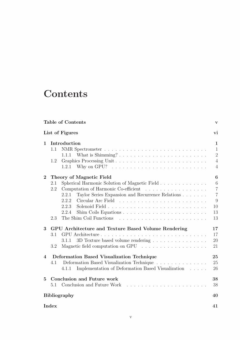
Contents
Table of Contents v
List of Figures vi
1 Introduction 11.1 NMR Spectrometer . . . . . . . . . . . . . . . . . . . . . . . . . . . . 1
1.1.1 What is Shimming? . . . . . . . . . . . . . . . . . . . . . . . . 21.2 Graphics Processing Unit . . . . . . . . . . . . . . . . . . . . . . . . . 4
1.2.1 Why on GPU? . . . . . . . . . . . . . . . . . . . . . . . . . . 4
2 Theory of Magnetic Field 62.1 Spherical Harmonic Solution of Magnetic Field . . . . . . . . . . . . . 62.2 Computation of Harmonic Co-efficient . . . . . . . . . . . . . . . . . 7
2.2.1 Taylor Series Expansion and Recurrence Relations . . . . . . . 72.2.2 Circular Arc Field . . . . . . . . . . . . . . . . . . . . . . . . 92.2.3 Solenoid Field . . . . . . . . . . . . . . . . . . . . . . . . . . . 102.2.4 Shim Coils Equations . . . . . . . . . . . . . . . . . . . . . . . 13
2.3 The Shim Coil Functions . . . . . . . . . . . . . . . . . . . . . . . . 13
3 GPU Architecture and Texture Based Volume Rendering 173.1 GPU Architecture . . . . . . . . . . . . . . . . . . . . . . . . . . . . . 17
3.1.1 3D Texture based volume rendering . . . . . . . . . . . . . . . 203.2 Magnetic field computation on GPU . . . . . . . . . . . . . . . . . . 21
4 Deformation Based Visualization Technique 254.1 Deformation Based Visualization Technique . . . . . . . . . . . . . . 25
4.1.1 Implementation of Deformation Based Visualization . . . . . 26
5 Conclusion and Future work 385.1 Conclusion and Future Work . . . . . . . . . . . . . . . . . . . . . . 38
Bibliography 40
Index 41
v
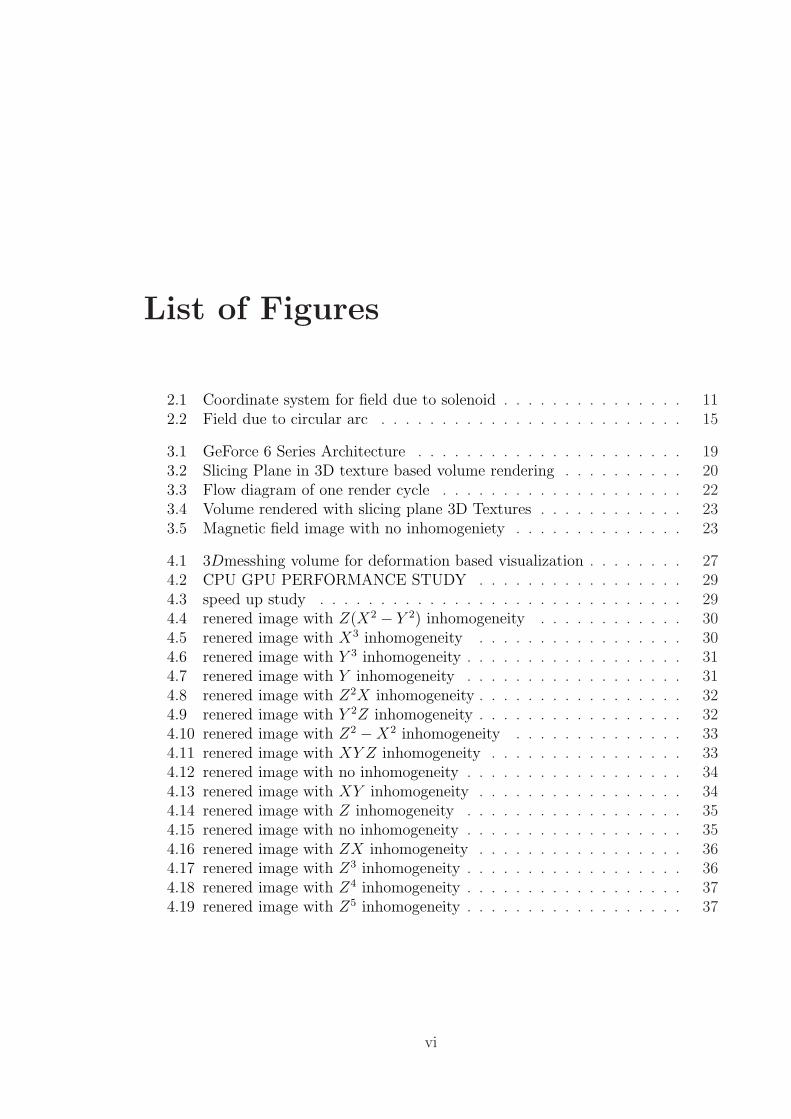
List of Figures
2.1 Coordinate system for field due to solenoid . . . . . . . . . . . . . . . 112.2 Field due to circular arc . . . . . . . . . . . . . . . . . . . . . . . . . 15
3.1 GeForce 6 Series Architecture . . . . . . . . . . . . . . . . . . . . . . 193.2 Slicing Plane in 3D texture based volume rendering . . . . . . . . . . 203.3 Flow diagram of one render cycle . . . . . . . . . . . . . . . . . . . . 223.4 Volume rendered with slicing plane 3D Textures . . . . . . . . . . . . 233.5 Magnetic field image with no inhomogeniety . . . . . . . . . . . . . . 23
4.1 3Dmesshing volume for deformation based visualization . . . . . . . . 274.2 CPU GPU PERFORMANCE STUDY . . . . . . . . . . . . . . . . . 294.3 speed up study . . . . . . . . . . . . . . . . . . . . . . . . . . . . . . 294.4 renered image with Z(X2 − Y 2) inhomogeneity . . . . . . . . . . . . 304.5 renered image with X3 inhomogeneity . . . . . . . . . . . . . . . . . 304.6 renered image with Y 3 inhomogeneity . . . . . . . . . . . . . . . . . . 314.7 renered image with Y inhomogeneity . . . . . . . . . . . . . . . . . . 314.8 renered image with Z2X inhomogeneity . . . . . . . . . . . . . . . . . 324.9 renered image with Y 2Z inhomogeneity . . . . . . . . . . . . . . . . . 324.10 renered image with Z2 − X2 inhomogeneity . . . . . . . . . . . . . . 334.11 renered image with XY Z inhomogeneity . . . . . . . . . . . . . . . . 334.12 renered image with no inhomogeneity . . . . . . . . . . . . . . . . . . 344.13 renered image with XY inhomogeneity . . . . . . . . . . . . . . . . . 344.14 renered image with Z inhomogeneity . . . . . . . . . . . . . . . . . . 354.15 renered image with no inhomogeneity . . . . . . . . . . . . . . . . . . 354.16 renered image with ZX inhomogeneity . . . . . . . . . . . . . . . . . 364.17 renered image with Z3 inhomogeneity . . . . . . . . . . . . . . . . . . 364.18 renered image with Z4 inhomogeneity . . . . . . . . . . . . . . . . . . 374.19 renered image with Z5 inhomogeneity . . . . . . . . . . . . . . . . . . 37
vi
Chapter 1
Introduction
1.1 NMR Spectrometer
Nuclear Magnetic Resonance (NMR) spectroscopy is one of the principal techniques
used to obtain physical, chemical, electronic and structural information about a
molecule. It is the only technique that can provide detailed information on the exact
three-dimensional structure of biological molecules in solution. NMR equipment re-
quires a source of magnetic field with minimal inhomogeneities. No magnet generates
an ideal homogeneous magnetic field and therefore a complicated system of coils is
required. Coils fed by separate current supplies to remove particular magnetic inho-
mogeneity (X, Y, Z, XY, Y Z, XZ, X2 − Y 2, XZ2, Y Z2, Z, Z2, Z3, Z4) is needed. For
a solenoid magnet with a cylinder shaped work space, the individual active shims
consists of circular and saddle shaped coils symmetrically positioned on the co-axial
cylindrical surfaces.
The theory of magnetic field due to a known coil geometry is well established.
Significant research has gone into computational aspect of the magnetic field. The
theory, design and construction of a magnetically shielded solenoid is described in [1],
1
1.1 NMR Spectrometer 2
[2], [3]. High resolution magnet for NMR and MRI based on the spherical harmonics
and unique recursion relations for the co-efficient of most dominant components is
described in [4].
1.1.1 What is Shimming?
In the beginning, the field homogeneity of large electromagnets was adjusted by me-
chanical alignment of the magnet pole faces. The more parallel the pole faces, the
more homogeneous the magnetic field. The first step in the process of adjusting mag-
netic homogeneity was to adjust the position of the magnet’s pole faces by turning
three large bolts which held the pole faces. Adjusting these bolts tilted the pole faces
relative to each other with the aim of making the pole faces more parallel. If the
bolts ran out of range, thin pieces of brass were placed between the magnet yoke
and the pole pieces to move the pole pieces as parallel as possible. These thin pieces
of brass were also placed in other strategic locations to make the pole faces parallel
in a manner not addressed by the three adjustment bolts. The metal pieces were
called shim stock and the seemingly endless process of placing and removing pieces
of shim stock acquired the name ”shimming”. Because tons of magnetic field pres-
sure existed on the pole faces, the magnet had to be turned off to place and remove
the shim stock. When the sample was spinning, the final part of adjusting magnetic
homogeneity with these systems was to adjust a ratchet bolt which pulled together
or pushed apart the tops of the magnet pole pieces to give a fine adjustment of the Y
gradient. All of these processes were mechanical in nature. After these adjustments,
the NMR instruments were typically capable of giving better than 0.2 Hz resolution.
This is rather impressive when you consider that 0.2 Hz out of 60 MHz represents 3
parts per billion field homogeneity over the volume of the sample.
To increase the performance, reduce the difficulty of adjusting magnetic homo-

1.1 NMR Spectrometer 3
geneity and reduce the manufacturing difficulty of the magnets, an electronic ”shim-
ming” process was developed which used a series of small electromagnets having very
specific magnet field contours. These small electromagnets are placed around the
sample area. Each small electromagnet can be used to adjust the field in the volume
of observation to create more of or counteract existing types of magnetic gradients.
A complete series of these electromagnets can be used to adjust the magnetic field
homogeneity to a given level of purity depending on how many types of adjustment
electromagnets are used. The process of adjusting the magnetic field homogeneity by
adjusting the current in each of the small electromagnets retained the name shimming
and the small electromagnets assumed the name ”shims”.
At first only a few low order ( X, Y , and Z) electrical shims were used. As the
fields became higher, magnet production became more difficult, and more and higher
order electrical shims were added to maintain the same level of performance. These
electrical shims are not 100% pure and have interactions with shims of a similar
nature ( ZX creates some Z gradient and X gradient in addition to the intended ZX
gradient ). Because of these interactions, the number of adjustments necessary to
shim the magnet increases geometrically with the number of shims, not just linearly.
In addition, the raw field encountered in superconducting magnets is usually worse
than in electromagnets, so larger corrections are required. These two facts make
the process of shimming superconducting magnets more difficult and the shimming
process more important to obtain useful NMR spectra.
To obtain 0.2 Hz resolution requires ten times greater magnetic field homogeneity
at 600 MHz than at 60 MHz. Therefore, in addition to the higher field supercon-
ducting magnets being more difficult to shim, shimming becomes more important to
obtain the same results as the magnetic fields increase. Other aspects of an NMR
instrument’s performance are also affected by shimming, such as the NMR signal’s
1.2 Graphics Processing Unit 4
lineshape, which is critical for achieving good solvent suppression. So the necessary
evil of adjusting the small electromagnets, called shimming, remains very important
in today’s NMR instrumentation.
1.2 Graphics Processing Unit
GPUs have evolved as a fully programmable and immensely parallel workhorse for
graphics computation. Availability of high-level languages and tools have led to ex-
plosion of innovation and creativity. Programmability allows for running any task
on GPU as long as an algorithm can be found that fits into the streaming model.
GPGPU (General Purpose Computation on GPU) applications [5] ranges from nu-
meric computing operation such as dense and sparse matrix multiplication technique
or multi-grid conjugate gradient solvers for system of linear equations to computer
graphics processes such as ray tracing and photon mapping usually performed offline
in CPU, to physical simulations such as fluid mechanics solvers ,to data base and
data mining operations. The physics based simulation on GPU was first seen in [5],
which also demonstrated the ”Game of Life” cellular automata and a 2D physically
based wave simulation. Several researcher has used GPU to simulate fluid dynamics.
Related to fluid simulation is visualizations of flow which has been implemented us-
ing graphics hardware to accelerate line integral convolution an Lagrangian-Eulerian
advection.
1.2.1 Why on GPU?
Shimming the NMR magnet is a complex task.The most common method of adjusting
the homogeneity of an NMR magnet is the observation of an NMR signal. The
problem with the shimming process is that the observed NMR signal results from
1.2 Graphics Processing Unit 5
the integrated signal from the total volume of the observed sample, which may have
many different resonant frequencies with different degrees of excitation arising from
different positions in the sample. NMR sample can be visualized as a continuum of
isolated mini-samples, each of which is infinitesimally small. Each mini-sample then
generates a signal whose linewidth is determined by the T2 relaxation time of the
sample and whose frequency results from the field value at that point. The intensity
of the signal generated by each mini-sample would reflect the amount of excitation
at that point. What the NMR operator observes is the sum of signals from all the
mini-samples. In other words, the NMR signal is the total integrated signal over the
total sample volume times each area’s degree of excitation. It is the integration of
the NMR signal response which leads to a major difficulty in the shimming process.
Any knowledge as to which part of the NMR sample is experiencing the magnetic
inhomogeneity is lost in this integration process. Thus, to overcome above difficulty,
instead of signals the magnetic field inside sample volume needed to be visualized.
Though, scalar field visualization is solved problem but visualizing magnetic field in
the context of shimming poses two challenges:
1: It should be interactive. For an interactive application at least 20-30 frame per
second is needed.
2: The type of inhomogeneity present should be identified from the rendered
image.
Because of inherent parallelism GPUs are highly efficient for data and compute
intensive operations. To achieve required frame rate it is implemented on GPU.

Chapter 2
Theory of Magnetic Field
2.1 Spherical Harmonic Solution of Magnetic Field
The total magnetic induction in a homogeneous region containing no field sources
is described by the Laplace equation. NMR applications employ magnets that are
axially symmetric [2].
∇2Bz = 0 (2.1)
The dominant component Bz, parallel to the symmetry axis is also described by
the Laplace equation in the form Eq.(2.1) The solution of Eq.(2.1) can be expressed
in spherical harmonic expansion
Bz(x, y, z) =∞∑
n=0,m=0
rnmPn(cos θ) × [am,n cos (mϕ) + bm,n sin (mϕ)] (2.2)
where r, θ and φ are spherical coordinates, am,n and bm,n are coefficients and
mPn(cos θ) are associated Legendre polynomials of first kind, degree n and order m.
The first member of Eq.(2.2) is the ideal homogeneous field. Eq.(2.2) can be expanded
in Cartesian coordinates as in Eq.(2.3), shown only up to third degree and order.
6
2.2 Computation of Harmonic Co-efficient 7
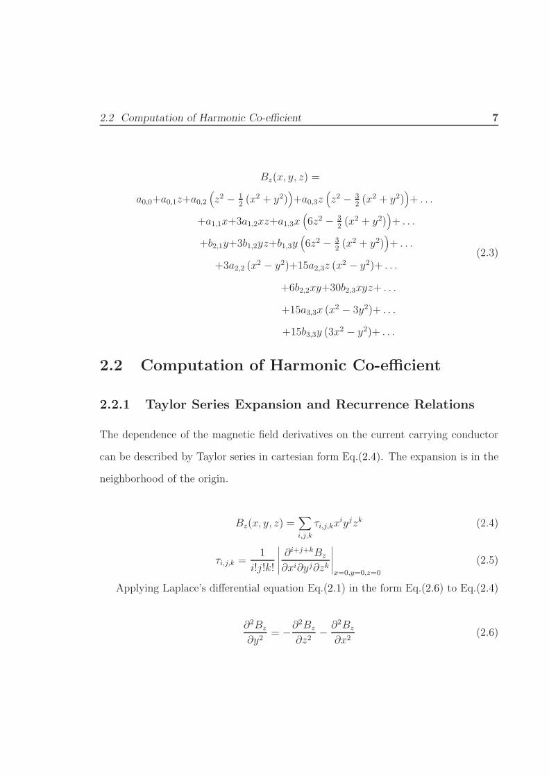
Bz(x, y, z) =
a0,0+a0,1z+a0,2
(
z2 − 12(x2 + y2)
)
+a0,3z(
z2 − 32(x2 + y2)
)
+ . . .
+a1,1x+3a1,2xz+a1,3x(
6z2 − 32(x2 + y2)
)
+ . . .
+b2,1y+3b1,2yz+b1,3y(
6z2 − 32(x2 + y2)
)
+ . . .
+3a2,2 (x2 − y2)+15a2,3z (x2 − y2)+ . . .
+6b2,2xy+30b2,3xyz+ . . .
+15a3,3x (x2 − 3y2)+ . . .
+15b3,3y (3x2 − y2)+ . . .
(2.3)
2.2 Computation of Harmonic Co-efficient
2.2.1 Taylor Series Expansion and Recurrence Relations
The dependence of the magnetic field derivatives on the current carrying conductor
can be described by Taylor series in cartesian form Eq.(2.4). The expansion is in the
neighborhood of the origin.
Bz(x, y, z) =∑
i,j,k
τi,j,kxiyjzk (2.4)
τi,j,k =1
i!j!k!
∣
∣
∣
∣
∣
∂i+j+kBz
∂xi∂yj∂zk
∣
∣
∣
∣
∣
x=0,y=0,z=0
(2.5)
Applying Laplace’s differential equation Eq.(2.1) in the form Eq.(2.6) to Eq.(2.4)
∂2Bz
∂y2= −
∂2Bz
∂z2−
∂2Bz
∂x2(2.6)

2.2 Computation of Harmonic Co-efficient 8
we have
Bz(x, y, z) =
τ0,0,0+τ0,0,1z+τ0,0,2
(
z2 − y2)
+τ0,0,3z(
z2 − 3y2)
+ . . .
+τ1,0,0x+2τ1,0,1xz +2τ1,0,2x(
z2 − y2)
+ . . .
+τ0,1,0y+2τ0,1,1yz +τ0,1,2y(
3z2 − y2)
+ . . .
+τ2,0,0
(
x2 − y2)
+3τ2,0,1z(
x2 − y2)
+ . . .
+2τ1,1,1xy +6τ1,1,1xyz+ . . .
+τ3,0,0x(
x2 − 3y2)
+ . . .
+τ2,1,0y(
3x2 − y2)
+ . . . (2.7)
The polynomial in the M th row and nth column of the expansion Eq.(2.7) can be
denoted by MTn, the following recursion formulae can be adopted.
0Tn = z0Tn−1 − y2Tn−1
n = 1, 2, 3, ... (2.8)
1Tn = nx0Tn−1
2Tn = y0Tn−1 + z2Tn−1
MTn = 2n(
xM−2Tn−1 − yM−1Tn−1
)/
(M + 1)
(2.9)
for odd M = 3, 5, ..., 2n − 1 and
MTn = zMTn−1 + xM−2Tn−1 + yM−3Tn−1 (2.10)
for even M = 4, 6, ..., 2n. where 0T0 = 1 and 2nTn−1 = 0.
Eq.(2.3) and Eq.(2.7) describes the same field. Their members with identical
powers of the individual coordinates can be compared and the relationship between

2.2 Computation of Harmonic Co-efficient 9
the coefficients can be determined. The coefficients am,n and bm,n are specified as the
linear combination of the derivatives τi,j,k, i + j + k = n.
2.2.2 Circular Arc Field
Bz due to a current carrying circular arc of conductor as shown in Fig.2.2. at a point
(x, y, z) is given by Biot-Savart law, Eq.(2.11).
Bz(x, y, z) =µIr
4π×
φ∫
−φ
(r − x cos ξ − y sin ξ) dξ[
x2 + y2 + (z − d)2 − 2r (x cos ξ + y sin ξ) + r2]3/2
(2.11)
where I is the current in the circular conductor of radius r and arc angle 2φ, d
is the z coordinate of the plane containing the circular arc. µ is the permeability
of the medium and the ξ is the integration variable. By evaluating the derivatives
of Eq.(2.11) as specified by Eq.(2.5) at the origin, the τi,j,k are obtained and are
consecutively transformed to spherical harmonic coefficients am,n and bm,n. For the
given pose of circular arc bm,n = 0. By further analysis am,n can be found out by
exploiting the recurrence relation and rotary symmetry. Coefficients for the zonal
members (rotary symmetry,m=0) are given by formula
a0,n = Cn0Znφ (2.12)
Where Cn equals µI/2πccnn!. Using β = d/c for the relative position of the
current carrying arc 0Zn is determined by the recursion formula
pZq = −(2q + 1)pZq−1 + [q2 − (p − 1)2]pZq−2
1 + β2(2.13)
where p = 0 and q = 1, 2, 3....n successively, the starting functions being

2.2 Computation of Harmonic Co-efficient 10
0Z0 = (1 + β2)−3/2
and 0Z0 = 0
The Coefficients for the tesseral (n > m > 0) and sectorial terms (independent of
z coordinate , n = m) are calculated using expression
am,n = Cn
[
m∏
i=1
|(2i − 3)|
n + i
]
×[(
4m2 − 1)
mZn − m−2Zn
] sin mφ
m(2.14)
where mZn and m−2Zn are auxiliary functions for the degree n = 1, 2, 3, ... and the
order m = 1, 2, 3..... They are given by formula (2.13) with generalized starting
functions
pZp=q = (1 + β2)−p−(3/2)
and pZq<p = 0.
An application of these relations to calculate the starting functions is demon-
strated for m=1; the determination of the function 1Zn begins with 1Z0 = 0 and
1Z1 = (1 + β2)−2.5
, similarly, that of −1Z−2 = 0 and 1Z1 = (1 + β2)−0.5
.
2.2.3 Solenoid Field
To describe the spatial variation of the field it is most convenient to use an expansion
in spherical harmonics. The field is completely specified if the field on the axis of the
symmetry is known [1].
The coordinate system used to describe the field are shown in Fig.2.1. A given
point in the solenoid can be described by its spherical coordinates(r, θ, φ) or its cylin-
drical coordinates (ρ, φ, z). To describe the magnetic field we shall use the components
parallel to and perpendicular to the axis of symmetry as in Eq.(2.15).
H = k · Hz(r, θ) + γHρ(r, θ) (2.15)
where γ and k are unit vectors in the ρ and z directions, respectively. Since the

2.2 Computation of Harmonic Co-efficient 11
L/2 L/2
asr s
θs
oz
ρ
θ
r
(r,θ,φ)
(ρ,φ,z)
symmetry
axis
(a)
(b)
Figure 2.1 (a): Coordinate system used to describe the field in axially
symmetric system.(b): coordinate used to specify the single layer of the solenoid of length Land radius as.

2.2 Computation of Harmonic Co-efficient 12
system of conductors is axially symmetric, the magnetic field will not be a function of
the azimuthal angle φ. We write the potential inside the system of conductors with
cylindrical geometry as Eq.(2.16).
V (r, θ) =∞∑
n=1
(
−Hn−1
n
)
rnPn(cos θ) (2.16)
where Pn(cosθ) is a Legendre polynomial. The potential function gives the radial
and axial components as in Eq.(2.17) and Eq.(2.18).
Hz(r, θ) =∞∑
n=1
HnrnPn(cos θ) (2.17)
Hρ(r, θ) =∞∑
n=1
(
1
n + 1
)
Hnrn d
dθPn(cos θ) (2.18)
Where the coefficient Hn are given by the relationship in Eq.(2.19) and Eq.(2.20).
Hn =(
1
n!
)
[(
dn
dzn
)
Hz(z, 0)
]
z=0
(2.19)
Hz(z, 0) =4π
10
NsI
2rs×
1 −
[
1 − (us)2
us
]
×∞∑
n=1
(
1
2n
)(
z
rs
)2n
P ′
2n(us)
(2.20)
Here Ns is the total number of turns, us is for cosθs, I is the current, and P ′
2n(us) =
(d/dus) P2n(us)
The magnetic field is in gauss if I is in amperes and rs is in centimeters. Due to
the plane of symmetry through the origin odd powers of z in the expression Eq.(2.20)
is zero. We can rewrite Eq.(2.20) in series form as Eq.(2.21).

2.3 The Shim Coil Functions 13
Hz(z, 0) =4πNI
10(cos θs) ×
1 −3
2sin4 θs
(
z
as
)2
−5
8
(
sin6 θs
) (
7 cos2 θs − 3)
(
z
as
)4
−7
16
(
sin8 θs
)
×(
33 cos4 θs − 30 cos2 θs + 5)
(
z
as
)6
− . . .
(2.21)
Here N is the number of turns per unit length. The successive terms of this
expression will be referred to as the zero-order term, second-order term, the fourth-
order term, etc.
2.2.4 Shim Coils Equations
Shim coils are designed to produce gradient fields to compensate for the inhomo-
geneities in the field due to the main solenoid. The currents in the coil are inde-
pendently controlled to give maximum freedom for tuning. In order to make the
field as homogeneous as possible, the derivatives of the axial field Bz at the origin
should be minimized or made zero by using the shim coils. This is one of the design
consideration for the shim coils. Detailed geometric design of X-shim coils is given
in table2.1. For the purpose of further computation and visualization we consider
typical geometric design for main solenoid and shim coils and derive the coefficients.
The spherical harmonic coefficients am,n and bm,n of typical shim coils are listed in
Table-2.2.
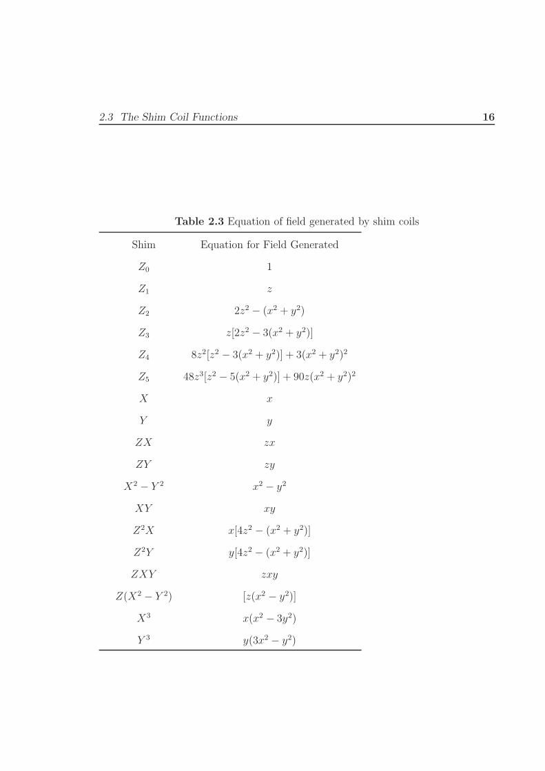
2.3 The Shim Coil Functions
In previous sections the theory to compute coefficients of spherical harmonics for dif-
ferent geometry is described. In table 2.2 co-efficients for X shim is described.Ideally

2.3 The Shim Coil Functions 14
Table 2.1 The parameters for X shim coil design
Nominal radius r 25mm
Conductor cross section 0.7mm × 0.035mm
Nominal current 100.0mA
Length of winding 12.4m
Resistance at 200C 8.8Ω
Table 2.2 Values of the spherical harmonic coefficients for the coils derived
from the coil geometry. The coefficients are in µtesla.
Main solenoid
a0,0 = 7.5 × 10⁶ a0,1 = 4.2 × 10² a0,2 = 4.1 × 10² a0,3 = 3.1 × 10⁻¹
a1,1 = 5.2 × 10² a1,2 = 3.2 × 10² a1,3 = 5.1 × 10⁻¹
b1,1 = 5.2 × 10² b1,2 = 1.2 × 10² b1,3 = 5.1 × 10⁻¹
a2,2 = 4.4 × 101 a2,3 = 2.1 × 101
b2,2 = 1.2 × 101 b2,3 = 5.2 × 101
a3,3 = 9.2 × 101
b3,3 = 9.2 × 101
X Shim coil
a0,0 = 0.1 × 10⁻⁴ a0,1 = 2.1 × 10⁻² a0,2 = 4.1 × 10⁻² a0,3 = 3.1 × 10⁻²
a1,1 = 3.4 × 10² a1,2 = −4.4 × 10⁻² a1,3 = 5.1 × 10⁻¹
b1,1 = −5.2 × 10⁻² b1,2 = −1.2 × 10⁻² b1,3 = 5.1 × 10⁻¹
a2,2 = 2.4 × 10⁻² a2,3 = 2.1 × 10⁻³
b2,2 = 6.2 × 10⁻² b2,3 = 5.2 × 10⁻²
a3,3 = 9.2 × 10⁻³
b3,3 = 1.2 × 10⁻³

2.3 The Shim Coil Functions 15
z
y
x
θ
r
ϕ
-dc
I
φ−φ
Βz
Figure 2.2 Coordinates for the computation of the field Bz(x, y, z) of a
current filament in the form of circular arc.
, X-shim coil should have only a1,1 coeffiecients other coefficients should be zero.But
it is impossible to design totally pure X-shim coil. The various shim coils and there
functions are described in table 2.3.The design parameter for this coil is not avail-
able in literature, these are mostly patented. So for our simmulation purpose we
considered that the shim coils field are completely pure.
2.3 The Shim Coil Functions 16
Table 2.3 Equation of field generated by shim coils
Shim Equation for Field Generated
Z0 1
Z1 z
Z2 2z2 − (x2 + y2)
Z3 z[2z2 − 3(x2 + y2)]
Z4 8z2[z2 − 3(x2 + y2)] + 3(x2 + y2)2
Z5 48z3[z2 − 5(x2 + y2)] + 90z(x2 + y2)2
X x
Y y
ZX zx
ZY zy
X2 − Y 2 x2 − y2
XY xy
Z2X x[4z2 − (x2 + y2)]
Z2Y y[4z2 − (x2 + y2)]
ZXY zxy
Z(X2 − Y 2) [z(x2 − y2)]
X3 x(x2 − 3y2)
Y 3 y(3x2 − y2)

Chapter 3
GPU Architecture and Texture
Based Volume Rendering
3.1 GPU Architecture
General purpose computation on GPUs [6] is being advocated in various non graph-
ics areas. Applications have been found in numerical computation, cryptography ,
signal processing, and many others [5]. GPUs were designed as efficient coproces-
sors for rendering and shading. The programmability now available in GPUs such as
the NVIDIA GeForce series makes them useful coprocessors for more diverse applica-
tions. Several programming languages are made available for creatively exploiting the
GPU for non-graphic applications. OpenGL Shading Language (GLSL) [7], nVidia’s
C for Graphics (Cg) [8], and Microsoft’s High Level Language (HLSL) [9] are some
examples. Since the time between new generations of GPUs is currently much less
than for CPUs, faster coprocessors are available more often than faster central pro-
cessors. GPU performance tracks rapid improvements in semiconductor technology
more closely than CPU performance. This is because CPUs are designed for high
17

3.1 GPU Architecture 18
performance on sequential operations, while GPUs are optimized for the high par-
allelism of vertex and fragment processing . Additional transistors can therefore be
used to greater effect in GPU architectures. In addition, programmable GPUs are
inexpensive, readily available, easily upgradeable, and compatible with multiple op-
erating systems and hardware architectures. More importantly, interactive computer
graphics applications have many components vying for processing time. Often it is
difficult to efficiently perform simulation, rendering, and other computational tasks
simultaneously without a drop in performance. Since our intent is visual simulation,
rendering is an essential part of any solution. By moving simulation onto the GPU
that renders the results of a simulation, it not only reduce computational load on
the main CPU, but also avoid the substantial bus traffic required to transmit the re-
sults of a CPU simulation to the GPU for rendering. In this way, methods of dynamic
simulation on the GPU provide an additional tool for load balancing in complex inter-
active applications. For the purpose of clarity here a brief model of GPU is presented
(Fig.3.1) . Detailed information can be found at [10]. It contains a vertex engine,
fragment engine, a texture load/filter engine, and a depth-compare/blend data write
engine. The vertex and the fragment processors are the user programmable stages
of the pipeline. Vertex and fragment blocks operate on data serially and they both
support floating point operands. The vertex processor operates on data, passing it
directly to the fragment processor, or by using the rasterizer to expand the data into
the interpolated values. Each triangle (or point) fed to the vertex processor becomes
one or more fragments. The GPU support 16 bit floating point for four color com-
ponents allowing for high dynamic range. GPUs differ by the shader capabilities and
are identified by a particular shader model. nVidia GeForce 6 supports Shader Model
3.0.
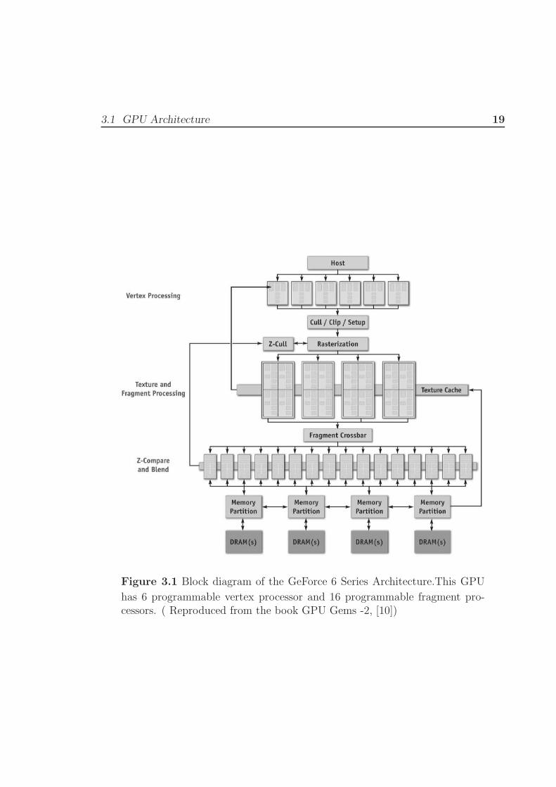
3.1 GPU Architecture 19
Figure 3.1 Block diagram of the GeForce 6 Series Architecture.This GPU
has 6 programmable vertex processor and 16 programmable fragment pro-cessors. ( Reproduced from the book GPU Gems -2, [10])

3.1 GPU Architecture 20
Figure 3.2 3D texture and slicing planes orthogonal to the view direction.
Higher number of planes sample the scalar field more closely but increasesthe GPU passes.
3.1.1 3D Texture based volume rendering
CPU based scalar field visualization is highly compute intensive and is slow for real
time interaction. One particular technique of interest is the one that uses hardware
accelerated texture mapping [11]. This technique essentially resamples the scalar field
(volume data set) that is represented as a series of 2D textures. A ghost plane normal
to the viewing direction slices the scalar field and samples the sectional view, shown
in Fig.3.2. GPU supports the necessary sampling techniques including the trilinear
interpolation. An advanced technique was proposed by [12] that demonstrates both
interactive volume reconstruction and interactive volume rendering with hardware
provided 3D texture acceleration. The number of slicing planes or ghost planes is
decided by the resolution of the 3D texture and the desired quality of rendering.
The order of rendering of the slicing plane decides the alpha blending function. For
3.2 Magnetic field computation on GPU 21
front-to-back order requires Eq.(3.1), where as back-to-front requires Eq.(3.2). Where
Cdest, αdest are destination color and alpha, Csrc, αsrc are source color and alpha re-
spectively.
Cdest = (1 − αdest) αsrcCsrc + Cdest
αdest = αdest + (1 − αdest)αsrc
(3.1)
Cdest = (1 − αsrc) Cdest + αsrcCsrc (3.2)
Rendering each plane requires one pass of GPU process. Some GPUs support
multiple render targets (MRTs) wherein 4 or more pass can be included in a single
rendering cycle. This feature particularly helps to speed up intermediate computation.
3.2 Magnetic field computation on GPU
This section concentrates on the generation of magnetic field on GPU as a function
of main coil and shim coil currents. Our first approach involves precomputing the
3D textures for various shim coil geometries and then linearly combining them in
the GPU. The total magnetic field is described by BTotalz = I0B
Mainz + I1B
Shim1
z +
I2BShim2
z + · · · is the magnetic field due to a unit current and Ii, i = (0, 1, 2...) is the
current factor. User interface provides the slider bars to change the Ii, which is then
encoded into an ’Uniform Parameter’ array for the fragment shader program. The
basic flow diagram is explained in Fig.3.3. We precompute the magnetic field 3D
textures using Eq.(2.7) or Eq.(2.3) and coefficients from Table-2.2. the quad planes
are supplied with proper 3D texture coordinates. A vertex shader program is written
that transforms the quad plane and its texture coordinates to make it orthogonal to
the view direction. The output of the vertex shader is fed to the fragment shader
whose pseudo code is presented in Table-3.1.
tex3D(., .) is the function to access the 3D texture given the texture coordinates

3.2 Magnetic field computation on GPU 22
Figure 3.3 Flow diagram of one render cycle. Ii is encoded into an array
and set as uniform parameter to the fragment shader.
texcoord.xyz. GPU generates the texture coordinates by interpolation, in our case
it is set to trilinear. GPU allows for simultaneous operations on various data paths.
The algorithm that is presented in Table-3.1 is parallelized in the GPU and hence
several order of speedup is possible.
Precomputing 3D textures is compute-intensive task and it is best done in the
GPU itself. Higher number of shim coils demand that many number of 3D Textures,
which directly increases the memory requirement in O(m∗n3), where m is the number
of 3D textures and n is the size of the texture. For n = 256 and m = 16 the memory
requirement would be roughly 1024 MB, with 32 floats for each voxel. Latest graphics
card doesnot have support for 1024 MB of memory. Thus, texture data will be
stored in disk.Thus transfering data from disk to GPU will hurt the performance
of the programme. To this end we propose an alternative algorithm that requires
less memory but takes up more GPU computation. For each slice plane we compute
the magnetic field directly from Eq.(2.3) or Eq.(2.7). This method as described in
Table-3.2 still delivers the required frame rate for interactive rendering.
3.2 Magnetic field computation on GPU 23
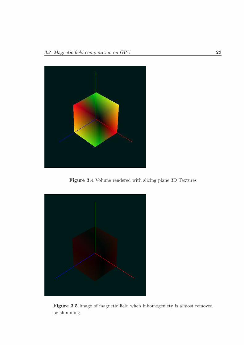
Figure 3.4 Volume rendered with slicing plane 3D Textures
Figure 3.5 Image of magnetic field when inhomogeniety is almost removed
by shimming

3.2 Magnetic field computation on GPU 24
Table 3.1 Fragment shader for summing up the fields due to various shim
coils.
float Bz0 = tex3D(Bz1Texture, texcoord.xyz);
float Bz1 = tex3D(Bz2Texture, texcoord.xyz);
// Sum up weighted components
BzTotal = I0 * Bz0 + I1 * Bz1 + ...
// Adjust to fit in 0.0 to 1.0
ScaleShift(BzTotal);
float4 color.rgba = tex1D(colormap, BzTotal);
Table 3.2 Algorithm for direct field computation. We embed Eq.(2.3) in the
fragment shader.The coefficients am,n are set as uniform parameters to thefragment program.
// Evaluate Eq.(2.3)(or Eq.(2.7))
float BzTotal = Evaluate( texcoord.xyz ) ;
// Adjust to fit in 0.0 to 1.0
ScaleShift(BzTotal);
float4 color.rgba = tex1D(colormap, BzTotal);
Chapter 4
Deformation Based Visualization
Technique
4.1 Deformation Based Visualization Technique
Texture based volume rendering produces an image by mapping color to different
type of inhomogeneity. Many different kind of inhomogeneity combine together to
produce a single color.Thus,what kind of inhomogeneity has produced the color can-
not be made out from the image .3.4 Subsequently, which shim coil to be adjusted
to remove homogeneity cannot be decided from the image. Thus, to overcome that
difficulty we propose an alternate visualization technique which deforms the geometry
of visualization volume. The deformation geometry depends on the type of inhomo-
geneity present in the field. The cube shaped visualization volume is divided into
a uniform 3D grid. All point on the grid occupied the original position if there is
no inhomogeneity present in the field. The points get displaced from their original
position if there is any inhomogeneity present in it. The displaced position of the
25

4.1 Deformation Based Visualization Technique 26
points are given by equation (4.1).
P ′ = P + c∇Bz (4.1)
Where P ′ is the position of the point P when a nonuniform magnetic field Bz is
applied in the volume.c is a constant to be chosen carefully to accentuate inhomogene-
ity. If small value of c is chosen then effect of inhomogeneity cannot be visible where
as larger value of it will increase the size of image . As homogeneity is approached by
optimally adjusting shim currents the deformation decreases. Thus to make deforma-
tions noticable the parameter c is increased gradually. If the field is homogeneous then
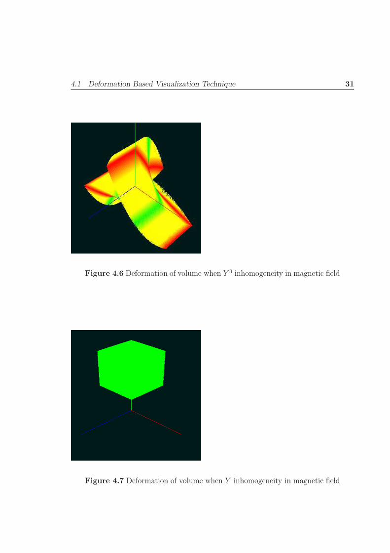
∇Bz vanishes and volume remains undeformed. If a linear inhomogeneity is present
then each point in the volume will be displaced by a constant distance which resulted
in translation of volume without any deformation. From the direction of tanslation it
is possible to shim either of X, Y, Z coil to correct it. Other types of inhomogeneities
will produce various deformed volume. The deformation of volume due to various
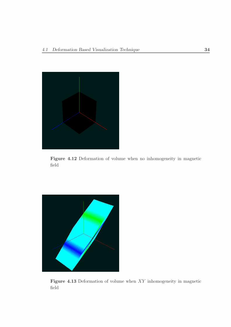
inhomogeneity are shown in figure(4.4 through 4.19 ). The shim current which needs
adjustment can be identified easily just looking at the deformed volume.
4.1.1 Implementation of Deformation Based Visualization
To implement it a vertex shader programme is developed to render deformed volume
as given in algorithm (3.2). The visualization system being used is Pentium-4 work
station with n-Vidia GeForce 6600 graphics card, running Linux SUSE10. All graphics
programmes are written using OpenGL. The volume is meshed to a m×m×m grid
,m being the number of point in each dimension.The grid for is shown in figure(
m = 84.1).At each grid point the magnetic field and gradient is computed using
equation 2.3 .From magnetic field gradient the position of each grid point is computed.
They are implemented in CPU. Then the data is transfered to GPU for visualization.

4.1 Deformation Based Visualization Technique 27
Figure 4.1 3Dmesshing volume for deformation based visualization. The
volume is divided into 8× 8× 8 gridpints.The grid point changes there posi-tions depending on the inhomogeneity present in the field.
However with this implementation when grid size exceeds 64×64×64 , the rendering
becomes slower for user interactions. To over come that difficulty , the magnetic
field value and gradient are computed on GPU itself. A vertex shader is written
in assembly to optimize the performance. The color and alpha value are computed
to emphasize the point having high inhomogeneity .This is done by assigning alpha
value to the modulous of gradient. The red, green and blue colors are assigned to the
absolute value of each component of the field gradient.

4.1 Deformation Based Visualization Technique 28
Table 4.1 Algorithm for deformable volume based visualization . A vertex
shader programme is developed to compute the position of points inside thedeformable volume
// Evaluate Eq.(2.3)(or Eq.(2.7))
float BzTotal = Evaluate( vertexpos.xyz ) ;
// Compute gradient and save it in 3D vector
vector3d grad.xyz =gradient(BzTotal)
// Compute position
Position.xyz =Position.xyz+c*grad.xyz
// Compute alpha value and color
// alpha value is the magnitude gradient
alpha=MagGradient(grad.xyz)
// color value is absolute value of each component gradient
color.rgb=ABS(c*grad.xyz)
4.1 Deformation Based Visualization Technique 29
0 50 100 150 200 250 3000
1
2
3
4
5
6
Grid Size
Tim
e in
sec
ond
CPU timeGPU time
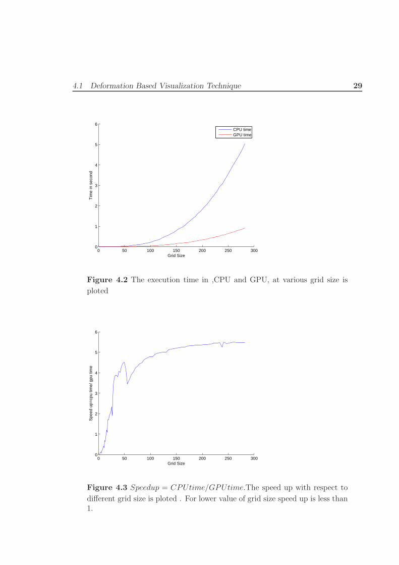
Figure 4.2 The execution time in ,CPU and GPU, at various grid size is
ploted
0 50 100 150 200 250 3000
1
2
3
4
5
6
Grid Size
Spe
ed u
p=cp
u tim
e/ g
pu ti
me
Figure 4.3 Speedup = CPUtime/GPUtime.The speed up with respect to
different grid size is ploted . For lower value of grid size speed up is less than1.

4.1 Deformation Based Visualization Technique 30
Figure 4.4 Deformation of volume when Z(X2−Y 2) inhomogeneity in mag-
netic field
Figure 4.5 Deformation of volume when X3 inhomogeneity in magnetic field
4.1 Deformation Based Visualization Technique 31
Figure 4.6 Deformation of volume when Y 3 inhomogeneity in magnetic field
Figure 4.7 Deformation of volume when Y inhomogeneity in magnetic field

4.1 Deformation Based Visualization Technique 32
Figure 4.8 Deformation of volume when Z2X inhomogeneity in magnetic
field
Figure 4.9 Deformation of volume when Y 2Z inhomogeneity in magnetic
field

4.1 Deformation Based Visualization Technique 33
Figure 4.10 Deformation of volume when Z2 − X2 inhomogeneity in mag-
netic field
Figure 4.11 Deformation of volume when XY Z inhomogeneity in magnetic
field
4.1 Deformation Based Visualization Technique 34
Figure 4.12 Deformation of volume when no inhomogeneity in magnetic
field
Figure 4.13 Deformation of volume when XY inhomogeneity in magnetic
field

4.1 Deformation Based Visualization Technique 35
Figure 4.14 Deformation of volume when Z inhomogeneity in magnetic field
Figure 4.15 Deformation of volume when no inhomogeneity in magnetic
field
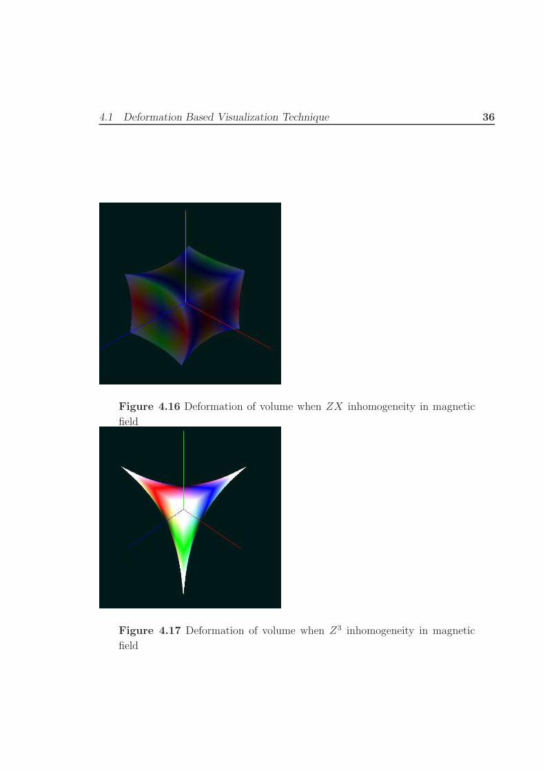
4.1 Deformation Based Visualization Technique 36
Figure 4.16 Deformation of volume when ZX inhomogeneity in magnetic
field
Figure 4.17 Deformation of volume when Z3 inhomogeneity in magnetic
field

4.1 Deformation Based Visualization Technique 37
Figure 4.18 Deformation of volume when Z4 inhomogeneity in magnetic
field
Figure 4.19 Deformation of volume when Z5 inhomogeneity in magnetic
field

Chapter 5
Conclusion and Future work
5.1 Conclusion and Future Work
The result of our texture based volume rendering is shown in figure [3.4][3.5]. When
field is completely homogeneous the rendered image should look like image [3.5].
Though, deformable grid based visualiaztion technique involves an over head of com-
puting gradient of the field at each grid points, but image produced by this technique
can be used to identify the inhomogeniety present in the field. With the vertex pro-
gramme gradient of magnetic field is computed on GPU itself which provides enough
frame rates for user interaction.A comparative study is given in figure [4.3,4.2].For
the lower grid size the speed up is less than 1.However for better quality image we
need to have greater grid size.For more than 25 × 25 × 25 grid size the speed up is
more than one. The result of deformation based visualization is shown in figure [4.4
through 4.19 ]
While computing the magnetic field the magnetic properties of the sample is not
taken into consideration.The magnetic field distortion due to magnetic properties of
sample is considerable at the edge of the sample.There are numerical models available
38

5.1 Conclusion and Future Work 39
to compute magnetic field distortion due to sample. Thus, in future this effect can
be modelled and implemented.

Bibliography
[1] R. J. Hanson and F. M. Pipkin, “Magnetically Shielded solenoid with field of
High homogeneity,” The Review of scientific Instruments 36 (1965).
[2] J. Dadok, “Shim coils for superconducting solenoids,” Abstracts of the 10th
Experimental NMR conference (1969).
[3] I. Dolezal and K. Sveda, “Shim coil for NMR solenoid,” Elektrotechnicky casopis
26 (1975).
[4] M. D. Sauzade and S. K. Kan, “High resolution nuclear magnetic resonace spec-
troscopy in magnetic fields,” Electron. Electron Phys. 34 (1973).
[5] J. D. Owen, D. Luebke, N. Govindraju, M. Harris, J. Kugger, A. E. Lefohn, and
T. J. Purcell, “A Survey of General Purpose computation on Graphics hardware,”
EUROGRAPHICS (2005).
[6] GPGPU:, “General Purpose Computation on GPU,” http://www.gpgpu.org
(2006).
[7] “OpenGL Shader Language,” http://www.lighthouse3d.com/opengl/glsl/ .
[8] R. Fernando and M. J. Kilgard, CG Tutorial: A Definitive Guide (Addision and
Wesley, 2003).
40

BIBLIOGRAPHY 41
[9] “HLSL,” http://www.neatware.com/lbstudio/web/hlsl.html .
[10] M. Pharr, GPUGems2 :Programming Techniques for High-Performance Graphics
and General-Purpose Computation (Addison-Wesley, 2005).
[11] T. J. Cullip and U. Neumann, “Accelerating volume reconstruction with 3D
texture mapping hardware.,” Technical Report TR93-027 (1993).
[12] B. Cabral and L. C. Leedom, “Imaging vector fields using line integral convo-
lution,” International Conference on Computer Graphics and Interactive Tech-
niques (1993).