Maplesoft

Integrated Powertrain Control with Maple and MapleSim:Optimal Engine Operating Points

2 | Integrated Powertrain Control with Maple and MapleSim: Optimal Engine Operating Points

Introduction

Within the automotive powertrain industry, the engine operating point is an important part of the vehicle’s performance and emissions. The engine operating point, which is determined by the engine speed and torque, impacts fuel consumption, available propulsion power, and emissions. The Brake Specific Fuel Consumption (BSFC) [1] is commonly used as an effective measure of engine performance.

This paper discusses a method of determining an optimal set of operating points for an internal combustion engine based on the BSFC. The described approach is general and may be extended to include additional engine information such as NOx emissions data. Such additional information can be a part of the weighted cost equation used within the optimization process.

Engine Model

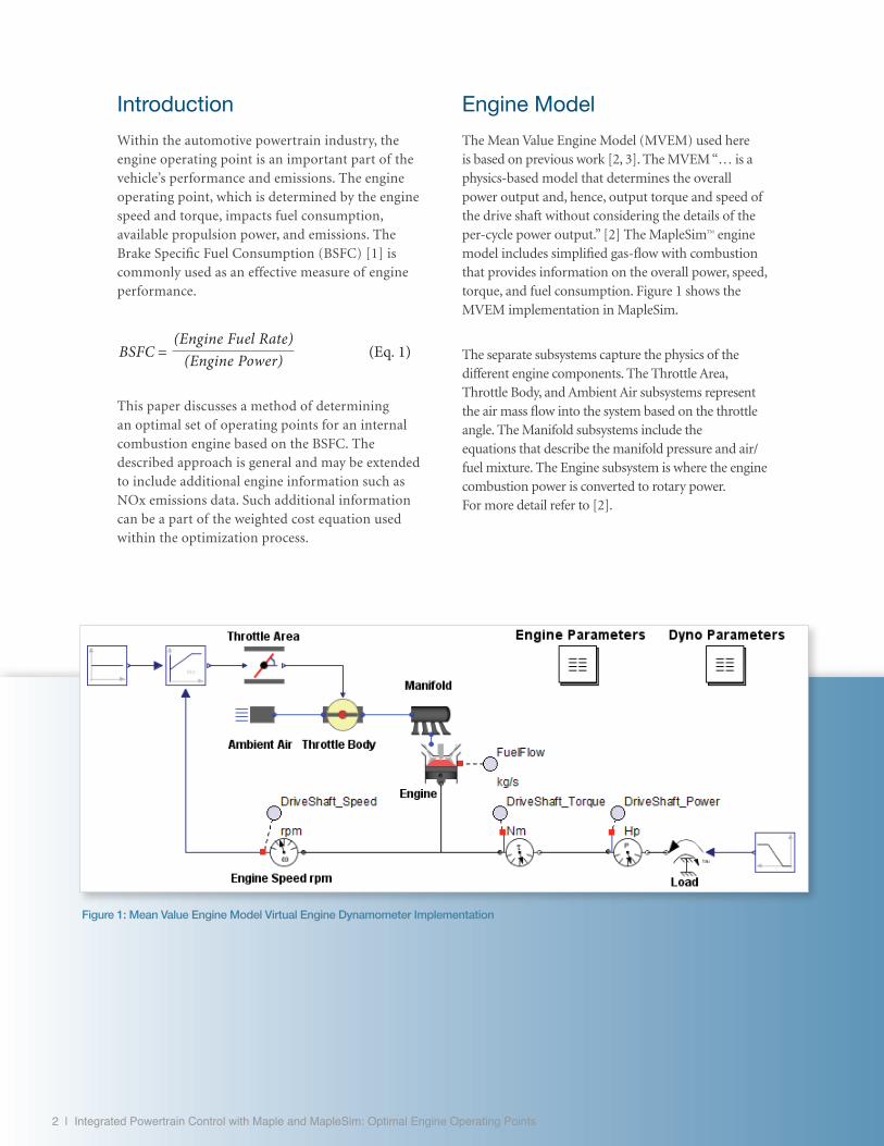
The Mean Value Engine Model (MVEM) used here is based on previous work [2, 3]. The MVEM “… is a physics-based model that determines the overall power output and, hence, output torque and speed of the drive shaft without considering the details of the per-cycle power output.” [2] The MapleSimTM engine model includes simplified gas-flow with combustion that provides information on the overall power, speed, torque, and fuel consumption. Figure 1 shows the MVEM implementation in MapleSim.

The separate subsystems capture the physics of the different engine components. The Throttle Area, Throttle Body, and Ambient Air subsystems represent the air mass flow into the system based on the throttle angle. The Manifold subsystems include the equations that describe the manifold pressure and air/fuel mixture. The Engine subsystem is where the engine combustion power is converted to rotary power. For more detail refer to [2].

Figure 1: Mean Value Engine Model Virtual Engine Dynamometer Implementation

P = τ n (Eq. 2)τ = f (n) (Eq. 3)

BSFC =(Engine Fuel Rate)

(Engine Power) (Eq. 1)

Virtual Engine Dynamometer Testing in MapleSim

In this work, the MVEM provides the average behavior of an internal combustion engine. The MVEM is combined with a virtual dynamometer test bench created in MapleSim for the engine testing. The MVEM is controlled by regulating the throttle to allow the engine to operate at equilibrium, set by the load torque and engine speed at which point the BSFC information is recorded. Figure 1 shows the MapleSim model of the virtual engine dynamometer simulation.

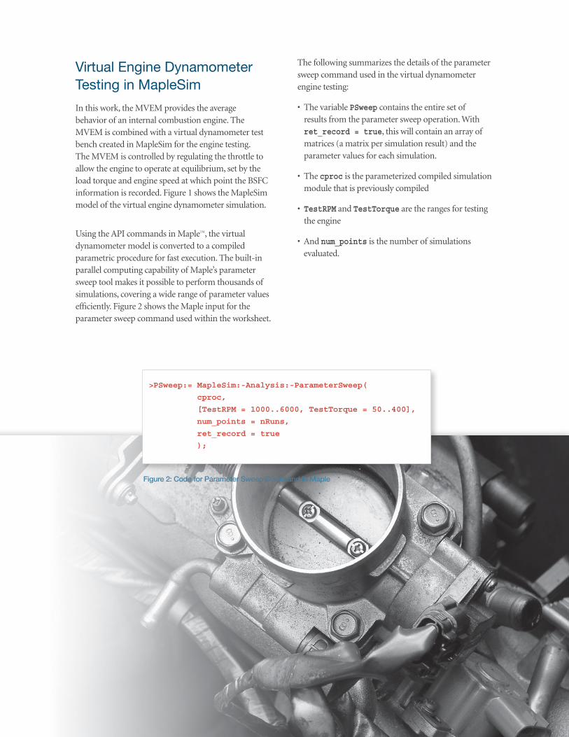
Using the API commands in MapleTM, the virtual dynamometer model is converted to a compiled parametric procedure for fast execution. The built-in parallel computing capability of Maple’s parameter sweep tool makes it possible to perform thousands of simulations, covering a wide range of parameter values efficiently. Figure 2 shows the Maple input for the parameter sweep command used within the worksheet.

The following summarizes the details of the parameter sweep command used in the virtual dynamometer engine testing:

• The variable PSweep contains the entire set of results from the parameter sweep operation. With ret_record = true, this will contain an array of matrices (a matrix per simulation result) and the parameter values for each simulation.

• The cproc is the parameterized compiled simulation module that is previously compiled

• TestRPM and TestTorque are the ranges for testing the engine

• And num_points is the number of simulations evaluated.

Figure 2: Code for Parameter Sweep Command in Maple

>PSweep:= MapleSim:-Analysis:-ParameterSweep(

cproc,

[TestRPM = 1000..6000, TestTorque = 50..400],

num_points = nRuns,

ret_record = true

);

Parameter Sweep Results

The raw data for the BSFC obtained from the parameter sweep runs is shown in Figure 3. The results include set-points where the engine was not able to achieve the desired equilibrium point as the torque load caused the engine to stall. This data can be discarded as the results are beyond the wide open throttle position for the engine and will need to be considered as unusable data for the engine map.

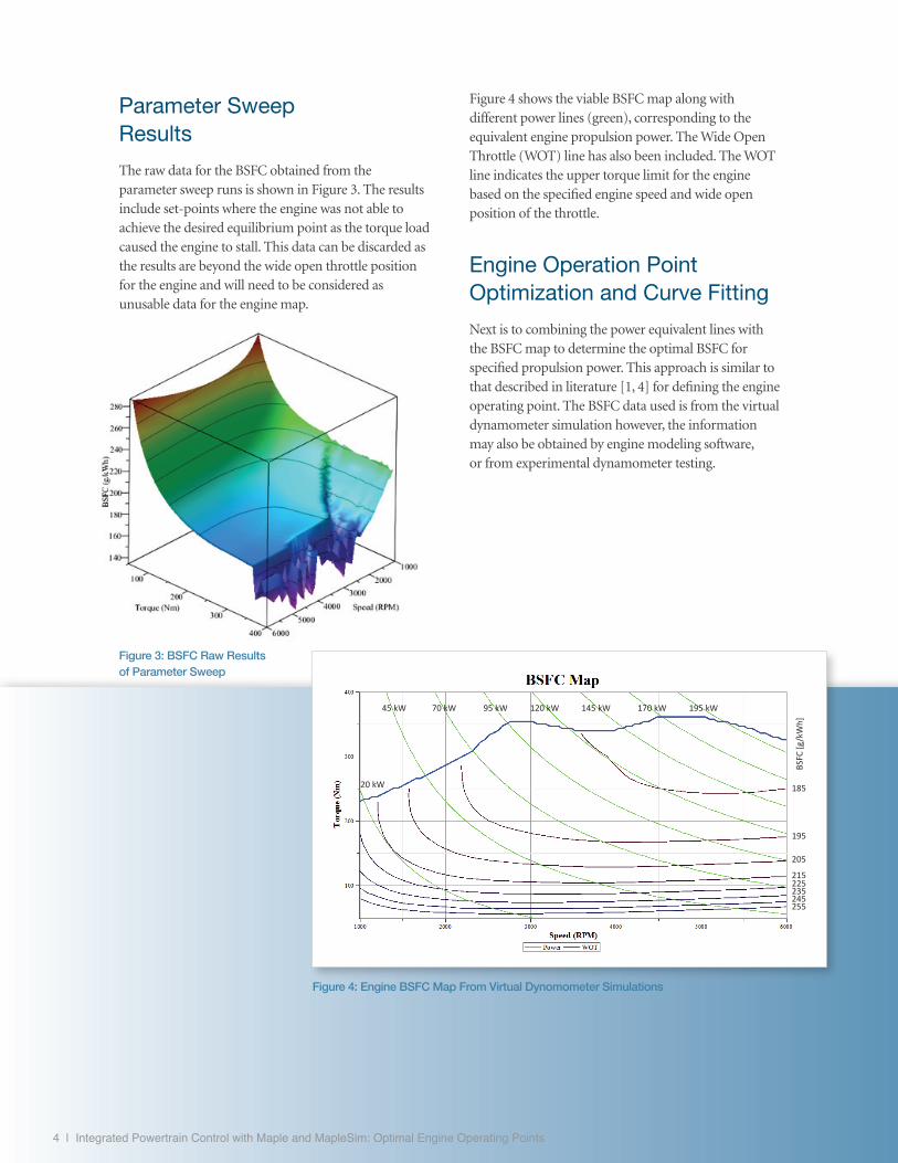
Figure 4 shows the viable BSFC map along with different power lines (green), corresponding to the equivalent engine propulsion power. The Wide Open Throttle (WOT) line has also been included. The WOT line indicates the upper torque limit for the engine based on the specified engine speed and wide open position of the throttle.

Engine Operation Point Optimization and Curve Fitting

Next is to combining the power equivalent lines with the BSFC map to determine the optimal BSFC for specified propulsion power. This approach is similar to that described in literature [1, 4] for defining the engine operating point. The BSFC data used is from the virtual dynamometer simulation however, the information may also be obtained by engine modeling software, or from experimental dynamometer testing.

4 | Integrated Powertrain Control with Maple and MapleSim: Optimal Engine Operating Points

185

195

205

215225235245255

195 kW170 kW145 kW120 kW95 kW70 kW45 kW

20 kWBS

FC [g

/kW

h]

Figure 4: Engine BSFC Map From Virtual Dynomometer Simulations

Figure 3: BSFC Raw Results of Parameter Sweep

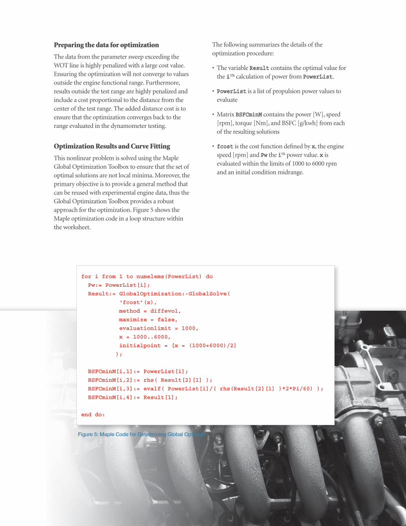
Preparing the data for optimization

The data from the parameter sweep exceeding the WOT line is highly penalized with a large cost value. Ensuring the optimization will not converge to values outside the engine functional range. Furthermore, results outside the test range are highly penalized and include a cost proportional to the distance from the center of the test range. The added distance cost is to ensure that the optimization converges back to the range evaluated in the dynamometer testing.

Optimization Results and Curve Fitting

This nonlinear problem is solved using the Maple Global Optimization Toolbox to ensure that the set of optimal solutions are not local minima. Moreover, the primary objective is to provide a general method that can be reused with experimental engine data, thus the Global Optimization Toolbox provides a robust approach for the optimization. Figure 5 shows the Maple optimization code in a loop structure within the worksheet.

The following summarizes the details of the optimization procedure:

• The variable Result contains the optimal value for the ith calculation of power from PowerList.

• PowerList is a list of propulsion power values to evaluate

• Matrix BSFCminM contains the power [W], speed [rpm], torque [Nm], and BSFC [g/kwh] from each of the resulting solutions

• fcost is the cost function defined by x, the engine speed [rpm] and Pw the ith power value. x is evaluated within the limits of 1000 to 6000 rpm and an initial condition midrange.

Figure 5: Maple Code for Determining Global Optimum

for i from 1 to numelems(PowerList) do

Pw:= PowerList[i];

Result:= GlobalOptimization:-GlobalSolve(

‘fcost’(x),

method = diffevol,

maximize = false,

evaluationlimit = 1000,

x = 1000..6000,

initialpoint = [x = (1000+6000)/2]

);

BSFCminM[i,1]:= PowerList[i];

BSFCminM[i,2]:= rhs( Result[2][1] );

BSFCminM[i,3]:= evalf( PowerList[i]/( rhs(Result[2][1] )*2*Pi/60) );

BSFCminM[i,4]:= Result[1];

end do:

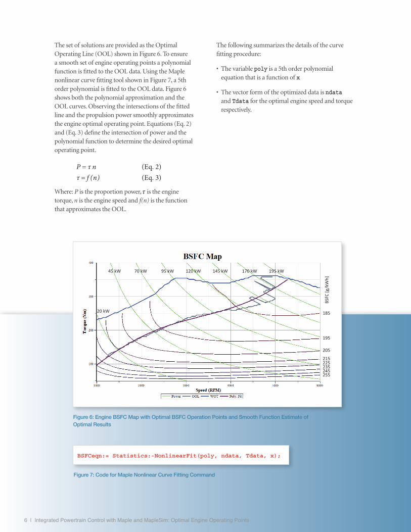
The set of solutions are provided as the Optimal Operating Line (OOL) shown in Figure 6. To ensure a smooth set of engine operating points a polynomial function is fitted to the OOL data. Using the Maple nonlinear curve fitting tool shown in Figure 7, a 5th order polynomial is fitted to the OOL data. Figure 6 shows both the polynomial approximation and the OOL curves. Observing the intersections of the fitted line and the propulsion power smoothly approximates the engine optimal operating point. Equations (Eq. 2) and (Eq. 3) define the intersection of power and the polynomial function to determine the desired optimal operating point.

Where: P is the proportion power, is the engine torque, n is the engine speed and f(n) is the function that approximates the OOL.

The following summarizes the details of the curve fitting procedure:

• The variable poly is a 5th order polynomial equation that is a function of x

• The vector form of the optimized data is ndata and Tdata for the optimal engine speed and torque respectively.

P = τ n (Eq. 2)τ = f (n) (Eq. 3)

BSFC =(Engine Fuel Rate)

(Engine Power) (Eq. 1)

6 | Integrated Powertrain Control with Maple and MapleSim: Optimal Engine Operating Points

195 kW170 kW145 kW120 kW95 kW70 kW45 kW

20 kW

BSFC

[g/k

Wh]

185

195

205

215225235245255

Figure 6: Engine BSFC Map with Optimal BSFC Operation Points and Smooth Function Estimate of Optimal Results

P = τ n (Eq. 2)τ = f (n) (Eq. 3)

BSFC =(Engine Fuel Rate)

(Engine Power) (Eq. 1)

BSFCeqn:= Statistics:-NonlinearFit(poly, ndata, Tdata, x);

Figure 7: Code for Maple Nonlinear Curve Fitting Command

Conclusion

By using Maple and MapleSim, complex engineering modeling and dynamic problems are effectively captured, modeled, and built-on. The concept presented extends the Mean Value Engine Model (MVEM) [2, 3]. Using the Brake Specific Fuel Consumption (BSFC) as the defining constraint, optimal operating points are determined for an internal combustion engine. The process describes the virtual dynamometer testing, BSFC engine map, optimization of engine data, followed by a function approximation of the optimal values. The function approximation of optimal dataset now serves as a target operating point for the internal combustion engine. Hence, allowing the engine to operate at the most effective fuel to power ratio defined by the BSFC. This paper focuses on the general approach and the technique may include additional engine characteristic such as emissions data in the optimization.

References

[1] S. Bai, J. Maguire and H. Peng, Dynamic Analysis and Control System Design of Automatic Transmissions, Warrendale, Pennsylvania, USA: SAE International, 2013.

[2] P. Goossens and A. Goodarzi, “Full-Vehicle Model Development For Prediction of Fuel Consumption”, SAE Int. J. Fuels Lubr., 2013.

[3] M. Saeedi, “A Mean Value Internal Combustion Engine Model in MapleSim”, M.A.Sc. thesis, Mech. Eng., Waterloo, Canada: University of Waterloo, 2010.

[4] J. V. Baalen, “Optimal Energy Management Strategy for the Honda Civic IMA”, Master’s thesis, Mech. Eng., Eindhoven: Technische Universiteit Eindhoven, 2006.

www.maplesoft.com | info@maplesoft.com© Maplesoft, a division of Waterloo Maple Inc., 2014. Maplesoft, Maple, and MapleSim are trademarks of Waterloo Maple Inc.

All other trademarks are the property of their respective owners.

A C y b e r n e t G r o u p C o m p a n y