integrated application of the cumulative score control chart and

Statistica Sinica 8(1998), 239-252

INTEGRATED APPLICATION OF THE CUMULATIVE

SCORE CONTROL CHART

AND ENGINEERING PROCESS CONTROL

Y. Eric Shao

Fu Jen Catholic University

Abstract: Recent years have witnessed heightened interest in the integration of sta-

tistical process control (SPC) and engineering process control (EPC). The present

study considers the utilization of the cumulative score (Cuscore) technique as an

interface between SPC and EPC in cases where a closed loop control is used for

process adjustment. Specifically, this study presents a scheme for the integrated

use of the Cuscore control chart with the minimum mean squared error (MMSE)

control. This study demonstrates the viability and potential advantages of this

scheme for combining SPC and EPC.

Key words and phrases: Cumulative score control chart, EPC, integration, mini-

mum mean squared error.

1. Introduction

Industrial quality engineers and control engineers have embraced divergentstrategies to reduce the variability of manufacturing processes and to maintaintargeted quality characteristics. Quality engineers have employed statistical pro-cess control (SPC) techniques (e.g., Shewhart control charts) to monitor the un-derlying process, whereas control engineers have utilized engineering process con-trol (EPC) techniques (e.g., Proportional-Integral-Differential control scheme) toregulate the process. Though the objective of both SPC and EPC is to reducethe variability of the process, the techniques differ substantially in approach.

Under Statistical Process Control (SPC), the results of an industrial process–anything from automobile assembly to pesticide production–may be representedas an ongoing series of data points plotted on any number of statistical controlcharts. A sound process should ideally generate independently and identicallydistributed (IID) random variables. However, fluctuations in this pattern mayarise even when a state of statistical control is achieved. Such disturbances arereflected as irregular sequences of observations (runs that are above or below acertain level) recorded on statistical control charts. When process outputs deviatesubstantially from the target–when the most recently plotted point falls beyondspecified bounds on the statistical control chart–an “alarm” is triggered. In such

240 Y. ERIC SHAO

situations, quality control engineers seek to identify and eliminate the causes.Thus Hess (1989) suggests that SPC be regarded as an “open loop advisor”.

However, these statistical control charts presuppose the statistical indepen-dence of each output observation. This assumption of independence demands astrict level of statistical control rarely achieved in practice. In reality, variousfactors–ranging from the continued presence of inertial elements to the results offrequent sampling–result in the serial correlation of process observations. Thisserial correlation skews the data reported on SPC charts and can increase the fre-quency of “false alarms”. Consequently, the in-control average run length (ARL)of the control charts would be much shorter than anticipated. The assumptionthat observations are independent is a significant handicap for SPC techniques.

In fact, the presence of autocorrelation (remains in observations) is some-times an indication that an EPC scheme is needed. A well tuned EPC should beable to produce uncorrelated data as the output deviation from target. EPC doesnot seek to isolate and eliminate the causes of departures from the target; EPC isdesigned, instead, to compensate for disturbances in the process by continuouslyadjusting the process. Though EPC can mitigate the effects of disturbances,EPC can rarely succeed in fully compensating for significant disruptions of theindustrial process. Consequently, the process mean (or variability) may driftconsiderably off target.

The present study aims to develop a technique which effectively fuses SPCand EPC so that the system is able to detect the presence of the transient dis-turbances in a process. A closed loop control will be discussed in this study.Although the Shewhart and cumulative sum (Cusum) control charts are welldeveloped and are widely used in industry, they have some limitations. For ex-ample, Montgomery (1996, p.314 and p.325) reported that Shewhart charts arenot sensitive to minor shifts in the process and that Cusum charts respond slowlyto large process shifts. Instead, Shao (1993) has found that the Cuscore controlchart is effective not only in detecting process shifts, but also in identifying tran-sient disturbances. The present study further demonstrates and evaluates theeffective integration of SPC and EPC through use of the Cuscore control chart.

2. Relevant Works

Widespread recognition of the enormous potential for enhanced quality andefficiency has fueled recent interest in the integration of SPC and EPC. Boxand Kramer (1992) provided an excellent examination of the interface betweenstatistical process monitoring and engineering feedback control and a thoroughcomparison of statistical process control and automatic process control (APC).Vandel Wiel, Tucker, Faltin and Doganaksoy (1992) proposed the algorithmic

INTEGRATED APPLICATION OF THE CUMULATIVE SCORE CONTROL CHART 241

statistical process control (ASPC) as a method of reducing predictable varia-tion; ASPC employs both feedback and feedforward control, and then monitorsthe system to detect and remove the assignable causes of disturbances. Hunter(1986) and Montgomery and Mastrangelo (1991) reported that the exponentiallyweighted moving average (EWMA) approach is equivalent to the Proportional-Integral-Differential (PID) control technique. However, MacGregor (1991) con-tended that the EWMA approach and PID control differ substantially. Mac-Gregor (1992) noted that because the level of the process output variable wouldbe a constant under the assumption of most control charts, the process shouldbe left alone unless a disturbance arising from an assignable cause is detected.Tucker (1992) also argued that control rules will compensate for assignable vari-ation if assignable cause variation could be predictable; when assignable causevariation is unpredictable, a search for assignable causes must be made. VanderWiel and Vardeman (1992) indicated that Cuscore charts can be developed toquickly signal the process level shifts, additive or innovational outliers, changesin model parameters, and other fluctuations in the process. Wardrop and Garcia(1992) highlighted the difficulty of designing an appropriate model for processdisturbances, which may assume a variety of forms (step change or linear changedisturbances), stem from a variety of causes, and enter the process at randomtimes. Their survey of various cases suggested that these disturbances cannotbe removed in many circumstances. Alwan and Roberts (1989), Montgomeryand Friedman (1989), and Montgomery and Mastrangelo (1991) have all rec-ommended that, whenever observations are autocorrelated, an appropriate timeseries model should be fitted to these observations and control charts then appliedto the residuals of the model.

Montgomery, Keats, Runger, and Messina (1994) examined the benefits ofcombining SPC and EPC techniques. Their simulations demonstrated the supe-riority of integrated use of SPC and EPC to the use of EPC alone. But whiletheir simulations employed the Shewhart, Cusum and EWMA control charts,the present study focuses upon a recently developed control chart–the Cuscorecontrol chart.

3. Cuscore Control Chart

Box and Ramirez (1992) provided a thorough introduction to the Cuscorecontrol chart. Consider a model which can be written as

at = f(yt, xt,m), t = 1, 2, . . . , n, (1)

where yt is the output observation, xt is the independent variable, m is an un-known parameter, and f() is some function. If m is the true value of the unknown

242 Y. ERIC SHAO

parameter, then the resulting at’s would follow a white noise sequence. Apartfrom a constant, the log likelihood for m = m0 is

l(m) = − 12σ2

n∑t=1

a2t0 ,

where the a2t0 ’s are obtained by setting m = m0 in Equation (1). Let −∂at

∂m

∣∣∣m−m0

= gt0 ; then the following relationship holds:

∂l(m)∂m

=1σ2

n∑t=1

at0gt0 .

The Cuscore statistic with the parameter value m = m0 is defined as:

Q0 =n∑

t=1

at0gt0 . (2)

Box and Ramirez (1992) demonstrated that the following relationship holds ifthe model is linear in parameter m and is approximate otherwise:

at0 = k(m − m0)gt0 + at. (3)

Equation (3) implies that an increase in discrepancy vector gt0 would be addedto at as long as the parameter m does not equal m0. This results in a sequen-tial correlation of at0 with gt0 . Consequently, the Cuscore statistic defined inEquation (2) would be continuously searching for the presence of the specificdiscrepancy vector. In addition, the least square estimator of (m − m0) as de-rived from Equation (3) would be m − m0 =

∑at0gt0/

∑g2t0 . This results in

Q = (m−m0)∑

g2t0 . Thus, when plotted against n, the Cuscore statistic should

be expected to provide a sensitive check for fluctuations in parameter m. As withthe Cusum control chart, changes in the slope of the Cuscore statistics may beused to detect the assignable causes of process shifts and disturbances.

Box and Ramirez (1992) presented the centred Cuscore (CC), the Cuscoreevaluated at m = m = (m0 + m1)/2. The CC is defined as:

CC =n∑

t=1

atgt,

where at = at(m) and gt = gt(m). They noted that the construction of controllimits with a Cuscore control chart would be equivalent to a series of Waldsequential tests (Wald (1947)) with boundaries (0,H). That is, if β (type II error)is negligible and can be ignored, then H = σ2 ln(1/α)/δ, where δ = m1 − m0.


Therefore, to detect changes in parameter m, control limits may be determined byplotting centred Cuscore statistics (which are evaluated at (m0 + m1)/2) againstn. That is,

UCL (upper control limit) =σ2 ln(1/α)

δ+when m1 > m0

LCL (lower control limit) =σ2 ln(1/α)

δ−when m1 < m0,

where δ+ = m1 − m0 (when m1 > m0) and δ− = m1 − m0 (when m1 < m0).

4. Cuscore Control Chart for a Closed Loop Control

4.1. Transient disturbances

Manufacturing process control seeks to minimize the deviation of the processoutput from the target quality characteristic and to minimize the process vari-ability as a means to enhance and maintain the quality of the finished product.However, industrial processes are frequently disturbed by unforeseen incidentsand by deliberate adjustments to the process. Changes in product design (shortproduction runs), vacillations in material properties (such as chemical impuri-ties), or unanticipated events (power or equipment failure) may all upset theproduction process and demand correction. These disruptions may all be con-sidered transient disturbances.

Transient disturbances typically fall into one of two categories: (1) stepchange disturbances and (2) linear change disturbances (or ramps). Step changedisturbances may result from adjustments in the process target; linear changedisturbances (LCD) may result from wearing out of a tool.

MacGregor, Harris, and Wright (1984) and Shao, Haddock, Runger, andWallace (1993) have examined transient models which represent step change dis-turbances as (1) (1−B)Dt = βt and linear change disturbances as (2) (1−B)(1−B)Dt = βt, where

B: Backward shift operator (e.g., B2Dt = Dt−2.)Dt: The transient disturbances at time t, and we assume that Dt would follow

either step or linear changes disturbances.βt: A random variable, and βt would be zero most of the time except when the

transient disturbances have occurred.

4.2. Step change transient disturbance with Cuscore control chart

According to MacGregor (1988), when the noise of the zero order systemfollows IMA (1,1) process, the minimum mean squared error (MMSE) controller

244 Y. ERIC SHAO

should behave as an integral controller. Similarly, when the noise of the first-order system follows the IMA (1,1) process, the MMSE controller should behaveas a proportional-integral (PI) controller. In addition, since the integral andPI controllers are widely used in industry, this study uses the MMSE (which isequivalent to integral or PI) control mode for feedback control action in the closedloop control. Appendix A shows that when a step-change disturbance enters theprocess, the output deviation would be yt+i = Dθi−1 + at+i. Therefore, after thetransient disturbance has been generated, the process may be described as:

yt = Dθt−1 + at.

In order to employ the Cuscore control chart, the above relationship could bereconstructed as yt = mDθt−1 + at. Therefore, at = yt − mDθt−1, and gt0 =−∂at

∂m |m−m0 = Dθt−1, at0 = (m − m0)gt0 + at = yt. The Cuscore statistic, thus,would be

Q0 =n∑

t=1

at0gt0 =n∑

t=1

ytD(θt−1).

4.3. Linear change transient disturbance with Cuscore control chart

In the case of the linear change transient disturbance, Appendix B shows thatthe output deviation would be yt+i = b(θi−1

θ−1 )+at+i. Therefore, after the transientdisturbance has been generated, one can represent the process as: yt = b(θt−1

θ−1 )+at. To use the Cuscore control chart, this relationship could be reconstructed asyt = mb(θt−1

θ−1 ) + at. Therefore, at = yt − mb(θt−1θ−1 ), and

gt0 = −∂at

∂m

∣∣∣m−m0

= b(θt − 1

θ − 1

), at0 = (m − m0)gt0 + at = yt.

The Cuscore statistic, thus, would be

Q0 =n∑

t=1

at0gt0 =n∑

t=1

ytb(θt − 1

θ − 1

). (4)

However, since the MMSE control action cannot completely compensate forthe linear change transient disturbance, the centred Cuscore’s ability to detect theassignable causes of transient disturbances attracts considerable interest. Con-sider a linear change disturbance with slope b = 1 (i.e., trend per period is ofmagnitude unity). The value of m0 is thus equal to 0, m1 is equal to 1 andm = (m0 + m1)/2 = 0.5. The CC is then obtained as the following:

CCt =n∑

t=1

atgt =n∑

t=1

[yt − 0.5b

(θt − 1θ − 1

)][b(θt − 1

θ − 1

)]. (5)


5. Simulation Studies

5.1. Use of Cuscore control chart

The performance of the Cuscore control chart may be illustrated throughsimulation of a process upset by a linear change disturbance. Specifically, thisstudy examined simulations of a zero-order process (both with and without en-gineering process control) in which a linear change disturbance with slope 1 isintroduced after observation 201 in a series of 400 observations. The value of pa-rameters q = 0.8 and θ = 0.5 are arbitrarily selected (however, they are typicalof those encountered in practice). The white noise follows a normal distributionwith mean 0 and standard deviation 1.

Figure 1 displays the process output deviations from target in the absence ofengineering process controls; after observation 201, the linear change disturbancepersists unabated for the duration of the process. Figure 2 shows the output de-viations from target after the integral control (i.e., Equation (A.1)) is introducedto tune the process. The integral control (which is equivalent to MMSE) partiallycompensates for the linear change disturbance, but it fails to return the processoutputs to target. Figure 3 plots both the Cuscore (defined as Equation (4)) andthe CC statistic (defined as Equation (5)) against time. The linear increase inthe Cuscore statistic values following observation 201 reflect the linear changedisturbance. A CC value falling beyond an upper or lower bound would signalthe presence of a linear change disturbance. For example, H would be equal to4.61 with α(type I error)= 0.01. Thus, according to Figure 3, an out of controlalarm due to the assignable causes may be expected at time 203.

Outp

ut

devia

tions

Observation Number, t

Figure 1. Output deviations from target (without use of EPC). A lineardisturbance starts at t = 201.

246 Y. ERIC SHAO

Outp

ut

devia

tions


Figure 2. Output deviations from target (with use of MMSE control). Alinear disturbance starts at t = 201.

Cuscore

CC

H


Figure 3. Plot of Cuscore and Centred Cuscore statistics. An out-of-controlsignal is given at t = 203.

This simulation assumed that the period needed to identify and eliminatethe assignable cause of the linear change disturbance was 10 times unity from thepoint of initial detection by the Cuscore control chart. Thus, in this simulation,the disturbance was detected at time 203 and terminated at time 212. Figure4 plots output deviations from target after the Cuscore control chart is applied,and it shows that the linear change disturbance is compensated by employingthe integration of Cuscore control chart and MMSE control.


Outp

uts

devia

tions

(EP

C/C

usc

ore

)


Figure 4. Output deviations from target (with use of MMSE/Cuscore). Alinear disturbance starts at t = 201.

5.2. Performance of Cuscore control chart in comparison

The first simulation demonstrated the effectiveness of the Cuscore controlchart as a tool for integrating SPC and EPC. As a supplementary consideration,a second comprehensive simulation was conducted to compare the performanceof the Cuscore control chart with the performance of other SPC techniques inintegrated EPC/SPC schemes.

As in the previous simulation, this simulation examines zero-order processes(both with and without engineering process control), with parameter values ofq = 0.8 and θ = 0.5, in which a linear change disturbance is introduced afterobservation 201 in a series of 400 observations. The performance measure (PM)applied is the average squared deviation from the target (T). That is, PM =1/n

∑nt=1(yt − T )2.

In Figure 1, with no EPC (i.e., integral control) action, PM = 7103.292; inFigure 2 with applying integral control action, PM = 3.0805. This simulationalso assumes that the linear change disturbance results from the assignable cause,and that the magnitudes of the trend are 0.1, 0.5, 1.0, 1.5, and 2.0 units perperiod. As in the previous simulation, the assignable cause occurs at time 201and the period needed to identify and eliminate the assignable cause is 10 timesunity once detected.

Three different SPC control charts for the output deviation from target wereexamined: a Shewhart chart for individuals with 3σ control limits, a Cusumchart with k = 0.5 and h = 5, and a Cuscore chart with H = 4.61. Thevalues of k = 0.5 and h = 5 for the Cusum chart were selected because they

248 Y. ERIC SHAO

are effective across a broad range of process shifts (Montgomery, Keats, Runger,and Messina (1994)). Performance measures are computed across 400 periodsfor 1000 simulation runs; likewise, the integral control action is employed for all400 periods of 1000 simulation runs.

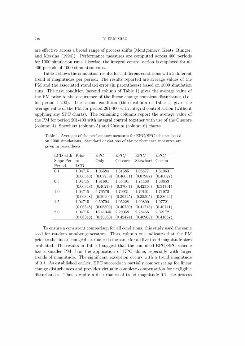
Table 1 shows the simulation results for 5 different conditions with 5 differenttrend of magnitudes per period. The results reported are average values of thePM and the associated standard error (in parentheses) based on 1000 simulationruns. The first condition (second column of Table 1) gives the average value ofthe PM prior to the occurrence of the linear change transient disturbance (i.e.,for period 1-200). The second condition (third column of Table 1) gives theaverage value of the PM for period 201-400 with integral control action (withoutapplying any SPC charts). The remaining columns report the average value ofthe PM for period 201-400 with integral control together with use of the Cuscore(column 4), Shewhart (column 5) and Cusum (column 6) charts.

Table 1. Averages of the performance measures for EPC/SPC schemes basedon 1000 simulations. Standard deviations of the performance measures aregiven in parenthesis.

LCD with Prior EPC EPC/ EPC/ EPC/Slope Per to Only Cuscore Shewhart CusumPeriod LCD0.1 1.04715 1.06584 1.31585 1.06677 1.51963

(0.06348) (0.07259) (0.46651) (0.07987) (0.40027)0.5 1.04715 1.91691 1.55491 1.74468 1.53653

(0.06348) (0.40273) (0.37007) (0.42350) (0.34791)1.0 1.04715 4.76576 1.70931 1.79161 1.71972

(0.06348) (0.20206) (0.39225) (0.35505) (0.38624)1.5 1.04715 9.59794 1.95228 1.99800 1.97721

(0.06348) (0.08809) (0.40750) (0.41713) (0.40741)2.0 1.04715 16.41345 2.29058 2.28466 2.32172

(0.06348) (0.35560) (0.42474) (0.40908) (0.41667)

To ensure a consistent comparison for all conditions, this study used the sameseed for random number generators. Thus, column one indicates that the PMprior to the linear change disturbance is the same for all five trend magnitude sizesevaluated. The results in Table 1 suggest that the combined EPC/SPC schemehas a smaller PM than the application of EPC alone, especially with largertrends of magnitude. The significant exception occurs with a trend magnitudeof 0.1. As established earlier, EPC succeeds in partially compensating for linearchange disturbances and provides virtually complete compensation for negligibledisturbances. Thus, despite a disturbance of trend magnitude 0.1, the process


operating with EPC alone acts as if there is no linear change disturbance for theperiod of 201-400.

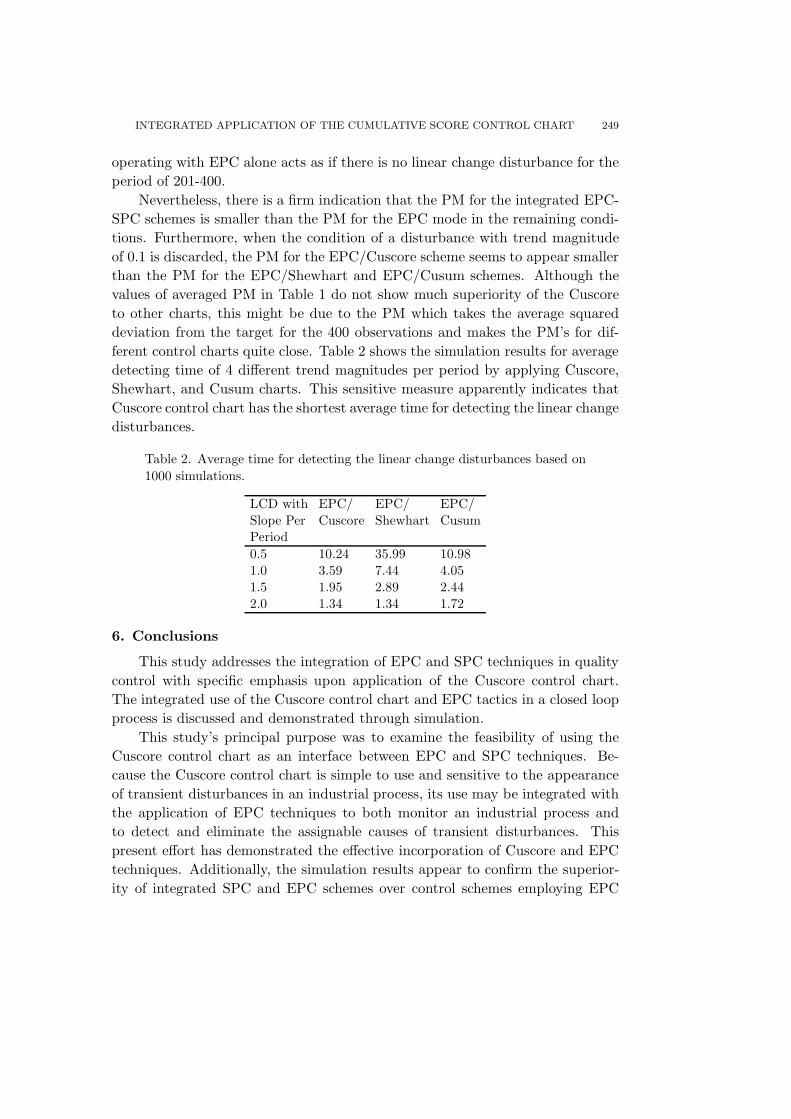
Nevertheless, there is a firm indication that the PM for the integrated EPC-SPC schemes is smaller than the PM for the EPC mode in the remaining condi-tions. Furthermore, when the condition of a disturbance with trend magnitudeof 0.1 is discarded, the PM for the EPC/Cuscore scheme seems to appear smallerthan the PM for the EPC/Shewhart and EPC/Cusum schemes. Although thevalues of averaged PM in Table 1 do not show much superiority of the Cuscoreto other charts, this might be due to the PM which takes the average squareddeviation from the target for the 400 observations and makes the PM’s for dif-ferent control charts quite close. Table 2 shows the simulation results for averagedetecting time of 4 different trend magnitudes per period by applying Cuscore,Shewhart, and Cusum charts. This sensitive measure apparently indicates thatCuscore control chart has the shortest average time for detecting the linear changedisturbances.

Table 2. Average time for detecting the linear change disturbances based on1000 simulations.

LCD with EPC/ EPC/ EPC/Slope Per Cuscore Shewhart CusumPeriod0.5 10.24 35.99 10.981.0 3.59 7.44 4.051.5 1.95 2.89 2.442.0 1.34 1.34 1.72

6. Conclusions

This study addresses the integration of EPC and SPC techniques in qualitycontrol with specific emphasis upon application of the Cuscore control chart.The integrated use of the Cuscore control chart and EPC tactics in a closed loopprocess is discussed and demonstrated through simulation.

This study’s principal purpose was to examine the feasibility of using theCuscore control chart as an interface between EPC and SPC techniques. Be-cause the Cuscore control chart is simple to use and sensitive to the appearanceof transient disturbances in an industrial process, its use may be integrated withthe application of EPC techniques to both monitor an industrial process andto detect and eliminate the assignable causes of transient disturbances. Thispresent effort has demonstrated the effective incorporation of Cuscore and EPCtechniques. Additionally, the simulation results appear to confirm the superior-ity of integrated SPC and EPC schemes over control schemes employing EPC

250 Y. ERIC SHAO

alone in many circumstances and, furthermore, to suggest the superiority of Cus-core/EPC scheme to other SPC/EPC integrations in certain circumstances.

Acknowledgements

This research was supported in part by the National Science Council of theRepublic of China, Grant No. NSC 84-2121-M-030-003. The author would liketo thank the Chair Editor and the referees for several valuable comments.

Appendix A. Output Deviations Under Zero Order System with Inte-gral Control When Step Change Transient Disturbance Exists

The zero order system with noise of IMA(1,1) process could be modelled asyt+1 = qxt + dt+1, and dt+1 = (1−θB)at

(1−B) , where dt+1 is the noise at time t + 1and it follows IMA(1,1) process, yt+1 is the output deviation from target at timet + 1, and xt is control variable’s deviation from nominal value at time t. Theintegral (I) control action is (MacGregor (1988))

xt = −(1 − θ)q

t∑j=−∞

yj. (A.1)

Now, suppose the step change transient disturbance has started to affect theprocess at time t + 1, then the following consequences would happen.

(1) At time t + 1.Since the step change transient disturbance has started to affect the process attime t + 1, therefore the process should be represented as

yt+1 = qxt + dt+1 + Dt+1. (A.2)

Substituting Equation (A.1) into Equation (A.2), it can be shown that:

yt+1 = q[− (1 − θ)

q

t∑j=−∞

yj

]+ dt+1 + Dt+1

= Dt+1 + at+1

(since

t∑j=−∞

yj =at

(1 − B)

).

Therefore, the control action would be

xt+1 = xt − (1 − θ)q

Dt+1 − (1 − θ)q

at+1. (A.3)

(2) At time t + 2.


The underlying process should be represented as

yt+2 = qxt+1 + dt+2 + Dt+2. (A.4)

Substituting Equation (A.3) into Equation (A.4), it can be shown that: yt+2 =aa+2 + Dt+2 − (1 − θ)Dt+1. Therefore, the control action would be xt+1 =xt − (1−θ)

q yt+2. Continuing doing this way, we are able to conclude that

yt+i = Dt+i−(1−θ)Dt+i−1−(1−θ)θDt+i−2−(1−θ)θ2Dt+i−3+ · · ·+at+i, (A.5)

where i stands for the time when the transient disturbance started affecting theprocess. In the case of step change transient disturbance, the magnitude of thelevel is assumed to be D. Therefore, Dt+i = Dt+i−1 = Dt+i−2 = · · · = Dt+1 = D.Equation (A.5) can be rewritten as

yt+i = D[1 − (1 − θ)− (1 − θ)θ − · · · − (1 − θ)θi−2] + at+i

= D[1 − (1 − θ)(1 + θ + θ2 + · · · + θi−2)] + at+i.

Then, it can be shown that yt+i = Dθi−1 + at+i.

Appendix B. Output Deviations Under Zero Order System with Inte-gral Control When Linear Transient Disturbance Exists

In the case of linear transient disturbance, the disturbance can be reformedas Dt = a + bi, where a is the magnitude of the level and b is the slope. Supposea = 0 without lose generality, then Equation (A.5) can be reformed as

yt+i = b{i − (1 − θ)[(i − 1) + θ(i − 2) + θ2(i − 3) + · · · + θi−2]} + at+i.

It can be shown that yt+i = b(θi−1θ−1 ) + at+i.

References

Alwan, L. C. and Roberts, H. V. (1989). Time series modeling for statistical process control.

In Statistical Process Control in Automated Manufacturing (Edited by J. B. Keats and N.

F Hubele), 45-65. Marcel Dekker, New York.

Box, G. E. P. and Kramer, T. (1992). Statistical process monitoring and feedback adjustment-A

discussion. Technometrics 34, 251-285.

Box G. E. P. and Ramirez, J. (1992). Cumulative score charts. Quality and Reliability Engi-

neering International 10, 17-27.

Hess, J. H. (1989). Managing Quality. CHEMTECH 19, 412-416.

Hunter, J. S. (1986). The exponentially weighted moving average. Journal of Quality Technology

18, 203-210.

MacGregor, J. F., Harris, T. J. and Wright, J. D. (1984). Duality between the control of

processes subject to randomly occurring deterministic disturbances and ARIMA stochastic

disturbances. Technometrics 26, 389-397.

252 Y. ERIC SHAO

MacGregor, J. F. (1988). On-line statistical process control. Chemical Engineering Progress

21-31.

MacGregor, J. F. (1991). Discussion of “Some statistical process control methods for autocor-

related data”. Journal of Quality Technology 23, 198-199.

MacGregor, J. F (1992). Discussion of “Statistical process monitoring and feedback adjustment-

A discussion”. Technometrics 34, 273-275.

Montgomery, D. C. and Friedman, D. J. (1989). Statistical process control in a computer-

integrated manufacturing environment. In Statistical Process Control in Automated Man-

ufacturing (Edited by J. B. Keats and N. F. Hubele), 67-87. Marcel Dekker, New York.

Montgomery, D. C. (1996). Introduction to Statistical Quality Control, 3rd edition. John Wiley,

New York.

Montgomery D. C. and Mastrangelo, C. M. (1991). Some statistical process control methods

for autocorrelated data. Journal of Quality Technology 23, 179-204.

Montgomery D. C., Keats, J. B., Runger, G. C. and Messina, W. S. (1994). Integrating statis-

tical process control and engineering process control. Journal of Quality Technology 26,

79-87.

Shao, Y. E. (1993). A Real Time Stochastic Process Control System for Process Manufacturing.

Ph.D. Dissertation, Rensselaer Polytechnic Institute.

Shao, Y. E., Haddock, J., Runger, G. and Wallace, W. A. (1993). Controlling the transient

stage of a manufacturing process. Proceeding of the 2nd Industrial Engineering Research

Conference 739-743.

Tucker, W. T. (1992). Discussion of “Statistical process monitoring and feedback adjustment-A

discussion”. Technometrics 34, 275-277.

Vander Wiel, S., Tucker, W. T., Faltin, F. W. and Doganaksoy, N. (1992). Algorithmic statis-

tical process control: Concepts and an application. Technometrics 34, 286-297.

Vander Wiel, S. and Vardeman, S. B. (1992). Discussion of “Statistical process monitoring and

feedback adjustment-A discussion”. Technometrics 34, 278-281.

Wald, A. (1947). Sequential Analysis. Wiley, New York.

Wardrop, D. M. and Garcia, C. E (1992). Discussion of “Statistical process monitoring and

feedback adjustment-A discussion”. Technometrics 34, 281-282.

Institute of Applied Statistics and Departmant of Statistics, Fu Jen Catholic University, Taipei,

Taiwan.

E-mial: [email protected]

(Received September 1995; accepted December 1996)

integrated application of the cumulative score control chart and

Documents