Integrated Aeromechanics with Three-Dimensional

Solid-Multibody Structures

Anubhav Datta Wayne Johnson

Science and Technology Corp Aeromechanics Branch

AFDD at Ames Research Center NASA Ames Research Center

Moffett Field, CA 94035 Moffett Field, CA 94035

ABSTRACT

A full three-dimensional finite element-multibody structural dynamic solver is coupled to a three-dimensional Reynolds-averaged Navier-Stokes solver for the prediction of integrated aeromechanical stressesand strains on a rotor blade in forward flight. The objective is to lay the foundations of all major pieces of anintegrated three-dimensional rotor dynamic analysis — from model construction to aeromechanical solutionto stress/strain calculation. The primary focus is on the aeromechanical solution. Two types of three-dimensional CFD/CSD interfaces are constructed for this purpose with an emphasis on resolving errorsfrom geometry mis-match so that initial-stage approximate structural geometries can also be effectivelyanalyzed. A three-dimensional structural model is constructed as an approximation to a UH-60A-like fullyarticulated rotor. The aerodynamic model is identical to the UH-60A rotor. For preliminary validationmeasurements from a UH-60A high speed flight is used where CFD coupling is essential to capture theadvancing side tip transonic effects. The key conclusion is that an integrated aeromechanical analysis isindeed possible with three-dimensional structural dynamics but requires a careful description of its geometryand discretization of its parts.

INTRODUCTION

The objective of this paper is to lay the foundationsof an integrated three-dimensional (3D) aeromechanicalanalysis for helicopter rotors. The words “integrated3D aeromechanics” are used to mean three-dimensionalstructural dynamics coupled to three-dimensional fluiddynamics for the prediction of dynamic stresses andstrains with an equal fidelity of representation in struc-tures and fluids.

The state of the art in aeromechanical analysis usesReynolds Averaged Navier-Stokes (RANS) based Com-putational Fluid Dynamics (CFD) containing tens ofmillions of grid points on hundreds of cores, routinely,in a research environment for the rotor, and even forthe entire helicopter. Arbitrary blade contours, air-craft configurations, and flight conditions can be an-alyzed effectively from first principles. Computationsin the structural domain continue to use engineering-level beam-multibody models that are historically partof lifting-line comprehensive codes carried out on a sin-

Presented at the American Helicopter Society 70th AnnualForum, Montreal, Quebec, May 20–22, 2014. This is a work of theU.S. Government and is not subject to copyright protection.

gle processor [1]. Thus the high-fidelity CFD airloadsare not directly integrated with stress/strain calcula-tions. Similarly detailed finite element stress analysis isperformed routinely on structures but only on isolatedcomponents with loading from beam analysis or previ-ous flight test data. Thus high-fidelity structures is notintegrated with high-fidelity airloads. The need for high-fidelity structures for dynamics is clear. Modern rotorscontain flexible components near the hub that providethe critical couplings for dynamics and encounter thecritical stresses. These have short aspect ratios, opensections, and end constraints, and cannot be treated asbeams. Blades envisioned with advanced shapes and theability to morph in flight cannot be treated from firstprinciples using beams.

The broad objective of this research is to close thisgap by developing a scalable 3D solid-multibody basedComputational Structural Dynamics (CSD) solver. Theformulations for 3D scalability and multibody dynamicswere covered earlier in Refs [2] and [3]. The focus ofthis paper is on integrated aeromechanics. The specificobjectives are: 1. to develop a 3D CFD/CSD coupledsolution procedure and demonstrate it on a realistic ar-ticulated rotor and 2. to implement an entire 3D work-flow from model construction to aeromechanical solutionto stress/strain calculation.

1

Figure 1: Integrated 3D workflow.

The field of computational 3D fluid-structure inter-action is vast and varied (see recent reviews and texts[4]– [8]) but have never been applied in the context of ro-torcraft. Rotorcraft requires a special solution procedure— a straight forward exchange of states and accompa-nying iterations will not do. Rotor control angles mustbe simultaneously determined to satisfy the aircraft trimstate. Adequate aerodynamic damping must be providedto the structure as a pre-conditioner so that all classesof rotors can be solved. Theoretical considerations ofconservation and consistency are not sufficient, an effec-tive analysis must accommodate early-stage structuraldescriptions with significant geometry mis-match. Theseare the particular emphases of this paper.

The 3D structural model constructed for this workis an idealized representation of a fully articulated UH-60A-like rotor. Construction of exact geometries fromCAD and generation of 3D finite element-multibodymeshes is a separate dedicated effort in itself and de-scribed in a companion paper [9].

Scope and Organization of Paper

The main emphasis of this work is on the develop-ment and demonstration of an integrated 3D CFD/CSDanalysis capability. A complete capability demonstra-tion also requires all supporting pieces of a new work-flow to be covered. Many of these supporting pieces arecovered in an idealized manner. For example 3D geom-etry and meshing is a critical piece for such a capabilityyet dealt in a crude and coarse manner adequate onlyfor the purposes of capability demonstration. The com-parisons shown at the end between predictions and mea-surements are therefore not true validations but only abasis for qualitative verification. Nevertheless they pro-

vide the first glimpse of the kind of detailed stress/strainanalysis possible using integrated 3D aeromechanics.

The paper is organized as follows. Following intro-duction, the paper begins by describing the new work-flow. The next section describes the 3D CSD solver.The external CFD solver used for coupling is then brieflysummarized. The fourth section describes the construc-tion of 3D structural models. The fifth section coversthe 3D CFD/CSD formulation — interfaces (spatial cou-pling) and the solution procedure (temporal coupling).The final section presents results from a fully integrated3D analysis. The paper ends with some concluding ob-servations.

INTEGRATED 3D WORKFLOW

Integrated 3D analysis requires a new workflow.The key pieces of this workflow are envisioned in Fig 1.

The workflow begins with a CAD model. It canbe a gross description in the early stages of structuraldesign, then progressively refined and populated withdetails as the design advances. The CAD geometry isthen interpreted into a Structural Analysis Represen-tation (SAR) geometry by the dynamicist. The SARincludes only those parts considered necessary for anal-ysis and identifies them as a flexible part, a multibodypart, or a device part. Flexible parts are marked for3D meshing, multibody parts are assigned their func-tionality (joint type and constraints), and device partsare noted for special-purpose treatment. The flexibleparts are those with significant strains. The multibodyparts are idealizations of constraints that allow arbitrar-ily large relative motions between flexible parts. Devicesare special-purpose parts which allow off-line character-

2

istics to be included (e.g. look-up tables for a non-linearlag damper). The next task is to mesh the flexible parts.Once meshed, all parts are re-integrated into a Struc-tural Analysis Model (SAM) geometry. The SAM taskmerges all 3D parts, prescribes material properties, des-ignates constrained nodes for multibody connection, de-fines the matematical properties of all joints (rotation or-der, locked versus free states and command signals), de-fines the physical properties of all joints (stiffness, damp-ing, actuation force and ± free play), and completes theappropriate description of devices. The completed SAMis then ready for the CSD solver. All of these tasks fallunder the broad category of 3D geometry and meshing(a companion paper [9] is devoted to this category).

A CSD solver must be equipped with special capa-bilities for rotorcraft — a pure structural dynamic anal-ysis will not do. An internal aerodynamic module isneeded for efficient coupling with CFD. A trim module isneeded to achieve the mean rotor operating state. Theserequire a top level description of aircraft geometry andconfiguration. Trim requires integrated loads (inertialand aerodynamic) at the hub from multiple load pathsacross multiple parts for which a specialized hub loadsmodule is needed. A high-fidelity interface is needed for3D fluid-structure coupling. The solution procedure forcoupling is special and requires all of the above modules.All of these pieces are grouped within the broad cate-gory of a rotor dynamic solver. The 3D fluid-structureinterface piece is generic to any external CFD solver(with structured or unstructured surface mesh). TheCFD solver used in this work is part of the HPCMPCREATETM – AV Helios software. This required theCSD solver to be incorporated within the Helios envi-ronment. This environment is presently equipped to ex-ecute a CSD solver from only a single processor — as perrequirements of current generation comprehensive codes.While this is not a barrier for the main emphasis of thispaper it prevents the Structural Partitioning piece of theworkflow from implementation (Fig 1). It also preventsmeaningful timing conclusions to be drawn.

3D ROTOR DYNAMIC SOLVER

The 3D rotor dynamic solver consists of a core 3Dsolid-multibody CSD solver, an aircraft geometry mod-ule, an internal aerodynamics module, a hub loads mod-ule, a trim module and a 3D fluid-structure interfacemodule. The fluid-structure interface module is de-scribed in detail in a later section. The present workconsiders only an isolated rotor so the aircraft geometrymodule is not used. A brief summary of the rest areprovided below.

3D Solid-multibody CSD Solver. The flexible partsof a structure are solved by 3D governing equations ofmotion derived in a rotating frame (non-rotating is asimplification) using generalized Hamilton’s Principle.

The formulation uses Green-Lagrange strains and secondPiola-Kirchhoff stresses for strain energy and follows ageometrically exact nonlinear Total Lagrangian formu-lation. Exact geometry and strains are a pre-requisitefor unifying multibody dynamics within 3D. The stress-strain relationship is linear. Isoparametric, second or-der, brick elements: 27-node hexahedral elements and10-node tetrahedral elements are available for discretiza-tion of the structure. See Ref [2] for details.

The multibody connections and constraints use Eu-ler angle joints. A special formulation is used whichpreserves kinematic exactness between 3D elements un-dergoing arbitrary rotations relative each other while atthe same time eliminating all algebraic constraint equa-tions. The special formulation is a joint that is associ-ated with 12 states — 6 are interface states that con-strain the position and orientation of the joint in spaceand another 6 are the joint states that describe its de-formation. The joint states can be constrained (locked),commanded (prescribed) or actuated (forced). Connec-tions are also special in 3D — they represent true con-nections. Connection points must be identified preciselyon the flexible parts and a mesh generated with nodesavailable at those locations. If the connection points arenot known a priori a generic connection can be used thatconstrains an entire face of the flexible part. The inter-nal stresses at the edge will then be incorrect but thekinematic exactness will still be preserved. See Ref [3]for details.

Three classes of algebraic solvers are available: di-rect, iterative, and eigen. The direct solver is a skylinesolver. The iterative solvers are iterative-substructuringsolvers based on Finite Element Tearing and Intercon-necting - Dual Primal preconditioners and equipped withConjugate Gradient and Generalized Minimum Residualupdates. The eigen solvers are not developed as part ofthis work but available as calls to external scaLapackroutines [10]. The direct solver is most efficient on asingle processor but not parallel. The iterative solversare parallel and scalable and meant for large scale dis-tributed execution. The eigen solvers are parallel butnot scalable. Because the present environment restrictsthe solver to a single processor the direct solver is used.

The algebraic solvers are the building blocks ofstructural solvers. Two types of structural solvers areavailable, both employing a direct time integration ofthe second order nonlinear structural dynamic equations.The first is a single time-step Generalized-α Method [11]and the other is a two time-step trapezoidal plus three-point backward Euler combination [12]. The 3D solid-multibody models are strongly nonlinear and the dy-namic stiffness matrix must be updated at every timestep for accuracy of the response solution. Additionally,structural sub-iterations (Newton-Raphson) are possiblewithin both classes of solvers, but required only for rel-atively large time steps.

3

Internal Aerodynamics. The internal aerodynamicsmodel, presently, is only meant to support CFD cou-pling, hence elementary: quasi-steady linear aerodynam-ics with uniform inflow. Its purpose is to provide airloadsensitivities to blade deformations (aerodynamic damp-ing) so non-circulatory airloads are also required (for tor-sion damping). Aerodynamic angles (angle of attack αand sideslip β) are extracted from the 3D deformationfield using the deformed chord orientation relative airflow and blade velocities at 3/4 − c location (see sec-tion on 3D Structural Models) as per thin airfoil the-ory. Both angles and rates are required for the angleof attack. There is no aerodynamic damping in lag soeither a damper model is needed (a simple linear modelis used here) or artificial damping added and bled outconsistently to decay initial transients. Transients in lagdynamics make a direct integration in time to periodic-ity an expensive solution process. Even with the knowndamper value for this existing rotor about 15 revolutionsare needed to decay any lag transients.

Hub Loads. The root shears and moments in therotating frame are calculated either by force summationor from joint reactions. The counterpart of the deflec-tion method in beams is a direct stress integration in 3D.Stress integration is available for the flexible parts but atthe ends or at the joint connection points — where theintegrated loading is actually desired — 3D edge effectsor local concentration effects occur and contaminate thesolution. The effects are real but require a high localmesh resolution to capture. The contamination of globaltrim solution with local mesh resolution is considered un-acceptable. Thus force summation or joint reactions areneeded instead of the stress integration method. (Notethat even in beams shear forces cannot be resolved di-rectly — if at all — using deformations and a force sum-mation is always needed). These are needed also forelements that are idealized to be rigid. The force sum-mation method is same in principle as in beams exceptthat a volume integration is needed in 3D. For a con-verged response both should be identical (see section on3D CFD/CSD Analysis Results) even though in generalforce summation is more accurate for higher frequen-cies and larger time steps. Joint reactions are neededfor multiple load paths. Here joints are used as sensorswhich means they have to be assigned a small flexibilityin the direction (and type) of the desired loading. Thus,strictly, sensing alters the dynamic characteristics of themodel — but is not inconsistent with the real behaviorof systems.

Trim Solution. Once hub loads are obtained thetrim solution is straight forward. Presently only isolatedrotor options are available: wind tunnel trim (targets arethrust or coning and two cyclic flapping angles), momenttrim (targets are thrust or coning and two hub moments)and propulsive trim (targets are lift and propulsive forceand either two cyclic flapping angles or two hub mo-

ments). The control inputs are via joint commands (ad-ditionally shaft tilt for propulsive trim) imposed eitherat the blade root bearing or at the base of the pitch link.

3D CFD SOLVER

The CFD solver used is part of the HPCMPCREATETM – AV Helios software. It is an integratedcapability consisting of an unstructured, node-centered,implicit RANS (Spalart-Allmaras turbulence) near-bodysolver, an overset Cartesian, explicit, Euler off-bodysolver, and an implicit hole-cutting based domain con-nectivity algorithm. The solver has been extensively val-idated with current state of the art beam models for thesame rotor used in this paper. A description of its gen-eral architecture can be found in Ref [13]; validation ofits aerodynamic and CFD/CSD capabilities can be foundin Ref [14].

The aerodynamic set up is identical to Ref [14]. Acoarse mesh set-up is used. The near-body grid contains4.5 million points and extends up to 5.8 chords. Theoff-body grids contains about 14 million nodes (finestspacing of 0.18 chord) and extends up to 58 chords. Anazimuthal discretization of 0.25◦ is used with 25 sub-iterations for the near-body solver and a single sub-stepfor the off-body solver. The Courant-Friedrichs-Lewynumber for the off-body solver for this time step is 1.67.The CFD solver is executed on 128 processors.

3D STRUCTURAL MODELS

A four-bladed fully articulated rotor model is con-sidered. Each blade is an assembly of several flexible andjoint parts. The lag damper is not modeled as a sepa-rate device but included as a linear damper as part of ajoint. Two different configurations (baseline and simple)and two different blade meshes (baseline and simple) areconstructed for this study. The baseline configurationand the baseline blade constitute the full-up model. Allresults shown are from the full-up model unless otherwisementioned.

The baseline configuration consists of four flexibleparts, three joint parts and two load paths (see Figs 2and 3). The flexible parts are the blade, the hub block,the pitch horn and the pitch link — all modeled using3D elements. The blade contains 592 or 48 hexahedralelements (see later), the hub block 8, the pitch horn 3and the pitch link 3. Joint 1 is a spherical joint locatedwithin the hub block and represents the elastomeric flap-lag-pitch bearing at the root end. It is connected to threeflexible parts — the blade, the hub block and the pitchhorn. It transfers blade loads to the hub block and pitchhorn control motions to the blade. Joint 2 is anotherspherical joint located between the pitch horn and thepitch link. Joint 3 is a slider joint located at the bot-tom of the pitch link and represents the connection tothe swashplate. It is free to roll and pitch relative to

4

Figure 2: 3D model of an UH-60A -like rotor.

Blade

Pitch link

Hub block

Pitch linktop joint

Pitch linkbottom joint

Pitch horn

flap/laghinge joint

Figure 3: Close-up of rotor hub.

the swashplate but locked in yaw. The control anglesare imposed as a linear motion command at this joint.A simpler configuration consists of only the blade, thehub block and joint 1 all on a single load path. Thecontrol angles are then imposed as an angular motioncommand at the joint. The position and orientation ofthe joints are based on the UH-60A configuration. Theproperties of joint 1 — the stiffness and damping of theelastomeric bearing — are from the Army/NASA masterdata base. The lag damper is assigned to this joint. Theproperties of joint 2 are unknown and left as zero. Thepitch link stiffness is introduced either as a linear springat the pitch link bottom joint (baseline configuration) oradded to the pitch stiffness at the bearing (simple config-uration). Note that the elasticity of the pitch link addsto the net control system stiffness in the baseline case.For this reason the blade root pitch angles under trimconditions differ marginally for the two configurations.

The baseline blade has an SC1095 profile (Fig 2)with a realistic internal structure. Each section (or seg-ment in 3D) consists of 37 hexahedral elements with 27nodes each (592 cross-sectional nodes in total) with 16spanwise segments in all. The grid is coarse and con-structed using a simple in-house grid generator. Thecross-sectional grid is guided by Ref [15] but modifiedfor second-order elements and then extruded in the span-wise direction accounting for quarter-chord axis, built-in twist, and tip sweep. A simpler blade has the samespanwise construction but a fake rectangular solid cross-section. The full-up model — baseline configuration andbaseline blade — contains 17, 566 degrees of freedom.

The baseline blade requires a detailed description ofmaterial properties. The material properties are unavail-able in the public domain so values are assigned such thatthey generate cross-sectional structural properties simi-

lar to the UH-60A. This requires a heterogeneous mate-rial assignment with different values for the box beam,skin, core, and leading edge elements. In general a 6× 6material matrix can be assigned to each element; hereisotropic properties are considered within each element.The same profile and cross-section is used at all spanstations, thus, the chord length and structural propertiesremain uniform. The assignment of material propertiesto generate the target set of cross-sectional propertiesis carried out iteratively. The cross-sectional propertiescan be estimated from static deflections to prescribedforcing using the 3D analysis itself — a process similarto that of static testing of blades.

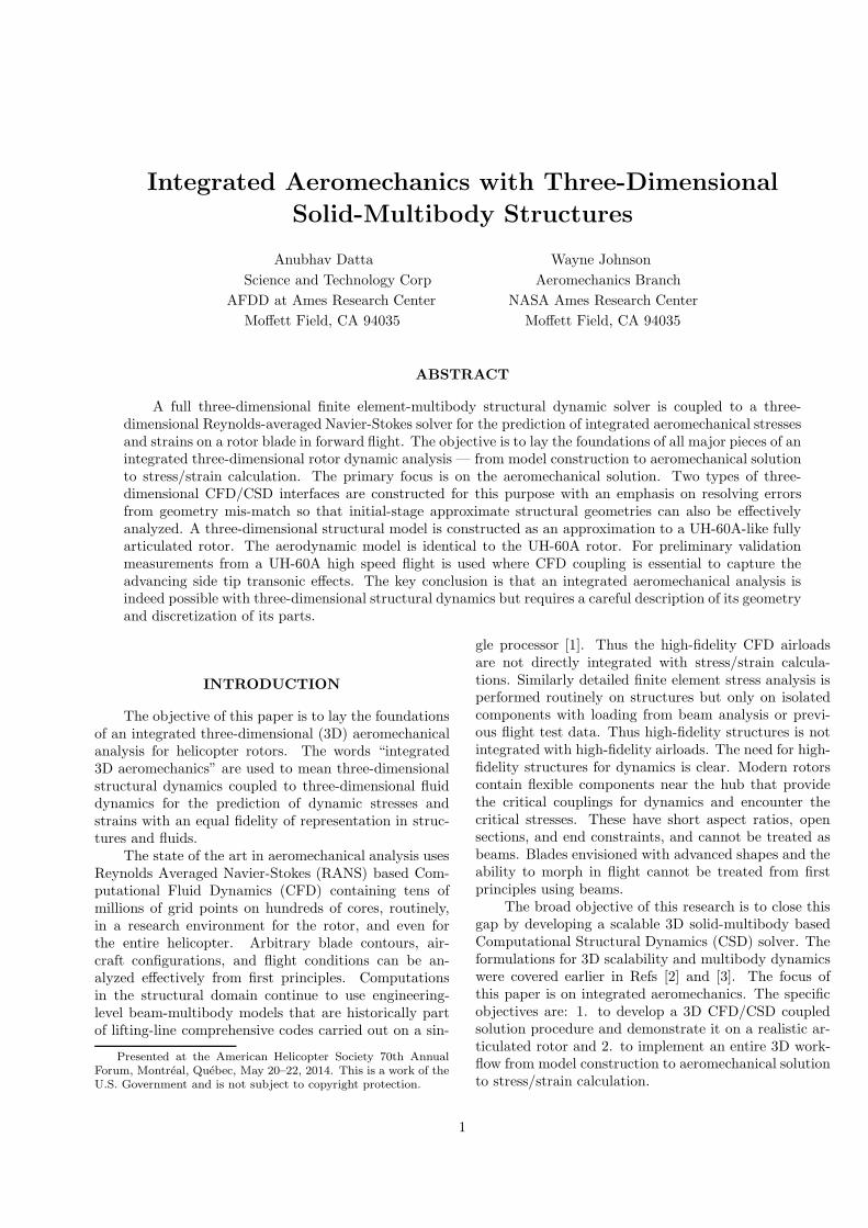
For the extraction of sectional properties, and forthe contruction of aerodynamic interfaces later, bladecross-sections must be defined. Figure 4 describes thedefinition (blade twist and some surface elements re-moved for illustration). Elements must supply nodes atthe leading and trailing edges and these nodes have tobe designated up-front as part of the model input. Theanalysis then defines the chord line and locates the 1/4−c(needed for CFD interface) and 3/4− c (needed for clas-sical aerodynamics) points. Two additional nodes, oneon the top surface and another at the bottom, are re-quired to define a nominal thickness line. It is used tosimply define the cross-sectional plane. It need not beperpendicular to the chord line thus any two points suf-fice as long as they are on the top and bottom surfaces.The key requirement is that all element faces line upalong the section. Thus even though the solver is natu-rally unstructured, sections can only be defined at spanstations where the elements line up. The geometry andgrid must be described accordingly for all span stationswhere sectional analysis is needed.

If ec is an unit vector aligned along the chord line

5

Thicknessline

Chordline

1/4−c

3/4−c

Trailing edge

Leading edge

Figure 4: Definition of cross-sectional planes.

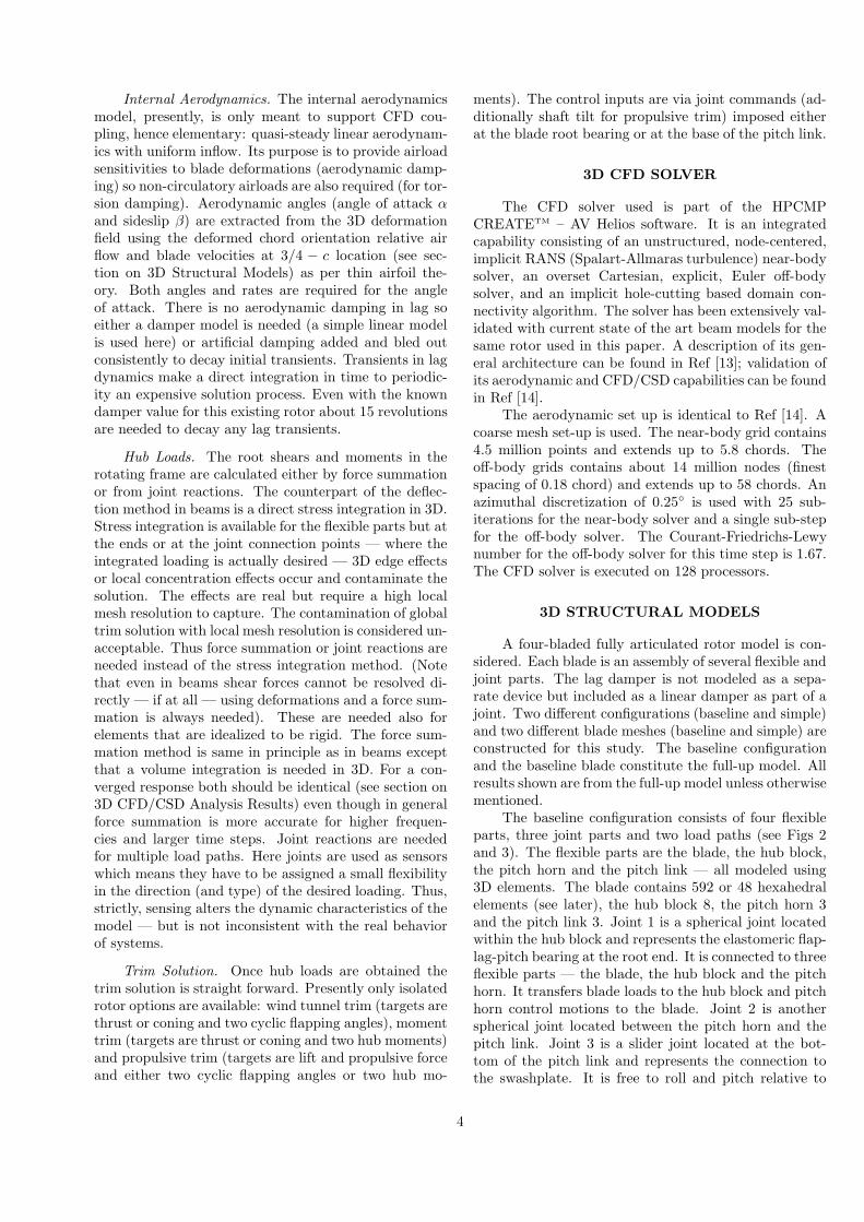
0 2 4 6 820,000

40,000

60,000

80,000

20,000

40,000

60,000

Span, m

GJ,

N−

m

Transverse loadingLateral loading

Figure 5: Calculation of torsional rigidity GJ.

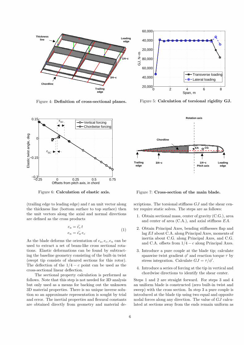
−0.25 0 0.25 0.5 0.75−0.3

−0.15

0

0.15

Offsets from pitch axis, in chord

Ela

stic

twis

t ang

le, d

eg

Vertical forcingChordwise forcing

zSC

ySC

Figure 6: Calculation of elastic axis.

Trailingedge

1/4−cPitch axis

Leadingedge

Rotation axis

3/4−c

Chordline

EA CG

Figure 7: Cross-section of the main blade.

(trailing edge to leading edge) and t an unit vector alongthe thickness line (bottom surface to top surface) thenthe unit vectors along the axial and normal directionsare defined as the cross products

ea = ec t

en = ea ec

(1)

As the blade deforms the orientation of ea, ec, en can beused to extract a set of beam-like cross sectional rota-tions. Elastic deformations can be found by subtract-ing the baseline geometry consisting of the built-in twist(swept tip consists of sheared sections for this rotor).The deflection of the 1/4 − c point can be used as thecross-sectional linear deflection.

The sectional property calculation is performed asfollows. Note that this step is not needed for 3D analysisbut only used as a means for backing out the unknown3D material properties. There is no unique inverse solu-tion so an approximate representation is sought by trialand error. The inertial properties and flexural constantsare obtained directly from geometry and material de-

scriptions. The torsional stiffness GJ and the shear cen-ter require static solves. The steps are as follows:

1. Obtain sectional mass, center of gravity (C.G.), areaand center of area (C.A.), and axial stiffness EA.

2. Obtain Principal Axes, bending stiffnesses flap andlag EI about C.A. along Principal Axes, moments ofinertia about C.G. along Principal Axes, and C.G.and C.A. offsets from 1/4− c along Principal Axes.

3. Introduce a pure couple at the blade tip; calculatespanwise twist gradient φ′ and reaction torque τ bystress integration. Calculate GJ = τ/φ′.

4. Introduce a series of forcing at the tip in vertical andchordwise directions to identify the shear center.

Steps 1 and 2 are straight forward. For steps 3 and 4an uniform blade is constructed (zero built-in twist andsweep) with the cross section. In step 3 a pure couple isintroduced at the blade tip using two equal and oppositenodal forces along any direction. The value of GJ calcu-lated at sections away from the ends remain uniform as

6

shown in Fig 5 and considered to be the cross-sectionalvalue. The calculations deviate near the root due to edgeeffects and the tip due to proximity to applied forcing asexpected. For the rectangular cross-section the classicalSt. Venant constant is recovered. The calculation of theshear center is show in Fig 6. Elastic twist from a setof vertical and chordwise forcing are interpolated to findthe zero cross over point and identify the location of theshear center. For no bending-twist coupling the shearcenter is a cross sectional property and remains uniformwith span.

The blade cross-section with the calculated offsetsare shown in Fig 7. Note that the blade is placed withpitch axis ahead of the rotation axis by the torque offset.The C.G. is placed close to and ahead of the pitch axisat 1/4−c. Then stability is guaranteed in the thin airfoilsense (aerodynamic center at 1/4−c). But the E.A. fallssignificantly behind the C.G. (by 13% c) which results ina strong flap-torsion coupling. The effect of this couplingis seen later in airloads. The C.G. location relative pitchaxis is similar to that of the UH-60A but its offset relativeE.A. is a substantial deviation.

3D CFD/CSD FORMULATION

The 3D CFD/CSD formulation includes the inter-face (spatial coupling) and solution procedure (temporalcoupling).

The interface deals with deformations sent to CFDand surface forcing sent to CSD. The deformations canbe described in one of two ways: as a 2D beam-like fieldor as a 3D field. The surface forcing can be describedin one of three ways: as 2D segmental airloads, as 3Dpatch forces, or as 3D surface pressures and shear. Itis assumed that the discretized surface will always dif-fer between CFD and CSD and hence corrections will berequired for conservation (same virtual work) and con-sistency (same integrated forcing). The difference is notmerely from mesh mis-match but unavoidable geometrymis-match — aerodynamic design will define the sur-face first while structural design will populate the sur-face last. Thus a method is desired that can be appliedeven when the internal structure is at an early designstage and does not necessarily carry on to the wettedsurface.

Deformation Interface

A 2D beam-like description of the deformation fieldallows the airfoil shapes in the fluid domain to be keptintact. While this description is the natural state of theart in beams, in 3D, they must be extracted from thedeflection field. The extraction is based on the deformedchord and thickness lines that describe the deformed ori-entation of the cross sectional plane. The cross sectionalplanes are defined as shown earlier in Fig 4. The extrac-tion excludes any cross-sectional flexibility — beyond

what is captured by the four nodes that define the lines— and appears to defeat the purpose of a 3D interfacebut is indeed the only means by which structures that areinternally incomplete can be analyzed. Thus integrated3D stress/strains can still be obtained at early stagesof structural design when only the main load-bearingpieces may be in place. The extraction procedure isstraight-forward: the direction cosines of the deformedcross-section: ea, en, ec, are used to extract three Eulerangles for any order of rotation. Standard limitationsnear ±π/2 apply but seldom encountered in rotor prob-lems. The order used here is lead-lag, flap, and pitch,consistent with mesh deformation.

A 3D description of the deformation field encountersthe problem of geometry and mesh mis-match. Ideally,there is a common 3D CAD geometry that populatesboth sides of the interface — CFD and CSD — so thata point in either domain can be associated with a cor-responding point on the other via geometry. A commongeometry description is beyond state of the art so theCFD mesh is presently considered to be the exact ge-ometry. The problem then reduces to associating eachCFD mesh point with its counterpart on the CSD sur-face. This parameterization is different in 3D and isthe basis for constructing an exact interface. Here ex-actness is defined as errors introduced due to interfacemis-match not exceeding those that are introduced bythe discretization of the individual solvers themselves.The parameterization is described under Level-II ForceInterface later.

Level-I Force Interface

The level-I force interface is an extension of thelower order aerodynamic interface with 2D airloads ad-mitted from CFD. Guaranteeing conservation is not pos-sible but consistency is achieved by the use of segmen-tal airloads (integrated over span-wise segments, seeRefs [14, 17] for methodology and validation). Theseairloads must now be distributed over the surface nodesof the segmental 3D elements. The nature of 2D air-loads implies the 3D finite element grid must ensure setsof surface elements along spanwise strips. Elements canbe unstructured within the strip but set boundaries mustline up along the chordwise direction. Then all surfacenodes within a segment are identified as aerodynamicinterface nodes.

In the present mesh the 3D elements are naturallyaligned in the spanwise direction therefore segments areeasy to define. Figure 8 shows two spanwise elementrows (blade twist and some surface elements removedfor illustration). Because the elements carry internalnodes there are five spanwise nodal lines. Assume thetwo ends represent the root and the tip. Then the aero-dynamic segments span half-way across either side ofeach nodal line. So there are as many segments as thereare nodal lines. Each segment receives dimensional air-

7

SEG 3SEG 4

SEG 5

SEG 2SEG 1

Surfacenodes

Figure 8: Level-I force interface.

loads from CFD with pitching moment about the 1/4−c.These are then distributed over the segmental nodes inan assumed manner — linearly for lift (along chord, in-creasing toward leading edge) and quadratically for drag(along thickness) — as functions of three constants to besolved at each azimuth and radial station from the CFDairloads. If y and z are the chordwise (toward leadingedge) and thickness wise (to upper surface) coordinatesand FZ , FY and M are the vertical, in-plane and 1/4− cpitching moments then the nodal forces fZ and fY inthe vertical and in-plane directions are represented as

fZ = α0 + α1(y − y25)

fY = β0 + α1(z − z25)2

(2)

with the three constants α0, α1 and β0 solved using thethree airloads

FZ =∑

fZ

FY =∑

fY

M25 =∑

[fZ(y − y25) − fY (z − z25)]

(3)

The subscript 25 denotes 1/4 − c quantities. The sum-mation is over all n segmental nodes. The axial forceFX , although negligible compared to the inertial force,is simply distributed at each node as fX = FX/n.

The internal stresses from the level-I interface areonly as good as the assumed representation and there-fore ad hoc. It is a convenient interface for initial veri-fication because it leaves the Delta Coupling procedureintact. This interface is used later for a fully coupledsolution. But a 3D CSD model opens opportunity for adetailed interface with which exact internal stresses canbe calculated. This is described below.

Level-II Force Interface

The level-II force interface is an exact 3D patch forceinterface. Consistency is guaranteed but conservationachieved only at the limit of fluid and structural mesh

refinements. In this interface each CFD surface meshpoint (or the center of each surface triad or quad —depending on how the surface stresses are integrated inthe fluid domain to generate a patch force) is first asso-ciated uniquely with a CSD surface coordinate. Ideally,as noted earlier, a point on the exact geometry should beassociated not a point on the CFD mesh, but in absenceof a geometry module that populates both sides of theinterface, the CFD mesh is assumed to be the exact ge-ometry. The method is generic to mis-matched meshes.Given a CFD surface point — regardless of whether itlies on the CSD surface or not — an unique set of CSDsurface parameters are calculated. This parameteriza-tion is based only on the natural coordinates and shapefunctions of the elements.

Within an element (including its surface) the geo-metric coordinates are related to the curvilinear naturalcoordinates as

x = x(ξ, η, ζ)

y = y(ξ, η, ζ)

z = z(ξ, η, ζ)

(4)

where −1 ≤ ξ, η, ζ ≤ 1. Because the relationship is non-linear, given a target point (x , y , z)T , its correspondingnatural coordinates (ξ η ζ) must be found iteratively.The iterations can be started from any of the elementnodes — where both (ξ η ζ)0 and (x y z)0 are known —and continued as per Newton-Raphson to convergence.

k = 0, 1, 2, . . .xξ xη xζ

yξ yη yζ

zξ zη zζ

∆ξ∆η∆ζ

k

=

xyz

T

−

xyz

k

(5)

The left hand side gradient matrix (where xζ = ∂x/∂ξand so on) is the transpose of the Jacobian of the co-ordinate transformation. As long as the target pointlies within or on the element and the element is well-behaved (i.e. has a well-conditioned Jacobian) the iter-ations will converge to an unique solution. Thus if theCFD point is on the surface (matched interface) its nat-ural coordinates can be readily obtained using this basicprocedure. A generic procedure is one that will obtaina corresponding set of natural coordinates for all pointsincluding those that are out of surface but collapse tothe basic procedure for points on surface. Two differentgeneric procedures are proposed as follows.

Method 1: Gradient extrapolation. Let ζ = 1 be thesurface (see Fig 9). An out of surface point is associ-ated with a surface point (ξ, η) if the surface coordinateζ leaves the surface in such a direction that it passesthrough the point. Thus the method can be termed agradient extrapolation method as the gradient of the sur-face coordinate (ζ) is extrapolated. Note that all out ofsurface points that lie along the direction of extrapo-lation will be associated with the same — but unique

8

— CSD point. To identify this point the same itera-tions as Eq 5 are used but the gradient matrix is alwaysevaluated at the surface (ζ = 1 in this example). Theiterations will drive the absolute value of ζ to greaterthan 1, confirming the point lies outside the surface, butwill converge in ξ and η. If not, or if the absolute valuesof either of these converged coordinates are greater than1, then the point is rejected by the ζ = 1 surface. Allsurfaces defined as fluid interfaces are checked one byone and if the point is rejected by all it is rejected by theelement. If rejected by all elements it is eliminated fromthe interface and tagged instead as a candidate for er-ror calculation. Figure 9 shows an example of successfulextraction of surface parameters using this method.

Method 2: Orthogonal projection. Let ζ = 1 be thesurface (see Fig 9). An out of surface point is associatedwith the nearest surface coordinate (ξ, η) (note that thisis not the nearest neighbor method where the associationis to the nearest node). This means the normal to thesurface at that coordinate passes through the point. Thesurface coordinates are obtained by

k = 0, 1, 2, . . .xξ xη

yξ yη

zξ zη

(∆ξ∆η

)

k

=

xyz

T

−

xyz

k

(6)

A Moore-Penrose inverse of the left hand side matrix(A+ = (ATA)−1AT ) solves the above equation in theleast square sense and finds the nearest surface coordi-nate. If the absolute values of either of the convergedcoordinates are greater than 1 then the point does notbelong to the ζ = 1 surface. As in method 1 all surfacesof all elements are checked one by one for inclusion orelimination from the interface. Figure 9 shows an exam-ple of successful extraction of surface parameters usingthis method. Figure 10 shows an example of rejectionwhere the extracted surface parameters lie outside theelement.

The surface coordinates produced by the two meth-ods are different (Fig. 9). In general the farther the pointfrom the surface the greater the difference. Only whenthe element boundaries are orthogonal the two methodsconverge. Because then the coordinate leaving the sur-face (used in method 1) is the surface normal (used inmethod 2). In general either method can be used withthe difference compensated for by the interface error cal-culation (see below). For each CFD surface node thecorresponding CSD element and its natural coordinatesξ, η, ζ then complete the surface parameterization. Thedisplacement of each CFD node and the virtual workcontribution of the patch force occurring at that nodeare now precisely defined.

Force interface error. Even though the interface isexact — the errors now stem entirely from geometry de-scription of the individual solvers and not how variables

CFDsurface

point

Startingpoint

η

ξ

Iterative search forCSD surface point

(method 2)

Iterative search forCSD surface point

(method 1)

CSDsurfaceelement

Figure 9: An example of an out of surface CFDpoint for which CSD surface parameters couldbe extracted successfully.

Iterative search forCSD surface point

CSDsurfaceelement

CFDsurface

point

ξ

η

Figure 10: An example of an out of surfaceCFD point for which CSD surface parameterscould not be extracted successfully.

are exchanged between them — it can lead to significanterrors or can even break down (large number of pointseliminated from interface) when the underlying struc-tural model is incomplete. It is important that theseerrors be accounted for so that meaningful stress calcula-tions are still possible at early stages of structural design.For this purpose the error is defined in terms of segmen-tal airloads. For all CFD nodes that are eliminated fromthe interface (i.e., not claimed by any CSD element) theerror is simply its contribution to the segmental airload.For all others, the error is only in form of a segmentalpitching moment, calculated based on the distance be-tween the CFD coordinate and its corresponding CSDcoordinate. The segmental airloads (errors) are then re-introduced into the structure through a level-I interface.For no mis-match the error vanishes. For a 100% mis-match level-II collapses to level-I — since every point isthen rejected and re-introduced through level-I.

9

Green: 1−5000 pts

Cyan: 15,001−20,000 pts

Red: 5001−10,000 pts

Blue: 20,000−24,761 pts

Magenta: 10,001−15,000 pts

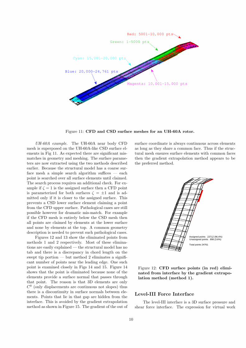
Figure 11: CFD and CSD surface meshes for an UH-60A rotor.

UH-60A example. The UH-60A near body CFDmesh is superposed on the UH-60A-like CSD surface el-ements in Fig 11. As expected there are significant mis-matches in geometry and meshing. The surface parame-ters are now extracted using the two methods describedearlier. Because the structural model has a coarse sur-face mesh a simple search algorithm suffices — eachpoint is searched over all surface elements until claimed.The search process requires an additional check. For ex-ample if ζ = 1 is the assigned surface then a CFD pointis parameterized for both surfaces ζ = ±1 and is ad-mitted only if it is closer to the assigned surface. Thisprevents a CSD lower surface element claiming a pointfrom the CFD upper surface. Pathological cases are stillpossible however for dramatic mis-match. For exampleif the CFD mesh is entirely below the CSD mesh thenall points are claimed by elements at the lower surfaceand none by elements at the top. A common geometrydescription is needed to prevent such pathological cases.

Figures 12 and 13 show the eliminated points frommethods 1 and 2 respectively. Most of these elimina-tions are easily explained — the structural model has notab and there is a discrepancy in chord length on theswept tip portion — but method 2 eliminates a signifi-cant number of points near the leading edge. One suchpoint is examined closely in Figs 14 and 15. Figure 14shows that the point is eliminated because none of theelements provide a surface normal that passes throughthat point. The reason is that 3D elements are onlyC0 (only displacements are continuous not slopes) thusthere is a discontinuity in surface normals between ele-ments. Points that lie in that gap are hidden from theinterface. This is avoided by the gradient extrapolationmethod as shown in Figure 15. The gradient of the out of

surface coordinate is always continuous across elementsas long as they share a common face. Thus if the struc-tural mesh ensures surface elements with common facesthen the gradient extrapolation method appears to bethe preferred method.

Assigned points 23712 (96.4%)Unassigned points 898 (3.6%)

Total points 24761

Figure 12: CFD surface points (in red) elimi-nated from interface by the gradient extrapo-lation method (method 1).

Level-III Force Interface

The level-III interface is a 3D surface pressure andshear force interface. The expression for virtual work

10

Assigned points 23712 (95.8%)Unassigned points 1049 (4.2%)

Total points 24761

Figure 13: CFD surface points (in red) elimi-nated from interface by the orthogonal pro-jection method (method 2).

Element 1

Element 2

CFD point

η

η

Figure 14: A leading edge CFD surfacepoint eliminated by the orthogonal projectionmethod.

integrates terms involving both fluid stresses and struc-tural surface normals. Because conservation requiresall interpolation to be carried out using correspondingshape functions in each domain [16], either fluid stressesmust be supplied at all structural Gauss points (if in-tegrating in the CSD domain) or structural shape func-tions supplied at fluid mesh points (if integrating in theCFD domain). Then conservation is guaranteed but con-sistency is still achieved only at the limit of fluid andstructural mesh refinement. For different mesh resolu-tions the integrated forces will remain different in CFDand CSD domains. This is undesirable for rotor prob-lems where accuracy of the trim state is essential. Thusthe level-II interface is considered the most desired. Thelevel-I interface is an approximation of level-II and isused for integrated analysis as the first step.

Element 1

Element 2

CFD point

Figure 15: A leading edge CFD surfacepoint admitted by the gradient extrapolationmethod.

CFD/CSD solution procedure

The level-I force interface is used. Thus the con-ventional Delta Coupling procedure of Johnson (LooseCoupling in rotorcraft terminology) can be retained withsegmental airloads (dimensional) used as the delta vari-ables. (Ref [18] is the original invention, the current im-plementation follows Ref [19]). The level-II force inter-face requires an advanced formulation with the surfaceelement generalized loading used as the delta variables.This method was proposed and validated in Ref [17] forbeams but not yet implemented in the current solver.The 2D deformation interface is used. Thus the conven-tional beam-like mesh deformation procedures can beretained in the CFD solver. The 3D deformation inter-face requires a mesh deformation method that is beyondscope of the current solver. Thus an integrated solutionis obtained using the simplest of the interfaces.

As per the Delta Coupling procedure periodic air-loads and deformations are exchanged. This accommo-dates unequal time steps in the fluid and structural do-mains naturally — 0.25◦ and 3◦ respectively — withairloads and deformations digitally filtered (Fourier in-terpolation, 12 harmonics used here) during exchange.Although airloads are available at the CSD time steps,deformations are not available at the CFD time steps,hence an interpolation is always needed. But because theCSD solution is obtained by time integration this inter-polation cannot be made consistent with the solver whileat the same time provide smooth grid motion across CFDtime steps. Thus time accuracy cannot be ensured —not even at 3◦ intervals. The alternative — to marchCFD and CSD together with intermittent sub-iterations— though straight forward is practically unacceptable inrotorcraft as the structural dynamics takes 30−40 revo-lutions to attain the trimmed periodic solution whereas

11

0 90 180 270 360−1

−0.5

0

0.5

1x 10

5

Azimuth, deg

lb−

ft

AeroInertialTotal

Figure 16: Flap moment at root bearing.

0 90 180 270 360−2

−1

0

1

2x 10

4

Azimuth, deg

lb−

ft

AeroInertialTotal

Figure 17: Lead-lag moment at root bearing.

0 90 180 270 360−4000

−3000

−2000

−1000

0

1000

Azimuth, deg

lb−

ft

AeroInertialTotal

Figure 18: Pitch moment at root bearing.

0 90 180 270 360

−3000

−2000

−1000

0

1000

2000

Azimuth, deg

lb−

ft

Force summationJoint reaction

Lead−lag

Flap

Pitch

Figure 19: Joint reactions at root bearing.

the fluid solution settles rapidly to periodicity within1 − 2 revolutions. And because the fluid solution set-tles rapidly, advancing the solver by only a quarter ofa revolution can allow nominally periodic airloads to beconstructed using all four blades. The coupling processuses half a revolution for the first two CFD iterationsand quarter revolutions there after.

As per the Delta Coupling procedure the simpleinternal aerodynamic model is retained in CSD as apreconditioner for convergence. An isolated rotor trimmodel is used with thrust and two hub moments targetedusing collective and cyclic commands imposed as pitchlink displacements. The trim Jacobian is calculated onceusing the internal aerodynamic model and requires noupdate for all coupling iterations for the flight conditionstudied.

3D CFD/CSD ANALYSIS RESULTS

The UH-60A flight test counter 8534 (advance ra-tio µ = 0.368, nondimensional thrust CT /σ = 0.084 andshaft tilt αS = −7.31◦ (forward)) is considered. It isa high speed (158 kts) high vibration level flight where

the dominant airloads are the 3D unsteady tip transonicpitching moments and hence CFD is essential. Eventhough the blade structural properties are not identicalto UH-60A the aerodynamic characteristics (geometryand grid) are the same and therefore comparing predic-tions with UH-60A test data provides a reasonable basisfor qualitative validation.

Dynamic Response

The time step required for stability and convergenceof the dynamic response is observed to be governed bythe nonlinearities introduced by the joint not the sizeof the finite element mesh. Thus the simple blade andthe baseline blade both require the same time step forthe same hub configuration. It is also observed that thedominant source of nonlinearity is the elastomeric bear-ing where the trim commands are imposed. Hence thesimple hub and the baseline hub also have the same timestep requirement — as the bearing is common to both.The strong nonlinearities require the calculation of dy-namic stiffness at every time step. Calculating it onceabout a trim solution or updating it every few time steps

12

diverges the solution quickly. Under these considera-tions both time integration methods (the Generalized-αwas executed at its simplest Newmark form) convergesto the same results. Sub-iterations are possible at ev-ery time step but needed only for relatively large steps.Typically 3− 5 sub-iterations were required to drive theresidual down to 10−5 at each time step. Sub-iterationsare also required for the consistency of inertial loads withthe response solution. For the purposes of CFD couplingsmaller time steps were preferred over larger steps withsub-iterations so as to minimize errors from deformationinterpolation. Thus instead of ∆ψ = 9◦ with 3 − 4 sub-iterations, ∆ψ = 3◦ with no sub-iterations was preferred.The results shown are all obtained using ∆ψ = 3◦ withno sub-iterations.

The blade dynamic response is verified by studyingthe inertial loads and joint reactions. Simple aerody-namics (without CFD) is adequate for this purpose. Toverify root reactions the simpler configuration is usedwhere the pitch link stiffness is lumped at the bearingand the control angles are imposed as command sig-nals at the bearing. Figures 16, 17 and 18 show theintegrated aerodynamic, inertial and total (aerodynamicplus inertial) moments at the elastomeric bearing for flap(positive down), lead-lag (positive forward) and pitch(nose up) motions. The equal and opposite nature ofthe aerodynamic and inertial flap moments verifies thefundamental dynamics of the blade. It is not identi-cally zero because of a small amount of stiffness anddamping at the bearing. The damping is significantlylarger in lag (due to the lag damper) which is reflectedin the more substantial lead lag moment. The stiffnessis significantly larger in pitch (due to pitch link stiffness)so that the root reaction follows the aerodynamic forc-ing closely. The inertial loading calculation, and hencethe velocity and acceleration calculations, are verified bycomparing these integrated moments obtained by forcesummation with reaction forces obtained directly fromjoint response at the bearing. This comparison is af-fected by the solver time step as mentioned earlier butagrees closely for ∆ψ = 3◦ as shown in Fig 19. The jointreactions are left in the joint frame to illustrate the effectof order of rotations. The force summation results arealong the undeformed blade frame. Because the order ofjoint rotation is lead-lag first then flap and then torsiononly the lead-lag comparison is exact, the flap and tor-sion moments have to be transferred to the undeformedframe for exact verification. Henceforth all results shownuse the force summation method.

CFD/CSD Airloads

The convergence of the CFD/CSD analysis proceedsas shown by the mean normal force distribution fromCFD in Fig 20. Iteration-0 shows CFD airloads calcu-lated using deformations from the baseline trim solu-tion (with internal aerodynamics). By Iteration-7 the

airloads and dynamic response have nearly converged.Henceforth all airloads are shown from both the last twoiterations 6 and 7. It is known that the flight test normalforce shows a greater thrust at this condition than whatcan be achieved by the trim target.

0 0.2 0.4 0.6 0.8 10

100

200

300

400

r/R

lb/ft

Iter 0Iter 1Iter 2Iter 3Iter 4Iter 5Iter 6Iter 7

Flight

Analysis

Figure 20: Steady normal force convergence from3D CFD/CSD using level-1 interface; predictionscompared with measured UH-60A airloads forqualitative comparison.

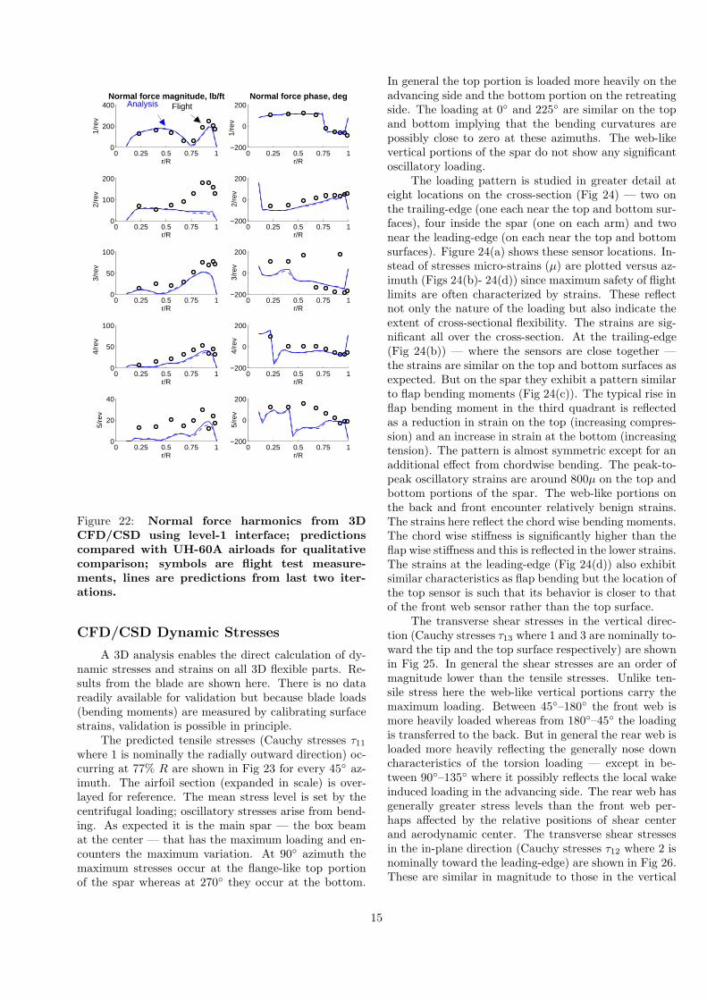
The detailed sectional airloads at three span wisestations are shown in Fig 21. Clearly the normal forcesdeviate significantly from the UH-60A values particu-larly at the outboard stations (inboard of 67.5%R predic-tions are good and hence not shown). The discrepancy ispartly because of the less severe transonic pitching mo-ment drop at the first quadrant close to the tip (96.5%R)due to a different blade dynamics than the UH-60A butmainly for reasons revealed in Fig 22. Figure 22 showsthe harmonics of the normal force across the blade span.Forcing that are passed to CSD is plotted (divided bysegment lengths) so the spanwise resolution is the sameas the number of aerodynamic segments in the model (33segments). The 1/rev phase with its distinct 180◦ shiftover the span verifies the accuracy of the trim solution.All the vibratory harmonics (3−5/rev) are well predictedwith at least the same accuracy achieved by current UH-60A beam models coupled to CFD. The main discrep-ancy is from the 2/rev airloads. These are determined bya large 1/rev torsion at this high speed condition. The1/rev torsion in the current analysis deviate significantlyfrom the UH-60A due to the very high (13% c) C.G. off-set from the E.A. (Fig 7). The 1/rev torsion magnitudeis as expected (about negative 4◦ peak to peak) but thephase is contaminated by 1/rev flap. Thus a proper val-idation of a 3D analysis requires a more careful assign-ment of material properties so that at least the majoroffsets (E.A. and C.G.) are precisely placed.

13

0 90 180 270 360−40

−20

0

20

401/4−c pitching moment

lb−

ft/ft

0 90 180 270 360−400

−200

0

200

400Normal Force

lb/ft

0 90 180 270 360−50

0

50Chord Force

lb/ft

0 90 180 270 360−80

−60

−40

−20

0

20

40

lb−

ft/ft

0 90 180 270 360−600

−400

−200

0

200

400

lb/ft

0 90 180 270 360−50

0

50

lb/ft

0 90 180 270 360−120

−100

−80

−60

−40

−20

0

20

40

Azimuth, deg

lb−

ft/ft

0 90 180 270 360−600

−400

−200

0

200

400

Azimuth, deg

lb/ft

0 90 180 270 360−50

0

50

Azimuth, deg

lb/ft

67.5% R67.5% R67.5% R

86.5% R 86.5% R86.5%R

96.5% R 96.5% R 96.5% R

Flight

Analysis

Figure 21: Airloads from 3D CFD/CSD using level-1 interface; predictions from last two iterationscompared with measured UH-60A airloads for qualitative comparison.

14

0 0.25 0.5 0.75 10

200

400

r/R

1/re

vNormal force magnitude, lb/ft

0 0.25 0.5 0.75 1−200

0

200

r/R

1/re

v

Normal force phase, deg

0 0.25 0.5 0.75 10

100

200

r/R

2/re

v

0 0.25 0.5 0.75 1−200

0

200

r/R2/

rev

0 0.25 0.5 0.75 10

50

100

r/R

3/re

v

0 0.25 0.5 0.75 1−200

0

200

r/R

3/re

v

0 0.25 0.5 0.75 10

50

100

r/R

4/re

v

0 0.25 0.5 0.75 1−200

0

200

r/R

4/re

v

0 0.25 0.5 0.75 10

20

40

r/R

5/re

v

0 0.25 0.5 0.75 1−200

0

200

r/R

5/re

v

Analysis Flight

Figure 22: Normal force harmonics from 3DCFD/CSD using level-1 interface; predictionscompared with UH-60A airloads for qualitativecomparison; symbols are flight test measure-ments, lines are predictions from last two iter-ations.

CFD/CSD Dynamic Stresses

A 3D analysis enables the direct calculation of dy-namic stresses and strains on all 3D flexible parts. Re-sults from the blade are shown here. There is no datareadily available for validation but because blade loads(bending moments) are measured by calibrating surfacestrains, validation is possible in principle.

The predicted tensile stresses (Cauchy stresses τ11where 1 is nominally the radially outward direction) oc-curring at 77% R are shown in Fig 23 for every 45◦ az-imuth. The airfoil section (expanded in scale) is over-layed for reference. The mean stress level is set by thecentrifugal loading; oscillatory stresses arise from bend-ing. As expected it is the main spar — the box beamat the center — that has the maximum loading and en-counters the maximum variation. At 90◦ azimuth themaximum stresses occur at the flange-like top portionof the spar whereas at 270◦ they occur at the bottom.

In general the top portion is loaded more heavily on theadvancing side and the bottom portion on the retreatingside. The loading at 0◦ and 225◦ are similar on the topand bottom implying that the bending curvatures arepossibly close to zero at these azimuths. The web-likevertical portions of the spar do not show any significantoscillatory loading.

The loading pattern is studied in greater detail ateight locations on the cross-section (Fig 24) — two onthe trailing-edge (one each near the top and bottom sur-faces), four inside the spar (one on each arm) and twonear the leading-edge (on each near the top and bottomsurfaces). Figure 24(a) shows these sensor locations. In-stead of stresses micro-strains (µ) are plotted versus az-imuth (Figs 24(b)- 24(d)) since maximum safety of flightlimits are often characterized by strains. These reflectnot only the nature of the loading but also indicate theextent of cross-sectional flexibility. The strains are sig-nificant all over the cross-section. At the trailing-edge(Fig 24(b)) — where the sensors are close together —the strains are similar on the top and bottom surfaces asexpected. But on the spar they exhibit a pattern similarto flap bending moments (Fig 24(c)). The typical rise inflap bending moment in the third quadrant is reflectedas a reduction in strain on the top (increasing compres-sion) and an increase in strain at the bottom (increasingtension). The pattern is almost symmetric except for anadditional effect from chordwise bending. The peak-to-peak oscillatory strains are around 800µ on the top andbottom portions of the spar. The web-like portions onthe back and front encounter relatively benign strains.The strains here reflect the chord wise bending moments.The chord wise stiffness is significantly higher than theflap wise stiffness and this is reflected in the lower strains.The strains at the leading-edge (Fig 24(d)) also exhibitsimilar characteristics as flap bending but the location ofthe top sensor is such that its behavior is closer to thatof the front web sensor rather than the top surface.

The transverse shear stresses in the vertical direc-tion (Cauchy stresses τ13 where 1 and 3 are nominally to-ward the tip and the top surface respectively) are shownin Fig 25. In general the shear stresses are an order ofmagnitude lower than the tensile stresses. Unlike ten-sile stress here the web-like vertical portions carry themaximum loading. Between 45◦–180◦ the front web ismore heavily loaded whereas from 180◦–45◦ the loadingis transferred to the back. But in general the rear web isloaded more heavily reflecting the generally nose downcharacteristics of the torsion loading — except in be-tween 90◦–135◦ where it possibly reflects the local wakeinduced loading in the advancing side. The rear web hasgenerally greater stress levels than the front web per-haps affected by the relative positions of shear centerand aerodynamic center. The transverse shear stressesin the in-plane direction (Cauchy stresses τ12 where 2 isnominally toward the leading-edge) are shown in Fig 26.These are similar in magnitude to those in the vertical

15

2 4 6 8 10 12 14 16 18

x 107

−1012

(a) Azimuth ψ = 0◦

2 4 6 8 10 12 14 16 18

x 107

−1012

(b) Azimuth ψ = 45◦

2 4 6 8 10 12 14 16 18

x 107

−1012

(c) Azimuth ψ = 90◦

2 4 6 8 10 12 14 16 18

x 107

−1012

(d) Azimuth ψ = 135◦

2 4 6 8 10 12 14 16 18

x 107

−1012

(e) Azimuth ψ = 180◦

2 4 6 8 10 12 14 16 18

x 107

−1012

(f) Azimuth ψ = 225◦

2 4 6 8 10 12 14 16 18

x 107

−1012

(g) Azimuth ψ = 270◦

2 4 6 8 10 12 14 16 18

x 107

−1012

(h) Azimuth ψ = 315◦

Figure 23: Dynamic tensile stresses (τ11) predicted using 3D CFD/CSD analysis; 77% R station;colormap range: 106 − 18 × 107 N/m2 (Pascal).

16

Trailingedge

sensorsSpar

sensors

Leadingedge

sensors

(a) Strain sensor locations; two at the trailing-edge, four on the mainspar and two near the leading-edge.

0 90 180 270 360400

800

1200

1600

Azimuth, deg

Mic

rost

rain

, µ

BottomTop

(b) Strains at the trailing-edge.

0 90 180 270 360400

800

1200

1600

Azimuth, deg

Mic

rost

rain

, µ

Back WBottom FTop FFront W

(c) Strains at the spar

0 50 100 150 200 250 300 350400

600

800

1000

1200

1400

1600

Azimuth, deg

Mic

rost

rain

, µ

BottomTop

(d) Strains at the leading-edge

Figure 24: Azimuthal variation of tensile strains (ǫ11) predicted using 3D CFD/CSD analysis; 77% Rstation.

direction but they occur at different locations. Like thetensile stresses, here the flange-like portions of the sparexhibit the maximum loading. But in terms of grossloading they exhibit the same general pattern as thevertical shears — the rear web is loaded more heavilyreflecting the generally nose down characteristics of thetorsion loading except in between 90◦–135◦ azimuths.

The generic nature of the blade and the approximatenature of the level-I interface make specific conclusionson the details of stress/strain variations premature forthis rotor but the results above appear consistent withtypical patterns of loading and reveal the type of detailedstress/strain analysis possible using 3D structures.

CONCLUSIONS

A full three-dimensional finite element-multibodystructural dynamics solver was coupled to a three-dimensional Reynolds-averaged Navier-Stokes solver forthe prediction of integrated stresses and strains on a ro-tor blade in forward flight. All major pieces of the 3Dworkflow were implemented and analyzed. The struc-

tural model was an idealized representation of a fullyarticulated UH-60A-like rotor. The aerodynamic modelwas identical to the UH-60A rotor. The primary focusof this work was on the 3D CFD/CSD coupled solutionprocedure. Two different types of 3D interfaces were de-veloped and the simpler of the two implemented. Thecoupled airloads were compared with flight test data.The coupled 3D blade stresses and strains were stud-ied for generic patterns typical of rotors in high speedforward flight. Based on this work the following keyconclusions are drawn.

1. An integrated aeromechanical analysis with a high-fidelity 3D representation of the structure can in-deed be carried out for helicopter rotors in forwardflight. Dynamic stresses and strains resulting fromaerodynamic loading can then be calculated with-out any reduced order approximation. Advancedhub types and blade shapes can then be modeledwithout any reduced order assumption.

2. The convergence of the (implicit) CSD solver re-quires dynamic stiffness to be updated at every time

17

−5 0 5 10 15 20

x 106

−1012

(a) Azimuth ψ = 0◦

−5 0 5 10 15 20

x 106

−1012

(b) Azimuth ψ = 45◦

−5 0 5 10 15 20

x 106

−1012

(c) Azimuth ψ = 90◦

−5 0 5 10 15 20

x 106

−1012

(d) Azimuth ψ = 135◦

−5 0 5 10 15 20

x 106

−1012

(e) Azimuth ψ = 180◦

−5 0 5 10 15 20

x 106

−1012

(f) Azimuth ψ = 225◦

−5 0 5 10 15 20

x 106

−1012

(g) Azimuth ψ = 270◦

−5 0 5 10 15 20

x 106

−1012

(h) Azimuth ψ = 315◦

Figure 25: Dynamic shear stresses in vertical direction (τ13) predicted by 3D CFD/CSD analysis; 77%R station; colormap range: −5 × 106 − 20 × 106 N/m2 (Pascal).

18

−5 0 5 10 15 20

x 106

−1012

(a) Azimuth ψ = 0◦

−5 0 5 10 15 20

x 106

−1012

(b) Azimuth ψ = 45◦

−5 0 5 10 15 20

x 106

−1012

(c) Azimuth ψ = 90◦

−5 0 5 10 15 20

x 106

−1012

(d) Azimuth ψ = 135◦

−5 0 5 10 15 20

x 106

(e) Azimuth ψ = 180◦

−5 0 5 10 15 20

x 106

−1012

(f) Azimuth ψ = 225◦

−5 0 5 10 15 20

x 106

−1012

(g) Azimuth ψ = 270◦

−5 0 5 10 15 20

x 106

−1012

(h) Azimuth ψ = 315◦

Figure 26: Dynamic shear stresses in in-plane direction (τ12) predicted by 3D CFD/CSD analysis; 77%R station; colormap range: −5 × 106 − 20 × 106 N/m2 (Pascal).

19

step. This is due to the strong non-linearities intro-duced by joints unified within 3D elements. For rel-atively large time steps sub-iterations are required— both for the accuracy of the response solutionas well as for consistency of inertial loads with theresponse solution.

3. The time step is not dictated by the mesh resolu-tion of the flexible 3D parts but rather by the non-linearities introduced by the joints. Thus a fine-mesh problem could be solved with the same stabil-ity and convergence behavior using the same timestep as long as the trim conditions (joint motions)remained similar.

4. It is not essential that the finite element internalstructure be populated in every detail for a nominalapplication of the analysis. The 3D interface canbe made generic enough to accommodate an incom-plete internal structure provided the primary loadbearing pieces are in place. But a careful descrip-tion of the material properties of these pieces arerequired so that the major blade offsets (E.A. andC.G.) are correctly located.

In the end we note that even though the CSD solveris parallel and scalable it was executed on a single pro-cessor in this study. The structural geometry, mesh,and material descriptions were representative of a re-alistic rotor but inexact and coarse. The exact patchforce based level-II interface was developed but only theapproximate level-I interface was implemented for inte-grated solution. A time integration procedure is an inef-ficient solution process to reach a periodic trim solutionin a low-damped near resonance system like rotorcraft.These and other topics remain the subjects of futurework.

REFERENCES

[1] Johnson, W., “A History of Rotorcraft Compre-hensive Analyses,” NASA/TP-2012-216012.

[2] Datta, A. and Johnson, W., “Three-dimensionalFinite Element Formulation and Scalable DomainDecomposition for High Fidelity Rotor DynamicAnalysis,” Journal of the American Helicopter So-

ciety, Vol. 56, (2), July 2011, pp. 1–14.

[3] Datta, A. and Johnson, W., “A Multibody For-mulation For Three Dimensional Brick Finite Ele-ment Based Parallel and Scalable Rotor DynamicAnalysis,” American Helicopter Society 66th An-nual Forum Proceedings, Phoenix, AZ, May 11–13,2010.

[4] Smith, M. J., Hodges, D. H., and Cesnik, C. E.S., “Evaluation of Computational Algorithms Suit-able for Fluid-Structure Interactions,” Journal of

Aircraft, Vol. 37, (2), March–April 2000, pp. 282–294.

[5] Dowell, E. H. and Hall, K. C., “Modeling of Fluid-Structure Interaction,” Annual Review of Fluid

Mechanics, Vol. 33, pp. 445–490, January 2001.

[6] Datta, A and Johnson, W., “An Assessment of theState-of-the-art in Multidisciplinary Aeromechan-ical Analyses,” American Helicopter Society Spe-cialists’ Conference on Aeromechanics, San Fran-cisco, CA, January 23–25, 2008.

[7] Hou, G., Wang, J. and Layton, A., “Numer-ical Methods for Fluid-Structure Interaction —A Review,” Communications in Computational

Physics, Vol. 12, (2), August 2012, pp. 337–337.

[8] Bazilevs, Y., Takizawa, K. and Tezduyar, T. E.,Computational Fluid-Structure Interaction: Meth-

ods and Applications, John Wiley & Sons Ltd, UK,2013.

[9] Staruk, W., Chopra, I. and Datta, A., “Three-Dimensional CAD-Based Structural Modeling forNext Generation Rotor Dynamic Analysis,” Amer-ican Helicopter Society 70th Annual Forum Pro-ceedings, Montreal, Quebec, May 20–22, 2014.

[10] Blackford, L. S., Choi, J., Cleary, A., D’Azevedo,E., Demmel, J., Dhillon, I., Dongarra, J., Ham-marling, S., Henry, G., Petitet, A., Stanley, K.,Walker, D. and Whaley, R. C., ScaLAPACK

Users’ Guide, Society for Industrial and AppliedMathematics, Philadelphia, PA, 1997.

[11] Kuhl, D. and Crisfield, M. A., “Energy-conservingand Decaying Algorithms in Non-linear StructuralDynamics,” International Journal for Numerical

Methods in Engineering, Vol. 45, (5), June 1999,pp. 569–599.

[12] Bathe, K., “Conserving Energy and Momentumin Nonlinear Dynamics: A Simple Implicit TimeIntegration Scheme,” Computers and Structures,Vol. 85, (7-8), April 2007, pp. 437–445.

[13] Strawn, R., “High-Performance Computing forRotorcraft Modeling and Simulation,” Computing

in Science and Engineering, Vol. 12, (5), Sep-Oct2010, pp. 27–35.

[14] Sitaraman, J., Potsdam, M., Wissink, A., Jayara-man, B., Datta, A., Mavriplis, D. and Saberi, H.,“Rotor Loads Prediction Using Helios: A Mul-tisolver Framework for Rotorcraft AeromechanicsAnalysis,” Journal of Aircraft, Vol. 50, (2), March2013, pp. 478–492.

20

[15] Rohl, P. J., Dorman, P., Sutton, M., Kumar, D.and Cesnik, C., “A Composite Rotor Blade Struc-tural Design Environment for Aeromechanical As-sessments in Conceptual and Preliminary Design,”American Helicopter Society 68th Annual ForumProceedings, Forth Worth, TX, May 1–3, 2012.

[16] Farhat, C., Lesoinne, M. and Le Tallec, P.,“Load and Motion Transfer Algorithms forFluid/Structure Interaction Problems with Non-matching Discrete Interfaces: Momentum and En-ergy Conservation, Optimal Discretization andApplication to Aeroelasticity,” Computer Methods

in Applied Mechanics and Engineering, Vol. 157,(1–2), pp. 95—114, April 1998.

[17] Choi, S., Datta, A., and Alonso, J. “Prediction ofHelicopter Rotor Loads using Time-Spectral CFDand An Exact Fluid-Structure Interface,” Journal

of the American Helicopter Society, Vol. 56, (4),pp. 042001-1:15, October 2011.

[18] Tung, C., Caradonna, F. X., and Johnson, W. R.,“The Prediction of Transonic Flows on an Advanc-ing Rotor,” Journal of the American Helicopter

Society, Vol. 31, (3), July 1986, pp. 4–9.

[19] Datta, A., Sitaraman, J., Chopra, I. and Baeder,J., “CFD/CSD Prediction of Rotor VibratoryLoads in High Speed Flight,” Journal of Aircraft,Vol. 43, (6), November-December 2006, pp. 1698–1709.

21