Integer Quantum Hall Effect

Severin MengProseminar in Theoretical Physics, Departement Physik ETH Zurich

May 28, 2018

Contents

1 The basics of the Integer Quantum Hall Effect 21.1 Introduction . . . . . . . . . . . . . . . . . . . . . . . . . . . . . . . . . . . 21.2 Conductivity and Resistivity in 2D . . . . . . . . . . . . . . . . . . . . . . 21.3 The Classical Hall Effect . . . . . . . . . . . . . . . . . . . . . . . . . . . . 31.4 The Results of the Integer Quantum Hall Effect . . . . . . . . . . . . . . . 41.5 Quantum Treatment . . . . . . . . . . . . . . . . . . . . . . . . . . . . . . 5

1.5.1 Eigenstates and Eigenvalues . . . . . . . . . . . . . . . . . . . . . . 51.5.2 Degeneracy . . . . . . . . . . . . . . . . . . . . . . . . . . . . . . . 6

2 The Edge Picture 72.1 Edge States . . . . . . . . . . . . . . . . . . . . . . . . . . . . . . . . . . . 72.2 The Role of Disorder . . . . . . . . . . . . . . . . . . . . . . . . . . . . . . 102.3 The Role of Gauge Invariance . . . . . . . . . . . . . . . . . . . . . . . . . 13

3 The Bulk Picture 153.1 The Kubo Formula for Hall Conductivity . . . . . . . . . . . . . . . . . . 153.2 Hall System on a Torus . . . . . . . . . . . . . . . . . . . . . . . . . . . . 153.3 Particles on a Lattice . . . . . . . . . . . . . . . . . . . . . . . . . . . . . . 18

3.3.1 Example: The Chern Insulator . . . . . . . . . . . . . . . . . . . . 193.4 Particles on a Lattice in a Magnetic Field . . . . . . . . . . . . . . . . . . 21

4 Conclusion 24

1

1 The basics of the Integer Quantum Hall Effect

1.1 Introduction

In a two-dimensional electron gas at a very low temperature (T < 4 K) subject to astrong perpendicular magnetic field (B ∼ O(T)), the electrical conductivity takes onvalues that are fundamentally different from the predictions of classical physics. Thetransverse conductivity, also referred to as the Hall conductivity, takes quantised values:

σxy = νe2

2π~(1)

where the value ν has been measured to very high precision to be an integer, hence thename integer quantum Hall effect. For the discovery of the integer quantum Hall effect,Klaus von Klitzing won the nobel prize in 1985.The quantisation of the conductivity happens for dirty, many-particle mesoscopic sys-tems. It is a collective quantum effect, like superconductivity. The quantisation isuniversal in the sense that, to a large extent, it does not depend on microscopic detailssuch as the exact value of the magnetic field, the purity of the sample, the electronmobility etc. It turns out that a topological property of the system is essential to thisphenomenon, and surprisingly, disorder is also important.We are going to look at two seemingly different explanations of the integer quantum Halleffect. In a finite system with edges, one can interpret the Hall current to be carried byexcitations near the edge. These edge states can also be observed experimentally. Theyare chiral modes in the sense that they can only carry current in one fixed direction. Atthe same time, these edge modes are protected in the way that the number of edge modescannot change under continuous changes in the system. This will be explained in section2, The Edge Picture. For systems with no edges, i.e. bulk systems, one interprets thecurrent to be running within the sample. Using linear response theory, one can derivea formula that guarantees a quantised Hall conductivity for a system fulfilling the rightconditions. The system has to have an energy spectrum forming gapped bands, i.e. theelectron states have to be periodic in a type of Brillouin zone. This will be explained insection 3, The Bulk Picture.It turns out that both descriptions are two different manifestations of the topologicalproperties of the system. The number of protected edge modes corresponds to a quan-tised Hall conductivity, and this number is connected to the Chern numbers associatedwith the gapped energy bands.This exposition is largely based on the notes of D. Tong [1] and the original literature[2, 3, 4, 5].

1.2 Conductivity and Resistivity in 2D

The Hall effect is observed in two dimensional systems, we therefore work in the (x,y)-plane and only consider two dimensional current densities and electric fields:

J =

(JxJy

), E =

(ExEy

)(2)

2

Ohm’s law tells that the conductivity links the electric field to the current density in alinear equation

J = σE (3)

where σ is the conductivity. Its general form is not a scalar but a matrix. For an isotropicsample, the conductivity takes the following form:

σ =

(σxx σxy−σxy σxx

)(4)

The resistivity matrix ρ is simply the inverse of σ. A consequence of having a matrixconductivity is that one can have a system with both vanishing longitudinal resistivityand conductivity σxx = ρxx = 0. In the scalar case, a system with σxx = σ = 0 wouldbe called a perfect insulator, while a system with ρxx = ρ = 0 would be called a perfectconductor. Having both at the same time seems unphysical, however one should not befooled by this intuition, as in the matrix case, the inverse of the resistivity is given byρxx = σxx

σ2xx+σ2

xy. The inverse therefore exists even in the case of σxx = 0 as long as the

transverse conductivity σxy 6= 0. A system with σxx = 0 is therefore not automaticallya perfect insulator in the general case.

1.3 The Classical Hall Effect

Let us first look at the classical Hall effect and then see how it differs from the quantumHall effect. The classical Hall effect was discovered by Edwin Hall in 1879. The set-upis as follows: Electrons are restricted to move in the 2D (x,y)-plane while a constantmagnetic field points in the z-direction. By applying a constant electric field E, aconstant current density J emerges. The Drude model used to describe the motion of acharged particle in this system goes as follows:

mdv

dt= −eE− ev×B− mv

τ(5)

where v is the particle’s velocity, −eE − ev × B is the Lorentz force acting on theparticle of charge −e and mv

τ is the friction term that models the interaction betweenthe particle and the sample, where τ is the average time between two collision eventscalled scattering time. A high value of τ implies a clean sample as collisions occur morerarely. By imposing the equilibrium condition dv

dt = 0 and noting that J = −nev we getthe following equation: (

1 ωBτ−ωBτ 1

)J =

e2nτ

mE (6)

Comparing this with the definition of the resistivity matrix, one finds

ρxx =m

ne2τ, ρxy =

B

ne. (7)

The longitudinal resistivity is proportional to 1τ , so a high value of the scattering time,

i.e. a clean sample, yields a low longitudinal resistivity. The transverse resistivity is

3

independent of impurities, it depends on the electron density n and linearly on themagnetic field B. One can use this result to measure the electron density of a givensample by measuring its Hall resistivity. The resistivities are plotted as functions of themagnetic field in figure 1.

Figure 1: Resistivities of the classical Hall system, as functions of the magnetic field.The blue line shows the longitudinal resistivity ρxx, it is constant in the magnetic field.The red line denotes the Hall resistivity ρxy, it depends linearly on the magnetic field.Image reproduced from [1].

1.4 The Results of the Integer Quantum Hall Effect

The experimental set-up for the integer quantum Hall effect is similar to the classicalcase.One constructs a two dimensional electron gas from a semiconductor heterostructure,for example a GaAs structure sandwiched in between two AlAs semiconductors. Theelectrons live in the conduction band of the GaAs, which is lower in energy than the con-duction band of the AlAs. They are therefore trapped to live within the layer of GaAs.If one makes this GaAs layer sufficiently thin, the electrons are effectively confined tothe two dimensional plane that is the GaAs structure.One takes this 2D electron gas subject to a constant perpendicular magnetic field. Atstrong magnetic fields B ∼ O(T) and low Temperatures T < 4 K the transverse resis-tivity ρxy takes on a plateau form: It is constant over a range of magnetic fields, andjumps to the next plateau once the magnetic field is changed too much. The longitudinalresistivity is zero whenever ρxy sits on a plateau and spikes when ρxy changes from oneplateau to the next. The experimental results are shown in figure 2. The plateau valuesof ρxy are given by the following formula:

ρxy =2π~e2

1

ν, ν ∈ Z (8)

They are independent of the sample details and the precise value of the magnetic field.The integer ν has been measured up to a precision of 1 part in a billion. While ρxy

4

takes on a plateau value, the Hall conductivity is simply given by the inverse, namelyσxy = e2

2π~ν. In general, there would be a caveat to this: In an experiment, one measuresresistance and not resistivity! The two are related via the dimensions of the sample, sothe precision of measuring the resistivity is dictated by the precision of the measurementof the sample’s dimensions. In 2D however, the transverse Resistance and the transverseresistivity are exactly the same and do not depend on the dimensions of the sample:

Rxy =VyIx

=LEyLJx

=EyJx

= −ρxy (Jy = Ex = 0) (9)

Comparing the results from the integer quantum hall effect (figure 2) to the results fromthe classical model (figure 1), one quickly sees that classical physics does not give us theright answer. We are therefore going to use a quantum mechanical approach to describethe system.

Figure 2: Resistivities of the integer quantum Hall system, as functions of the magneticfield. The red line shows the longitudinal resistivity ρxx, it is zero as long as ρxy sitson a plateau level and spikes whenever ρxx changes from one plateau to the next. Thegreen line denotes the Hall resistivity ρxy, it takes on a plateau form, i.e. it is constantover a range of magnetic fields. Image reproduced from [6].

1.5 Quantum Treatment

1.5.1 Eigenstates and Eigenvalues

The Hamiltonian for one electron in a 2D system subject to a perpendicular magneticfield Bz is

H =1

2m(p + eA)2 (10)

where A is the vector potential describing the magnetic field: ∇×A = Bz. Note thatthe momentum operator p is the canonical momentum operator and differs from the

5

kinetic momentum due the magnetic field: p = mx − eA. Because we are neglectingall electron-electron interaction for this derivation, any many particle state can be con-structed from the product of single particle states. By choosing Landau gauge A = xBythe Hamiltonian becomes

H =1

2m(p2x + (py + eBx)2) (11)

and is therefore translationally invariant in the y-direction. Consequently, the Hamil-tonian commutes with the y-momentum operator py, so one can motivate the followingAnsatz for the energy eigenstates:

ψky(x, y) = eikyyfky(x) (12)

where the plane wave part makes the wavefunction an eigenstate of the y-momentumoperator with eigenvalue ~ky. By restricting ourselves to the subspace of states withy-momentum ~ky, the Hamiltonian can be rewritten as

Hky =1

2mp2x +

mω2B

2(x+ kyl

2B)2 (13)

where ωB = eBm is the cyclotron frequency and lB =

√~eB is the magnetic length of the

system. But this is the Hamiltonian for a displaced one dimensional harmonic oscillator,centered at x0 = −kyl2B. The energy eigenvalues of the harmonic oscillator are given by

En = ~ωB(n+

1

2

), n ∈ N, (14)

they are called Landau levels. The energy eigenfunctions are given by the product ofthe plane wave and the 1D harmonic oscillator eigenfunctions:

ψn,ky(x, y) ∼ eikyyHn(x+ kyl2B)e−(x+kyl2B)2/(2l2B) (15)

Part of this product is a Gaussian that localizes the eigenfunction around x0 = −kyl2Bon the scale of the magnetic length lB, while the eigenfunction is completely extendedin the y-direction. The eigenfunctions are labelled by the harmonic oscillator label nand the momentum label ky. Noting that the energy does not depend on ky, one wouldexpect a huge degeneracy in the energy levels!

1.5.2 Degeneracy

First let us confine the sample to a finite rectangular region Lx × Ly. In y-direction wehave plane waves, so this is equivalent to the particle in a box system in this direction.As a result, the y-momenta become quantised: ky = 2π

LyZ, the distance in y-momentum

space between two eingefunctions is therefore ∆ky = 2πLy

. The eigenfunctions are localised

in x-direction around x0 = −kyl2B, a logical constraint would be 0 ≤ x0 ≤ Lx, i.e. the

6

center of the eigenfunction should lie within the sample. Because the center variablex0 is directly linked to a y-momentum ~ky, this condition imposes a constraint on theallowed y-momenta: −Lx/l2B ≤ ky ≤ 0. The number of states per energy level can nowbe calculated:

N =Ly2π

∫ 0

−Lx/l2Bdky =

eBA

2π~=

Φ

Φ0(16)

where Φ0 = 2π~e is the quantum of flux and Φ = AB is the total flux through the

sample. So the number of states per Landau level is given by the number of flux quantathat go through the sample. One can also define the Landau level filling factor ν asν = ne

nΦ= ne2π~

eB where ne is the electron density.The sample is finite and has edges. The eigenstates are localized in one direction, sothere should be states that live near the edge of the sample. It turns out that they haveinteresting properties that help to understand the Quantum Hall effect. These statesare called edge states.

2 The Edge Picture

2.1 Edge States

The existence of edge states can be motivated classically. In a classical Hall bar witha uniform perpendicular magnetic field, charged particles move in circular motion, thecyclotron orbit. Suppose that our particles are negatively charged and therefore movein counter-clockwise direction. If one places a particle at the right edge of the sample,the particle will do a half-orbit until it collides with the edge. It can’t leave the sampleand it can also only do counter-clockwise rotational motion, so it will perform anotherhalf-orbit, but now it is further down on the edge, see figure 3. The macroscopic effect isa local current on either edge of the sample, with opposing directions, so the net currentstays zero.

Figure 3: Classical description of the edge states. Particles at the edge of the samplecollide with the edge when moving in the cylcotron orbit and result in an edge current.Image reproduced from [1].

7

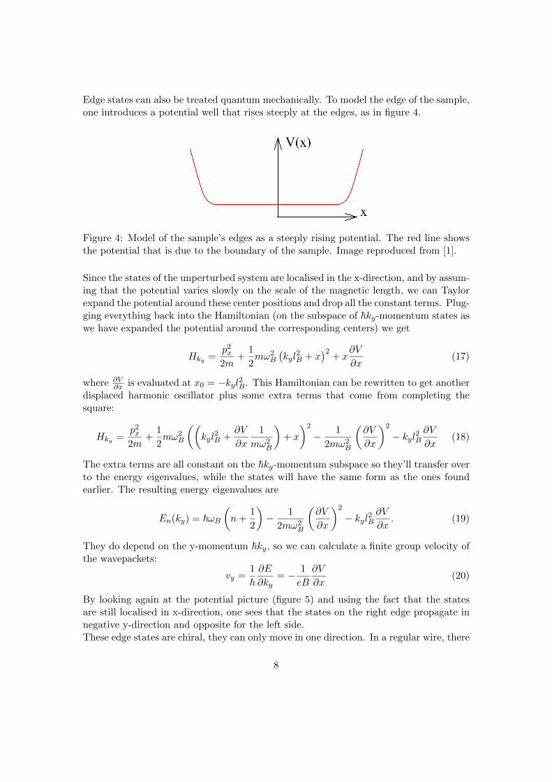
Edge states can also be treated quantum mechanically. To model the edge of the sample,one introduces a potential well that rises steeply at the edges, as in figure 4.

Figure 4: Model of the sample’s edges as a steeply rising potential. The red line showsthe potential that is due to the boundary of the sample. Image reproduced from [1].

Since the states of the unperturbed system are localised in the x-direction, and by assum-ing that the potential varies slowly on the scale of the magnetic length, we can Taylorexpand the potential around these center positions and drop all the constant terms. Plug-ging everything back into the Hamiltonian (on the subspace of ~ky-momentum states aswe have expanded the potential around the corresponding centers) we get

Hky =p2x

2m+

1

2mω2

B

(kyl

2B + x

)2+ x

∂V

∂x(17)

where ∂V∂x is evaluated at x0 = −kyl2B. This Hamiltonian can be rewritten to get another

displaced harmonic oscillator plus some extra terms that come from completing thesquare:

Hky =p2x

2m+

1

2mω2

B

((kyl

2B +

∂V

∂x

1

mω2B

)+ x

)2

− 1

2mω2B

(∂V

∂x

)2

− kyl2B∂V

∂x(18)

The extra terms are all constant on the ~ky-momentum subspace so they’ll transfer overto the energy eigenvalues, while the states will have the same form as the ones foundearlier. The resulting energy eigenvalues are

En(ky) = ~ωB(n+

1

2

)− 1

2mω2B

(∂V

∂x

)2

− kyl2B∂V

∂x. (19)

They do depend on the y-momentum ~ky, so we can calculate a finite group velocity ofthe wavepackets:

vy =1

~∂E

∂ky= − 1

eB

∂V

∂x(20)

By looking again at the potential picture (figure 5) and using the fact that the statesare still localised in x-direction, one sees that the states on the right edge propagate innegative y-direction and opposite for the left side.These edge states are chiral, they can only move in one direction. In a regular wire, there

8

are electrons that move to the right and ones that move to the left. These right-moversand left-movers can coexist in the same spatial region. Upon reversing time right-moversbecome left-movers and vice-versa. Since they are in the same spatial region, the systemlooks the same. For the system here, the right-movers are spatially separated from theleft-movers. Time reversal thus returns a system that looks like a mirror-image of theoriginal system, it looks reversed. This asymmetry is due to the presence of the magneticfield.

Figure 5: Model of the sample’s edges as a steeply rising potential, where the states belowthe Fermi level EF are occupied. Blue circles model the centers of the wavefucntions ofthe occupied states. Image reproduced from [1].

By introducing an electro-chemical potential difference ∆µ between the two edges, wecan calculate the arising current Iy:

Iy = − e

Ly

∫dky

Ly2πvy(ky) =

e

2πl2B

∫dx

1

eB

∂V

∂x=

e

2π~∆µ (21)

where we assumed one completely filled Landau level for the integration. By noting thatthe Hall voltage VH across the sample is given by the potential difference, one finds thatthe Hall conductivity takes the value of the first plateau level:

VH =∆µ

e⇒ σxy =

IyVH

=e2

2π~(22)

The argument can be expanded for multiple filled Landau levels and one will get thecorresponding conductivities of the plateaux.As a side note, the potential introduced before does not have to be flat in the centerregion, it can be as random as it wants to be (see figure 6) as long as we can make thesame arguments for the expansion as before. The resulting Hall current will be the samein any case.

There is another interesting property of the edge states; they are immune to back-scattering by impurities. In the classical picture, defects and impurities scatter incomingelectrons into random directions, effectively decreasing the current. Quantum mechan-ically, the electron always has to occupy a state, so it can only be scattered in one of

9

the non-populated states. In our system, these states live above the Fermi level, see theempty black circles in figure 6. If an edge state is scattered into a state right above itself,the resulting Hall current will be the same. If it would scatter on to the other side of thesample, the net current would change. However, the width of the sample is macroscopic,so such scattering is highly suppressed. The Hall current carried by the edge states istherefore immune to back-scattering.

Figure 6: Model of the sample’s edges as a steeply rising potential, where the middlepart seems random. The empty black circles denote unoccupied states right above theFermi level. Image reproduced from [1].

The above argument might look convincing, but it does not give any reason as to whythe conductivity is stable against change in the magnetic field. To see this, we needsomething else, we need to add disorder to our system. We will see that disorder isessential for the integer quantum Hall effect.

2.2 The Role of Disorder

Experimentally, there is always disorder in a system. But before we look at the effects ofdisorder, let us see what happens without it. In the absence of disorder, the Hall systemfeatures continuous translational invariance. In the lab frame, the fields are as follows

E = 0, B = Bez (23)

where the current density J is zero. Transforming to a Lorentz-boosted reference frame,where the boost is along the y-direction at speed v, the fields become the following:

E’ = γvBex ≈ vBex, B’ = γBez ≈ Bez (24)

where γ ≈ 1 is valid for small v. The transformed current densitiy is

J = nevey (25)

where the minus sign due to the Lorentz boost cancelled the one coming from the negativecharge of the electrons. The electric field expressed in terms of the current densitybecomes

E =1

neJ×B⇒

(ExEy

)=B

ne

(0 1−1 0

)(JxJy

)(26)

10

so the resulting resistivities and conductivities are

ρxx = 0, ρxy =B

ne, σxx = 0, σxy =

ne

B(27)

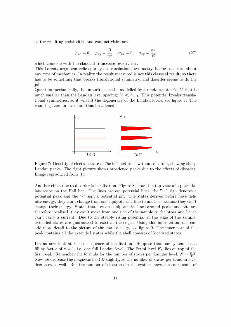
which coincide with the classical transverse resistivities.This Lorentz argument relies purely on translational symmetry, it does not care aboutany type of mechanics. In reality the result measured is not this classical result, so therehas to be something that breaks translational symmetry, and disorder seems to do thejob.Quantum mechanically, the impurities can be modelled by a random potential V that ismuch smaller than the Landau level spacing: V � ~ωB. This potential breaks transla-tional symmetries, so it will lift the degeneracy of the Landau levels, see figure 7. Theresulting Landau levels are thus broadened.

Figure 7: Densitiy of electron states. The left picture is without disorder, showing sharpLandau peaks. The right picture shows broadened peaks due to the effects of disorder.Image reproduced from [1].

Another effect due to disorder is localisation. Figure 8 shows the top-view of a potentiallandscape on the Hall bar. The lines are equipotential lines, the ”+” sign denotes apotential peak and the ”-” sign a potential pit. The states derived before have defi-nite energy, they can’t change from one equipotential line to another because they can’tchange their energy. States that live on equipotential lines around peaks and pits aretherefore localised, they can’t move from one side of the sample to the other and hencecan’t carry a current. Due to the steeply rising potential at the edge of the sample,extended states are guaranteed to exist at the edges. Using this information, one canadd more detail to the picture of the state density, see figure 9. The inner part of thepeak contains all the extended states while the shell consists of localised states.

Let us now look at the consequence of localisation. Suppose that our system has afilling factor of ν = 1, i.e. one full Landau level. The Fermi level EF lies on top of thefirst peak. Remember the formula for the number of states per Landau level, N = BA

Φ0.

Now we decrease the magnetic field B slightly, so the number of states per Landau leveldecreases as well. But the number of electrons in the system stays constant, some of

11

them have to populate states in a higher Landau level. The Fermi level E′F jumps intothe next region of states, which is a region of localised states in the next Landau level,see figure 9. These states however do not carry a current, they can’t contribute to theconductivity! The conductivity thus stays constant over a range of magnetic fields, itstays constant as long as the Fermi level lies in a region of localised states, a mobility gap.So disorder explains the stability to the magnetic field, it is essential to the whole effect.

Figure 8: Top view of the potential landscape. The lines are equipotential lines, theyform closed loops around peaks (”+” signs) and pits (”-” signs). Image reproduced from[1].

Figure 9: Densitiy of electron states. The outer parts in a Landau peak are localisedstates, where extended states live in the inner part. The Fermi level EF before thechange in magnetic field lies right at the top of the first Landau level, indicating a fillingfactor of 1. The Fermi level E′F after the change in the magnetic field lies in the regionof localised states in the second Landau level. Image reproduced from [1].

In the next step we will look at a more sophisticated argument as to why the conductivityis quantized in the values of σxy = e2

2π~ν, ν ∈ Z.

12

2.3 The Role of Gauge Invariance

The following argument relies on a different geometry that can be achieved by bendingthe Hall bar into a disk shape, called a Corbino ring, that is shown in figure 10. We arestill keeping the constant magnetic field going through the sample. We can introduce aflux Φ that goes through the hole in the disk, without affecting the magnetic field goingthrough the disk surface. Let us assume that this flux can be changed adiabatically,i.e. arbitrarily slowly. Faraday’s law then tells us that a change in flux induces anelectromotive force E . A radial current Ir would then allow us to calculate the Hallconductivity σH of the system, shown by the following equation:

E = −∂Φ/∂t = −∆Φ/T, Ir = ∆Qr/T → σH =IrE

(28)

where ∆Qr is the charge moved radially during the addition of a flux ∆Φ during a timeT .

Figure 10: The Corbino geometry, where the states live in the red ring that is penetratedby a uniform magnetic field. The blue tube models the addition of flux through the hole.Image reproduced from [1].

Now we will see that this radial current takes the appropriate values to get the correctHall conductivity. The system has rotational invariance (we are ignoring disorder forthe moment). By choosing the symmetric gauge, this symmetry is still apparent in theHamiltonian. Remember in the previous derivation of the eigenstates, the Hamiltonianhad translational invariance in the y-direction and we found plane waves in said direction.We also found harmonic oscillators in x-direction that were localised. By doing thecalculation for this Corbino geometry in the symmetric gauge, one finds again planewaves in azimuthal direction and harmonic oscillators in radial direction:

ψm,ν(~r) ∼ eimφfν(r − rm) (29)

where fν is a harmonic oscillator eigenfunction of the level ν+1 [2]. The center coordinate

rm is given by rm =√

2l2Bm that is now related to the angular momentum ~m as opposed

13

to the x0 coordinate being related to the y-momentum.Similar to the Aharonov-Bohm effect [1], adding one flux quantum leaves the systeminvariant. By adding this amount of flux adiabatically, one finds that the states increasetheir angular momentum by ~, they are mapped onto themselves. The center coordinatealso increases from rm to rm+1, so the states effectively move outwards. Because thesystem comes back to itself after the addition of one flux quantum, the number ofelectrons in our system stays the same. It started with an integer number of electrons soit ends with an integer number. Therefore exactly one electron per filled Landau level istransferred from the inner to the outer edge. The resulting Hall conductivity takes thevalues observed in the experiment:

∆Φ = Φ0 → ∆Qr = −ne, σH =ne

Φ0= n

e2

2π~, (30)

where n is the number of filled Landau levels. This argument involving the adiabaticchange in flux is called the Laughlin flux insertion argument, as Robert B. Laughlin firstcame up with this idea [3].We are now going to look at how disorder affects this argument. As seen before, disorderlocalises the states in the bulk but leaves extended states at the edge. The localised statesare not affected by the addition of flux as it can be removed by a gauge transformation.For extended states, this only works if the flux is an integer multiple of magnetic fluxquanta, because they have to obey a single-valuedness condition: By changing φ 7→ φ+2πthe state should remain unchanged. The extended states still undergo spectral flow andmap onto themselves under the adiabatic addition of integer number of flux quanta. Itis still guaranteed that at least two extended states exist per Landau level, one on eitheredge. As long as all the extended states in a Landau level are populated, threading oneflux quantum results in the radial current and the correct conductivity as we calculatedbefore. The extended states are populated as long as the Fermi level lies in a mobilitygap, which is possible due to the existence of disorder. Again, disorder and impuritiesare responsible for the stability of the Hall conductivity to changes in the magnetic field.

This completes the discussion of the integer quantum Hall effect within the edge picture.Parts of it are heuristic, but the role of gauge invariance hints that there may be a deeperconnection. In the next section, we are going to look at the bulk picture and we will findthat the integer quantum Hall effect appears as a consequence of a topological propertyof the Hall system.

14

3 The Bulk Picture

3.1 The Kubo Formula for Hall Conductivity

Before we can look at the topological property, we need to write the Hall conductivityin a different way, given by the Kubo formula. A full derivation of the Kubo formulacan be found in D. Tong’s lecture notes about the quantum Hall effect [1]. Here, only arough sketch of the derivation will be given.One starts with a multi-particle Hamiltonian H0 for a generic system that does not in-clude an electric field. We assume that we can solve this system, i.e. we know eigenstates|m〉 and eigenvalues Em such that H0 |m〉 = Em |m〉. We then introduce a weak electricfield E = −∂tA as a perturbation; ∆H = −J ·A, where J is the current operator. Ourgoal is to calculate the expectation value of the current operator 〈Jx〉 for the system inthe non-degenerate ground state |0〉. It is convenient to work in the interaction pictureand expand the expression for 〈Jx〉 up to linear order in ∆H. Comparing this new ex-pression with Ohm’s law Jx = σxxEx + σxyEy, one can filter out a formula for σxy. Theprecise derivation is part of a bigger story called linear response, but we are not goingdeeper into this. As a result, the expression for the Hall conductivity becomes

σxy = i~

LxLy

∑n 6=0

〈0 | Jy |n〉 〈n | Jx | 0〉 − 〈0 | Jx |n〉 〈n | Jy | 0〉(En − E0)2 . (31)

This is the Kubo formula for Hall conductivity. The sum runs over all the excited multi-particle states, inside there are transition amplitudes from excited states over the currentoperators to the ground state, weighted by the energy difference of these states. So ifone can solve the unperturbed system, this formula instantly gives an expression for theHall conductivity of that system.In the next section we will see a how a topological property leads to the quantisation ofthe Hall conductivity.

3.2 Hall System on a Torus

For this section, we have to modify the geometry again. This time, the Hall bar is bentinto a torus, which is a rectangle with opposite edges identified. The system is now madefully periodic, all edges have been removed, so there are no more edge states. There isstill a homogeneous magnetic field perpendicular to the torus’ surface. (Note it is athought experiment. In an actual experiment, this non-zero magnetic flux through aclosed surface would require magnetic monopoles.)

15

Figure 11: The Hall system on a torus. The red and blue shapes indicate two differentfluxes that can be added to the system. Image reproduced from [1].

Now we expand Laughlin’s flux threading argument: One can now insert two fluxes, onethrough either hole of the torus, as in figure 11. The Hamiltonian now depends on thesetwo fluxes, H = H(Φx,Φy). Similar to the previous case, the system’s spectrum is onlysensitive to the non-integer part of Φi/Φ0, i ∈ {x, y}. This time, there are no edges, noelectrons transfer from one side to another one. By the addition of one flux quantum,the system comes back to itself fully! Having zero flux is therefore the same as havingone flux quantum, which makes the space of parameters of the Hamiltonian periodic:

0 ≤ Φx < Φ0, 0 ≤ Φy < Φ0 (32)

This describes a torus T2Φ, the parameter space of our system is toroidal. Let us now

calculate the system’s Hall conductivity.Let H0 describe the unperturbed system. Treat the addition of flux as a perturbation∆H given by

∆H = −∑i=x,y

JiΦi

Li(33)

where Lx and Ly are the dimensions of the system. One can now use first order pertur-bation theory to calculate the many particle ground state of the perturbed system:

∣∣ψ′0⟩ = |ψ0〉+∑n 6=ψ0

〈n |∆H |ψ0〉En − E0

|n〉 (34)

where |ψ0〉 is the non-degenerate ground state of the unperturbed system. Consider nowinfinitesimal changes in flux and see how the state changes:∣∣∣∣∂ψ′0∂Φi

⟩= − 1

Li

∑n 6=ψ0

〈n|Ji|ψ0〉En − E0

|n〉 (35)

16

The elements in this summation look similar to the Kubo formula, eq. (31)! One canactually rewrite the Kubo formula (and therefore the Hall conductivity) in terms of thesestates:

σxy = i~[⟨

∂ψ′0∂Φy

∣∣∣∣ ∂ψ′0∂Φx

⟩−⟨∂ψ′0∂Φx

∣∣∣∣ ∂ψ′0∂Φy

⟩](36)

This expression can be rewritten by pulling out one derivative for each one of the brakets,becoming

σxy = i~[∂

∂Φy

⟨ψ′0

∣∣∣∣ ∂ψ′0∂Φx

⟩− ∂

∂Φx

⟨ψ′0

∣∣∣∣ ∂ψ′0∂Φy

⟩]. (37)

This however looks similar to the field strength of a Berry connection. Let us firstparameterise the torus using the dimensionless variables

θi =2πΦi

Φ0, θi ∈ [0, 2π) . (38)

Now, the Berry connection [1] is defined as

Ai(Φ) = −i⟨ψ′0

∣∣∣∣ ∂∂θi∣∣∣∣ψ′0⟩ . (39)

The field strength, or curvature of the Berry connection is the curl of the connection:

Fxy =∂Ax∂θy

− ∂Ay∂θx

= −i[∂

∂θy

⟨ψ′0

∣∣∣∣ ∂ψ′0∂θx

⟩− ∂

∂θx

⟨ψ′0

∣∣∣∣ ∂ψ′0∂θy

⟩](40)

This term looks pretty much the same as our expression for the conductivity, eq (37).The difference that in one case, the derivatives are with respect to θi instead of Φi, givesthe right constants. As a result, the conductivity is given by the curvature:

σxy = −e2

~Fxy (41)

This does not tell us much yet. However if one averages this expression over all fluxesin the toroidal parameter space T2

Φ, one gets a more interesting result:

σxy = − e2

2π~

∫T2

Φ

dθ

2πFxy = − e2

2π~C (42)

where ∫T2

Φ

dθ

2πFxy = C ∈ Z (43)

is the first Chern number, and it is always an integer [7].This result is the topological argument we have been looking for. The Hall conductivityis a Chern number, it can’t continuously change. It is therefore invariant under smallchanges of the Hamiltonian, which would result in small changes of the Berry curva-ture. One would always expect a graph of Chern numbers to form plateaux. Large

17

deformations correspond to energy level crossings, and our non-degeneracy assumptionbreaks down. This situation describes a transition between two Chern numbers, i.e. twoplateau levels in the conductivity.We have seen that for a system with continuous translational symmetry, a toroidal pa-rameter space led to the desired quantisation. However, we haven’t seen a reason as towhy one should average the conductivity over the parameter space, and I do not knowone either. It turns out that if one looks at particles on a lattice, the integral appearsnaturally, without taking any averages. Such a system was used originally to measurethe quantum Hall effect. It only features discrete translational invariance, so one mightexpect some things to go wrong. In the next sections, we are going to look at this moreclosely.

3.3 Particles on a Lattice

A lattice has a discrete periodicity given by the lattice vectors rn, and so does thecorresponding lattice potential. The energy spectrum of such a system forms bands.Due to Bloch’s theorem, we know that the wavefunctions in each band can be writtenin the Bloch form as

ψk(r) = eik·ruk(r), uk(r) = uk(r + rn), ψk+G(r) = ψk(r) (44)

where k is the lattice momentum and G is a reciprocal lattice vector. Most importantly,the wavefunction is periodic in the first Brillouin zone. For a rectangular lattice withlattice constants a and b, the Brillouin zone is rectangular as well. But a periodicrectangle is a torus, so our wavefunction is periodic on a toroidal space T2 of latticemomenta:

−πa< kx ≤

π

a, −π

b< ky ≤

π

b(45)

Let us now assume that the Fermi level EF lies in a gap between two energy bands,meaning that all the bands below the Fermi level are completely filled, and all the bandsabove are completely unoccupied. The Hamiltonian of such a system can be rewrittenusing Bloch’s theorem:

H |ψk〉 = Ek |ψk〉 ⇒ H(k) |uk〉 = Ek |uk〉 with H(k) = e−ik·xHeik·x (46)

The current operator is now given by

J =e

~∂H

∂k(47)

which is analogous to the more conventional J = −ex. The Kubo formula we have seenin section 3.1 can be rewritten in terms of single particle states. This is because allelectron-electron interactions are neglected, so a multi-particle state is just a product ofall the single-particle states. For states living in discrete energy bands with continuouslattice momenta, the Kubo formula becomes

σxy = i~∑

Eα<EF<Eβ

∫T2

d2k

(2π)2

〈uαk|Jy|uβk〉〈u

βk|Jx|u

αk〉 − 〈uαk|Jx|uαk〉〈uαk|Jy|uαk〉

(Eβ(k)− Eα(k))2 (48)

18

where the sum runs over all the energy bands and the integral runs over all the continuouslattice momenta in each band. By plugging the Ansatz for the current operator (47)into this Kubo formula, one gets

σxy =ie2

2π~∑α

∫T2

d2k

2π[〈∂yuαk|∂xuαk〉 − 〈∂xuαk|∂yuαk〉] . (49)

Let us now look at the following U(1) Berry connection, defined over T2:

Aαi (k) = −i⟨uαk

∣∣∣∣ ∂

∂ki

∣∣∣∣uαk⟩ (50)

The field strength associated to this connection is

Fαxy =∂Aαx∂ky

−∂Aαy∂kx

= −i[⟨

∂uα

∂ky

∣∣∣∣ ∂uα∂kx

⟩−⟨∂uα

∂kx

∣∣∣∣ ∂uα∂ky

⟩]. (51)

By integrating this field strength over the Brillouin zone T2, one obtains the first Chernnumber,

Cα =

∫T2

d2k

2πFαxy. (52)

By comparing equations (51) and (52) with the expression for the Hall conductivity (49),we get

σxy = − e2

2π~∑α

Cα, Cα ∈ Z. (53)

This is the TKNN formula, named after Thouless, Kohmoto, Nightingale and Nijs, whichare the people that came up with it [4]. It tells us that each isolated, filled band (labelledby α) contributes an integer part Cα to the Hall conductivity of the system. The set ofCα is sometimes called the TKNN integers. We have attributed this set of integers toa Hamiltonian, they define the Hall conductivity of the corresponding system. Similarto the case in section 3.2, this formula states that the Hall conductivity is a topologicalinvariant of the system. It is robust to small changes of the system as it can’t changecontinuously.We are going to see a more precise formulation of this statement in the end. Let us nowlook at an example, giving a hint at this more precise formulation.

3.3.1 Example: The Chern Insulator

The system we are looking at has two distinct energy bands and the Fermi level liesbetween them, meaning the system is insulating. Even though there is no magneticfield, this system can have a non-zero Chern number, hence the name Chern insulator.The system in k-space is modelled by a two-state Hamiltonian in the most general form,

H(k) = ~E(k) · ~σ + ε(k)1 (54)

19

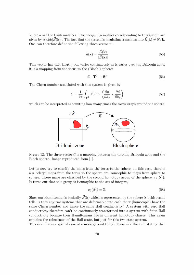
where ~σ are the Pauli matrices. The energy eigenvalues corresponding to this system aregiven by ε(k)±| ~E(k)|. The fact that the system is insulating translates into ~E(k) 6= 0∀k.One can therefore define the following three-vector ~n:

~n(k) =~E(k)

| ~E(k)|(55)

This vector has unit length, but varies continuously as k varies over the Brillouin zone,it is a mapping from the torus to the (Bloch-) sphere:

~n : T2 → S2 (56)

The Chern number associated with this system is given by

C =1

4π

∫T2

d2k ~n ·(∂~n

∂kx× ∂~n

∂ky

)(57)

which can be interpreted as counting how many times the torus wraps around the sphere.

Figure 12: The three-vector ~n is a mapping between the toroidal Brillouin zone and theBloch sphere. Image reproduced from [1].

Let us now try to classify the maps from the torus to the sphere. In this case, there isa subtlety: maps from the torus to the sphere are isomorphic to maps from sphere tosphere. These maps are classified by the second homotopy group of the sphere, π2(S2).It turns out that this group is isomorphic to the set of integers,

π2(S2) = Z. (58)

Since our Hamiltonian is basically ~E(k) which is represented by the sphere S2, this resulttells us that any two systems that are deformable into each other (homotopic) have thesame Chern number and hence the same Hall conductivity! A system with zero Hallconductivity therefore can’t be continuously transformed into a system with finite Hallconductivity because their Hamiltonians live in different homotopy classes. This againexplains the robustness of the Hall-state, but just for this two-state system.This example is a special case of a more general thing. There is a theorem stating that

20

two maps from the Brillouin zone to the space of gapped hermitian matrices (Hamilto-nians) are homotopic if and only if the they both have the same TKNN integers, andtherefore have the same Hall conductivity, see [5]. We will come back to this again insection 4.In the next section we are going to look how things change when we introduce a magneticfield. It is not obvious that the Brillouin zone survives this addition, so we might wantto check if the TKNN formula is still applicable.

3.4 Particles on a Lattice in a Magnetic Field

So far we haven’t included a magnetic field into our discussion about particles on alattice. In the experiment, this has been done, and from the edge picture we know thata magnetic field is crucial to the effect. The main goal of this treatment is to find azone where the states of the system are periodic, we want to find an analogue to theBrillouin zone. If we have that, one can simply apply the TKNN formula. It is notobvious that there exists such a magnetic Brillouin zone as the Hamiltonian loses thediscrete translational invariance of the lattice due to the vector potential arising fromthe magnetic field.Let us work in the tight-binding approximation and assume a square lattice with latticeconstant a. One can also find a Brillouin zone when working with a weak potentialand a non-square lattice, see [4]. In the tight-binding approximation, the states arelocalised around the lattice points. These position eigenstates |x〉 are discrete, they arerestricted to x = a(m,n) with m,n ∈ Z. The Hamiltonian is discrete as well. Forthis approximation of a strong potential, the Hamiltonian allows states to hop from onelattice site to an adjacent one. It is given by

H = −t∑x

∑j=1,2

|x〉 〈x + ej | − t∗∑x

∑j=1,2

|x + ej〉 〈x| (59)

with e1 = (a, 0), e2 = (0, a) and t being the probability amplitude for hopping to occur.The on-site energy has been set to zero, it is just an additive constant to the Hamiltonian.Now we can add a magnetic field to the system,

Bz = ∇×A. (60)

Intuitively, a vector potential is part of the canonical momentum p. Canonical momen-tum is the rate at which the phase of a state changes, per unit length. For our set ofdiscrete states, this length is fixed at a. So the change in the Hamiltonian is just a phase,its new form is

H = −t∑x

∑j=1,2

|x〉 e−ieaAj(x)/~ 〈x + ej |+ h.c., (61)

which has no discrete translational invariance anymore. This Hamiltonian should betterbe compatible with the Aharonov-Bohm effect, and indeed it is. Let us take a state andmove it once around a unit cell (see figure 13), it will pick up a phase of e−iγ . This γ

21

can be calculated from the form of the Hamiltonian, and it is

γ =ea

~(A1(x) +A2(x+ e1)−A1(x+ e2)−A2(x)) ≈ ea

~

(∂A2

∂x1− ∂A1

∂x2

)(62)

where in the second step, we have approximated finite differences with actual derivatives(remember our space coordinate is discretised). But the expression in the bracket is justthe curl of the vector potential, so

γ ≈ ea

~

(∂A2

∂x1− ∂A1

∂x2

)=ea2B

~(63)

where a2B is the magnetic flux through the unit cell, so this really is the Aharonov-Bohmphase.

Figure 13: Schematic view of the square lattice. A state moving along a lattice sitepicks up a phase proportional to the vector potentials written above each line. Imagereproduced from [1].

Now that we have a Hamiltonian, we want to find eigenstates and eigenvalues. Our goalis to find operators that commute with the Hamiltonian and then to find a common setof eigenstates. Let us define the modified magnetic translation operators:

Tj =∑x

|x〉 e−ieaAj(x)/~ 〈x + ej | (64)

The Aj is not the same vector potential as before, but it fulfils ∂kAj = ∂jAk. Theseoperators have the following commutation relations:

[H, Tj ] = 0, T2T1 = eieΦ/~T1T2 (65)

The first commutation relation can be seen by introducing the usual magnetic translationoperator (which replaces Aj by Aj). The Hamiltonian is then given by a superpositionof these operators, and they commute with their modified counterparts. The secondrelation we don’t like quite as much yet. It would be nicer if [T1, T2] were zero as well,because in that case one could find simultaneous eigenstates of all three operators. Forthis to happen we need to take the flux per unit cell to be a rational multiple of the flux

22

quantum: Ba2 = Φ = pqΦ0, with p, q integers that are relatively prime. Then, one can

rise the modified magnetic translation operators to an appropriate power and one gets

[Tn11 , Tn2

2 ] = 0 (66)

whenever pqn1n2 ∈ Z, in particular for n1 = q, n2 = 1. Of course they still commute

with the Hamiltonian. So a set of commuting operators is given by H, T q1 , T2 and wecan now move on to the eigenstates. Let us label these states by their magnetic latticemomentum k:

|k〉 , k = (k1, k2) (67)

The eigenvalue equations then become

H |k〉 = E(k) |k〉 , T q1 |k〉 = eiqk1a |k〉 , T2 |k〉 = eik2a |k〉 . (68)

We see that the ki are again periodic:

− π

qa< k1 ≤

π

qaand − π

a< k2 ≤

π

a(69)

The zone of periodicity is called the magnetic Brillouin zone, and it again forms a TorusT2! It is smaller by a factor of q compared to the conventional Brillouin zone. Thecorresponding unit cell (enlarged by a factor of q) contains p magnetic flux quanta.Finding the Brillouin zone hence boils down to finding a unit cell containing an integernumber of magnetic flux quanta! The number of states per magnetic Brillouin zone isgiven by L1L2/qa

2. This suggests that the energy spectrum decomposes into q bands.Now we look at the degeneracy of the states. Let us pay closer attention to the stateT1 |k〉 which is not an eigenstate of T1. From the calculations before, we know that T1

commutes with the Hamiltonian, [H, T1] = 0. We have

HT1 |k〉 = E(k) |k〉 , T2T1 |k〉 = eieΦT1T2 |k〉 = ei(2πp/q+k2a)T1 |k〉 . (70)

From equation (68) we know that T2 |k〉 = eik2a |k〉, so

T1 |k〉 ∼ |(k1, k2 + 2πp/qa)〉 (71)

and it also has the same energy as |(k1, k2)〉. This results in a q-fold degeneracy in agiven band. One can now go on and calculate the energy eigenvalues and the Chernnumbers. However, one might expect to run into some issues, as each isolated band hasto contribute an integer number of e2

2π~ to the Hall conductivity, and the number of bandsq can become arbitrarily large by changing the magnetic flux Φ by an arbitrarily smallamount. Also, if the flux is given by an irrational multiple of Φ0, the above calculationdoesn’t work out and the spectrum of the Hamiltonian forms a Cantor set. But theexperiment shows the conductivity to remain constant over a range of magnetic flux, norapid behaviour is observed. Nontheless, the calculation works out, but it is not givenhere as it is rather complicated. It can be found in the original TKNN paper [4] and inthe book Field Theories of Condensed Matter Physics by Fradkin [8].

23

Now we have all that we need to apply the TKNN formula (53): There exists a toroidalBrillouin zone and the spectrum decomposes into bands. As a result, the system has aquantised Hall conductivity. So we found the quantised conductivity for the Hall systemin a picture without edges! This concludes the discussion of the integer quantum Halleffect within the bulk picture.

4 Conclusion

Now that we have found the quantised conductivity in the lattice model, one might askwhat exactly the topological property of the Hall system is. There is a theorem [5] thatanswers this question, it was briefly mentioned in section 3.3.1. It goes as follows: LetH1(k), H1(k): T2 → [space of Hamiltonian matrices] be two maps from the (magnetic)Brillouin zone (which is toroidal) to the space of gapped, periodic, hermitian matrices,i.e. Hamiltonians that describe the system, the band structure. Then, these two mapsare continuously deformable into each other (homotopic) if and only if they have thesame TKNN integers. Remember the TKNN formula giving the Hall conductivity forsuch a system,

σxy = − e2

2π~∑α

Cα, Cα ∈ Z. (72)

This theorem tells us, that if two systems are continuously deformable into each other,they have the same Hall conductivity. If they have different Chern numbers (and hencea different conductivity), they are not deformable into each other, they live in differenthomotopy classes. It also shows us that the topological property lies in the connectionbetween the Brillouin zone and the band structure (which is H(k)).At the same time, we found a quantised Hall conductivity in the edge picture. Theseedge modes are the counterpart to the quantised conductivity, their robustness is dueto this topological property of the Hamiltonian. The topology is physically manifest inthe number of protected edge modes of the system. The edge modes exist because ofthe topological indices of the system, the TKNN integers. This correspondence is alsoknown as the bulk-edge correspondence.

24

References

[1] D. Tong, ”The Quantum Hall Effect”, arXiv:1606.06687.

[2] B.I. Halperin, ”Quantized Hall conductance, current-carrying edge states, and theexistence of extended states in a two-dimensional disordered potential”, Phys. Rev.B 25, 2185 (1982).

[3] R.B. Laughlin, ”Quantized Hall conductivity in two dimensions”, Phys. Rev. B 23,5632 (1981).

[4] D.J. Thouless, M. Kohmoto, M. Nightingale, M. den Nijs, ”Quantized Hall Conduc-tance in a Two-Dimensional Periodic Potential”, Phys. Rev. Lett. 49, 405 (1982).

[5] J.E. Avron, R. Seiler, B. Simon, ”Homotopy and Quantization in Condensed MatterPhysics”, Phys. Rev. Lett. 51, 51 (1983).

[6] The University of Manchester, ”Advanced Quantum Mechanics 2” [Online],http://oer.physics.manchester.ac.uk/AQM2/Notes/Notes-4.4.html

[7] N. Manton, P. Sutcliffe, ”Topological Solitons”, Cambridge University Press (2004).

[8] E. Fradkin, ”Field Theories of Condensed Matter Physics”, University of Illinois(2013).

25