instrumentation and communication lab
DESCRIPTION
Instrumentation And Communication lab practical file for NIT Kurukshetra.TRANSCRIPT

Practical File
INSRUMENTATION AND CONTROL LAB
Submitted By
INDEX
Sr no Name of the Experiment Exp date Submission date Remarks
Experiment Number 3AIM Introduction to LabVIEW software and its bases
APPARATUS Computer system compatible with LabVIEW
THEORYLabVIEW (short for Laboratory Virtual Instrumentation Engineering Workbench) is a platform and development environment for a visual programming language from National Instruments The graphical language is named G LabVIEW is commonly used for data acquisition instrument control and industrial automation on a variety of platforms including Microsoft Windows various flavors of UNIX Linux and Mac OS
One benefit of LabVIEW over other development environments is the extensive support for accessing instrumentation hardware Drivers and abstraction layers for many different types of instruments and buses are included or are available for inclusion These present themselves as graphical nodes The abstraction layers offer standard software interfaces to communicate with hardware devices The provided driver interfaces save program development time Many libraries with a large number of functions for data acquisition signal generation mathematics statistics signal conditioning analysis etc along with numerous graphical interface elements are provided in several LabVIEW package options Another benefit of the LabVIEW environment is the platform independent nature of the G‐code (LabVIEW programming language) which is (with the exception of a few platform‐specific functions) portable between the different LabVIEW systems for different operating systems (Windows MacOSX and Linux)Graphical programmingLabVIEW ties the creation of user interfaces (called front panels) into the development cycle LabVIEW programssubroutines are called virtual instruments (VIs) Each VI has three components Each VI contains three main parts
1Front Panel ‐ How the user interacts with the VI2Block Diagram ‐ The code that controls the program3IconConnector ‐ Means of connecting a VI to other VIs
The Front Panel is the user interface of the VI to interact with the user when the program is running Users can control the program change inputs and see data updated in real time You build the front panel with controls and indicators (available on the Control Palette) which are the interactive input and output terminals of the VI respectively Controls are knobs pushbuttons dials and other input devices Indicators are graphs LEDs and other displays Controls simulate instrument input devices and supply values to the block diagram of the VI
Indicators simulate instrument output devices and display values the block diagram acquires or generates These may include data program states and other information Every front panel control or indicator has a corresponding terminal on the block diagram When a VI is run values from controls flow through the block diagram where they are used in the functions on the diagram and the results are passed into other functions or indicators
The Controls palette is available only on the front panel Go to WindowraquoShow Controls Palette or right‐click the front panel workspace to display the Controls palette
The Functions palette is available only on the block diagram Select WindowraquoShow Functions Palette or right‐click the block diagram workspace to display the Functions palette
The Block Diagram contains this graphical source code Front panel objects appear as terminals on the block diagram Additionally the block diagram contains functions and structures from built‐in LabVIEW VI libraries These can be accessed from the Functions Palette Wires connect each of the nodes on the block diagram including control and indicator terminals functions and structuresThe IconConnector may represent the VI as a subVI in block diagrams of calling VIs Controls and indicators on the front panel allow an operator to input data into or extract data from a running virtual instrument However the front panel can also serve as a programmatic interface Thus a virtual instrument can either be run as a program with the front panel serving as a user interface or when dropped as a node onto the block diagram the front panel defines the inputs and outputs for the given node through the connector pane This implies each VI can be easily tested before being embedded as a subroutine into a larger program
The graphical approach also allows non‐programmers to build programs by simply dragging and dropping virtual representations of the lab equipment with which they are already familiar The LabVIEW programming environment with the included examples and the documentation makes it easy to create small applications For complex algorithms or large‐scale code it is important that the programmer possess an extensive knowledge of the special LabVIEW syntax and the topology of its memory management The most advanced LabVIEW development systems offer the possibility of building stand‐alone applications
Other features that you will need include the Tools Palette which is a Floating Palette that is used to operate and modify front panel and block diagram objects and the Status Toolbar They contain the following tools and buttons respectively
Tools Palette
Status Bar
Exercise 1- Convert oC to oF
Complete the following steps to create a VI that takes a number representing degrees Celsius and converts it to a number representing degrees Fahrenheit
In wiring illustrations the arrow at the end of this mouse icon shows where to click and the number on the arrow indicates how many times to click
Front Panel1 Select Fileraquo New to open a new front panel
2 (Optional) Select WindowraquoTile Left and Right to display the front panel and block diagram side by side
3 Create a numeric digital control You will use this control to enter the value for degrees Centigrade
aSelect the digital control on the ControlsraquoNumeric Controls palette If the Controls palette is not visible right‐click an open area on the front panel to display it
bMove the control to the front panel and click to place the controlcType deg C inside the label and click outside the label or click the Enter button
on the toolbar If you do not type the name immediately LabVIEW uses a default label You can edit a label at any time by using the Labeling tool
4 Create a numeric digital indicator You will use this indicator to display the value for degrees Fahrenheit
aSelect the digital indicator on the ControlsraquoNumeric Indicators palettebMove the indicator to the front panel and click to place the indicatorcType deg F inside the label and click outside the label or click the Enter button
LabVIEW creates corresponding control and indicator terminals on the block diagram The terminals represent the data type of the control or indicator For example a DBL terminal represents a double‐ precision floating‐point numeric control or indicator
Note Control terminals have a thicker border than indicator terminals
Block Diagram5 Display the block diagram by clicking it or by selecting WindowraquoShow Diagram
Note Block Diagram terminals can be viewed as icons or as terminals To change the way LabVIEW displays these objects right click on a terminal and select View As Icon
6Select the Multiply and Add functions on the Functionsraquo Numeric palette and place them on the block diagram If the Functions palette is not visible right‐click an open area on the block diagram to display it
7Select the numeric constant on the Functionsraquo Numeric palette and place two of them on the block diagram When you first place the numeric constant it is highlighted so you can type a value
8Type 18 in one constant and 320 in the other If you moved the constants before you typed a value use the Labeling tool to enter the values
9Use the Wiring tool to wire the icons as shown in the previous block diagramTo wire from one terminal to another use the Wiring tool to click the first
terminal move the tool to the second terminal and click the second terminal as shown in the following illustration You can start wiring at either terminal
You can bend a wire by clicking to tack the wire down and moving the cursor in a perpendicular direction Press the spacebar to toggle the wire direction
To identify terminals on the nodes right‐click the Multiply and Add functions and select Visible ItemsraquoTerminals from the shortcut menu to display the connector pane Return to the icons after wiring by right‐clicking the functions and selecting Visible Itemsraquo
Terminals from the shortcut menu to remove the checkmarkWhen you move the Wiring tool over a terminal the terminal area blinks
indicating that clicking will connect the wire to that terminal and a tip strip appears listing the name of the terminal
To cancel a wire you started press the ltEscgt key right‐click or click the source terminal
10Display the front panel by clicking it or by selecting WindowraquoShow Panel11Save the VI for later use (have a folder by your own name)12Enter a number in the digital control and run the VI
aUse the Operating tool or the Labeling tool to double‐click the digital control and type a new number
bClick the Run button to run the VIcTry several different numbers and run the VI again
Exercise 2 ndash Create a SubVI
Front Panel1 Select FileraquoOpen and navigate to your folder to open the C to F VI The following front panel appears
2Right‐click the icon in the upper right corner of the front panel and select Edit Icon from the shortcut menu The Icon Editor dialog box appears
3Double‐click the Select tool on the left side of the Icon Editor dialog box to select the default icon
4Press the ltDeletegt key to remove the default icon5Double‐click the Rectangle tool to redraw the border6Create the following icon
aUse the Text tool to click the editing area
bType C and FcDouble‐click the Text tool and change the font to Small FontsdUse the Pencil tool to create the arrow (To draw horizontal or vertical
straight lines press the ltShiftgt key while you use the Pencil tool to drag the cursor)
eUse the Select tool and the arrow keys to move the text and arrow you created
fSelect the BampW icon and select 256 Colors in the Copy from field to create a black and white icon which LabVIEW uses for printing unless you have a color printer
gWhen the icon is complete click the OK button to close the Icon Editor dialog box The icon appears in the upper right corner of the front panel and block diagram
7Right‐click the icon on the front panel and select Show Connector from the shortcut menu to define the connector pane terminal pattern
LabVIEW selects a connector pane pattern based on the number of controls and indicators on the front panel For example this front panel has two terminals deg C and deg F so LabVIEW selects a connector pane pattern with two terminals
8Assign the terminals to the digital control and digital indicator
a Select HelpraquoShow Context Help to display the Context Help window View each connection in the Context Help window as you make it
bClick the left terminal in the connector pane The tool automatically changes to the Wiring tool and the terminal turns black
cClick the deg C control The left terminal turns orange and a marquee highlights the control
dClick an open area of the front panel The marquee disappears and the terminal changes to the data type color of the control to indicate that you connected the terminal
eClick the right terminal in the connector pane and click the deg F indicator The right terminal turns orange
fClick an open area on the front panel Both terminals are orangegMove the cursor over the connector pane The Context Help window shows
that both terminals are connected to floating‐point values9 Select FileraquoSave to save the VI
Exercise 3 ndash Using LoopsUse a while loop and a waveform chart to build a VI that demonstrates software timing
Front Panel
1Open a new VI2Build the following front panel
aSelect the horizontal pointer slide on the Controlsraquo Numeric Controls palette and place it on the front panel You will use the slide to change the software timing
bType millisecond delay inside the label and click outside the label or click the Enter button on the toolbar shown at left
cPlace a Stop Button from the ControlsraquoButtons palettedSelect a waveform chart on the ControlsraquoGraph Indicators palette and place it
on the front panel The waveform chart will display the data in real timeeType Value History inside the label and click outside the label or click the
Enter buttonfThe waveform chart legend labels the plot Plot 0 Use the Labeling tool to triple‐
click Plot 0 in the chart legend type Value and click outside the label or click the Enter button to relabel the legend
gThe random number generator generates numbers between 0 and 1 in a classroom setting you could replace this with a data acquisition VI Use the Labeling tool
to double‐click 100 in the y‐axis type 1 and click outside the label or click the Enter button to rescale the chart
hChange ndash100 in the y‐axis to 0iLabel the y‐axis Value and the x‐axis Time (sec)
Block Diagram
3Select WindowraquoShow Diagram to display the block diagram
4Enclose the two terminals in a While Loop as shown in the following block diagram
aSelect the While Loop on the FunctionsraquoExecution Control palettebClick and drag a selection rectangle around the two terminalscUse the Positioning tool to resize the loop if necessary
5Select the Random Number (0‐1) on the FunctionsraquoArithmetic and ComparisonraquoNumeric palette Alternatively you could use a VI that is gathering data from an external sensor
6Wire the block diagram objects as shown in the previous block diagram7Save the VI as Use a Loopvi in your folder8Display the front panel by clicking it or by selecting WindowraquoShow Panel9Run the VI The section of the block diagram within the While Loop border executes
until the specified condition is TRUE For example while the STOP button is not pressed the VI returns a new number and displays it on the waveform chart
10Click the STOP button to stop the acquisition The condition is FALSE and the loop stops executing
11Format and customize the X and Y scales of the waveform chartaRight‐click the chart and select Properties from the shortcut menu The
following dialog box appearsbClick the Scale tab and select different styles for the y‐axis You also can select
different mapping modes grid options scaling factors and formats and precisions Notice that these will update interactively on the waveform chart
cSelect the options you desire and click the OK button
12 Right‐click the waveform chart and select Data OperationsraquoClear Chart from the shortcut menu to clear the display buffer and reset the waveform chart If the VI is running you can select Clear Chart from the shortcut menu
Adding TimingWhen this VI runs the While Loop executes as quickly as possible Complete the following steps to take data at certain intervals such as once every half‐second as shown in the following block diagram
aPlace the Time Delay Express VI located on the FunctionsraquoExecution Control palette In the dialog box that appears insert 05 This function would make sure that each iteration occurs every half‐second (500 ms)
bDivide the millisecond delay by 1000 to get time in seconds Connect the output of the divide function to the Delay Time (s) input of the Time Delay Express VI This will allow you to adjust the speed of the execution from the pointer slide on the front panel
13Save the VI because you will use this VI later in the course14Run the VI15Try different values for the millisecond delay and run the VI again Notice how this
effects the speed of the number generation and display
EXPERIMENT NUMBER 2AIM To Study different transducers and their characteristics (LVDT strain gauge airflow humidity etc on the DIGIAC 1750)
APPARATUS DIGIAC 1750 kit connecting wires multimeter
THEORY
LINEAR POSITION OR FORCE APPLICATIONS
The Linear Variable Differential Transformer (LVDT)The construction and circuit arrangement an LVDT are as shown in Fig 41 It consists of three coils mounted on a common former and having a magnetic core that is movable within the coils
Figure 1 construction and circuit arrangement of LVDT
The center coil is the primary and is supplied from an AC supply The coils on either side are secondary coils and are labeled A amp B in Fig 41 Coils A amp B have equal number of turns and are connected in series opposing so that the output voltage is the difference between voltages induced in the coils
Fig 2 shows the output obtained for different positions of the magnetic core
Figure 2 output obtained for different positions of the magnetic core
With the core in its central position as shown in Fig 42(b) there should be equal voltages induced in coils A amp B by normal transformer action and the output voltage would be zero In practice this ideal condition is unlikely to be found but the output voltage will reduce to a minimum
With the core moved to the left as shown in Fig 42(a) the voltage induced in coil A (Va) will be greater than that induced in coil B (Vb) There will therefore be an output voltage Vout = (Va - Vb) and this voltage will be in phase with the input voltage as shown
With the core moved to the right as shown in Fig 42(c) the voltage induced in coil A (Va) will be less than that induced in coil B (Vb) and again there will be an output voltage Vout = (Va -Vb) but in this case the output voltage will be out of phase with the input voltage
Movement of the core from its central (or neutral) position produces an output voltage This voltage increases with the movement from the neutral position to a maximum value and then may reduce for further movement from this maximum setting Note that the phase will remain constant on either side of the neutral position There is no gradual change of phase only an abrupt reversal when passing through the neutral position
The Strain Gauge Transducer
Fig 3 construction of a strain gauge
Fig 3 shows the construction of a strain gauge consisting of a grid of fine wire or semiconductor material bonded to a backing material When in use the unit is glued to the beam under test and is arranged so that the variation in length under loaded conditions is along the gauge sensitive axis (Fig 45(a)) Loading the beam increases the length of the gauge wire and also reduces its cross-sectional area (Fig 45(c)) Both of these effects will increase the resistance of the wire
Fig4 The layout and circuit arrangement for the DIGIAC 1750
The layout and circuit arrangement for the DIGIAC 1750 unit is shown in Fig 4 Resistors are electro-deposited on a substrate on a contact block at the right-hand end of the
assembly The gauge is normally connected in a Wheatstone Bridge arrangement with the bridge balanced under no load conditions Any change of resistance due to loading unbalances the bridge and this is indicated by the detector (Galvanometer)
The Wheatstone Bridge circuit is liable to give inaccurate results due to thermal changes A variation of temperature will also produce a change of resistance of the gauge and this will be interpreted as a change of loading To correct for this an identical gauge is used and connected This gauge is placed near to the other gauge but is arranged so that it is not subjected to any loading Any variation of temperature now affects both gauges equally and there will be no thermal effect on the bridge conditions The gauge subjected to loading is referred to as the active gauge and the other is called the dummy gauge
The Humidity TransducerFig shows the construction of a humidity transducer consisting of a thin disc of a material whose properties vary with humidity Each side of the disc is metalized to form a capacitor
Variation of humidity of the surrounding air alters the permittivity andor thickness of the dielectric material changing the value of the capacitor The unit is housed in a perforated plastic case The unit is connected in series with a resistor with the output taken from the resistor With an alternating voltage applied to the input the output voltage will vary with humidity due to the variation of capacitance of the transducer
PROCEDURECharacteristics of a Linear Variable Differential Transformer
Figure 5
In this exercise we will measure the rectified output using the digital multinleter on the 20V DC range and also amplify and measure it using the MC analog meter as this gives a better impression of the variation of output voltage with core position
1 The circuit is connected as shown in Fig 5 with the digital multimeter on the 2V DC range to monitor the output of the Full-Wave Rectifier The power supply is turned ON
2 The AC Amplifier gain is set to 10003 The GAIN COARSE control of Amplifier 1 is set to 100 and GAIN FINE control to
02 The OFFSET control is checked that it is set for zero output with zero input and adjusted if necessary
4 The core position is adjusted by rotating the operating screw to the neutral position This will give minimum output voltage The value of this voltage is observed from the digital multimeter and it is recorded in Table
5 The core control screw is rotated in steps of 1 turn for 4 turns in the clockwise direction (when viewing the control from the left-hand side of the D1750 unit) and the results are recorded in Table Then the control screw is turned in the counter clockwise direction again recording the results in Table
6 Plot the graph of output voltage from the analog meter readings against core position is plotted
Figure 6
7 The circuit is changed to the circuit shown in Fig 6 to observe the effect of the polarity change in the output Note that test points are provided at the bottom of the DIGIAC 1750 Trainer panel for connection of oscilloscope probes
8 Note that for the L VDT considered here unless the two secondary coils are identical there will be non-perfect coupling between each secondary coil and the primary coil resulting in a frequency-dependent phase shift in the output voltage (relative to the input voltage)
9 Set up the oscilloscope as follows lock the time base to CH1 trigger selector to AC CH1 Amplifier on AC input 50mVdiv CH2 Amplifier on AC input 05Vdiv time base to 5usdiv
10 Both traces are positioned on the center horizontal line of the display11 The power supply is turned ON and the core position is varied through its full range
and the effect on the output voltage as seen on CH2 of the oscilloscope display is observed
12 Timebase fine control is adjusted to give 1frac12 cycles of displayed waveform 13 The oscilloscope waveform is sketched when the core is turned 2 turns in (+2) from
the neutral position on the graticule provided
Characteristics of a strain Gauge Transducer
Figure 7
1 Connect the circuit is connected as shown in Fig 7 and Amplifier 1 GAIN COARSE control is set to 100
2 The power supply is switched ON and with no load on the strain gauge platform the offset control of Amplifier 1 is adjusted so that the output voltage is zero
3 All ten of the weights is placed on the load platform and the GAIN FINE control is adjusted to give an output voltage of 70V as indicated on the moving coil meter
4 Note that this value of output voltage should cover all ranges of coins within the setting of the GAIN FINE control
5 One weight (coin) is placed on the load platform and the output voltage is observed The value is recorded in Table overleaf
6 The process is repeated adding further weights one at a time noting the output voltage at each step and recording the values in Table
7 Plot the graph of output voltage against number of coins is plotted
The Air Flow Transducer
Connect the circuit as shown in Fig and set the GAIN COURSE control of Amplifier 1 to 10 and GAIN FINE control to 10 Check that the pump control is set to OFF
Set the digital multimeter to the 20V range Switch ON the power supply and allow the temperature to stabilize Adjust the OFFSET control of Amplifier 1 for zero output continuously
during this time setting the GAIN COURSE control to 100 when stabilized conditions are approached
Set the FlowPressure control to FLOW Check that the OFFSET control is set for zero output voltage Use the digital multimeter to note the voltages at the ndash and + outputs from the
transducer and record the values in Table
Characteristics of a Humidity Transducer
Connect the circuit as shown in Fig setting the Ac Amplifier gain control to 10 and the Amplifier 1 GAIN COURSE control to 10 and GAIN FINE to 10
Switch ON the power supply remove the leads from the Differential Amplifier inputs and connect a short circuit between them Adjust the OFFSET control of Amplifier 1 for zero output Switch GAIN COURSE to 100 and make a final adjustment
Replace the connections to the inputs of the Differential Amplifier and adjust the control of the 10k carbon resistor for zero output from Amplifier 1 It may be advisable to set the course gain to 10 initially and then back to 100 finally during this process
The bridge circuit is now balanced for the ambient conditions the Differential Amplifier input from the 10k variable resistor balancing that from the rectifier
Note the output voltage from the rectifier circuit as indicated by the digital voltmeter
Now place your mouth near the humidity transducer and breath on it for a short time The reading indicated by the Moving Coil Meter will change slowly
Note the maximum value of the voltage and also the reading of the digital voltmeter
EXPERIMENT NUMBER 4
AIM Generate and display waveform with the help of LABview software
APPARATUS Computer system compatible with LabVIEW
THEORYLabVIEW (short for Laboratory Virtual Instrumentation Engineering Workbench) is a platform and development environment for a visual programming language from National Instruments The graphical language is named G LabVIEW is commonly used for data acquisition instrument control and industrial automation on a variety of platforms including Microsoft Windows various flavors of UNIX Linux and Mac OS
One benefit of LabVIEW over other development environments is the extensive support for accessing instrumentation hardware Drivers and abstraction layers for many different types of instruments and buses are included or are available for inclusion These present themselves as graphical nodes The abstraction layers offer standard software interfaces to communicate with hardware devices The provided driver interfaces save program development time Many libraries with a large number of functions for data acquisition signal generation mathematics statistics signal conditioning analysis etc along with numerous graphical interface elements are provided in several LabVIEW package options Another benefit of the LabVIEW environment is the platform independent nature of the G‐code (LabVIEW programming language) which is (with the exception of a few platform‐specific functions) portable between the different LabVIEW systems for different operating systems (Windows MacOSX and Linux)
PROCEDURE
We will first examine the Signal Generation and Processing VI and run it Change the frequencies and types of the input signals and notice how the display on the graph changes Change the Signal Processing Window and Filter options After you have examined the VI and the different options you can change stop the VI by pressing the Stop button
1Select StartraquoProgramsraquoNational InstrumentsraquoLabVIEW 80 raquo LabVIEW to launch LabVIEW The LabVIEW dialog box appears
2Select HelpraquoFind Examples The dialog box that appears lists and links to all available LabVIEW example VIs
3On the Browse Tab select browse according to task Choose Analyzing and Processing Signals then Signal Processing then Signal Generation and ProcessingviThis will open the Signal Generation and Processing VI Front Panel
Note You also can open the VI by clicking the Open VI button and navigating to labviewexamplesappsdemosllbSignal Generation and Processingvi
Front Panel 4 Click the Run button on the toolbar shown at left to run this VI
This VI determines the result of filtering and windowing a generated signal This example also displays the power spectrum for the generated signal The resulting signals are displayed in the graphs on the front panel as shown in the following figure
5 Use the Operating tool shown at left to change the Input Signal and the Signal Processing use the increment or decrement arrows on the control and drag the pointer to the desired Frequency
6Press the More Info button or [F5] to read more about the analysis functions
7 Press the Stop button or [F4] to stop the VI
Block Diagram
8Select WindowraquoShow Diagram or press the ltCtrl‐Egt keys to display the block diagram for the Signal Generation and Processing VI
This block diagram contains several of the basic block diagram elements including subVIs functions and structures which you will learn about later in this course
9Select WindowraquoShow Panel or press the ltCtrl‐Egt keys to return to the Front Panel
10Close the VI and do not save changes
EXPERIMENT NUMBER 1
AIM To study CRO and measure the phase differencefrequency ratio of two signals voltage of a signal and current flowing in the circuit
APPARATUS Two Channel CRO Rheostat capacitor and signal generator connecting lead trace paper
THEORY
Cathode ray oscilloscope is one of the most useful electronic equipment which gives a visual representation of electrical quantities such as voltage and current waveforms in an electrical circuit It utilizes the properties of cathode rays of being deflected by an electric and magnetic fields and of producing scintillations on a fluorescent screen Since the inertia of cathode rays is very small they are able to follow the alterations of very high frequency fields and thus electron beam serves as a practically inertia less pointer When a varying potential difference is established across two plates between which the beam is passing it is deflected and moves in accordance with the variation of potential difference When this electron beam impinges upon a fluorescent screen a bright luminous spot is produced there which shows and follows faithfully the variation of potential difference When an AC voltage is applied to Y-plates the spot of light moves on the screen vertically up and down in straight line This line does not reveal the nature of applied voltage waveform Thus to obtain the actual waveform a time-base circuit is necessary
A time-base circuit is a circuit which generates a saw-tooth waveform It causes the spot to move in the horizontal and vertical direction linearly with time When the vertical motion of the spot produced by the Y-plates due to alternating voltage is superimposed over the horizontal sweep produced by X-plates the actual waveform is traced on the screen
It is well known that the phase difference between any two port network is measured by forming Lissajous figure using an oscilloscope (C R O )
Cathode Ray Oscilloscope (CRO) is a versatile tool for the development of electronic circuits and systems1048708 The CRO depends on the movement of an electron beam which is deflected on the X and Y- axis1048708 Cathode Ray Tube (CRT) is the heart of the oscilloscope1048708 The CRT makes the applied signal visible by the deflection of a thin beam of electrons1048708 Oscilloscope can be used in any field where a parameter can be converted into a proportional voltage for observation eg biology and medicine
Measurements by using Oscilloscopendash Lissajous Method1048708 Lissajous pattern results when sine waves are applied simultaneously to both pairs of the deflectionplates1048708 More accurate phase measurement1048708 The oscilloscope is configured in the X-Y mode with one signal connected to horizontal input the other to vertical input1048708 the unknown frequency (fv) - vertical plate1048708 the known frequency (fh) - horizontal plate
1) Frequency Measurement1048708 To get the Lissajous figure set the oscilloscope to the external sweep and switch off the sync control1048708 To determine the frequency from any Lissajous figure use the formula (for integral frequencies)
1048708 For non-integral frequencies V h f num of vertical loops
f = timesfh
f = x fh
Lissajous Patterns
2) Phase Measurement1048708 Oscilloscope can be used in the X-Y mode to determine the phase angle between two signals of the same frequency and amplitudePhase difference
sinθ =
where θ = phase angle in degreesA = Y-axis interceptB = maximum vertical deflection
PROCEDURE(A) Measurement of Phase difference-
Assemble the circuit as shown in diagram Give inputs to CH I and CH II of the CRO Keep the CRO in XY mode Keep the rheostat at one end and note the pattern on the screen trace it on
trace paper and do calculations as shown Change the resistance value and repeat the previous step Repeat the above steps for different values of resistance Calculate the phase difference in each case
(B) Measurement of frequency Apply the two sinusoidal signals from two function generators to CRO Make the ground terminals common for these two generators Fix the frequency of one and change the frequency of the other signal and
note the various patterns on the screen Read the fixed frequency and trace the pattern on the trace paper Calculate the frequency of the other signals as given below
(C) Measurement of voltage
The voltage(deflection) sensitivity band switch (Y-plates) and time base band switch (Xplates) are adjusted such that a steady picture of the waveform is obtained on the screen The vertical height (l) ie peak-to-peak height is measured When this peak-to-peak
height (l) is multiplied by the voltage(deflection) sensitivity (n) ie voltdiv we get the peak-to-peak voltage (2Vo) From this we get the peak voltage (Vo) The rms voltage Vrms is equal to Vo 2
- INSRUMENTATION AND CONTROL LAB
- Submitted By
-
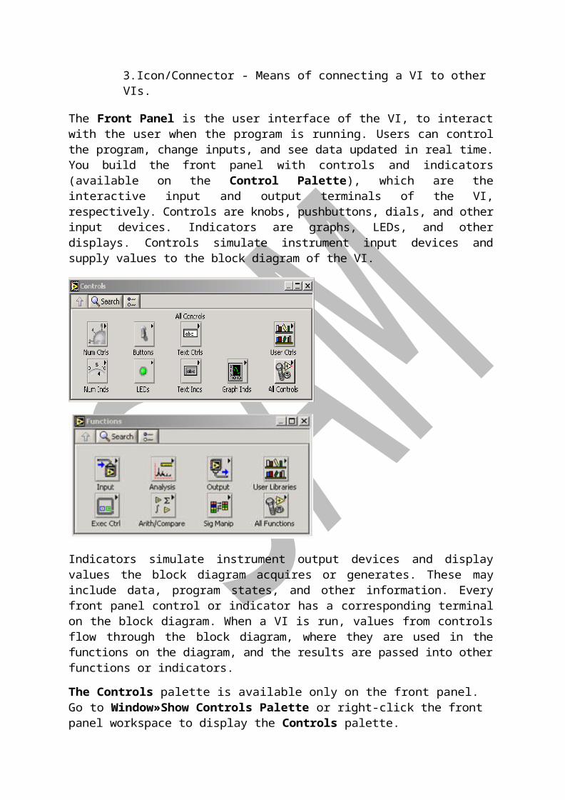
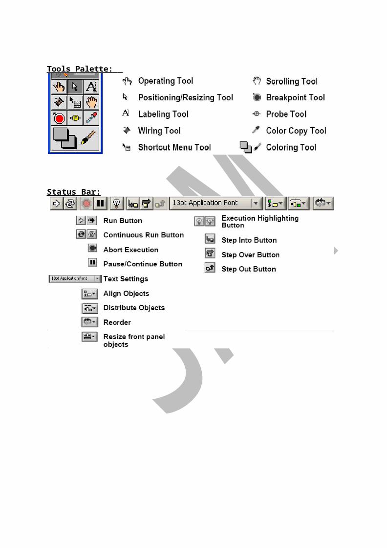
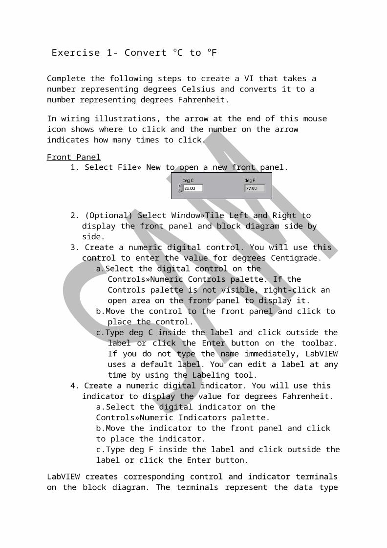
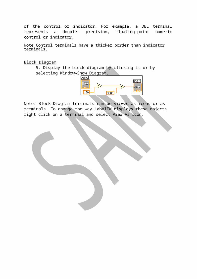
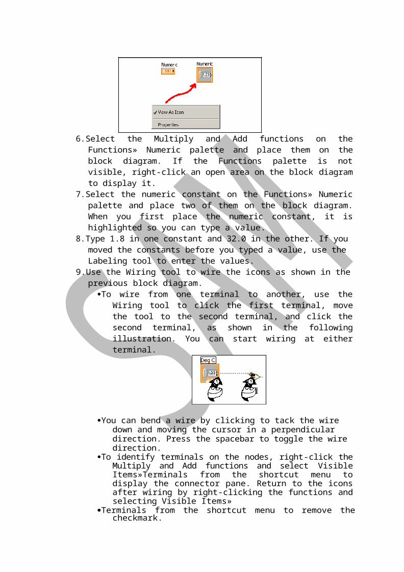
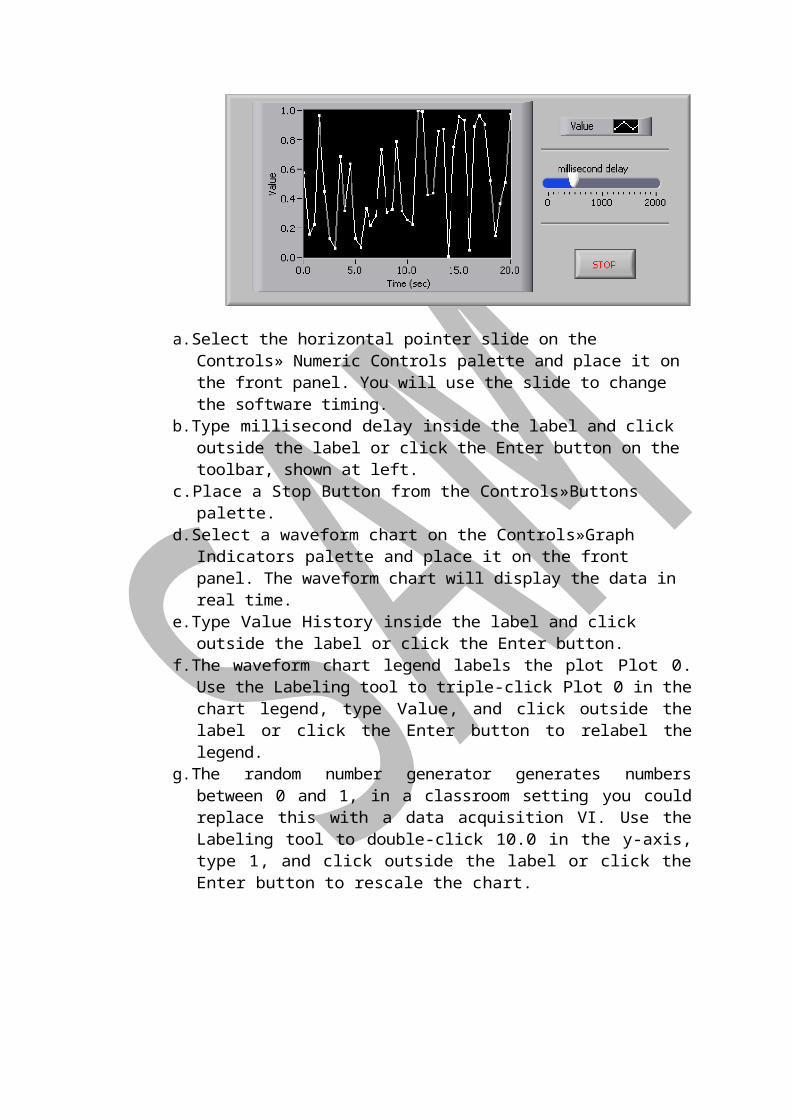
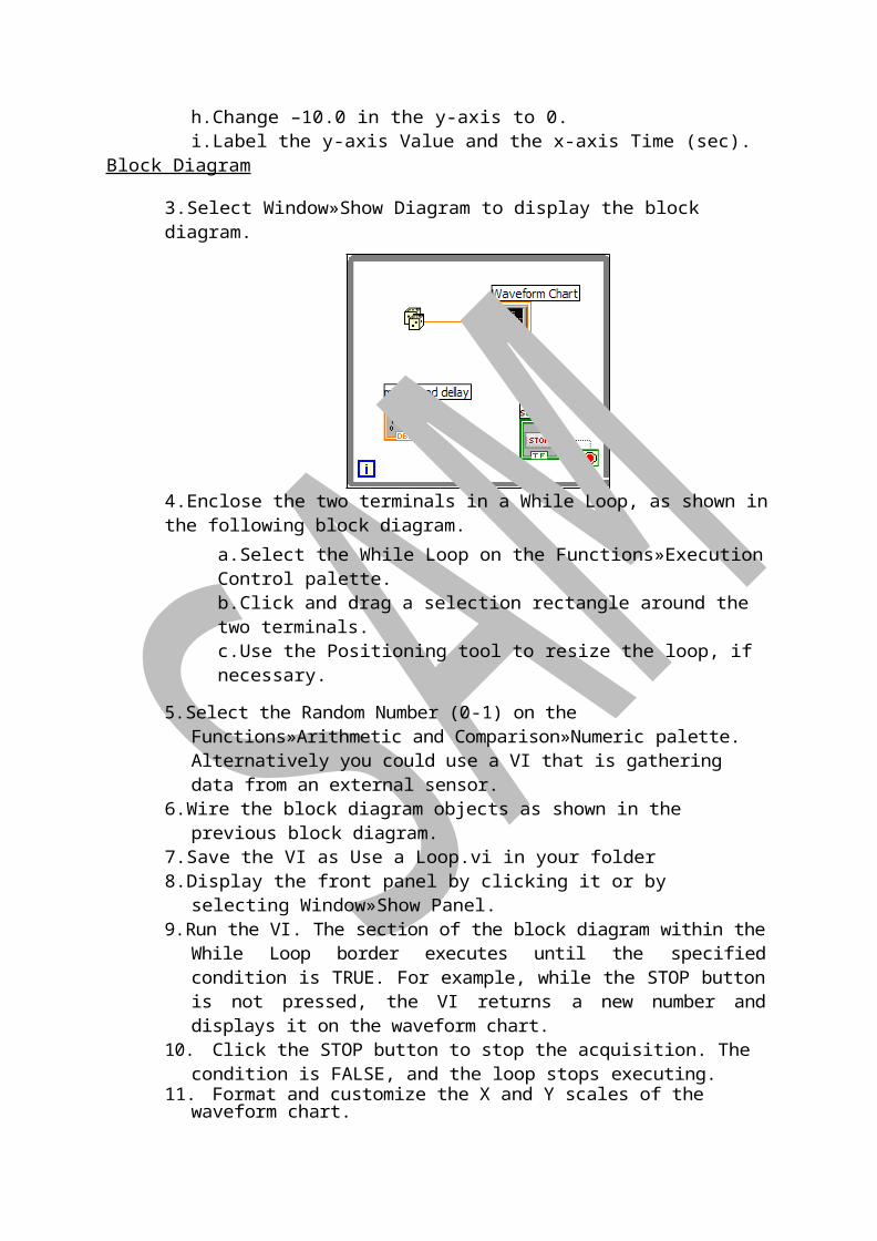
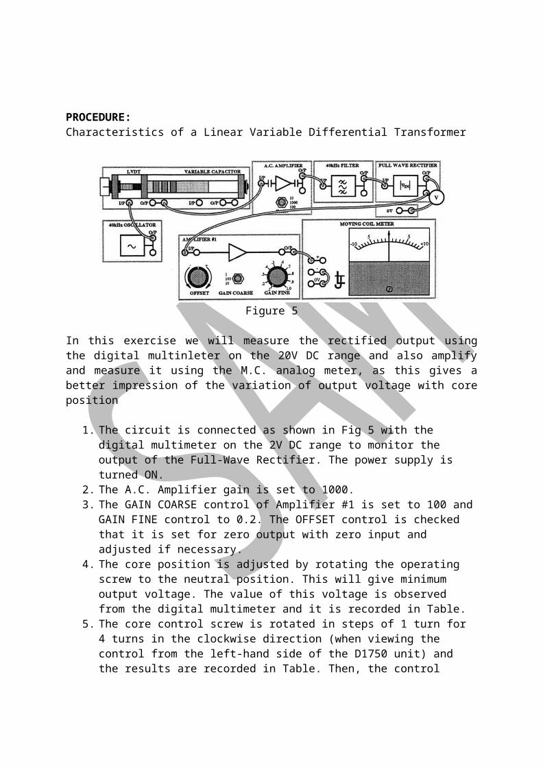
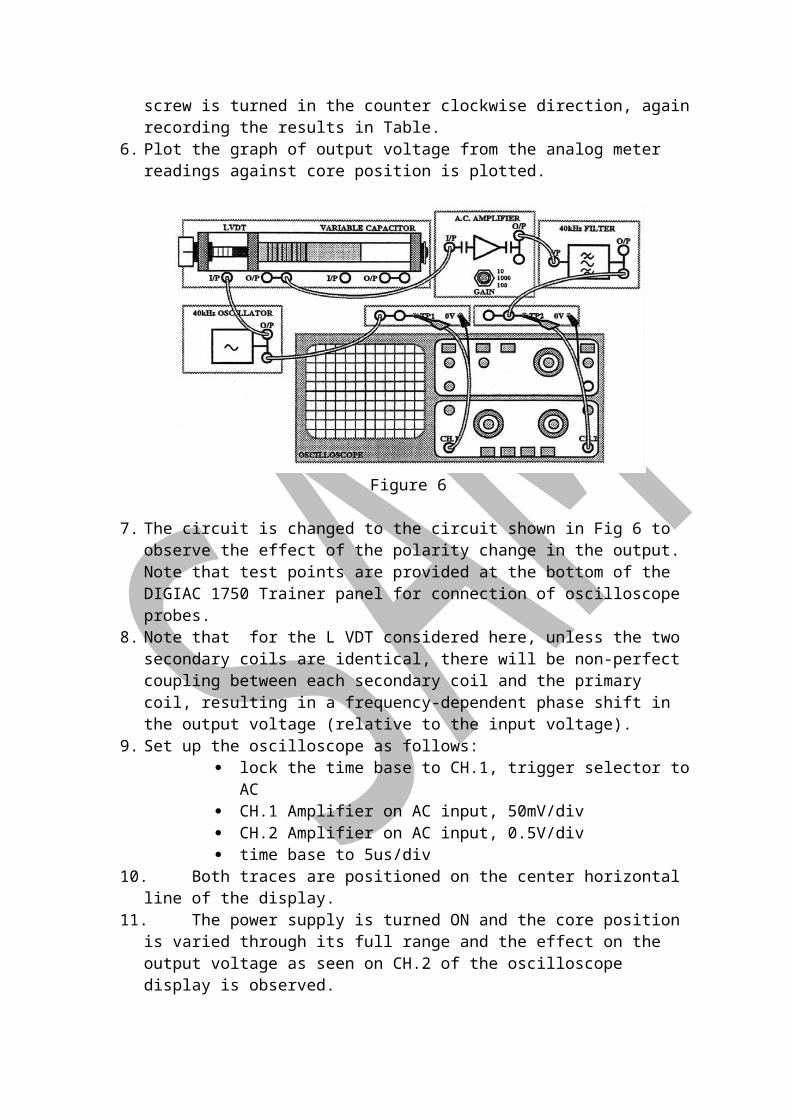