instructions for use · central arctic from the project skijump in 1951 and 1952. subsequent...

Instructions for use

Title Hydrography of the Arctic Ocean with Special Reference to the Beaufort Sea

Author(s) KUSUNOKI, Kou

Citation Contributions from the Institute of Low Temperature Science, A17, 1-75

Issue Date 1962-12-20

Doc URL http://hdl.handle.net/2115/20226

Type bulletin (article)

File Information A17_p1-75.pdf

Hokkaido University Collection of Scholarly and Academic Papers : HUSCAP

https://eprints.lib.hokudai.ac.jp/dspace/about.en.jsp

Hydrography of the Arctic Ocean

with Special ReFerence to the BeauFort Sea-X-

by

Kou KUSUNOKI

Oceanographic Section, The Institute of Low Temperature Science

Received August 1962

Contents

L Introduction _ _ _ _ _ _ . . . . . . . . . . . . . . . . .. 1

II. General background of the oceanographical studies in the Arctic Ocean 2

III; General account of the ice islands . . . . . . . . . . . . . . . . .. 7

IV. Instrumental and observational aspects of the work at Ice Island T-3 in

1959-1960 . . . . . . . . . . . . 10

V. Distribution of temperature . . . . . 13

VL Distribution of chlorinity and density 32

VII. Distribution of chemical elements 38

VIIL Water masses in the Arctic Ocean. 49 IX. Circulation in the Arctic Ocean 63

X. Conclusions 70

Acknowledgments. 73

References . . 73

I. Introduction

This paper is intended to provide a knowledge of the Arctic oceanography,

particularly of the northern portion of the American continent where the oceanographic

data are still extremely sparse, especially winter observations. Actually the Arctic

Ocean held a number of unsolved problems when H. U. SVERDRUP (1950) prepared

his review of physical oceanography in 1950. He emphasized the poverty of infor

mation concerning the character of waters which had been studied only on the Siberian·

European side of the Arctic Ocean. Since the late 1940's oceanographic observations

in the Arctic Ocean have become very active with the aid of aircraft landed on the

Arctic pack ice. The shipboard observations were inevitably constrained within the

coastal waters.

In former days oceanographic observations in the central part of the Arctic Ocean

were made from icebound ships, some of which were caught in the ice with deliber-

* Contriubtion No. 628 from the Institute of Low Temperature Science.

2 K. KUSl'NOKI

ation, such as the drift of the E'ram in 1893-1896. Since World War II a number

of expeditions with the aid of aircraft have been sent to the central part of the Arctic

Ocean to work in parallel with the shipboard observations at the coastal waters. Drift

stations on the ice floes which have served as oceanographic research vessels have

been e:,tablished in the central Arctic. Putting aside the activities of these stations in the early part of 1950's, the situation during the International Geophysical Year will

be worthy of note. Four drift stations on ice were in operation during the IGY,

of which two were on the Arctic pack ice and two were on the "ice island" with

greater thickness than the pack ice. The Soviet maintained two stations (designated

SP-6 and SP~7)'); while the United States established Drift Station Bravo on "Ice Island

T-3."

The present writer spent two periods on Ice Island 1'-3 during 1959 and 1960

and carried out oceanographic observations in the Beaufort Sea. The 1'-3 drifted

from 72SN, 1300 W to 7l.9°N, 160.3°W between May 1959 and January 1961. A total

of 35 oceanographic stations for subsurface observations were occupied during this

period, and 183 bathythermographic observations were made. Taking the drift speed

of T -3 into consideration, the subsurface observations were initially planned to be

made at about two weeks' intervals. Unfortunately several winch breakdown precluded

adherence to this schedule, and a final breakdown of cabJe drum occurred while occu

pying Station 10 on September 1959. A replacement winch was put into operation

on November 19, 1959 and Sation 11 was obtained.

On the basis of the results of obs~rvations made at T -3 the oceanographic features

of the northern waters of the American Continent will be discussed. It is regrettable

that the available oceanographic data in the central Arctic are very few, despite the

fact that the Soviet has sent many parties to the central Arctic. At the time of the

preparation of this paper the available Russian data were those from the SP·-2 in

1950-1951 and others which have appeared in the Russian' literature.

II. General Background of the Oceanographical

Studies in the Arctic Ocean

The Arctic ocean has an area of about 14 x 106 km2 which i3 approximately the size of the United States. From the viewpoint of oceanography the term "Arctic

Basin" which is bounded by the continental slope is frequently used. In a broad

sense the Arctic Ocean is the area surrounded by the Eurasian Continent, American

Continent, and Greenland. The most part of the Arctic Ocean is covered with pack

ice and even in the marginal seas, such as Barents, Kara, Laptev, East Siberia, Chukchi,

and Beaufort, sea ice develops in the winter season. The ice concentration of the central Arctic is not less than 8/10 or 9/10 in summer and it attains nearly 10/10 in winter. The Arctic pack ice is consisted of winter ice and perennial ice. The thickness

of the ice varies from 2 to 4 meters, in some places where the ice is rafted and hum-

,. Abbreviated from "Severnyy Polyus" (North Pole). SP-6 was on an ice island.

Hydrography of the Arctic Ocean 3

mocked the thickness attains to about 30 meters. The Arctic Ocean covered with the

vast ice field plays an important role in the heat budget of the planet earth. Not

only from the viewpoint of the heat budget, but for the water and vapor balance study

of the Arctic Ocean is badly needed. It is weli known that the drifting stations in

the Arctic Ocean were established to attack these problems as a part of the program

of the IGY.

The Arctic Ocean is sometimes compared with the Atlantic Mediterranean because

its main outlet to the North Atlantic Ocean is the area oetween Greenland and Svalbard

(Spitzbergen). The Greenland Sea is the uniqe place where the major water-mass

transfer takes place between the Arctic and the Atlantic ocean. Studies i~ the Bering

Sea, Bering Strait, and the Chukchi Sea have ind~cated that the water exchange through

the Bering Strait is considerably less than that through the Greenland Sea. The water

exchange through the channels between the islands in the Canadian Arctic Archipelago

is believed to be very small.

The Arctic Ocean has been considered as an extensive and deep depression with

a depth of more than 4000 meters since the drift of the Fram led by F. NANSEN (1902)

in 1893-1896. The specially designed ship Fram was intentionally allowed to be

caught in the ice to the north of the New Siberian'Islands from where the ship drifted

across a previously unexplored area, finally escaped to the north of Svalbard. Although

NANSEN could not reach the geographic North Pole, a great deal of information

concerning the Arctic Ocean was collected. The discovery of the character of the

wind-driven ocean currents is well know. From the expedition of the Fram the three

main water masses in the Arctic Ocean were identified; the Arctic Surface Water, the

Atlantic Water, and the Arctic Bottom Water.

In 1925-1928 the Norwegian expedition with the Maud was unable to duplicate

the drift of the Fram, being prevented by the adverse ice condition on the Siberian

shelf. But this expedition made an outstanding contribution to the hydrography of

the Siberian shelf waters, the movement of polar pack, tide and currents, and physical

properties of sea ice. In 1931 the submarine Nautilus made a few observations at

the north of Svalbard, even though she failed to penetrate into. the central part of

the Arctic Ocean beneath the pack ice. The Nautilus expedition confirmed the theory

of NANSEN which suggested the intrusion of Atlantic Water with high temperature

and high salinity under the Arctic Surface Water from the Greenland Sea. In these

years, the hypothesis of Harris on the existence of land at the north of Alaska was

denied, because the tidal records obtained by the Maud gave no evidence of the

existence of land. No land but ice only was seen during the flight of the Amundsen

Ellsworth-Nobile airship expedition in 1926.

In 1937-1940 the Russian icebreaker Georgy Sedov drifted roughly parallel to the

path of the Fram. Soundings and oceanographic observations were made. At the

same time a party led by 1. D. Papanin landed on the ice floe near the North Pole

and drifted to the east of Greenland at an average speed of 9.1 km/day between May

4: K. KUSUNOKI

21, 1937 and February 19, 1938. This expedition was recently designated "Severnyy

Polyus.l." Summarizing the soundings taken during these expeditions, it has been

generally accepted that the central part of the Arctic Ocean is an extensive depres

sion. These paths of drift however did not cover the greater part of the Arctic Ocean,

extending betvveen 1500E and 70cW.

In the spring of 1946 several landings on ice floes were made by the Russian

plane N-169, covering several sites in the region so-called "pole of relative inacces

sibility." Occupying each site for several days, scientists made oceanographic observa

tions and other geophysical studies. The bottom topography of the Arctic Ocean

was still not clear in those years.

Since 1948 the Soviet have continued to send out "High-Latitude Airborne Ex

peditions"; they have established drift stations in the central Arctic. Making com

parison of the temperature of deep layers obtained by the Sedov and N-169, the

Russian researchers came to postulate an upheaval of ocean bottom between the

meridians of 1400E and 175°E. The bottom temperatures were - 0.78°C and - 0.38°C

at the stations of Sedov and N-169 respectively. However this conjecture on the

existence of an underwater range was brought to the attention of the present vvriter

by recent Russian literature (TIMOFEYEV 1960). So far as the present writer is aware,

the Russian activities since 1939 were first publicized in 1954. It should be worth

noting that WORTHINGTON (1953) infered the existence of an underwater range in the

central Arctic from the Project Skijump in 1951 and 1952. Subsequent Russian ex

peditions, particularly in post-war years, were rewarded by the discovery of an under

water range (Lomonosov Range) having a length of about 1800 km. The shallowest

depth was 954 meters (GORDIYENKO and LAKTIONOV 1960). The Russian drift stations

are: SP-2 (1950-1951), SP-3 (1954-1955), SP-4 (1954-1957), SP-5 (1955-1957), SP-6

(1956-1959), SP-7 (1957-1959), SP-8 (1959-1962), SP-9 (1960- ), SP-10 (1961- ).

It was reported that the thickness of SP-6 (ice island) was between 3 and 20 meters.

The bottom configuration of the Arctic Ocean revealed greatly by the Russian is

presented in Fig. l.

Fig. 1 shows the huge underwater range which divides the Arctic Ocean into

two depressions; the Nansen Deep in the North Eurasian Basin and the Beaufort Deep in the North Canadian Basin. The Marvin Ridge running in parallel to the'

Lomonosov Range was revealed by the observations on 1'-3 and at Drift Station

Alpha. In the present paper the terms "Atlantic side" for the North Eurassian Basin

and "Pacific side" for the North Canadian Basin will be used.

According to the Russian researchears the maximum depth of 4689 meters was

measured in the Beaufort Basin. The Makarov Depression, with depths of over 4000

meters, exists within the area between the Lomonosov Range and the Mendeleyev Ridge

and the northern spurs of the Marvin Ridge. The Litke Depression lies in the Atlantic

side with a maximum depth of 5449 meters at 82° 24/N and 19° 31/E. During 1955

and 1958 Russian ships sounded the area between Greenland ~nd Svalbard. The ex-

Hydrograj)hy of the Arctic Ocean 5

Fig. 1. Bathymetric chart of the Arctic Ocean.

istence of the continuous Nansen Sill was denied. The Nansen Sill, foremerly believed

to be about 1300-1400 meters deep, is cut through by a deep-water trough (the Lena

Trough) with depths of 3100-3400 meters in the northern part and 3500-3900 meters

in the southern part (LAKTIONOV 1959). However the depth-soundings in the Arctic

Ocean are still few in number, and it is certain that many minor bottom configuration,

such as submerged valleys, canyons, troughs, rises, and sea-mounts, will be discovered

by future observations. As an example of recent activity in this line, it will be noted

that a minimum depth of 1462 m was recorded at 85°03/N, 171 0 OO'W on the Mende- .

leyev Ridge by the soundings taken from Drift Station Alpha.

In contrast to the oceanographic exploration in the Atlantic side, the investigations

in the Pacific side have made slow progress. In 1951 and 1952 oceanographic obser

vations under Project Skijump were made at various points on the Pacific side by the

use of aviation. As mentioned before, analyzing the temperatures in deep layers,

WORTHINGTON (1953) postulated the existence of a ridge with a sill depth of less than

2300 meters. In the mean time SP-2 (1950-1951) drifted in the western part of the

Pacific side alon.g the meridian of about 175°W, between 76°N and 81°N. This station

(abandoned) was found in April 1954 to the north of Wrangel Island (75°04/N, 1720

6 K KUSUNOKI

20/W) and it was conjectured that the SP-2 had drifted ciockwisely in the Pacific

side.

In the post·war years, shipboard observations have been made in the coastal waters

along the American Continent. Some ships thus penetrated into the pack ice as far

as to 75°N and also the observations in the waters of the Canadian Arctic Archipelago

became active in recent years. The following names of the Canadian and American

vessels may be cited: Atka, Burton Island, Cancolin, Cedarwood, Eastwind, Eldo

rado, Labrador, Nereus, and Northwind.

The drifting stations established by the United States provide useful means for

oceanographic research of the Pacific side of the Arctic Ocean. The paths of drift

of ships and stations on ice floes suggest the scheme of the surface circulation of the

Arctic Ocean. The subsurface observations made at those stations and ships reveal

the physical, chemical, biological, and geological features of the Arctic Ocean. In

Fig. 2 the paths of drifts are represented; in it the drift of ice islands in the Pacific

__ ~ ______ ~~~ __ +-______ ~-;O .

30

Fig. 2. Drift paths of ships and ice islands.

side is emphasized. A very larg~ anticyclonic vortex is to be noted from Fig. 2. More

detailed information on the paths of drift stations and icebound ships may be obtained

in many publications; e. g., in the "Oceariographic Atlas of the Polar Seas, Part II, Arctic" (U. S. NAVY HYDROGRAPHIC OFFICE 1958).


III. General Accout of the Ice Islands

On August 14, 1946 an enormous mass of floating ice among the polar pack was

discovered less ·than 300 miles* north of Point Barrow, Alaska by an aircraft of the

U. S. Air Force. This Vias originally recognized by means of the radar in the aircraft,

hence designated "Target X" or "T -1" in later dates. In the succeeding years the

movement of T -1 has been traced by radar and visual observation. The T -1 had an

area of about 600km' and its surface was even with a broad undulation. Many con

jectures have been made as to the thickness, the location of calving, growth mechanism,

surface topography, inner structure and so forth. An extensive search for other ice

islands was commenced in May 1950 and led to the discovery of T -2 and T -3 in the

Pacific side of the Arctic Ocean. Also a number of small islands were found aJ;Ilong

the channels in the Canadian Archipelago. The T -2 with an area of 800 km', the

largest one ever found, was located at 84° 40/N, 16T ODIE on July 19, 1950.

Ice Island T-3 was first sighted at 75°24/N, 173°00/E on July.29, 1950. This

island was later identified as having already been photographed on April 27, 1947 at

79° 50/N, 104° OO/W, 30 miles north of Isachsen Peninsula in Ellef Ringes Island. The

three Ts had an enormously large mass different from the ordinary polar floes and

surface of the islands was surprisingly smooth at the time of discovery. The exami

nation of past publicatio~s led to the opinion that these ice islands were very likely

the so-called "disappeared islands in the Arctic Ocean." (KOENIG et al, 1952, KUSUNOKI

1955 a, 1960 b).

In the meantime, the Russians reported that the existence of ice islands was first

discovered by the pilots of High-Latitude Airborne Expeditions and ice reconnaissance

flights. They designated those islands as the Kotov (discovered in March 1946), the

Mazuruk (1948), and the Perov (1950) after the names of the pilots. So far as the

present writer is aware, the identity between those islands and the three Ts is ambigu

ous. Setting aside the problems of priority of discovery, subsequent observations of

the position of the ice islands have enabled one to estimate the surface circulation in

the Arctic Ocean, particularly of the Pacific side. The clockwise path of drift of T-3

illustrated in Fig. 2 indicates that it has taken about ten years to complete the circular

motion in the Pacific side. The av~rage speed of drift was 0.8 km/day.

The scientific work at T -3 was initiated in April 1952 when a small party led by

J. o. Fletcher made the first landing to establish the scientific station. Thereafter

the island has been occasionally called "Fletcher's Ice Island" or "Fletcher's Ice Island

T-3". The scientific observations at ice islands can be divided into two catagories.

In the first category, observations on meteorology, oceanography, gravity, earth mag

netism, and aeronomy are included. For the sake of these observations the ice island

serves as a convenient means, just like a research ship. The second category includes

". Nautical miles are used in the present paper. 1 n. mile = 1852 m.

8 K. KUSUNOKI

---~----, OLD QCk "-

SILK HILL' HYDRO STATION Ice

18S8 than one meter above seQ lev'l

x o ~OLBY BAY

OLD CAMP

(1952-56) ) .• ~ ~HYD'l.o STATION GRAVEL 00 CAMp·(J960-)

IGY CAMP (J957-591

ICE ISLAND J-3

o 2 4 6 8 10 KM ~I __ ~~I~~~I __ ~~I __ ~~I __ ~-JI

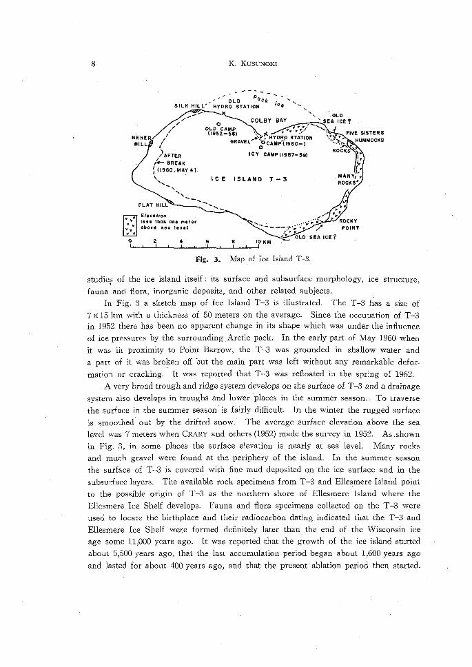
Fig. 3. Map of Ice Island T-3.

studie~ of the ice island itself: its surface and subsurface morphology, ice structure,

fauna and flora, inorganic deposits, and other related subjects.

In Fig. 3 a sketch map of Ice Island T -3 is illustrated. The T -3 has a size of

7 X 15 km with a thickness of 50 meters on the average. Since the occupation of T-3 in 1952 there has been no apparent change in its shape which was under the influence

of ice pressures by the surrounding . Arctic pack. In the early part of May 1960 when

it was in proximity to Point Barrow, the T-3 was grounded in shallow water and

a part of it was broken off but the main part was left without any remarkable defor

mation or cracking. It was reported that T -3 was refloated in the spring of 1962.

A very broad trough and ridge system develops on the surface of T -3 and a drainage

system also develops in troughs and lower places in the summer season. To traverse

the surface in the summer season is fairly difficult. In the winter the rugged surface

is smoothed out by the drifted snow. The average surface elevation .above the sea

level was 7 meters when CRARY and others (1952) made the survey in 1952. Asshown

in Fig. 3, in some places the surface elevation is nearly at sea level. Many rocks

and much gravel were found at the periphery of the island. In the summer season

the surface of T -3 is covered with fine mud deposited on the ice surface and in the

subsurface layers. The available rock specimens from T -3 and Ellesmere Island point

to the possible origin of T -3 as the northern shore of Ellesmere Island where the

Ellesmere Ice Shelf develops. Fauna and flora specimens collected on the T -3 were

used to locate the birthplace and their radiocarbon dating indicated that the T -3 and

Ellesmere Ice Shelf were formed definitely later than the end of the Wisconsin ice

age some 11,000 years ago. It was reported that the growth of the ice island started

about 5,500 years ago, that the last accumulation period began about 1,600 years ago

and lasted for about 400 years ago, and that the present ablation period then started.


The date of calving of T -3 from Ellesmere area was estimated by examining the plant

specimens and mosses found on both T-3 and Ellesmere. It was deduced that the

T -3 left from the shore of Ellesmere Island at a time not earlier than 1935. These

conjectures are based upon the observations at T -3 during 1952 and 1955. and upon

surveys at the northern shore of Ellesmere Island, in paralell with laboratory studies.

During these years the station at T -3 was evacuated in May 1954 when the island

drifted into the proximity of the land weather stations of the Canadian Arctic. A

party re-occupied T-3 during the period April to September in 1955. CRARY (1956,

1958, 1960) sumarized his studies on T -3 and Ellesmere region.

Prior to the period of the IGY the oceanographic observations on T-3 had been

carried out at the "Old Hydro·Station" near the "Old Camp". An ice-hole opened

in the perennial sea ice attached to the T -3 was used for the oceanographic work.

In Colby Bay area, between Silk Hill and Five Sisters Hummocks, many-wintered polar

ice with a thickness of about 5 meters existed. Between 1952 and 1955 eleven stations

were taken, ten in 1952-1953 and one in 1955. Biological investigations and bottom

sampling were made at Old Hydro-Station. Details of the facilities of this station

were described by MOHR (1959). The data of temperature and salinity during this

period were presented by WORTHINGTON (1959). However, salinity values for Sts. 1-4

are not given because of the difficulty in shipping of water samples under severe Arctic

environment and long transportation route.

As already mentioned, the United States established two drift stations for executing

the IGY program in the Pacific side of the Arctic Ocean. The station Alpha on the

ice floe was maintained between the early spring of 1957 and December 1958 when

the station was evacuated due to the ice-breakup. The second one on the pack ice,

designated Charlie, was set up at about 300 miles north of Point Barrow. This station

was active from June 1959 to January 1960 when inevitably evacuated because of ice

breakup. The icebreaker Burton Island was successful in establishing the third one,

Arlis-1 *, on the pack ice in the Beaufort Sea on September 12, 1960, and this station

was abandoned in the late of March 1961. A new ice island bearing rocks that are

hea.ped about 15 meters high in places was found in late may, 1961 (Arlis-2). The

new ice island was roughly 150 miles north and slightly east of point Barrow at the

time of discovery. It was reported that the new ice island is fifty feet thick, two

miles wide and three miles long.

Ice Island T -3 (designated Drift Station Bravo in the IGY) drifted from 82° 51'N,

96° lO/W on May 20, 1957 (oceanographic station No. 12) to 80° 02/N, 115° 50/W on

May 15, 1958 (station No. 17) during the IGY. -Those oceanographic stations were

numbered in a series of observations dating back to 1952. The results of observations

were presented by FARLOW III (1958) and APOLLONIO (1958) who did the biological

work. Between May 26, 1958 and September 28, 1958 a total of 21 stations were

* Arctic Research· Laboratory Ice Station (Arlis).

10 K KUSUNOKI

taken by COLLIN (1958), a representative from the Canadian Fisheries Research Board.

The oceanographic work in 1959-1960 has largely in the nature of continuation

from the program in the IGY. During this. period a new hydro-station was established

on the perennial sea ice in Colby Bay (see Fig. 3). During the summer of 1959 the

present writer with the assistance of J. Muguruma, who conducted the later winter

observations, carried out the observations. The preliminary results have been reported

by KUSUNOKI (1960 a) and MUGURUMA (1961) for summer and winter observations

respectively. In the early part of May 1961 the T -3 grounded at about 72°N, 1600 W

and has remained in approximately the same position until the spring of 1962. The

observations between May and September 1960 were made by Mugurumu and K.

Higuchi. A summarized report on the observations during 1959-1960 is pr2~entd

by KUSUNOKI et al. (1962).

It is to be noted that many reports on the results of observations accomplished

at T-3 during the period of 1952-1955 under various scientific disciplines are presently

in course of publication (BUSHNELL 1959).

IV. Instrumental and Observational Aspects of the Work

at Ice Island T-3 in 1959-1960

In May of 1959 a new hydro-station was established on the old pack ice in Colby

Bay and a laboratory in the main camp was equipped. At this itme the pack ice with

a width of 1 to 2 miles had been attached to the island for at least several years.

An ice-hole with a diameter of about 2 meters was opened through the pack ice of

5.5 meters thick with the aid of explosives'. In the vicinity of the hydro-station there

were erected two shelters for seismic work and underwater acoustics. The location

of the hydro-station was selected on a flat-topped broad ice mound in the uneven old

sea ice.

A two-section J amesway shelter was constructed beside the ice-hole to provide

a place for storing provisions and working space. A gasoline engine driven winch

was set up between the Jamesway shelter and the ice-hole. An A-frame equipped

with a meter wheel was set on timbers arranged in parallel crosses over the ice-hole.

During the summer of 1959 troubles in the winch were experienced and on September

9 the cable drum was broken during the occupation of St. 10. A new winch was

supplied on October 29 and this was installed within the shelter which had been

moved onto the lower ice surface of the frozen melt water pool around the ice-hole.

The transfer of the Jamesway shelter onto the lower ice surface was necessitated by

the heavy ice ablation during the summer.

Until the early part of June the air temperatures were usually below O°C; so that

an ice rind having a thickness of about 3 cm formed on the surface of water in the

ice-hole in every day. Between June to September, the ablation of ice, both on the

island and the sea ice, took place intensively. The average ablation loss over the island

was estimated as 160 cm in ice thickness. Even on the surface of pack ice with high


albedo the ablation was very active. The explosive dust around the ice-hole accelerated

the melting of ice there.

Owing to the sub-zero temperatures III the middle layer of pack ice an accretion

of ice took place on the wall-surface of the ice-hole. The diameter of the hole de

creased to about 30 cm from May 28 to July 2. The accreted ice was dynamited,

but this was not effective, and finally the melt water having a temperature of slightly

above O°C· was channeled into the ice-hole. This water melted the newly-formed ice

and the shape of ice-hole in the final stage was truncated cone. This shape was very

favorable for the oceanographic cast when the cable was inclined by currents. The

thickness of fresh water filled in the ice-hole was less than 6 meters even in the period

of maximum discharge.

In the middle of August the formation of anchor ice in the ice-hole was frequently

observed. It was believed that the anchor ice was formed at the interface between

the warm fresh water arid underlying saline water with low temperatures of nearly

freezing point. A great amount of anchor ice was scooped out almost every day.

The ice ablation ceased in the early part of September; the discharges from the streams

on T -3 decreased and the melt water pools 011 the pack ice qegan to solid.

During the ablation season a heavy tent sheet was spread over the ice-hole to cut

off the intensive solar radiation. The parachute cloths used for air-drop were skirted

around the Jamesway shelter. However, at the end of the season, an ice rampart

about 2 meters high remained in' the shaded area around the ice-hole and the shelter

was left on an ice mound of barely 2 meters height. The ablation was very pronounced

at the main camp area which was much contaminated because of oil and dust particles.

This necessitated the transfer of the main camp to a new site in the spring of 1960

(see Fig. 3).

In the winter of 1959-1960 the ice-hole was thermally insulated by a wooden frame

and. heavy cloths. The ice rampart which remained around the ice-hole was useful

III the construction of a covered frame. An oil stove set inside the hut was enough

to keep open the ice-hole even at a low temperature of -40°C. During this period

the diameter of the hole was kept about one meter. Due to the damage to the cable,

some of the casts were restricted to approximately 1,000 meters depths.

On May 4, 1960 the T -3 ran aground at the position of 710 53/N, 1590 37/W and

has remained in approximately the same position (71 0 52/N, 1600 20'W) until 1962, with

the exception of drifts which occurred in the middle of May and J lily 1960. As the

shelter had been set up on a low elevation, flooding on the ice floor around the hole

took place in the middle of May. At a site about 15 meters from the edge of the

island a new ice-hole was opened at the end of May. The new ice-hole; one meter

square, was opened with chain-saw and explosives through the ice with a thickness

of 5.2 meters. On this occasion, a four-section Jamesway shelter equipped with a wineh

was placed on heavy wooden skids and pulled over the hole. One floor panel was

removed for the cast. In the middle of July, heavy ablation occurred around the

12 K. KUSUNOKI

shelter, but a small hand winch sufficed for carrying on the observation, rather than

operating the heavy gasoline-driven winch inside the shelter set on the ice mound. At

the end of August, soon after the third grounding of the island, the program was

suspended due to the breakup of the pack ice in Colby Bay and the shelter was

removed onto the island. Fortunately the pack ice around the ice-hole was not broken

off, so that the observation was made by IIleans of the hand winch through the un

covered ice-hole.

In 1959 electric power was supplied from an electric generator driven by a gasoline

engine which was set up near the shelter. In the spring of 1960 the main camp was

moved to a new site and electric transmission lines were Instailed to the shelters in

Colby Bay area.

A description will be given on the instruments and the method of chemical

analysis.

Water sampling bottles: Six Nansen type water sampling bottles each equipped

with a two-thermometer frame were used at each cast. Additional Nansen bottles

were found at the main camP, but due to the limitation of thermometers, only six

were lowered at each cast. Bottles with protected-unprotected pairs of thermometers

were placed between bottles with two-protected thermometers at each lowering. This

was a necessary procedure to determine the depth of the observation layers.

Re·versing thermometers: All protecte~ thermometers were graded for low temper

ature range, viz., -2 to 8°C or -2 to 10°C. The values of the pressure coefficients

of unprotected thermometers were calibrated at depths of 500, 1000, 1500, and 2000

meters when there was no perceptible inclination of sounding wire. A calibration of

the meter wheel was also· carried out by paying out .the wire less than 20 meters.

A conversion factor of 0.982 was fina,lly adopted for readings of the meter wheel. On

several occasions a separation of the mercury in the capillaries of the reversing ther

mometers resulted when the thermometers were lowered into the cold water.

Bathythermograph (BT): A bathythermograph was used for the observation of

temperature down to about 250 meters. At each cast of the BT the temperature at

15 meters, on occasionally at 0, 10, or 15.5 meters, was read by means of reversing

thermometers attached to the Nansen bottle. The surface temperatures exhibited

a wide variation under the influence of summer air temperatures, solar radiation, and

the local effect of the ice hole. For this reason, the temperature at 15 meters was

read to correct the BT records. The BT casts were usually made on alternate days,

and at the beginning and end of each subsurface serial observation. Malfunctioning

was experienced during the winter of 1959-1960. The results of BT observations

were presented in the appendix of the report of KUSUNOKI et al. (1962).

Water preserving bottles: Ordinary glass bottles with rubber stoppers were used

for the samples for chlorinity titration. During the summer of 1959 a sufficicent

number of glass bottles for complete oxygen analysis was not available; therefore,


sampling depths were predetermined to cover the standard depths only. Polyethylene

bottles, 150 ml in content, were used for silicate-Si samples. Since the analysis' was

performed at the chemical laboratory at T-3, problems such as freezing 'of water,

evaporation, or breaking of bottles, frequently experienced in previous years during

shipment, were eliminated.

Method of chemical analysis

Chlorinity: Knudsen's method modified by the use of uranm as an indicator

(Fajans-Miyake's method) was adopted. All the samples, with the exception of brackish

surface waters, were titrated independently by the persons until the results were in

agreement with an error less than 0.019(,c. In the winter of 1959-1960 titrations were

performed by one person three or more times, if necessary, to achieve the required

precision.' The normality of AgN03 solution was determined by the use of "Eau de

mer normale" prepared by the Hydrographical Laboratory in Copenhagen. Fresh and

brackish water less than 17% in chlorinity was titrated by Mohr's method.

Dissolved oxygen content: Dissolved oxygen content was measured by Winkler's

method using KIO, as the standard. The saturation percentage was calculated by

the use of Fox's formula. Since the content of the oxygen bottle was 250 ml, two

or more titrations were possible and results were averaged.

Silicate-Si content: The content of silicate-Si was colorimetrically determined by

the method of Dienert and W anden bulke. A Klett-Sommerson colorimeter was

used for this procedure. The analyses were performed within a few hours after

sampling, in order that the concentration of Si might not undergo any appreciable

change due to biological activity. Since the water temperatures of the Arctic Ocean

are very low, errors due to the preservation of sampled waters may be very small.

The data of the subsurface observations have been interpolated to provide standard

depths and presented in the appendix of the report of KUSUNOKI et al. (1962).

V. Distribution of Temperature

The distribution of temperature in the Arctic Ocean depends upon a number of

factors, foremost among which are the amount of radiation income, the ocean currents,

and the ice condition. , The intensive solar radiation in the summer, almost 24 hours

of daytime, accelerate the melting of pack ice and warm up the surface water. The

temperature of the surface water, particularly of the open waters, sometimes exceeds

GOC. At this time, the river discharges from the Eurasian and North American con

tinents contribute to dilute the surface salinity and to increase the temperature. It is

known that the warm Atlantic Water ~nters into the Arctic Basin beneath the cold

surface water. The inflow of Pacific water through the Bering Strait exerts a sub

sidiary effect upon the temperature distribution of the Arctic Ocean, particulary of

the Beaufort and Chukchi Seas. The sea ice in the Arctic' Ocean plays an important

role in the vertical and horizontal distribution of water temperature. In general, very

14

131°W 136°

_72°N

K. KUSUNOKI

ICE ISLAND T-3

JUNE - SEPTEMBER 19159

o OCEANOGRAPHIC STATION

• BT STATION

G:0 SIZE OF T·3

135° 134° 133° 1320

Fig. 4 a. Path of Ice Island T -3 and posltlOns of stations, June-September 1959.

ICE ISLAND T-3 SEPTENBER- NOVEMBER 1959

0 OCEANOGRAPHIC STATION

• 3T STATION ,.L X.i 5

~ \ X-21

131°

11.5°H

130·

71°M

72°N

ST.IO

(~ V V ST. II

U L.--f.31

IX-28 ~ 71° r---

144°W

Fig. 4 h.

XI-11

I 142° 1400 13Bo

Path of Ice Island T -3 and positions of stations, Septemb~r-November 1959.

71·

1360

Hydrogr'aphy of the Arctic Ocean

ICE ISLAND T- 3

NOVEMBER 1959 - FEBRUARY 1960


• BT STATION

ST.12

15

... ~~=:::::::::_'""' ST. II 3~

• XIi-21 XH9

150 0 W

Fig. 4 c. Path of Ice Island '1'-3 and positions of stations, November 1959·February 1960.

ICE ISLAND T-3

MAR C H - 0 E C E M B E R 1960


• B T STATION

BEAUFORT

POINT BARROW

SEA

Fig. 4 d. Path of Ice Island T -3 and positions of stations, February-December 1960.

72°"

11-10

16 K. KUSUNOKI .

stable stratification IS observed at the top layer in the summer and this stratification

is eliminated by the winter vertical convection due to the formation of ice.

In order to discuss the distribution of temperature in the Arctic Ocean, particularly

of the Pacific side, the data taken at T -3 during 1959-1960 will be analyzed.

The oceanographic observation stations occupied at T -3 cover the area of the

southern Beaufort Sea between 70.S-72.5°N and 130-160.3°W. The locations of the

oceanographic and BT stations are illustrated in Fig. 4 a, b, c, and d. These figures also

indicate the path of the drift between June 1959 and September 1960. As mentioned

before, the T-3 remained at 71° 52/N, 1600 20'W between July 29,1960 and the spring

of 1962. Before the grounding IS stations were occupied during the westward drift

in the southern Beaufort Sea. In the vicinity of the grounded position, Stations 19

through 35 were occupied.

In order to exhibit the general information concerning the vertical distribution

of temperature, plots of the temperature data form all stations taken at T -3 are given

in Fig. 5, in which the data from Sts. 19 to 35 on the shallow shelf are shown in

open circles.

With the exception of the summer values at the surface, the temperatures at the

surface Jayers of less than 50 meters were very low. In some cases, especially at

Sts. 19 to 35, the supercooling of water to the extents of 0.05°e was observed in the

upper layer. Similar phenomena have been observed at the estuaries on the Okhotsk

sea coast of Hokkaido and a quantitative discussion on the occurrence of supercooling

was given by FUKUTOMI et al. (1950).

A minor maximum, more pronounced in winter stations, was observed at each

station at an average depth of 75 meters. The maximum value of -l.OSoe was

observed at St. 17 taken on February 22, 1960 at about 72°N, 153°W. The second

minimum of -l.46°C in average at 150 meters was recorded. A very remarkable

thermocline existed throughout all stations between 200 and 300 meters. Below this

level the Atlantic Water, having positive temperatures, was always found. The 'average

upper and lower Ooe-isotherms were at 2S0 and S50 meters. The average maximum

temperature of the core of the Atlantic Water was 0.42°e at 450 meters. At depths

below 900 meters the temperature decreased gradually and a temperature of -0.43°e

was recorded at about 2000 meters. Due to the limitation of the cable the present

observations did not cover the temperature profile down to the bottom at deep stations.

However the data from other sources, e. g., Project Skijump, SP-2 and the T -3 in

previous years, indicate that the increase in temperature toward the bottom is at a rate

of adiabatic heating. It seemed that the average minimum temperature of -0.43°e

occurred at a level slightly below 2000 meters in the deep layer.

The vertical distribution of temperature at each station will be recognized from

Figs. 6 a, b, c, d and e, in which the results of observations on chlorinity, oxygen

content, silicate-Si and computed density in sigma-t are included.


T E M PER A T U R E, ·C -I 0 -2

o ~oho eo ~...J.g.....Jo-• ...1.0-"/, ..... .s>iatPI~--l-.'" -L I

o • ••••••

(J)

0::: bJ

IbJ

200

400

,; 600

z

J: Ia... bJ 800 c·

1000

1500

2000

f-

f-

. r--

-

... •• _ .. ---.. .... •.. -... - ., ... -... •• • ....

• . -~ ~

•• • STATIONS 1-18 ...

l-0 STATIONS 19-35 ...

to-• ~ . ••

.f' . ~ •

. '" ... " .. • .. ..

• I

I .IA I I

Fig. 5. Vertical distribution of temperatures observed at T-3 in 1959-1960_

17

-

Fig. 6 a represents the vertical distribution of temperature in the middle of ~ummer,

June 30, 1959. The heating of the surface layer is clearly notable. It should also

be pointed out that a minor maximum in temperature was recognized at about 100

meters. As stated previously, this minor maximum was prominently observed at 75

meters depth of St. 17 (Fig. 6 c), while less pronounced at St. 11 (Fig. 6 b). The

temperature in the deeper layers below thermocline at about 200 meters did not show

great change from one locality to another. Figs. 6 d and 6 e are shown as examples

of the vertical distribution of temperature and other oceanographical elements in

shallow water on the shelf.. The former was occupied in the middle of May when

. the winter vertical convection reached down to the bottom. A very homogeneous

18 K. KUSUNOKI

25 26 27 28 O"t.

0

200

400

600

800

1000

1500

2000

0

0 2

16

("

a: .... I-.... 2

z

::J:

I-0.. .... Q

10

4 6

17

-I

I I I , , ? 1 , 1 1 1

6 1 , , , , , o 1 1 I I I 102 I 1 I 1 1 o , , I I I I , I o , I I

20

8 10

18

0 L

JlO all

mL/l

- ,

•

DEPTH

Si

O2

19%. CL ( ( 8

I ·c T

JUNE 30.1959

ST.5 71 0 58'N

132 0 21'W

I

6 \ \

" , I

o I I

6 I I I I I o , , I I I

O"t 0 I I I I

b I I I I I I I I o I , o I I

cr.

1480m <j>

/ ///////J////////////// // // /////,/

L-__ ~ __ ~'~~~ __ ~I ____ ~ __ ~I~ __ ~ __ ~I __ ~~ __ ~ __ -L __ ~I S 29 30 31 32 33 34 35%0

Fig. 6 a. Vertical distribution of temperature, density, and chemical elements at Station 5, June 30, 1959.

25 I 0 I 16 I

-2 0

200

400

600

800

1000

1500

29


26 27 28 at I I I 2 4 (3 8 10 mL/L °2 I

17 18 19 °1 .... CL I I I

-I 0 ·C T I

NOVEMBER 19, 1959

z

l: ... Q.

.... co

30

---- ...... 0....... ,,0"- ST. II ........... <.'

" - .... Q... ........

. 09'N OO'W ? ..... 0 ............

• -_ ............ --' .... 0 , '~ , .... " b ~ , , I \ o 0 I ' I ' I b I ' I '

? \ I I

0 I I

~ , b 0 I I I I I I I I I

I , I I ,

0 , I I I

O2 b T <Tt, I 0 I

31

'0 I , o I I ,

o , I I I o 1 I I

DEPTH 2378 m

I 32 33 34

I I I , 0 I I I I I 1 I

~ , 0 \ I I 6

I

0 I, 1 6 I I

Fig. 6 h. Vertical distribution of temperature, density, and chemical elements at Station 11, November 19, 1959.

CL

S

35 °/00

20

25

0 1

0 1

16 I

-2 0

200

400

600

800

1000

1500

2000

2 1

r-b ...

........ _---

fI)

II: UI ~

UI

~

Z

x: ~ Q.

UI Q

Si

DEPTH 1890m

4 I

26

10 I

17 1

-I

6 I

K. KUSUNOKI

8 I

27

20 , 10 ,

18 I

0

28 crt

..J JI 9 tilL Sl

m~L °2 ip 0/00 CL

I

°c T

FEBRUARY 22. 1960 ST.17

b

O2

• , o , , ? I'

? , o I I I , I

? I 1 I

6 I

I I I I I I 1 I , I ,

.0 I , I , , o I I , ,

6 I I I ,

T (it

6 I I 0 , I ,

0 I , , , , • 0 , I I , I

6 I I ! I , I I , I I

b I I

6 I , I I I

6 I I I ,

1 '1 I

I - • °

CL

o • I

/77)77777777/77/777777777777777

~I~ __ ~ __ ~I~ __ ~ __ ~I ____ -L __ -LI ____ L-__ -LI __ ~ ____ ~I ____ ~ __ ~I S 29 30 31 32 33 34 35 °ko

Fig. 6 c. Vertical distribution of temperature, d~nsity, and chemical elements at Station 17, February 22, 1960.

Hydrography OJ the Arctic Ocean 21

24 25 26 CTt ! I I

0 10 20 30 51 I I I I

0 2 4 6 8 1,0 mlyL O2 }'g aiL

! I I I

16 17 18 I~%. CI I I I

-2 -I 0 ·C T 0 I b

I I , , , 0 J J

I I

J

J i I

• J

10 6 6 T 51 : O2

CL ( CTt , I , , I I J I I ,

0 I J I <II MAY 16, 1960 I a: I

5 T. 20 I W

20 0 I-71· 51' N I !oJ

I 159· 40'W I :lE

I I Z I 0 I I :I: I l-I a. I I !oJ

30 0 0 I I ! I I I 0 \ \ \ \ I ,

40 \ \ I , \ , \

I \ OEPTH 0

\ 0

lI2 m I I. \

I \

Fig. 6 d. Vertical distribution of temperature, density, and chemical

elements at Station 20, May 16, 1960.

22 K. KUSUNOKI

~ ____ ~ ______ ~ _____ 2~~ ______ ~ _______ 2L~ __ ~ __ ~ ____ ~2r ~t 24 , 0 10 , ,

9 ~ 4 , ~ ___ ~ ____ -'---___ """' ____ ----.J' ____ --,I,o ml/L O2

15 16 11 I I ,

3p JlQo/L

18 0/00

I

Si

40 I

CL 19 I

-2 -I o T

10

20

30

, , '0

I I

6 , \ \ \ \ \

\ '0 , ,

\ \

\ \ ,

'0 .... ...

p 4 I , o I I I I I I I

b I I I I I , I

DEPTH 38.5 m

SEPTEMBER 5, 1960 ST. 35

11 0 51.1' N

160· 20' W

tf)

II: .... .... .... :IE

z

:J: .... II. .... Q

77777777777777777777777777777777777777

Fig. 6 e. Vertical distribution of temperature, density, and chemical

elements at Station 35, September 5, 1960.


-1.0 ...-----~-----------

ru -1.5

~

III a: ::> 10 20 3.0 10 20 l-e( JUNE 1959 dULY n: III Q. :IE III l-

n: ~ -1.0 e(

~

10m

-1.5 10 20 30 10

JULY AUGUST 1959 SEPTEMBER

-1.3

<.> . -1.5 ...... 10m Z 10m

III a: :::> 20 30 10 20 30 10 I-

"' iii: NOVEMBER 19 Ii 9 DECEMBER JANUARY 1960 ... Q. :II III ... iii:

·-~·.3

III l-e(

~

,. I , 20 50 10 20

JANUARY 1960 FE B RUARY !\tARe"

Fig. 7 a. Annual variation of temperature (at 15 meters except where

noted otherwise). June 1959-September 1960.

24

-I. 5

!: -1.7

... ~ le '" ... .. : -1.5 I-

'" -1.7 ... le ;J:

w a: ~ ~ e a:

-1.5

-1.7

~ -1.0 :Iii w ~

a: w ~

; -1.5

K. KUSUNOKI

FIRST

GROUNDING . .fo\. .fo\. Jo>. ~ -<;>- '" ", .

10 20 30 10 20 30

MARCH 1960 APRIL

l+NEW SECOND ...@.. ICE HOLE

gROUNDING ...@

DRIFT ..-. ~

... 10 20 30 10 20

MAY 1960 JUNE

THIRD AGROUND DRIFT

GROUNDING .;.,. ~ I-0- -Co). '" ~

30 10 20 30 10 20

JU LY 1960 AUGUST

/

/ r;{

30 10

SEPTEMBER

Fig. 7b. Annual variation of temperature (at 15 meters except where noted otherwise). June 1959--Sep.tember 1960_

MAY

-.."

30

water existed from the surface to a depth of about 40 meters. The temperatf.lre of

this water was quite near the freezing point and supercooling in a small amount was

observed. St_ 35 (Fig_ 6 e) was occupied at the beginning of the winter season, but

the remnants of heated summer water were still recognized in the upper layers of

less than 20 meters. It is to be noted that the supercooling of surface water at 1 meter

was observed at this station, showing a value of -L62°C (freezing point -L55°C for

Cl = 15_79 %0)-

On the basis of the temperature data at 15 meters which were taken as the control

for BT casts, the annual variation at the surface will be as presented in Fig. 7. The

temperatures read at 15 meters, in some occasions at 10 or 15.5 meters, indicated an

annual change of small amplitude, say, 0.2°-0.3°C. With the exception of the higher

temperature of -LOSoC recorded on July 3, 1959, when the melt water was channeled

into the ice-hole, a temperature of about -LrC in the early part of June rose to

-0.S4°C at the end of August. As the highest mean monthly air temperature was

recorded in June, the time lag of water temperature at 15 meters in response to the


air temperature appeared to be about 2.5 months. It was likely that the melting of

ice during the summer was the primary factor in the increase of temperature at 15

meters. The concentration of pack ice around the T -3 might have exerted some

influence upon the temperature at surface layers. The mixing of water due to the

wind and the advection of water from another source may be secondary factors which

change the scheme of annual variation of temperature. During the summer of 1959,

the distribution of pack ice surrounding T -3 was not observed. So far as the visual

observation within a range of few miles from the hydro-station was concerned, no

remarkable open sea was recognized.

No observation of temperature was made between September and November be

cause of the trouble with the winch. In the winter season of 1959/1960 the tempera

ture did not show any remarkable change, with the exception of small increase of

a range of 0.2-0.3°C. The temperature fluctuation shown in Fig.7 suggests that a very

strong blizzard caused the intensive vertical mixing of water in the upper layers. The

temperature increase during and after the blizzard was reported by MUGURUMA (1961).

With the advance of the winter the open waters are covered by the newly-formed

Ice. The ice concentration in the early part of 1960 seemed to be 10/10, because the

T -3 drifted in the offing less than 100 miles from the coast. Conseq uently, the

temperatures observed at 15 meters did not show any prominent change until the end

of May 1960 (Fig. 7). In almost all cases the temperature remained -1.7°C.

In the summer of 1960, heavy melting of ice was perceived at about June 22.

It should, again, be noted that the temperature observation at this occasion was carried

out on the continental shelf in 50 meters of water. The ablation season of 1960

virtually ceased in the middle of August. Even within this time, no remarkable rise

in temperature was observed, perhaps the vertical mixing did not reach to 15 meters.

After the breaking off of pack ice from Colby Bay on August 27, a very remarkable

increase of temperature to -0.77°C was observed. It is quite possible that the warm

surface water in the offshore intruded into the Colby Bay area after that ice breaking.

The distribution of temperature in a vertical section through St. 4 to St. 17 is

shown in Fig. 8. As those stations were occupied during several months, the tempera

ture distribution shown in Fig. 8 should be interpreted as having a dual character in

terms of time and space. However, excepting the surface layer, the temperature

change at subsurface layers is small in locality and in season, like the situation in the

deep water of the seas in the middle latitudes. As mentioned before, the annual

change of temperature at the surface layer, particularly the change due to the melting

of ice, will also be recognized in Fig. 8. The effect of melting of ice on the surface

temperature was clearly observed at the stations taken in the summer of 1960. This

situation is to be seen in Fig. 9, in which the occupied stations were very close together.

In Fig. 9 the temperatures measured in May showed that the winter convection

took place down to the bottom of the shallow continental shelf. In the middle of

the ablation season the heated surface water with positive temperatures appeared at

26

:r I-

~ 30 Q

40

o

100

200

~500 .. ... "600

WINTER T S .17 I 6 2 I

-loSe

~.2S

- -1.25

-.E!. ·c ::::--;::: 1-

~ ~ r-

-~ r----

0.2

K. KUSUNOKI

SUMMEII II 9 7 5 4

'" t=>-I.~O ~ c- <-1.50 >-1.50

_C;: fI'~O _1.2~ClC "-~ )".

-1.00 ~ -:--0.7 -~ ~ I--::: -0.50 ---.::

~ -~ 0.2 -0.4

-~ f----

0.2 -

800

1000

1200

1400

160

180

- o ·c o·c lW-

-

-Or 0

10 20 t.1AY

"0.2 -0.2

J" ~P

~- ------ ----~4 Fig. 8. Distribution of temperature in a vertical section

between St. 4 and St. 17 at T -3.

30 10 20 30 10 20 30 10 20 JU N E JU LY AUG

Fig. 9. Distribution of temperature in a vertical section

between St. 19 and St. 35 at _ T -3.

---

." -

30 10 SEPT

Hydrography of the Arctic Ocean . 27

Sts. 26, 27 and 28. The slightly warm waters found at 10 meters depth of St. 22 may

be attributed to the horizontal advection of warm water from another source or to

the difference in the position of stations. Actually, the T -3 drifted about 17 miles

between May and July during which time St. 22 was taken. It should be said, m

general, that the temperatures in shallow waters are very low, with the exception of

the heated top layer in the summer. The formation of this homogeneous water may

undoubtedly be attributed to the intensive winter vertical convection due to the for-.

mation of winter ice. In contrast to the temperatures at 50 meters depth observed

at Sts. 1-18, the bottom temperatures at the stations on the shelf are fairly low, being

near IJ.t the freezing point. This suggests the presence of different water masses at

a level of 50 meters at these two localities; the one is offshore and the other is a water

mass· positioned on the shallow shelf. A further discussion will be given in a later

chapter.

It is worthy of note that a slightly warm interlayer was found at 75 meters. This

has already been shown in Fig. 5 and Fig. 8. In order to examine this warm inter

layer, data from other sources should be presented. In Fig. 10 the locations of oceano

graphic stations to be analyzed are shown. The warm interlayer was first recognized

at the stations of SP-2 in 1950-1951. Exceptionally warm water of -0.70°C was

found at 75 meters at St. 1 of SP·-2 which was in proximity to the north of Bering

Strait. The Russian researchers attributed this condition to the intrusion of warm

Pacific water into the Arctic Basin, particularly of the Pacific side (GUDKovICH 1955).

Fig. 10. Locations of oceanographic stations.

SP-2: The Soviet Drift Station "SP-2" in 1950-1951. SK: Project Skijump in 1951-1952. ALPHA: 1. G. Y. Drift Station Alpha. Ice Island T-3: 1. G, Y. Drift Station Bravo.

28 K. KUSUNOKI

The data collected at the stations of Project Skijump III 1951-1952 also indicated the

presence of this interlayer. WOf{THINGTON (1953) stated that the negative therrrial

gradients between 50 and 150 meters had result"d from the last remnants of a seasonal

thermocline. The temperature characteristics in regard to warm interlayer observed

at many stations in the Pacifiic side of the Arctic Ocean will be shown below.

In analyzing the oceanographic data at the stations shown in Fig. 10, the oceano

graphic stations were grouped into several parts in accordance with their locations

and the time of occupation. The mean values of temperature maxima of interlayers

found at about 75 meters in each group, with their maximum and minimum vales,

were presented in Table 1. In Table 1 the differences in temperatures (.:iT) between

Table L Temperature characteristics of warm interlayer

(Pacific Upper Intermediate Water) in the Pacific

side of the Arctic Ocean

Expedition Temperatures Mean and Maxim~;;- Mean - Minimum .aT .aT

Station N_o_s.-c--~--,(OC) (DC) _ (OC)~ ____ ("~l ___ i°C)

Ice Island T ~3 1952-1955

St. 2-9

1957-1958 St. 13, 13 a,

14, 17

1958 St. 6, 8, 12,

15, 18-21

1959 St. 3-9

1959-1960 St. 11-18

Station Alpha St. 3-10

Project Skiju11;lp St. 1-8

SP-2 St. 1-16

- 1.19 - 1.25 - 1.32 0.09-8.28 0.12

- 1.27 - 1.38 - 1.42 0.03-0.07 0.06

- 1;34 - 1.37 - 1.39 0.01-0.09 0.04

- 1.27 - 1.38 - 1.42 0.03-0.18 0.09

- 1.08 ~ 1.26 - 1.44 . 0.05-0.39 0.23

- 1.28 - 1.31 - 1.38 0.02-0.31 0.16

- 0.92 - 1.18 - 1.34 0.14-0.59 0.30

- 0.70 - 1.07 - 1.17 0.26-0.74 0.42

l~emarks

No gradient at Sts 1 10, 11' ,

No gradient at St. 3

the top of gradient usually found at 75 meters and at the bottom of gradients at

100-150 meters are included.

At the stations taken at T -3 III 1957-1958, especially in the summer of 1958, the

warm interlayer did not appear prominently (COLLIN 1959). The differences in tempera

ture, .tlT, were in a range of 0.01 o-0.09°C at these stations, ~hich indicates that these

values are less than that of other stations located in the western and southern part

of the Pacific side. The warm interlayer appeared distinctly at the stations taken at

SP-2 (1950-1951), Project Skijump (1951-1952), and at Sts. 11--18 of T -3 in 1959-1960,

the maXlmum temperatures at these stations were -0.70°, -0.92°, and -1.08°C re-

Hydrograjyhy of the Arctic Ocean 29

spectively. The data taken at T-3 in the earlier years, between 1952 and 1955, also

indicated the penetration of a warm interlayer even in the vicinity of the North Pole.

It is to be remarked that at stations taken at T-3 in 1959 (Sts. 3-9) the temperature

of the interlayer is -1.38°C in average (.dT=0.09°C) and the average temperature at

Sts. 11-18 is -1.26°C (..dT=0.23°C). Consequently, it is very likely that the warm

interlayer at 75 meters originates from the Bering Sea, moving along the Alaskan

coast in the southern Chukchi Sea, that it flows northward to the area of North Pole,

then is turned southward by the large anticyclonic eddy. This circulation scheme of

. interlayer may, of course, be changed by seasons and by years. In the course of

flow, the interlayer may partly be mixed with the Arctic Surface Water and the

underlying Atlantic Water. However, the very stable pyconocline existing between

100 and 200 meters vvill not assist in developing a mixing with the Atlantic Water.

The influence of an exceedingly warm summer should be taken into the con

sideration of the formation of these warm interlayets as reported by WORTHINGTON

(1953). However, the penetration of warm water heated in the summer is not likely

taking place in such a depth of 75 meters, because a very stable pycnocline exists

between the surface and 20-30 meters. The winter vertical convection seems to be

interrupted by this pycnocline and, even in a very cold winter, the depth of vertical

convection will be less than 50 meters. With reference to this subject, a somewhat

more detailed discussion will be offered in a later chapter.

The Atlantic Water with positive temperature is found at all deep stations shown

in Fig. 10. On the basis of the same data compiled in Table 1, the temperature

characterlstics of Atlantic Water are shown in Table 2. The mean values of tempera-

Table 2. Characteristics of Atlantic Water in the

Pacific side of the Arctic Ocean

Temperature Numbers of Mean depth of ------"._----temperature Minimum Mean Maximum Observations . ____ .. ____ e~L_ (0C) (0C) maxima (m)

-----

Ice Island '1'-3 1959-1960 0.40 0.42 0.45 6 450

St. 3, 5- 9

St. 11-18 0.40 0.45 0.52 '8 450

1952-1955 0.36 0.48 0.52 11 410 St. 12-17

1957-1958 0.33 0.36 0.40 6 454 St. 12-17

1958 0.38 0.42 0.44 19 452 S1. 2·-21

Station Alpha 0.40 0.46 0.50 6 432 St. 3-8

Project Skijump 0.37 0.46 0.52 6 500

SP-2 0.52 0.59 0.68 15 453

Remark: Chloririity is nearly 19.3%0 (S=34.9%~) and <1t=28.00 at all stations cited above.

30 K. KUSUNOKI

ture maxima, the extreme values of temperature maxima III grouped stations, the

numbers of observations, and the mean depths of temperature maxima are tabulated.

The chlorinity values at the depths of temperature maxima were 19.3 %0 at all stations,

consequently the density in tJt was nearly 28.0.

Table 2 indicates that the temperature maxima at T -3 stations occupied at the

western part of the Beaufort Sea (Sts. 11-18) were slightly higher than those at the

eastern stations (Sts. 3, 5-9). This would support an inference that the Atlantic

Water is flowing eastward, perhaps along the Eurasian and American continents, in

the southern Beaufort Sea provided that the decrease in average temperatures of

Atlantic Water was resulted from the advective motion during which the heat was

lost by the vertical mixing. The temperatures of Atlantic Water at the stations

occupied in the offings of the Canadian Archipelago are usually low, particularly at

the stations taken in 1957-1958 from T-3. This will suggest that the Atlantic Water

is penetrating into the Arctic Basin along the Eurasian continent, not flowing south

wards along the American Continent.

In spite of the fact that the oceanographic stations of Alpha are located in the

proximity of North Pole, the temperatures of Atlantic Water observed at Alpha were

lower than those at SP-2. This will give added support to the explanation that the

main body of Atlantic Water is circulating along the Eurasian continent and diffusing

into the central part of the Pacific side, and finally goes out to the east of Greenland

(East Greenland Current). Recently TIMOFEYEV (1960) showed that the main water

circulation of Atlantic Water is in a spreading and diffusing type of eastward motion,

mostly along the continental slopes of Eurasia, America and Greenland to the longitude

20oW. The average speed of the Atlantic Water was estimated to be 3.8 cm/sec.

However, a question is still leff for future study whether the circulation of Atlantic

Water is in a scheme described above or in a pattern propos.ed by WORTHINGTON

(1953).

The temperatures of deep waters in the Pacific side showed mll1lma at a depth

of about 2000 meters. From this level the temperature increased to the bottom at

approximately the rate of adiabatic heating; but the computed potential temperatures

in these layers showed that the deep waters are in a condition of stable stratification

to the bottom. Table 3 shows the computed potential temperatures at very bottom

waters of deep stations in the Pacific side.

Table 3 indicates that the potential temperatures of bottom waters are in a range

of -0.50 to -0.53°C; the value of -0.48°C at SP-2 station No. 11 seems to be some

what high. It will be concluded that water with an average potential temperature

of -O.52°C is occupying the bottom of the Beaufort Basin in the depths more than

2000 meters.

In connection with the origin of the bottom water in the Beaufort Basin, an

analysis of bottom temperature will next be discussed.. The average temperatures at

Expedition


Table 3. Potential temperatures of bottom waters in

the Pacific side of the Arctic Ocean

Station Depth

Temperature in situ

31

Potential temperature

designation No. ______ . ____ ___________________ l~ _______ ~L _____ .....J:.~2 __ _ SP-2

(1950-1951)

Project Skijump (1951-1952)

Station Alpha (1957-1958)

7

11

12

13

14

16

4

5

5a

6

7

8

10

2670 - 0.35 - 0.50

3233 - 0.28 - 0.48

3015 - 0.34 - 0.52

3266 - 0.32 - 0.52

3526 - 0.30 - 0.52

3816 - 0.26 - 0.51

3000 - 0.35 - 0.53

2200 - 0.39 - 0.50

2978 - 0.35 - 0.53

2754 - 0.36 - 0.52

2269 - 0.40 - 0.52

2650 - 0.38 - 0.53

2740 - 0.37 - 0.52

Table 4. Comparison of potential temperatures in the Atlantic

and the Pacific side of the Arctic Ocean

Pacific side Atlantic side -------_._--------

Depth Temperature Potential Temperature Potential in situ temperature in situ temperature

__ JEl_) _____ (DC) (DC) (DC) (DC)

1000 - 0.11 - 0.15 - 0.25 - 0.29

1500 - 0.36 - 0.43 - 0.59 - 0.66

2000 - 0.40 - 0.50 - 0.74 - 0.84

2500 - 0.38 - 0.52 - 0.79 - 0.92

3000 - 0.34 - 0.52 - 0.75 - 0.92

3500 - 0.31 - 0.53 - 0.76 - 0.97

4000 - 0.70 - 0.96

4500 - 0.70 - 1.03

depths lower than 1000 meters in the Atlantic and Pacific sides of the Arctic Ocean

were given by TIMOFEYEV (1960). On the basis of this data, the vertical distribution

of potential temperature is computed (Table 4).

The temperatures at 1000 and 2000 meters in the Pacific side given by TIMOFEYEV

are slightly higher than those of T -3 in 1959-1960. At T -3 stations a minimum of

-0.43°C at 2000 meters was obtained in average. The bottom potential temperature

of -0.53°C given in Table 3 and Table 4 suggests that the deep waters in the Pacific

32 K. KUSUNOKI

side correspond to the water at a depth of about 1300 meters of the Atlantic side.

This will indicate that the Lomonosov Range, which divides the Arctic Ocean into

two depressions, should have an effective sill depth of 1300 meters. As was shown

in Fig. 1 the depths on the Lomonosov Range are l~ss than 1500 meters in the greater

portion of th~ range. It was reported that the shallowest depth of 954 meters was

recorded (GORDIYENKO and LAKTIONOV 1960). The character of bottom tempera

tures, in relation to abyssal circulation, formation of bottom water, and water circu

lation in deep trench, has been investigated in the Pacific and the Atlantic Ocean.

Sufficient data in the Arctic Ocean are not available at the present writing to draw

a conclusive picture on these problems.

It is believed that the bottom water is formed in the Norwegian Sea in consequence

of winter-time vertical convection. The motion of this water is also considered to be

not different from the circulation of sub-surface water. Another possibility as to the

formation of bottom water is that comparatively dense water may be formed at the

yoastal shelf region where the winter vertical convection takes place down to the

bottom and may descend along the continental slope to the bottom of the basin.

This proces~ of bottom water formation is recognized in the Antarctic Ocean, especially

in the Weddel Sea. . If the same process is taking place in the Arctic Ocean, the

seas. on the continental slopes will prove to be the area of its occurrence. However

the temperature-chlorinity relationship of the waters in this area did not show any

confirmative evidence in support of this conjecture. This is to be treated in a later

chapter dealing with the water masses of the Arctic Ocean.

VI. Distribution of Chlorinity and Density

It is known th0t the following international relationship, Knudsen's formula, be

tween salinity and chlorinity is not necessarily valid for highly diluted sea water widely

found at the surface of the Arctic Ocea~.

Salinity = 0.03 + 1.805 X Chlorinity (%)

The chlorinity values determined by Knudsen's titration method are used in the present

paper to discuss the oceanographical conditions of 'the Arctic Ocean. As already

described, a number of fresh water samples less than 17.%'0 in chlorinity were titrated

by Mohr's method.. The use of chlorinity values, in a strict sense the content of

chloride, will be of value when discussing the brackish surface water. Recently,

MUSINA and. AVDEYEVICH (1960) made chemical analyses oLsea waters sampled at the

Kara, the Laptev, the East-Siberia, and the Chukchi Seas in regard to the chlorinity

salinity relationship. They concluded that Knudsen's formula is valid for the waters

in salinity values from 4 to 35 %. Waters with a salinity of less than 4?to are

frequently encountered at the surface waters in the summer.

On account of the low temperatures of the waters in the Arctic Ocean, the density

is approximately a linear function of chlorinity, especially for the waters colder than

HydrograPhy of the Arctic Ocean 33

O°c. Hence, the distribution of chlorinity will be discussed in parallel with the density

distribution. The values of density in sigma-t (iJ,=(Pt-l)x 10') will be used, where P,

is the density of sea water at temprature t.

The vertical distribution of chlorinity observed at T -3 has already been presented

in Figs. 6 a, b, c, d and e. The surface waters at the stations occupied in the summer

showed an exceedingly low chlorinity due to the melting of relatively fresh sea ice

and the drainage from lakes and streams on T -3. The fresh and warm water at the

surface is mixed under the action of winds, particularly in the early part of winter,

and the thermohaline convection due to ice formation tends to cause the fresh surface

layer to vanish. It was remarked that a considerable extension of ice cover existed

around the hydro-station in Colby Bay of T -3, thus a plenty of fresh water was always

supplied into the ice-hole during the ablation season. Even in the case when T-3

drifted at a considerably large speed, the surface fresh water did not disappear. Com

plete mixing did not take place within a layer of less than 5 meters. This situation

may be recognized from the distribution of temperature and chlorinity presented in

Table 5.

Table 5. Distribution of temperature and chlorinity at

surface layers in the summer

(St. 5', Ice Island T-3, July 9, 1959. Position 71° 57.3/N, 132°3/W)

Depth in meters

0

3

6

9

12

14.5

Temperature in

0.10

0.11

- 1.66

- 1.62

- 1.61

- 1.62

°C Chlorinity in %0

17.11

17.11

Although the analysis of chlorinity of surface layers (0 to 9 meters) was not made

on the occasion shown in Table 5, the temperature profile will suggest that the depth

of fresh water is less than 5 or 6 meters. It should be remarked that the average

thickness of pack ice in Colby Bay area was about 5 meters and an ice-hole was opened

in this pack. Accordingly, the actual thickness of surface fresh water layer may be

less than 5 meters at the station on ordinary Arctic Pack and in open waters.

Chlorinity values observed at T -3 were comparatively low even in winter. At

St. 11 occupied on November 29, 1959, a fairly low chlorinity of 15.059bo was observed

at the surface layers, when the convective mixing due to ice formation had been

commenced.

In connection with this situation it should be remarked that not only thS melting

of ice in the neighborhood of the oceanographic station but the effect of advected

waters from other sources, perhaps the run-off from the land, may have been re-

34 K. KUSUNOKI

sponsible for dilution. In the 'present observations, the island drifted roughly 150

miles within the period of cessation of observation from September to November 1959,

during which the T -3 approached to the Alaskan coast. The run-off from the Ma

ckenzie River, Colville River, and even the Yukon River might have exerted some

influence upon the surface chlorinity. ANTONOV (1958) estimated the value of annual

drainage of 430 km' from the rivers between Ellesmere Island and Bering Strait, in

cluding the run-off from the Yukon River. A total of 1426 km'/year of continental

drainage from the North American Continet and northern Greenland is 32.5 % of the

total continental drainage into the Arctic Ocean (4380 km'/year). Consequently the

discharges from the periphery of the Arctic Ocean should not be ignored in analyzing

the water, heat, and salt budget 0.£ this ocean. The average value of chlorinity at

the surface layer (lO m) at the winter stations of T-3 (St. 11, Nov. 1959-'St. 18, March

1960) was 16.21 % and never exceeded 18.02 %0. The dilution due to the ice melt water in the summer was prominent at the

stations taken in 1960. This situation will be recognized in Fig. 11. A very stable

ST. 20 21 0

18 10

E <18

,; 20 I-

0-

w 30 0

40

50

10 20 MAY

22 25 28 32 34 35

~'~~5%o:' ~y: .~~.~ •• 15.

... ~ .. . .. . ~

" • 17

30 io 20 30 10 20 30 10 20 JUNE JULY AUG

Fig. 11. Distribution of chlorinity in a vertical section between St. 20 and St. 35 at T -3.

30

18

10 SEPT

stratification of chlorinity persisted at the stations taken m the middle of summer

(Sts. 22-34). The homogeneous water found at St. 20 which was taken in the middle

of May will suggest that this water appeared as a -result of vertical convection which

had occurred in the previous winter. The distribution of density, which shows a

strong resemblance to that of chlorinity, at these stations is presented in Fig. 12. As

mentioned above, the ablation season in 1960 was between late June and the middle

of August.

The distribution of chlorinity at the depths below 200 meters was very similar

throughout all stations and a slight increase towards the bottom was common. The

values ranged at 18.9-19.36 %~ between 200 and 2000 meters. Due to the restriction

of cable observations at depths below 2000 meters could not be made, but the chlorinity


ST.20 21 22 25 28 32 34 35 O~--~~~~~--~~~------~--------~------------~,-~~--~~--~

10

E .20

:z: l-I>.

"'30 o

40

50

10 20 MAY

30 10 20 30 10 20 30 10 20 JUNE JULY AUG

Fig. 12. Distribution of density (d t ) in a vertical section between St. 20 and St. 35 at T-3.

25 26

of very bottom waters in the southern Beaufort Sea is deduced to be 19.36 %0 from

the data obtained by other expeditions.

The vertical distribution of density at the representative stations have already been

shown in Figs. 6 a, b, c, d and e. A noticeably large gradient in density, especially

within the surface layer less than 5 meters, was always observed at stations taken

during the ablation period. A large increase in density to the depths was prominent

III layers less than 300 meters. Like the distribution of temperature shown in Fig.

., 0: .. 300 0-W ,.

400

:z: 500 0-IL OJ

Q 800

800

100

1200

1400

1600

SUMMER 12 II 9 7 5 4

28.1

1800~~----~--------~----~--------------------------------~ Fig. 13. Distribution 01 density (d t ) in a vertical section

between St. 4 and St. 17 at T -3.

36 K. KUSUNOKI

8, the distribution of density at subsurface layers will be seen from Fig. 13. It should

be remarked that Fig. 13 represents the dual character of temporal and spatial dis

tribution in terms of density. The isopycnal of 28.10 is not horizontal even at a depth

of 1200 meters. This may partly be attributed to the fact that the present observations

were not made simultaneously. An explanation. that the circulation of deep waters

was in existence may also be permissible.

The vertical convection due to ice formation may be deduced from the distribution

in density at St. 17 shown in Fig.6 c and Fig. 13. The thorough investigation on the

process of vertical convection in the initial stage of ice formation was impossible

because of the breaking of winch. However, when the observations at St. 11 were

made on November 19, 1959, the existence of homogeneous water occupied the layers

iess than 10 meters deep suggested that the vertical convection had alrady been es

tablished at thrs time of the year. Perhaps, the vertical convection began immediately

after the termination of the ablation season.

It is interesting to note that a considerable saline water with a chlorinity of more

than 18 %0 occupied the layer between the surface and 150 meters at St. 16. This

situation is indicated in Fig. 13. Station 16 was occupied on February 10, 1960 after

a rapid drift which lasted two days with an average speed of 18 miles/day (38 cm/sec).

This value is exceptionally larger than the average speed of 2 miles/day in the summer

of 1959. The chlorinity data at stations taken before and after this drift showed that

less saline water appeare1 in the surface layers; the surface chlorinity values (at 1 m)

at St. 15 (January 30) and St. 17 (February 22) were 15.6 and 17.3 ~;o respectively.

The value of chlorinity at 1 m at St. 18 was' 16.6 %0. This station was occupied in

the vicinity of St. 16 after the reverse drift from St. 17 (see Figs. 4 c, d). The homo

geneous saline water at St. 16 may be interpreted as a result of intensive vertical

mixing during the rapid drift of the island. It was already mentioned that increase

in temperature occurred at 15 meteres depth during blizzard and persisted several days

(see Fig. 7). This will also provide evidence of turbulent mixing under the action of

wind.

The distance between St. 16 and St. 18 was about 15 miles (see Fig. 4 d). The

difference in chlorinity of surface waters at these two stations was significantly large.

This may suggest that the horizontal transport of water with a chlorinity of 16.6 %0 took place at this locality within 25 days from February 10 to March 7. As the

homogeneous water with a chlorinity of 16.6?bo occupied the upper 20 meters, it is

probable that strong advection took place within this layer. The origin of this de

salinified water may be presumed to be remnants of ice melt water formed in other

localities and/or the run-off from the coast.

The distribution of density in a vertical direction shown in Figs. 12 and 13 in

dicates very stable density stratification in the upper layers of less than 300 meters,

particularly less than 20-30 meters. The vertical stability of water defined by Hes

selberg and Sverdrup IS:

Hydrography of the A1"ctic Ocean 37

E =~( dt _~)+~ ds_ at dz dz 25 dz

( 1 )

where d(}/dz is the adiabatic rate of change of temperature with depth; other notations

may be self-explanatory. In discussing the stability of upper layers, the following

simple equation is widely used:

where 6, is the density of water.

E' = 1O-3~~ dz

(2 )

In order to examine the scheme of density stratification in the summer and winter,

the mean values of temperature and chlorinity, thus the density, were computed for

Sts. 3-10 (summer) and Sts. 17-18 (winter). On the basis of these data the vertical

stability was computed by equation (2). The results are indicated in Table 6.

Table 6. Vertical stability at the stations of

Ice Island '1'-3 in 1959-1960

(Unit 188 E)

Depth Summer (June-Sept.) Winter (Feb.-March)

(m) St. 3-10 St. 17-18

0 244400 -45

10 3000 50

20 1900 1150

30 1150 1030

50 2480 2940

75 1560 1220

100 1160 810

150 1120 1540

200 550 920

300 50 100

400

Table 6 shows a very large value in vertical stability at the surface layer in the

, summer season, being 244,400. The values are all positive at the levels above 400

meters, indicating a very stable condition. In contrast to the summer fairly small

winter values of less than 1000 were obtained within the layers less than 30 meters.

When intensive vertical convection took place in winter the stability was nearly zero

or negative, which occurred within the layers of less than 10 meters at Sts. 17 and

18. TIMOFEYEV (1960) mentioned that the average depth of convection in the Pacific

side of the Arctic Ocean was 40-45 meters and that in the Atlantic side it was less

than 75 meters. Hence, the possibility of the occurrence of a warm interlayer due

to the remnants of summer heated surface water is unlikely.

To evaluate the stability in the layers below 400 meters, the data of Sts. 9 and

38 K. KUSUNOKI

10 were used to obtain the representative values of temperature and chlorinity in deep

water. According to equation (1) the values of vertical stability were computed as

shown in Table 7, in which the values of EI are also included.

Depth (m)

400

600

800

1000

1500

2000

Table 7. Vertical stability of deep waters in the Pacific side of the Arctic Ocean

Temperature Salinity Density 108E CC) (9;{0) (de)

0.42 34.85 27.99 19.3

0.32 34.89 28.0l 11.7

0.11 34.90 28.04 16.0

- 0.10 34.92 28.07 9.7

- 0.34 34.96 28.11 4.0

- 0.41 34.98 28.12

108E'

10

30

30

8

2

Table 7 indicates that the positive values of stability present evidence

deep water is still in stable stratification despite of the intrusion of warm

that the

Atlantic

Water. The values obtained by the practical equation (2) are fairly in good agreement

with those computed by equation (1). It should be remembered that the inversion of

temperature gradient due to warm Atlantic Water between 150 and 450 meters gives

negative stability in the temperature term of equation (1). But the contribution of

the salinity term in equation (1) is far greater than the temperature term in this layer.

The vertical stability of deep waters in the Atlantic side may not differ greatly from

that in the Pacific side shown in Table 7.

VII. Distribution of Chemical Elements

Ox:ygen Content

The distribution of dissolved oxygen content and the percentage saturation ob

served at T -3 is plotted in Fig. 14. The values at Sts. 20-35 are shown by the open

circles. The percentage saturation computed by Fox's formula showed supersaturation

at the surface layers. It will be seen that the distinct maximum in oxygen appeared

always at the surface yvhilst the minimum of about 6.0 ml/1 (74 %, was characteristic

at about 225 meters. The details of the vertical profile at representative stations will

be recognized from Figs. 6 a, b, c, d, and e.

The results of oxyged determination in the summer of 1958 at T -3 indicated the

occurrence of oxygen minimum at 150 meters with an average value of 6.1 mlj1 while

at the bottom it was about 6.4 mill (COLLIN 1959). The data at the stations of SP-2

showed a minimum of 6.2 ml/l (74 %) at 200 meters and at SP-4 it was 6.1 ml/1 (71 %)

at 150 meters (MUSINA 1960). The depths of those oxygen minima are fairly close to

those at T -3 in 1959-1960. It should be kept in mind that there exists difference in

locality of observation station with different years. An additional statement should

~;

'" 0:

'" .... ",-

:I:

z

:I: .... a..

'" 0


OXYGEN CONTENT, m'tL PERCENTAGE SATURATION

6 7 8 9 10 80 90 toO 1I0ot.

o ,--L-...J--l.-r_b~ .... '.~.~d,~~.J.~.' 6> 0 (.",o'li """~ .r",.-,~ 0 t [poo ~,n,~ .. ·

00 ., ,. ......... co. ...... ......,.... . .. -.tC... -'Itt .. - . .. ~ . ...... . ....... It • .. •

200 --... -... • • .------------1

400

600

800

1000

1500

- . .., .. ,. - ...... ~. . . ...

r--S ___ --------.... - •• '--------i

4. · .... •

L~ • r ______________ .~'----------~

• • • .. •• ,.~. ---------,,~.-------~

· · •

· . ~ ... -'----------:.;0.-------1 •• 0 ,. . .. . .. . . ,-. ---------~-.---------I

2000'5~--'---!-6-·-· 7 J

9

Fig. 14. Vertical distribution of dissolved oxygen content (mljI) and percentage saturation (%) observed at 1'-3. Open circles indicate the values at Sts. 20-35.

39

be made on the distribution of pH; a minimum of 7.6 appeared at 150 meters at T-3

in 1958 and the same feature was observed at SP-2 and SP-4. The observation m~de on the heterotrophic bacteria at SP-3 in 1954 indicated the maximum accumulation

of them at about 100-200 meters (KRISS 1955). At this occasion the penetration of

Pacific waters was discernible near the geographic North Pole from microbiological

observations. It is likely th'it th", oxygen minimum had resulted from the oxydation

process between the relatively warm Pacific and the underlying water. The stable

stratification in density will interrupt the rapid sinking of oxygen consuming materials

down to the bottom.

Figure 14 also indicates a very slight increass in oxygen content below the

minimum layer; a minor m-aximum of about 6.9 mIll (85 %) is likely to exist at about

800 meters. The same distribution was observed from SP-2 and SP-4 at about 1000

meters with secondary maxima of 6.8 mIll (84 %) and 6.9 mIll (84 %) respectively. Below this level the content decreased gradually towards the bottom where the value

40 K. KUSUNOKI

attained to 6.5 ml/1 (81 %).

The vertical distribution of oxygen content along the section through St. 4 and

St. 17 IS shown III Fig. 15. At St. 9 an oxygen content of 9.90 ml/1 was recorded

0

100

200

'" "'300 ... .... ... ::E

400 .... z

"'500 .... IL ... 0

600

800

1000

1200

1400

1600

1800

13 II .9

>9.0 <9.0 I :::tt=====-9.0 ::::=======~::j::::..-t--,.1 "1- 8.0

7.0 _+--+_+----- 7.0 mL/L----+--+--:p =-==+-=

6.5 _ /

./

<6.0 ,,6.5 ./

6.0' "

.... { ............... ....... -",/

............ , <6.5 "

( )

I I

I

_---6.5-----

.... .......

"-"-

"- , , , , "-

"\

" ..... ....

..... '-

Fig. 15. Distribution of oxygen content (m/l) in a vertical section between St. 4 and St. 17 at T -3.

6.5-

at the surface at the end of August, this might be resulted from the high tempera

tun'; of fresh water. A noticeably small amount of oxygen less than 6.0 ml/1 was

observed at the oxygen minimum layer in the spring (Sts. 4 and 5) and late winter

stations (Sts. 16 and 17). At depths below 250 meters the content of oxygen at the

winter stations was somewhat larger than that of the summer, particularly the contents

at the levels of 500-1300 meters at Sts. 11 and 13 were about 7.0 ml/l.

The distribution of oxygen at the stations on the shallow shelf is illustrated in

Fig. 16. The surface layer in the summer season is heated and highly diluted, thus

the content of oxygen should be increased. The blooming of plankton will evolve

oxygen in the summer season; that may take place above the level of the compen

sation depth of perhaps less than 30 meters. It is to be noted that the measurements

of net photosynthesis by means of the Carbon-14 method at T -3 during the summer

of 1957 were made by ApOLLONIO (1958). He obtained an average primary production

of 0.01 gC/m2/day over the period of 20 June to 20 August. This is a very low rate

of production in comparison with that in the other oceans. The fresh water from

the melting of snow and ice will be prohibitive of blooming of phytoplankton. Hence,

10

40

!So

Hydrography of the An·tic Ocean 41

- - 8.!S --, ..... .......-------_ 10,. 8.0

<~o:) ..... " . //~.- -- -- ---.- 7.~

_j.9"1:'" - \.""/([ ( !r- -. --._- :'.~ -7 - - ,- ~

"0"1. - L_

80:;{; ~ I j77////;W//////// ~ """"""""""~

10 20 30 10 20 30 MAY JUNE

10 20 30 JU LY

10 20 AUG

30 10 • SEPT

Fig. 16. Distribution of oxygen content (m/l) and percentage saturation in a vertical section between St. 20 imd St. 35 at 1'-3 ..

the increase in oxygen content observed at the stations taken in summer may largely

be attributed to physical effects. In view of the intensive solar radiation in tne Arctic

summer, the increase in oxygen content due to biological activity should not be ignored

however, particularly in the areas free from ice cover.

A considerably small amount in oxygen less than 6.5 mIll appeared at the bottom

waters of Sts. 32 and 35 on the shelf. That was presumably caused by the advective

transport of water from another locality or the creep-up of water at about 200 meters

on the shelL

In connection with the characteristics of water masses and their circulation in the

Arctic Ocean, an additional source of information concerning the distribution of oxygen

content will be analysed. Plots of density-oxygen relationship are presented in Fig.

17, in which the density (O't) on the ordinate should also be interpreted as the chlorinity

because of low water temperature. It is to be seen that the waters observed at Sts.

19 to 35 on the shallow shelf have a somewhat greater amount of oxygen than the

waters less than 200 meters at the stations occupied in the off-shore area. This will

suggest that the water on the continental shelf originated from another source. The

waters in the subsurface layers deeper than 300 meters are plotted in a group centered

at 6.8 ml/l oxygen content and 28.1 density. This group represents the Atlantic

Water and deep water to a depth of 2000 meters covered by the present observations

on T-3.

It has been observed that the oxygen content in the deep layers of the seas in

middle latitudes decrease all the way down to the bottom. The Pacific, Atlantic, and

the Antarctic oceans have an amount of 3-4 mIll in oxygen in the bottom water. In

contrast to these small values, the bottom water of the Arctic Ocean contains more than 6 ml/l, even at depths below 3000 meters. As mentioned before, the oxygen

42

z

>I-

24

25

- 26 (/)

z l1J

C

27

28

K. KUSUNOKI

I I I I I

co. SURFACE

0

l- •• 0 0

• 0 •

• 0

0---._ .... • G ~ ••

~ .. 1 4b

• l- • 0

l- • • 0 75m 0 . ~ • •

.-~.

~' °0

I- ., f 125m. ~ ,. 0

r- e ••. 000 •. ·0 - •• on 00 0

-J.!'I: 0

• o <tl40mIOEEP SHELF) 0

• • • I. • • •

l- • •

~~-I-I?OO-20

100m

I I .~ 5 6 7

OXYGEN

8 9

CONTENT

I ,I

Fig. 17. Density ("t)-oxygen relationship from data obtained at T-3.

content of very bottom water in the southern Beaufort Sea may not differ greatly from

6.5 mIll. This may lead to postulate that the Arctic Bottom Water forlned in the

Norwegian Sea moves in a fairly large rate and the consumption rate of oxygen in

deep layers is far less than that in the other oceans.

Fig. 18 presents the plots of temperature-oxygen relationship. The graphs shown

in Figs. 17 and 18 are convenient for use in analyzing the wat-=r masses and move

ment of waters in subsurface layers. The surface water is always rich in oxygen

with an amount of more than 8 ml/l. The oxygen content of the very bottom water

deeper than 2000 meters may be estimated on Figs. 17 and 18, that is, the value of

6.5 mIll may be reasonable. In Fig. 18 three water masses are indicated: the Arctic

Surface Water, the Deep Shelf Water, and the Atlantic Water.

u •

0.5

o

w 0::-0.5

::> .... ~

0:: W

a. ::Ii w

. I- -1.0

-1.15


1400-500111 1 1 I. I

183\ , ! ~',ATLANTIC

I 'l,d-JI'o 0 Ib:oO" I

I ,o{'e, 0 I SURFACE

I 60~o:,o I t~UMMER)

; /10 ~ 0/ 1 I

" •• , 300ml r~o>Ool /'0, 'r 1

" If 1000m 10 0

" / (6)0' 01 ,

I 't \0 01 I { /00 1 , I ,I :i: 0

, I / ~ '0/ I ~~i'2000m 1 '/

v· I 1 0

I 0 I

/ I 200m

o ( • I, 1 1

I 0 I I I /. I /"

v , I ./ "-0

I 'I /0

/0 \0\ /8'150-1150m 0

\ __ ;0°0 0 0 0 \ 0 0 0 . ~

",.. o~ 0 x 0 oe \ I<' I<' lI' % 0 0 • • coo

Q) ~~o __ ~ __ '_o' 0 -...! ' • 0 • oUl'

'~o', ~ox g .............. , .00

t~ • SURFACE DEEP. ~ ~ 1\ ". "(WINTER)

SHELF (.-40m /. / ' \-: ~.-:. ;..-/ '\. . ." I '''J'_I''-'' ~ I I I

6 7 8 9 10 II OXYGEN CONTENT. mL/L.

Fig. 18. Temperature-oxygen relationship for stations at T-3.

Crosses: Sts. 4-10 (Summer). Open circles: Sts. 11-18 (winter). Closed circles: Sts. 20-35 (on the shelf).

Silicate-Silicon

43

The vertical distribution of silicate-Si is illustrated in Fig. 19, in which the data

taken on the shallow shelf are included. In the oceans in middle latitudes the amount

of silicon increases down to the bottom, which fact is ascribed to the dissolving of

soluble silicates. In the deep waters of the Pacific and the Antarctic the value below

1000 meters was more than 140 ,ug-atoms/l (SVERDRUP et al 1942). Low values at the

surface layer may reasonably be attributed to the depletion of the silicon due to

biological activity and the sinking of organisms or of their skeletal remains. The

pronounced maximum of about 25 I~g-at/l at about 150 meters will indicate the

(f)

It:

1&1 -10-

1&1 :E

.2

X t-n. 1&1 0

K KUSUNOKI

SILICATE-SiLICON 'iN o ,-;' 5 10 15 20 2.53p 35 '

o ... r~ ..... •

~~\e.o~o • 0 00 °oocB&o 00 <l>A,

••••• •• 0 0 0 000 ... . ... - • ... - -.. -. • • • . .--... 2.001----

• . ... -_JL -... -.- . ......

.,.,. .. . " ..

400 -•• 'iI e.,..

ee

600 ~e e ~---.

e ., e e

• e

800 :~

e • e

• e

10001--'---- • ~.e _. •• • ••

1500~--- e. • • \ ~

Ie) I 2000 ...... - ....... ...;

Fig. 19. Vertical distribution of silicate-silicon (.ug-atoms/I) observed at T -3 in 1959-1960, Open circles

indicate the values at Sts. 20--35.

40

-

-

-, ----'--

re-solution of silicon from skeletal material. The remarkable pycnocline to the depth

of 200 meters seems to have a very close relation to the re-solution of silicon from

sinking skeletal remains. Another explanation on the occurrence of silicon maxima

at 150 meters is that the horizontal transport of silicon-rich water is taking place, that

is, the penetration of Pacific water into the Arctic Ocean. It is to be noted that the

silicon content at the stations taken on the shelf was considerably high (open circles

III Fig. 19).

A minor mllllmum of less than 10 t/g-at/l seems to exist at ab~ut 800 meters,


which corresponds to a minor maximum in oxygen content. A gradual in_crease

towards the Lottom is, to be recognized in Fig. 19. An exceptionally large value of

28 pg-at/l at "about 1840 meters resulfed from the fact that the sampled water contained

Lottam mud. Prol:ably the silicon content of the very bottom water in the Pacific

side of the Arctic will be found not to exceed 20 ,ug-at/l.

The silicon content in the section through St. 5 to 17 is presented m Fig. 20.

The vertical distriLution of silicon at ezch staticn wil.l be Iecognized in Figs. 6 a, c,

d, and e. The content m the upr:er layers increased with the advance of vv"inter

0.

100

200

UI 300 a: III I-

~_400

z -500

:z: l-ll. III 0 600

800

1000

1200

1400

1600

1800

>10

WINTER SUMMER 16 Sl 7 5

>5 5 ,... ______ 1o

r-------_15~======~==~~ _ __ ---1~-~~-----------20 ----____ ~ __ ~~~~=

20 15

------10 fLg-atoms/L

10

Fig. 20. Distribution of silicate-silicon (,ug-atoms/l) in a vertical section between St. 5 and St. 17 at T -3.

season; the highest values occurred during the mid-winter. This seasonal change is

just opposite to the annual cycle in the oxygen content. The annual cycle in the

silicon observed at T-3 is in accord with the observations at middle latitudes.

Figure 21 exhibits a typical example of annual variation in silicon in the shallow

waters. On account of the utilization of silicon by organisms in the euphotic layer,

depletion of the silicon was observed in the mid-summer. The content of more than

15,ug-at/1 at the surface of St. 28 was observed in the middle of the summer. This

rr.ay l::e ascribed to the horizontal transport of silicon-rich w:aters from other sources,

perhaps the river waters. Another conjecture on this point is the silicon-rich discharges

46 K. KUSUNOKI

ST. 20 2\ 22 25 28 32 35 \:r-~<~\~:.~~'~~~~~~2@0~'7---~~~~::'-~\~0;-;~;~~=~:~"~5;---~---;;~\0~--~~;=:;:;:>:\5:::~~:3::~}::f:--l

E . 20 " ~ 0.

au 30 o

40

50 10

, 15 ·------____ ~ ________ ~·_20 '"--------- -___ ._. 25

20 30 10 20 30 10 20 30 10 20 MAY JUNE JULY AUG

Fig. 21. Vertical distribution of silicate-silicon (j.tg-atoms/i) in a vertical section between St. 20 and St. 35 at T -3.

30

• 30

10 SEPT

from T -3. The covering of dirt on T -3 is drained off during the ablation season,

but the amount of silicon dissolved into the drainage may be far less than that of

river water. Also the short ablation season of about two months does not give an

ample time for the re-solution of silicon from dirt. The conjecture is associated with

the position of the station. Actually the island moved east after the second grounding

(see Fig. 4 d). Consequently the high silicon content at St. 28 may be ascribed to the

advected water and to the difference in the position of station. As the stations are

located in the vicinity of the Alaskan coast, the effect of the discharges from the rivers

and land seems to exist. The silicon content in the subsurface layers at Sts. 20-35

was more than 20,ug-at/l, as has already been illustrated in Fig. 19 and Fig. 21. It

was reported that the maximum inflow of Pacific water takes place in the summer.

The locations of Sts. 20-35 are not very far from the Bering Strait. Hence the

relatively silicon-rich Pacific water with the river waters, largely from the Yukon River,

will quite likely have penetrated to the localities of T -3 stations on the continental shelf.

The amounts of silicon at Sts. 20 and 21 are between 15 and 20 /lg-at/l down

to a depth of about 30 meters. This situation will also suggest that the vertical

convection during the winter took place to a depth of about 30 meters. With refer

ence to the vertical distribution of silicon at St. 35, the influence of advected water

should be considered. As already mentioned, the pack ice which covered Colby Bay

broke off at the end of August. The advection of offshore ice-melt water under the

influence of wind action is quite possible.

In summarizing the data taken at T-3 smce 1957, the vertical distribution of

average values in oxygen, silicon, phosphate-phosphorus and nitrate-nitrogen are pre

sented in Fig. 22. The ratios of the ranges of Si, N, and Pare 12-15: 2-20 : 1. The

relation among these elements in regard to the development of plankton and other

400

500 E

~600 0.. ",'

°700

800

900

1000

1500

2000

HycirograjJhy of the Arctic Ocean

10 20 ~--__ ~ ______ -L[ ______ -L ____ ~[ pga/L

2 ~----~ ______ ~ ______ -L ____ ~! ~go/L

, , 0,\

b " N0 3- N , o I I I

o I

: .? , ,

: f

o , I , [ [

! I , , [ [ ! I o \ \ \ \ \ \ \ \ \ o

Fig. 22. Vertical distribution of average content of dissolved oxygen, n.itrate-N, phosphate-P, and silicate-Si observed at Ice Island T -3.

47

organisms have been discussed by several researchers (SVERDRUP et al. 1942). It is

to be noted that the maxima in phosphate and nitrate occurred as the same depth of

125 meters which depth corresponds to the depth of silicon maximum found at the

stations in 1959-1960.

It is to be supplemented that the Russian data from the Atlantic side of the Arctic

do not show any marked maxima in silicon, phosphorus, and nitrogen at about 150

48 K. KUSUNOKI

meters, thus no oxygen mmlmum. This will also suggest the inflow of Pacific water

into the Pacific side of Arctic Ocean or the difference in biological activity between

the Atlantic and the Pacific side. In connection with the distribution of silicate-silicon the plots of density-silicon

relationship are shown in Fig. 23. The abundance in silicon at Sts. 20-35 will be

>I-

en

24

25

z 26 IIJ Q

27

28

~

~

~

I-

-f-

I-

-I-

I-

,..;

--

-

I-

I-

I

o

I I

I I I I , I I I I

0

'b r SURFACE • ell> b • 0 •

0 • 0

0 0 0 •

JO • 0 °SO %0000 0

0 • 0 0 • 0

a

• 0

.0 75m 0 • '0'0

0 0 ,

• ~~ 0

.. °0 0.0 0

0 o ~~.o ~

1~ 8 o· , 125m q, 0 • • dSlo o eo .0

08 • 0 , 0 •• • o . . 0 •

00

6' • ,

o~ 0 •

0 0 0 •• 200m

0 0

o 0 0 0

0

~~iO 0

50~~~000 (0)

IOOOf2000m

I I I I , I I I

10 20 30

SILICATE- SILICON, po-atoms/L

Fig. 23. Density (O"t)-silicon relationship for T -3 stations.

Closed circles: Sts. 5-18. Open circles: Sts. 20-35.

I I I

-.-

----

----

---

• 40m -• •••

•• ----

-I I

40

Hydrograj)hy 0./ the A.rctic Ocean 49

interpreted as the results of advection of silicon-rich water from the Pacific and rivers.

The waters of the northern Pacific are extrememly rich in silicon, containig amounts.

comparable to those in the Antarctic waters. If the Pacific waters entered into the

Chukchi and Beaufort Seas, a maximum of silicon content should be found at depths

of less than 75 meters (average depth of Pacific interlayer). Fig. 23 indicates that the

maximum silicon content exists at about 150 meters, where 0",=26.5. The maximum

of silicon content at about 150 meters for off-shore stations as shown in Figs. 19 and

20 is likely associated with the marked pycnocline and vertical mixing. The re-solution

of silicon from silicious remains will take place during the settling. If the re-solution

rate of silicon is independent of time, an increase of silicon with depth will be ob

served as shown in Fig. 19, when the settling velocity is retarded by the presence of

pycnocline. However the biological productivity at the surface is considered to be

very small, so that mixing of silicon-rich Pacific and river water with the Arctic ,vater

may contribute to the occurrence of a silicon maximum at about 150 meters.

Fig. 23 indicates the presence of at least four different water masses: the surface

water (less than 10 ,ug-at/l in Si), silicon rich off-shore water (Si = 25 .ag-at/l, 0", = 26.5),

silicon rich water on the shelf (Si = 35/--tg-at/l, O"t = 27.0), and the deep water (about 10

,ug-at/l). Detailed analysis of these water masses will be given in the following.

VIIL Water masses in the Arctic Ocean

Three main water masses have been identified in the Arctic Ocean: the Arctic

Surface Water, the Atlantic Water, and the Arctic Bottom Water. The Arctic Surface

Water has a low chlorinity ranging from a few per mille to about IS %0, particularlY

in the late summer it becomes nearly fresh. The temperature of this water remains

at freezing point even in the summer. In the above chapter on the distribution of

temperature, the occurrence of top layer with a temperature of about O°C was reported.

The Atlantic Water is characterized by a positive temperature and a relatively

high chlorinity of about 19.3 ?to. Several authors have reported that the Atlantic

Water enters the Arctic Ocean north of Svalbard as a subsurface flow at depths be

tween 100 and 1000 meters. This water spreads gradually towards the Pacific side,

during which process decrease in temperature and chlorinity has been observed as

a result of admixture with the A~ctic Surface Water and the Arctic Bottom Water.

The deep water of the Arctic Basin has a uniform chlorinity of about 19.36 ?:fo and the minimum temperature of -O.SoC at about 2500 meters in the Atlantic side,

and - OAoC at 2000 meters in the Pacific side (see Table 4) Below these levels the

temperature increases in a rate of adiabatic heating ..

In the present paper, the term "water mass" is to be used in a broad meaning,

that is, some of water masses are local and may be only transient. The water masses

defined here may vary to some extent from year to year and may disappear in some

certain season of the year. The classification of deep-sea water masses of Helland

Hansen and Sverdrup may be applicable to the Atlantic Water and the Arctic Bottom

50 K. KUSUNOKI

Water, particularly to the bottom water (SVERDRUP et al 1942).

In order to identify the water masses defined here the plots of temperature and

corresponding chlorinity (T-Cl or T -S diagram) provide a convenient means. The

plots of various chemical elements against temperature, chlorinity and other properties

also give auxiliary assistance in the analysis of water masses. These diagrams shown

above have suggested the existence of some water masses.

The T-Cl relationship for the areas covered by the drift of T -3 in 1959-1960 is

illustrated in Fig. 24. The water at the surface, usually between 0 and 10 meters, is

warmed in summer and extensively desalinified. Therefore, plots of these values with

less than 17 % in chlorinity were omitted in preparing Fig. 24. The values at the

'" 0: 0,.-:> l-e(

a:

'" Q.

:lE

'" I- _I _

31

>-0 1-. -II)

""" :b-' o

32 I

II)

wi N,

SAL I NIT Y. 0;.0

33 I

II)

C· H LOR 1 NIT Y

34 I

Fig. 24. Temperature-Ghlorinity diagram for stations at 1'-3 in 1959-1960. Open circles indicate the values at Sts. 19--35, small dots represent the vaiues at Sts. 1-18.

35

N cD -N

stations occupied on the shelf, shown in closed circles, will undoubtedly suggest the

existence of a water mass with relatively low temperature and high chlorinity as

compared with the water at a level of 50 meters at off-shore stations. As the waters

at surface layers are highly diluted, the values for these waters on the shelf are also

not plotted in the diagram. The water found on the shelf is likely to correspond to

the Deep Shelf Water or the Modified Deep Shelf Water identified by SAUER et al

(1954) and LAFoND (1954).

The water at less than 150 meters has a chlorinity of less than 18.5?to and relatively

low temperature. This may be included in the Arctic Surface Water in a broad sense.


The waters found at about 75.meters, designated here as the "Pacfic Upper Inter,

mediate Water", is of interest for a detailed analysis.

The Atlantic Water is characterized by positive temperatures, having a maximum

of OA2°C in summer stations and OA5°C in winter stations at T -3 (Table 2). The maxima

of temperature occurred at 450 meters in average, where the chlorinity was almost

19.309&0. The Atlantic Water observed at T -3, occupying the depths between 250

and 900 meters, is indicated by the upper and lower O°C isotherms. The core of the

Atlantic Water existed on the isopycnal surface of 28.0.

It has been reported that the Arctic Bottom Water occurring in the Atlantic

side has a uniform chlorinity of about 19.36 if/o and a minimum temperature of -0.8°C

at about 2500 meters. In contrast to this, the deep water in the Pacific side has

a relatively high temperature of about -OAoC" in so far as the present observations

on T -3 are concerned. And the data collected in other localities in the Pacific side

showed similar temperature structure. The chlorinity was 19.36?£o in the most part

of the Pacific side, thus there was about 28.10 density. In discussing the potential

temperatures of deep water, the effective sill depth of 1300 meters on the Lomonosov

Range was estimated. This suggests that in the Pacific side the Arctic Bottom Water

should be interpreted as the Lower Intermediate Water or transitional water between

the warm Atlantic Water and the proper Arctic Bottom Water occupying the Nansen

Deep of the Atlantic side. The Lomonosov Range is, of course, the obstruction to

the penetration of the Arctic Bottom Water into· the Beaufort Deep.

The origin of the Arctic Bottom Water was discussed by Nansen and others;

the homogeneous and dense water is formed in the Norwegian Sea due to the complete

overturning of water column cooled at the surface. However the recent observations

in the Norwegian Sea in the winter season showed that there was no evidence of

such overturning as a result from surface cooling (METCALF 1955). It was suggested

that a flow of saline (above 35.00 %0 in salinity or Cl = 19.38 %0) North Atlantic surface

water is taking place along the isopycnal surface of 28.1 and also a very slight down

ward movement with an angle of inclination of 0.6° from the horizontal.

The Pacific Upper Intermediate Water characterized by a relatively higher tempera

ture at a level of about 75 meters is next to be discussed. The data taken at T-3

showed that this water persisted on an isopycnal of 26.0. In order to examine the

presence of this water in other localities of the Pacific side, the T -CI relations based

on the oceanographic data taken by Project Skijump, SP-2, and T -3 in 1957-1958

are plotted in Fig. 25. In this figure the envelopes of the plots of T -Cl relationship

are represented. The presence of the Pacific Upper Intermediate Water is evidently

illustrated at the stations of SP-2 and Project Skijump (see also Table 1). As mentioned

earlier, the presence of relatively warm Pacific Upper Intermediate Water was obscure

at the stations of T -3 during the 1. G. Y. Fig. 25 also indicates supercooling of surface

water at the stations occupied at T-3 in 1957-1958, being supercooled 0.2°C in its maXimum.

52

31

III a: 0 => I-<t a: >-0 III I- •

-'" ... .,N 2 z . III 1111:) l- e

-I

..... _.-'

K. KUSUNOKI

32 SALIN:TY

33

PROJECT SKIJUIoiiP(l952)

S p - 2 ( I 9 50- 511

BRAVO (T-3) (1957-58)

ICE ISLANDT-3 (1959-60)

'" 0

rri CD N N

'" CD

'"

CHLORI~!TY

0

'" '"

Fig. 25. Temperature-chlorinity diagram for the stations

from '1'-3, SP~2, and Project Skijump.

450m

"! CD N

The waters in subsurface layers shown in Fig. 25 showed no remarkable difference

according to the locality of stations. Data on the waters on the shallow shelf are

also illustrated in this figure. According to LAFoNP (1954), this water should be called

Deep Shelf Water, being characterized by a temperature of -1.1°C and chlorinity of

17.4~lS.3 thus 0",=25.4 to 26.6. At the present observations on T~3 the Deep Shelf

Water appeared with high values in chlorinity, up to lS.7 1,(,; (0", =27.2). This discrepancy

may be attributed to the difference in the location of stations. It should be remarked

that the observational data analyzed by LAFoND and others were collected in the mid

summer cruises in the southern Chukchi, Beaufort and Bering Seas. In addition to

the Deep Shelf Water, the following water masses were identified by LAFoND (1964);

Alaskan Coastal Water, North Siberian Coastal Water, Ice Melt Water, Modified Ice

Melt Water, Intermediate Water, Modified Shelf Water and the Arctic Basin Water.

The values of temperature, chlorinity and corresponding desnity of these water masses are shown in Table S.

The temperatures of water masses shown in Table 8 are evidently high, because

the oceanographic stations were occupied in mid-summer. It is certain that some of

these water masses might be modified or even quite lacking in the winter season

when vertical convection takes place intensively. The basic water masses among these

are the Alaskan Coastal "Vater, North Siberian Coastal Water, Ice Melt Water and Deep Shelf Water.

Hydrography of the 11rctie Ocean

Table $. Characteristics of wat~r masses in the seas

to the west and north of Alaska

(After LAFoND and ethers, with supplementary data obtained at T -3)

Nomenclature of water masses

Alaskan Coastal Water

Intermediate Water

North Siberian Coastal Water

Modified Ice Melt Water

Modified Deep Shelf water

Ice Melt Water

Deep Shelf Water

Temperature in °C

7.8-lO

4.4-7.2

3.3-6.1

3.3

1.1--4.4

>-1.1

<-1.1

Chlorinity

in 960

11.1-16.6

16.9-17.7

14.4-16.3

16.6

17.7-18.3

15.9-16.9

17.4-18.3

Sigma-t

10-23.4

23.8-25.5

20.4-23.5

24.0

25.4-26.5

23.0-24.5

25.4-26.6

53

The Alaskan Coastal Water ongmates from the Pacific Ocean and is highly

diluted by the discharge from the land; the Yukon River is the main source of fresh

water supply in the western coast of Alaska. The North Siberian Coastal Water

water has low chlorinity due to river discharges along the Siberian coast. The Ice

Melt Water is evidently the very diluted surface water due to the melt of ice and

snow. This water disapperas in the course of ice formation. Among these basic

water masses modification is continually taking place.

The Intermediate Water indicated in Table 8 should not be confused with the previ

ously designated Pacific Upper Intermediate Water. The former appears transiently

on the shallow continental shelf in the southern Chukchi and Beaufort Seas. The

latter refers to the warm interlayer found at a level of 75 meters. In connection

with the Upper Intermediate Water the T-Cl relationship was already given in Figs.

24 and 25.

Three water masses among the ones indicated in Table 8 are to be encountered

at offshore stations of T-3; the Ice Melt Wat';;r, the Modified Deep Shelf Water, and

the Deep Shelf Water. These water masses are found in the upper layers of less

than 150 meters at T -3 stations. The Modifid Deep Shelf Water should, at present,

be included in the summer-heated Upper Intermediate Water. It is pointed out that

the Deep Shelf Water observed at T -3 has a relatively higher chlorinity than the

one indicated in Table 8.

It is to be remarked that relatively cold water was found in the lower part of

the halo cline zone between 100 and 200 meters at the stations taken at T-3 in 1959-

1960. This is to be recognized in Figs. 5 (vertical temperature distribution) and 6 a,

b, c (vertical profiles of temperature and chlorinity). In examining the data taken at

T -3 since 1952, the presence of this "Cold Interlayer" is more pronounced at the

stations in the region north of Ellesmere Island. The oceanographical elements of

Cold Interlayer are presented in Table 9.

Tahle 9, Characteristics of Cold Interlayer observed at Ice Island T-3

Station Date Tempera- Salinityi Depth Station Date Tempera- Salinty dt

Depth No. ture (DC) (%0)

d t (m) No. ture (DC) (90'0) (m) <:11 .... 1 1952 Nov. - 1.31 152 10 1958 July Not existed 2 " Dec. - 1.37 123 11 3 - 1.43 123 12 " Aug. - 1.38 32.65 26.28 100 4 (- 1.56) 123 13 Not existed

5 1953 Apr. - 1.32 32.92 26.50 123 14 6 " May - 1.37 33.40 26.89 136 15 - 1.42 32.96 26.53 125

7 " July - 1.29 33.72 27.14 149 16 - 1.35 33.52 26.99 157 8 " Aug: - 1.35 148 17 " Sept. - 1.37 32.57 26.22 100 9 1954 Apr. -1.32 33.76 27.18 122 18 -1.37 33.59 27.04 150

10 1955 May Not existed 19 -1.43 32.56 26.21 104 11 " Aug. 20 - 1.43 99

(Mean) (-1.39) (33.45) (26.93) (133) 21 - 1.44 32.59 26.23 96

(Mean) (- 1.41) (32.88) (26.47) (114) p:1

12 1957 May Not existed ~ c: 13 " July - 1.47 33.08 26.63 129 3 1959 June Not existed Ul c: 13a Aug. - 1.34 180 4 -1.44 32.94 26.52 125 z

" 0

14 - 1.46 32.90 .48 125 :>1

" Sept. - 1.47 33.09 26.64 130 5 ~

15 " Nov. Not existed 6 July -1.56 33.17 .70 125

16 1958 Apr. 7 -1.52 33.28 .80 150

17 " May -1.45 33.59 27.04 144 8 " Aug. ~ 1.54 .10 .66 125

(Mean) (- 1.43) (33.25) (26.76) (146) 9 - 1.50 .03 .59 125

11 " Nov. - 1.50 .33 .84 150

1 1958 May No record of temperature 12 " Dec. - 1.48 .08 .63 125

2 Not existed 13 - 1.48 .37 .86 150

3 " June 14 1960 Jan. - 1.48 .28 .79 150

4 June 15 -.1.48 19 .73 150

5 Uncertain 16 " Feb. - 1.49 .00 .56 100

6 " -1.47 32.62 26.26 97 17 - 1.47 .30 .81 150

7 " July Uncertain 18 " Mar. - 1.47 .04 .60 150

8 Not existed (Mean) (-- 1.49) (33.14) (26.68) (136)

9


The Cold Interlayer was observed not only at stations of T -3, but also at stations

of SP- 2 and Project Skijump as shown in Fig. 25. Very cold environment in the

region north of Ellesmere Island may be favorable to the formation of Cold Interlayer.

As there exists a large anticyclonic eddy in the Beaufort Sea, this Cold Interlayer may

drawn into this eddy when Bowing southward along the Canadian Archipelago.

In Table 9 the presence of Cold Interlayer was less pronounced at stations occupied

during the summer of 1958. It is also to be noted that the mean temperature of

-1.49°C, lower than that in 1952-1955 off the Ellesmere Island, was obtained at

stations taken in 1959-1960 in the southern Beaufort Sea. These seem to be contra·

dictory to postulate that the northern region of Ellesmere Land is the birthplace of

Cold Interlayer. It should however be pointed out that the winter temperature changes

year to year and that the western costal region along the Canadian Archipelago may

be the secondary source of cold water formation. In order to affirm the postulated

origin of Cold Interlayer and to give an explanation of the mechanism of its persistency,

future observations in this region are indispensable.

With reference to the origin and movement of the water masses in the Arctic

Ocean, the plots of T -Cl relation for the stations to the north of Bering Strait and

some stations in the Atlantic side are introduced in Fig. 26 a, b. Envelopes of T -Cl

-e t •• -Maud

CHUKCHI,," .... SEA /'

I

Fig. 26 a. Locations of stations in compiling Fig. 26 b.

BARENTS SEA

1.0J-

w 0:: ::J ~ <l 0::

W 0 a. :E w ~

-1.0

31 32

PACI FI C

WATER

""''' \ ""'~

ICE MELT RIVE R WATER

SALINITY 34

/ /,.

/ ,. / ,.

/ ,. ... ~'b/

~._ . ... ... If", ,,/ '" "~II '" >'" t22)\

---, ~-~" , ~ 09)

'" 0c ---- -_ m '~~ (150m)

-2.0

17

BEAUFORT) ---~:3-' (KARA a LAPTEV)

18 C H LOR I NIT Y 19 %0 Fig. 26 h. Temperature-chlorinity diagram for the stations in the Arctic Ocean.

Crosses: Maud, Open circles: Krasnoarmeyets and Dal'nevostochnik, Closed circles: Russian stations shown in Table 10 and Fig. 26 a.

m 500

m 10001

i I 4000m

~ ~

r :;>;: c Ul c z 0 c

Hydrography of the Arctic Ocean ;i7

plots for T -3 stations are also indicated in Fig. 26 b. The data sources in compiling

Fig. 26 b. are tabulated in Table 10.

Table 10. List of stations in compiling Fig. 26 b (T-CI diagram)

Name of Vessel Station or Year No. Locality Experdition ----_.

Maud 1952 1-11 Southern Chukchi Sea

Dal'nevostochnik 1932 31-34

Krasnoanneyets 1933 39-58 " Sadko 1935 99 82° SI'N, 8T03/E (Kara Sea)

Sadko 1935 ~~ 81° OWN, 69° 35'E (Kara Sea)

Litke 1948 137 79° 24'N, lOT 59/E (Laptev Sea)

High-Altitude 1949 3 88° 24/N, 900 16/E (Nansen Deep) Airborne Expedition

SP-3 1954 2 87° OlIN, 170° 48'W (Makarov Deep)

SP-3 1955 19 86°30'N, 27° 2WW (Off Greenland)

SP-3 1955 22 86°07'N, 34° 55/W (

SP-3 1955 23 86°02'N, 36° 49/ W (

* This information was taken from the paper of MUSINA (1960). Station number is unknown.

It should be remarked that the waters with a temperature above 1.6°C and chlo

rinity of less than 17?1fo are not plotted in Fig. 26. These waters are evidently summer

surface water. As mentioned before, the characteristic properties of water masses

indicated in Table 8 are deduced from the oceanographic results obtained in the

Beaufort, Chukchi, and Bering Seas. Accordingly, the data from the Maud, Dal'nevo

stochnik, and Krasnoarmeyets are shown as supplementary in Fig. 26 b. The plots

of these results show prominently the penetration of Pacific water into the Arctic

Ocean, following mainly along isopycnal surfaces of 25.5-26.5. Even in the central

part of the Arctic Basin the influence of Pacific water was observed, this was verified

at the stations of SP-3 occupied off the northern coast of Greenland. At these stations,

not only the temperature data of warm inter layer at about 75 meters, but also the

microbiological observation supported this conjecture (KRISS 1955). Recently COACH

MAN and BARNES (1961) indicated the penetration of Bering Water into the Arctic

Ocean, using the shallow temperature maximum at about 75 meters. They also pointed

out that the Deep Shelf Water may originate from the Bering Strait in winter.

The greatest depths of the stations taken in the southern Chukchi Sea shown in

Fig. 26 were less than 70 meters. The T -CI relations at these stations indicated that

the Pacific Upper Intermediate Water appeared with a relatively high temperature of

above -l.O°C at an average depth of 50 meters. The bottom layer of Maud stations

showed the presence of the Deep Shelf Water, particularly at the stations in higher

58

latitudes.

the shelf.

K. KUSUNOKI

The chlorinity of this water was less than that found at T -3 stations on

This suggests that the waters on the Siberian Shelf are diluted by the river

discharges, and that the Pacific water flows northward along the Alaskan side.

The temperature-chlorinity correlation for the stations distributed in the Atlantic

side indicated that a fairly cold water, at approximately the freezing point, occupies

the levels between the surface and about 100-150 meters. The stations located in the

Kara and Laptev Seas showed that his water was present down to 150 meters (Fig.

26 b). This water is presumably formed by the thermohaline circulation due to ice

formation. But the stable stratification in density above 100-150 meters will intercept

the vertical circulation down to the depths. Actually the me;n convection depth of 75

meters was computed in the Atlantic side of the Arctic Ocean (TrMO?EYEV 1960).

However the vertical convection will develop in the vicinity of islands, banks, and

shoals; 'along the continental slope the descending flovv of surface water, becoming

denser due to ice formation, will be found. The cold and saline water at a level of

100-150 meters in the Atlantic side is likely to be formed in severe winter, particularly

near the islands and banks. This water should be called the "Atlantic Upper Inter

mediate Water".

The seasonal change of the vertical distribution of density in the surface layer is

illustrated in Fig. 27. This figure indicates that the depth of mixing due to ther

mohaline circulation may be restricted within the levels above 20-30 meters, on some

DEN S Dr YIN 5 I G!I! A - I, (crt I 24 25 26

0 T -r----

... cC

'" 13

.... '" 2

:!: 00

% .... ST. DATE ST. DATE 4 17-JUN-'S9 13 21-DEC-'!59

II.

'" 6 13-JUL 1!5 30-JAN-'SO .. 9 24-AUG 17 22.-FEB

II IS-NOV

IOO~~----~----~~----~----~~----~----~------~----~~~~--~ Fig. 27. Annual variation in density (at) in the upper layer

(0-100 m) observed at the Ice Island T-3.

occasions the depth will exceed this horizon. However it was reported that the depth

of convection was less than 25 meters in the southern Beaufort Sea, assuming a reaso

nable' heat loss of 20 kg. cal/cm' for the ice potential computation (CORTON 1955).

Those accounts will be interpreted to mean that the remnant of warmed surface water

should be mixed well within this convection layer of 20-30 meters thick. In corre

spondence to this convective circulation the thickness of winter ice will be estimated

by the following simple equation (ZUBOV 1945):


Z= 1.1 z.dS SW-Si '

59

where i is the thickness of ice, z the depth of convection, .:1S the increase in chlorinity

(or salinity) due to ice formation, Sw the chlorinity sea water at the initiation of ice

formation, Si the chlorinity of sea ice.

In order to evaluate the chlorinity increase due to ice formation, the plots of

chlorinity and corresponding temperature at a level of 30 meters are shown in Fig.

28. From Fig. 28 the chlorinity of sea water before the ice formation was taken as

18.0

• ,,!. . z

>-I- 17.~

z a: o ..J :t:

o

17.0

TEPERATURE

016 .. " " " /I · . · . · . · . f'

• I • I I •

I I . I I , , I ,

I I I I I I · · · · I

STATION

I I I , ,

12 ,d : I I I I I

3 4 NUMBER ().'O...5 6

"0.. •• 0.

\7 '0 · · · \

II ,.0'. 14 /' 15 , '.13 0'

~_~~_----O' "0---'

9 --~---p'~-

I

f I

I CHLORINITY f

: : I

VI VII

I I I I

I I f

, I

Va VIII Jj IX X

1959

XI XII

I I

017 I I I I , , , I I , , ,

I , , I , I

\ 18 Q..

.11 III

1960

Fig. 28. Seasonal variation of chlorinity and temperature at 30 meters (Ice Island T-3).

w 33 II: ~ I-er a: w Q.

::& LoJ I-

-1.2 ·c

-1.4

-1.6 32

>-I-

z ..J er III

31

30

16.876'0 and, after ice formation 17.4 %. An abrupt change III chlorinity at St. 16 has

already been mentioned; the vertical mixing took place intensively during and after

blizzard. The chlorinity or salinity of sea ice varies both in time and space (KUSUNOKI

1955 b). In considering the chlorinity observations hitherto made in the Arctic and

other seas, a value of 2 %0 was adopted as the average chlorinity of winter ice.

Accordingly the winter ice with a thickness of 1.3 meters should be formed with

respect to the vertical convection to a depth of 30 meters. It has been reported that

the thickness of winter ice in the southern Beaufort Sea is in the range of 1-2 meters.

60 K. KUSUNOKI

If the depth of vertical convection is 60 meters, the thickness of winter ice should be 2.6

meters which exceeds the average actual thickness in this region. Therefore, the

reversal of summer heated surface water into the depth of more than 50 meters may

not actually happen. That penetration of Pacific water, the Pacific Upper Intermediate

Water, into the Arctic Ocean under the thermohaline convective layer becomes very

plausible.

It should be added that the tritium analysis made by GILETTI and KULP (1959)

suggested that the sampled water from the offing of northern Ellesmere Island origi

nated from the southern part of the Chukchi Sea with a mean flow rate of 0.05 cm/sec

or 14 km/year. As mentioned before, the temperature profile at the SP-3 stations off

Greenland showed a minor maximum at about 75-100 meters. Biological evidence

on the presence of Pacific water in the central .part w~s reported by BRODSKIY (1956)

who did the hydrobiological work on SP-2. The Upper Intermediate Water of Pacific

origin found at about 75 meters depth at the T -3 sta.tions has the following charac

teristics: temperature = -1.1 to -1.4°C, chlorinity = 17.5 to 18.2 %0, "t =26.0:±:0.5.

It has already been stated that a relatively cold and saline water exists at about

100-150 meter.s in the Kara and Laptev Seas (Fig. 26 b). According to TIMOFEYEV (1960)

this water is characterized by a temperature of -1.75°C and salinity 34.60 }{o (chlorinity

19.15 :?{o). It is apparent that his type of cold and saline water does not appear in the

Pacific side (see Fig. 25). The Deep Shelf Water occurs only on the shallow shelf

of the Chukchi and East Siberian Seas. The chlorinity of this water is less than

18.7 %0. Hence, in the Pacific side of the Arctic in the surface layers of less than

150-200 meters there exist the Arctic Surface Water, the Deep Shelf Water, the Pacific

Upper Intermediate 'Water, and the Cold Interlayer, some of which should be subdivided

into .transitional and local water masses.

The Atlantic Water with positive temperature is found in the whole of the Arctic

Basin, more pronounced in the Atlantic side. At the meridian 0° the mean temperature

of Atlantic Water is about 1.5°C within the thickness of 840 meters (between 50 and

900 meters depth), while at the meridian of 1800 E the temperature decreases to 0.34°C,

within the thickness of 560 meters (TIMOFEYEV 1960). The temperature condition of

Atlantic water in the Pacific side was mentioned earlier in the present paper: an

average maximum temperature of 0.3 to 0.6°C, and chlorinity 19.1 t6 19.35 Ji~. The

depth of the upper isotherm of O°C in the. Atlantic side is at 50-200 meters, the lower

one at 800-900 meters. The Atlantic water is characterized by a somewhat hightened

oxygen content as compared with the surrounding waters (see Figs. 14 and 22). The

oxygen content decreases due to mixing and consumption during the eastward Bow

to the Pacific side.

The Arctic Bottom Water should be interpreted as a water. mass with a minimum

temperature of -0.8 to -O.85°C and a uniform chlorinity of 19.32 to 19.39 being

found only in the regions on the Atlantic side below a level of 800-1000 meters.

A consideration of the temperature distribution, particularly on the potential tempera-

Hydrography of the Arctic Ocean 6l

ture, leads to the conclusion that the deep water in the Pacific side has a character

of transitional type between the Atlantic Water and the proper Arctic Bottom Water

in the Atlantic side. The ingress of the cold deep water takes place on the sills of

the Lomonosov Range. Consequently, the deep water in the Paciflc side should be

designated the "Lower Intermediate Water" in contrast to the Upper Intermediate

Water.

An account on the mechanism of the formation of deep water was given in the

foregoing chspter, discussing the potential temperatures of very bottom waters in the

Pacific side and the oceanographic conditions of the Norwegian Sea. It was noted,

there, that the convective mixing and vertical circulation would play a considerable

part in the formation of bottom water; the surface waters, becoming denser due to

ice formation, descend along the bottom slope. This explanation was emphasized by

some Russian researchers (GORDIYENKO and LAKTIONOV 1960). However, so far as

the T -CI relations shown in Fig. 26 b are concerned, there is no evidence to support

their conjecture. ZUBOV (1945) stated that the creep-up of warm Atlantic Water along

the regions on the continental slope is taking place, particularly through the submarine

valleys in the Barents, Kara, and Laptev Seas the creep-up is pronounced. This

situation does not give a favor of occurrence of vertical convection down to the very

bottom of the Arctic Basin. It is evident that the markedly large gradient in density

in the surface layers less than 300 meters and the presence of warm Atlantic Water

may not assist to develop the intensive vertical convection to the bottom. The oceano

graphic stations of T -3 were located in the regions on the continental slope of the

Canadian Archipelago and Alaska. The temperature-chlorinity relation of these data,

some of which are occupied in the autumn-winter cooling season, did not show any

evidence to support the vertical circulation theory of bottom water formation.

Accordingly, it is believed that the deep water in the Pacific side of the Arctic

has largely a transitional nature; it is called the Lower Intermediate Water.

Figure 26 b suggests that in the Atlantic side mixing is likely taking place among

the Arctic Surface Water, the Atlantic Water, and the Atlantic Upper Intermediate

Water. At the same time in the Pacific side, the temperature-chlorinity relations be

tween 100 and 500 meters (Figs. 25 and 26 b) indicate that there is a very slight influence

of the Atlantic Upper Intermediate Water upon the mixing between the Cold Interlayer

and the Atlantic·Water. In this case, the Deep Shelf Water which appeared at shallow

T -3 stations does not seem to play an important role in the mixing between the Arctic

Surface Water and the Atlantic Water; the Deep Shelf Water is very local.

In summarizing the discussion presented above, the water masses encountered in

the Arctic Ocean are schematically illustrated on the T -CI diagram shown in Fig. 29.

The representative properties of these water masses are presented in Table 9, on the

basis of results obtained at T -3 during 1959-1960.

~

Table II.

Temperature Chlorinity Depth Oxygen Silicon Water Masses "t (OC) (%0) (m) (mljl) (flg-at/I)

Arctic above - 1-6 17.5 <25.5 o to 50 6.5 to lO 20 Surface Water

Pacific Upper - 1.1 to - 1-4 17.5 to 18.2 25.5 to 26.5 75 7.4 15 Intermediate Water (at temperature)

maximum

Cold Interlayer - 1-5 18.2 to 18.5 26.5 to 27.0 100-150 6.5 (75%) 25 0 ~

Atlantic Water 0.43 19.22 to 19.32 27.9 to 28.1 450 6.5 9 c:: Ul

(mean maximum) (at temperature) c:: z maximum 0 ::: Lower O. to -0.43 19.32 to 19.36 28.05 to 28.15 880 to 6.2 to 7.3 lO Intermediate Water

bottom

Deep - 1-6 to - 1-8 17.9 to 18.7 26.0 to 27.2 15 to 40 6.5 to 8.0 15 to 38 Shelf Water

Atlantic Upper -1.75 19.15 27.87 150 Intermediate Water

Arctic Bottom - 0.75 19.36 28 2000 to 6.3 Water bottom


SALINITY

1.0r-__ ;3~1 ~----~---r~~-----r;-----~3rr3-------r-;--~~---r--~-----r.~~

pACIFIC WATER

(BERING) \ I ALASKAN COASTAL W.

\ }

I }

WATER

Or-----+-------~+-------~--------_+------L-_+--------~~--_+~~+_~ , \

NORTH SIBERIAN \

COASTA\:) MODIFIED \ ~ Il) ; iLOWER

~ ~ INTERMEDIATE DEEP SHELF WATER 0

~I .,; <l: : '/ W. r a:: ( I II

'" N '" 0 W I I ,

" .,; <D '" Il. I ARCTIC

b N N N :E / ~ BOTTOM UJ : ~ WATER

I- -1.0 t-----j----------t-- P~ ~~~I; -------f----f,------f------,"'--,.£--,f--------:----t----t--l

ARCTIC SURFACE WATER

INTERMEDIATE W. \., ~ __ _ 50 -100m 150m

COLD I NTER LAYER

----18 CHLORINITY

I )

I }

ATLANTI C : UPPER I

INTERMEDIATE w. ---15~

19 %0

Fig. 29. Temperature-chlorinity relations of the water masses in the Arctic Ocean.

IX. Circuloation in the Arctic Ocean

N <Xl N

In connection with the surface curent and the drift of sea ice in the Arctic Ocean,

a number of reports have been presented by many investigators. The paths of the

drift of vessels and ice islands shown in Fig. 2 will aid in comprehension of the

surface circulation of the Arctic Ocean. The main flow is directed from east to west;

the outflux through the area between Greenland and Svalbard is conspicuous. It is

also characteristic that there IS a large anticyclonic circulation with a radius of 500-

1000 km in the Pacific side.

The surface current system of the Arctic Ocean is ruled by the wind system

over the Arctic, in conjunction with the influx of Atlantic water and Pacific water

and the run-off of land waters. According to BUYNITZKIY (1957), the wind energy

is almost consumed in the deformation of ice field (70-80 %), and the export of sea

ice from the Arctic Basin to the Atlantic Ocean takes up the remaining energy. A

theoretical treatment of steady drift of. pack ice was presented by FEL'ZENBAUM (1958).

He concluded that the general drift of ice comprises two types: the gradient drift

and the wind drift, an average speed of 1.4 km/day and 1.1 kill/day respectively. For

the sake of practical purpose the so-called isobaric drift of pack ice is estimated from

the sea-level pressure chart. The following equation proposed by ZUBOV is valid for

the Arctic:

v = 13000 . .dP

64 K. KUSUNOKI

where V is the speed of ice drift in km/month and LiP is the pressure gradient in

millibars per 1 kilometer.

The movement of large ice islands, which have a very deep draught, will be more

affected by the ocean currents than the sea ice under the influence of local wind

variation. The average drift speed of T -3 over a considerably large distance is

indicated below:

Period

Apr. 1952-Apr. 1953

Apr. 1953-Apr. 1954

May 1954-May 1955

May 1955-Sept. 1955

Apr. 1957-Apr. 1959

1959-1960

6 June -10 Sept. '59

20 Sept.-20 Nov.

20 Nov.-10 Feb. '60

10 Feb. - 4 May

miles/day

0.66

0.22

0.21

0.71

0.8

l.3

2.5

l.5

2.1

Speed em/sec

1.4

0.47

0.44

l.5

l.7

2.8

5.4

3.2

4.5

The average speed between April- 1957 and April 1959 was 0.8 miles/day (l.7

em/sec), which is about a half of the drift speed of l.8 miles/day (3.8 em/sec) during

1959-1960. Exceptio~ally large fluctuations in drift velocity were noticed during and

after the blizzards. These are shown in Table 12.

Table 12. Drift speed of Ice Island '1'-3 during blizzards

Intervals of drift Speed ~~~-.

Start Finish nautical miles/day em/sec

1959 0430¥' Nov. 14 0730 Nov. 17 6.7 14 0730 Nov. 17 0400 Nov. 19 12.5 27 0615 Nov. 27 0900 Dec. 3 5.9 13 0430 Dec. 4 0215 Dec. 11 3.1 I 6.7

1960 0415 Jan. 20 0630 Jan. 25 3.8 8.2 0630 Jan. 25 0730 Jan. 30 2.9 6.2 0730 Jan. 30 0515 Feb. 5 4.8 10

0515 Feb. 5 0615 Feb. 7 14.6 31 0615 Feb. '1 0445 Feb. 9 18.0 39 0715 Feb. 18 0500 Feb. 20 16.3 35 0500 Feb. 20 0530 Feb. 22 10.3 22 0900 Mar. 22 0845· Mar. 24 10.8 23

* Time in GMT.


The values of drift speed were obtained from the astro-fixed positions of Ice

Island T -3. It is, therefore, to be noted that minor fluctuations in velocity should

be included in the drift intervals presented in Table 12. At the time of present writing

the meteorological data were not available, thus the discussion on the drift of ice island

in terms of wind (wind coeffieient and the angle of deviation) could not be developed.

The drift of T -3 between 1952 and 1954 WqS analyzed by BROWNE and CRARY (1958).

The wind coefficient during this period was 0.0175 in the area north of 86°N and

O.OllO for the area in proximity to northern Ellesmere Island. The angle of deviation

was between 30° and 50°. The rotational motion of the island was also discussed.

The present writer analyzed the drift of T -3 in 1952.,..1954 and indicated the seasonal

change in the values of wind coefficient, being 0.02 in summer and 0.01 in winter.

With respect to the angle of deviation, the seasonal variation was less pronounced.

These seasonal changes may have a close relation to the cencentration of pack ice

around T -3 (KUSUNOKI 1962).

In Fig. 30 a, b the vertical distribution of density along the section of .longitude

145°W and the latitude 800 N, respectively, are presented from the data obtained in

T-3 ..-- SKIJUM P---. ALPHA 0

200

ST. II 4 7 8 10

24.02.5.0 - - - f-26.0 ==---f-- r----- r- 27. O -

400

II> 600 0:. III

,

~ '-~

I-

....--~ "-

~28.0_

... .......... III

800 2

%

" /'''''

--- -" 28.05 ,/

" /' 1000

:r " ./' ./

'- --... .... a- , lii 1200 " 0 "\

\ 1400 \

\ -- - --- -\ /'

1600 "- /' 28.10 ", .,..

Fig. 30a. Density distribution in a vertical section along the 145°W meridian in the Pacific side of the Arctic Ocean. (Locations

of stations are shown in Fig. 2).

66 K. KUSUNOKI

the Pacific side of the Arctic Ocean. It will easily be recognized that there exists

an anticyclonic circulation in the Beaufort Basin: "Beaufort eddy". It is likely that

this large eddy is governed by the relatively stable high pressure area over Northern

Canada and Alaska. The considerable shifts in the position of the baric center may

correlate with the drift of pack ice, divergence and convergence of ice field, and the

outgoing of ice to the Greenland Sea.

The isopycnals in the deep water layers shown in Fig. 30a, b do not coincide

with level surfaces, which suggests that the anticyclonic eddy is maintained to a con

siderable depth, even below 1500 meters. HOLMES and WORTHINGTON (1953) pointed

out that this eddy is maintained in part by frictional energy in conjunction with the

inflow of Atlantic Water between Svalbard and Greenland. In was, however,' noted

that the inflow of Atlantic Water takes place in a manner of spreading rather than

as the relatively narrow flow in the regions of the North Pole. No anticyclonic motion

of Atlantic Water to drive the Beaufort eddy was recognized in the charts of horizontal

distribution of temperatures of Atlantic Water presented by Russian authors. Recent

studies on the drift of sea ice indicate that the atmospheric high pressure over the

SP7 SPII SK7 T-3.a(195a)

0r-~~~~j 24.0 5.0

200 ~==:::j-__ ~_ 27.0·

---4--- 27.5

400

600 U)

a: III I-

aoo III

1000

1200

1400

1600

::Ii

z

:t: I-0-

III

o

_-1----+----+-- 2 a. 10-

Fig. 30b. Density distribution in a vertical section along latitude 80oN. (Locations of the atations are shown in Fig. 2).


Canadian Archipelago has an important part in maintaining this anticyclonic circulation

(DROGAYTSEV 1958). In the computation of drif of ice DROGAYTSEV assumed the

lateral eddy viscosity of 8 X 10' (c. g. s,) and the wind stress curl was computed from

the mean annual pressure map. No actual measurement of the movement of very

deep water was made in the present observations on T -3 in 1950-1960 and at other

part of the Arctic Ocean. According to the estimation of speed by the theorem of

circulation, TIMOFEYEV (1960) stated that the speed at 75-250 meters to be 0.4-2.4

em/sec and below this level 0.03-0.2 em/sec, when taking the surface speed in a range

of 2-12 em/sec. He also computed that the complete renewal of Atlantic Water takes

place within 6-7 years (3.8 em/sec or 1200 km/year along the eastward route on the

continental slope from Nansen Sill, Eurasia, America, Greenland to 200W in longitude).

The oceanographic data obtained at T-3 in 1959-1960 have been combined with

the data from other drift stations to compile the dynamic topography chart. The

600-dicihar surface was chosen as the motionless level in order to co;npare with the

charts given by BROWNE and CRARY (1958), WORTHINGTON (1959), and BROWNE (1959),

although the at surfaces are not horizontal even at 1800-decibar surface as shown in

CHUKCHI

.... til .

CURRENT VELOCITY , , I ,I I I

10 e 6 4 2 (CM/SEC)

Fig. 31. Topography of the sea surface (dyn m) relative to the 600-decibar surface.

68 K. KUSUNOKI

Figs. 30a and 30 b. In Fig. 31 the data from stations at SP-2, Project Skijump, Drift

Station Alpha, and T -3 are used.

The current profiles computed by dynamic consideration shows that a sharp

decrease in current velocity exists at about 200 meters. In Fig. 32 three emamples

of the vertical distribution of currents are presented. The computed current magn

itudes normal to the section between St. 7 and St. 8 of T -3 (section C in Fig. 32)

VELOCITY (em/sec) 10 15

c

200~----·p-------~--~~~~--r------------;

C/)

a:: W 400 1-1----9-+----+------.,...-1.-------1 IW ::E

z

i= 600 10----':>+----1 0.. W o

800 1>--+,)------1

BETWEEN SP-2 ST.4

AND SKIJUMP ST.4

SKIJUMP ST. 4

AND ST.5

ICE ISLAND T-3

ST. 7 AND ST. 8

Fig. 32. Examples of the vertical distribution of current magnitude according to the dynamic computation.

are about 13 em/sec at the surface and about 8 em/sec at 200 meters, when the motion

less layer was taken at 1000 meters. The surface velocity in the central area of the

eddy (section B) is about 6 em/sec which is about half that for T-3. A minor-decrease

in current velocity between 50 and 100 meters is evident in the section C of Fig. 32,

however, as yet, it is not fully understood whether or not this is due to the penetration

of Pacific water at about 75 meters.

The volume transport of the Beaufort eddy through the section A (Fig. 32) is

5.8 X lO'm3/sec, and almost the same value of 5.9 X 10' m3/sec was computed for the


section between St. 16 of T -3 and St. 4 of Project Skijump. This transport of about

6 X 106 m'/sec is nearly equal to the influx of Atlantic Water between Faroe and

Shetland. It is to be noted that the clockwise circulation of Beaufort eddy is opposite

to the counter-clockwise movement of Atlantic Water deduced from the temperature

data. If the latter scheme really exists in the' Beaufort Sea, the volume transport of

Beaufort eddy should be less than 6 X 106 m'/sec.

The water and heat balance of the Arctic Ocean have been discussed by several

authors (SVERDRUP et al 19.42, ZUBOV 1945, DUNBAR 1960). It is needless to say that

the estimation of the balance involves a great deal of uncertainty, not only in regard

to the theoretical aspects, but also to the technical difficulties in observations under

severe Arctic environment. The recent results presented by TIMOFEYEV (1960)" seem to summarized well the various primay estimates as are shown in Table 13.

Table 13. Annual water and heat balance of the Arctic Ocean

(After TIMOFEYEV 1960)

Water Balance

Atlantic waters

Bering Strait

Run-offs

Denmark Strait

Canadian Arctic (residual)

Heat Balance

Incoming

Ice formation (2590 km')

Atlantic water (118,549 km')

Pacific water (36,125 km')

Run-off (3700 km')

Balances

Outgoing

To atmosphere in peripheral seas (assumed)

To atmosphere in the central Arctic Basin

To Greenland Sea

--------------

Net Influf

4.82 X 106 m'/sec

1.15

0.14

6.11

kg.cal X 1012

207,200

188,165

33,490

17,102

445,957

259,891

133,359

52,707

445,957

Net Efflux

5.10x 106 m3/sec

1.01

6.11

% 46

42

8

4

100

58

30

12

100

* Recently a well-summarized report on the water and heat balance of the Arctic Ocean was published by E. VOWINCKEL and S. ORVIG (Water balance and heat flux of the Arctic Ocean, Pub!. in Meteoro!' No. 44, Arctic Meteorology Research Group, McGill University 35 pp., .1961).

70 K. KUSUNOKI

The heat balance of the Arctic Ocean as was shown in Table 13 involves a variable

factors to be estimated. It should be remarked that the heat exchange in the marginal

seas along the Eurasian and American continents is left as the residual in Table 13.

It should also be noted that the heat exchange between the water and the atmosphere

is computed by a simple formula given by SHULEYKIN (1953): q = 0.03 (tw-ta)

kg.cal/cm2/day, where tw is the temperature of sea water, and ta the air temperature.

Hence the distribution of air temperature and the area of open water, as well as the

formation' and export of ice, should be accurately investigated.

The oceanographic observations made at T-3 in 1959-1960 are not sufficiently

comprehensive to infer the mass and heat balance of the Arctic Ocean. It is believed,

however, that these observations will greatly contribute to the construction of a more

precise balance sheet when assembled with other pertinent data. Sufficient hydro

meteorological data in order to evaluate the water and heat balance have been col

lected both spottily and sporadically, so that simultaneous and properly-spred oceano

graphic and meteorological observations in the Arctic Ocean must be carried out in

order to amplify these data. In the light of recent activity of atomic icebreaker and

submarines in the Arctic Ocean, the oceanographic work may be undertaken in the

area unhumpered by the difficult accessibility of the former days.

x. Conclusions

The analysis of oceanographic data of the Arctic Ocean, particularly of the material

colleCted on the Ice Island T -3 in 1959-1960, has been presented in this report. The

data collected in the winter period at Ice Island T -3 are of value in discussing the

seaso~al change of oceanographic conditions. In summarizing the description and

discussions offered in the preceding chapters the following will be noted:

1. The temperature and chlorinity of the Arctic Ocean shows small change with

respect to both locality and seaso"n, with the exception of the top layer.

2. The distribution of temperature showed the existence of relatively cold Surface

Water, warm Atlantic Water with positive temperatures between 250 and 850-900

meters, and relatively cold deep water with negative temperatures at tl;1e stations taken

on T-3.

3. The surface water is heated in the summer season, sometimes the temperature

exceeded DoC and desalinification occurreq. due to the melting of snow and ice, partly

influenced by the run-offs from the land. The advection and vertical convection within

the surface hlyer at less than 30-50 meters were discussed in relation to the ice for

mation and wind mixing during blizzards.

4. The penetration of Pacific Water, designated Pacific Upper Intermediate Water,

was recognized in the southern and central parts of the Pacific side, being less pro

nounced in the offings of the Canadian Archipelago.

5. The distribution of chlorinity and density indicated stable stratification within

Hydrograp hy of ihe Arctic Ocean 71

the layers of less than 200-300 meters. Notwithstanding the penetration of warm

Atlantic Water at subsurface layers, the vertical stability was almost positive through

the water column from the surface to 2000 meters.

6. The oxygen content at the surface was in a range of S-10 mIll and decreased

with depth. A minimum of 6.0 ml!l (74 %) was characteristic at about 225 meters. A

minor maximum of about 6.9 mljl (S5 %) was recognized at SOO meters, even below

this level the amount was more than 6 mill which is considerably larger than that in

the Pacific and Atlantic Oceans. The oxygen content measured on the shallow con

tinental shelf showed seasonal variation. A discussion was presented on the biological

and physical factors which exert some influence upon the distribution of oxygen.

7. The content of silicate-silicon was considerably less than that in the seas of

middle latitiudes. The surface water contained less silicon, with the exception of

shallow shelf water. A pronounced maximum occurred at about 150 meters with an

average value of 25,ug-atoms/l. On the basis of the concept of dynamic equilibrium,

the presence of maximum and the vertical distribution of 'silicon were explained. The

advective effect upon the distribution of silicon was attributed to the penetration of

silicon-rich Pacific water. Annual variation in silicon in the euphotic layer was

recognized at the stations on the continental shelf.

S. In summarizing the data of nutrient salts observed at T-3 since 1957, the

ratios of the amount of Si, N, and Pare 12-15: 2-20 : 1.

9. Withe reference to the temperature, chlorinity, and other oceanographic

elements, several correlation diagrams were' presented for the analysis of water masses.

In the Pacific side of the Arctic Ocean the following basic and local, and in some

cases transitional, water masses are identified.

Arctic Surface Water: chracterized by low temperature at nearly freezing point

and low chlorinity. The top layer is only summer-heated and tends to becomes fresh.

This water is found at the levels less than 50 meters, with a range in chlorinity be

tween 0 and 17.5% (S=31.6?to). The increase in chlorinity within this layer is very

remarkable, while the temperature remained near the freezing point. This water is

originated by the run-off and precipitation in part, and is mixed with the Atlantic

and Pacific water lying underneath. $

Atlantic Water: found at about 450 rrieters in the soq.thern Beaufort Sea with

an average maximum temperature of 0.43°C; the chlorinity was in a range of 19.22-

19.32 %0 (S=34.72-34.90 giG). In analyzing temperature, counter-clockwise movement

of Atlantic water Was deduced.

Lower Intermediate Water: occupied the levels below SOO-900 meters and is

characterized by the negative temperatures between 0° and -0.4°C. The chlorinity

of this water ranged 19.32-19.36 %0 (S=34.90-34.9S), with the density of 2S.1±0·.05.

A minimum temperature of about -0.4°C was observed at about 2000 meters. In

contrast to the bottom water in the Atlantic side bounded by the Lomonosov Range,

the temperature in the deep layers of the 'Pacific side is exceedingly high. Hence the

72 K. KUSUNOKI

waters occupying the Beaufort Deep are deduced to be tninsitional in nature between

the Atlantic Water and the proper Arctic Bottom Water in the Atlantic side. The

effective sill depth of the Lomonov Range was estimated to be 1300 meters.

Pacific Upper Intermediate Water: distinct at a depth of 75 meters has relatively

warm temperatures. 'The temperature-chlorinity correlation of waters in Bering Strait,

Chukchi and Beaufort Seas indicated the penetration of Pacific water into the Arctic

Ocean, particularly directed to the North Pole, along the quasi-isentropic surface of

26.0±0.5.

Cold Interlayer: occupies the lower part of the halocline zone between 100 and

150 meters. Its temperature minimum of -1.3 to -1.5°C occurs at about 150 meters"

(Cl=lS.2-1S.5, I1t=26.5-27.0). This layer presumably originates in the region north

of Ellesmere Island, flowing southward along the periphery of Beaufort eddy.

Deep Shelf Water: found at the bottom of the stations occupied on the con

tinental .sheIf. This water has a' low temperature of nearly freezing point and a

chlorinity of 17.9-18.7%0 (S = 32.34-33.78%:0). This is interpreted as winter-cooled Arctic

Surface Water and the increase in chlorinity is attributed to the thermohaline con

vection due to ice formation.

Atlantic Upper Intermediate Water: observed in the Eurasian shelf waters has

a temperature of -1.75°C and a relatively high chlorinity of 19.15 %; (S = 34.60 %0). This water may have originated from the winter cooling and may be admixed with

haline Atlantic Water.

The sub-classification of Arctic Surface Water presented by LAFOND and others

is applicable to the regions covered by the drift of T-3 in 1959-1960, where the Ice

Melt Water and the Modified Deep Shelf Water were found during the course of the

present observations.

The Water masses mentioned above are to be foun:d for the most part in the

central Arctic Basin, with the exception of the marginal shallow seas.

10. The drift of Ice Island T -3 during 1959-1960 was in a clockwise direction

along the continental slope of North American Continent. The speed of drift should

be taken as the average surface current existing permanently; the speed ranged 1.9

to 5.5 em/sec between June 1959 and May 1960. The rapid drift of 40 em/sec was

encountered during a strGng blizzard in the winter season.

11. The presence of large Beaufort eddy in the Pacific side of the Arctic Ocean

was indicated in compiling, the dynamic anomaly chart relative to 600-decibar surface.

The role of atmospheric pressure distribution over the Arctic Ocean should not be

ignored in sustaining the Beaufort eddy, carrying a volume of about 6 X 106 m3/sec or

190,000 km3/year estimated by dynamic computation. The dynamic computation shows

~ha:t the main fiow of the Beaufort eddy is limited to the upper layers of less than

200 meters, when the level of no-motion is taken at 1000 meters.

12. Survey of the literature on" the water arid heat budget of the Arctic Ocean

suggests that the total balances are 6.1 X 106 m3/sec or 193,000 km3/year and 450,000 X


1012 kg.cal/year respectively.

Acknowledgments

The author IS deeply indebted to the late Professor Ukichiro Nakaya for his

encouragement. The useful suggestion and encouragement of Professor Takaharu

Fukutomi of the Department of Geophysics at Hokkaido University are gratefully

acknowledged. Special thanks are due to Dr. Keiji Higuchi and Mr. Jiro Muguruma

for their untiring collaboration and companionship at the Drift Station on Ice Island

T -3. Thanks are also due to many civilian and military personnel at the station, for

their cooperation and assistance. Appreciation is expressed to the Terrestrial Sciences

Laboratory, Geophysics Research Directorate, AFCRL, and to the Arctic Institute of

North America.

References

ANTONOV, V. S. 1958 Rol' materikovogo stoka v rezhime techeniy Severnogo Ledovitogo

okeane. Problemy Severa, 1, 52-64.

ApOLLONIO, S. 1958 Hydrobiological measurements on T3, 1957-1958. Woods Hole

Ocean. Inst., 7 pp. (unpublished report).

BRODSKIY, K. A. 1956 Zhizn' v tolshche vody polyarnogo basseyna. Priroda, 45, No.

5, 41-48.

BROWNE, I. M. 1959 Ice drift in the Arctic Ocean. I G Y Bulletin, 24, 5-10.

BROWNE, I. M. and CRARY, A. P. 1958 The movement of ice in the Arctic Ocean.

Arctic Sea lee (NAS-NRC Pub. 598), 191-208.

BUSHNELL, V. C. Ed. 1959- Scientific studies at Fletcher's Ice Island, T-3, 1952-1955.

Geophysical Research Papers, No. 63, Vol. 1. 220 pp. (1959): Vol. II, 117 pp. (1959):

Vol. III, 114 pp. (1960).

BUYNITSKIY, V. Kh. 1957 0 dreyfe l'dov v Arkticheskom basseyne. Geograf. sbornik,

12, 83-94.

COACHMAN, L. K. and BARNES, C. A. 1961 The contribution of Bering Sea water to the

Arctic Ocean. Arctic. 14, No.3, 147-16l.

COLLIN, A. E. 1959 Canadian oceanographic activities on I G Y Drift Station "Bravo".

Fish. Res. Bd. Canada, Man. Rep. Series, No. 40, 34 pp.

CORTON, E. L. 1955 Climatology of the ice potential as applied to the Beaufort Sea and

adjacent waters. U. S. Hydro. Office, Tech. Rep. No. 30, 16 pp.

CRARY, A. P. 1956 Arctic ice island research. Advances in Geophysics, 3, 1-42.

CRARY, A. P. 1958 Arctic ice island and ice shelf studies. Part I. Arctic, 11, No.1, 3-42. CRARY, A. P. 1960 Ibid. Part II. Arctic, 13, No.1; 32-50.

CRARY, A. P. COTELL, R. D. and SEXTON, T. F. 1952 Preliminary report on scientific

work on "Fletcher's Ice Island", T3. Arctic,' 5, No.4, 211-223.

DROGAITSEV, D. A. 1958 Vetrovyye techeniya v Severnom Ledovitom okeane. Problemy

Severa, 2, 5-15.

DUNBAR, M. J. 1960 On the Bering Strait scheme. Polar Notes, No.2, 1-18.

FARLOW III, J. S. 1958 Project Ice Bkate oceanographic data. Woods Hole Ocean. Inst.

74 K. KUSUNOKI

Ref. No. 58-28, 18pp.

FEL'ZENBAUM, A. 1. 1958 Teoriya ustanovivshegosya dreyfa l'dov i raschet srednego

mnogoletnego dreyfa v tse;ltral'noy chasti Arkticheskogo basseyna. Problemy

Severa, 2, 16-46.

FUKUTOMI, T., KUSUNOKI, K. and TABATA, T. 1950 Study of sea-ice (8): On the ver

tical distribution of temperature and salinity of sea water under the coastal ice at

Abashiri and Monbetsu, Teion-kagaku (Low Temperature Science), 3, 193-206.

(In Japanese).

GILETl'I, B. J. and KULP, J. L. 1959 Tritium observations. In: Scientific studies at Fle

tcher's Ice Island, '1'-3 (1952-1955). Geophys. Res. Pap. No. 63, I, 153-158.

GORDIYENKO, P. A. and LAKTIONOV, A. F. 1960 Glavnyye rezul'taty noveyshikh okeano

graficheskikh issledovaniy v Arkticheskom basseyne. lzv. Akad. Nauk SSSR, Ser.

, Geogr., 5, 22-33.

GUDKOVICH, Z. M. 1955 Results of a preliminary analysis of the deep-water hydrological

observations. In: Materialy nablyudeniy nauchno-issledovatel'skoy dreyfuyu

shchey stantsii 1950/51 goda, ed. M. M. Somov, Leningrad, Izdat. Mo.rskoi Trans

port, 1954-1955, Vo!' I, 41-46. (Trans!' by Amer. Met. Soc.).

HOLMES, J. F., and WORTHINGTON, L. V. 1953 Oceanographic studies on Project Skijtimp

II. Woods. Hole Ocean. Inst., Ref. No. 53-23, 11 pp.

KOENIG, L. S., GREENAWAY, K. R., MOIRA DUNBAR, and HATTERSLEY,SMITH, G. 1952

Arctic ice islands. Arctic, 5, No.2, 66-103.

KRISS, A. Yeo 1955 Novyye mikrobiologi~heskiye issledovaniya v tsentral'noy arhike.

Vestn. Akad. Nauk SSSR, 48, No.9, 31-34.

KUSUNOKI, K. 1955a Recent advances in the study of sea ice. Teion-kagaku, Ser. A,

14, 155-184. (In Japanese).

KUSUNOKI, K. 1955b Observations on the horizontal and vertical distribution of chlorinity

of sea ice. J. Oceanogr. Soc. Japan, 11, No.4, 179-183.

KUSUNOKI K. 1950a Oceanographic observations on Ice Island 1'-3 in the summer of

1959. Arctic Inst. North Amer., Res. Pap. No. 10, 18 pp.

KUSUNOKI, K., 1960 b Ice islands in the Arctic Ocean. Kagaku (Science), 30, No.2,

72-78. (In Japanese).

KU3UNOKI, K. 1962 On the drift of ice islands. Teion-Kagaku, A, 21 (In press).

KUSUNOKI, K. MUGURUMA, J. and HIGUCHI, K. 1952 Oceanographic observations at

Ice Island (T-3) in the Arctic Ocean in 1959-1950. Arctic lnst. North Amer.,

Res. Pap. No. 22, 110 pp.

LAFoND, E. C. 1954 Physical oceanography and submarine geology of the areas to the

west- and north of Alaska. Arctic, 7, No.2, 93-10L

LAKTIONOv, A. F. 1959 Rel'yef dna Grenlandskogo morya v rayone poroga Nansena.

Priroda, 48, No. 10, 95-97.

METCALF, W. G. 1955 On the formation of bottom water in the Norwegian Basin. Trans.

Amer. Geophys. Un., 36, No.4, 596-500.

MOHR, J. L. 1959 Marine biological work. In: Scientific studies at Fletcher's Ice Island,

T -3 (1952-1955). Geophys. Res. Pap. No. 53, I, 83-103.

MUGURUMA, J. 1961 Oceanographic observations on Fletcher's Ice Island (T-3), winter

1959-1960. Arctic Inst. North Amer., Res. Pap. NO.6, 18 pp.


MUSINA, A. A. 1960 Gidrokhimicheskaya kharakteristika Arkticheskogo basseyna. Trud.

Arkt. Antarkt. Nauch.-Issled. lnst., 218, 5-64.

MUSINA, A. A. and AVDEYEVICI-I, O. A. 1960 Sootnosheniye mezhdu solenost'yu i

khlorncst'yu v vode arkticheskikh morey. Trud. Arkt. Antarkt. Nauch.-lssled.

Inst., 218, 110-124.

NANSEN, F. 1902 The oceanography of the North Polar Basin. Norwegian North Polar

Expedition 1893-1896, Sci. Res., 3, No.9, 427 pp.

SAUER, J, F. T., TULLY, J. P. and LAFoND, E. C. 1954 Oceanographic cruise to the Bering

and Chukchi Seas, summer 1949: Pt. IV, Physical oceanographic studies. U. S.

Navy Electronics Lab., Res. Rep. 416, Vol. 1, 31 pp.

SHULEYKIN, V. V. 1953 Fizika Morya. Moskva, lzdat. Akad. Nauk, 989 pp.

SVERDRUP, H. U. 1950 Physical oceanography of the North Polar Sea. Arctic, 3, No.

:3, 178-186.

SVERDRUP, H. U., JOI-INSON, M. W. and FLEMING, R. H. 1942 The Oceans. New York,

Prentice-Hall. 1087 pp.

TIMOFEYEV, V. T. 1960 Vodnyye massy Arkticheskogo basseyna. Leningrad, Gidro

meteoizdat. 190 pp.

U. S. NAVY HYDROGRAPHIC OFFICE. 1958 Oceanographic Atlas of the Polar Seas, Part

II: Arctic. Pub. No. 705, 149 pp.

WORTHINGTON, L. V. 1953 Oceanographic results of Project Skijump I and II in the

Polar Sea, 1951-1952. Trans. 'Amer. Geophys. Un., 34, No.4, 543-551.

WORTHINGTON, L. V. 1959 Oceanographic observations. In: Scientific studies at Fle

tcher's Icc Island, T-3 (1952-1955). Geophys. Res. Pap. No. 63, I, 31-35,

ZUBOV, N. N. 1945 L'dy Arktiki. Moskva. Izdat. Glavsevmorputi, 360 pp,

instructions for use · central arctic from the project skijump in 1951 and 1952. subsequent...

Documents