institute of natural and applied ... - library.cu.edu.tr · since its recognition by leo kanner in...

INSTITUTE OF NATURAL AND APPLIED SCIENCES

UNIVERSITY OF CUKUROVA

MSc THESIS

Jale BEKTAŞ SEGMENTATION OF BRAIN REGION OF MRIs AND COMPARISONS BETWEEN AUTISTIC AND HEALTHY ADOLESCENT

DEPARTMENT OF COMPUTER ENGINEERING

ADANA, 2010

INSTITUTE OF NATURAL AND APPLIED SCIENCE

UNIVERSITY OF ÇUKUROVA

SEGMENTATION OF BRAIN REGION OF MRIs AND

COMPARISONS

BETWEEN AUTISTIC AND HEALTHY ADOLESCENT

Jale BEKTAŞ

MSc THESIS


We certify this thesis is satisfactory the award of MSc degree at the date ……………

Signature……………………. Assist.Prof.Dr. Mustafa GÖK Supervisor

Signature ……………………. Assist.Prof.Dr. Murat AKSOY Member of Examining Committee

Signature ……………………. Assist.Prof.Dr. Mutlu AVCI Member of Examining Committee

Certified that this thesis conforms to the formal standards of the Institute.

Code no: Prof. Dr.İLHAMİ YEĞİNGİL Director Institute of Natural and Applied Science Note: Without giving the reference of the original writings, tables, figures and photographs used in this thesis are protected with the copyright of their owners by the law 5846 of Turkish Republic.

I

ABSTRACT

MSc THESIS

SEGMENTATION OF BRAIN REGION OF MRIs AND COMPARISONS

BETWEEN AUTISTIC AND HEALTHY ADOLESCENT

Jale BEKTAŞ

UNIVERSITY OF ÇUKUROVA INSTUTE OF NATURAL AND APPLIED SCIENCES


Supervisor: Year: Jury:

Asst. Prof. Dr. Turgay İBRİKÇİ January 2010, Pages: 53 Asst. Prof. Dr. Turgay İBRİKÇİ Assoc. Prof. Dr. Mustafa GÖK Asst. Prof. Dr. Ulus ÇEVİK

One of the most important subject in the processing MR image is

segmentation, especially extraction of the brain regions, which is part of the decision of urgent operation on brain.This type medical operations need speed up process with maximum accuracy. In this study, brain is segmented by using k-means algorithm. A combination of global, adaptive thresholding techniques and at the next stage morphological operations were used for preprocessing.

Moreover after this stage the main aim was setting out in the regional different of specified brain disorders to detect autism disease. Neuroimages which belong to 5 female patients in 17 years old who are diagnosed with autism and 10 female adolescents averaging 17 years old who have Typical Development were used. The parameters were slices consisted of 1.5 mm tickness dual-echo fast spin echo data sets that are acquired through MRI scanners. The quality and robutness of the results of this study depend on the homogenity of MRIs. Finally neuroimages were segmentated to gray matter and white matter and volumetric measuments were calculated for whole brain and of these issue types. To compare the results between the groups, Independent sample t-tests analysis results were assessed.

Key Words: MRI, Autism, Thresholding algorithms, K-means, White matter

II

ÖZ

YÜKSEK LİSANS TEZİ

MRI GÖRÜNTÜLERDE BEYİN BÖLGELERİNİN ÇIKARILMASI VE

OTİSTİK VE SAĞLIKLI ERGENLERİN KARŞILAŞTIRILMASI

Jale BEKTAŞ

ÇUKUROVA ÜNİVERSİTESİ FEN BİLİMLERİ ENSTİTÜSÜ

BİLGİSAYAR MÜHENDİSLİĞİ ANABİLİM DALI

Danışman:

Yıl: Jüri:

Yrd. Doç. Dr. Turgay İBRİKÇİ Ocak 2010, Sayfa: 53 Yrd. Doç. Dr. Turgay İBRİKÇİ Doç. Dr. Mustafa GÖK Yrd. Doç. Dr. Ulus ÇEVİK

MR görüntü işleme konularında özellikle beynin belirli bölgeleri üzerinde

seri işlem kararı gerektiğinde ve bu bölgelerin çıkarılması söz konusu olduğunda segmentasyon önemli bir yer tutmaktadır. Bu tip medikal işlemler, hızlı işlem yeteneğiyle birlikte maksimum doğruluk koşulunu gerektirmektedir. Bu çalışmada beyin k-means algoritması kullanılarak segmente edilmiştir. Ön işleme için global ve adaptif eşikleme teknikleri ve sonraki aşamada morfolojik operasyonların birleşimi kullanılmıştır.

Ayrıca bu aşamadan sonra asıl amaç belirli beyin hastalıkları arasından, otizm hastalığını tespit edecek bölgesel farklılığı ortaya koymaktır. Ç alışmada otizm teşhisi konulmuş 17 yaşındaki 5 kadın hastaya ve tipik gelişimdeki ortalama 17 yaşındaki 10 kadına ait nörolojik görüntüler kullanılmıştır. Parametre olarak kullanılan, 1.5 mm kalınlığındaki dual-echo fast spin echo veri setleri, MR görüntü tarayıcılarıyla elde edilen kesitlerden oluşmaktadır. Sonuçların kalitesi ve sağlamlığı bu görüntülerin homojenli ğine bağlıdır. Son olarak nörolojik görüntüler gri madde ve beyaz madde bölgelerine ayrılmıştır ve tüm beyinle birlikte bu dokuların volümetrik ölç ümleri hesaplanmıştır. Gruplar arasındaki sonuçları hesaplamak için bağımsız iki grup arası farkların t-testi olarak adlandırılan istatistik yöntemi kullanılmıştır. Anahtar Kelimeler: Manyetik rezonans grnt, Otizm, Eşik algoritmaları, k-means,

Beyaz madde

III

ACKNOWLEDGEMENTS

I would like to thank my supervisor Asist. Prof. Dr. Turgay İBRİKÇİ, for the

idea of thesis and all the help and information during the project. His encouregments

and guidance are very important for me.

I would like to thank my friend Ahmet AYDIN for his help on my thesis

especially on writing phase.

I would like to thank my family and all my friends, great people that I couldn’t

mention the name of here, for their good wishes and encouragements.

Finally I would like to thank my husband Yasin, for his love and patience.

IV

CONTENTS PAGE

ABSTRACT…………………………………………………………………………..I

ÖZ……………………………………………………………………………………II

ACKNOWLEDGEMENTS…………………………………………………………III

CONTENTS………………………………………………………………………...IV

LIST OF TABLES………………………………………………………………….VI

LIST OF FIGURES………………………………………………………………...VII

1. INTRODUCTION………………………………………………………………1

1.1. What is Autism? ........................................................................................ 1

1.2. White Matter and Gray Matter Changes in Brain Tissue ............................ 2

1.3. Purpose of Assignment to Disorder Prediction Depending on WM ............ 3

2. MAGNETIC RESONANCE IMAGE SEGMENTATION……………………..6

2.1. Magnetic Resonance Imaging (MRI) ......................................................... 6

2.2. The DICOM Standard ............................................................................... 8

2.3. Participants ............................................................................................... 8

2.3.1. Image Acquisition ............................................................................. 13

3. MATERIAL and METHODS………………………………………………….14

3.1. Preprocessing for Image Segmentation .................................................... 14

3.1.1. Thresholding ..................................................................................... 14

3.1.2. Basic Global Thresholding ................................................................ 14

3.1.3. Optimal Global and Adaptive Thresholding ....................................... 15

3.2. K-means Algorithm ................................................................................. 18

3.2.1. Standart Algorithm ............................................................................ 20

3.3. Postprocessing......................................................................................... 20

3.3.1. Morphological Operations ................................................................. 20

3.3.1.1. Erosion ....................................................................................... 21

3.3.1.2. Dilation ...................................................................................... 22

3.3.2. Independent-Samples t Test Method .................................................. 24

3.3.2.1. Variances Are Unknown............................................................. 25

4. WORK STAGES OF STUDY…………………………………………………27

V

4.1. Feature Selection ..................................................................................... 27

4.2. Descriptions of Program Algorithm Steps................................................ 28

4.3. Visualization Results of Segmentation Application ................................. 32

5. EXPERIMENTAL RESULTS…………………………………………………42

5.1. Volumetric Measurements ....................................................................... 42

5.2. T-test Analysis Results ............................................................................ 45

6. CONCLUSION………………………………………………………………...47

REFERENCES……………………………………………………………………...48

CURRICULUM VITAE…………………………………………………………….52

VI

LIST OF TABLES PAGE

Table 2.1. Specifications of Image Series ........................................................................ 13

Table 5.1. Volumetric Measurements of Autistics .......................................................... 43

Table 5.2. Volumetric Measurements of Control Subjects……………………………..43

Table 5.3. Proportioning Results of Autistics .................................................................. 43

Table 5.4. Results of Control Subjects............................................................................. 44 Table 5.5. Volume Comparisons Between Autistic Samples and Control Group ........... 45

VII

LIST OF FIGURES PAGE

Figure 1.1. Human Brain ........................................................................................... 4

Figure 2.1. Structure of MRI Scanners ........................................................................ 7

Figure 2.2. 7x5 Coronal T1 Hippoamy Sequences Image Series . ............................... 10

Figure 2.3. 7x5 Sagittal 3D Fast Spin Echo Sequences Image Series .......................... 11

Figure 2.4. 7x5 Axial T2 Tse Turbo Flair Sequences Image Series ............................. 12

Figure 3.1. Histogram of 3D image matrix consist of T2 sequences images ................ 15

Figure 3.2. Gray-level probability density functions of two regions in an image .......... 16

Figure 3.3. Comparisons of Global and adaptive Thresholding ................................... 18

Figure 3.4. Erosion Example on MRI ....................................................................... 22

Figure 3.5. Dilation Example on Segmented MRI ..................................................... 23

Figure 4.1. Flow Chart of Study ............................................................................... 31

Figure 4.2. Histogram Distributions of 3D Sample Images ......................................... 32

Figure 4.3. Histogram Distributions of 3D Sample Images ...................................... 33

Figure 4.4. Visual Comparisons of Slices from Autistic and Control Subject Database.34

Figure 4.5. 256x256 3D FSE Sequences Image Series Belong to Autistic Database. .... 35

Figure 4.6. Segmentation Results for per image from Figure 4.5 ................................ 36

Figure 4.7. Indication the Boundaires of Segmented regions on the Original Image. .... 37

Figure 4.8. 256x256 Coronal T1 Hippoamy sequences image series belong to

Autistic Database ................................................................................... 39

Figure 4.9. Segmentation Results for per Image from Figure 4.8.. .............................. 40

Figure 4.10.Indication the Boundaires of Segmented regions on the Original Image. ... 41

1.INTRODUCTION Jale BEKTAŞ

1

1. INTRODUCTION

Autism is a brain development disorder characterized by impaired social

interaction and communication, and by restricted and repetitive behavior. These

signs all begin before a child is three years old.This study was based on to develop a

method which detects autism with an effective and very simple way. To carry theory

of this study to the real life, we processed MRI images automatically and got

expected results. The study was built to prevent vasting time, to provide very

significant savings in material and the most important thing is that it would allow to

determine the disease in adolescent terms. The input data for the thesis is first form

of the digitalized MRI images and the output are comparison results between the

subjects who are healthy and have disease suspect.

1.1. What is Autism?

Autism is a neuropsychiatric disorder, begins in the early period of life, lasts

for life, certain with delay in cognitive development, shows difficulties in

communicative domains and behaviours, deficits in social reciprocity. Since

recognition of autism in last half century until today, it is determined that disorder

causes from familial and enviromental factors and also it is understood that mental

deficiency, the epileptic disorders and EEG abnormalities accompany to it (Eigsti

and Shapiro, 2003). With the widespread use of genetic studies and with the studies

in the field of brain anatomy, physiology, histology and functions it has been

provided important outputs that this complex syndrome is a neurobiological disorder

(Lainhart, 2006). Despite of all the outputs obtained it is not possible to say what sort

of a mechanism of brain regions conduce to autism.

For the clinical criteria of the subjects with autism the Autism Diagnostic

Interview (ADI: (Lord et al., 1994) ) were used for interviewing and also all subjects

met DSM-IV (Widiger and Samuel, 2005) for autistic disorder. With these clinical

criterias neurological history and physical search were the basis to exclude the

autism from other categories of the pervasive developmental disorders (Robins et al.,


2

2001) like Asperger syndrome, Childhood disintegrative disorder, Rett syndrome and

PDD not otherwise specified.

Since its recognition by Leo Kanner in 1943 (Kanner and others, 1943), there

have been several functional and structural imaging studies that aims to investigate

neuroanatomical disorders. Neuroimaging studies important and are pathways for

describing both neuroanatomy and pathophysiology of autism.

1.2. White Matter and Gray Matter Changes in Brain Tissue

In previous MRI volumetric studies, volume increase has been determined

besides the volume of overall brain and in certain subregions; but distribution of this

increase may vary at the cerebral WM, GM and subcortical region volumes.

Examined regions like amygdala shows a trend toward being larger in children but

not in adolescents (Schumann et al., 2004) also; for total brain volume and head

circumference there has not been significant differences gender seperately in

adolescents and adults (Ulay and Ertugrul, 2009).

White matter is composed of nerve conductors that brain cells communicate

with each other. It is still unkown that the increase of WM, causes developmental

disorders or some kind of reaction. There are more connections unusual in the brain

regions of autistics; but connections between regions are little. For this reason even

though they are so sensitive to the details, they fluster in intuitive perception.

Undoubtedly at least in some types of disease have a role of genes (Courchesne et al.,

2001).

Moreover, babies infected with autism later, often, in the first year of life face

abnormal rapid growth. The reason of this chaos in the brain may be concerned with

excessive production of the cells which carrying nerve impulses in white matter.

Increase of brain volume are reported more often at the pre-school children with

autism spectrum disorder (Sparks et al., 2002), (Carper et al., 2002) than adolescents

and adults (Courchesne et al., 2004), (Aylward et al., 2002) and normal measurement

of head circumference at the birth. Therefore, there has been put forward a

hypothesis that cerebral enlargement is faster in the early stages of childern with

autism spectrum disorder (Courchesne, 2004), (Lainhart et al., 1997). Some studies


3

support that disproportionate in left-sided gray matter enlargement continue in

adolescents and adults with autism (Hazlett et al., 2006). In some studies in the

children between the ages of 2 and 4 years with ASD, volume increase in GM, WM

and several brain region, in children older age has been shown to disappear

wherefore slow growth linked to those region (Courchesne et al., 2001), (Carper et

al., 2002).

1.3. Purpose of Assignment to Disorder Prediction Depending on WM

Due to the advanced magnetic resonance imaging (MRI) techniques, MRI

scans are often used in the analysis of cognitive neuroscience, diseases (e.g.,

epilepsy, schizophrenia, Alzheimer’s disease, etc.), and anatomical structures, etc.

With high spatial resolution and soft-tissue contrast, MRI scans have a great potential

to be used in research into anatomical structures of human brains in vivo. In general,

there are three major brain tissues which can be approximately partitioned in human

brains, i.e., cerebral spinal fluid (CSF), gray matter (GM), and white matter (WM).

Modern anatomical MRI studies on human brains have been concentrated on the

cerebral cortex, which is a thin and folded layer between GM/WM and GM/CSF

interfaces.

For the need of detailed anatomical studies an automated voxel-based

technique would be more effective and sensitive with the non parametric structure;

but considering the difficulites to obtain standard image intensity information

(Linguraru et al., 2007) for all image series, a semi automated technique is preferred.

Moreover the statistical parametric mapping (Abell et al., 1999) for the gray matter

and white matter has been used before. Using a non parametric brain mapping

approach (McAlonan et al., 2002) there has been revealed some findings that adults

of autism spectrum disorder had more extensive grey matter reductions across

frontal, anterior, posterior, parietal and cerebellar regions and also relevant regions

like white matter.

Therefore, for the adolescents the brain anatomy has been examined with

classical autism and typical development. The results have been compared with

controls from the same narrow age range. MRI and application have been used to


4

identify significant between group differences in the whole brain and regional

volumes of gray and white matter.

Cerebral cortex images based on the work scanned image, obtained from MRI

brain volumetric data through the 3D reconstruction and anatomical structures will

be available for review slices, the methods applied in the segmentation process to

generate the input data. Slices obtained in the first stage will be processed with

preprocessing histogram-based thresholding techniques; on the other hand, with

obtained new inputs segmented slices will be considered as key images, and their

neighboring slices can be segmented simply by propagating their information using a

selected algorithm.

Figure 1.1. The Cerebral cortex is a highly folded sheet of gray matter(GM) that lies inside the cerebrospinal fluid(CSF) and surrounds a core of white matter(WM).

Slices belong to 3D volumetric data which has labeled image regions

overcomed processing clustering method will basis to inputs for the next stage tissue

detection, during the process of comparisons of the same image properties of

different patients, the basis for quantitative image comparison information will be

provided.


5

The study may be candidate one of the MR-based methods of Autism disease

classification and also it is intented that concentrating on MRI analyzes, the

abnormalities of WM, GM and whole brain determine the classification boundries.

Firstly focusing on the method for 3-D MRI brain segmentation of brain mass from

other tissues like skull, scalp and CSF then computations have been made on

anatomical volumes of 3D renderings. The last step was about density calculations,

extracting volume of brain, WM, GM, and finding volume ratio of brain in head.

Finally to cluster these regions it has been used k-means method (Mingoti and Lima,

2006). Analyzing each region differs by labeled brain structures and may have

disease probability when abnormalities are detected it can be guessed whether the

source of estimates for autism or not. Then these estimates should be supported by

digital information router.

2. MAGNETIC RESONANCE IMAGE SEGMENTATION Jale BEKTAŞ

6

2. MAGNETIC RESONANCE IMAGE SEGMENTATION

One of the most important subject in the processing MR image is

segmentation, especially 3D visualization of the brain regions, which is part of the

decision process of regions on brain with maximum accuracy. Magnetic resonance

imaging (MRI), today, for many clinical research about the applicability and the

body’s internal structure used to create informative displays is a practical technique.

MRI technique has the advantage that its yield parameters can be calibrated to obtain

sensitive differentiation, because of multispectral properties of MRI images using all

of information of it. Three major brain tissues between gray matter (GM), white

matter (WM), and cerebral spinal fluid (CSF) need to be partitioned (Pham et al.,

2000). There are many segmentation algorithms proposed to solve the tissue partition

problems (Bektas and Ibrikci, 2009), (Lakare and Kaufman, 2000). For example;

Statistical Segmentation Algorithms (Univeristy, 2001), (Pal and Pal, 1993), Neural

Network based Algorithms (Wang et al., 1998), and Thresholding Algorithms are

intensively applied for image processing. The nature of the problem, the most of

these algorithms are well suited to select the images structure, but the most of the

situations can not be solved by using one algorithm, which should be used in more

than one.

2.1. Magnetic Resonance Imaging (MRI)

An MRI (magnetic resonance imaging) scan is a radiology volumetric imaging

technique that uses magnetism, radio waves and a computer to produce its images.

The actual MRI scanner is a horizontal tube running through a giant circular magnet

from front to back. The tube is known as the bore of the magnet and the patient lying

on their back slides into the bore on a special table. Then the patient is in the exact

center or isocenter of the magnetic field the scan can begin. The magnet creates a

strong magnetic field, which aligns the protons of hydrogen atoms (Hornak, 2010),

which are then exposed to a beam of radio waves. This spins the various protons of

the body, and they produce a faint signal, which is detected by the receiver portion of


7

the MRI scanner. A computer processes the received information, and an image is

then produced.

Figure 2.1. Structure of MRI Scanners

Magnetic resonance imaging (MRI), today, for many clinical research about

the applicability and the body’s internal structure used to create informative displays

is a practical technique. MRI technique has the advantage that its yield parameters

can be calibrated to obtain sensitive differentiation, because of multispectral

properties of MRI images using all of information of it. The advent of MRI is proved

in radiology in the brain, neck, abdomen and muscular-skeletal system. For the

reason of MRIs operating principle, radio waves deflect hydrogen atoms found in

tissue, it has been a leading technique for image analysis of soft tissues. In an MR

image different tissues have different intensities. Therefore it helps to obtain accurate

results to get three major brain tissues segmentation such gray matter (GM), white

matter (WM) and cerebrospinal fluid (CSF). MRI images are available for the

different sequences and these are named such as T1weighted, T2-weighted Proton

Density (PD) images. Sequences of each shot takes 2-4 minutes. For brain diagnosis

T1-weighted MRI gives high contrast between the brain tissues and it is accepted the


8

most popular technique. T2-weighted and Proton Density (PD) images have low

contrast between GM and WM, but high contrast between CSF (Brown and Semelka,

1999). In fast spin echo sequences, scan time can be reduced by increasing the Echo

Train Length (ETL). The reason of signal decay results in blurring of images is

resolved with a new, unique method developed by GE Healthcare to modulate the re-

focusing flip angles, called CubeTM which extends and reshapes the signal decay

curve. Cube is a single-slab 3D FSE imaging sequence only available on GEs Signa

HDxt 1.5T and 3.0T platforms.

Moreover in MRI images, anatomy of the brain is assessed in 3 planes:

2.2. The DICOM Standard

The file format for a large majority of medical image files is DICOM, which

stands for Digital Imaging and Communications in Medicine. This standard was

created by the National Electrical Manufacturers Association (NEMA) to facilitate

the transfer and sharing of medical images like CT scans, MRIs and Ultrasounds

(Graham et al., 2005). A single DICOM file contains both a header (which stores

information about the patient’s name, the type of scan, image dimensions, etc), as

well as all of the image data (which can contain information in three dimensions). A

benefit of DICOM is that the image data can be compressed (encapsulated) to reduce

the image size. Files can be compressed using lossy or lossless variants of the JPEG

format, as well as a lossless Run-Length Encoding format. The header of DICOM

files includes information, called metadata that describes characteristics of the image

data it contains, such as size, dimensions, and bit depth. In addition, it contains fields

that describe many other characteristics of the data, such as the modality used to

create the data, the equipment settings used to capture the image.

2.3. Participants

Neuroimages which belong to 5 female patients in 17 years who are diagnosed

with the autism and 10 female adolescents averaging 17 years old who have Typical

Development(TD) are used. Slices consisted of 1.5 mm tickness dual-echo fast spin


9

echo data sets are acquired through MRI scanners. Control subjects with no history

or family history of neurological disorders or psychiatric illness and at the same

gender disorder group are placed to participate in the study. Control group that is

consist of adolescents and young adults is socioeconomically comparable to based on

the family of autistic subjects. With these clinical criterias neurological history and

physical search were the basis to exclude the autism from other categories of the

pervasive developmental disorders like Asperger syndrome, Childhood disintegrative

disorder, Rett syndrome and PDD not otherwise specified.


10

Figure 2.2. 5 X 7 Coronal T1 Hippoamy Sequences Image Series


11

Figure 2.3. 5 X 7 Sagittal 3D Fast Spin Echo Sequences Image Series


12

Figure 2.4. 5 X 7 Axial T2 Tse Turbo Flair Sequences Image Series


13

Table 2.1. Specifications of image series

Type of Image Specification

Description of Image Specification

Repetition time [TR, ms] 4000 Echo time [TE, ms] 105

Flip angle 90 Pixel Spacing [1.0156 1.0156]

2.3.1. Image Acquisition

All MRI scans were obtained on a 1.5 T General Electric Signa system(GEs

Signa HDxt 1.5T), using a protocol, includes spoiled gradient recalled echo in steady

state (SPGR), 3D Fast spin echo (FSE) imaging sequence sagittal series of 1.5 mm

slice tick-ness. The sagittal slices that are consisted of different number of

contiguous 512 x 384 matrix and varies basis of control subject, reconstructed to 256

x 256 matrix.

Some of other important specifications of the image series are given in Table

2.1.

3. MATERIAL and METHODS Jale BEKTAŞ

14

3. MATERIAL and METHODS

3.1. Preprocessing for Image Segmentation

Preprocessing prepares the acquired raw digital image for the main detection

stage by reducing noise, expecially correcting background when nonuniform

situations occur, and removing geometric structures that otherwise would adversely

affect the main processing stage. Within this study correcting background operations

are applied all image datasets.

3.1.1. Thresholding

Because of simplicity of implementation image thresholding (Gonzalez and

Woods, 2002), it takes an important place in applications of image segmentation.

There are several types of thresholding techniques.

3.1.2. Basic Global Thresholding

This is one of the simplest technique which partitions image histogram using

single global threshold, T. It is preferred during intensity separation between the two

peaks in the image. The peaks correspond respectively to the signals from its

background and the object. Global thresholding consists of setting an intensity value

T such that all voxels having intensity value below the threshold belong to one phase,

the remainer belong to the other. The thresholding option outputs the segmented

image slicewise, in a packed bit (0,1) format. All voxels having intensity below the

threshold value are set to 0; the rest are set to 1.

T value may be based on visual exploration of the histogram or it is chosen

automatically using the following algorithm:

1. An initial random threshold T is chosen

2. To extract background, the image is segmented into object and background;

obtained two sets


15

Figure 3.1. Histogram of 3D image matrix consist of T2 sequences images

3. g1 = f(m, n): f(m, n) > T (object pixels)

4. g2 = f(m, n): f(m, n) ≤ T (background pixels)

5. The average of each set is computed. ( ) 1 = 1 ( ) 2 = 2 6. A new threshold is created that is the average of 1 and 2 7. = ( 1 + 2)/2 8. Repeats step 2 through 4 until the convergence has been reached among to .

3.1.3. Optimal Global and Adaptive Thresholding Illumination effects the histogram of an image. Where there is nonuniform

illumination, the histogram of an image can be difficult to threshold using one value,

because the background value will change from point to point. The assumption

behind the method is that smaller image regions are more likely to have

approximately uniform illumination, thus being more suitable for thresholding. It

divides an image into an array of overlapping subimages and then find the optimum

threshold for each subimage by investigating its histogram. This is an computational

expensive and therefore an alternative approach is used to find the local threshold

which statistically examines the intensity values of the lo cal neighborhood of each


16

pixel. This simplier function include mean of the local intensity distribution. Unlike

global thresholding, adaptive thresholding uses multiple values.

Figure 3.2. Gray-level probability density functions of two regions in an image P and P are the probabilities of occurence of the two classes of pixels; that is, P is the probabilty that a random pixel with value z in an object pixel. P is the

probablity that the pixel is a background pixel.

(z) = P p (z) + P p (z)

It is assumed that definitely any given pixel belongs to object or its

background.

+ = 1

The main principle is to select the value of T that minimizes average error.

The probability of a random value having a value is the integral of its probabiltiy

density function. The probabiltiy of erroneously classifying a background point. This

is the left of the threshold.

( ) = ( )


17

The probabiltiy of erroneously classifying an object point. This is the right of

the threshold.

( ) = ( )

The overall probability is:

( ) = ( ) + ( )

It must be assessed probabilty density functions to obtain analytical expression

for . In practical it is not always possible, therefore an approach used to find

parameters. For this matter Gaussian density is used with its two parameters. The

mean and the variance. It can be shown as:

( ) = √2 ( ) + √2 ( )

where μ and σ are the mean and the variance of the Gaussian density of

one class of pixels and μ and σ are the mean and variance of the other class.

Using this equation in the general solution of 3.1 results in the following solution for

the threshold T : + + = 0

where

= − = 2( 1 − 2 ) = − + 2 2 ln ( / )


18

Since a quadratic equation has two possible solutions, two threshold values

may be required to obtain the optimal solution. If the variances are equal, σ = σ = σ , a single threshold is sufficient:

= 2 + − ln

If = , the optimal threshold is the average of the means. The same is true

if = 0

Image containing a strong illumination gradient shown in Figure 3.3. There

are two results obtained. First result is with global thresholding. Second one is with

140x140 neighborhood adaptive thresholding.

Figure 3.3. Comparisons of Global and adaptive Thresholding. (a)Image containing a strong illumination gradient. (b)Segmentation result with global thresholding. (c)Segmentation result with a 140140 neighborhood adaptive thresholding.

3.2. K-means Algorithm

In statistical data analysis clustering analysis is a techniqu which commonly

preferred. In the past, in a variety of scientific areas such as pattern recognition,

clustering techniques have been widely applied. K-means clustering is a method of


19

cluster analysis (Khalighi et al., 2002), (Mingoti and Lima, 2006). Its objective is

based on to divide n observations into k clusters in which each observation related to

its cluster with the nearest mean. It is similar to the expectation-maximization

algorithm for mixtures of Gaussians. Depend on to the nature of this spread they both

try to find the centers of clusters in the data(KAnungo). It is commonly used in

computer vision as a form of image segmentation. The objective is to minimize total

intra-cluster variance, or the squared gray level differences:

= ( )

, = 1,2, …

where x c is a chosen distance measure between a data point x and

cluster center c . x is the gray level of pixel (i, j) in the n image slice (N x M

size) and c is the central gray value of cluster k in slice n. The iterations continue

until a stopping rule. No variation in cluster center is a stopping rule which is met

until algorithm executing. The image contains the skull tissues. These tissues are non

brain elements. Therefore, they should be removed in the preprocessing step. The

presence of these tissues might lead to misclassification.

Together updating the centroids sequentially by moving the centroids using

the square error function may constitute optimization problem. Consequently the k-

means algorithm, has disadvantages like depending on the initial conditions and also

assigning the number of classes, may be attached at the progressive stage. It implies

that the data clusters are ball-shaped because it performs clustering based on the

Euclidean distance. Moreover if some units are far from the related data set, they are

ignored by the algorithm and it causes the quality of decreasing of learning process

(Cheung, 2003).


20

3.2.1. Standart Algorithm

K-means uses an iterative algorithm and predefining the cluster numbers,

calculates the cluster centers using the gray level differences. It is often called the k-

means algorithm.

The cluster center, c , are calculated as the mean of the pixel gray-values

within each cluster.

= 1 ,

The grouping is done by minimizing the sum of squares of distances between

data and the corresponding cluster centroid.

1. Decide that how many clusters ( e.g. k = 4 ),

2. Randomly guess k cluster center locations ckn,

3. Each data point finds out which center is closest to the data point x j

4. Recalculate the positions of the k centroids, each center finds the centroid of

the points it owns,

5. Repeat until the centroids no longer move. This produces a separation of the

objects into groups from which the metric to be minimized can be calculated.

Algorithm overcomes to produce a set of labeled image regions seperately

appending to each cluster those neighboring pixels that have properties similar to the

centroid of cluster.

3.3. Postprocessing 3.3.1. Morphological Operations

The images consist of a set of elements that collect into groups that have a

two-dimensional (2-D) structure. Various mathematical operations on the set of

pixels called mathematical morphology. It is a non-linear technique for processing of

geometrical shape of the spatial image data structures (Li et al., 2006). Moreover it


21

can be used to enhance specific aspects of the shapes so that they might be counted

or recognized. Mathematical morphology or simply morphology is a set-theoretic

approach to change the shape of regions and segments of images. It is a useful basis

for the design of algorithms for segmentation, preprocessing, object recognition, and

development of higher level algorithms as well. In particular, this operation can be

used to describe or analyze the shape of a digital object in image processing.

Morphology can for example involve erosion, dilation, opening, closing, etc.

Each dilation or erosion operation uses a specified neighbourhood. The neigh-

bourhood is represented by a matrix, consisting of zeros and ones. The central pixel

in the matrix represents the pixel of interest, while the elements in the matrix that are

on (logical ones) define the neighbourhood. The state of any given pixel in the output

image is determined by applying a rule to the neighbourhood of the corresponding

pixel in the input image.

3.3.1.1. Erosion

The operation erosion removes single isolated pixels. It also erodes the margin

of a group of pixels. The rule for erosion is, if every pixel in the input pixels

neighbourhood is on, the output pixel is on. Otherwise, the output pixel is off; so

erosion, in general, causes objects to shrink. Shrinking is controlled by a structuring

element. the output image has a value of 1 at each location of the origin of the

structuring element, such that the element overlaps only 1-valued pixels of the input

image.

If set A or B evaluated as an image, A may be considered as the original

image and B may be considered structuring element.

( , ) = ⊖ (− ) = ( − )

− = − |

Erosion of A by B is is the set of all structuring element origin locations where

the translated B has no overlap with the background of A.


22

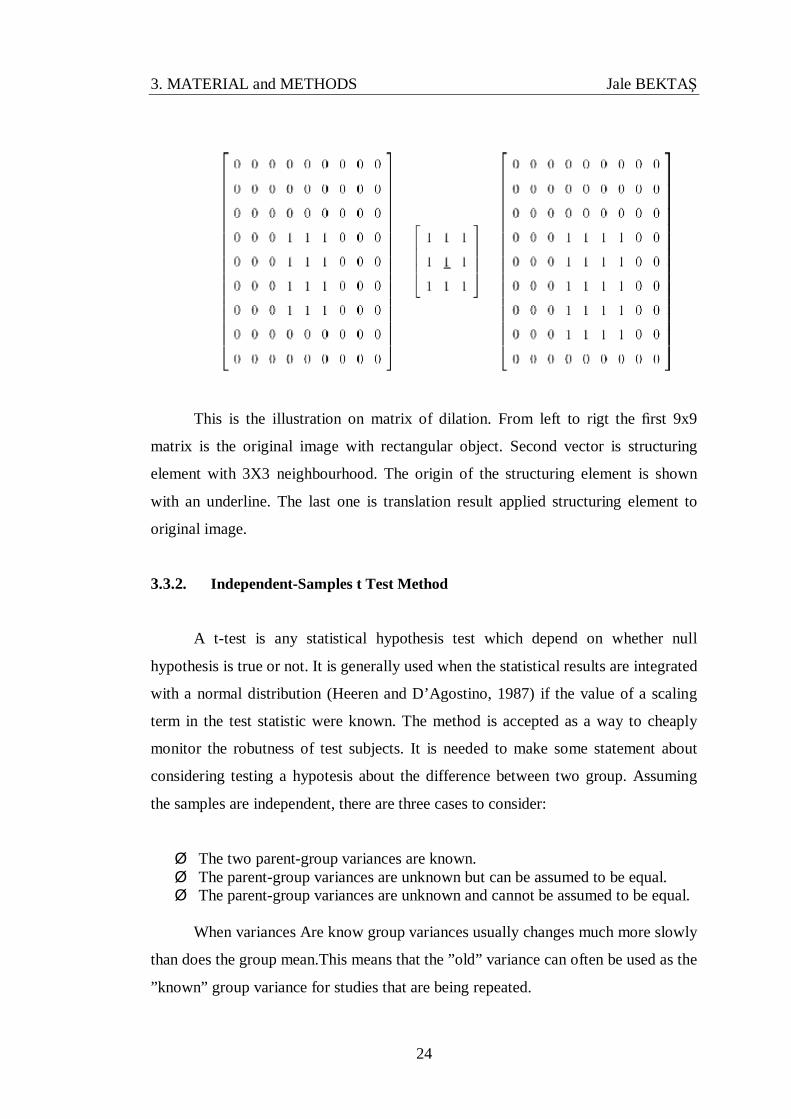
This is the illustration on matrix of erosion. From left to rigt the first 9x9

matrix is the original image with rectangular object. Second vector is structuring

element with 3 neighbors. The origin of the structuring element is shown with an

underline. The last one is translation result applied structuring element to original

image.

Figure 3.4. Erosion example on MRI. From left to rigt the first one is the original image. Second

image is the result after Erosion applied 7x7 neighbourhood

3.3.1.2. Dilation

By this operation, holes in objects are removed and objects consisting of

pixels expand. The rule for dilation is, if any pixel in the input pixels neighbourhood


23

is on, the output pixel is on. Otherwise, the output pixel is off; so dilation, in general,

causes objects in the image to grow in size. Computationally, structuring elements

typically are represented by a matrix of 0s and 1s; sometimes it is conventient to

show only the 1s. In addition, the origin of the structuring element must be clearly

identified.

If set A or B evaluated as an image, A may be considered as the original

image and B may be considered structuring element.

( , ) = ⊕ = ( + )

− = − |

In words, the dilation of A by B is the set consisting of all the structuring

element origin location where the reflected and translated B overlaps at least some

portion of A. Dilation is commutative; that is, ⊕ = ⊕ . If the first operand is

image the second operand must be the structuring element, which usually much

smaller than the image.

Figure 3.5. Dilation example on segmented MRI. From left to rigt the first one is the original

image. Second image is the result after Dilation applied 7x7 neighbourhood


24

This is the illustration on matrix of dilation. From left to rigt the first 9x9

matrix is the original image with rectangular object. Second vector is structuring

element with 3X3 neighbourhood. The origin of the structuring element is shown

with an underline. The last one is translation result applied structuring element to

original image.

3.3.2. Independent-Samples t Test Method

A t-test is any statistical hypothesis test which depend on whether null

hypothesis is true or not. It is generally used when the statistical results are integrated

with a normal distribution (Heeren and D’Agostino, 1987) if the value of a scaling

term in the test statistic were known. The method is accepted as a way to cheaply

monitor the robutness of test subjects. It is needed to make some statement about

considering testing a hypotesis about the difference between two group. Assuming

the samples are independent, there are three cases to consider:

Ø The two parent-group variances are known. Ø The parent-group variances are unknown but can be assumed to be equal. Ø The parent-group variances are unknown and cannot be assumed to be equal.

When variances Are know group variances usually changes much more slowly

than does the group mean.This means that the ”old” variance can often be used as the

”known” group variance for studies that are being repeated.


25

3.3.2.1. Variances Are Unknown

This test is used only when the two population variances are assumed to be

different (the two sample sizes may or may not be equal) and hence must be

estimated separately. The t statistic to test whether the population means are

different can be calculated as follows: = −

When the two parent-group variances are unknown, the standart error of the

test statistic is also unknown, since and are unknown and have to be

estimated. The sample standart deviations are used to estimate the group standart

deviations;

= ∑ ( − ) ( − 1)

the number, n, of participants of each group. This equation is used to estimate σ and = ∑ ( − ) ( − 1)

is used to estimate σ , and the estimates of the standart error of the means become

= √ and = √

If the distibution of the variable in each group can further be assumed to be normal, the appropriate test statistic is

= ( ) − ( )


26

where s is the sample standard deviation of the sample and n is the sample size. The degrees of freedom used in this test is n − 1.

4. WORK STAGES OF STUDY Jale BEKTAŞ

27

4. WORK STAGES OF STUDY

4.1. Feature Selection

The choice of features was selected by observing the images exploring the

dicom header files. In the first stage conditions were placed that autistic and control

subjects had to be at the same sequences and for the homogenity and reliability, 3D

data pixels had to show the same characteristics and shortly these five features were

necessary:

All MRI scans were obtained on a 1.5 T General Electric Signa system(GEs

Signa HDxt 1.5T), using a protocol, includes spoiled gradient recalled echo in steady

state (SPGR).These protocols provide to obtain 3D Fast spin echo (FSE) imaging

sequence sagittal series. Both for images belong to autistic and control subjects have

same sequence and anatomical plane.

1. Same size of rows and columns

All the images have the feature of 256 rows and 256 columns.

2. Slice count in the 3D image matrix

For per 3D image matrix consist of 50 images.

3. Slice thickness information for the images

This feature defines the nominal slice thickness, in mm. Images contain 1.5

mm of slice tickness.

4. Pixel spacing information for the images

This feature defines the physical distance in the image between the center of

each pixel, specified by a numeric pair adjacent row spacing(delimiter),

adjacent column spacing in mm. Images contain [1.015625 1.015625] mm of

pixel spacing values.

5. Voxel Size homogenity for the 3D image matrix

Pixel spacing and slice tickness values form voxel size and these value’s

together homogenity is important to volumetric measurements.

Moreover to be able to success different types of sequences images it must be

achieved to extract features exploring the histograms; so the work focuses in the area


28

of medical image analysis firstly segmentating of these images. Identifying

anatomical structures and labeling interested individuals correctly, segmentation and

matching processes would have been more successful.

The ability to identify anatomical planes is a source of considerable variation

in procedures, because all patient and control subject heads are viewed as

homogeneous. The identification of a set of patient specific landmarks, established a

repeatable 3D coordinate system.

It was written using MATLAB environment that would be able to locate and

label these landmarks working on different sequences MRI head datasets. It would be

more effective using a program which finds the interested regions in 3D data is more

effective than the picking the interested regions on a 2D touch screen representation.

2D rendering of a 3D object has the risk to miss the important portions of soft

tissues. So an automated voxel-based technique would be more effective and

sensitive with the non parametric structure; but considering the difficulites to obtain

standard image intensity information for all image series, a semi automated

technique is preferred.

For the comparisons and detection the following steps are executed image

datasets belong to for all autistic and control groups .

4.2. Descriptions of Program Algorithm Steps

The details of algorithm steps are further given below.

1. Read DICOM Files

This process involves different steps. For dicom loading multiply file selection

is enabled and the program try to produce a whole volume for image analysis.

Investigations is supported in the case of dicom and the header informations in this

structure are the specific pieces of metadata are used (e.g. pixel spacing,flip angle,

the size, number of bytes, class of data, the size of the pixels).

2. Exploring the 3D Data


29

The next step in the algorithm is to explore the 3D data. The purpose of this

step is to consider the images which are relevant to the general interest of the subject.

In this stage 3D histograms are preferred and it was keeped the right to choose to

view an individual slice by entering the slice number. These individual 2D images

can be viewed in grayscale.

3. Segmentation

In this section of the program, the purpose is to segment out the area, or data

of interest.

Ø For the first segmentation step, global and adaptive thresholding techniques

were used depend on the general characteristic of the 3D image data

background.

Ø The next step in the segmentation portion of this program is some manual

thresholding to remove unwanted portions of the image data; low levels like

Cerebral Spinal Fluid.

Ø K-means algorithm was used to segment brain mass to extract other tissues. k

value was 3.

Ø To supply if there are any small wisps of soft tissue in the image, erosion

operation was used with structuring element with 7x7 neighbourhood .

Ø Obtained brain mass is isolated. To grow back the brain mass which was

reduced previously with the erosion, dilation operation was used again with

structuring element with 7x7 neighbourhood .

Ø To catch the connected regions brain region was labelled. This operation also

supplied to control the boundries.

Ø Last segmentation step is choosing significant labeled resulting image slices

from the 3D data set superimposed on original image was evaluated.

4. Volumetric Measurements After Segmentation

Obtained segmented slices are saved. In file saving only the most important

header information is transferred which defines the volume. Segmentation slices

saved as given standart parameters like pixel spacing and slice tickness. These slices


30

combined again to 3D matrix and with k-means 3 portions for WM, GM and

background were found. Parameter for k value was 3.

Density calculations, proportioning volumetric measurements to brain volume,

gray fraction and white fraction were obtained. Information about pixel size and slice

thickness were used during these calculations.

5. Independent Samples t-Test

To measure the reliability, obtained results sent out to Independent Samples t-

Test method and results have been represented .


31

Figure 4.1. Flowchart of Study


32

Figure 4.2. Histogram Distributions of 3D sample images. (a) The histogram of sample image,

belongs to adolescent with autism from Figure 4:5; (b) The histogram of sample

image, belongs to adolescent without autism(Selected from control subject database).

4.3. Visualization Results of Segmentation Application

To obtain segmented volumes, MRI scan data were explored for the properties

of anatomical volumes of 3D renderings. For the segmentation into gray and white

matter regions, intensity based tissue classification of MR images consisted of

histogram thresholding techniques were applied. Semiautomated thresholding

procedure supported with automated global thresholding and manual threshold

values to extract skull, scalp and CSF were used for segmenting brain. To override

for choosing the best threshold values, investigating histogram for each

neuroimaging set, a variety of testing values were used. For a reasonably effective

result thresholding, test values operated for each voxel and a comparison being made

between the obtained resulting image and original image. We are interested in

different regions and consider valley points and compute average value for

background and other parts and explore variations differ from average value. We

used a simply iterative method to not suffer from image noise.


33

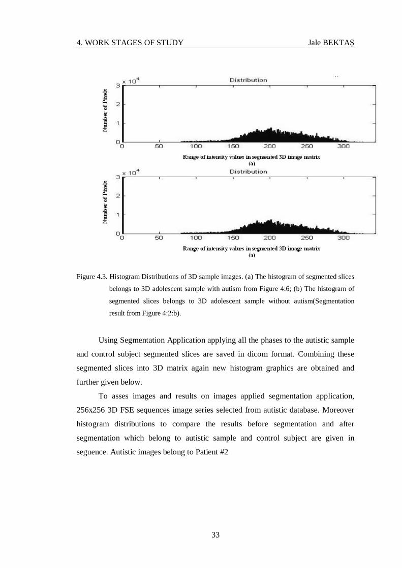
Figure 4.3. Histogram Distributions of 3D sample images. (a) The histogram of segmented slices

belongs to 3D adolescent sample with autism from Figure 4:6; (b) The histogram of

segmented slices belongs to 3D adolescent sample without autism(Segmentation

result from Figure 4:2:b).

Using Segmentation Application applying all the phases to the autistic sample

and control subject segmented slices are saved in dicom format. Combining these

segmented slices into 3D matrix again new histogram graphics are obtained and

further given below.

To asses images and results on images applied segmentation application,

256x256 3D FSE sequences image series selected from autistic database. Moreover

histogram distributions to compare the results before segmentation and after

segmentation which belong to autistic sample and control subject are given in

seguence. Autistic images belong to Patient #2


34

Figure 4.4. Visual comparisons of slices from autistic and control subject database. (a)Control

Subject. (b)Autistic Subject. (c)Segmented image of control subject. (d)Segmented

image of autistic subject

To compare two group selecting two sample image one for autistic group and

the other for control group were demonstrated further. After segmentation process,

results were given under original images.

Comparings were structed on sagittal planed images between autistic and

control subject besides, Coronal T1 Hippoamy images were used to control whether

the autistic subjects measurements calculated correctly. These sequences of images

only belong to


35

Figure 4.5. 256 x 256 3D FSE sequences image series belong to autistic database (Patient #2).


36

Figure 4.6. Segmentation results for per image from Figure 4.5.


37

Figure 4.7. Segmented results from Figure 4.6. superimposedFoingure 4.5. Indicated the

boundaires of segmented regions on the original image


38

autistic database. Control subjects didnt have this type of image datasets. Some

important specifications of images are:

Ø Slice tickness is 0.7

Ø Pixel spacing is [0.937500 0.937500]

Processing the segmentation algorithm for preprocessing step, the background

of 3D fast spin echo images does not have a uniform illumination; so adaptive

thresholding is more successfull to reduce noise. But during the extraction stage of

background of Coronal T1 Hippoamy images, global thresholding process

approximately gets expected results as well as adaptive thresholding. Moreover to

eliminate low positions, observations during exploring histogram get importance.

This parameter must be changed during segmentation. Except this parameter, all

steps for segmentation Coronal T1 Hippoamy images process same as 3D fast spin

echo images.

50 sagittal planed slices selected from autistic database that belong to

Patient#2. Before segmentation in Figure 4.5., after segmentation brain mass in

Figure 4.6. and finally superimposed images which boundries applied on original

images in Figure 4.7. were placed on further pages.

Following these results, 50 Coronal planed slices selected from autistic

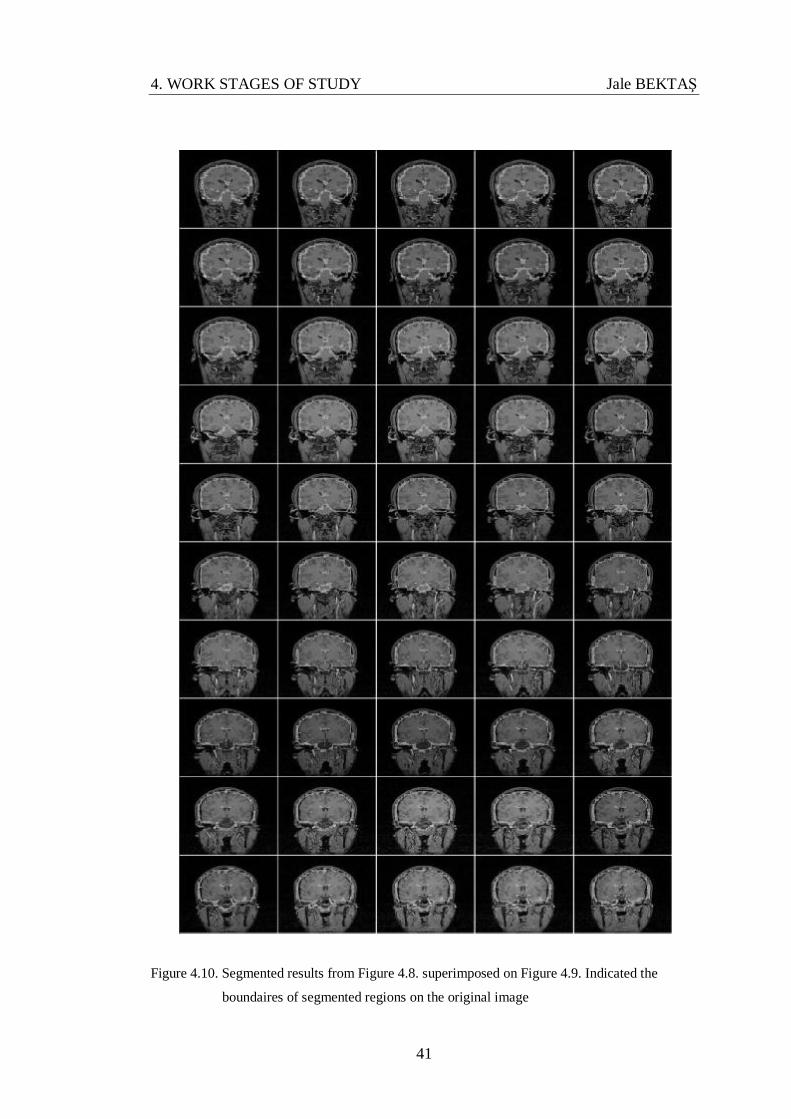
database that belong to Patient #3. Before segmentation in Figure 4.8., after

segmentation brain mass in Figure 4.9. and finally superimposed images which

boundries applied on original images in Figure 4.10. were placed on pages after 3D

FSE images.


39

Figure 4.8. 256x256 Coronal T1 Hippoamy sequences image series belong to autistic database

(Patient #2).


40

Figure 4.9. Segmentation results for per image from Figure 4.8.


41

Figure 4.10. Segmented results from Figure 4.8. superimposed on Figure 4.9. Indicated the

boundaires of segmented regions on the original image

5. EXPERIMENTIAL RESULTS Jale BEKTAŞ

42

5. EXPERIMENTAL RESULTS

5.1. Volumetric Measurements

Control subjects with no history or family history of neurological disorders or

psychiatric illness, consist of 17 years old females and at the same gender disorder

group were placed to participate in the study. Both the control and autistic

participants were female. Control group that is consist of adolescents and young

adults is socioeconomically comparable to based on the family of autistic subjects.

With these clinical criterias neurological history and physical search were the basis

to exclude the autism from other categories of the pervasive developmental disorders

like Asperger syndrome, Childhood disintegrative disorder, Rett syndrome and PDD

not otherwise specified.

In this structural brain imaging study some factors effect the reliability like

less but homogeneous samples, gender, age homogeneity and correspondingly

having Standard genus of accompanying neurological disease (Only autistic

samples). In structural studies when evaluating volume differences, volume increase,

decrease or detection of no significant differences does not provide direct

information related to the functionality of those areas.Together with these parameters

autistic and control groups were compared on WM, GM and total brain volume in

order to test that brain enlargement would continue for adolescents in the age group

of 17 years old. Valley points can be seen according to histogram from Figure 4.2.

There is little jumping area for autistic group and though volume difference is small

it may be reviewed that it is caused from soft tissue largeness.

Volumetric measuments were calculated firstly founding brain voxels and

using voxel size that obtained from dicom files informations brain volume was

extracted and founding gray voxels and using voxel size again that obtained from

dicom files informations gray volume was extracted. Moreover making same

calculations, white volume was obtained. Results for all patients who are diagnosed

with autism and control subjects are given in Table 5.1. and Table 5.2.


43

Table 5.1. Volumetric Measurements of Autistics

Patient Number Total Brain

Volume(liters) GM

Volume(liters) WM

Volume(liters) Patient # 1 1.2881 1.1779 0.1117 Patient # 2 1.2857 1.1183 0.1674 Patient # 3 1.3000 1.1125 0.1881 Patient # 4 1.2941 1.1261 0.1680 Patient # 5 1.2917 1.1521 0.1396

Table 5.2. Volumetric Measurements of Control Subjects

Control Subject

Number Total Brain Vol.(liters)

GM Vol.(liters) WM Vol.(liters)

Control Sub. # 1 1.2624 1.1589 0.1035 Control Sub. # 2 1.2916 1.2439 0.0487 Control Sub. # 3 1.2771 1.1645 0.1126 Control Sub. # 4 1.2689 1.1305 0.1384 Control Sub. # 5 1.2849 1.0956 0.1893 Control Sub. # 6 1.2991 1.1408 0.1583 Control Sub. # 7 1.2256 1.0416 0.1596 Control Sub. # 8 1.3143 1.1710 0.1433 Control Sub. # 9 1.2211 1.0305 0.1906

Control Sub. # 10 1.2719 1.0941 0.1778 Table 5.3. Proportioning Results of Autistics

Patient Number GM/Total Brain

Volume WM/Total Brain

Volume Patient # 1 0.914 0.087 Patient # 2 0.871 0.130 Patient # 3 0.855 0.145 Patient # 4 0.870 0.129 Patient # 5 0.891 0.108


44

Table 5.4. Proportioning Results of Control Subjects

Control Subject Number GM/Total Brain

Volume WM/Total Brain

Volume Control Subject # 1 0.918 0.082 Control Subject # 2 0.963 0.023 Control Subject # 3 0.911 0.088 Control Subject # 4 0.890 0.107 Control Subject # 5 0.853 0.147 Control Subject # 6 0.878 0.122 Control Subject # 7 0.849 0.130 Control Subject # 8 0.890 0.109 Control Subject # 9 0.843 0.156

Control Subject # 10 0.860 0.139

After acquired measuments a simple calculation were made to find gray

fractions and white fractions. For white fraction white volume values are

proportioned to brain volume values. For gray fractions gray volume values are

proportioned to brain volume values. These values are used from Table 5.1. and

Table 5.2.; Table 5.3. results are extracted from Table 5.1.; Table 5.4. results are

extracted from Table 5.2.


45

5.2. T-test Analysis Results

For testing the results, independent sample t-tests analysis were used both

WM, GM and whole brain volume. There are MRI studies which support brain

volume increase in the older year group (Courchesne et al., 2001), (Boddaert et al.,

2009) of autism disorder. For our age group there was no significant difference

(p=0.65) figured for total brain volume between the control group and autism from

Figure 5:1.

For the assessment of WM and GM are ; for the aspect of GM it was fixed that

autistic subjects did not differ from control subjects with an admissible t-test result

(p=0.76) but difference in WM is significance, larger WM volume was determined.

For the comparisons of GM to WM, smaller ratio of white to gray matter was

appeared. These results suggests that this approximation is due to the decrease in

brain volume for the adolescents with autism and increase in brain volume with

control subjects. This approximation may be due to the decrease in brain volume for

the adolescents with autism and increase in brain volume with control subjects. It

may be a mark that the present difference would be closed up with time. Altough a

slight difference was observed through our findings. The results demonstrate that

WM difference underlying this effect.

Table 5.5. Volume comparisons between autistic samples and control group

Values of volume,mL BRAIN REGION Mean ± SD p value for t-test

WM 0.18 Autism 154,9.0 ± 39.2 Control 144,1.0 ± 31.1 GM 0.76 Autism 1,137.0 35.6 Control 1,120.9 110.5 Total brain 0.65 Autism 1,291.9 ± 78.00 Control 1,265.0 ± 89.20

±±


46

Moreover comparings were structed on sagittal planed images between

autistic and control subject besides, Coronal T1 Hippoamy images were used to

control whether the autistic subjects measurements calculated correctly. For same

databases there were no significant differences between volumetric results that

acquired from Coronal T1 Hippoamy images and Sagittal 3D FSE images. This

observations advanced the reliability of segmentation application.

6. CONCLUSION Jale BEKTAŞ

47

6. CONCLUSION

This study was based on to develop a method which detects autism with an

effective and very simple way. To carry this theory of this study to the real life, we

processed MRI images automatically and got expected results. The study prevents

vasting time to explore data manually, works rather fast, provides very significant

savings in material andthe most important thing is that it is structured to determine

disease in every terms. At theend of this thesis, prepared study must be assessed in

two stages.

For the first stage, k-means algorithm was programmed to use processed 3-D

MR image slices as input signals. The use of k-means with partial image processing

techniques allowed segmenting brain shape of a human consisted of a set of magnetic

resonance images. Finally a segmentation algorithm has been revealed. Through this

process, certain structures of the image like the holes in the brain mask and non-brain

objects that form a round shape constitution around the brain mask are discarded.

These steps pay attention to the boundary of the brain so that it could not be

interrupted and continuously fills all the holes that lie within the boundary of the

main brain.

For the second stage, the study was reviewed for the effects of 17 years old

adolescents and approximation of brain volume in the autism group to control

subjects was determined. The output has been determined as comparison results

between the adolescents who have typical development and have autism diagnostic.

According to the comparison results, there was no significant difference figured for

total brain volume between the control group and autism and also GM to WM,

smaller ratio of white to gray matter was appeared. For the assessment of WM and

GM are; for the aspect of GM, it was fixed that autistic subjects did not differ from

control subjects but difference in WM is significance, larger WM volume was

determined.

The study suggests that this approximation is due to the decrease in brain

volume for the adolescents with autism and increase in brain volume with control

subjects. It may be a mark that the present difference would be closed up with time.

6. CONCLUSION Jale BEKTAŞ

48

However medical investigations shows that the volume difference disappers in adult

term in life. Altough a slight difference was observed through our findings. The

results which acquired from this application demonstrate that WM difference is the

reason underlying this effect. So we can say that this study is a sample to detect brain

measurement comparisons between different groups using MRI.

49

REFERENCES

ABELL, F., KRAMS, M., ASHBURNER, J., PASSINGHAM, R., FRISTON, K.,

FRACKOWIAK, R., HAPP´E, F., FRITH, C.,, and FRITH, U., 1999. The

neuroanatomy of autism: a voxel-based whole brain analysis of structural

scans. Neuroreport, 10(8):1647.

AYLWARD, E., MINSHEW, N., FIELD, K., SPARKS, B.,, and SINGH, N., 2002.

Effects of age on brain volume and head circumference in autism. Neurology,

59(2):175.

BEKTAS, J., and IBRIKCI, T., 2009. Using Threshold Techniques with K-Means

Approach for MRI Segmentation. In The 2009 International Conference on

Image Processing, Computer Vision, and Pattern Recognition. Worldcomp.

BODDAERT, N., ZILBOVICIUS, M., PHILIPE, A., ROBEL, L., BOURGEOIS,

M., BARTHELEMY, C., SEIDENWURM, D., MERESSE, I., LAURIER, L.,

DESGUERRE, I.,, et al., 2009. MRI findings in 77 children with non-

syndromic autistic disorder. PLoS ONE, 4(2).

BROWN, M., and SEMELKA, R., 1999. MR Imaging Abbreviations, Definitions,

and Descriptions: A Review1. Radiology, 213(3):647.

CARPER, R., MOSES, P., TIGUE, Z.,, and COURCHESNE, E., 2002. Cerebral

lobes in autism: early hyperplasia and abnormal age effects. Neuroimage,

16(4):1038–1051.

CHEUNG, Y., 2003. k-means: a new generalized k-means clustering algorithm

Pattern Recognition Letters, 24(15):2883–2893.

COURCHESNE, E., 2004. Brain development in autism: early overgrowth followed

by premature arrest of growth. Mental Retardation and Developmental

Disabilities Research Reviews, 10(2):106–111.

COURCHESNE, E., KARNS, C., DAVIS, H., ZICCARDI, R., CARPER, R.,

TIGUE, Z., CHISUM, H., MOSES, P., PIERCE, K., LORD, C.,, et al., 2001.

Unusual 42 brain growth patterns in early life in patients with autistic

disorder: an MRI study. Neurology, 57(2):245.

50

COURCHESNE, E., REDCAY, E.,, and KENNEDY, D., 2004. The autistic brain:

birth through adulthood. Current Opinion in Neurology, 17(4):489.

EIGSTI, I., and SHAPIRO, T., 2003. A systems neuroscience approach to autism:

biological, cognitive, and clinical perspectives. Mental retardation and

developmental disabilities research reviews, 9(3):206–216.

GONZALEZ, R., C., and WOODS, R., E., 2002. Digital image processing, 2. Ed.

Prentice-Hall Inc., New Jersey.

GRAHAM, R., PERRISS, R.,, and SCARSBROOK, A., 2005. DICOM demystified:

a review of digital file formats and their use in radiological practice. Clinical

Radiology, 60(11):1133–1140.

HAZLETT, H., POE, M., GERIG, G., SMITH, R.,, and PIVEN, J., 2006. Cortical

gray and white brain tissue volume in adolescents and adults with autism.

Biological Psychiatry, 59(1):1–6.

HEEREN, T., and D’AGOSTINO, R., 1987. Robustness of the two independent

samples t-test when applied to ordinal scaled data. Statistics in medicine,

6(1):79–90.

HORNAK, J., 2010. The basics of MRI. Disponvel em¡ http://www. cis. rit.

edu/htbooks/mri. Acesso em, 8.

KANNER, L., et al., 1943. Autistic disturbances of affective contact. Nervous child,

2(217.250).

KHALIGHI, M., SOLTANIAN-ZADEH, H.,, and LUCAS, C., 2002. Unsupervised

MRI segmentation with spatial connectivity. In Proceedings of the SPIE

International Symposium on Medical Imaging. Citeseer.

LAINHART, J., 2006. Advances in autism neuroimaging research for the clinician

and geneticist. month, 1:2.

LAINHART, J., PIVEN, J., WZOREK, M., LANDA, R., SANTANGELO, S.,

COON, H.,, and FOLSTEIN, S., 1997. Macrocephaly in children and adults

with autism. Journal of Amer Academy of Child & Adolescent Psychiatry,

36(2):282.

51

LAKARE, S., and KAUFMAN, A., 2000. 3D segmentation techniques for medical

volumes. Center for Visual Computing, Department of Computer Science,

State University of New York.

LI, X., TSO, S., GUAN, X.,, and HUANG, Q., 2006. Improving automatic detection

of defects in castings by applying wavelet technique. IEEE Transactions on

Industrial Electronics, 53(6):1927.

LINGURARU, M., VERCAUTEREN, T., REYES-AGUIRRE, M., BALLESTER,

M.,, and AYACHE, N., 2007. SEGMENTATION PROPAGATION FROM

DEFORMABLE ATLASES FOR BRAIN MAPPING AND ANALYSIS.

LORD, C., RUTTER, M.,, and COUTEUR, A., 1994. Autism Diagnostic Interview-

Revised: a revised version of a diagnostic interview for caregivers of

individuals with possible pervasive developmental disorders. Journal of

Autism and Developmental Disorders, 24(5):659–685.

MCALONAN, G., DALY, E., KUMARI, V., CRITCHLEY, H., AMELSVOORT,

T., SUCKLING, J., SIMMONS, A., SIGMUNDSSON, T., GREENWOOD,

K., RUSSELL, A.,, et al., 2002. Brain anatomy and sensorimotor gating in

Asperger’s syndrome. Brain, 125(7):1594.

MINGOTI, S., and LIMA, J., 2006. Comparing SOM neural network with Fuzzy c-

means, K-means and traditional hierarchical clustering algorithms. European

Journal of Operational Research, 174(3):1742–1759.

PAL, N., and PAL, S., 1993. A review on image segmentation techniques. Pattern

recognition, 26(9):1277–1294.

PHAM, D., XU, C.,, and PRINCE, J., 2000. C URRENT M ETHODS IN M

EDICAL I MAGE S EGMENTATION 1. Annual Review of Biomedical

Engineering, 2(1):315–337.

ROBINS, D., FEIN, D., BARTON, M.,, and GREEN, J., 2001. The Modified

Checklist for Autism in Toddlers: An initial study investigating the early

detection of autism and pervasive developmental disorders. Journal of Autism

and Developmental Disorders, 31(2):131–144.

52

SCHUMANN, C., HAMSTRA, J., GOODLIN-JONES, B., LOTSPEICH, L.,

KWON, H., BUONOCORE, M., LAMMERS, C., REISS, A.,, and

AMARAL, D., 2004. The amygdala is enlarged in children but not

adolescents with autism; the hippocampus is enlarged at all ages. Journal of

Neuroscience, 24(28):6392.

SPARKS, B., FRIEDMAN, S., SHAW, D., AYLWARD, E., ECHELARD, D.,

ARTRU, A., MARAVILLA, K., GIEDD, J., MUNSON, J., DAWSON, G.,,

et al., 2002. Brain structural abnormalities in young children with autism

spectrum disorder. Neurology, 59(2):184.

ULAY, H., and ERTUGRUL, A., 2009. Otizmde Beyin Goruntuleme Bulgular: Bir

Gozden Gecirme. Journal, Turkish Psychiatry.

UNIVERISTY, T., 2001. A statistical 3-D segmentation algorithm for classifying

brain tissues in multiple sclerosis. In Proceedings, 14th IEEE Symposium on

Computer-Based Medical Systems: CBMS 2001: 26-27 July 2001, Bethesda,

Maryland, page 455. IEEE.

WANG, Y., ADALI, T., KUNG, S.,, and SZABO, Z., 1998. Quantification and

segmentation of brain tissues from MR images: A probabilistic neural

network approach. IEEE transactions on image processing: a publication of

the IEEE Signal Processing Society, 7(8):1165.

WIDIGER, T., and SAMUEL, D., 2005. Diagnostic Categories or Dimensions? A

Question for the Diagnostic and Statistical Manual of Mental DisordersFifth

Edition. Journal of Abnormal Psychology, 114(4):494–504.

53

CURRICULUM VITAE

I was born in Adana, Turkey in 1979. I graduated from Mersin Universty, Department of Computer Engineering in 2002 and I have been working as lecturer in Erdemli School of Applied Technology and Business since December 2005.

institute of natural and applied ... - library.cu.edu.tr · since its recognition by leo kanner in...

Documents