IMES DISCUSSION PAPER SERIES

INSTITUTE FOR MONETARY AND ECONOMIC STUDIES

BANK OF JAPAN

2-1-1 NIHONBASHI-HONGOKUCHO CHUO-KU, TOKYO 103-8660

JAPAN

You can download this and other papers at the IMES Web site:

https://www.imes.boj.or.jp

Do not reprint or reproduce without permission.

The Implied Bail-in Probability in

the Contingent Convertible Securities Market

Masayuki Kazato and Tetsuya Yamada

Discussion Paper No. 2018-E-3

NOTE: IMES Discussion Paper Series is circulated in order to stimulate discussion and comments. Views expressed in Discussion Paper Series are those of authors and do not necessarily reflect those of the Bank of Japan or the Institute for Monetary and Economic Studies.

IMES Discussion Paper Series 2018-E-3 May 2018

The Implied Bail-in Probability in

the Contingent Convertible Securities Market

Masayuki Kazato* and Tetsuya Yamada**

Abstract

The issuance of contingent convertible securities (CoCos) has increased not only in Europe but also in Asia and other areas over the past several years. In this paper, we extend the existing model used to price CoCos to estimate the implied bail-in probability for a variety of CoCos by modifying loss rates for investors due to bail-ins of CoCos. Using our model for empirical analyses, we find that when the credit events occur, the bail-in probability of a CoCo increases by more than the default probability implied by credit default swaps (CDS). The result suggests that the bail-in probability can be used as an early warning indicator of financial crises. We also find that the conditional default probability after bail-in tends to be lower the more CoCos a bank has issued. This finding indicates that investors believe financial institutions become less likely to default as issuing more CoCos strengthens their loss absorption capacity. Overall, our analysis suggests that the market prices of CoCos contain useful information on financial stability. Keywords: Market-implied bail-in probability; Contingent convertible securities;

Basel III; Financial stability JEL classification: G12, G15, G21, G28, G32, G33

* Deputy Director, Institute for Monetary and Economic Studies, Bank of Japan (E-mail: masayuki.kazato@boj.or.jp)

** Director, Institute for Monetary and Economic Studies (currently Financial System and Bank Examination Department), Bank of Japan (E-mail: tetsuya.yamada@boj.or.jp)

The authors would like to thank Tjeerd M. Boonman (Banco de México), Hidetoshi Nakagawa (Hitotsubashi University), Mana Nakazora (BNP Paribas Securities (Japan) Limited), Kenji Ogawa (Bloomberg L.P.), Sriram Rajan (Office of Financial Research), Hajime Suwa (Mitsubishi UFJ Morgan Stanley Securities Co., Ltd.) and his staff, Edward Tan (Hong Kong Monetary Authority), participants of the 10th Annual Workshop of the Asian Research Network and the Second Conference on Network Models and Stress Testing for Financial Stability, and the staff of the Institute for Monetary and Economic Studies, Bank of Japan, for useful comments. All remaining errors are our own. The views expressed in this paper are those of the authors and do not necessarily reflect the official views of the Bank of Japan.

1. Introduction

Since 2009, large financial institutions have dramatically increased their issuance of contingent convertible securities (CoCos)—securities that are convertible into equity or whose principal is reduced when the issuer’s capital ratio falls below a certain level. While CoCos were initially issued by European banks alone, they are now issued by financial institutions in various parts of the world, including South America and Asia/Oceania (Figure 1, 2, Table 1). Today, almost all the global systemically important banks (G-SIBs) except those in the U.S. issue these new hybrid securities (Table 2).

There are two main reasons for the increasing popularity of CoCos among G-SIBs. First, global banks face the need to strengthen their capital to meet the requirements of Basel III. CoCos are a form of bail-in debt that mean that bank losses are absorbed by CoCo holders and thus helps to ensure that banks have ample capital available when they face financial stress. During the recent global financial crisis, the burden imposed on tax payers as a result of the bail-out of, and injection of public funds into, financial institutions led to massive criticism. CoCos were designed to prevent such bail-outs in the future. Second, CoCos offer relatively high yields to compensate for possible bail-in in the future. Under the current environment of low interest rates in many advanced economies, the relatively high yields provided by CoCos are attractive to a wide range of investors.

In February 2016, the spreads between CoCos and government bonds jumped due to concern over the soundness of a European financial institution (the so-called Deutsche Bank shock). The jump in spreads reflected investors’ perception that bail-ins were more likely to occur. This episode has led market participants and financial regulators to pay closer attention to the dynamics of CoCo spreads.

In addition to the risk of the issuer’s default, CoCo spreads reflect the risk of bail-in and the fact that a bail-in will be triggered before a default. As a result, such spreads are likely to respond more to the issuer’s capital soundness than to credit spreads. If that is the case, CoCo spreads could be utilized as an early warning indicator for individual financial institutions as well as the financial system overall.

In this paper, we modify an existing model used to price CoCos to estimate the implied bail-in probability from the price of CoCos. We then apply these probabilities for various analyses related to financial stability.

Previous studies proposed several methods of pricing CoCos. Wilkens and Bethke

1

(2014) classify such pricing methods into two groups: structural methods and derivatives methods.1,2 The first method incorporates the dynamics of the value of assets held by a financial institution and assesses the value of a CoCo by examining whether the assets and liabilities on the issuing institution’s simplified balance sheet are consistent with each other. This approach is adopted in studies analyzing the incentive structure of bank shareholders and creditors as well as the theoretical effects of the issuance of CoCos for the financial system. The second method puts more emphasis on the assessment of the put option characteristics of CoCos. This is the approach adopted in most empirical studies on CoCos, since it incorporates parameters that are available in financial markets and makes estimation relatively simple. In this paper, we follow the derivatives method to evaluate the value of CoCos and to estimate the bail-in probability of CoCos, that is, the probability that a bail-in event occurs over a certain period of time in the future.

There are relatively few studies on the issue of bail-in probabilities, which reflect investors’ belief about the likelihood that a bail-in even occurs in the future, estimated from the price of a CoCo. A notable exception is the study by De Spiegeleer, Dhaene, and Schoutens (2013), who examine the bail-in probability based on the initial issue price of a CoCo issued by a Swiss financial institution. They conclude that the bail-in probably was much higher than investors seem to be believed. However, they do not show their methodology in detail and only present a one-shot result in their short report.3 Another exception is the study by Neuberg et al. (2016), who estimate from credit default swap (CDS) spreads the implied probability of government intervention, which is related to, but different from, our bail-in probability. They use the fact that government intervention was added to CDS credit events since the introduction of the International Swaps and Derivatives Association’s “Credit Derivatives Definitions Protocol” in 2014. Meanwhile, Brigo, Garcia, and Pede (2013) estimated the term structure of the bail-in probability for a particular financial institution at a particular

1 Studies employing the structural approach include Kamada (2010), Pennacchi (2010), Madan and Schoutens (2011), Albul, Jaffee, and Tchistyi (2010), Glasserman and Nouri (2012), Cheridito and Xu (2014), Erismann (2015), Pennacchi and Tchistyiz (2015), Sundaresan and Wang (2015), Vullings (2015), and Song and Yang (2016). 2 Studies employing the derivatives approach include Serjantov (2011), De Spiegeleer and Schoutens (2012, 2014), De Spiegeleer et al. (2017), Corcuera et al. (2013), Teneberg (2012), Chung and Kwok (2016), Erismann (2015), Ritzema (2015), Partanen (2016), Persio, Bonollo, and Prezioso (2016), and Stamicar (2016). 3 Similarly, J.P. Morgan (2014) provides a snapshot result of the bail-in probability for a specific G-SIB.

2

point in time.

The contribution of our study to the literature is threefold. First, we extend an existing pricing model to estimate bail-in probabilities by controlling the diverse characteristics of CoCos. Second, we conduct a comprehensive analysis of the bail-in probability for several banks in various countries using time-series data. Finally, we show that bail-in probabilities could be an early warning indicator of financial crises and that the market prices of CoCos contain useful information on the stability of the financial system.

The rest of the paper is organized as follows. Section 2 presents a standard model used for estimating the implied bail-in probability of CoCos. We extend the model to represent a more realistic setting. Section 3 shows the empirical results for the implied bail-in probabilities and their implications for macro-prudential policy. Section 4 concludes.

2. Method

In this section, we present a standard model for estimating the implied bail-in probability of a CoCo using market data. As mentioned in the introduction, we follow the derivatives method. Specifically, we employ a model based on the credit derivatives approach. In addition, we extend the credit derivatives approach to evaluate bail-in probabilities for CoCos whose principal is reduced to absorb losses incurred by the issuer.

2.1 Estimating the bail-in probability of CoCos with the credit derivatives model

The credit derivatives approach was introduced by De Spiegeleer and Schoutens (2012). The basic idea underlying their model is to calculate, similar to the case of a barrier option, the extra yield required by investors to compensate for the risk of any possible losses. They assume that the CoCo trigger event, which often is set to a fall in the issuer’s Common Equity Tier 1 (CET1) ratio below a certain level, corresponds to a drop in the issuer’s share price below a certain threshold. The threshold is called the trigger share price. Based on this assumption, the model then translates the CoCo’s accounting trigger, which is difficult to measure more frequently than once a quarter, into the market trigger, which can be observed at a higher frequency. The assumption therefore makes it possible to estimate the bail-in probability as the probability of hitting the trigger share price of a knock-in option.

3

To obtain the bail-in probability of CoCos in practice, we need to relate CoCo spreads to bail-in probabilities and to formulate these probabilities based on a standard pricing approach to barrier options. First, we discuss the relationship between CoCo spreads and bail-in probabilities in the credit derivatives approach. The spread, 𝐶𝐶𝑆𝑆𝐶𝐶𝐶𝐶𝐶𝐶𝐶𝐶, is decomposed into a loss rate, 𝐿𝐿𝐿𝐿𝐿𝐿𝐿𝐿𝐶𝐶𝐶𝐶𝐶𝐶𝐶𝐶, and a hazard rate, 𝜆𝜆𝑇𝑇𝑇𝑇𝑇𝑇𝑇𝑇𝑇𝑇𝑇𝑇𝑇𝑇:

𝐶𝐶𝑆𝑆𝐶𝐶𝐶𝐶𝐶𝐶𝐶𝐶 = 𝐿𝐿𝐿𝐿𝐿𝐿𝐿𝐿𝐶𝐶𝐶𝐶𝐶𝐶𝐶𝐶 × 𝜆𝜆𝑇𝑇𝑇𝑇𝑇𝑇𝑇𝑇𝑇𝑇𝑇𝑇𝑇𝑇. (1)

By combining the trigger share price, H, which is the market value of the share at the time of bail-in, and the conversion share price, Cp, which is the face value of the share the CoCo investors acquire, the loss rate is expressed as:4

𝐿𝐿𝐿𝐿𝐿𝐿𝐿𝐿𝐶𝐶𝐶𝐶𝐶𝐶𝐶𝐶 =

𝐶𝐶𝑃𝑃 − 𝐻𝐻𝐶𝐶𝑃𝑃

= 1 −𝐻𝐻𝐶𝐶𝑃𝑃

. (2)

On the other hand, the hazard rate shows the bail-in probability over a short period. When the hazard rate is constant over time, the cumulative bail-in probability for the coming T years, PH, is given by:5,6

𝑃𝑃𝐻𝐻 = 1 − 𝑒𝑒−𝜆𝜆𝑇𝑇𝑇𝑇𝑇𝑇𝑇𝑇𝑇𝑇𝑇𝑇𝑇𝑇𝑇𝑇 ⇔ 𝜆𝜆𝑇𝑇𝑇𝑇𝑇𝑇𝑇𝑇𝑇𝑇𝑇𝑇𝑇𝑇 = −

ln(1 − 𝑃𝑃𝐻𝐻)𝑇𝑇

. (3)

Note that in this paper we will refer to the cumulative bail-in probability as the bail-in probability.

Second, we assume CoCos are regarded as a knock-in option with the barrier at H. The bail-in probability PH is then equal to the probability of hitting the trigger share price H of the knock-in option, as argued by Su and Rieger (2009) :7

4 The trigger share price is unobservable; it is difficult to determine whether the estimated value is appropriate due to the scarcity of bail-in events so far. 5 It could be argued that the hazard rate changes dynamically and the assumption of a constant hazard rate is not appropriate. We deal with this issue to some extent by evaluating the term structure of bail-in probabilities in Section 3.

6 The actual loss rate will depend on when investors sell the stocks obtained through the CoCo conversion, so that realized loss rates may differ across CoCo investors. However, the trigger share price implied by market data can be thought of as including all possible investor loss rates. 7 The probability of hitting the trigger share price of the knock-in option is similar to the probability of hitting a firm’s value going into default introduced by Black and Cox (1976).

4

𝑃𝑃𝐻𝐻 = 𝑁𝑁 �

ln(𝐻𝐻/𝑆𝑆) − 𝜇𝜇𝑇𝑇𝜎𝜎√𝑇𝑇

� + �𝐻𝐻𝑆𝑆�2𝜇𝜇/𝜎𝜎2

𝑁𝑁 �ln(𝐻𝐻/𝑆𝑆) + 𝜇𝜇𝑇𝑇

𝜎𝜎√𝑇𝑇�, (4)

where 𝑆𝑆 is the issuer’s stock price, 𝜎𝜎 is the volatility of the stock price, 𝜇𝜇 is equal to 𝑟𝑟 − 𝜎𝜎2 2⁄ , where 𝑟𝑟 is the risk-free rate, and 𝑁𝑁[∙] is the normal cumulative distribution function.

One sensible estimate of 𝜎𝜎 is the historical volatility of the stock price. However, since 𝜎𝜎 would be higher than usual when a bail-in event occurs, the historical volatility likely underestimates the volatility relevant for quantifying the bail-in probability. Therefore, a better estimate of 𝜎𝜎 is the implied volatility by option with a deep-out-of-the-money strike, whose strike is very far away from at-the-money strike. However, such deep out of the money options are generally not traded in the market (i.e., their liquidity is so thin as to be non-existent). We therefore follow Henriques and Doctor (2011) and use the implied volatility from CDS spreads as our estimate of 𝜎𝜎. As discussed in Appendix 1, Henriques and Doctor (2011) assume that a default occurs when the stock price falls to 5% of the current stock price, which corresponds to a deep-out-of-the-money strike price.

Other than H, all variables to calculate 𝑃𝑃𝐻𝐻 can be observed in the market: S and r are observable, while 𝜎𝜎 can be estimated as described in the previous paragraph. By calibrating equations (3) and (4) using market data, we obtain H and the implied bail-in probability PH at maturity T. 8 This method can be applied to estimate bail-in probabilities for total loss-absorbing capacity (TLAC) bonds.9

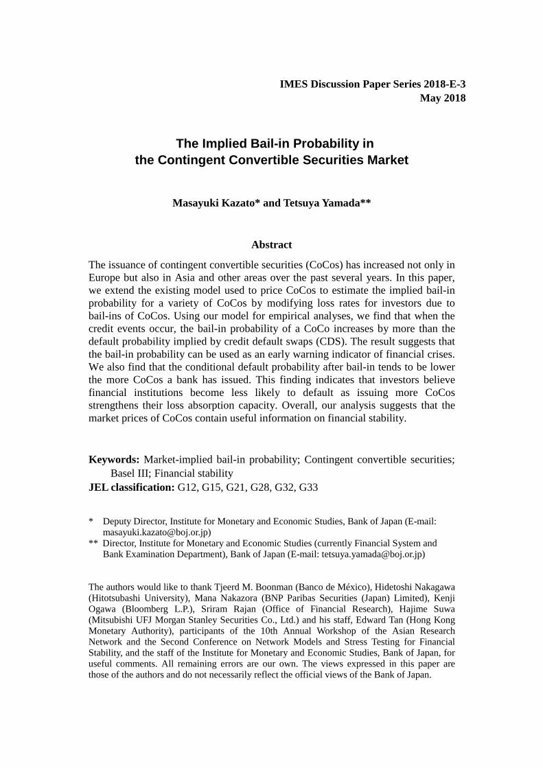
The relationships between PH and its main parameters are shown in Figure 3 to gain an intuitive grasp of the dynamics of PH. For simplicity, we show the result for CoCos with a permanent write-down (LossCoCo=1, as explained in the following subsection). The figure indicates that the implied bail-in probability PH is higher the lower the stock price, the higher the trigger stock price, the higher the stock volatility, and the longer the time to maturity. As Figure 3(d) shows, we calculate the theoretical bail-in probability as a function of T. For our analysis, we set the term to five years. By fixing the term at five years, we can easily compare the bail-in probability with other CoCos issued by

8 Following market practice, we set the parameter T to time-to-maturity or time to the CoCo’s first call. 9 We are unable to perform empirical studies of the bail-in probability for TLAC bonds due to the limited availability of data for such bonds.

5

other banks and also with the default probability implied by five-year CDS spreads.10

Figure 4 shows an example of the estimated bail-in probability of a CoCo with equity conversion issued by a European bank. The solid and dashed lines depict the bail-in probability and the CoCo spread, respectively. The bail-in probability and the CoCo spread often move together. However, they do not always comove, as can be seen in the final three months shown in Figure 4. Specifically, during this period, the bail-in probability increased while the spread did not change. In the period, stock prices in Europe recovered after the Brexit referendum in June 2016. In the meantime, the European Banking Authority published its stress test results for European banks at the end of July 2016, which made investors concerned about financial institutions’ core capital. As a result, the CoCo spread did not fall, while the stock price rose. Hence, the estimated bail-in probability increased, while the spread did not change.

2.2 Extension of the credit derivatives model

In subsection 2.1, we examined the spreads of CoCos that convert into equity at a fixed conversion price. As shown in Figure 5, there are a variety of CoCos in the market. They can be broadly classified into equity conversion and write-down (principal reduction) CoCos. Equity conversion CoCos can be further subdivided into those with a fixed conversion price and those without a fixed conversion price. In Appendix 2, we deal with the equity conversion mechanism without a fixed conversion price, although the model is not used for the empirical analysis in this paper. Write-down CoCos can be further classified into permanent write-down and temporary write-down ones. In the following subsections, we extend the pricing model for equity-conversion CoCos developed in the previous subsection to estimate the bail-in probability for CoCos with permanent write-down and temporary write-down.

2.2.1 Bail-in probability for permanent write-down CoCos

If a CoCo absorbs its issuer’s losses by means of permanent write-down, its principal becomes zero with no possibility to write the principal up again. In this case, the recovery rate equals zero (the loss rate equals one) by definition and the model can be

10 Note that the fixed-term bail-in probabilities for CoCos issued by the same institution with different maturities may differ due to differences in hazard rates across CoCos. In addition, our model assumes that stock prices follow a continuous diffusion process without a sudden change in price. This means that the bail-in probability estimate for a CoCo with a short time to maturity will be extremely small, as shown in Figure 3(d), and maybe be underestimated. Therefore, we use data for CoCos with close to five years to maturity for our analysis below.

6

easily modified by changing the loss rate to one in equation (2), i.e., 𝐿𝐿𝐿𝐿𝐿𝐿𝐿𝐿𝐶𝐶𝐶𝐶𝐶𝐶𝐶𝐶1 = 1. Then, using equation (3), we can write equation (1) as:

𝐶𝐶𝑆𝑆𝐶𝐶𝐶𝐶𝐶𝐶𝐶𝐶1 (𝐻𝐻) ≡ −

ln[1 − 𝑃𝑃(𝐻𝐻)]𝑇𝑇

, (5)

where 𝑃𝑃(𝐻𝐻) is defined as in equation (4).

2.2.2 Bail-in probability for temporary write-down CoCos

A CoCo’s principal can be written up after a write-down when the CoCo is of the temporary write-down type. Coupon payments will be suspended during the period of the write-down. Moreover, the amount of the coupon may be lower after the write-up. To build a model for CoCos with a temporary write-down, it is necessary to deal with the duration of the write-down in the future and also the coupon amount after the write-up. Here, we assume that the coupon payments are zero after the write-up of a CoCo’s principal. This assumption simplifies the issue that the values of the different types of CoCos depend on whether their principals will be fully written down or fully written up at maturity. In the model, we need to take into account whether the share price at maturity will be higher than the trigger share price or not. Thus, the loss rate in equation (2) becomes one and the bail-in probability is equal to the first term of equation (4). As a result, the CoCo spread is equal to the hazard rate when the stock price at maturity is lower than the trigger share price, i.e.:

𝐶𝐶𝑆𝑆𝐶𝐶𝐶𝐶𝐶𝐶𝐶𝐶0 (𝐻𝐻) ≡ −

ln�1 − 𝑃𝑃0(𝐻𝐻)�𝑇𝑇

,

𝑃𝑃0(𝐻𝐻) = 𝑁𝑁 �ln(𝐻𝐻/𝑆𝑆) − 𝜇𝜇𝑇𝑇

𝜎𝜎√𝑇𝑇�.

(6)

On the one hand, it is possible that our simplification leads us to overestimate the value of the CoCo, because we also assume a full recovery of the principal when a write-up occurs, which is the most desirable situation for investors.11 On the other hand, our assumption of no possibility of a write-up for permanent write-down CoCos discussed in the previous subsection represents the worst-case scenario for investors. Therefore, based on our assumptions, the spread for temporary write-down CoCos lies between the spread in equation (5) and the spread in equation (6), i.e.:

11 If we take coupon payments after the write-up into account, we may underestimate the CoCo values and consequently overestimate the bail-in probabilities. However, if the present value of coupons is smaller than the principal repayment of the CoCo, the effect is likely to be limited.

7

𝐶𝐶𝑆𝑆𝐶𝐶𝐶𝐶𝐶𝐶𝐶𝐶0 (𝐻𝐻) ≤ 𝐶𝐶𝑆𝑆𝐶𝐶𝐶𝐶𝐶𝐶𝐶𝐶(𝐻𝐻) ≤ 𝐶𝐶𝑆𝑆𝐶𝐶𝐶𝐶𝐶𝐶𝐶𝐶1 (𝐻𝐻). (7)

Let 𝐻𝐻0 and 𝐻𝐻1 be the trigger share prices obtained by applying equations (5) and (6) for the observed CoCo spread. From equation (7), the relationship among 𝐻𝐻0, 𝐻𝐻1, and the trigger share price H for CoCos with temporary write-down can be expressed as follows:

𝐻𝐻1 ≤ 𝐻𝐻 ≤ 𝐻𝐻0, (8)

This means that we can obtain the bail-in probabilities for CoCos with temporary write-down as a band by substituting those trigger share prices into equation (4):

𝑃𝑃(𝐻𝐻1) ≤ 𝑃𝑃(𝐻𝐻) ≤ 𝑃𝑃(𝐻𝐻0). (9)

In Appendix 3, we also consider an extension of the model assuming that the write-up ratio depends on the relative share price at maturity vis-à-vis the trigger share price.

3. Results and discussion

In this section, we present empirical analyses of the implied bail-in probabilities of CoCos in the market based on our model. Specifically, we first show that the change in bail-in probabilities is larger than that in default probabilities implied by the market CDS spread when investors become worried about the soundness of banks. We then estimate the conditional probabilities of default when the bail-in trigger has already been pulled. These conditional probabilities indicate investors’ assessment of the CoCos’ loss absorption buffer. We also present further analyses such as principal component analysis by region and the term structure of bail-in probabilities.

3.1 The bail-in probability as an early warning indicator of financial crises

We start by comparing the bail-in probabilities implied by CoCos with the default probabilities implied by CDSs. This comparison helps us to confirm one of our hypotheses, namely, that CoCo bail-in probabilities react more strongly than CDS default probabilities to events that may lead to a deterioration in the soundness of banks.

Figure 6 shows the results for selected G-SIBs in Europe. The solid lines and bands depict the bail-in probabilities, and the dashed lines are the default probabilities. We find large differences in the reaction of the two probabilities to certain events highlighted by the circles, namely the stress test carried out by the European Central

8

Bank (ECB) in October 2014 and as well as mounting concern over the soundness of Deutsche Bank in February 2016. 12 , 13 , 14 This suggests that the implied bail-in probability could serve as an early warning indicator of financial crises.15 On the other hand, almost no difference in the response of CoCo bail-in probabilities and CDS default probabilities to the Brexit referendum in June 2016 can be observed. A possible reason is that any risk posed to banks’ capital adequacy would be so severe that the loss absorption of CoCos would be insufficient to prevent bank failures.

3.2 CoCo issuance as a means of reducing the default risk of financial institutions

The more CoCos a bank issues, the larger are the total losses that could be absorbed should the issuing bank fall into difficulties, and the less likely it is to default. To test this hypothesis, we compute the conditional default probability after a bail-in happens and how that probability is related to the cumulative issuance of CoCos by the issuer.

The conditional default probability is given by equation (10). In computing this conditional probability, we assume that no defaults occur without bail-ins (𝑃𝑃�Bail-in�Default� = 1):

𝑃𝑃(Default|Bail in) =

𝑃𝑃(Bail-in|Default) × P(Default)𝑃𝑃(Bail in) =

𝑃𝑃(Default)𝑃𝑃(Bail in) . (10)

The results for the same G-SIBs as in Figure 6 are shown in Figure 7. The solid lines depict the conditional default probability, while the dashed lines depict the cumulative

12 Changes in bail-in probabilities are related not only directly to the issuer’s circumstances but also indirectly to the circumstances of other issuers. It is essential to evaluate bail-in probabilities comprehensively in the financial system to distinguish the latter contagion effects. A tick-by-tick analysis of bail-in probabilities for several banks would be useful to identify the source of those effects. In addition, differences in contagion effects would also provide useful information, for example with regard to differences in the strength of relationships among banks in a financial network. 13 A rating change of a CoCo by a rating agency may also affect the bail-in probability. Examining the causal relationship between a rating change and the bail-in probability presents another potentially fruitful research topic, since rating agencies may be monitoring bail-in probabilities and react to them. 14 Submitting a resolution plan might affect the bail-in probability of a bank. The probability might increase if the resolution plan is associated with certain bail-in events. Or it might decrease when investors believe that a bank with a resolution plan is more able to assess the risks surrounding its activities. 15 The fact that there have been few bail-in events so far means that we cannot examine the performance of bail-in probabilities as an early warning indicator for financial distress in a quantitative manner, such as through statistical error analysis.

9

CoCo issuance of each G-SIB in USD. The figure shows that the conditional probability for banks B, D, and F continued to fall over time.16 These results suggest that market participants expect the increase in a bank’s total loss absorption buffer to help prevent the bank from going into default, which is consistent with one of the purposes of the introduction of CoCos in Basel III. This finding is in line with the findings obtained by Neuberg et al. (2016) and Avdjiev et al. (2017).

3.3 Using bail-in probabilities for the analysis of systemic risk: Principal

component analysis by region

Extracting common factors of bail-in probabilities for banks in the same region can provide useful information from a macro-prudential perspective, especially for the analysis of systemic risk. In this subsection, we carry out principal component analysis of bail-in probabilities for G-SIBs in Europe and Japan. We are unable to perform the analysis for China due to limited data availability. However, we show the bail-in probability for a CoCo issued by a Chinese financial institution for reference. To remove the effect of differences in levels, the analysis is conducted using the first difference of log-transformed probabilities.

Figure 8 shows that the principal components of bail-in probabilities in Japan and Europe (the thick line and the thin line with dots, respectively), together with the bail-in probability associated with the CoCo issued by a Chinese bank (the dashed line). The principal component from the Japanese CoCos is much lower in level and also in volatility than the one from the European CoCos.17 This result suggests that market participants believe that the capital structure of Japanese G-SIBs is safer than that of G-SIBs in Europe, or that Japanese investors’ search for yield behavior is relatively strong.

16 The conditional probability of default after bail-in is affected not only by the size of the loss absorbing buffer but also by the amount of risky assets held by the issuer. Therefore, monitoring the conditional probability of default allows financial regulators to estimate the appropriate buffer amount for individual banks in a timely manner. We leave the quantitative analysis of the relationship between the conditional probabilities and the compositions of risky assets and loss absorbing buffers for future research. 17 The difference in the levels of the principal components by region is affected not only by regional factors but also by the difference in time to maturity among CoCos in the region. However, even if we take the impact of the difference in time to maturity into account, the level of the principal component for Japan is much lower than that for Europe.

10

For further investigation, it would be useful to extend the principal component analysis in other dimensions. For example, one could extract regional factors and examine the difference in bail-in probabilities across the core and the periphery in Europe. Moreover, removing the common factors and examining some specific factors for banks, countries, and regions might also provide useful information for financial authorities.

3.4 The feasibility of an early warning indicator using the term structure of bail-in

probabilities

All bail-in probabilities calculated thus far are the bail-in probabilities within five years. Computing the bail-in probability for a fixed period is useful in comparing the bail-in probabilities from CoCos with different maturities and by different issuers, and also in comparing the CoCos-implied bail-in probabilities with CDS-implied default probabilities, although the fixed period bail-in probabilities ignore information about the time to maturity of CoCos. Alternatively, the bail-in probabilities of CoCos with similar characteristics, such as CoCos by the same issuer, with the same trigger level, and/or denominated in the same currency, but with different maturities, allow us to obtain the dynamic term structures of such probabilities. The terms structures thus obtained are shown in Figure 9.

One way in which the term structure of bail-in probabilities can be used is to estimate the point in time when investors believe that the bail-in of an issuer is most likely to occur. We conduct such an exercise and then perform the same exercise for CDSs. The term structure of the bail-in probabilities for bank D and the term structure of the default probabilities for the bank are shown in Figure 10. The solid line shows the spline interpolation for the bail-in probabilities, while the broken line shows the spline interpolation for the default probabilities. These spline interpolations allow us to calculate the first differences of cumulative bail-in or default probabilities, and those differences indicate bail-in or default probabilities in the short-term, 0.1 years in our analysis, for each time period. The distribution of short-term bail-in probabilities is shown in Figure 11. The solid line shows the distribution of the bail-in probability over time, while the broken line shows the distribution of the default probability over time. We define the implied bail-in and default points in time as the points at which these probabilities are at their maximum, and the time-span up to these point in time as the time to bail-in and the time to default. Figures 11 shows that markets thought that the

11

bail-in probability was highest 4.7 years into the future and the default probability 10 years into the future. This difference also indicates the size of the bank’s capital buffer.

Moreover, the change in the bail-in time-span also provides us with new insights on the soundness of CoCo issuers. Figure 12 shows how the term structure and the spline interpolation of the bail-in probabilities for bank D changed after the Deutsche Bank shock on February 9th, 2016. The solid line shows the spline interpolation for the bail-in probabilities on December 1st, 2015, when the bail-in time-span was estimated to be longest in the last quarter before the shock. The dashed line shows the spline interpolation for the bail-in probabilities on February 10th, 2016, the day after the shock. The first differences of these two lines are shown in Figure 13 and indicate that before the shock the estimated bail-in probability was highest at 4.7 years hence, while after the shock it was a year hence. The change in the expected time to a potential bail-in reflects that in the wake of the shock investors came to regard a potential bail-in event as more imminent, meaning that such changes in investors’ perceptions could be utilized early warning indicator regarding the CoCo issuer’s soundness.

Because so far the number of CoCos issued by a single bank is limited, the exercise of computing the term structure of bail-in and default probabilities is difficult to perform for other banks. However, in the future, when banks issue more CoCos with different maturities, it should be possible to calculate the term structures of bail-in probabilities, which would provide useful information about the evolution of market perceptions of the adequacy of banks’ capital buffer.

4. Concluding Remarks

In this paper, we provided a model to estimate implied bail-in probabilities from CoCos market data and used the model to examine the bail-in probabilities of banks in Europe, Japan, and China. Moreover, we extended a standard pricing model to a more realistic setting to deal with a variety of CoCos. Our paper is the first comprehensive analysis on the implied bail-in probabilities from the CoCos market.

The main results are as follows. First, we find that the implied bail-in probability increases by more than the CDS-implied default probability when credit events occur. This finding suggests that the implied bail-in probability could be an early warning indicator of financial crises.

Second, we find that the conditional probability of default after bail-in tends to be

12

lower the more CoCos a bank has issued, indicating that market participants perceive CoCo issuers to become less likely to default as they issue more CoCos. This result is consistent with the intended purpose of the introduction of CoCos based on Basel III.

Finally, the principal component analysis showed that the implied bail-in probability of issuers in Japan is substantially lower than that of issuers in Europe. This result suggests that investors believe that financial institutions in Japan have a relatively sound capital basis.

Our analysis leaves a number of issues for future research. First, we were not able to analyze the term structure of bail-in probabilities for multiple financial institutions due to the lack of data. When sufficient data are accumulated in the future, we will be able to compare the implied time to bail-in for several banks. Second, it would be useful to depart from the use of simple interpolation and incorporate sudden changes in CoCo issuers’ stock prices into our model to comprehensively analyze the term structure of bail-in probabilities. Such extension of our model would help to improve our estimate of the bail-in probability for CoCos with a short time to maturity. Third, while in this paper we estimated the implied bail-in probability only for CoCos, our approach can also be applied to TLAC securities. The bail-in probability of TLAC securities may perhaps provide a less powerful early warning indicator with regard to banks’ soundness, because TLAC securities’ trigger is activated when the bank is nearly bankrupt. Nevertheless, a comprehensive assessment of the bail-in probabilities implied by both CoCos and TLAC securities may provide a useful tool for macroprudential analysis.

13

Appendix 1: CDS-implied volatility

When a CoCo trigger event occurs and the issuer faces financial difficulties, it is likely that the issuer’s stock price will be more volatile than usual. Therefore, calculating the bail-in probability implied by a CoCo using historical volatility will underestimate the actual bail-in probability and therefore is not appropriate. To tackle the issue, Henriques and Doctor (2011) suggest using the CDS-implied volatility. The method considers a CDS as a kind of barrier option in the same way that the credit derivatives model mentioned in the Section 2 assumes CoCos can be regarded as a knock-in option. It also assumes that a bank defaults when its stock price falls to 5% of its current stock price. Using equation (4), which shows the probability that the stock price 𝑆𝑆 does not reach 𝑆𝑆𝐷𝐷 until 𝑇𝑇, the default probability PD with CDS-implied volatility 𝜎𝜎𝐷𝐷 is given by:

𝑃𝑃𝐷𝐷 = 𝑁𝑁 �ln(𝑆𝑆𝐷𝐷/𝑆𝑆) − 𝜇𝜇𝑇𝑇

𝜎𝜎𝐷𝐷√𝑇𝑇� + �

𝑆𝑆𝐷𝐷𝑆𝑆�2𝜇𝜇/𝜎𝜎2

𝑁𝑁 �ln(𝑆𝑆𝐷𝐷/𝑆𝑆) + 𝜇𝜇𝑇𝑇

𝜎𝜎𝐷𝐷√𝑇𝑇�

= 𝑁𝑁 �ln(0.05) − 𝜇𝜇𝑇𝑇

𝜎𝜎𝐷𝐷√𝑇𝑇� + (0.05)2𝜇𝜇/𝜎𝜎2𝑁𝑁 �

ln(0.05) + 𝜇𝜇𝑇𝑇𝜎𝜎𝐷𝐷√𝑇𝑇

�,

where SD is the stock price at default. For the CDS loss rate, we use 0.6, which is a widely used value in the literature. Employing equation (3), we can calculate 𝜆𝜆𝐶𝐶𝐷𝐷𝐶𝐶 = − ln(1 − 𝑃𝑃𝐷𝐷) 𝑇𝑇⁄ and also estimate 𝜎𝜎𝐷𝐷.

Appendix 2: Bail-in probability of CoCos with no fixed conversion price

Some CoCos with equity conversion set the conversion share price as the stock price x days before the trigger event occurred, which means that these CoCos do not have a predetermined conversion stock price.

One way to deal with this type of CoCo is to regard the uncertain conversion share price as a function of the trigger share price. In our study, we assume that the conversion share price 𝐶𝐶𝑃𝑃 is 99% value at risk of the trigger share price, i.e.:

𝐶𝐶𝑃𝑃 = 𝐻𝐻�1 + 2.33𝜎𝜎�𝑋𝑋

260 �.

With this conversion price 𝐶𝐶𝑃𝑃, without making further modifications, the loss rate tends to become very small, which makes the bail-in probability almost equal to unity as long as the spread has a certain value. Therefore, we modify the loss rate considering the effect of equity dilution due to the conversion of CoCos:

14

𝐿𝐿𝐿𝐿𝐿𝐿𝐿𝐿𝐶𝐶𝐶𝐶𝐶𝐶𝐶𝐶,𝑤𝑤𝑇𝑇𝑤𝑤ℎ 𝑑𝑑𝑇𝑇𝑑𝑑𝑑𝑑𝑤𝑤𝑇𝑇𝐶𝐶𝑑𝑑 → 1 −𝐻𝐻𝐶𝐶𝑝𝑝

×# 𝐿𝐿𝑜𝑜 𝑖𝑖𝐿𝐿𝐿𝐿𝑖𝑖𝑒𝑒𝑖𝑖 𝐿𝐿𝑠𝑠𝐿𝐿𝑠𝑠𝑠𝑠𝐿𝐿

# 𝐿𝐿𝑜𝑜 𝑖𝑖𝐿𝐿𝐿𝐿𝑖𝑖𝑒𝑒𝑖𝑖 𝐿𝐿𝑠𝑠𝐿𝐿𝑠𝑠𝑠𝑠𝐿𝐿 + # 𝐿𝐿𝑜𝑜 𝑠𝑠𝐿𝐿𝑐𝑐𝑐𝑐𝑒𝑒𝑟𝑟𝑠𝑠𝑒𝑒𝑖𝑖 𝐿𝐿𝑠𝑠𝐿𝐿𝑠𝑠𝑠𝑠𝐿𝐿

where # 𝐿𝐿𝑜𝑜 𝑠𝑠𝐿𝐿𝑐𝑐𝑐𝑐𝑒𝑒𝑟𝑟𝑠𝑠𝑒𝑒𝑖𝑖 𝐿𝐿𝑠𝑠𝐿𝐿𝑠𝑠𝑠𝑠𝐿𝐿 =𝑇𝑇𝐿𝐿𝑠𝑠𝑇𝑇𝑇𝑇 𝑐𝑐𝐿𝐿𝑇𝑇𝑖𝑖𝑣𝑣𝑒𝑒 𝐿𝐿𝑜𝑜 𝑠𝑠ℎ𝑒𝑒 𝐶𝐶𝐿𝐿𝐶𝐶𝐿𝐿

𝐶𝐶𝑃𝑃.

By substituting the loss rate with the dilution effect into equation (1), we obtain the bail-in probability of a CoCo with equity conversion with no fixed conversion price.

Appendix 3: Bail-in probability of CoCos with temporary write-down with variable write-up rate

For a CoCo with temporary write-down, the write-up rate, which is the ratio of the principal recovered by the write-up after bail-in, may depend on the soundness of the issuer. We therefore assume that the amount of principal that can be recovered is proportional to the stock price at maturity. In other words, if the stock price ST at maturity becomes higher than S0, the principal recovery rate equals 𝛼𝛼 (𝑆𝑆𝑇𝑇 − 𝑆𝑆0) 𝑆𝑆0⁄ , assuming the recovery rate is less than one where 𝛼𝛼 is a proportionality factor.18 Under this assumption, the payoff function can be written as follows:

𝑃𝑃𝑇𝑇𝑃𝑃𝐿𝐿𝑜𝑜𝑜𝑜 =

⎩⎨

⎧1 for 𝜏𝜏 > 𝑇𝑇 (𝐶𝐶𝑇𝑇𝐿𝐿𝑒𝑒 1),

max �𝛼𝛼 �𝑆𝑆𝑇𝑇 − 𝑆𝑆0𝑆𝑆0

� , 0� − max �𝛼𝛼 �𝑆𝑆𝑇𝑇 − 𝑆𝑆𝛼𝛼𝑆𝑆0

� , 0� for 𝜏𝜏 ≤ 𝑇𝑇 (𝐶𝐶𝑇𝑇𝐿𝐿𝑒𝑒 2),

0 for 𝜏𝜏 ≤ 𝑇𝑇, 𝑆𝑆𝑇𝑇 < 𝑆𝑆0 (𝐶𝐶𝑇𝑇𝐿𝐿𝑒𝑒 3),

where 𝑆𝑆𝛼𝛼 = (1 + 1 𝛼𝛼⁄ )𝑆𝑆0 and 𝜏𝜏 is the first time the trigger stock price H is hit and is given by:

𝜏𝜏 = min{𝑠𝑠 > 0|𝑆𝑆𝑤𝑤 < 𝐻𝐻}.

Case 1 here refers to the case that the CoCo is never written down until maturity and the recovery rate is equal to 1. Case 2 is the case where the CoCo is temporarily written down before maturity but is eventually written up again (𝑆𝑆𝑇𝑇 > 𝑆𝑆0) by maturity. Thus, the recovery rate is equal to 𝛼𝛼 (𝑆𝑆𝑇𝑇 − 𝑆𝑆0) 𝑆𝑆0⁄ by assumption. The max function implies that the recovery rate should be positive, and the second term means that the recovery rate should not be over one. Finally, in Case 3, the CoCo is written down at maturity and

18 For example, when we estimate the bail-in probability, we could set 𝑆𝑆0 as the stock price at the time of issuance of the CoCo or as the trigger stock price H. We could also set 𝛼𝛼=1.

15

the recovery rate is equal to zero.19 The relationship of payoffs for all cases is summarized in Figure A1 and also in the following inequality:

0 ≤ max �𝛼𝛼 �𝑆𝑆𝑇𝑇 − 𝑆𝑆0𝑆𝑆0

� , 0� −max �𝛼𝛼 �𝑆𝑆𝑇𝑇 − 𝑆𝑆𝛼𝛼𝑆𝑆0

� , 0� ≤ 1.

If this function always takes a minimum of 0, the payoff function reduces to that of a permanent write-down mentioned in Section 2.2.1. In addition, if this function always takes a maximum of 1, the payoff function reduces to that in the case of a full recovery of principal mentioned in Section 2.2.2. The spread of CoCos based on this model, therefore, satisfies equation (7).

The spread of CoCos is given as follows, where p is the present value, that is, the discounted expectation of the payoff above:

𝐶𝐶𝑆𝑆𝐶𝐶𝐶𝐶𝐶𝐶𝐶𝐶(𝐻𝐻) ≡ −ln 𝑝𝑝𝑇𝑇

− 𝑟𝑟.

𝑝𝑝 = 𝑒𝑒−𝑇𝑇𝑇𝑇 �1 − 𝑁𝑁 �ln �𝐻𝐻𝑆𝑆� − 𝜇𝜇𝑇𝑇

𝜎𝜎√𝑇𝑇� − �

𝐻𝐻𝑆𝑆�2𝜇𝜇𝜎𝜎2𝑁𝑁 �

ln �𝐻𝐻𝑆𝑆� + 𝜇𝜇𝑇𝑇

𝜎𝜎√𝑇𝑇��

+𝛼𝛼𝑆𝑆𝑆𝑆0

�𝐻𝐻𝑆𝑆�2𝜇𝜇𝜎𝜎2+2

𝑁𝑁 �ln � 𝐻𝐻

2

(𝑆𝑆𝑆𝑆0)� + (𝜇𝜇 + 𝜎𝜎2)𝑇𝑇

𝜎𝜎√𝑇𝑇�

− 𝛼𝛼𝑒𝑒−𝑇𝑇𝑇𝑇 �𝐻𝐻𝑆𝑆�2𝜇𝜇𝜎𝜎2𝑁𝑁 �

ln � 𝐻𝐻2

(𝑆𝑆𝑆𝑆0)� + 𝜇𝜇𝑇𝑇

𝜎𝜎√𝑇𝑇�

−𝛼𝛼𝑆𝑆𝑆𝑆0

�𝐻𝐻𝑆𝑆�2𝜇𝜇𝜎𝜎2+2

𝑁𝑁 �ln � 𝐻𝐻2

(𝑆𝑆𝑆𝑆𝛼𝛼)� + (𝜇𝜇 + 𝜎𝜎2)𝑇𝑇

𝜎𝜎√𝑇𝑇�

+ 𝛼𝛼𝑒𝑒−𝑇𝑇𝑇𝑇𝑆𝑆𝛼𝛼𝑆𝑆0

�𝐻𝐻𝑆𝑆�2𝜇𝜇𝜎𝜎2𝑁𝑁 �

ln � 𝐻𝐻2

(𝑆𝑆𝑆𝑆𝛼𝛼)� + 𝜇𝜇𝑇𝑇

𝜎𝜎√𝑇𝑇�.

19 The third case is a special case of the second one. We therefore focus on Case 1 and Case 2 in the following discussion.

16

The first term on the right-hand side of the equation for p is the discounted probability that the stock price never hits the trigger share price H until T. The second and third terms are equal to a down-in call option with barrier H and strike 𝑆𝑆0. The fourth and fifth terms are equal to a down-in call option with barrier H and strike 𝑆𝑆α. The equation allows us to estimate the trigger stock price H that minimizes the error of the difference theoretical spread and the actual spread observed in market data. The bail-in probability is calculated by substituting the estimated H into equation (4).

17

References

Avdjiev, S., A. Kartasheva, B. Bogdanova, P. Bolton, W. Jiang, and A. Kartasheva, “CoCo Issuance and Bank Fragility,” NBER Working Paper No. 23999, 2017.

Albul, B., D. M. Jaffee, and A. Tchistyi, “Contingent Convertible Bonds and Capital Structure Decisions,” Coleman Fung Risk Management Research Center, 2010.

Black, F., and J. C. Cox, “Valuing Corporate Securities: Some Effects of Bond Indenture Provisions,” The Journal of Finance, 31(2), 1976, pp. 351–367.

Brigo, D., J. Garcia, and N. Pede, “CoCo Bonds Valuation with Equity- and Credit-Calibrated First Passage Structural Models,” 2013 (available at SSRN: https://ssrn.com/abstract=2225545 or http://dx.doi.org/10.2139/ssrn.2225545).

Corcuera, J. M., J. De Spiegeleer, A. Ferreiro-Castilla, A. E. Kyprianou, D. B. Madan, and W. Shoutens, “Pricing of Contingent Convertibles under Smile Conform Models,” Journal of Credit Risk, 9(3), 2013, pp.121–140.

Cheridito, P., and Z. Xu, “A Reduced Form CoCo Model with Deterministic Conversion Intensity,” 2014 (available at SSRN: https://ssrn.com/abstract=2254403 or http://dx.doi.org/10.2139/ssrn.2254403).

Chung, T. K., and Y. K. Kwok, “Enhanced Equity-Credit Modeling for Contingent Convertibles,” Quantitative Finance, 16(10), 2016, pp.1511–1527.

De Spiegeleer, J., and W. Schoutens, “CoCo Bonds with Extension Risk,” Wilmott Magazine, 71, 2014, pp.78–91.

―――, and ―――, “Pricing Contingent Convertibles: A Derivatives Approach,” Journal of Derivatives, 20(2), 2012, pp.27–36.

―――, and J. Dhaene, and W. Schoutens, “Swiss Re’s $750m Solvency Trigger Coco is much Riskier than it Seems,” Creditfulx, April 2013.

―――, S. Höcht, I. Marquet, and W. Schoutens, “CoCo Bonds and Implied CET1 Volatility,” Quantitative Finance, 17(6), 2017, pp.813–824.

Erismann, M., “Pricing Contingent Convertible Capital: A Theoretical and Empirical Analysis of Selected Pricing Models,” Dissertation of the University of St. Gallen School of Management, Economics, Law, Social Sciences and International Affairs to obtain the title of Doctor of Philosophy in Management, 2015.

Glasserman, P., and B. Nouri, “Contingent Capital with a Capital-Ratio Trigger,” Management Science, 58(10), 2012, pp.1816–1833.

18

Henriques, R., and S. Doctor, “Making CoCos Work,” J. P. Morgan: Europe Credit Research, 2011.

J. P. Morgan, “European Equity Derivatives Outlook: Banks Credit vs. Equity Trades,” Europe Quantitative and Derivatives Strategy, 07 May 2014.

Kamada, K., “Understanding Contingent Capital,” Bank of Japan Working Paper Series No.10-E-9, 2010.

Madan, D.B., and W. Schoutens, “Conic Coconuts: The Pricing of Contingent Capital Notes Using Conic Finance,” Mathematics and Financial Economics, 4(2), 2011, pp.87–106.

Neuberg, R., P. Glasserman, B. Kay, and S. Rajan, “The Market Implied Probability of European Government Intervention in Distressed Banks,” Office Financial Research Working Paper 16-10, 2016.

Partanen, B. D., “On the Valuation of Contingent Convertibles (CoCos): Analytically Tractable First Passage Time Model for Pricing AT1 CoCos,” Master’s Thesis in Financial Mathematics, KTH Royal Institute of Technology, 2016.

Pennacchi, G., “A Structural Model of Contingent Bank Capital,” Federal Reserve Bank of Cleveland Working Paper, 2010.

―――, and A. Tchistyiz, “A Reexamination of Contingent Convertibles with Stock Price Triggers,” 2015 (available at SSRN: https://ssrn.com/abstract=2773335 or http://dx.doi.org/10.2139/ssrn.2773335).

Persio, L. D., M. Bonollo, and L. Prezioso, “Implicit Trigger Price Determination for Contingent Convertible Bond,” International Journal of Pure and Applied Mathematics, 106(3), 2016, pp.769–789.

Ritzema, B. P., “Understanding Additional Tier 1 CoCo Bond Prices using First-Passage Time Models,” Master’s Thesis Quantitative Finance 2015.

Serjantov, A., “On Practical Pricing Hybrid Capital Securities,” Presentation on Global Derivatives Trading and Risk Management, 2011.

Stamicar, R., “CoCo Risk: Practical Approaches to Measuring Risk,” Working Paper, Axioma Risk, 2016.

Su, L., and M. O. Rieger, “How Likely is it to Hit a Barrier? Theoretical and Empirical Estimates,” Working Paper No. 594, National Centre of Competence in Research, Financial Valuation and Risk Management, 2009.

19

Sundaresan, S., and Z. Wang, “On the Design of Contingent Capital with a Market Trigger,” Journal of Finance, 80(2), 2015, pp.881–920.

Song, D., and Z. Yang, “Contingent Capital, Real Options, and Agency Costs,” International Review of Finance, 16(1), 2016, pp.3–40.

Teneberg H., “Pricing Contingent Convertibles using an Equity Derivatives Jump Diffusion Approach,” Master’s Thesis in Financial Mathematics, KTH Royal Institute of Technology, 2012.

Vullings, D., “Contingent Convertible Bonds with Floating Coupon Payments: Fixing the Equilibrium Problem,” DNB Working Paper No.517, 2015.

Wilkens, S., and N. Bethke, “Contingent Convertible (‘CoCo’) Bonds: A First Empirical Assessment of Selected Pricing Models,” Financial Analysts Journal, 70(2), 2014, pp.59–77.

20

Figure 1. World-wide CoCo issuance by year

Note: Issuances of CoCos for Additional Tier 1 and Tier 2 capital are shown. Source: Bloomberg.

Figure 2. Yearly issuance of Basel III capital securities by Japan’s three mega

banks

Note: As of October 2016. Figures include Additional Tier 1 CoCos with going concern triggers and Tier 2 securities with gone concern triggers.

0

50

100

150

2009 2010 2011 2012 2013 2014 2015 2016Europe Asia/Oceania Latin America Middle East

(Billion USD)

0

0.5

1

1.5

2

2014 2015 2016

(Trillion JPY)

21

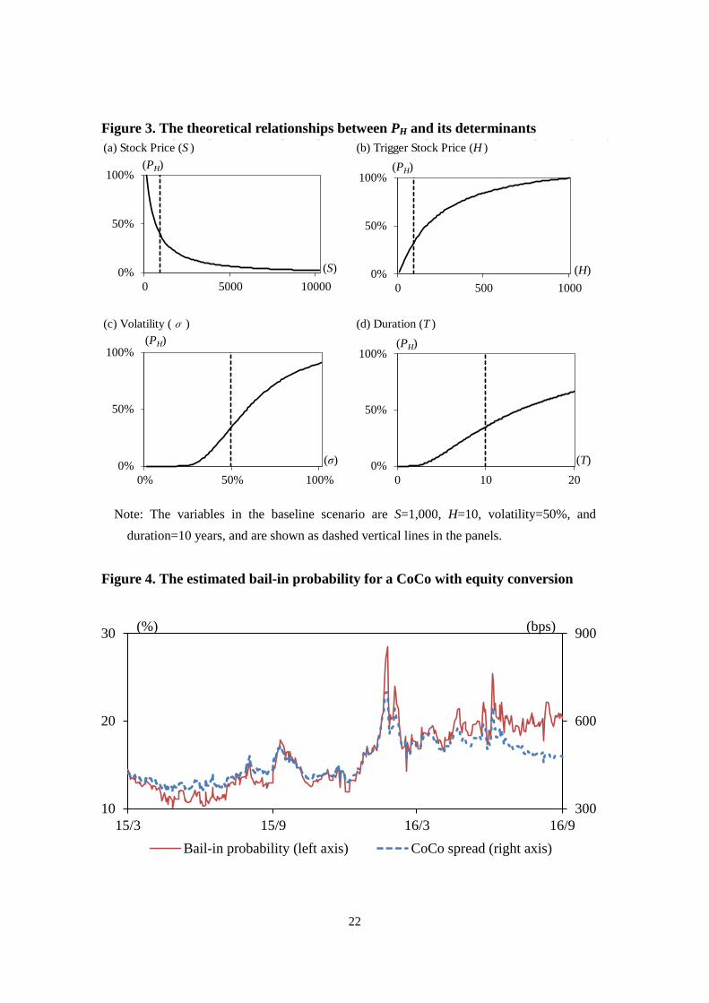
Figure 3. The theoretical relationships between PH and its determinants

Note: The variables in the baseline scenario are S=1,000, H=10, volatility=50%, and

duration=10 years, and are shown as dashed vertical lines in the panels.

Figure 4. The estimated bail-in probability for a CoCo with equity conversion

(a) Stock Price (S ) (b) Trigger Stock Price (H )

(c) Volatility (σ ) (d) Duration (T )

0%

50%

100%

0% 50% 100%

(PH)

(σ)

0%

50%

100%

0 5000 10000

(PH)

(S) 0%

50%

100%

0 500 1000

(PH)

(H)

0%

50%

100%

0 10 20

(PH)

(T)

300

600

900

10

20

30

15/3 15/9 16/3 16/9Bail-in probability (left axis) CoCo spread (right axis)

(%) (bps)

22

Figure 5. Classification of CoCos

Note: In this study, we refer to CoCos with permanent and full write-down as permanent

write-down CoCos.

CoCos

Write-down(WD)

Temporary WD

Permanent WD

Full WD

Partial WD

Equity conversion

W/ fixed conversion price

W/o fixed conversion price

W/ floor price

W/o floor price

23

Figure 6. Probabilities of bail-in and default for European G-SIBs (a) Bank A (b) Bank B

(c) Bank C (d) Bank D

(e) Bank E (f) Bank F

ECB Stress Test

DB Shock

ECB Stress Test DB Shock

ECB Stress Test

DB Shock

ECB Stress Test

DB Shock

24

Figure 7. Conditional probabilities of default after bail-in for selected G-SIBs and their total CoCos issuances in USD

(a) Bank A (b) Bank B

(c) Bank C (d) Bank D

(e) Bank E (f) Bank F

25

Figure 8. Results of the principal components analysis for bail-in probabilities by region

0

20

40

15/09 15/12 16/03 16/06

JapanEurope(including Britain, France, Germany, and Switzerland)China

(%)

26

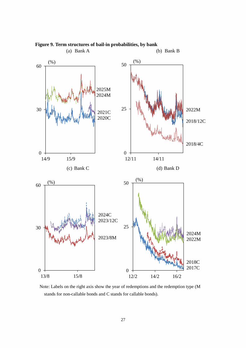
Figure 9. Term structures of bail-in probabilities, by bank (a) Bank A (b) Bank B

(c) Bank C (d) Bank D

Note: Labels on the right axis show the year of redemptions and the redemption type (M stands for non-callable bonds and C stands for callable bonds).

0

30

60

14/9 15/9

2025M 2024M

2021C 2020C

(%)

0

25

50

12/11 14/11

2022M 2018/12C 2018/4C

(%)

0

30

60

13/8 15/8

2024C 2023/12C 2023/8M

(%)

0

25

50

12/2 14/2 16/2

2024M 2022M 2018C 2017C

(%)

27

Figure 10. Bail-in probability and default probability for several maturities for bank D

Figure 11. The implied probabilities of bail-in and default in the short-term (0.1 years) on December 1st, 2016

0

15

30

0 1 2 3 4 5 6 7 8 9 10

CoCo

CDS (Years)

(%)

0.00

0.25

0.50

0 1 2 3 4 5 6 7 8 9 10

P (Bail-in, Dec. 1st, 2015),Max in 4.7YP (Default, Dec. 1st,2015), Max in 10Y

(Years)

(%)

28

Figure 12. Bail-in probabilities for several maturities for bank D before and after the Deutsche Bank shock

Figure 13. Implied probabilities of bail-in in the short-term (0.1 years) for bank D before and after the Deutsche bank shock

0

20

40

0 1 2 3 4 5 6 7 8 9 10

Dec. 1st, 2015

Feb. 10th, 2016

(Years)

(%)

0.00

0.25

0.50

0 1 2 3 4 5 6 7 8 9 10

P (Bail-in, Feb. 10th, 2016),Max in 1YP (Bail-in, Dec. 1st, 2015),Max in 4.7Y

Dec. 1st, 2015 Feb. 10th, 2016

(Years)

(%)

29

Table 1. CoCo issuance by country excluding Japan

Note: As of October 2016. Countries with more than ten issues are listed. Countries outside

Europe are underlined. Source: Bloomberg.

Country # of CoCosBritain 84Norway 37Switzerland 35China 25France 25Ireland 17Denmark 16Sweden 16Germany 15India 15Luxembourg 15Spain 14Brazil 12Netherlands 10

30

Table 2. CoCos issuance by 2016 G-SIBs Bucket Banks CoCo Issuers

4 Citigroup ×

JP Morgan Chase × 3 Bank of America ×

BNP Paribas ○

Deutsche Bank ○

HSBC ○ 2 Barclays ○

Credit Suisse ○

Goldman Sachs ×

Industrial and Commercial Bank of China Limited ○

Mitsubishi UFJ FG ○

Wells Fargo × 1 Agricultural Bank of China ○

Bank of China ○

Bank of New York Mellon ×

China Construction Bank ○

Groupe BPCE ×

Groupe Crédit Agricole ○

ING Bank ○

Mizuho FG ○

Morgan Stanley ×

Nordea ○

Royal Bank of Scotland ○

Santander ○

Société Générale ○

Standard Chartered ○

State Street ×

Sumitomo Mitsui FG ○

UBS ○

Unicredit Group ○ Note: As of November 2016. Source: Bloomberg.

31

Figure A1. Payoff function of temporary write down with variable write-up rate

Assumed Payoff(Write-up Rate)

Stock Price at Maturity

1

0

32