estimating probability of default and · pdf fileestimating probability of default and...

DELOVNI ZVEZKI BANKE SLOVENIJE BANK OF SLOVENIA WORKING PAPERS

1/2014

ESTIMATING PROBABILITY OF DEFAULT AND COMPARING IT TO CREDIT RATING CLASSIFICATION BY BANKS

Matjaž Volk

Izdaja BANKA SLOVENIJE Slovenska 35 1505 Ljubljana telefon: 01/ 47 19 000 fax: 01/ 25 15 516 Zbirko DELOVNI ZVEZKI BANKE SLOVENIJE pripravlja in ureja Analitsko-raziskovalni center Banke Slovenije (telefon: 01/ 47 19 680, fax: 01/ 47 19 726, e-mail: [email protected]). Mnenja in zaključki, objavljeni v prispevkih v tej publikaciji, ne odražajo nujno uradnih stališč Banke Slovenije ali njenih organov. Uporaba in objava podatkov in delov besedila je dovoljena z navedbo vira. CIP - Kataložni zapis o publikaciji Narodna in univerzitetna knjižnica, Ljubljana 336.77:336.711(0.034.2) VOLK, Matjaž Estimating probability of default and comparing it to credit rating classification by banks [Elektronski vir] / Matjaž Volk. - El. knjiga. - Ljubljana : Banka Slovenije, 2014. - (Delovni zvezki Banke Slovenije = Bank of Slovenia working papers, ISSN 2335-3279 ; 2014, 1) Način dostopa (URL): http://www.bsi.si/iskalniki/raziskave.asp?MapaId=1549 ISBN 978-961-6960-00-7 (pdf) 274029824 1. Strojan Kastelec, Andreja 2. Delakorda, Aleš 266187776

ESTIMATING PROBABILITY OF DEFAULT AND COMPARING IT TO CREDIT RATING CLASSIFICATION BY BANKS*

Matjaž Volk†

ABSTRACT Credit risk is the main risk in the banking sector and is as such one of the key issues for financial stability. We estimate various PD models and use them in the application to credit rating classification. Models include firm specific characteristics and macroeconomic or time effects. By linking estimated firms’ PDs with all their relations to banks we find that estimated PDs and credit ratings exhibit quite different measures of firms’ creditworthiness. Results also suggest that in the crisis banks kept riskier borrowers in higher credit grades. This could be due to additional borrower-related information that banks take into consideration in assessing borrowers’ riskiness, to the lags in reclassification process or a possible underestimation of systemic risk factors by banks.

POVZETEK Kreditno tveganje je najpomembnejše izmed tveganj v bančnem sektorju in lahko v primeru realizacije pomembno vpliva na finančno stabilnost. V članku predstavljamo ocene različnih PD modelov ter primerjamo ocenjene verjetnosti neplačila z bonitetnimi ocenami, ki jih banke dodeljujejo posameznim komitentom. Ugotavljamo, da ocenjene verjetnosti neplačila predstavljajo različno mero kreditne sposobnosti podjetij kot bonitetne ocene. Rezultati tudi kažejo, da se je v višjih bonitetnih razredih v času krize poslabšala struktura tveganosti komitentov, merjena z ocenjenimi PD-ji. Razlogi za to so lahko dodatne informacije, na podlagi katerih banke ocenjujejo tveganost komitentov, odlogi pri prerazvrščanju komitentov v nižje bonitetne razrede ali podcenjevanje faktorjev sistemskega tveganja s strani bank. JEL Classification Numbers: G21, G33, C25 Keywords: credit risk, probability of default, credit ratings, probit model * Published in Economic and Business Review, 14 (4). The views expressed in this paper are solely the responsibility of the author and should not be interpreted as reflecting the views of Bank of Slovenia. † Bank of Slovenia (E-mail: [email protected])

Non-technical Summary

Motivated by the growing proportion of firms in overdue we analyze credit risk of Sloveniannon-financial firms. We find that probability of default, which is based on credit overdue, canbe explained with firm specific and macroeconomic or time effects. While firm specific variablesaccount for the cross-section of the default distribution, macroeconomic variables play the role ofshifting the mean of the default distribution in each period. A model that includes year dummiesas time effects performs slightly better than models with macroeconomic variables. This resultis expected, since time dummies might also capture institutional, regulatory or other systematicchanges in time. All models are estimated using random effects probit estimator.

Estimated default probabilities from the two models that best fit the data are compared tocredit rating classification by banks. We link estimated firms’ default probabilities with all theirrelations to banks and analyze credit ratings which represent banks’ assessment of borrowers’creditworthiness. We find that PDs and credit ratings represent quite different measures of creditrisk. Similar is also found if we use credit overdue instead of estimated PDs. The reason for thisis that besides credit overdue banks also consider other factors in classifying debtors into creditgrades. By looking at PD densities for each credit rating we find that in the crisis banks allowfor higher risk borrowers in credit grades A, B and C, which could be due to the underestimationof systemic risk factors in banks’assessment of credit risk.

Netehnični Povzetek

Po izbruhu krize se je delež zamudnikov pri odplačevanju posojila precej povečal, kar jebila poglavitna motivacija za pripravo tega članka, v katerem je analizirano kreditno tveganjeslovenskih nefinančnih družb. Ugotavljamo, da je verjetnost neplačila, ki temelji na zamudahkomitentov pri odplačevanju posojila, odvisna od učinkov, ki so značilni za posamezno podjetje inmakroekonomskih oz. časovnih učinkov. Medtem ko mikroekonomske spremenljivke diferencirajokomitente glede na njihovo kreditno sposobnost, časovni vplivi delujejo na vsa podjetja v enakimeri in s tem določajo povprečno verjetnost neplačila. Izmed časovnih učinkov imajo največjopojasnjevalno moč časovne neprave spremenljivke, ki poleg makroekonomskih nihanj zajamejotudi institucionalne, regulatorne in druge sistemske spremembe v času. Vsi modeli so ocenjeni spanelnim modelom slučajnih učinkov.

Pri analizi razvrščanja komitentov v bonitetne razrede so uporabljene ocenjene verjetnostineplačila iz dveh modelov, ki imata največjo pojasnjevalno moč. Komitentu je pri vsaki banki,do katere ima obveznost, pripisana njegova ocenjena verjetnost neplačila. S tem določen komitentdo vseh bank predstavlja enako tveganje neizpolnitve obveznosti. Rezultati kažejo, da bonitetneocene in ocenjene verjetnosti neplačila predstavljajo dokaj različne mere kreditnega tveganja.Podobno velja tudi za primerjavo bonitetnih ocen in zamud pri odplačevanju posojila. Razlog zato je, da banke pri razvrščanju komitentov v bonitetne razrede poleg zamud upoštevajo tudi drugedejavnike. S proučevanjem gostote verjetnosti neplačila za vsako bonitetno oceno ugotavljamo,da se je bankam v krizi poslabšala struktura tveganosti komitentov, merjena z ocenjenimi PD-ji, v bonitetnih razredih A, B in C. Ocenjujemo, da na to lahko vpliva predvsem premajhnoupoštevanje sistemskih dejavnikov v bančnih ocenah kreditnega tveganja.

5

1. Introduction

After the start of the crisis in 2007 credit risk has become one of the main issues for analystsand researchers. The deteriorated financial and macroeconomic situation forced many firms intobankruptcy or to a significantly constrained business activity. Banks were to a large extentunprepared to such a large shock in economic activity so they suffered huge credit losses in thefollowing years. Although it is clear that credit risk increases in economic downturn, this effectmight be amplified when banks ex-ante overestimate the creditworthiness of borrowers. Underconditions of fierce competition and especially in periods of high credit growth banks mightindeed be willing to assign higher credit ratings to obligors, which could cause problems in theirportfolios when economic situation worsens.

Knowing why do some firms default while others don’t and what are the main factors thatdrive credit risk is very important for financial stability. Since the pioneering work of Altman(1968), who uses discriminant analysis technique to model credit risk, a large set of studiesfind that credit risk is in general driven by idiosyncratic and systemic factors (Bangia et al.,2002; Bonfim, 2009; Carling et al., 2007 and Jiménez & Saurina, 2004). The importance ofmacroeconomic effects is to capture counter-cyclicality and correlation of default probabilities.On the other hand there is also a strong reverse effect of credit risk on macroeconomic activity.Gilchrist and Zakrajšek (2012) find that a level of credit risk statistically significantly explainsthe movement of economic activity. They construct a credit spread index (GZ spread) whichindicates high counter-cyclicality movement and has high predictive power for variety of economicindicators.

This paper analyses credit risk of Slovenian non-financial firms using an indicator of firmdefault based on credit overdue. We focus on modelling default probability and use similarapproach as those proposed by Bonfim (2009) and Carling et al. (2007). The results obtainedsuggests that probability of default (PD) can be explained by firm specific characteristics aswell as macroeconomic or time effects. While macro variables influence all firms equally, andthus drive average default probability, firm specific variables are crucial to distinguish betweenfirms’ creditworthiness. Similar as Bonfim (2009), we find a model that includes time dummiesas time effects to perform slightly better than model with macroeconomic variables. This resultis expected, since time dummies also capture institutional, regulatory or other systemic changesin time. The main contribution of this paper is that we compare the estimated PDs to creditrating classification by banks. We select two models that best fit the data and link the estimatedfirm-level PDs with all credit grades which are given to borrowers by banks. We find thatestimated PDs and credit ratings by banks often exhibit quite different measures of credit risk.The results also suggest that in the crisis banks allow for higher risk borrowers in credit gradesA, B and C. This could be due to additional borrower-related information that banks take intoconsideration in assessing borrowers’ riskiness, to the lags in reclassification process or a possibleunderestimation of systemic risk factors by banks.

The rest of the paper is structured as follows. Next section presents the data. Section3 describes the modelling approach used to estimate the probability of default. Estimationresults of various credit risk models and an application of the models in analysis of credit ratingclassification is presented in Section 4. Section 5 concludes the paper.

2. Data

Three different data sources are combined to construct dataset used in the econometric anal-ysis. First, balance sheet and income statement data for all Slovenian firms are collected by theAgency of the Republic of Slovenia for Public Legal Records and Related Services (AJPES) at

6

yearly basis. The analysis is restricted only to non-financial corporations. Second, data aboutcredit exposures, credit ratings, credit overdue, etc. are gathered in Credit register at Bank ofSlovenia. The banks are mandatory to report these data every month, but since firms’ balancesheet and income statement data are only available at yearly basis, we use the end-of-year data.Third, to capture the business cycle effects when modelling PD, we use a set of macroeconomicand financial series which are obtained from Statistical Office of the Republic of Slovenia (SURS)and from Bank of Slovenia.

Two different subsets of the data are used for modelling probability of default and in com-parison of the estimated PDs to credit rating classification by banks. Hence we present each ofthem separately.

2.1. Data for Modelling PDUnder the framework of Basel II the obligor defaults on his credit obligation if (1) he is

unlikely to pay the obligation or (2) is passed overdue more than 90 days (BCBS, 2006). Sinceit is difficult to set the objective criteria for unlikeliness of paying the obligation, we derive theindicator of firm default from credit overdue. Firm i is in default if its principal or interestpayments are more than 90 days overdue in at least one bank in year t. The stock of defaultedfirms increased significantly in the crisis, from 3.9% in 2007 to 9.9% in 2010.

To model the PD we use yearly data from 2007 to 2010. Since PD is the probability that afirm will default in year t given that it did not default in year t − 1, all firms who have for thefirst time taken the loan (in any bank) in year t are excluded form the sample. Firms that werein the state of default for two or more consecutive years are also excluded and only their firstmigration to the state of default is taken into account. Similar to Bonfim (2009), we keep all thefirms that defaulted twice or more in a given sample, but not in two consecutive years.

The firm’s financial ratios like measures of liquidity, solvency, indebtedness, cash flow, prof-itability, etc. are key inputs to PD models. They capture firm specific effects and reflect theriskiness of firms. The sample additionally excludes firms with significant outlier in some of theircharacteristics so that all the observations in the 1st and the 100th percentile are dropped. Table1 presents the summary statistics for some financial ratios and the other firm’s characteristics fordefaulted and non-defaulted firms, which are taken into account in the analysis, for the period2007-2010. We now turn to the descriptive analysis of the variables.

Total sales which is a measure of firm size indicates that defaulted firms are on averagesmaller. Similar result is found by other researchers like Antão and Lacerda (2011), Carling etal. (2007), Kavčič (2005) and Psillaki et al. (2010). Smaller firms are less diversified and rely onless or perhaps on a single project. They are often also more financially constrained comparingto larger firms and may have problems in raising funds in economic downturns (Bernanke et al.,1996, 1999).

Defaulted firms are on average younger, have lower liquidity, higher leverage, lower cashflow, worse operating performance and have lower interest coverage, comparing to non-defaultedfirms. A significantly useful indicator to separate between firms in default and non-default isalso a variable which measures a number of days a firm has blocked bank account per year. Itshows that in a given sample defaulted firms’ bank accounts were on average blocked 106 daysper year, whereas accounts for firms with no default were on average blocked only 6 days peryear.

Somewhat less expectedly firms in default have on average higher amount of total credit.Jiménez and Saurina (2004) indeed show that there is an inverse relationship between the sizeof the loan and the probability of default since larger loans are more carefully screened. Thedifference between the two approaches is that their research is done at loan level, whereas thisanalysis is at firm level, where the default occurs if a firm defaults in any bank in year t.

7

Table 1: Summary Statistics for Firms With and Without Defaults

Firms with no default Firms in defaultMean St. dev. Mean St. dev.

Total sales (EUR million) 2.2 13.5 1.1 3.7Firm age (in years) 13.4 6.6 12.0 6.7Quick ratio 1.3 1.6 0.9 1.1Debt-to-assets 0.7 0.3 0.9 0.5Cash flow 0.1 0.2 -0.1 0.5Asset turnover ratio 1.5 1.9 0.8 1.0Interest coverage 4.6 11.2 -0.3 7.3Blocked account (in days) 5.9 32.6 105.8 127.5Total credit (EUR million) 0.4 1.1 0.7 1.4No. of bank-borrower relationships 1.4 0.7 1.8 1.0

No. of observations 65557 2887

Source: Bank of Slovenia, AJPES, own calculations.Notes: The table reports the summary statistics for firms’ financial ratios and other variablesused for PD modelling. It is calculated for the period 2007-2010. Statistics for Interest cov-erage are computed on reduced sample of 45236 observations due to the missing values.

According to the relationship banking theory banks and borrowers can benefit from a closerelationship (Boot, 2000). Especially small banks tend to have comparative advantage in usingsoft information technologies (Berger & Udell, 2002). Nevertheless, in a recent study, Bergerand Black (2011) show that bank will generally choose a hard information technology over a softinformation technology if a sufficient hard information is available. The results of Jiménez andSaurina (2004) indicate that when borrower’s loans are spread across several banks there is lessof an incentive to finance riskier borrowers. Banks are willing to finance higher risk borrowers ifthey have a close relationship with them. This seems not to hold in the case of Slovenia sincefirms in default have on average higher number of bank-borrower relationships. One explanationmight be that risky firms seek for credit in other banks because current creditors don’t want tolend them any more if they are not paying off the loan regularly. The borrower’s credit historyis in general not available to new creditors, thus they can only assess firms’ creditworthinessthrough their financial ratios.

Jacobson et al. (2011) argue that firm-specific variables account for the cross-section of thedefault distribution, while macroeconomic variables play the role of shifting the mean of thedefault distribution in each period. Finally, care is taken to include business cycle effects in themodel. Figure 1 illustrates the movement of default rate for a given sample against the twoindicators of the business cycle. The default rate appears to be highly countercyclical and itseems more tightly related to credit growth than to GDP growth. As shown by Bonfim (2009),Jiménez and Saurina (2006) and others, most of the credit risk is built up during periods ofstrong credit growth when banks apply looser credit standards. This risk materializes whenthe economy hits a downturn. With looser credit standards banks attract more risky borrowerswhich deteriorate their average assets quality. Marcucci and Quagliariello (2009) find that bankswith lower asset quality are much more vulnerable in recessions. The increase in default ratesdue to one percentage point decrease in output gap is almost four times higher for those banksthan the effect on banks with better portfolios.

8

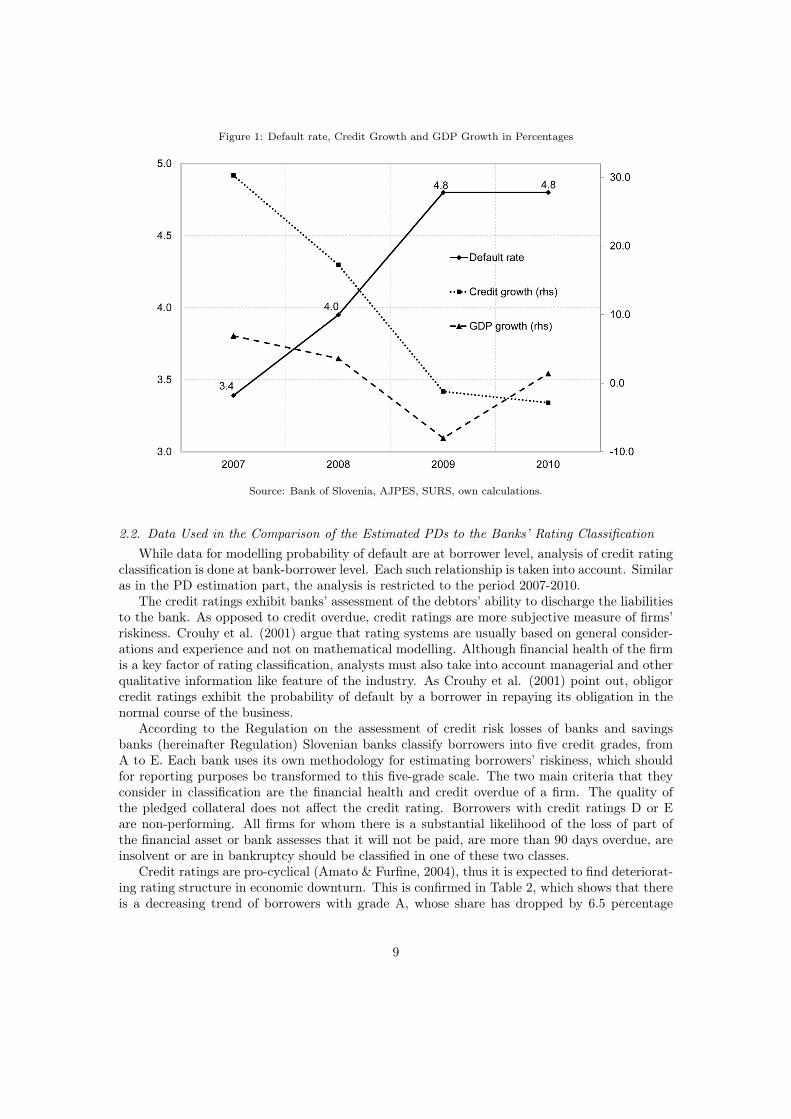
Figure 1: Default rate, Credit Growth and GDP Growth in Percentages

Source: Bank of Slovenia, AJPES, SURS, own calculations.

2.2. Data Used in the Comparison of the Estimated PDs to the Banks’ Rating ClassificationWhile data for modelling probability of default are at borrower level, analysis of credit rating

classification is done at bank-borrower level. Each such relationship is taken into account. Similaras in the PD estimation part, the analysis is restricted to the period 2007-2010.

The credit ratings exhibit banks’ assessment of the debtors’ ability to discharge the liabilitiesto the bank. As opposed to credit overdue, credit ratings are more subjective measure of firms’riskiness. Crouhy et al. (2001) argue that rating systems are usually based on general consider-ations and experience and not on mathematical modelling. Although financial health of the firmis a key factor of rating classification, analysts must also take into account managerial and otherqualitative information like feature of the industry. As Crouhy et al. (2001) point out, obligorcredit ratings exhibit the probability of default by a borrower in repaying its obligation in thenormal course of the business.

According to the Regulation on the assessment of credit risk losses of banks and savingsbanks (hereinafter Regulation) Slovenian banks classify borrowers into five credit grades, fromA to E. Each bank uses its own methodology for estimating borrowers’ riskiness, which shouldfor reporting purposes be transformed to this five-grade scale. The two main criteria that theyconsider in classification are the financial health and credit overdue of a firm. The quality ofthe pledged collateral does not affect the credit rating. Borrowers with credit ratings D or Eare non-performing. All firms for whom there is a substantial likelihood of the loss of part ofthe financial asset or bank assesses that it will not be paid, are more than 90 days overdue, areinsolvent or are in bankruptcy should be classified in one of these two classes.

Credit ratings are pro-cyclical (Amato & Furfine, 2004), thus it is expected to find deteriorat-ing rating structure in economic downturn. This is confirmed in Table 2, which shows that thereis a decreasing trend of borrowers with grade A, whose share has dropped by 6.5 percentage

9

points since 2008, whereas the share of non-performing firms has increased by two thirds. Asimilar shift is also noted from credit overdue in Table 3, where the share of borrowers who aremore than 90 days overdue increased by 3 percentage points since its lowest value in 2007. Thusthe proportion of firms who are more than 90 days overdue is much lower on bank-borrowerlevel than on firm level, where this proportion increased by 6 percentage points (2.5-times) inthe same period. Once a firm is in overdue in one bank, there is a substantial likelihood thatin the following periods it becomes a delinquent also in other banks to which it has liabilities.Especially in economic downturns when firms struggle to repay the debt, significantly increasedcredit overdue in one bank clearly indicates that the firm has financial problems and thus exhibitsa higher credit risk to all banks to which it has liabilities.

Table 2: Credit Rating Structure in Percentages

Credit rating 2007 2008 2009 2010A 57.3 57.9 53.7 51.4B 32.7 31.7 33.0 33.9C 5.2 6.1 7.5 7.5D 3.4 3.2 4.4 4.6E 1.3 1.2 1.5 2.5No. of bank-borrowerrelationships 28318 29876 30633 31524

Source: Bank of Slovenia, own calculations.

Table 3: Percentages of Firms in Overdue

Credit overdue 2007 2008 2009 20100 days 93.1 90.9 89.3 88.11-90 days 3.4 5.0 5.1 5.4more than 90 days 3.4 4.1 5.6 6.5No. of bank-borrowerrelationships 27118 28598 29472 30447

Source: Bank of Slovenia, own calculations.Note: All the observations with no data for credit overdue are excluded.

Table 4 shows the distribution of firms according to their credit rating and credit overduein particular bank in the period 2007-2010. It shows that these two measures exhibit a quitedifferent assessment of firms’ riskiness. Although according to the Regulation credit grade Dshould include borrowers that are in relatively bad condition or are more than 90 days overdue,around 50% of D borrowers is repaying its obligations without overdue. On the other hand,among borrowers who are more than 90 days overdue, around 5% are classified as A borrowersand 38% are classified in grades A, B or C.

Banks probably use also internal soft information in determining firms’ credit rating. Creditoverdue is not the only measure for classifying borrowers into credit grades. Close relationshipwith firms can provide a more detailed information which can not be inferred from firms’ financialaccounts but adds valuable information in assessing firms’ creditworthiness. For this reasoncredit overdue and credit ratings exhibit quite different risk structure. However, the proportionof borrowers with more than 90 days overdue in high credit grades still seems quite high.

Table 5 displays credit rating transitions which are computed on one-year horizons. In 2009when macroeconomic conditions deteriorated significantly, banks downgraded larger share of

10

Table 4: Credit Ratings versus Credit Overdue in the Period 2007-2010

Overdue Credit Ratingin days A B C D E Total

Frequency 60200 35767 5786 2372 284 1044090 Row percentage 57.7 34.3 5.5 2.3 0.3 100.0

Column percentage 96.9 91.6 73.6 50.8 14.6 90.3

Frequency 1667 2498 914 368 44 54911-90 Row percentage 30.4 45.5 16.7 6.7 0.8 100.0


Frequency 261 768 1159 1928 1619 5735>90 Row percentage 4.6 13.4 20.2 33.6 28.2 100.0


Frequency 62128 39033 7859 4668 1947 115635Total Row percentage 53.7 33.8 6.8 4.0 1.7 100.0


Source: Bank of Slovenia, own calculations.Note: The table reports the distribution of firms according to their credit rating and credit overdue in the2007-2010 period.

borrowers than in the pre-crises period. Comparing to 2009 only downgrades from credit gradesC and D increased in 2010, whereas those form A and B decreased. There was also largerproportion of credit rating improvements in 2010. Despite the first signs of slowdown in thesecond half of 2008, banks upgraded higher proportion of borrowers in 2008 than a year beforewhen GDP grew substantially. In the following sections we check what would be the change inrating structure according to the model-estimated PDs.

Table 5: Proportions of Increases, Decreases and No-changes of Credit Ratings in Percentages

Rating increased Rating did not change Rating decreased2007 2008 2009 2010 2007 2008 2009 2010 2007 2008 2009 2010

A 89.9 91.4 87.1 87.6 10.1 8.6 12.9 12.4B 9.6 10.1 3.8 7.3 83.0 79.2 81.9 81.2 7.5 10.8 14.3 11.6C 21.0 21.7 11.0 15.9 68.2 65.7 71.1 63.8 10.8 12.6 17.9 20.3D 16.5 22.8 10.8 10.1 78.7 69.6 79.2 62.5 4.8 7.6 9.9 27.5E 8.5 12.1 2.9 3.6 91.5 87.9 97.1 96.4

Source: Bank of Slovenia, own calculations.Note: The table reports the percentages of credit rating transitions, calculated on one-year horizons.

3. Empirical Model

Credit losses are typically measured with expected loss, which is a product of probabilityof default, loss given default and exposure at default (EL = PD ∗ LGD ∗ EAD). While PDis counter-cyclical, recovery rates are usually pro-cyclical since the value of collateral falls ineconomic downturn. Bruche and González-Aguado (2010) find that macroeconomic variablesare in general significant determinants of default probabilities but not so for recovery rates.

11

They show that although the variation in recovery rate distributions over time has an impacton systemic risk, this impact is small relative to the importance of the variation in defaultprobabilities. Hence, we focus on modelling PD, which also enable us to compare estimated PDswith credit rating classification by banks.

Many different approaches for modelling default probability are proposed in the literature.Altman (1968) proposes a model which relies on firm-specific variables, like asset turnover ratio,EBIT/total assets, working capital/total assets, etc. With some modifications this approach iswidely used nowadays. Instead of discriminant analysis modelling technique researchers now uselogit or probit models. Since the defaults are correlated, aggregate time varying factors (likeGDP growth, unemployment rate, etc.) have to be included in the models. These factors arecommon to all obligors and drive their credit risk into the same direction. In this respect wefollow previous work by Bangia et al. (2002), Bonfim (2009), Carling et al. (2007), Jiménezand Saurina (2004) and others. Some authors, such as Festić et al. (2011), Foss et al. (2010)and Jiménez and Saurina (2006) stress another important aspect of macro effects on credit risk,arguing that strong GDP or credit growth before the crisis may have increased the share ofdefaulted firms or deteriorate NPL dynamics. The reason for this is that banks apply loosercredit standards in expansions and thus attract more risky borrowers, which shows up duringrecessions when default rates rise.

Merton (1974) introduces a structural credit risk model where defaults are endogenouslygenerated within the model. It is assumed that the default happens if the value of assets fallsshort of the value of liabilities. One of the model’s major drawbacks is the availability of marketprices for the asset value. Such data are usually not available for small and medium sizedenterprises. As shown by Hamerle et al. (2003), Hamerle et al. (2004) and Rösch (2003) it ispossible to overcome this problem with latent variable approach. They model the default eventas a random variable Yit which takes value 1 if firm i defaults in time t and 0 otherwise. Thedefault event happens when borrower’s return on assets, Rit, falls short of some threshold cit.The probability that a firm i will default in time t, given the survival until time t−1 is describedby the threshold model:

λit = P (Rit < cit | Rit−1 ≥ cit−1) (1)

Equivalently this probability can be described with discrete time hazard rate model whichgives the probability that firm i defaults in time t under the condition that it did not defaultbefore time t:

λit = P (Ti = t | Ti > t− 1) (2)

As discussed by Hamerle et al. (2003) it can always be assumed that the default event, Yit, isobservable. On the other hand the observability of the return on firm’s assets, Rit, depends onthe available data. If Rit is observable then the model is linear. Otherwise a nonlinear model,such as logit or probit, is estimated, which treats the return on assets as a latent variable.

We estimate the probability that firm i defaults in year t given that it did not default inprevious year P (Ti = t | Ti > t− 1) using different specifications of the model:

P (Yit = 1 | Xit, Zt) = F (α+ βXit + γZt) (3)

where Yit is a binary variable which takes value 1 if firm i defaults in time t and 0 otherwise, α isconstant term, Xit is a vector of firm specific variables including also time invariant factors likesectoral dummies and Zt is a vector of time varying explanatory variables, such as time dummiesand macroeconomic effects. F (·) is cumulative distribution function which is standard normal

12

distribution function Φ(·) in the case of probit model and logistic distribution function Λ(·) inthe case of logit model.

The estimated PDs are used in comparison to credit rating classification by banks. Bankscan observe firms’ riskiness in time t through monitoring process and can also observe the stateof the economy. Moreover, the main criterion that banks consider in classifying borrowers incredit grades is credit overdue, which is available to banks regularly in time t. This means thatin time t banks have a large set of information to decide about firms’ creditworthiness. To ensurethat we are using the same set of information as available to banks in time t we include all thevariables in the model at their values in time t, with few exceptions.

To estimate P (Yit = 1 | Xit, Zt) we apply random effects probit model. This estimator is mostoften used in other research and is the underlying model in Basel II risk assessment procedures.Hamerle et al. (2003) show that when only defaults are observable, an appropriate thresholdmodel leads to random effects probit or logit model.

We use the measures of goodness of fit described by BCBS (2005) and Medema et al. (2009).The most often used method for determining the discrimination power of binary models is Re-ceiver Operating Characteristics (ROC) curve. It is obtained by plotting hit rate (HR) againstfalse alarm rate (FAR) for different cut-off points. HR is percentage of defaulters that are cor-rectly classified as defaulters and FAR is percentage of non-defaulters incorrectly classified asdefaulters. The area under this curve indicates that the model is noninformative if it is close to0.5 and the closer it is to 1, the better the discriminating power of the model.

The Brier Score is defined as BS = 1N

∑Ni=1(P̂Di − Yi)2 where P̂Di is estimated probability

of default. As explained by Medema et al. (2009) it can be interpreted as the mean of the sumof squares of the residuals. The better the model, the closer BS is to zero.

Finally, pseudo R2 is based on log-likelihood values of estimated model (L1) and a modelwhich contains only constant as explanatory variable (L0): Pseudo R2 = 1− 1

1+2(logL1−logL0)/N.

We also use Likelihood Ratio (LR) test which enables to compare two models of which one isnested into the other. It is defined as LR = 2[logL(θ̂) − logL(θ̃)], where logL(θ̂) and logL(θ̃)are log-likelihoods of unrestricted and restricted models, respectively.

4. Results

In the first part of this section, we present the estimation results of different credit risk modelspecifications. Estimated PDs from the two model specifications that best fit the data are thenused in the second part in the comparison of estimated PDs to credit rating classification bybanks. In the third part we check the robustness of the obtained results by excluding a variablethat measures number of days a firm has blocked bank account from the model.

4.1. Estimation ResultsTable 6 shows the results of random effects probit models with various firm specific variables,

sector dummies and time effects. In all the estimates, robust standard errors are used.The basic model is given in first column of Table 6. It includes only firm specific variables.

All coefficients are different from zero at 1% probability and display the expected sign. Totalsales displays a negative coefficient, suggesting that larger firms have lower probability of default.Size of a firm is in many researches found as one of the most important ingredients of credit riskmodels, since smaller firms are in principle less diversified, have lower net worth and are morefinancially constrained. Similar result is also found for firm age, which indicates that youngerfirms who are usually more sensitive to shocks default more often.

Quick ratio, which is an indicator of liquidity, measures the ability of firm to use its quickassets (current assets minus inventories) to meet its current liabilities. As expected, firms with

13

Table 6: Estimated PD Models

(1) (2) (3) (4) (5) (6) (7)Est. Method RE Probit RE Probit RE Probit RE Probit RE Probit RE Probit RE Probit

Firm variables

Total sales -0.017*** -0.019*** -0.018*** -0.018*** -0.018*** -0.018*** -0.019***Firm age -0.014*** -0.013*** -0.014*** -0.013*** -0.014*** -0.013*** -0.013***Quick ratio -0.042*** -0.036*** -0.041*** -0.036*** -0.035*** -0.034*** -0.036***Debt-to-assets 0.540*** 0.560*** 0.540*** 0.554*** 0.542*** 0.547*** 0.559***Cash flow -0.138*** -0.137*** -0.137*** -0.135*** -0.138*** -0.140*** -0.136***Asset turnover r. -0.268*** -0.278*** -0.270*** -0.274*** -0.271*** -0.274*** -0.277***Blocked account 0.007*** 0.008*** 0.007*** 0.008*** 0.007*** 0.008*** 0.008***No. of bank-borr. r. 0.363*** 0.379*** 0.369*** 0.375*** 0.368*** 0.371*** 0.378***

Sectoral dummies

Agric., Forestry, 0.070 0.067 0.068 0.067 0.063 0.068Fish. and MiningElectricity, gas -0.404*** -0.391*** -0.395*** -0.391*** -0.393*** -0.399***and water supplyConstruction -0.001 -0.000 -0.001 -0.000 0.002 -0.000Commerce -0.045 -0.045 -0.045 -0.045 -0.043 -0.044Tran. and storage 0.071 0.068 0.071 0.067 0.070 0.072Accomodation 0.168*** 0.156*** 0.166*** 0.157*** 0.161*** 0.169***and food serviceInf. and commun. -0.246*** -0.241*** -0.246*** -0.238*** -0.241*** -0.248***Fin. and insur. -0.304* -0.301* -0.299* -0.303* -0.298* -0.298*Real estate 0.087 0.077 0.084 0.080 0.083 0.086Professional act. -0.169*** -0.164*** -0.168*** -0.164*** -0.164*** -0.169***Public services -0.206*** -0.201*** -0.203*** -0.198*** -0.201*** -0.206***

Time effects

2008 0.212***2009 0.173***2010 0.209***GDP growth -0.011***GDP growth (t-1) -0.038***NFC loan growth -0.005*** -0.007***NFC loan g. (t-1) 0.018***Interest rate 0.024*** 0.046***Quick r.*GDP g. 0.006*** -0.001

Constant -2.426*** -2.635*** -2.403*** -2.414*** -2.401*** -2.654*** -2.381***Observations 68444 68444 68444 68444 68444 68444 68444Pseudo R2 0.094 0.096 0.095 0.095 0.095 0.095 0.096Log. lik. -8382.7 -8313.6 -8331.2 -8326.7 -8332.5 -8328.9 -8321.1LR test - 138.4 103.1 112.1 100.4 107.6 123.3AUC 0.888 0.890 0.889 0.889 0.890 0.890 0.889Brier score 0.030 0.029 0.030 0.029 0.030 0.030 0.029

Source: Bank of Slovenia, AJPES, SURS, own calculations.* p < 0.10, ** p < 0.05, *** p < 0.01; Robust standard errors are used.Notes: The table reports the estimated probit models for the period 2007-2010, where the dependent variable isthe indicator for firm’s default, based on credit overdue. Blocked account is a number of days a firm has blockedbank account, No. of bank-borr. r. measures to how many banks a particular firm is related to. GDP growth isin real terms. NFC credit growth is real growth of loans to non-financial corporations, Interest rate is long-terminterest rate on loans to non-financial corporations, AUC is area under ROC curve.

14

higher liquidity ratios have lower default probabilities. Defaulted firms are generally expected tohave more debt in their capital structure. The positive sign on the coefficient for debt-to-assetsratio in the model clearly indicates that firms with higher leverage default more often. Cashflow, which is a ratio between operating cash flow and revenues, displays a negative coefficient.It is expected that stable, mature and profitable firms generate sufficient cash flows to payoff the owners and creditors. Asset turnover ratio measures firm’s efficiency in generating salesrevenues with assets. The estimated coefficient indicates that firms that are more efficient defaultless often. Number of days a firm has blocked bank account also seems to offer an importantcontribution in explaining firm’s credit default. The longer the firms have blocked bank accountin a given year, the higher the probability of default.

Number of bank-borrower relationships displays highly statistically significant coefficient withpositive sign, which is contrary to the findings of Jiménez and Saurina (2004) and indicates thatthose firms with more credit relationships have on average higher default probability. This resultsuggests that less creditworthy firms seek for credit in more banks, possibly because currentcreditors don’t want to lend them any more or are only prepared to grant smaller amount ofcredit due to their riskiness.

We now extend the model with aggregate variables, i.e. the sectoral and time dummies.Many authors like Antão and Lacerda (2011) and Crouhy et al. (2001) suggest taking intoaccount the features of the industry when modelling credit risk. In our sample defaulters andnon-defaulters are similarly distributed across sectors, with the highest representativeness ofCommerce (28%), Manufacturing (18%), Professional activities (17%) and Construction (11%).By including sectoral dummies in model (2), the dummy variable for manufacturing firms isomitted, so that the coefficients for other sectors indicate the relative riskiness of a particularsector in relation to manufacturing one. Year dummies (omitting the dummy variable for 2007)are capturing the time effects. It is wider category than macroeconomic variables, which willbe added in further specifications, since it also captures institutional, regulatory or any othersystemic factors that affect all firms. Although some of the sectoral dummies are insignificant,it is clear that there are some differences in credit risk across sectors. Sectors like electricity,gas and water supply, information and communication, professional activities and public servicesare less risky than manufacturing, whereas only accommodation and food service has on averagehigher statistically significant default probability. By adding both sectoral and time dummiescoefficients of firm specific variables are changed only slightly, which indicates that these two setof aggregate variables are close to independent from firm specific effects. According to likelihoodratio test, sector and time dummies improve the fit considerably comparing to model (1).

Since the default rate is highly related to the business cycle - increasing in economic downturns- a set of macroeconomic and financial variables is included in models (3) to (7). GDP growth asthe main indicator of economic activity is added in model (3). The estimated coefficient suggeststhat higher economic activity lowers the probability of default, because better macroeconomicsituation enables a better performance of all firms. The only significant interaction effect betweenGDP growth and firm specific variables is the one with the quick ratio, which shows how theeffect of liquidity changes with one percentage point increase in GDP growth and vice versa.Similar result is also found in model (4) where growth of credit to non-financial corporationsis used as an alternative indicator of the business cycle. According to the likelihood ratio test,credit growth actually seems to be more a powerful business cycle variable for explaining defaultprobability than GDP growth. The interest rate on bank loans is also expected to have animportant influence on the borrowers’ ability to repay loans. As suggested by the coefficient oninterest rate in model (5), a higher interest rate leads to a higher probability of default, whichalso make sense, since it increases borrowers’ credit burden.

Among macroeconomic variables, the credit growth seems to have the highest explanatory

15

power in terms of default probabilities. When credit growth and interest rates are put together,as in model (7), it further improves the fit as can be seen from the likelihood ratio test statistic.We also estimate models with different combinations of business cycle indicators, but many ofthem were found insignificant or with unexpected sign. Short time series does not allow us toinclude many variables that vary in time and are constant for all firms.

Model (6) includes GDP and credit growth lagged one year. Lagged GDP growth exertsa negative effect on probability of default, as in contemporaneous case, although the displayedcoefficient is now higher in absolute terms. On the other hand, lagged credit growth displays apositive coefficient, which suggests that high past credit growth increases probability of default,as expected. When economic situation turns around, as it did in 2009-2010, and risk premiumstarts rising due to the tightening credit standards, these borrowers quickly get into trouble andmay default on their credit obligations.

4.2. The Comparison of Estimated PDs to Credit Rating Classification by BanksAs the estimated PD exhibit a measure of risk conditional on a large set of available informa-

tion, it is interesting to compare it to the credit ratings by banks. Credit ratings indeed exhibitthe banks’ assessment of debtors’ ability to repay the debt. For the purpose of comparison, welink firms’ probabilities of default with all credit ratings by banks. Since PDs are estimated atfirm level, a particular firm represents the same level of risk to all banks that have exposure tothis firm.

To select the model specification for this analysis we use root-mean-square error, which is

defined as RMSE =√

1T

∑Tt=1(DRPt −DRAt)2, where DRPt and DRAt are predicted and

actual default rate in time t, respectively. Table 7 shows that the in-sample predicted defaultrate from model (2), which includes year dummies as time effects, is the most unbiased. Thisresult might be expected since time dummies do not only capture the macroeconomic dynamicsbut also other institutional, systemic or regulatory changes. Among models with macroeconomicvariables, model (7), which includes credit growth and interest rate as business cycle effects,is the most accurate. Since these two models give the most unbiased in-sample predictions forthe default rate and have high overall classification accuracy rate (96.3%) we use them in thecomparison to the banks’ risk grades.

Table 7: Actual vs. In-Sample Predicted Default Rate

2007 2008 2009 2010 RMSEActual default rate 3.39 3.95 4.80 4.80

In-sample predicted default rateModel 1 4.07 3.56 4.58 4.36 0.46Model 2 3.38 3.92 4.71 4.67 0.08Model 3 3.89 3.46 4.94 4.31 0.43Model 4 3.66 3.40 4.90 4.68 0.32Model 5 3.80 3.65 4.98 4.18 0.41Model 6 3.80 3.82 4.29 4.73 0.34Model 7 3.58 3.57 4.59 4.92 0.24

Source: Bank of Slovenia, AJPES, SURS, own calculations.Note: In-sample predicted default rate is calculated as average of firms’ PDs.

Table 8 shows the distribution of firms according to their credit ratings and the level ofestimated PD in the period 2007-2010. In all credit grades, except E, the majority of firms have

16

PD between 1 and 5 percent. Although we would expect borrowers in credit grade D to havehigh PDs on average, 43% have PD below 5%. Among high-risk borrowers with PD above 50%,around 13% are classified as A borrowers and approximately 57% are classified in grades A, Bor C. This results are similar as those in Table 4 where instead of PD, the distribution is doneaccording to credit overdue.

Table 8: The Distribution of Firms Among PD Buckets and Credit Grades

Credit RatingPD A B C D E Total

Model 2PD ≤ 1 18641 7596 868 399 16 275901 < PD ≤ 5 24621 15815 2296 808 57 435975 < PD ≤ 10 5669 4727 1062 406 58 1192210 < PD ≤ 25 2992 2944 933 383 63 731525 < PD ≤ 50 748 838 395 285 68 2334PD > 50 202 368 334 504 178 1586

Model 7PD ≤ 1 18519 7488 855 396 13 272711 < PD ≤ 5 24776 15899 2317 815 62 438695 < PD ≤ 10 5711 4784 1070 386 53 1200410 < PD ≤ 25 2949 2938 924 398 66 727525 < PD ≤ 50 710 795 398 280 70 2253PD > 50 208 384 324 510 176 1602Total 52873 32288 5888 2785 440 94274

Source: Bank of Slovenia, AJPES, SURS, own calculations.Note: The table reports the number of firms distributed among PD buckets and creditgrades for 2007-2010 period.

Estimated PDs allow us to test whether banks’ rating criteria were constant in time. If banksuse unique criteria to assess borrowers riskiness, the risk structure in terms of PDs of firms ineach credit grade should be stable in time. Figure 2, Figure 3 and Table 9 indicate that therisk structure was changing in time, particularly in credit grades A, B and C. This can be bestseen from the changing shapes in distributions of the estimated PDs in different credit grades.This holds for model (2) estimates (Figure 2) as well as for model (7) estimates (Figure 3), withthe largest change in distribution between years 2007 and 2008. In Table 9, average defaultprobability in credit grades A, B and C rose by 1.3, 1.5 and 1.5 percentage point, respectively,as estimated with model (2) and by 0.7, 0.7 and 0.5 percentage point, respectively, as estimatedwith model (7). This trend continued also in 2009 and 2010 where especially for credit grades Aand B model (7) gives more pronounced results. Risk structure deteriorated the most in creditgrade C, where the average default probability estimated with models (2) and (7) increased by4.4 and 4.6 percentage point, respectively, from 2007 to 2010. Somehow surprisingly, in creditgrades D and E the average estimated PD actually decreased in 2008. It is possible that thisresult is driven by small number of borrowers in credit grades D and E.

To get a more clear insight in comparing risk evaluations we check what would be the model-predicted rating structure if banks would keep constant rating criteria in time. To be able to dothis we need to predict credit ratings by setting threshold PDs between each credit grade. Sincethere is a lot of overlapping in default probability between credit ratings, perfect discriminationis not possible. Hence, we set the cut-off PDs so as to ensure that the predicted rating structurein a particular date is equal to actual one. We use as a point of reference first 2007 and then2008. Thus for 2007, we classify the top 56.2% in terms of PDs of firms as A borrowers, next

17

Figure 2: Kernel Densities of PDs Estimated with Model 2, by Credit Rating

0.2

.4.6

Density

0 2 4 6 8 10PD

2007

2008

2009

2010

kernel = epanechnikov, bandwidth = 0.1767

Credit Rating A

0.1

.2.3

.4D

ensity

0 5 10 15PD

2007

2008

2009

2010


Credit Rating B0

.05

.1.1

5.2

Density

0 10 20 30PD

2007

2008

2009

2010


Credit Rating C

0.0

05

.01

.015

.02

.025

Density

0 20 40 60 80 100PD

2007

2008

2009

2010


Credit Ratings D and E


Figure 3: Kernel Densities of PDs Estimated with Model 7, by Credit Rating

0.1

.2.3

.4.5

Density

0 2 4 6 8 10PD

2007

2008

2009

2010


Credit Rating A

0.1

.2.3

.4D

ensity

0 5 10 15PD

2007

2008

2009

2010


Credit Rating B

0.0

5.1

.15

.2D

ensity

0 10 20 30PD

2007

2008

2009

2010


Credit Rating C

0.0

05

.01

.015

.02

.025

Density

0 20 40 60 80 100PD

2007

2008

2009

2010




18

Table 9: Summary Statistics for PDs Estimated with Model 2 and Model 7, by Credit Rating

Model 2 Model 7Mean Std. P50 P90 Skew. Kurt. Mean Std. P50 P90 Skew. Kurt.

Credit Rating A2007 2.6 5.8 1.1 5.8 7.8 91.1 2.8 5.9 1.2 6.2 7.4 83.32008 3.9 6.7 1.8 9.0 5.0 39.8 3.5 6.3 1.6 8.1 5.3 44.52009 4.0 7.3 1.8 9.0 5.3 41.4 3.9 7.2 1.8 8.7 5.4 42.62010 3.9 6.6 2.0 8.5 5.4 46.2 4.2 6.8 2.1 9.1 5.2 42.7

Credit Rating B2007 4.1 8.9 1.6 8.7 5.7 44.0 4.4 9.1 1.8 9.3 5.6 41.62008 5.6 8.9 2.6 12.8 4.2 26.4 5.1 8.5 2.3 11.7 4.4 29.22009 6.1 10.4 2.7 14.1 4.2 25.8 5.9 10.3 2.6 13.7 4.3 26.62010 5.9 9.7 2.9 13.3 4.5 28.6 6.2 9.9 3.1 14.1 4.3 27.1

Credit Rating C2007 8.7 15.9 2.7 22.6 3.4 15.4 9.0 16.2 2.9 23.7 3.3 14.82008 10.2 15.6 4.1 26.6 2.7 10.9 9.5 15.1 3.7 24.8 2.9 11.62009 12.7 19.1 5.0 38.4 2.4 8.4 12.4 18.9 4.8 37.4 2.4 8.62010 13.1 18.8 5.7 37.6 2.4 8.7 13.6 19.0 6.1 38.8 2.4 8.5

Credit Rating D2007 22.2 29.9 5.8 79.1 1.3 3.2 22.7 30.1 6.3 80.0 1.3 3.12008 16.9 22.8 6.4 55.9 1.7 4.7 16.0 22.2 5.7 53.6 1.7 5.02009 21.2 27.6 6.2 72.5 1.3 3.4 20.9 27.4 6.0 71.6 1.4 3.52010 23.2 28.0 8.9 74.2 1.2 3.1 23.8 28.2 9.4 75.2 1.2 3.0

Credit Rating E2007 42.9 36.0 34.1 92.7 0.2 1.4 43.5 36.1 35.2 93.1 0.2 1.42008 30.9 27.9 18.5 75.1 0.7 2.2 29.4 27.4 17.0 73.1 0.8 2.32009 47.0 35.1 40.3 91.6 0.1 1.3 46.5 35.0 39.6 91.2 0.1 1.32010 42.5 33.1 33.5 92.6 0.4 1.7 43.2 33.1 34.4 92.7 0.3 1.7

Source: Bank of Slovenia, AJPES, SURS, own calculations.Notes: P50 and P90 are 50th and 90th percentile, respectively. Std., Skew. and Kurt. are abbreviations forstandard deviation, skewness and kurtosis.

19

34.1% as B and so on. In this way, rating structure does not change, but the actual and predictedstructure of borrowers in each credit grade is quite different. We repeat this in predicting creditratings based on rating structure in 2008.

Table 10 shows the actual and predicted rating structures based on estimates with models (2)and (7). We focus on the crises years 2009 and 2010. Based on the estimated default probabilitieswith model (2), the proportion of A borrowers should have been lower for 15.8 percentage pointsin 2009 and 17.4 percentage points in 2010 if banks would apply the same rating criteria asin 2007. Similar results are also found with model (7), although with slightly better predictedrating structure in 2009. Using thresholds from 2008, predicted rating structures based on model(2) are almost equal to actual ones. On the other hand, based on model (7), the proportion ofA borrowers should have been 6.6 percentage points lower in 2010.

Table 10: Actual vs. Predicted Rating Structure in Percentages

Model 2 Model 7Actual Cut-off 2007 Cut-off 2008 Cut-off 2007 Cut-off 2008

2009 2010 2009 2010 2009 2010 2009 2010 2009 2010A 55.4 54.3 39.5 36.9 56.4 54.7 43.9 37.4 53.8 47.6B 34.3 35.9 45.3 48.4 33.3 35.4 42.8 48.0 35.2 40.5C 7.1 6.4 8.8 8.8 6.6 6.5 7.6 8.7 7.1 7.9D 3.0 3.2 5.6 5.3 3.0 2.7 5.0 5.3 3.1 3.1E 0.3 0.3 0.8 0.7 0.8 0.7 0.7 0.7 0.8 0.9

Source: Bank of Slovenia, AJPES, SURS, own calculations.Notes: The table reports the actual and predicted rating structure for the firms included in themodel.

Besides the indication, that the risk assessment strategy by banks might have significantlychanged over time, one could interpret these results in two ways. On the one hand, the banks riskclassification might underestimate the underlying risk structure, with the risk grades attributedbeing too high. This could be due to a possible underestimation of the underlying risk. Inparticular, systemic risk factors might be more accurately captured in the model, which includesthe macroeconomic factors, that drive average default probability over the business cycle. Onthe other hand, this could also be due to banks taking into account additional borrower-relatedinformation, e.g. the information gathered through bank-borrower relation, or to the lags inreclassification process.

4.3. Robustness CheckTo test the validity of the obtained results we exclude the variable that measures the number

of days a firm has blocked bank account from the model. This variable could be a source ofendogeneity bias since both, the dependent variable, which is based on credit overdue, andBlocked account are measures of default and both are dated in time t in the model.

We reestimate model (2) by excluding the Blocked account. All the estimated coefficientsare highly statistically significant and display the expected sign. Discriminating power of themodel, measured with area under ROC curve, is slightly lower and is equal to 0.83. As before,we use the estimated PDs in the comparison to credit rating classification by banks. As shownin Figure 4, the results are similar as before and indicate that in the crisis the risk structureof borrowers in credit grades A, B and C deteriorated. The largest change in the distributionis between years 2007 and 2008, when average default probability in credit grades A, B and Crose by 0.8, 1.0 and 0.9 percentage point, respectively. Although there are some differences in

20

the shapes of distributions of estimated PDs, the results seems to be robust also when Blockedaccount is excluded from the model.

Figure 4: Kernel Densities of PDs Estimated with Model 2, Excluding Blocked Account0

.1.2

.3.4

Density

0 2 4 6 8 10PD

2007

2008

2009

2010


Credit Rating A

0.0

5.1

.15

.2D

ensity

0 5 10 15PD

2007

2008

2009

2010


Credit Rating B

0.0

5.1

Density

0 10 20 30PD

2007

2008

2009

2010


Credit Rating C

0.0

1.0

2.0

3.0

4.0

5D

ensity

0 20 40 60 80 100PD

2007

2008

2009

2010




5. Conclusion

This paper uses the data on the characteristics of non-financial firms which have credit obliga-tions to Slovenian banks. In the first part, we estimate several credit risk models, which suggestthat probability of default can be explained with firm specific factors as well as macroeconomicor time effects. We find that model that includes year dummies as time effects performs slightlybetter than models with macroeconomic variables. This result is expected, since time dummiesare much broader category that also capture institutional, regulatory or other systemic changesin time.

Estimated PDs from the two models that fit the best are used in the comparison to creditrating classification. We link estimated firms’ PDs with all their relations to banks and analysebanks’ classification of borrowers into credit grades. We find that PDs and credit ratings oftenimply a quite different measure of debtors’ creditworthiness. Similar result is also found by usingcredit overdue instead of estimated PDs. By looking at PD densities for each credit rating, wefind that in the crisis banks allow for higher risk borrowers in credit grades A, B and C. Thiscould be due to banks taking into account additional borrower-related information, to the lagsin reclassification process or a possible underestimation of systemic risk factors by the banks.

One of the shortcomings of the estimated models is short time series. Problematic can beespecially coefficients of macro variables, which are based on only four observations. Nevertheless,a supportive argument for the validity of the estimated PDs is that they remain very similarwhen time dummies are used instead. Also the coefficients on firm-specific determinants of PD

21

all exhibit expected signs, are highly statistically significant and are very stable across differentmodel specifications.

References

[1] Altman E. (1968). Financial ratios, discriminant analysis and the prediction of corporatebankruptcy. The Journal of Finance, 23 (4), 589-609.

[2] Amato J.D. & Furfine C.H. (2004). Are Credit Ratings Pro-Cyclical? Journal of Banking& Finance, 28, 2641-2677.

[3] Antão P. & Lacerda A. (2011). Capital requirements under the credit risk-based framework.Journal of Banking & Finance, 35, 1380-1390.

[4] Bangia A., Diebold F.X., Kronimus A., Schagen C. & Schuermann T. (2002). Ratings mi-gration and the business cycle, with application to credit portfolio stress testing. Journal ofBanking & Finance, 26, 454-474.

[5] BCBS (2005). Studies on the validation of Internal Rating Systems. Working Paper No. 14,BIS.

[6] BCBS (2006). International convergence of capital measurements and capital standards: Arevised framework comprehensive version.

[7] Berger A.N. & Black L.K. (2011). Bank size, lending technologies, and small business finance.Journal of Banking & Finance, 35, 724-735.

[8] Berger A.N. & Udell G.F. (2002). Small business credit availability and relationship lending:The importance of bank organisational structure. The Economic Journal, 112 (477), F32-F53.

[9] Bernanke B., Gertler M. & Gilchrist S. (1996). The Financial Accelerator and the Flight toQuality. The Review of Economics and Statistics, 78 (1), 1-15.

[10] Bernanke B., Gertler M. & Gilchrist S. (1999). The Financial Accelerator in QuantitativeBusiness Cycle Framework. In: Handbook of Macroeconomics, North-Holland, Amsterdam,1341-1393.

[11] Bonfim D. (2009). Credit risk drivers: Evaluating the contribution of firm level informationand of macroeconomic dynamics. Journal of Banking & Finance, 33, 281-299.

[12] Boot A.W.A. (2000). Relationship Banking. What Do We Know? Journal of FinancialIntermediation, 9, 7-25.

[13] Bruche M. & González-Aguado C. (2010). Recovery rates, default probabilities, and thecredit cycle. Journal of Banking & Finance, 34, 754-764.

[14] Carling K., Jacobson T., Lindé J. & Roszbach K. (2007). Corporate credit risk modelingand the macroeconomy. Journal of Banking & Finance, 31, 845-868.

[15] Crouhy M., Galai D. & Mark R. (2001). Prototype risk rating system. Journal of Banking& Finance, 25, 47-95.

22

[16] Festić M., Kavkler A. & Repina S. (2011). The macroeconomic sources of systemic riskin the banking sectors of five new EU member states. Journal of Banking & Finance, 35,310-322.

[17] Foss D., Norden L. & Weber M. (2010). Loan growth and riskiness of banks. Journal ofBanking & Finance, 34, 2929-2940.

[18] Gilchrist S. & Zakrajšek E. (2012). Credit Spreads and Business Cycle Fluctuations. Amer-ican Economic Review, 102 (4), 1692-1720.

[19] Hamerle A., Liebig T. & Rösch D. (2003). Credit risk factor modeling and the Basel II IRBapproach. Deutsche Bundesbank Discussion Paper, No. 02/2003.

[20] Hamerle A., Liebig T. & Scheule H. (2004). Forecasting credit portfolio. Deutsche Bundes-bank Discussion Paper, No. 01/2004.

[21] Jacobson T., Lindé J. & Roszbach K. (2011). Firm Default and Aggregate Fluctuations.Federal Reserve System, International Finance Discussions Papers, No. 1029.

[22] Jiménez G. & Saurina J. (2004). Collateral, type of lender and relationship banking asdeterminants of credit risk. Journal of Banking & Finance, 28, 2191-2212.

[23] Jiménez G. & Saurina J. (2006). Credit cycles, credit risk, and prudential regulation. Inter-national Journal of Central Banking, 2 (2), 65-98.

[24] Kavčič M. (2005). Ocenjevanje in analiza tveganj v bančnem sektorju. Prikazi in analizeXIII/1, Banka Slovenije.

[25] Marcucci J. & Quagliariello M. (2009). Asymmetric effects of the business cycle on bankcredit risk. Journal of Banking & Finance, 33, 1624-1635.

[26] Medema L., Koning R.H. & Lensink R. (2009). A practical approach to validating a PDmodel. Journal of Banking & Finance, 33, 701-708.

[27] Merton R. (1974). On the pricing of corporate debt: The risk structure of interest rates.The Journal of Finance, 29 (2), 449-470.

[28] Psillaki M., Tsolas I.E. & Margaritis D. (2010). Evaluation of credit risk based on firmperformance. European Journal of Operational Research, 201, 873-881.

[29] Regulation on the assessment of credit risk losses of banks and savings banks. Uradni List RS[Official Gazette of the RS], No. 28/07 with amendments 102/2008, 3/2009, 29/12 and 12/13.Available at http://www.bsi.si/library/includes/datoteka.asp?DatotekaId=5030.

[30] Rösch D. (2003). Correlations and business cycles of credit risk: evidence from bankruptciesin Germany. Financial Markets and Portfolio Management, 17 (3), 309-331.

23

http://www.bsi.si/library/includes/datoteka.asp?DatotekaId=5030

estimating probability of default and · pdf fileestimating probability of default and...

Documents