infrared thermography on graphite/epoxy · exit presentation: infrared thermography on...
TRANSCRIPT
Exit Presentation: Infrared Thermography on Graphite/Epoxy
K. Comeaux, Summer 2010 1 JSC- ES4, MUST Intern Program
By Kayla Comeaux
https://ntrs.nasa.gov/search.jsp?R=20100033475 2018-05-29T15:59:49+00:00Z
• Personal Information• Project
– Objectives– Flat bottom hole simulation– Flat bottom hole experiment– Thin delamination simulation
• Summary– Skills acquired– Future work– Experiences at JSC– After Graduation– Acknowledgments
Agenda
K. Comeaux, Summer 2010 2 JSC- ES4, MUST Intern Program
Personal Information
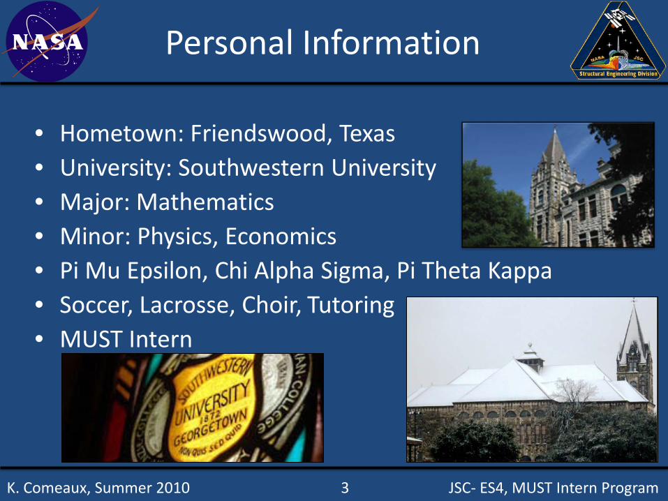
• Hometown: Friendswood, Texas• University: Southwestern University• Major: Mathematics• Minor: Physics, Economics• Pi Mu Epsilon, Chi Alpha Sigma, Pi Theta Kappa• Soccer, Lacrosse, Choir, Tutoring• MUST Intern
K. Comeaux, Summer 2010 3 JSC- ES4, MUST Intern Program
Project Objectives
K. Comeaux, Summer 2010 4 JSC- ES4, MUST Intern Program
• Simulate Flash Thermography on Graphite/Epoxy Flat Bottom hole Specimen and thin void specimens.
• Obtain Flash Thermography data on Graphite/Epoxy flat bottom hole specimens
• Compare experimental results with simulation results
• Compare Flat Bottom Hole Simulation with Thin Void Simulation to create a graph to determine size of IR Thermography detected defects
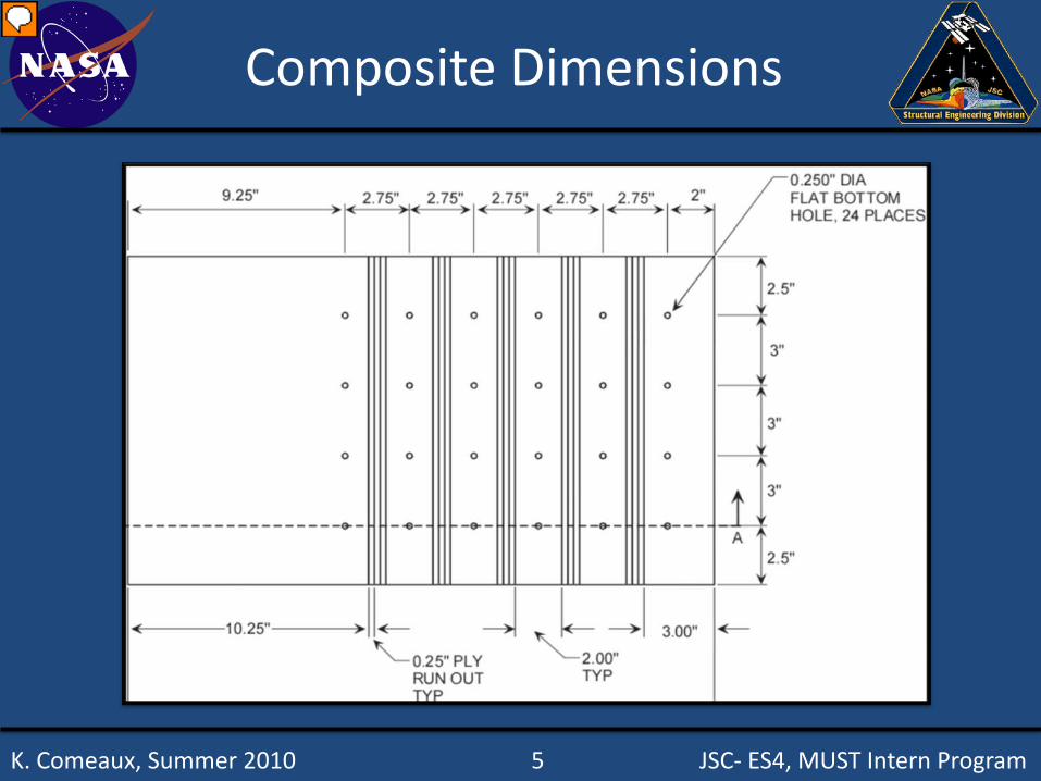
Composite Dimensions
K. Comeaux, Summer 2010 5 JSC- ES4, MUST Intern Program
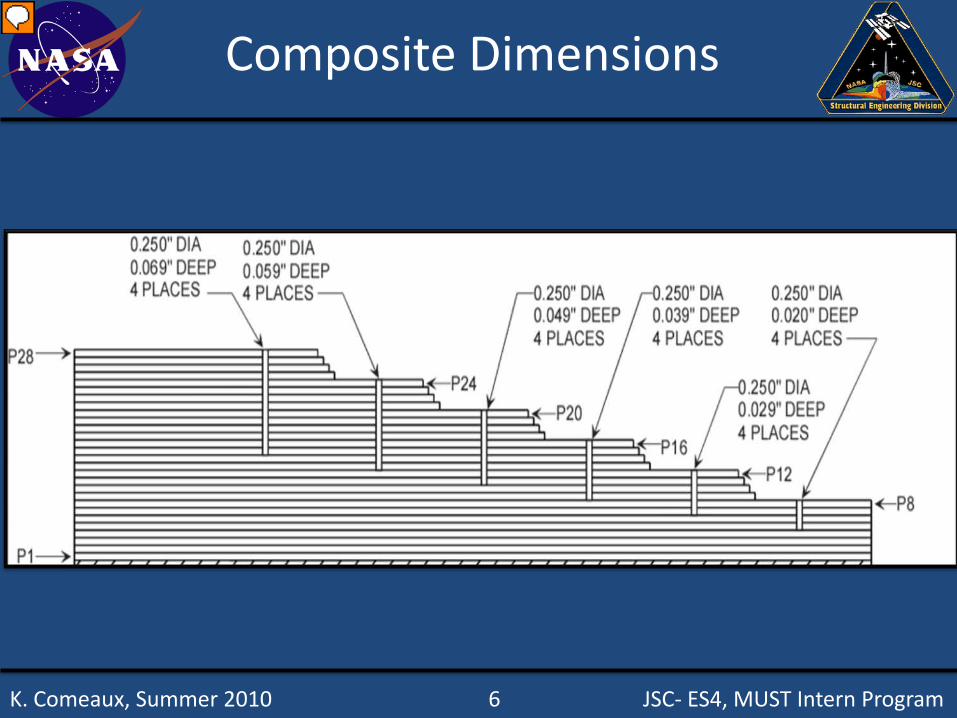
Composite Dimensions
K. Comeaux, Summer 2010 6 JSC- ES4, MUST Intern Program
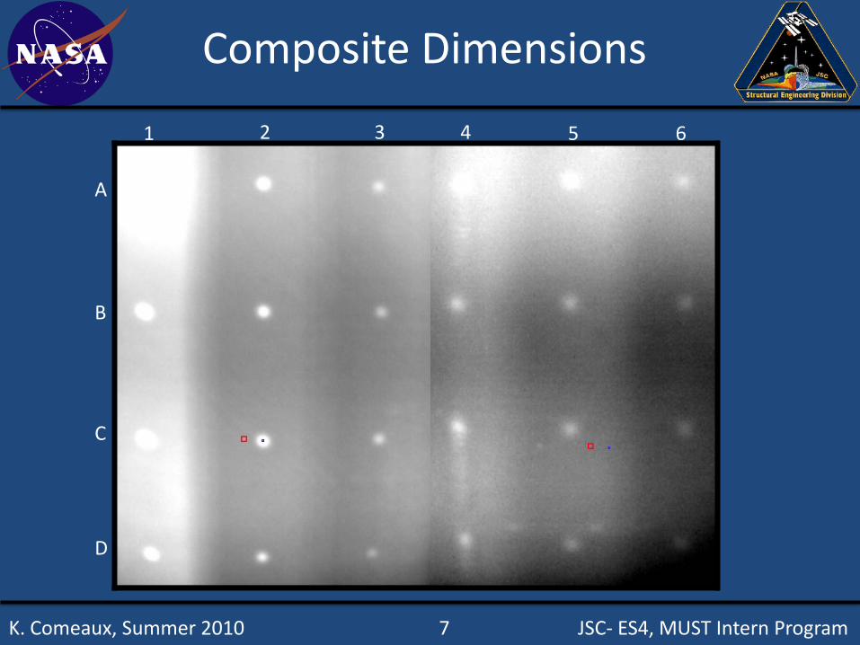
Composite Dimensions
K. Comeaux, Summer 2010 7 JSC- ES4, MUST Intern Program
1 2 3 4 5 6
A
B
C
D
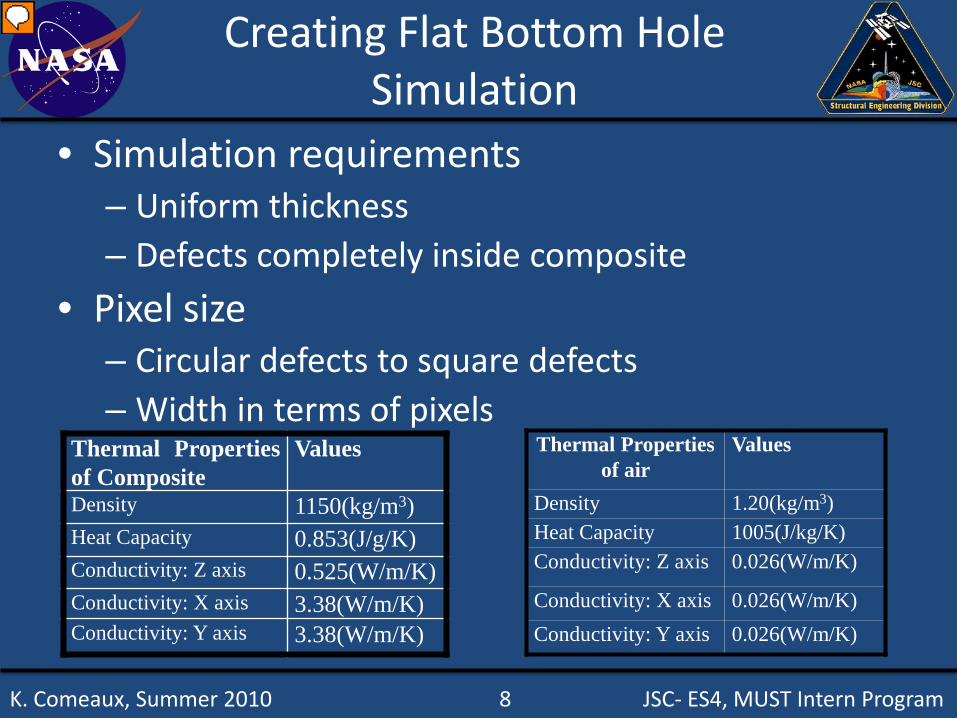
Creating Flat Bottom Hole Simulation
• Simulation requirements– Uniform thickness– Defects completely inside composite
• Pixel size– Circular defects to square defects– Width in terms of pixels
K. Comeaux, Summer 2010 8 JSC- ES4, MUST Intern Program
Thermal Propertiesof Composite
Values
Density 1150(kg/m3)Heat Capacity 0.853(J/g/K)Conductivity: Z axis 0.525(W/m/K)Conductivity: X axis 3.38(W/m/K)Conductivity: Y axis 3.38(W/m/K)
Thermal Properties of air
Values
Density 1.20(kg/m3)Heat Capacity 1005(J/kg/K)Conductivity: Z axis 0.026(W/m/K)
Conductivity: X axis 0.026(W/m/K)Conductivity: Y axis 0.026(W/m/K)
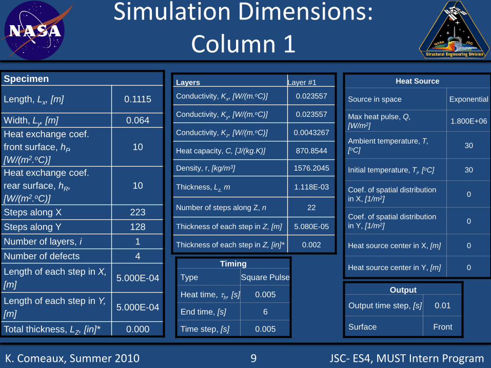
Simulation Dimensions: Column 1
K. Comeaux, Summer 2010 9 JSC- ES4, MUST Intern Program
Layers Layer #1
Conductivity, Kx, [W/(m.oC)] 0.023557
Conductivity, Ky, [W/(m.oC)] 0.023557
Conductivity, Kz, [W/(m.oC)] 0.0043267
Heat capacity, C, [J/(kg.K)] 870.8544
Density, r, [kg/m3] 1576.2045
Thickness, Lz, m 1.118E-03
Number of steps along Z, n 22
Thickness of each step in Z, [m] 5.080E-05
Thickness of each step in Z, [in]* 0.002
Specimen
Length, Lx, [m] 0.1115
Width, Ly, [m] 0.064Heat exchange coef. front surface, hF, [W/(m2.oC)]
10
Heat exchange coef. rear surface, hR, [W/(m2.oC)]
10
Steps along X 223Steps along Y 128Number of layers, i 1Number of defects 4Length of each step in X, [m]
5.000E-04
Length of each step in Y, [m]
5.000E-04
Total thickness, LZ, [in]* 0.000
TimingType Square Pulse
Heat time, τh, [s] 0.005
End time, [s] 6
Time step, [s] 0.005
Heat Source
Source in space Exponential
Max heat pulse, Q, [W/m2] 1.800E+06
Ambient temperature, T, [oC] 30
Initial temperature, Ti, [oC] 30
Coef. of spatial distribution in X, [1/m2] 0
Coef. of spatial distribution in Y, [1/m2] 0
Heat source center in X, [m] 0
Heat source center in Y, [m] 0
Output
Output time step, [s] 0.01
Surface Front
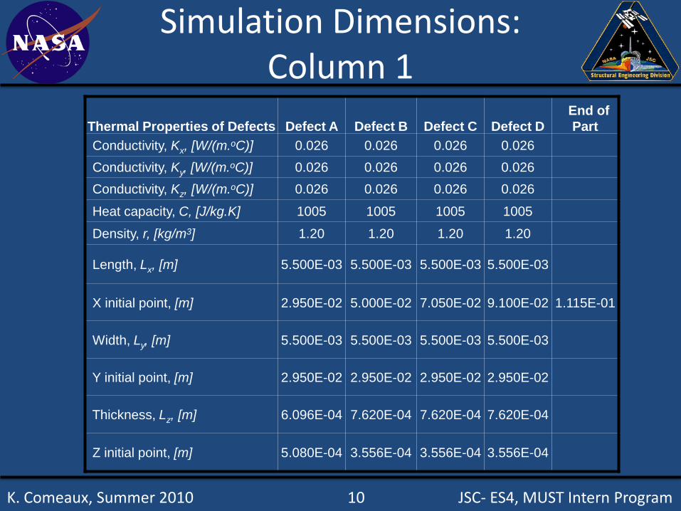
Simulation Dimensions: Column 1
K. Comeaux, Summer 2010 10 JSC- ES4, MUST Intern Program
Thermal Properties of Defects Defect A Defect B Defect C Defect DEnd of Part
Conductivity, Kx, [W/(m.oC)] 0.026 0.026 0.026 0.026Conductivity, Ky, [W/(m.oC)] 0.026 0.026 0.026 0.026Conductivity, Kz, [W/(m.oC)] 0.026 0.026 0.026 0.026
Heat capacity, C, [J/kg.K] 1005 1005 1005 1005
Density, r, [kg/m3] 1.20 1.20 1.20 1.20
Length, Lx, [m] 5.500E-03 5.500E-03 5.500E-03 5.500E-03
X initial point, [m] 2.950E-02 5.000E-02 7.050E-02 9.100E-02 1.115E-01
Width, Ly, [m] 5.500E-03 5.500E-03 5.500E-03 5.500E-03
Y initial point, [m] 2.950E-02 2.950E-02 2.950E-02 2.950E-02
Thickness, Lz, [m] 6.096E-04 7.620E-04 7.620E-04 7.620E-04
Z initial point, [m] 5.080E-04 3.556E-04 3.556E-04 3.556E-04
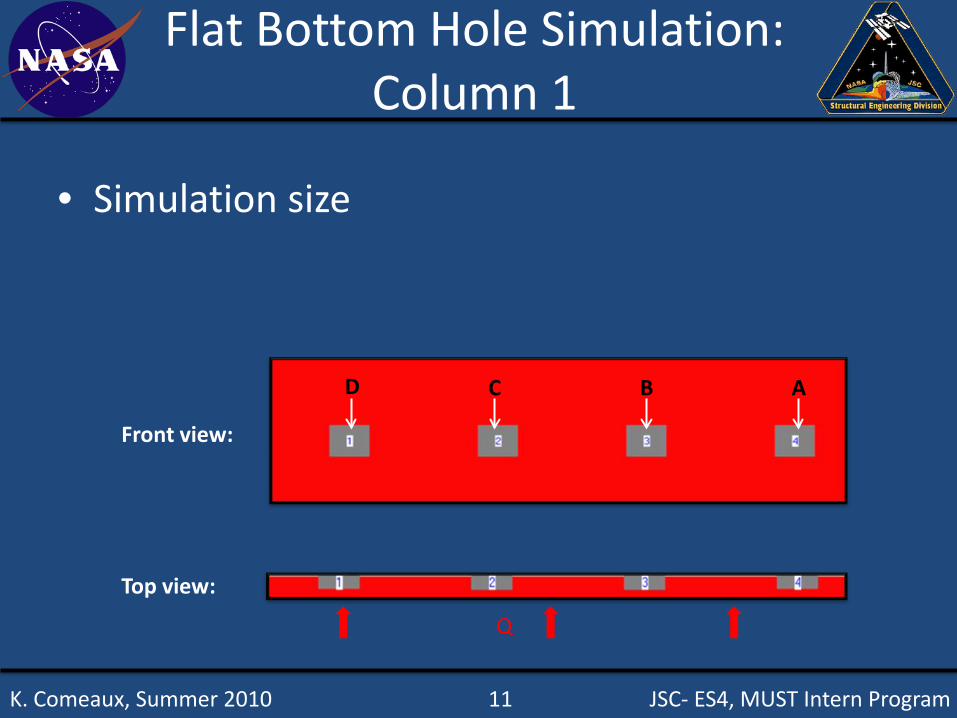
• Simulation size
Front view:
Top view:
Flat Bottom Hole Simulation: Column 1
K. Comeaux, Summer 2010 11 JSC- ES4, MUST Intern Program
D C B A
Q
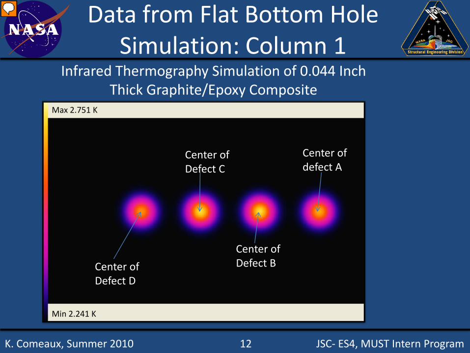
Data from Flat Bottom Hole Simulation: Column 1
Infrared Thermography Simulation of 0.044 Inch Thick Graphite/Epoxy Composite
Center of Defect D
Center of Defect C
Center of Defect B
Center of defect A
Min 2.241 K
Max 2.751 K
K. Comeaux, Summer 2010 12 JSC- ES4, MUST Intern Program
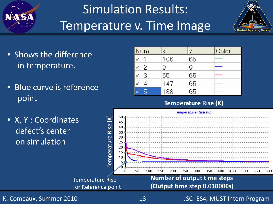
Simulation Results: Temperature v. Time Image
• Shows the difference in temperature.
• Blue curve is reference point
• X, Y : Coordinates defect’s center on simulation
Tem
pera
ture
Ris
e (K
)
Number of output time steps(Output time step 0.010000s)
Temperature Rise (K)
Temperature Rise for Reference point
K. Comeaux, Summer 2010 13 JSC- ES4, MUST Intern Program
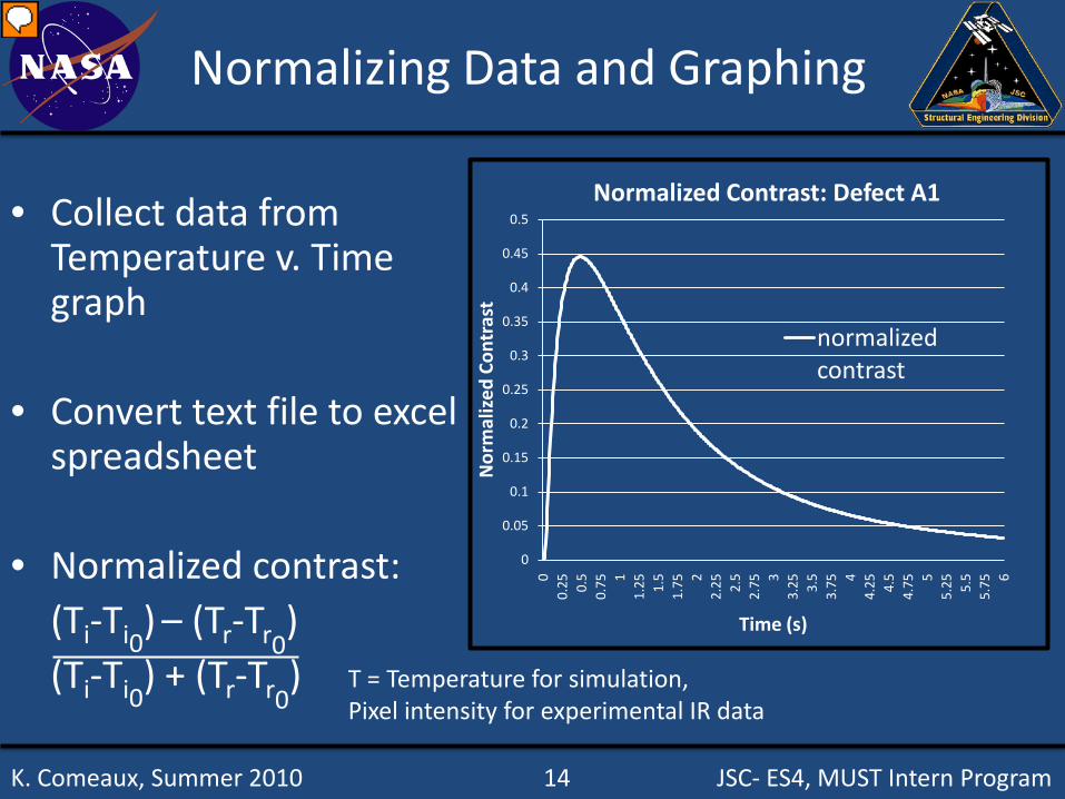
Normalizing Data and Graphing
• Collect data from Temperature v. Time graph
• Convert text file to excel spreadsheet
• Normalized contrast:(Ti-Ti0
) – (Tr-Tr0)
(Ti-Ti0) + (Tr-Tr0
)
0
0.05
0.1
0.15
0.2
0.25
0.3
0.35
0.4
0.45
0.5
00.
25 0.5
0.75 1
1.25 1.
51.
75 22.
25 2.5
2.75 3
3.25 3.
53.
75 44.
25 4.5
4.75 5
5.25 5.
55.
75 6
Nor
mal
ized
Con
tras
t
Time (s)
Normalized Contrast: Defect A1
normalized contrast
K. Comeaux, Summer 2010 14 JSC- ES4, MUST Intern Program
T = Temperature for simulation,Pixel intensity for experimental IR data
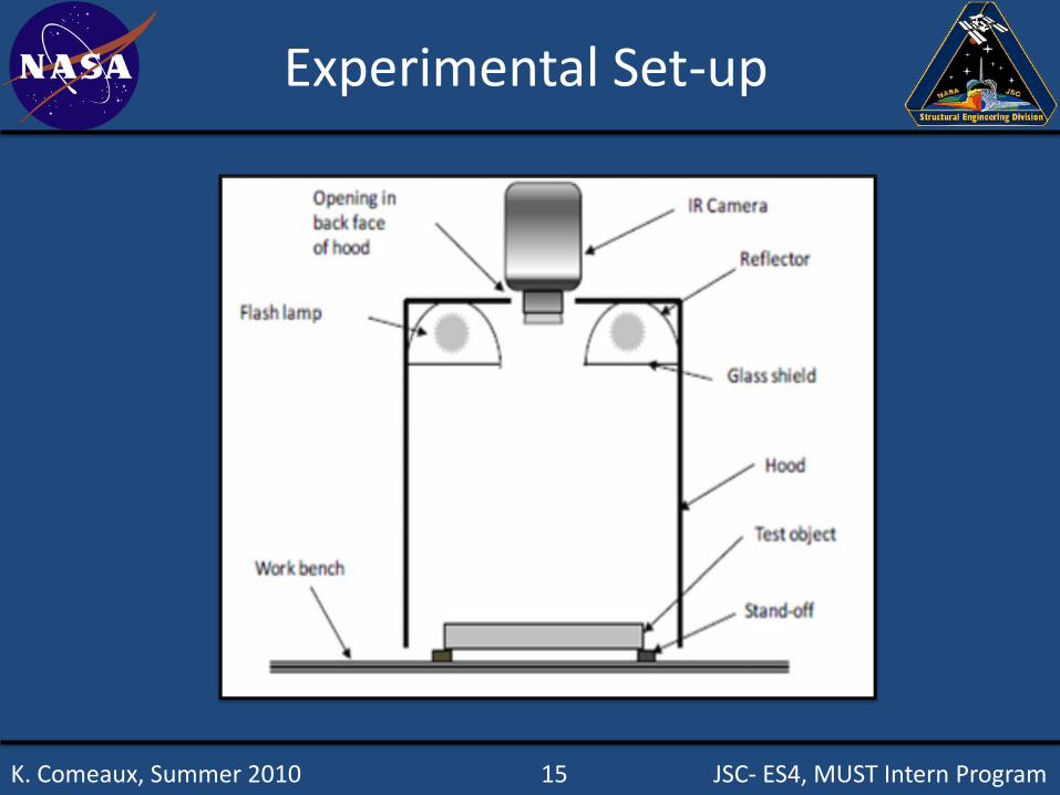
Experimental Set-up
K. Comeaux, Summer 2010 15 JSC- ES4, MUST Intern Program
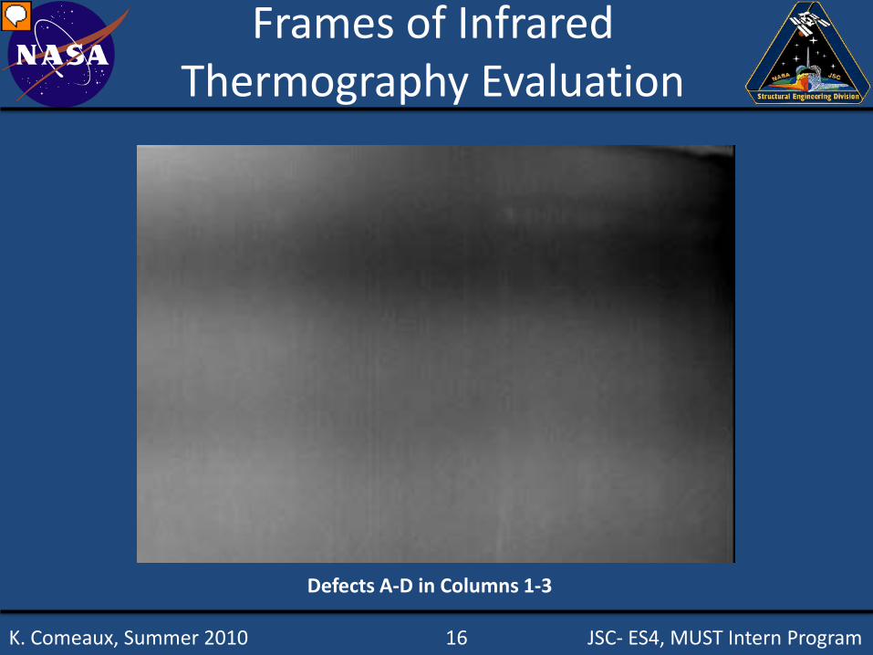
Frames of Infrared Thermography Evaluation
K. Comeaux, Summer 2010 16 JSC- ES4, MUST Intern Program
Defects A-D in Columns 1-3
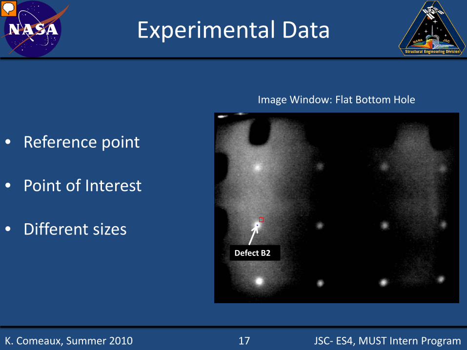
Experimental Data
K. Comeaux, Summer 2010 17 JSC- ES4, MUST Intern Program
Defect B2
• Reference point
• Point of Interest
• Different sizes
Image Window: Flat Bottom Hole
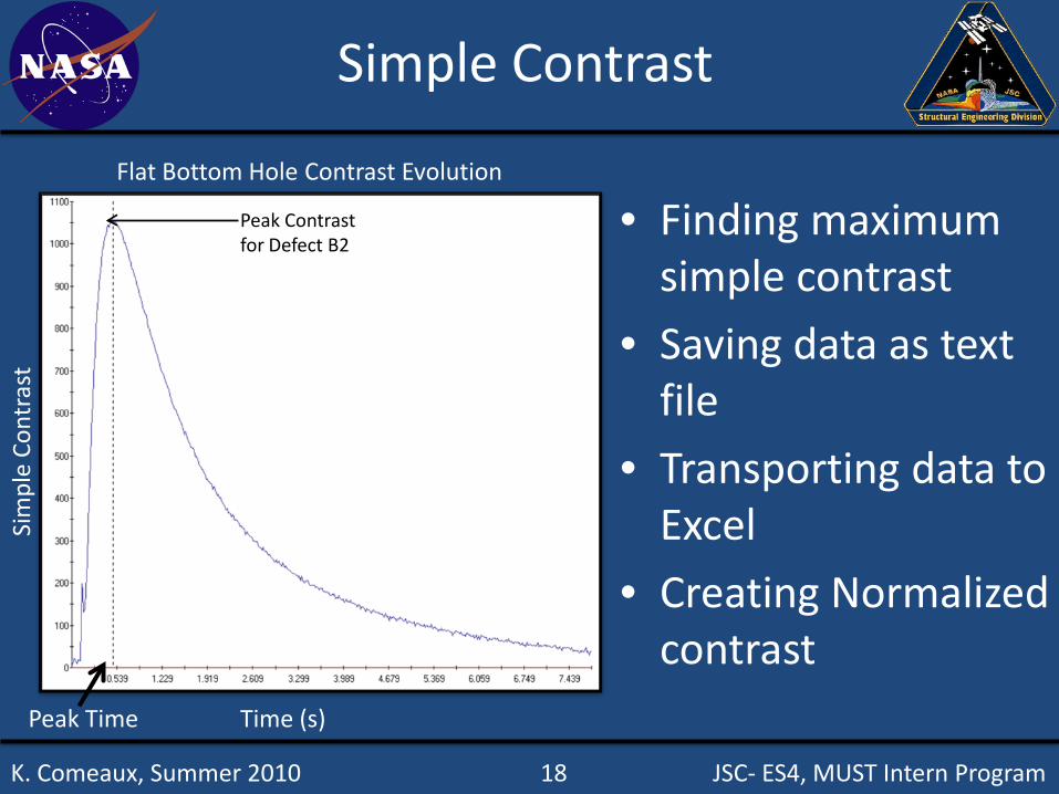
• Finding maximum simple contrast
• Saving data as text file
• Transporting data to Excel
• Creating Normalized contrast
Flat Bottom Hole Contrast Evolution
Time (s)
Sim
ple
Cont
rast
Peak Contrast for Defect B2
Peak Time
Simple Contrast
K. Comeaux, Summer 2010 18 JSC- ES4, MUST Intern Program
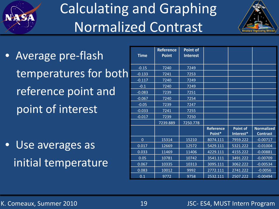
Calculating and Graphing Normalized Contrast
• Average pre-flash
temperatures for both
reference point and
point of interest
• Use averages as
initial temperature
K. Comeaux, Summer 2010 19 JSC- ES4, MUST Intern Program
TimeReference
PointPoint of Interest
-0.15 7240 7249-0.133 7241 7253-0.117 7240 7249
-0.1 7240 7249-0.083 7239 7251-0.067 7240 7254-0.05 7239 7247
-0.033 7241 7255-0.017 7239 7250
7239.889 7250.778Reference
Point*Point of
Interest*Normalized
Contrast0 15314 15210 8074.111 7959.222 -0.00717
0.017 12669 12572 5429.111 5321.222 -0.010040.033 11469 11406 4229.111 4155.222 -0.008810.05 10781 10742 3541.111 3491.222 -0.00709
0.067 10335 10313 3095.111 3062.222 -0.005340.083 10012 9992 2772.111 2741.222 -0.0056
0.1 9772 9758 2532.111 2507.222 -0.00494
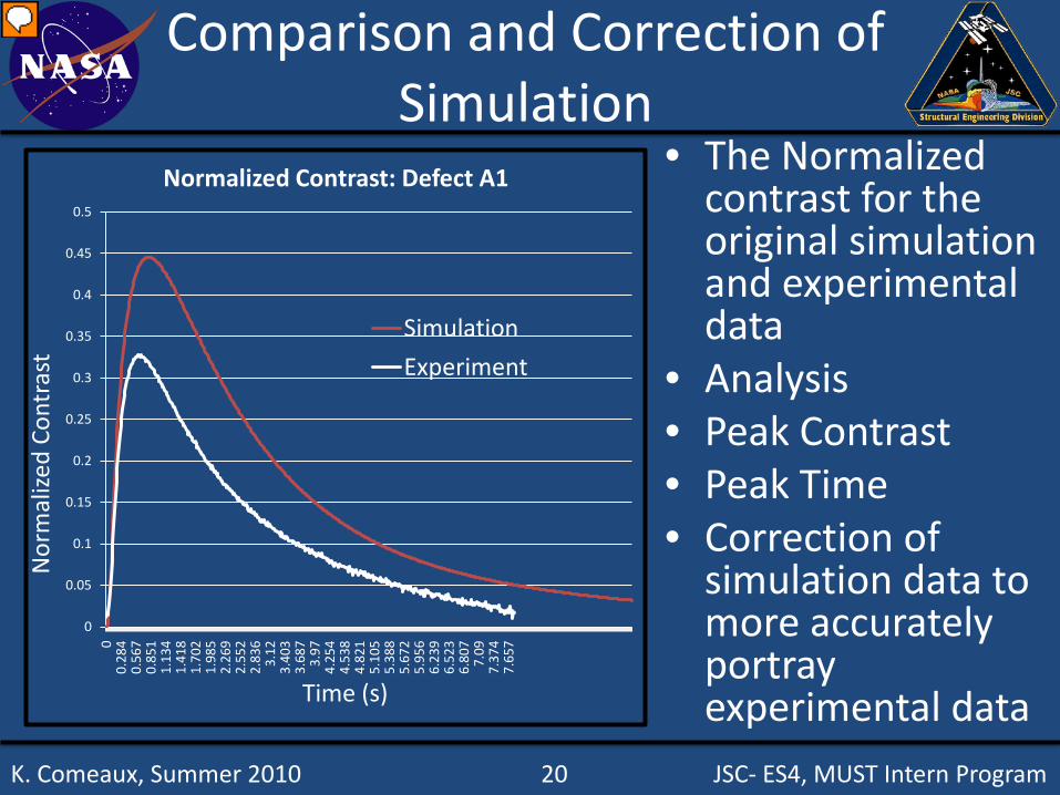
Comparison and Correction of Simulation
• The Normalized contrast for the original simulation and experimental data
• Analysis• Peak Contrast• Peak Time• Correction of
simulation data to more accurately portray experimental data
K. Comeaux, Summer 2010 20 JSC- ES4, MUST Intern Program
0
0.05
0.1
0.15
0.2
0.25
0.3
0.35
0.4
0.45
0.5
00.
284
0.56
70.
851
1.13
41.
418
1.70
21.
985
2.26
92.
552
2.83
63.
123.
403
3.68
73.
974.
254
4.53
84.
821
5.10
55.
388
5.67
25.
956
6.23
96.
523
6.80
77.
097.
374
7.65
7
Normalized Contrast: Defect A1
Simulation
Experiment
Nor
mal
ized
Con
tras
t
Time (s)
Correction of Simulation
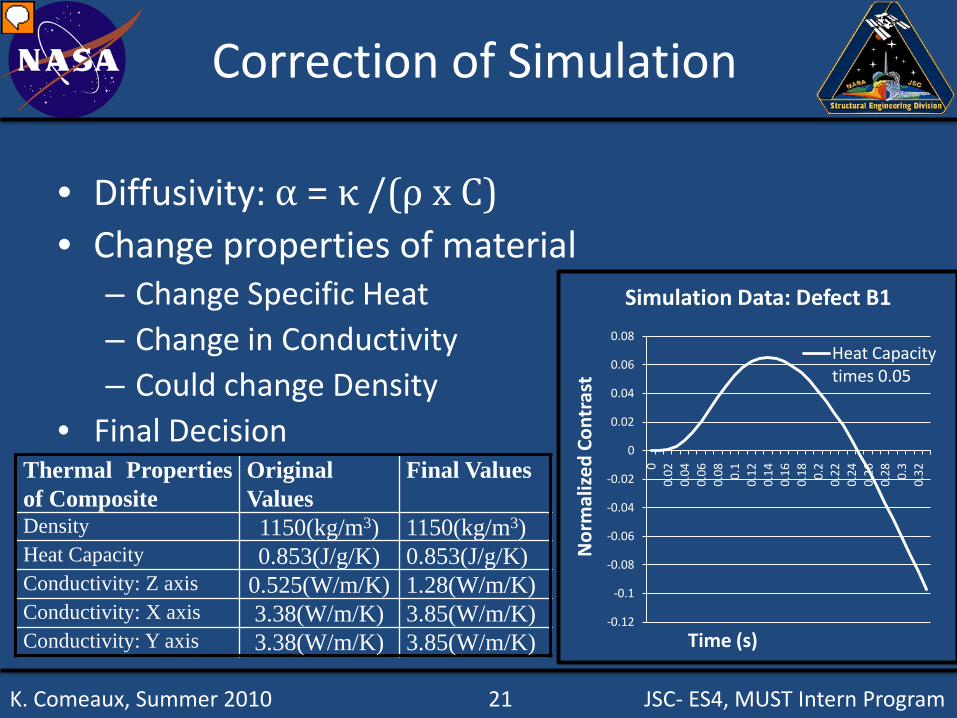
• Diffusivity: α = κ /(ρ x С)• Change properties of material
– Change Specific Heat– Change in Conductivity– Could change Density
• Final DecisionThermal Propertiesof Composite
OriginalValues
Final Values
Density 1150(kg/m3) 1150(kg/m3)Heat Capacity 0.853(J/g/K) 0.853(J/g/K)Conductivity: Z axis 0.525(W/m/K) 1.28(W/m/K)Conductivity: X axis 3.38(W/m/K) 3.85(W/m/K)Conductivity: Y axis 3.38(W/m/K) 3.85(W/m/K)
-0.12
-0.1
-0.08
-0.06
-0.04
-0.02
0
0.02
0.04
0.06
0.08
00.
020.
040.
060.
08 0.1
0.12
0.14
0.16
0.18 0.
20.
220.
240.
260.
28 0.3
0.32
Simulation Data: Defect B1
Heat Capacity times 0.05
Time (s)
Nor
mal
ized
Con
tras
t
K. Comeaux, Summer 2010 21 JSC- ES4, MUST Intern Program
0
0.05
0.1
0.15
0.2
0.25
0.3
0.35
0.4
0.45
0.5
00.
30.
601
0.90
11.
201
1.50
11.
802
2.10
22.
402
2.70
33.
003
3.30
33.
603
3.90
44.
204
4.50
44.
805
5.10
55.
405
5.70
56.
006
6.30
66.
606
6.90
77.
207
7.50
7
Nor
mal
ized
Con
tras
t
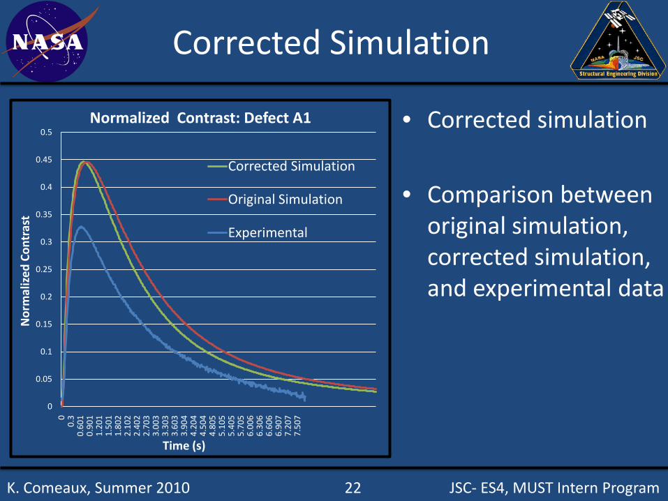
Normalized Contrast: Defect A1
Corrected Simulation
Original Simulation
Experimental
Corrected Simulation
• Corrected simulation
• Comparison between original simulation, corrected simulation, and experimental data
K. Comeaux, Summer 2010 22 JSC- ES4, MUST Intern Program
Time (s)
• Simulation contrast is based on temperature versus time. Experimental contrast is based on pixel intensity versus time.
• Experimental Flash vs. Simulation Flash– Experimental flash envelope has a sharp rise and slow decay– Simulation flash is a square pulse
• Experimental factors– Experimental data is more sensitive to pixel size. Get smaller pixel
intensity for a larger pixel– Uneven flash causes some lateral heat flow– Part has a surface texture causing lateral heat flow
• Emissivity– The specimen emissivity was measured to be 0.9 and provides
lower (< 5%) experimental contrast • Simulation inaccuracies (model approximations, boundary condition
approximations, no lateral heat flow)
Sources of Differences
K. Comeaux, Summer 2010 23 JSC- ES4, MUST Intern Program
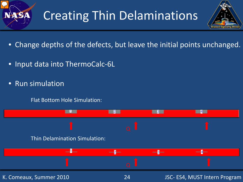
Creating Thin Delaminations
Flat Bottom Hole Simulation:
Thin Delamination Simulation:
K. Comeaux, Summer 2010 24 JSC- ES4, MUST Intern Program
Q
Q
• Change depths of the defects, but leave the initial points unchanged.
• Input data into ThermoCalc-6L
• Run simulation
• Same as for the flat bottom hole simulation– Collect data from Temperature v. Time graph for
each defect
– Convert the text file to excel spreadsheet compatible
– Generate normalized contrast graph
Collecting Data
K. Comeaux, Summer 2010 25 JSC- ES4, MUST Intern Program
• Comparing flat bottom hole simulation to thin delamination simulation
• Compare and graph the peak contrast ratio and peak time ratio– Thin delamination/Flat bottom hole
Comparison of Simulations
K. Comeaux, Summer 2010 26 JSC- ES4, MUST Intern Program
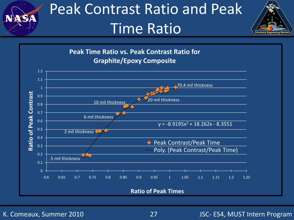
Peak Contrast Ratio and Peak Time Ratio
K. Comeaux, Summer 2010 27 JSC- ES4, MUST Intern Program
y = -8.9195x2 + 18.262x - 8.3551
0
0.1
0.2
0.3
0.4
0.5
0.6
0.7
0.8
0.9
1
1.1
1.2
0.6 0.65 0.7 0.75 0.8 0.85 0.9 0.95 1 1.05 1.1 1.15 1.2 1.25
Rati
o of
Pea
k Co
ntra
st
Ratio of Peak Times
Peak Time Ratio vs. Peak Contrast Ratio for Graphite/Epoxy Composite
Peak Contrast/Peak TimePoly. (Peak Contrast/Peak Time)
.5 mil thickness
70.4 mil thickness
2 mil thickness
6 mil thickness
10 mil thickness 20 mil thickness
Future Work
• Make controlled impacts to make thin delaminations
• Evaluate delaminations with Infrared Thermography
• Evaluate delaminations with Ultrasonic Techniques
• Section the specimen at delaminations• Determine actual size of delaminations• Compare actual results with simulated results• Determine accuracy of the simulation
K. Comeaux, Summer 2010 28 JSC- ES4, MUST Intern Program
• Learned Thermodynamics– Theory and application
• IR temperature measurement
• Infrared Thermography NDE – Simulation– IR Experimental data acquisition and analysis
• Eddy Current• Ultrasonic Testing• Time management• Work hours• Technical paper
Skills Acquired
K. Comeaux, Summer 2010 29 JSC- ES4, MUST Intern Program

Experiences at JSC
Building 14:
Boom Tower
NBLMission Control
Apollo
Ellington Field
GuppyONWG Meetings
Building 1
Movie Night
MusicalsMLS All-Stars vs
Volunteering
Food Bank
K. Comeaux, Summer 2010 30 JSC- ES4, MUST Intern Program
Tutoring
CLPCDay of Service
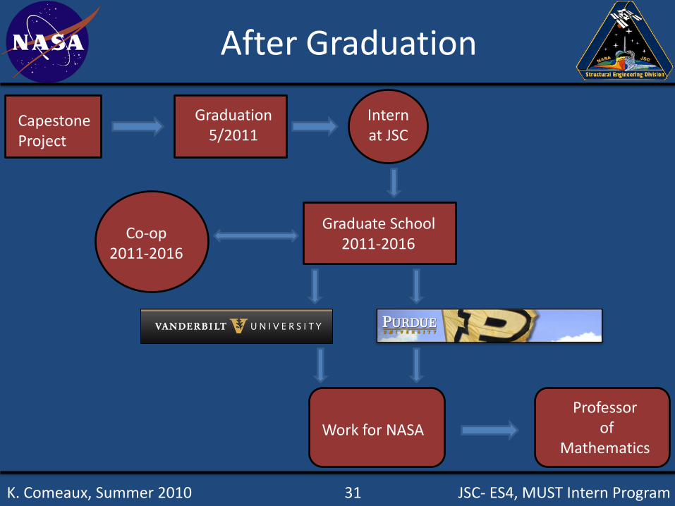
After Graduation
Professorof
Mathematics
Graduation5/2011
Intern at JSC
Graduate School 2011-2016
Co-op2011-2016
Work for NASA
K. Comeaux, Summer 2010 31 JSC- ES4, MUST Intern Program
CapestoneProject
Acknowledgements
• Parents and Family
• Mentors: Ajay Koshti & David Stanley
• Ovidio Olveras, Eddie Pompa, Norman Ruffino, Rodrigo Devivar, John Figert, Budd Castner, Mike Kocurek, Denise Plantier, Erica Worthy, Joseph Prather
• MUST Point of Contact: Cornelius Johnson
K. Comeaux, Summer 2010 32 JSC- ES4, MUST Intern Program
Exit Presentation: Infrared Thermography on Graphite/Epoxy
Thank You
K. Comeaux, Summer 2010 33 JSC- ES4, MUST Intern Program