DOCUMENT FLASH THERMOGRAPHY

by

Cory A. Larsen

A thesis submitted in partial fulfillmentof the requirements for the degree

of

MASTER OF SCIENCE

in

Electrical Engineering

Approved:

Dr. Doran J. Baker Dr. Gene A. WareMajor Professor Committee Member

Dr. Todd Moon Dr. Mark R. McLellanCommittee Member Vice President for Research and

Dean of the School of Graduate Studies

UTAH STATE UNIVERSITYLogan, Utah

2011

ii

Copyright c© Cory A. Larsen 2011

All Rights Reserved

iii

Abstract

Document Flash Thermography

by

Cory A. Larsen, Master of Science

Utah State University, 2011

Major Professor: Dr. Doran J. BakerDepartment: Electrical and Computer Engineering

This thesis presents the application of flash thermography techniques to the analysis of

documents. The motivation for this research is to develop the ability to non-destructively

reveal covered writings in archaeological artifacts such as the Codex Selden or Egyptian car-

tonnage. Current common signal processing techniques are evaluated for their effectiveness

in enhancing subsurface writings found within a set of test documents. These processing

techniques include: false colorization, contrast stretching, histogram equalization, median

filtering, Gaussian low-pass filtering, layered signal reconstruction and thermal signal recon-

struction (TSR), several contrast image definitions, differential absolute contrast (DAC),

correlated contrast, derivative images, principal component thermography (PCT), dynamic

thermal tomography (DTT), pulse phase thermography (PPT), fitting-correlation analy-

sis (FCA), Hough transform thermography (PTHTa), and transmission line matrix fitting

algorithm (TLMFa). New processing techniques are developed and evaluated against the

existing techniques. The ability of flash thermography coupled with processing techniques

to reveal subsurface writings and document strikeouts is evaluated. Flash thermography

parameters are evaluated to determine most effective value for the document.

In summary, this thesis reports the following contributions to the existing scientific

knowledge:

iv

1. A comprehensive analysis of existing pulsed thermography processing techniques.

2. New pulsed thermography processing techniques that improve upon the results of the

existing techniques were developed.

3. A proof-of-concept for detecting subsurface ink writings in documents.

4. Verifies the capability of pulsed thermography techniques to detect document strike-

outs.

5. Demonstrates the ability to enhance surface writings based on differences in thermal

characteristics when optical characteristics do not differ significantly.

6. Demonstrates that pulsed thermography significantly improves upon multi-spectral

imaging for subsurface and surface writing enhancement.

7. Provides an evaluation of flash thermography parameters for the most effective doc-

ument imaging.

(146 pages)

v

Acknowledgments

Special thanks to Pedro Sevilla and James Peterson of the Space Dynamics Labora-

tory for the use of their equipment and helping with the acquisition of the thermal images.

Thank you to Dr. Gene A. Ware for his mentorship and guidance throughout the project.

Thanks to Dr. Doran J. Baker of the Rocky Mountain NASA Spacegrant Consortium for

funding the research and providing assistance as needed. Finally, thanks goes to Dr. Todd

Moon and Dr. Jake Gunther of Utah State University for sharing their advice and expertise.

Cory A. Larsen

vi

Contents

Page

Abstract . . . . . . . . . . . . . . . . . . . . . . . . . . . . . . . . . . . . . . . . . . . . . . . . . . . . . . . iii

Acknowledgments . . . . . . . . . . . . . . . . . . . . . . . . . . . . . . . . . . . . . . . . . . . . . . . v

List of Tables . . . . . . . . . . . . . . . . . . . . . . . . . . . . . . . . . . . . . . . . . . . . . . . . . . . ix

List of Figures . . . . . . . . . . . . . . . . . . . . . . . . . . . . . . . . . . . . . . . . . . . . . . . . . . x

Acronyms . . . . . . . . . . . . . . . . . . . . . . . . . . . . . . . . . . . . . . . . . . . . . . . . . . . . . . xiii

1 Introduction . . . . . . . . . . . . . . . . . . . . . . . . . . . . . . . . . . . . . . . . . . . . . . . . . 11.1 General Background . . . . . . . . . . . . . . . . . . . . . . . . . . . . . . . 11.2 Problem Statement . . . . . . . . . . . . . . . . . . . . . . . . . . . . . . . . 11.3 Research Objectives . . . . . . . . . . . . . . . . . . . . . . . . . . . . . . . 21.4 Literature Review . . . . . . . . . . . . . . . . . . . . . . . . . . . . . . . . 2

1.4.1 Document Imaging and MSI . . . . . . . . . . . . . . . . . . . . . . 31.4.2 Flash Thermography Processing Algorithms . . . . . . . . . . . . . . 4

2 General Pulsed Thermography Considerations . . . . . . . . . . . . . . . . . . . . . 62.1 Terminology . . . . . . . . . . . . . . . . . . . . . . . . . . . . . . . . . . . . 62.2 Instrumentation Requirements . . . . . . . . . . . . . . . . . . . . . . . . . 62.3 Flash Thermography Design Variables . . . . . . . . . . . . . . . . . . . . . 7

2.3.1 Thermal Imager Characteristics . . . . . . . . . . . . . . . . . . . . . 72.3.2 Thermal Properties of the Target . . . . . . . . . . . . . . . . . . . . 92.3.3 Characteristics of the Transmitting Medium . . . . . . . . . . . . . . 102.3.4 Excitation Pulse Characteristics . . . . . . . . . . . . . . . . . . . . 10

3 Experiment Setup . . . . . . . . . . . . . . . . . . . . . . . . . . . . . . . . . . . . . . . . . . . . . 133.1 Instrumentation Used . . . . . . . . . . . . . . . . . . . . . . . . . . . . . . 133.2 Target Documents . . . . . . . . . . . . . . . . . . . . . . . . . . . . . . . . 13

3.2.1 Subsurface Imaging . . . . . . . . . . . . . . . . . . . . . . . . . . . 143.2.2 Strikeouts . . . . . . . . . . . . . . . . . . . . . . . . . . . . . . . . . 143.2.3 Surface Ink Enhancement . . . . . . . . . . . . . . . . . . . . . . . . 153.2.4 Egyptian Cartonnage . . . . . . . . . . . . . . . . . . . . . . . . . . 15

4 Processing Techniques . . . . . . . . . . . . . . . . . . . . . . . . . . . . . . . . . . . . . . . . . 174.1 Background Theory . . . . . . . . . . . . . . . . . . . . . . . . . . . . . . . 174.2 Existing Techniques . . . . . . . . . . . . . . . . . . . . . . . . . . . . . . . 18

4.2.1 Pseudo-Color Images . . . . . . . . . . . . . . . . . . . . . . . . . . . 184.2.2 Contrast Stretching . . . . . . . . . . . . . . . . . . . . . . . . . . . 194.2.3 Histogram Equalization . . . . . . . . . . . . . . . . . . . . . . . . . 20

vii

4.2.4 Image Filters . . . . . . . . . . . . . . . . . . . . . . . . . . . . . . . 214.2.5 Synthetic Signal Reconstruction Techniques . . . . . . . . . . . . . . 214.2.6 Contrast Definitions . . . . . . . . . . . . . . . . . . . . . . . . . . . 234.2.7 Differential Absolute Contrast (DAC) . . . . . . . . . . . . . . . . . 244.2.8 Derivative Images . . . . . . . . . . . . . . . . . . . . . . . . . . . . 254.2.9 Principal Component Thermography (PCT) . . . . . . . . . . . . . . 264.2.10 Dynamic Thermal Tomography (DTT) . . . . . . . . . . . . . . . . . 274.2.11 Pulse Phase Thermography (PPT) . . . . . . . . . . . . . . . . . . . 284.2.12 Correlation Images . . . . . . . . . . . . . . . . . . . . . . . . . . . . 304.2.13 Transmission Line Matrix Fitting Algorithm (TLMFa) . . . . . . . . 314.2.14 Hough Transform Thermography (PTHTa) . . . . . . . . . . . . . . 33

4.3 Developed Techniques . . . . . . . . . . . . . . . . . . . . . . . . . . . . . . 344.3.1 Time-Difference Contrast . . . . . . . . . . . . . . . . . . . . . . . . 344.3.2 Total Harmonic Distortion (THD) . . . . . . . . . . . . . . . . . . . 354.3.3 Markov Error Contrast (MEC) . . . . . . . . . . . . . . . . . . . . . 364.3.4 Time Constant Analysis (TCA) . . . . . . . . . . . . . . . . . . . . . 374.3.5 Signal Detection and Matched Filtering (MF) . . . . . . . . . . . . . 374.3.6 Convex Optimization Signal Detection Technique . . . . . . . . . . . 41

5 Analysis of Results . . . . . . . . . . . . . . . . . . . . . . . . . . . . . . . . . . . . . . . . . . . . 435.1 Processing Techniques Results . . . . . . . . . . . . . . . . . . . . . . . . . . 43

5.1.1 Subsurface Inks . . . . . . . . . . . . . . . . . . . . . . . . . . . . . . 435.1.2 Document Strikeouts . . . . . . . . . . . . . . . . . . . . . . . . . . . 55

5.2 Comparison of Algorithm Wall Times . . . . . . . . . . . . . . . . . . . . . 625.3 Comparison with Multi-Spectral Imaging (MSI) . . . . . . . . . . . . . . . . 62

5.3.1 Subsurface Inks . . . . . . . . . . . . . . . . . . . . . . . . . . . . . . 625.3.2 Document Strikeouts . . . . . . . . . . . . . . . . . . . . . . . . . . . 675.3.3 Surface Writing Enhancement . . . . . . . . . . . . . . . . . . . . . . 67

5.4 Feasibility of Application to Archaeological Artifacts . . . . . . . . . . . . . 695.4.1 Egyptian Cartonnage . . . . . . . . . . . . . . . . . . . . . . . . . . 695.4.2 Codex Selden . . . . . . . . . . . . . . . . . . . . . . . . . . . . . . . 71

6 Conclusions and Recommendations . . . . . . . . . . . . . . . . . . . . . . . . . . . . . . 776.1 Thermography Data Acquisition Parameters . . . . . . . . . . . . . . . . . . 776.2 Pre-Processing . . . . . . . . . . . . . . . . . . . . . . . . . . . . . . . . . . 786.3 Processing . . . . . . . . . . . . . . . . . . . . . . . . . . . . . . . . . . . . . 786.4 Post-Processing . . . . . . . . . . . . . . . . . . . . . . . . . . . . . . . . . . 786.5 Materials . . . . . . . . . . . . . . . . . . . . . . . . . . . . . . . . . . . . . 796.6 Significant Contributions . . . . . . . . . . . . . . . . . . . . . . . . . . . . . 796.7 Recommendations for Future Research . . . . . . . . . . . . . . . . . . . . . 81

References . . . . . . . . . . . . . . . . . . . . . . . . . . . . . . . . . . . . . . . . . . . . . . . . . . . . . . 83

Appendices . . . . . . . . . . . . . . . . . . . . . . . . . . . . . . . . . . . . . . . . . . . . . . . . . . . . . 92Appendix A Pulsed Thermography Toolbox . . . . . . . . . . . . . . . . . . . 93

A.1 Pulsed Thermography Toolbox (PTT) Introduction . . . . . . . . . 93A.2 Load Images . . . . . . . . . . . . . . . . . . . . . . . . . . . . . . . 93

viii

A.3 Manually Manipulate Data Panel . . . . . . . . . . . . . . . . . . . . 95A.4 Pre-Processing Panel . . . . . . . . . . . . . . . . . . . . . . . . . . . 97A.5 Processing Panel . . . . . . . . . . . . . . . . . . . . . . . . . . . . . 98A.6 Post-Processing Panel . . . . . . . . . . . . . . . . . . . . . . . . . . 98A.7 Other GUI Sub-Components . . . . . . . . . . . . . . . . . . . . . . 98A.8 Explore Data Sub-GUI . . . . . . . . . . . . . . . . . . . . . . . . . . 99

Appendix B Code Listings . . . . . . . . . . . . . . . . . . . . . . . . . . . . . 101B.1 Contrast Definitions & Differential Absolute Contrast (DAC) . . . . 101B.2 Thermal Signal Reconstruction (TSR) and Derivative Images . . . . 106B.3 Principal Component Thermography (PCT) . . . . . . . . . . . . . . 111B.4 Dynamic Thermal Tomography (DTT) . . . . . . . . . . . . . . . . . 113B.5 Pulse Phase Thermography (PPT) . . . . . . . . . . . . . . . . . . . 118B.6 Time-Difference Contrast (TDC) . . . . . . . . . . . . . . . . . . . . 120B.7 Total Harmonic Distortion (THD) . . . . . . . . . . . . . . . . . . . 122B.8 Markov Error Contrast (MEC) . . . . . . . . . . . . . . . . . . . . . 125B.9 Time Constant Analysis (TCA) . . . . . . . . . . . . . . . . . . . . . 127B.10 Matched Filters . . . . . . . . . . . . . . . . . . . . . . . . . . . . . . 129

ix

List of Tables

Table Page

5.1 Signal reconstruction wall times. . . . . . . . . . . . . . . . . . . . . . . . . 46

5.2 Algorithm wall times. . . . . . . . . . . . . . . . . . . . . . . . . . . . . . . 63

6.1 Algorithm rating system. . . . . . . . . . . . . . . . . . . . . . . . . . . . . 79

6.2 Processing algorithms summarized. . . . . . . . . . . . . . . . . . . . . . . . 82

x

List of Figures

Figure Page

2.1 Flash thermography setup. . . . . . . . . . . . . . . . . . . . . . . . . . . . 7

2.2 Document structure. . . . . . . . . . . . . . . . . . . . . . . . . . . . . . . . 11

3.1 Pulsed thermography test system. . . . . . . . . . . . . . . . . . . . . . . . 13

3.2 Egyptian cartonnage. . . . . . . . . . . . . . . . . . . . . . . . . . . . . . . 16

5.1 Test document 1. . . . . . . . . . . . . . . . . . . . . . . . . . . . . . . . . . 44

5.2 Noise reduced images at t = 228.8 ms. . . . . . . . . . . . . . . . . . . . . . 45

5.3 Pseudo-color image at t = 228.8 ms. . . . . . . . . . . . . . . . . . . . . . . 46

5.4 Contrast stretching at t = 228.8 ms. . . . . . . . . . . . . . . . . . . . . . . 47

5.5 Differential absolute contrast (DAC) images. . . . . . . . . . . . . . . . . . 47

5.6 Contrast definitions. . . . . . . . . . . . . . . . . . . . . . . . . . . . . . . . 48

5.7 Derivative images. . . . . . . . . . . . . . . . . . . . . . . . . . . . . . . . . 49

5.8 Principal component thermography (PCT) images. . . . . . . . . . . . . . . 49

5.9 Dynamic thermal tomography (DTT) images. . . . . . . . . . . . . . . . . . 50

5.10 Pulse phase thermography (PPT) image at 1.2 Hz. . . . . . . . . . . . . . . 50

5.11 Correlation images. . . . . . . . . . . . . . . . . . . . . . . . . . . . . . . . . 51

5.12 Transmission line matrix fitting algorithm (TLMFa) image. . . . . . . . . . 51

5.13 Hough transform coefficient images. . . . . . . . . . . . . . . . . . . . . . . 52

5.14 Time-difference contrast images. . . . . . . . . . . . . . . . . . . . . . . . . 52

5.15 Total harmonic distortion (THD) images. . . . . . . . . . . . . . . . . . . . 53

5.16 Markov error contrast (MEC) images. . . . . . . . . . . . . . . . . . . . . . 54

5.17 Time constant analysis (TCA) image. . . . . . . . . . . . . . . . . . . . . . 54

xi

5.18 Matched filter images. . . . . . . . . . . . . . . . . . . . . . . . . . . . . . . 56

5.19 Strikeouts test set. . . . . . . . . . . . . . . . . . . . . . . . . . . . . . . . . 56

5.20 Contrast definition strikeout images. . . . . . . . . . . . . . . . . . . . . . . 57

5.21 DAC strikeout image with t′ = 11.5 ms and t = 57.5 ms. . . . . . . . . . . . 57

5.22 DTT classical maxigram. . . . . . . . . . . . . . . . . . . . . . . . . . . . . 58

5.23 Markov error contrast (MEC) strikeout image. . . . . . . . . . . . . . . . . 59

5.24 Principal component thermography (PCT) strikeout images. . . . . . . . . . 59

5.25 Pulse phase thermography (PPT) amplitude strikeout image. . . . . . . . . 59

5.26 Transmission line matrix fitting algorithm (TLMFa) strikeout image. . . . . 60

5.27 Time constant analysis (TCA) strikeout image. . . . . . . . . . . . . . . . . 61

5.28 Time-difference contrast strikeout images. . . . . . . . . . . . . . . . . . . . 61

5.29 Strikeout derivative images . . . . . . . . . . . . . . . . . . . . . . . . . . . 61

5.30 Algorithm wall times. . . . . . . . . . . . . . . . . . . . . . . . . . . . . . . 63

5.31 MSI vs. FT strikeout results. . . . . . . . . . . . . . . . . . . . . . . . . . . 64

5.32 Cardstock test document under-layers. . . . . . . . . . . . . . . . . . . . . . 65

5.33 MSI vs. PT cardstock results. . . . . . . . . . . . . . . . . . . . . . . . . . . 65

5.34 MSI vs. FT cardstock 2 results. . . . . . . . . . . . . . . . . . . . . . . . . . 65

5.35 Papyrus test document. . . . . . . . . . . . . . . . . . . . . . . . . . . . . . 66

5.36 MSI vs. FT papyrus results. . . . . . . . . . . . . . . . . . . . . . . . . . . . 66

5.37 Paint test document. . . . . . . . . . . . . . . . . . . . . . . . . . . . . . . . 67

5.38 MSI vs. FT painted images. . . . . . . . . . . . . . . . . . . . . . . . . . . . 68

5.39 MSI vs. FT gesso images. . . . . . . . . . . . . . . . . . . . . . . . . . . . . 68

5.40 MSI vs. FT strikeout results. . . . . . . . . . . . . . . . . . . . . . . . . . . 69

5.41 MSI vs. FT red surface results. . . . . . . . . . . . . . . . . . . . . . . . . . 70

5.42 MSI vs. FT cartonnage images. . . . . . . . . . . . . . . . . . . . . . . . . . 72

xii

5.43 Pre-flash FT cartonnage image. . . . . . . . . . . . . . . . . . . . . . . . . . 73

5.44 MSI vs. FT Codex Selden images data set 1. . . . . . . . . . . . . . . . . . 74

5.45 MSI vs. FT Codex Selden images data set 2. . . . . . . . . . . . . . . . . . 75

5.46 MSI vs. FT Codex Selden images data set 3. . . . . . . . . . . . . . . . . . 76

A.1 Pulsed Thermography Toolbox main GUI. . . . . . . . . . . . . . . . . . . . 94

A.2 Load images panel. . . . . . . . . . . . . . . . . . . . . . . . . . . . . . . . . 94

A.3 Select files interface. . . . . . . . . . . . . . . . . . . . . . . . . . . . . . . . 94

A.4 Display panel. . . . . . . . . . . . . . . . . . . . . . . . . . . . . . . . . . . . 96

A.5 Manually Manipulate Data Panel. . . . . . . . . . . . . . . . . . . . . . . . 96

A.6 Pre-Processing Panel. . . . . . . . . . . . . . . . . . . . . . . . . . . . . . . 97

A.7 Processing Panel. . . . . . . . . . . . . . . . . . . . . . . . . . . . . . . . . . 98

A.8 Post-Processing Panel. . . . . . . . . . . . . . . . . . . . . . . . . . . . . . . 99

A.9 Explore Data Sub-GUI. . . . . . . . . . . . . . . . . . . . . . . . . . . . . . 100

xiii

Acronyms

NDT&E Non-destructive Testing & Evaluation

MSI Multi-Spectral Imaging

IR Infrared

PDF Probability Distribution Function

DAC Differential Absolute Contrast

TSR Thermal Signal Reconstruction

PCT Principal Component Thermography

PCM Primary Contrast Mode

DTT Dynamic Thermal Tomography

PPT Pulse Phase Thermography

FCA Fitting Correlation Analysis

PTHTa Pulsed Thermography Hough Transform Algorithm

TLM Transmission Line Matrix

TLMFa Transmission Line Matrix Fitting Algorithm

TDC Time-Difference Contrast

MF Matched Filtering

THD Total Harmonic Distortion

MEC Markov Error Contrast

TCA Time Constant Analysis

GUI Graphical User Interface

NETD Noise Equivalent Temperature Difference

SNR Signal-to-Noise Ratio

MF Matched Filter

SAM Spectral Angle Map

ACE Adaptive Coherence Estimator

1

Chapter 1

Introduction

1.1 General Background

Flash thermography, a subset of pulsed thermography or pulsed video thermography,

is a technique used for non-destructive testing and evaluation (NDT&E) in a variety of

materials, including concrete [1–3], high-density polyethylene [4], aerospace composites [5,6],

wood and wood-based materials [7], and adhesive bond evaluation [8,9]. Flash thermography

uses optical flash lamps to inject heat energy into a material. A high-speed infrared camera

records the temperature of the material surface as the heat energy diffuses through the

material. The video sequence is then processed to enhance the contrast of relatively “warm”

(or “cold”) areas on the surface that result from thermal reflections caused by material flaws.

Flash thermography was yet to be applied to documents or archaeological artifacts to

reveal covered writings; for instance those found in the Codex Selden or Egyptian cartonnage

[10]. The research presented in this thesis was used to develop the theory and application

of flash thermography to documents, and lays a foundation for the application of this

technology to archaeological artifacts in general. Development of flash thermography for this

application provides the capability to non-destructively reveal covered writings — advancing

the knowledge about ancient cultures without damaging irreplaceable artifacts.

1.2 Problem Statement

Motivation for this research derives from the desire to analyze ancient archaeological

documents with a non-destructive approach. Specifically of interest is the imaging of subsur-

face writings that may be obscured with a layer of some type of material. Example ancient

documents this technology could be applied to include, but are not limited to: palimpsests

2

from the Roman Empire, Mesoamerican codices, and Egyptian cartonnage. Another inter-

est is the use of flash thermography for detection of textual changes, such as strikeouts,

where older ink writings are covered with a more recent layer of ink writing. Finally, the

ability of flash thermography to enhance contrast of surface writings through differences in

thermal characteristics, rather than optical characteristics, are of interest.

1.3 Research Objectives

This thesis investigates the application of flash thermography to the textual analysis of

documents. Areas of interest include revealing subsurface layers of writing, detecting textual

changes such as document strikeouts, and enhancing surface writing through differences

in materials properties between the ink and the document. A strong engineering basis

is provided to facilitate the implementation of the investigations herein reported on other

documents and archaeological artifacts. The scope of this research is limited to single-sided,

optical flash thermography techniques and the corresponding processing algorithms.

Representative processing algorithms were chosen from the large body of flash thermog-

raphy literature and applied to flash thermography images of documents with the effective-

ness of each algorithm ascertained. In addition, unique new algorithms were investigated.

This resulted in a determination of document types for effective application of flash ther-

mography and a toolbox of processing techniques was collated.

A study was performed to evaluate the effectiveness of flash thermography in compari-

son with the multi-spectral imaging (MSI) standard. Attempts to validate the results were

made using samples of Egyptian cartonnage and the Codex Selden. The results obtained

are an important contribution to assist anthropology efforts in the non-destructive study

of ancient documents. The accompanying graphics could provide significant value in the

analysis and understanding of ancient cultures and societies.

1.4 Literature Review

The following literature review is split into two subsections which focus upon: (1)

document imaging techniques, and (2) flash thermography processing techniques.

3

1.4.1 Document Imaging and MSI

Several imaging techniques have been developed to enhance the observation of surface

writing and under-writing contained in archaeological artifacts. Infrared (IR) reflectography

has been used in the analysis of paintings [11, 12] and papyrus [13]. The main application

of IR reflectography is to view under-drawings beneath a layer of paint. With IR reflectog-

raphy, a constant light source is used to excite the material. An IR imager captures an IR

reflectogram detailing the different optical properties of the overlaying paint and the under-

writing [14]. In addition to IR reflectography, transient thermographic techniques, including

pulsed thermography, have also been used to analyze paint layers in artwork such as fres-

coes [15, 16] and general artwork [17–20]. A comparative study was performed comparing

pulse thermography, lateral heating thermography, and modulated thermography for the

analysis of frescoes [16]. Pulsed thermography was shown to be successful in areas where

X-radiography, infrared reflectography, and UV examination had been unsuccessful [17].

Pulsed thermography has not yet been applied to the evaluation of ancient documents or

other types of archaeological artifacts.

A common technique for analyzing ancient documents is multi-spectral imaging (MSI).

MSI has been shown to be effective for enhancing contrast between underwriting, overwrit-

ing, and the document substrate [21,22]. MSI is performed by imaging documents in narrow

spectral bands of light, allowing the spectral signature of the different document materials

to be evaluated. Processing techniques for MSI images include, but are not limited to,

the use of Markov random fields [21], spectral clustering [23], principal and independent

component analysis [22], and linear spectral mixture analysis [22,24].

The use of MSI has been successful in revealing obscured writing on the Archimedes

palimpsest [24], carbonized scrolls [23], oxyrhynchus papyri [25], and the dead sea scrolls [26,

27]. MSI is most effective in enhancing the observation of writing that appears on or near

the surface of the document. For example, the effectiveness of MSI to reveal the under

codex within the Codex Selden was shown to be limited [28]. Another technique currently

under investigation is X-Ray Fluorescence Imaging (XRF) [29].

4

1.4.2 Flash Thermography Processing Algorithms

A large body of processing techniques exist for enhancing defect contrast in pulsed

thermography data. A thorough investigation of the literature revealed several techniques

used for processing flash thermography data. Techniques include enhanced visualization

through pseudo-color images [30, 31] and contrast stretching [32]. Spatial image noise

reduction include techniques such as median filtering [30, 31, 33] and Gaussian low-pass

filtering [30, 31, 33]. Synthetic signal reconstruction techniques are applied to reduce tem-

poral noise and include layered signal reconstruction [34] and thermal signal reconstruc-

tion (TSR) [35, 36]. Several contrast image techniques include four contrast image defini-

tions [30], differential absolute contrast (DAC) [37–39], and interpolated differential absolute

contrast (IDAC) [40], as well as several similar techniques [41–43]. Analogies to modulated

thermography techniques are made through pulse phase thermography (PPT) [44–50].

Other common processing routines include derivative images [33,35,36,45,51–55], prin-

cipal component thermography (PCT) [56, 57], and dynamic thermal tomography (DTT)

[58–60]. Correlation images [61, 62] are obtained by measuring the correlation coefficient

between a measured and a desired signal. Hough transform thermography (PTHTa) [63,64]

uses a parametric transform to aid in flaw detection. The transmission line matrix fitting

algorithm (TLMFa) [65, 66] models thermal diffusion through transmission line theory to

characterize material flaws.

Techniques that account for lateral diffusion include inverse scattering techniques [67–

69], pulse-echo thermal imaging [70, 71], and point spread functions [72]. Other techniques

include neural networks [30,58,73], Laplace transform techniques [64,74] based on thermal

quadropole theory [43,75], flaw detection thermal tomography [58,76], nonlinear fitting and

optimization methods [58, 77, 78], adaptive thermal tomography [58, 79], and learning ma-

chines [80]. Image flaw segmentation [81] routines have been explored. In addition, several

5

tomographic techniques were developed based off the Algebraic Reconstruction Technique

(ART) [82–84]; however, a raster-scan of the target using a laser for excitation is required.

6

Chapter 2

General Pulsed Thermography Considerations

2.1 Terminology

Throughout this thesis, the term defect is used in a manner consistent with current

NDT&E literature. For applying flash thermography to documents, it is assumed that the

ink under-writing can be treated as a defect in the document. Therefore, the terms defect

and ink are used interchangeably throughout this research.

2.2 Instrumentation Requirements

Basic instrumentation requirements for performing pulsed thermography include a ther-

mal viewer, an excitation source, and data collection and processing hardware [85]. Typical

thermal imagers used in flash thermography applications are high-speed, mid-IR cameras.

Using IR cameras, only qualitative thermograms are possible. Quantitative thermograms

can be obtained using a radiometer; however, the present research is concerned only with the

relative temperature differences between the area of interest and the rest of the document.

An excitation source is required for energy injection into the target sample. It is desired

to generate a uniform thermal excitation across the entire surface of the sample. Pulsed

sources include flash lamps and pulsed lasers. The present scope of work is limited to optical

flash lamps as excitation sources.

The data collection and processing hardware usually consists of a computer to store

the data and perform additional processing. However, some cameras include real-time

processing within the camera itself. There are several existing software packages available

for processing thermal data such as the Altair-Li suite provided by Cedip, RTools by FLIR,

the ThermoFitPro software by Innovation Inc., and the open-source IR View Toolbox and

GUI for Matlab [86].

7

A typical flash thermography setup is presented in Figure 2.1. Optical flash lamps

provide the necessary energy which the document absorbs as heat and conducts through

the document. Infrared energy is radiated from the surface and recorded by a high-speed

infrared camera. In document sections containing ink underwriting, heat is reflected back

to the surface creating a warm spot. The flash thermography video sequence is sent to a

computer to process the images to increase defect visualization.

2.3 Flash Thermography Design Variables

Numerous considerations must be taken into account when applying flash thermogra-

phy. These variables fall within four broad categories: 1) Characteristics of the thermal

imager, 2) Thermal properties of target, 3) Characteristics of the transmitting medium, 4)

Excitation source characteristics. Each of these categories are summarized [85].

2.3.1 Thermal Imager Characteristics

Evaluation characteristics of the thermal imager include:

Temperature Sensitivity: Also referred to as the minimum resolvable temperature or

noise-equivalent temperature difference (NETD) [87], temperature sensitivity is the

measure of the smallest temperature differences a camera is able to detect. The tem-

perature sensitivity of the camera must be greater than the differential temperature

Fig. 2.1: Flash thermography setup.

8

signal indicating the difference in temperature between a defect-free region and a

defect [88].

Image Acquisition Rate: The required image acquisition rate, also referred to as sam-

pling rate or video frame rate, is dependent on the thermal diffusivity of the target

material. A higher material thermal diffusivity requires a faster frame rate to prop-

erly capture the transient response of the thermal diffusion through the document.

Defining τ as the time constant of the system, it can be assumed that a sampling rate

of f ≥ 10τ is sufficient [88].

Image Spatial Resolution: The image spatial resolution is a measure of the physical

area an individual pixel views. A defect must have an area of at least one pixel in

order to be detectable. Generally, the more pixels containing the defect the easier

detection becomes.

Spectral Range: Spectral range specifies the wavelengths the camera is able to image.

For flash thermography, the desired spectral range is either 2-5 µm or 8-12 µm. The

spectral range of a camera can be limited using a bandpass filter [85].

Temperature Range: The temperature ranges determine the maximum and minimum

temperatures that are detectable. This is important when there are large temperature

differences due to defects or other objects with large differences in material properties

in the field of view.

Total Field of View: The total field of view determines the area the camera is able to

image at a time. The field of view must be large enough to image the region of interest.

Sensor Environment: The sensor environment includes the environmental properties of

the experiment setup such as atmospheric temperature, pressure, humidity, or any

other environmental variables that may affect the camera’s ability to image properly.

9

2.3.2 Thermal Properties of the Target

Certain thermal properties of the target surface will affect the effectiveness of flash

thermography. Properties to consider regarding the target surface include:

Thermal Emissivity: The thermal emissivity is a measure of the ability of the surface

material to exchange thermal energy with its surroundings. Targets with high and

uniform surface emissivity are most effective. The effects of surface emissivity non-

uniformities can be reduced by differencing a pre-flash image from the data set. In

addition, the surface can be coated with washable black paint to increase emissivity,

although this is unfeasible for documents or archaeological artifacts [89].

Thermal Reflectivity: The reflectivity of the surface determines the amount of the ini-

tial energy impulse that will be absorbed. Low thermal reflecitivities indicate high

amounts of energy absorption into the document from the excitation pulse. A target

with a high reflectivity may introduce artifacts in the acquired images created by re-

flections from gray bodies surrounding the target. The thermal emissivity, reflectivity,

and transmitivity of a surface are related through

ε+ ρ+ τ = 1, (2.1)

where ε is the thermal effusivity, ρ is the reflectivity, and τ is the transmitivity [85].

Thermal Diffusivity: Thermal diffusivity is inversely proportional to the time constant

for thermal diffusion through the target. The higher the thermal diffusivity, the less

time it takes for the energy to diffuse through the document, thus requiring faster

sampling rates (see Image Acquisition Rate). The lower the thermal diffusivity, the

longer the total sampling time required. The total sampling time required to allow

for diffusion to the back wall is specified by [90,91]

texp =L2

πα, (2.2)

10

where L is the thickness of the layer and α is the thermal diffusivity of the material.

2.3.3 Characteristics of the Transmitting Medium

Characteristics of the medium between the source excitation pulse and the target must

be considered. In most cases the transmitting medium is air. In air, for short distances up

to a few meters, these characteristics can be largely ignored. In addition, when imaging in

the 3-5 µm range air is relatively free of significant spectral losses [85].

2.3.4 Excitation Pulse Characteristics

In this text, only pulsed excitation sources are considered. Characteristics of the input

pulse such as amplitude, shape, and timing are now discussed.

Pulse Amplitude: The maximum amount of energy able to be inputted into the target

has an upper limit determined by the temperature at which the material will begin to

be damaged. This is checked when the sample temperature is maximal thus limiting

either the amplitude or the duration of the excitation [88].

In order to detect a defect, or the back wall of the document structure, (Figure 2.2), the

signal must be above the Noise Equivalent Temperature Difference (NETD), or stated

another way, the temperature signal of a defect must have a signal-to-noise (SNR) ratio

greater than 1 [88]. It is customary to define the minimum signal detection level to be

a multiple of the NETD, with a rule of thumb SNR value of n = 2. The temperature

difference needed to detect the back wall of the target is given as [87]

∆Twall = nσ, (2.3)

where σ = NETD and n is the SNR value. The minimum energy required for detecting

the back wall is given by

Qmin = nσρCL, (2.4)

11

Fig. 2.2: Document structure.

where ρ is the density, C is the specific heat, and L is the thickness of the layer. Note

that the thermal diffusivity does not affect the total energy requirement, however it

does affect the running time of the experiment (see Thermal Diffusivity).

In order to observe a defect, the signal detection level must be an additional

factor greater than the back wall detection level. Thus for a given signal level, mσ,

and a detectability threshold, nσ, the maximum defect depth able to be detected is

given by [87]

dmax =m

m+ nL,m ≥ n. (2.5)

At the minimum energy level, Qmin, the deepest detectable defect is at a depth of L2 .

The ability to detect deeper defects increases at a logarithmic rate with energy levels.

The amount of thermal energy absorbed by the target is dependent on several

parameters, with a best case scenario found to be approximately 25% efficiency. There-

fore, the flash electrical energy must be [87]

Welectrical ≥Qmin ×Area

Efficiency. (2.6)

Note that these detection levels are for an idealized situation and represent a lower

limit on energy requirements. However, the processing techniques discussed in Chap-

ter 5 may facilitate defect detection up to and beyond these limitations.

12

Pulse Shape: The energy pulses inputted into the target are modeled as an impulse func-

tion or as a rectangular pulse. However, since the optical pulses are generated from

a capacitor discharge, an exponentially decaying tail continues to input energy. This

energy tail can obscure the first few frames of the sample surface. It was found that by

using a flash controller to shorten the length of the tail, better temperature responses

were obtained [92,93]. However, the shortening the tail reduces the amount of energy

input into the target creating a trade off. The best results are obtained using the

shortest pulse possible but still providing sufficient energy to the system. For low

thermally conducive materials, it was shown that using a double pulse [94] or a train

of pulses [95] could improve the signal-to-noise ratio leading to improved imaging.

Pulse Timing: Correcting for the timing offset between acquisition time and frame time

increases correlation between modeled and experimental results [92]. The camera

integration period can have a dramatic effect on the first frame. It was found that

this effect could be minimized by using an integration period of less than the frame

read-out period in combination with using the sample time measured from the heat

pulse to the center of the integration period [92]. These pulse timing methods can

often be difficult to accomplish in practice.

13

Chapter 3

Experiment Setup

3.1 Instrumentation Used

For the experiments performed in this thesis, a Lockheed-Martin/Santa Barbara Fo-

cal plane model SBF 180 thermal camera system was used with a custom data collection

computer and software. The excitation energy pulses were provided by four SunPak Pro-

System 622 Super optical flash units stationed on the sides of the target document. The

camera was set horizontally on a table and aimed at an angled mirror. This mirror was

used to image the test document laid flat on the surface of a table. Two camera filters were

tested, a 3.42− 4.05 µm and a 2.65− 3.24 µm bandpass filter. Figure 3.1 shows the pulsed

thermography test system.

3.2 Target Documents

Test documents were created to simulate challenges that occur in imaging ancient doc-

uments and other documents of interest. These documents fall into three broad categories:

(1) subsurface imaging, (2) strikeouts, and (3) surface ink enhancement. Subsurface imaging

Fig. 3.1: Pulsed thermography test system.

14

refers to an attempt to image beneath a covering layer. Strikeouts refer to textual changes

made to the surface of the target document where two layers of ink overlap. The last cat-

egory, surface ink enhancement, refers to the attempt to enhance contrast of surface inks

through differences in thermal characteristics between the ink and the document backing.

Finally, a segment of Egyptian cartonnage was used to validate the method on an artifact

of interest. Each of the document types are now discussed in detail.

3.2.1 Subsurface Imaging

There are several covering layers that are of interest to image beneath including pa-

pers, papyrus, a layer of mineral gesso, or a layer of paint. Imaging through the covering

layer allows the ability to non-destructively reveal subsurface writing that cannot be ob-

served without permanently damaging the document. Common documents of interest in

this category are Egyptian cartonnage or pages in ancient manuscripts that have become

permanently stuck together.

The mineral gesso covering layer contains a mixture of acrylics and calcium carbon-

ate powder. This is motivated by documents such as the Codex Selden, a Mesoamerican

palimpsest where the original codex was covered by a mineral gesso layer and a new codex

drawn on the surface.

Imaging through a layer of paint will facilitate imaging Egyptian cartonnage, where old

papyrus was used in the mummification process and decoratively painted over the existing

writing. Other applications include imaging art works and frescoes.

Test documents were created using three inks applied in a pattern. The inks used

were carbon-based, iron gall, and ball-point pen. Covering layers consisted of papyrus, card

stock, gesso mixture, and oil-based paints.

3.2.2 Strikeouts

A strikeout test document was used to evaluate whether flash thermography techniques

can detect textual changes within a set of writing. It is common in (ancient) documents for

changes to be made to the original writing. MSI can be used to detect two layers of writing

15

that contains two different inks, but is not as effective when the over- and under-inks are

spectrally similar. Dual layers of a carbon-based ink, an iron gall ink, a ball-point pen ink,

and pencil lead were tested. In addition, a layer of white-out was used to determine the

ability to image changes in modern documents and a layer of indentations were used to test

surface inhomogeneities.

3.2.3 Surface Ink Enhancement

Surface ink enhancement is an attempt to reveal surface inks that are spectrally similar

to the document backing. Detection using flash thermography may enhance the contrast of

the inks with the surface through differences in material thermal properties. Ancient iron

gall inks are known to fade in the infrared and lack significant spectral differences for MSI to

properly enhance. The test document created consisted of a thin red and blue ink on a red

card stock backing. Since the red and blue inks should be thermally similar, but spectrally

different, it allows for a simple comparison between enhancement using flash thermography

and MSI.

3.2.4 Egyptian Cartonnage

Flash thermography will be applied to a piece of Egyptian cartonnage. Used by the

ancient Egyptians in the mummification process, cartonnage consists of scraps of papyrus or

linen combined with a lime plaster similar to how modern papier-mache is used. It was then

molded into a desired shape and allowed to dry before being decoratively painted. Many

of the scraps of papyrus used contained ancient writing that is of interest to scholars. The

flash thermography techniques developed through using the test documents was applied

to the Egyptian cartonnage in an attempt to reveal such hidden writing. The cartonnage

provides a challenge for imaging because of its complex structure. Writings of interest may

be buried beneath a layer of paint, gesso, papyrus, or a combination of each. The piece of

cartonnage imaged is shown in Figure 3.2.

16

Fig. 3.2: Egyptian cartonnage.

17

Chapter 4

Processing Techniques

4.1 Background Theory

The majority of the algorithms herein presented process the image data on a pixel

by pixel basis, evaluating the time series of each pixel separately without accounting for

lateral diffusion. These time series represent the post-flash surface temperature decay of

the material through time. It is often assumed that the diffusion into the material is

significantly greater than the lateral diffusion and therefore the lateral diffusion can be

neglected. This allows the diffusion into the document to be described using the equation

for one-dimensional thermal diffusion as given by

∂2T

∂x2=

1

α

∂T

∂t, (4.1)

where T is the temperature and α is the thermal diffusivity of the material. For an ideal

impulsive heat flux, the response for a semi-infinite surface is [96]

T (x, t) =Q

e√πte−

x2

4αt , (4.2)

where e =√kρc is the thermal effusivity of the material as determined by the thermal

conductivity, k, mass density ρ, and specific heat c. Q is the quantity of energy absorbed

by the surface. Time is represented by t and the depth into the material is given by x.

Since the thermal imager can only respond to surface temperatures, (4.2) is evaluated at

x = 0, resulting in the surface temperature decay modeled by

Tsurf (t) = T (0, t) =Q

e√πt. (4.3)

18

However, the thermal imager only gives relative temperatures, therefore let ∆Tsurf (t) =

Tsurf (t) − Tambient, where Tambient is the pre-flash initial temperature of the sample. The

response is thus more accurately described relative to the thermal imager as

∆Tsurf (t) =Q

e√πt. (4.4)

Equation (4.4) provides a basis for many of the algorithms discussed in this section. This

equation can be further simplified to [54]

∆Tsurf (t) = Tinit

√Tst, (4.5)

where Tinit is the value of the surface temperature at one time step, Ts, and is given by

Tinit =Q

e√πTs

. (4.6)

The techniques described throughout this section were implemented in MATLAB 2010b

and a graphical user interface (GUI) was developed to aid in the implementation of the

processing techniques. A tutorial for the GUI is given in Appendix A and the main algorithm

code is given in Appendix B.

4.2 Existing Techniques

The theories behind several existing techniques used to enhance visibility and charac-

terize material defects are outlined in the following sections.

4.2.1 Pseudo-Color Images

Human eyes contain two classes of light receptors: cones and rods. Cones are highly

sensitive to color and are able to discern smaller changes in intensity than rods. This is

due to the fact that cones, unlike rods, are connected to an individual nerve ending [31].

Therefore, it is useful to provide pseudo-color to the gray-scale intensity images obtained

from the thermal cameras. These pseudo-color images are obtained through a process of

19

intensity slicing and color coding. Intensity slicing is a technique used to separate different

intensity values in a gray-scale image. Given a gray-scale image with L intensity levels, the

image can be separated into P intensity levels where 0 < P < L − 1. By color coding the

intensity values between regions, a pseudo-color image is created [31]. To avoid creating

a mosaic effect within the image, it is better to use a continuous color map. However in

some situations, choosing a discrete color mapping scheme may enhance the visibility of a

particular feature [30]. Pseudo-color images can be created in MATLAB using the colormap

command using the jet color map parameter.

Pseudo-colorization can be used as an aid to help enhance visualization of defects.

Pseudo-colorization is often used as a pre-processing technique to analyze the data before

processing. If no defects can be detected, even subtly, from a visual inspection then it is

usually an indicator that the processing algorithms will not be able to effectively enhance

any under writing. Pseudo-color images can also be used to aid in visualization of the

post-processed images.

4.2.2 Contrast Stretching

Contrast stretching is a point processing technique used to expand the dynamic range

of an image to increase visibility of image features. This technique is used to enhance

visibility of the raw thermal images or as a post-processing step for the other techniques

described in this section. The simplest form of contrast stretching is image normalization

which is given by

IN = (I − c)(b− ad− c

)+ a, (4.7)

where I is the input image with initial range [c, d] and IN is the normalized output image

in the desired range [a, b]. Note that the normalization process is used on individual frames

within the time sequence. Image normalization is greatly affected by dead pixels and other

outliers in pixel values. To compensate, a useful technique is to saturate the top 1% and

bottom 1% of pixels. This can be implemented with the MATLAB function imadjust.

20

4.2.3 Histogram Equalization

A histogram of a digital image is a discrete function that counts the number of pixels

within given intensity level bins. The histogram is a discrete estimation of the probability

density function (PDF) of the image. In histogram equalization, the goal is to transform the

histogram of the input image into an output image with a uniformly distributed histogram.

This technique enhances the global contrast of an image by adjusting the distribution of

intensities within an image. If a defect lies in a region with low local contrast, histogram

equalization will increase the contrast of that region allowing for enhanced defect visualiza-

tion.

The transformation on each pixel intensity value is represented by

s = T (r), (4.8)

where s is the equalized pixel value, r is the input pixel value, and T (r) represents the

transformation performed on r to obtain s. The transformation is given by [31]

s = T (r) = (L− 1)

∫ r

0pr(w)dw, (4.9)

where L represents the number of intensity levels and w is a dummy variable of integration.

Equation (4.9) represents the cumulative distribution function of the image. It is proved

elsewhere that this transform results in a uniform distribution [31].

For discrete digital images, the transformation function becomes

sk = T (rk) =L− 1

MN

k∑j=0

nj k = 0, 1, 2, ..., L− 1 (4.10)

where MN is the total number of pixels in the image, and nk is the number of pixels that

have intensity rk. A plot of nk versus rk results in the histogram of the image [31].

Since the histogram is a discrete approximation of the PDF and no new intensity

levels can be created, perfectly flat histograms are rare in practical images [31]. Histogram

21

equalization can be implemented in MATLAB using the histeq function. The histogram

equalization process is used to post-process the images after running the other algorithms

described in this section or to better evaluate the raw, unprocessed images.

4.2.4 Image Filters

Two image filters have been found to be useful in noise reduction in flash thermography

data, namely a median filter [31] and a Gaussian low-pass filter [30]. Median filters are useful

for removing salt and pepper noise. The median filter is a nonlinear filter which ranks the

pixels within a neighborhood, replacing the center pixel with the median of the intensity

values. The median filter has advantages over a mean filter because it is not affected by

outliers (such as those caused by dead pixels) and better preserves edges within the image.

The median filter is common in imaging software and can be implemented in MATLAB

using the medfilt2 function.

The Gaussian filter is a frequency-domain filter that assumes the image has a limited

bandwidth and any spatial frequencies above the given bandwidth are the result of noise.

Since image noise tends to be characterized by high spatial frequencies, a low-pass filter

can be used to reduce the noise content in the image. A derivation of the Gaussian filter

for thermal images can be found elsewhere [30]. The Gaussian filter can be implemented

in MATLAB using the fspecial command to create the filter and the imfilter command

to apply the filter to the image.

4.2.5 Synthetic Signal Reconstruction Techniques

Two synthetic signal techniques were employed to reconstruct the signal, namely ther-

mal signal reconstruction (TSR) [36, 52] and layered reconstruction (LR) [34]. Advantages

of using reconstructed, synthetic data include (1) significant improvements in sensitivity,

(2) a reduction of blurring, (3) increased depth range, (4) decreased memory requirements,

and (5) improvements in signal-to-noise performance.

The TSR reconstruction processes each individual pixel’s time sequence, rather than

each frame as a whole. The time response data can be linearized by transforming to a

22

logarithmic domain. The logarithmic transform of (4.4) is

ln (∆Tsurf (t)) = ln (Q

e)− 1

2ln (πt). (4.11)

This implies that, regardless of the thermal properties of the material, the logarithmic

decay response will be a straight line with a slope of −12 for an ideal, defect-free region.

The linearized sequence can be modeled using a least-squares fit to a Nth order polynomial

ln[∆Tsurf (t)] =

N∑n=0

an[ln(t)]n. (4.12)

It was found that a fifth or sixth order polynomial effectively acts as a low-pass filter to

smooth the data without reconstructing the noise [52]. The data can be reconstructed

using [36,52]

∆Tsurf = exp

(N∑n=0

an[ln(t)]n

). (4.13)

In the layered reconstruction (LR) [34] algorithm, a multi-layered approach is taken.

It is proposed that the signal can be reconstructed using the following equation:

Tsurf (t) = Tf +

j∑i=1

Aie− tτi , (4.14)

where Ai is the amplitude of each exponential function and Tf is the steady-state temper-

ature. The time constant of each layer is defined as τi = −1αiB2

i, where αi is the thermal

diffusivity of the layer and Bi is determined by the boundary conditions. This approach

can be further simplified by introducing normalized variables. Let ζ be the normalized time

defined as

ζ =t

tf, (4.15)

23

where tf is defined as the time it would take the temperature to diminish 99.3%, or 5 time

constants. Let θ be the normalized temperature difference, defined as

θ =Tsurf (0)− Tsurf (t)

Tsurf (0)− Tsurf (tf ). (4.16)

Equation (4.14) can be normalized using the definitions of ζ and θ as follows:

θ(ζ) = 1−j∑i=1

βie− ζψi , (4.17)

where βi = AiTsurf (0)−Tsurf (f) and ψi = τi

tf. A least-squares method can be used to solve for

the βi and ψi of each layer, both of which are normalized between 0 and 1. The synthetic

signal can be reconstructed using the fitted coefficients and (4.17).

In addition to performing a pure reconstruction, the synthetic signal can be modified.

For example, the time points used to reconstruct the signal can be altered to effectively

upsample, downsample, or interpolate the data [97].

4.2.6 Contrast Definitions

Four commonly used definitions of contrast are: absolute, running, normalized, and

standard contrast. Each of the techniques are outlined below and are summarized [30]. The

absolute contrast is defined as the excess temperature over a defect-free region at a given

time t and is given by

Cabs(t) = Tdefect(t)− TdefectFree(t), (4.18)

where T is the temperature over a defect region and a defect-free region, respectively. This

increases the contrast and improves the visibility of the defective region over the defect-free

region.

The running contrast reduces the effects of differences in surface emissivities and is

defined as

Crun(t) =Cabs(t)

TdefectFree(t). (4.19)

24

Note that if the contrast images are post-processed with the contrast stretching techniques

given previously, then the absolute contrast and running contrast are the same.

The normalized contrast can be computed with respect to the end of the thermal

process, at time tend, or the time of temperature max, tmax (for pulsed thermography, this

is the first frame). The normalized contrast is defined as

Cnorm(t) =Tdef (t)

Tdef (tmax)−

TdefectFree(t)

TdefectFree(tmax), (4.20)

where tmax can be replaced with tend.

Finally, the standard contrast was developed to eliminate contributions from the sur-

rounding environment by subtracting pre-flash information given at time t0

Cstd(t) =Tdefect(t)− Tdefect(t0)

TdefectFree(t)− TdefectFree(t0). (4.21)

Each of these contrast images requires selection of a defect-free area.

4.2.7 Differential Absolute Contrast (DAC)

The contrast methods described previously are greatly affected by non-uniform heating

of the surface and requires selection of a defect-free area. Differential Absolute Contrast

(DAC) [37] removes the need for manual selection of a defect-free area and is therefore more

robust when non-uniform surface heating occurs. Let t′ be the time at which the defect

begins to appear in the sequence and ∆T (t) represent the frame at time t. Define the

defect-free area as

∆Tsnd(t′) = ∆T (t′). (4.22)

From (4.2), the value of Qe can be solved to obtain

Q

e=√πt′∆T (t′). (4.23)

25

Using this result in (4.2), the ideal defect-free area can be found as

∆Tsnd(t) =

√t′

t∆T (t′). (4.24)

By the definition of the defect-free region combined with the definition of absolute

contrast given in (4.18), the DAC image is given by

DAC(t) = ∆T (t)−√t′

t∆T (t′). (4.25)

Since the input pulse is not an ideal impulse, small differences in pulse length can be

accounted for within different parts of the image. Defining te to be the amount of error in

pulse length, a fit can be made in the logarithmic domain to find te and compensate for the

error. The error-compensated DAC image is then found as

DAC(t− te) = ∆T (t− te)−√t′ − tet− te

∆T (t′ − te), (4.26)

where the values of te can vary over every pixel. The definition of the defect-free area can

also be used with the other definitions of contrast given in Section 4.2.6. A technique called

Interpolated Differential Absolute Contrast (IDAC) has been developed to remove the need

for manual selection of time t′ [40]. In addition, thermal quadrapole theory has been used

to extend the validity of DAC to later times [41,42].

4.2.8 Derivative Images

A defect can theoretically be detected without the use of a reference region by evaluating

deviations from the ideal −12 slope seen in (4.11). To increase defect contrast and limit the

effects of blurring caused by lateral diffusion, the derivatives of the analytical model for the

data are taken. The derivatives facilitate detection of an earlier time of maximum contrast,

thus reducing lateral diffusion blurring. However, the diameter of the subsurface defect

must be greater than its depth beneath the surface for the lateral diffusion to be effectively

ignored [51].

26

This algorithm begins by reconstructing the signal using the TSR technique described

in Section 4.2.5 to obtain an analytical expression for the data. The pixel time histories are

differentiated using the expressions [52]

d ln(∆Tsurf (t))

d ln(t)=

N∑n=0

nan ln(t)n−1, (4.27)

d2 ln(∆Tsurf (t))

d ln(t)2=

N∑n=0

n(n− 1)an ln(t)n−2. (4.28)

The reconstructed signal and its time derivatives are transformed into the linear time

domain through (4.13) and by taking the exponent of the function as shown

d∆Tsurf (t)

dt= exp

(N∑n=0

nan ln(t)n−1

), (4.29)

d2∆Tsurf (t)

dt2= exp

(N∑n=0

n(n− 1)an ln(t)n−2

). (4.30)

The resulting derivative time sequences can be outputted for analysis. Quantitative defect

depth analysis can be estimated as described by Omar et al. [45, 53,54].

4.2.9 Principal Component Thermography (PCT)

Principal Component Thermography (PCT) [56,57] uses singular value decomposition

(SVD) to reduce data to a compact statistical representation of the spatial and temporal

variations relating the contrasts associated with underlying material defects [56]. In flash

thermography data, a series of 2D image frames are stored sequentially, creating a 3D data

set. In order to perform PCT, a raster-like operation must be performed to create a 2D

representation of the 3D data. Given that the original data are loaded into an image cube

with dimensions Nx, Ny, and Nt, where the Nx and Ny describe the pixel dimensions of

each frame and Nt describes the number of frames. This image cube is then transformed

into a matrix A with dimensions M ×Nt, where M = NxNy. The column vectors of M are

standardized to correct for individual detector pixel characteristics. This standardization

27

is achieved through

A(n,m) =A(n,m)− µn

σn, (4.31)

where

µn =1

Nt

Nt∑n=1

A(n,m), (4.32)

σ2m =

1

Nt − 1

Nt∑n=1

(A(n,m)− µn)2. (4.33)

Any M ×N matrix can be decomposed through Singular Value Decomposition (SVD)

into the following elements

A = UΓV T , (4.34)

where Γ is a diagonal matrix containing the singular values of matrix A, and U and V T

contain the left and right singular vectors of A. In this application, the matrix U contains

a set of orthogonal basis functions that describe the spatial variations within the data and

the matrix V T contains the corresponding characteristic time behavior which can be used

to estimate defect depths. By reversing the raster transformation applied to create A on

U , the empirical orthogonal functions (EOF) of the data are produced.

An analysis was performed showing that the first two modes tend to contain 99% of

the variance within the data, although some leakage occurs in the higher order modes [57].

The first mode describes a response similar to that of a uniform slab. However, the second

mode, characterizes a non-uniform field created by material anomalies, and therefore has

been named the primary contrast mode or PCM. A drawback of the original PCT algorithm

is that it may enhance some defects at the cost of other defects [60]. The flaw depth may be

estimated from the second principal component (PC), contained in the matrix V T , and by

knowing the thermal diffusivities of the material using the technique developed in [56,98].

4.2.10 Dynamic Thermal Tomography (DTT)

Two versions of the DTT algorithm were implemented, those referred to as classical

28

DTT and as reference-free DTT [58–60]. The classical algorithm requires the selection of a

reference, defect-free region. The frames are first normalized by dividing each frame with

the first post-flash frame. The difference between the time sequence of each pixel and the

reference signal is taken as

∆T (x, y, t) = T (x, y, t)− Tref (t). (4.35)

Two images can be created from the new ∆T signal: (1) an image of the maximum value of

∆T and (2) the time at which the maximum value occurs. These images are referred to as

a maxigram and a timegram, respectively. This creates a synthetic image that is sampled

at each pixel’s “optimal” time. The corresponding transit times in the timegram can be

used to create tomographic slices of the document.

The reference-free approach is similar to the classical approach, but removes the need

for manual selection of the defect-free region. Instead, different order polynomials are fitted

to the normalized temperature response. The low-order polynomial will only reflect general

behavior of the material, whereas higher orders will include the behavior of defects. In this

case, a third and a sixth order polynomial was used. The difference for each pixel can be

found through

∆T (x, y, t) = Th(x, y, t)− Tl(x, y, t). (4.36)

The maxigram and timegram are obtained from ∆T (x, y, t) and outputted. Defect depths

can be found using procedures described elsewhere [99].

4.2.11 Pulse Phase Thermography (PPT)

PPT is a combination of two forms of thermography, flash (pulse) thermography and

modulated thermography. In flash thermography a pulse of heat energy is deployed into the

target and the transient decay of the resulting surface temperature is analysed. Alternately,

in modulated thermography the target is subject to a sinusoidal temperature stimulation

in which standing thermal waves are created within the material. These standing thermal

29

waves are analyzed by their magnitude components and phase shifts with respect to the

reference modulation. The magnitude images are proportional to local optical and infrared

surface features; however, the phase shift images are relatively independent of these features.

As a result, the phase images can probe roughly twice the thickness given by the magnitude

image and are therefore the output of interest [46].

PPT uses the principle that a pulse of energy in the time domain contains all frequencies

in the frequency domain. Since the input pulse is not an ideal delta function, but rather a

rectangular pulse, the resulting frequencies are given by a sinc function [30]

F (f) = ApTs sinc(πfTs), (4.37)

where f is the frequency variable, Ap is the pulse amplitude, and Ts is the sampling rate. In

effect, all frequencies are analyzed simultaneously in PPT rather than at a single frequency

as in modulated thermography [44]. In PPT, the discrete Fourier transform of each pixel’s

time series is computed using

F (u) =1

N

N−1∑n=0

h(x)e−j2πux/N = R(u) + jI(u), (4.38)

where R(u) and I(u) are the real and imaginary parts, respectively, of the transformed

sequence, F (u). The magnitude and phase responses are obtained from the transformed

data through

φ(u) = tan−1

(I(u)

R(u)

), (4.39)

|F (u)| =√R(u)2 + I(u)2, (4.40)

resulting in a series of magnitude and phase difference output images.

As previously stated, the phase images are usually of interest due to their relative

independence of medium surface features. The resulting series of images correspond to

frequencies ranging from 0 to 1/∆t, where ∆t is the time interval between images. The

30

lower the frequency, the deeper the image is able to probe. For the phase offset images, it

was found most useful if the maximum phase offset, φmax, was found for each pixel time

history and outputted into a single resulting image [44].

Another form of PPT is computed using the Wavelet Transform (WT) in place of

the Fourier Transform (FT). The advantage is that wavelets preserve time information of

the signal and are correlated to defect depth, allowing quantitative evaluations [47, 48].

Another technique uses the Hough Transform to retrieve the blind frequencies, which are

correlated with the defect depth [49]. It was also found that pre-processing the images with

the reconstruction technique given in TSR improved the depth resolution of PPT [50].

4.2.12 Correlation Images

The fitting-correlation algorithm (FCA) [61] begins by reconstructing the signal using

the technique specified in TSR (see Section 4.2.5). The reconstructed signals are then

evaluated to see how closely they match either an “ideal” signal or a manually selected

defect-free signal. The ideal signal can be found using (4.5) or (4.24). Two methods are

used to evaluate the closeness of the fit, the correlation coefficient and the angle cosine.

The correlation coefficient is calculated as

r =

∑ni=1 (xi − x)(yi − y)√∑n

i=1 (xi − x)2√∑n

i=1 (yi − y)2, (4.41)

and the angle cosine as

cos θ =

∑ni=1 xiyi√∑n

i=1 x2i

√∑ni=1 y

2i

. (4.42)

The resulting correlation coefficient image and the angle cosine image are output.

The correlated contrast technique [62] builds upon the FCA algorithm. Klein argues

that the chosen reference signal is irrelevant because differences can be adjusted for by

changing the color map. In addition, it is noted that the dynamic range of the correlation

coefficient image can be large, thus logarithmic color palettes are more appropriate than

liner color palettes for visualizing the images [62]. The correlated contrast implemented in

31

the IR View toolbox uses a fifth order logarithmic root.

4.2.13 Transmission Line Matrix Fitting Algorithm (TLMFa)

The transmission line matrix is a numerical technique commonly used to model volt-

ages transmitted within transmission lines and has been extended as a method to model

forward diffusion. Transmission lines can be modeled using the lossy wave equation, or the

telegrapher’s equation, as given

∇2v = LdCd∂2v

∂t2+RdCd

∂v

∂t, (4.43)

where v = v(x, y, z, t) and represents the voltage, Rd, Cd, and Ld are the distributed param-

eters of a lumped transmission line and are the resistance, capacitances, and inductance.

Now to begin applying this to thermal diffusion, interpret Rd and Cd as the thermal resis-

tance and capacitance per unit length, respectively. Also let the voltage be analogous to the

temperature v = u. By making appropriate space and time discretizations, the inductance

term will disappear reducing (4.43) to

∇2u = RdCd∂u

∂t. (4.44)

By defining α = 1RdCd

, the equation above can be rewritten as

∇2u =1

α

∂u

∂t, (4.45)

which, letting α represent the thermal diffusivity, is the thermal diffusion equation describing

heat flow. Thus, given small enough space and time discretizations, thermal diffusion can be

modeled using the telegraphers equation where the voltage is equivalent to the temperature

and the current is equivalent to the heat input. The only errors introduced are those

imposed by the space and time discretizations [66].

The TLM algorithm can be based off two models for a transmission line, the T-network

or Π-network models. These lead to two formulations of the TLM algorithm, referred to

32

as the link-line TLM node or link-resistor TLM node, respectively. Both methods achieve

the same results but have different design approaches. The link-line nodal arrangement

is derived in the following paragraphs. From the derivation above, the temperature is

analogous to the voltage and the heat energy is analogous to the current. These analogies

will be used for the rest of the derivation.

The transmission line can be seen as ideal segments of line with lumped resistance and

capacitance. An impulse entering this line will travel unimpeded for time ∆t2 at which point

it encounters a discontinuity. Some of this initial pulse will transmit on and part will be

reflected back. This is determined by the reflection and transmission coefficients which are

given by

ρ =R

R+ Z, (4.46)

τ =Z

R+ Z. (4.47)

Assuming two input impulses are given approaching node x at time k. These pulses can

be represented as ikVL(x) and i

kVR(x) (the i indicates that it is incident on node x). The

voltage at the node is given by the sum of the left and right bound pulses

kφ(x) = ikVL + i

kVR. (4.48)

The incident pulses are then scattered using the transmission and reflection coefficients

given above

skVL = ρ i

kVL + τ ikVR, (4.49)

skVR = τ i

kVL + ρ ikVR. (4.50)

The scattered pulse then travel along the line until they become incident on adjacent nodes

ik+1VL(x) = s

kVR(x− 1), (4.51)

33

ik+1VR(x) = i

kVL(x+ 1). (4.52)

The process of summation (4.48), scatter (4.50), and connect (4.52) are repeated to create

the link-line TLM algorithm.

Using a least squares fitting method, such as the Levenberg-Marquardt Method, the

TLMFa algorithm can be applied to each individual pixels time response sequence and the

reflection coefficients can be determined. Since the reflection coefficients are dependent on

the thermal properties of the material, outputting images created from the each pixel’s

reflection coefficient for each node provides a characterization of a defect.

4.2.14 Hough Transform Thermography (PTHTa)

The Hough transform is a geometrical transform that is used in image processing to

find geometrical structures within an image. The Hough transform is represented by

ρ = x cos θ + y sin θ, (4.53)

where the points (x, y) are transformed into the Hough space (ρ, θ). The pulse thermography

Hough transform algorithm (PTHTa) [63,64] uses the Hough transform to evaluate thermal

sequences removing the need for an operator by identifying pixels that follow the -12 slope

shown in (4.11). Each point is transformed pixel-wise into sinusoidal curves in the Hough

space. The Hough space acts as an accumulator that sums the votes of all pixels in the

sequence providing an indication of the points that follow a -12 slope. The points that

correspond to a -12 lie in the θ ≈ 1.1071 rad column in Hough space [63]. By analyzing the

distribution of values in the θ ≈ 1.1071 rad column, defective areas can be separated from

non-defective areas. This is accomplished by performing a least-squares fit of an exponential

function of the form

ζ(x) = ae(x−bc ). (4.54)

It has been shown that parameters a and c are highly correlated to the defect depth and

34

images created from these parameters effectively enhance the contrast between the defect-

free and defect regions [63].

4.3 Developed Techniques

In an attempt to improve upon the existing techniques, the following techniques were

developed theoretically and algorithms developed to implement each. A description of each

technique follows.

4.3.1 Time-Difference Contrast

Time differencing allows for the subtraction of two frames that occur at different times

in order to analyze temperature changes between frames. This allows for the analysis of

relative changes in temperature between frames. Due to the decay of temperature between

time frames, it is assumed that for a defect-free image, the two frames would be related by

a multiplicative scale factor α.

It1 = αIt2 , (4.55)

where It1 and It2 are the images at times t1 and t2, respectively. It is assumed that image

It1 is chosen such that the defect has not appeared yet, and could be either a pre-flash image

or an image immediately post-flash. Also, it is assumed that image It2 is an image when

the defect has begun to appear. The scale factor α can be determined using a minimum

mean square error (MMSE) method to solve

α = minα||αIt2 − It1 ||. (4.56)

After determining α, the two images are then differenced

Id = αIt2 − It1 , (4.57)

where Id is the difference image or contrast mask. Since the MMSE technique will minimize

the average error of the images, Id will be positive for areas where defects appear and

35

slightly negative in areas where the defect does not appear. This method can be used to

difference two specified images of interest. An automated method found to be effective is

to select the images to difference based on the time relation

t2 = t1 + n× Ts, (4.58)

where n is an integer and Ts is the sampling rate. A value of n = 5 was found to be sufficient

in most applications.

4.3.2 Total Harmonic Distortion (THD)

Total harmonic distortion is an idea borrowed from microelectronics and quantizes the

amount of harmonic distortion, or noise, in a signal. THD can be defined as the ratio of

the sum of powers to the power of the fundamental frequency.

THDP =

∑∞n=2 PnP1

=

∑∞n=2 V

2n

V 21

, (4.59)

where Pn and Vn represents the power and voltage of the nth harmonic, respectively. An

alternative measure of harmonic distortion is given by amplitude ratio rather than the power

ratio and is defined by

THDA =

√∑∞n=2 V

2n

V1. (4.60)

To apply this to flash thermography, first inspect the Laplace transform of an ideal

diffusion as given by (4.4). The Laplace transform is

F (s) =Q

e√π

Γ(0.5)√s. (4.61)

By defining C = Γ(0.5)2√πqe , (4.61) can be rewritten as

F (s) = C1√s. (4.62)

This is the frequency response of an ideal, defect free region. Treating thermal reflections

36

due to defects back to the surface as noise, the amount of noise can be quantized using THD

resulting in a measurement of the degree in which a subsurface defect causes a deviation

from the defect-free response. From inspection of (4.62), the fundamental frequency is

chosen as the first frequency off zero. Using both definitions of THD as given by (4.59) and

(4.60), the extent which a subsurface defect causes deviations from an ideal response can

be measured. Note that by dividing by the first harmonic effectively normalizes the images

and thus is not affected by differences in surface emissivities.

In addition to the THD, an alternate definition of signal-to-noise ratio can be calculated

as

SNR =µ

σ, (4.63)

where µ and σ are the mean and standard deviation in the frequency domain. The resulting

images tend to have a high spatial frequency and can be improved by using the image filters

described in Section 4.2.4 or by using a 2D Weiner filter.

4.3.3 Markov Error Contrast (MEC)

In MEC, each individual pixel’s time sequence is treated like a Markov chain, where

the next temperature in time is only a function of the current temperature. Recall (4.5)

describes the simplified response of a homogeneous slab given an impulse. Modifying this

equation, it can be shown that the next point is equal to

Test = Tcurrent

√tc

tc + Ts, (4.64)

where Test is the estimated next temperature state at time tc +Ts, Tcurrent is the measured

current temperature state, tc is a scalar of the current time, and Ts is the sampling rate.

The next temperature state is then estimated until every point has been evaluated and a

synthetic signal has been reconstructed. Note that every estimation is based off the current

measured value, not the estimated value for the current state. The error between the actual

37

and the estimated values for the entire sequence is found

E(t) = T (t)− Test(t). (4.65)

The value of E(t) can be output for each pixel, creating a series of error images containing

the difference between the actual data and the Markov estimation.

4.3.4 Time Constant Analysis (TCA)

The TCA algorithm is based off the apparent exponential decay of the thermal se-

quence. It performs a least-squares fit of the temperature decay data to the model

Tsurf = ae−tτ + c (4.66)

to describe the cooling of each pixel through time, where Tsurf represents the pixel temper-

ature at time t. The pixel’s rate of decay is described by the parameter τ , the pixel’s time

constant. An output image of each pixel’s time constant is created. Areas with defects will

have a slower time constant than sound regions.

4.3.5 Signal Detection and Matched Filtering (MF)

Matched filtering is used to increase visibility of defect areas while minimizing the

visibility of defect-free areas thus increasing the contrast of the material defects. Matched

filtering has been successfully used in MSI images to combine information across spectral

bands and enhance surface writings in ancient documents [100]. The method derived below

has been adapted and summarized [100,101].

The MF technique is based off the following model

Tobs = ε Trefl + Tideal, (4.67)

where Tobs, Tideal, and Trefl is the observed temperature decay sequence, the ideal tempera-

ture decay sequence of a defect-free area, and the temperature profile caused by reflections

38

from defects, respectively. The value ε is indicative of the strength of the reflected signal.

To simplify notation on the derivations that follow, (4.68) is rewritten as

x = εs + w, (4.68)

where x = Tobs, s = Trefl, and w = Tideal, where the bold font represents vectors. This

model requires a known temperature decay profile for a defect-free region. This can be

achieved by having an operator manually choose a defect free region. The matched filtering

techniques that follow multiply (4.68) by a vector q that maximizes the influence from the

reflected temperature and minimizes the defect-free response. The determination of q is

determined by the constraints

maxq||qT s||2 subject to min

q||qw||2. (4.69)

All of the matched filter detectors accomplish the objective above, but use different

methods in determining q. The different matched filter detectors are outlined in the fol-

lowing paragraphs. For each of the filters, a known reflection sequence, Trefl, and the

ideal temperature sequence, Tideal, must be known. As previously stated, Tideal can be

determined by an operator choosing a background pixel or by using (4.5). Obtaining Trefl

can be a difficult, however the following method is proposed. First, the target pixels must

be selected. Then Trefl is calculated by subtracting the ideal response from the observed

response leaving only the response from the reflection

Trefl = Tobs − Tideal. (4.70)

It was found that when an operator picked a signal, better signal-to-noise (SNR) ratio was

obtained if several signals were picked and the results were averaged. Several matched

filtering methods were implemented and the effectiveness of each evaluated.

The simplest matched filter technique is the Simple Matched Filter (SMF). The

SMF detector uses the known Trefl sequence as q. This provides a correlation between the

39

known reflection response and the observed temperature profile of each pixel, resulting in

a correlation image. The resulting SMF image is defined as

SMF = sTxij , (4.71)

where the subscript i, j indicate the process is repeated over all the pixel’s time sequences

to create a single resulting image.

The Spectral Angle Map (SAM) detector builds upon the SMF detector through

normalizing by the vector magnitudes of the target and observed signals. The resulting

SAM image is given by

SAM =sTxij

√sT s√

xTijxij. (4.72)

The SAM image is the cosine of the angle between s and x. Note the SMF and SAM images

are similar in concept to the correlation techniques described in Section 4.2.12.

The Clutter Matched Filter (CMF) technique incorporates information arising

from the document structure by introducing the covariance matrix C. A derivation of

this filter using the probabilities of a defect-free and a defect containing region using the

Likelihood Ratio Test to develop a threshold on target presence is shown elsewhere [101].

The CMF image is given by

CMF = sTC−1xij , (4.73)

where C is the covariance matrix of the ideal diffusion process

C =1

m

m∑i=1

wwT . (4.74)

The Adaptive Coherence Estimator (ACE) builds upon the CMF by normalizing by

the vector magnitudes, similar to how SAM builds upon SMF.

ACE =sTC−1xij

√sTC−1s

√xTijC

−1xij(4.75)

40

The Matched Subspace Filter (MSF) is used to detect subsurface defects that may

have different intensity reflections or when detecting different subsurface defects but want

a single statistic to analyze the entire image. The matrix H is formed, where the columns

of H are the chosen target signals

H = [s1, s2, s3, ..., sn]. (4.76)

The measurement of energy of the observed signal projected into the target space, H can

be shown to be

MSF = xTH(HTH)HTx. (4.77)

The t-statistic and F statistic methods come from regression literature and the

derivations for both can be found elsewhere [101]. The t-statistic is simply the square root

of the F statistic. The equations for both are shown

tstat =sTR−1xij√

xTijR−1xij − ρ2(sTR−1xij)2

ρ√d− 1, (4.78)

Fstat =(sTR−1xij)

2

xTijR−1x− ρ2(sTR−1xij)2

ρ2(d− 1), (4.79)

where ρ = 1√sTR−1s

.

Other matched filter definitions implemented include: the Distance Matched Filter

(DMF) given by

DMF =(µs − µb)TR−1

b (x− µb)(µs − µb)TR−1

b (µs − µb), (4.80)

the Constrained Energy Minimization (CEM) given by

CEM =sTΓ−x 1xij

sTΓ−1x s

, (4.81)

and the Minimum Variance Distortionless Response (MVDR) is given by

MVDR =(s− µx)TR−1

x (x− µx)

(s− µx)TR−1x (s− µx)

. (4.82)

41

In addition, other signal detection techniques were implemented such as RX Anomaly

Detection (RX)

RX = (x− µb)TR−1b (x− µb), (4.83)

the Quadratic Detector

QD = (x− µb)TR−1b (x− µb)− (x− µs)TR−1

s (x− µs), (4.84)

and Quadratic Discriminant Analysis (QDA)

QDA = −1

2log |Rs| −

1

2(xij − µs)TR−1

s (xij − µs). (4.85)

Derivations for these techniques can be found elsewhere [100–102]. Each of these tech-

niques were implemented, and evaluated for their effectiveness in processing flash thermog-

raphy data.

4.3.6 Convex Optimization Signal Detection Technique

In addition to the signal detection techniques described above, a technique using convex

optimization was attempted. Let every pixel, xi(t), be composed of an ideal base signal c(t)

and a sum of reflection signals h(t) such that

x(t)i =L∑k=0

akh(t− k) + bc(t), (4.86)

where b is a scaling factor on c and ak is a sparse matrix of filter coefficients. Re-writing

(4.86) in vector notation

xi = Hai + ei, (4.87)

where ei is the error,

xi = [ c h(0) h(1) ... h(n) ], (4.88)

42

and H consists of a matrix of target vectors. The sparse matrix ai can be solved for by

min ||ai||1 subject to ||Hai − xi||2 ≤ ε, (4.89)

where ε is the allowed error. The values of a can be shown for every pixel sequence, creating

n coefficient images. The values contained in a will indicate the strength of the target signal.

The difficulty with this method is determining the target signals to fill the H matrix

with. Several options include manual selection of signals, randomly choosing signals, or

creating reflection signals from finite element solutions (every unique structure would need

to be simulated). This technique is still under development and the results are not included

in this thesis.

43

Chapter 5

Analysis of Results

5.1 Processing Techniques Results

Each of the algorithms discussed in Chapter 4 were implemented and the effectiveness

of each was evaluated. Since it is difficult to define general quantitative measures for image

quality, subjective measures of effectiveness were used with conclusions developed from the

experience of processing a variety of document structures presented. Representative images

were chosen to include in this report; however, the conclusions are generalized based upon

the experience of processing a variety of constructed data sets using various parameters.

Each of the algorithms studied were developed for, and perform best on, homogeneous

single-layer materials. Since ancient documents are often constructed with a variety of

materials and may have multiple layers, the evaluations were focused on the effectiveness

of processing complex structures.

The chapter is split into several parts. First, each technique is applied to a sample

data set and the imaging results showing the effectiveness in revealing subsurface inks

are presented. Next, techniques which prove applicable to document strikeouts and surface

writing enhancement are reviewed. Finally, comparisons are made between the effectiveness

of flash thermography and MSI for a variety of test documents. The results presented

throughout this chapter will be summarized in Chapter 6.

5.1.1 Subsurface Inks

Throughout this section, several images are presented demonstrating and comparing

the effectiveness of the processing routines. The constructed data set used for this technique

comparison is given in Figure 5.1. The example document was constructed by using an

44

adhesive to thermally bond the card stock sheet in Figure 5.1(a) to the card stock sheet

in Figure 5.1(b), with the surfaces containing the ink bonded together. Note that Figure

5.1(a) has been mirrored in order to reflect the direction the ink would face when the layers

are glued together. Each processing technique will be applied to the flash thermography

data of Test Document 1 and the results discussed.

Noise Reduction

Several techniques were used in reducing noise within the images. A median filter

was used to remove salt-and-pepper noise. A low-pass Gaussian filter was used to remove

high spatial frequency content that is often a result of noise. Finally, temporal noise was

reduced using either the thermal signal reconstruction (TSR) or the layered reconstruction

(LR) synthetic signal techniques.

It was found that using a 3×3 filter window was sufficient for both the median and the

Gaussian filter approaches. In addition, a variance of approximately 0.8 was found to be

effective for the Gaussian filter. Finally, the thermal signal reconstruction was found to be

preferred over the layered reconstruction.

Although both generally reconstructed the signal adequately, the TSR method was

found to be computationally faster (see Table 5.1) and generally reconstructed the signal as

good or better than the LR method. For the TSR method, using a sixth order polynomial fit

appeared to give sufficient results. In LR, a minimum of three layers were usually required

(a) Top Side (Mirrored) (b) Bottom Side

Fig. 5.1: Test document 1.

45

to give an accurate reconstruction; however, using more layers increased the accuracy (and

computation time) of the reconstructed signal. Figure 5.2 shows the results of the noise

reduction process. Note that these images have been normalized to increase contrast.

The images presented throughout this chapter and in Figure 5.2, unless specifically

stated otherwise, were pre-processed using the median filter, followed by the low-pass Gaus-

sian filter, followed by the TSR reconstruction. This approach appeared to be the more

effective order for application of the noise reduction techniques.

Pseudo-Color Images

Figure 5.3 present the use of pseudo-color images on a sample raw frame. In Figure

5.3(a), very little ink information can be detected. However, using pseudo-color, as shown in

Figure 5.3(b), the flaw information can be faintly observed. Consistent with the literature

[30], it was found that using a continuous color map was most effective for this application.

Pseudo-color images can be used to evaluate the unprocessed frames (as shown in Figure

5.3) or to better visualize the processed data. It was found useful to evaluate the thermal

images in both pseudo-color and grayscale.

Contrast Stretching and Enhancement

The techniques discussed in this section, such as image normalization and histogram

(a) Raw (b) Thermal Signal Reconstruc-tion (TSR)

(c) Layered Reconstruction(LR)

Fig. 5.2: Noise reduced images at t = 228.8 ms.

46

Table 5.1: Signal reconstruction wall times.

Algorithm Wall Time (sec)

TSR 19.12LR 3 900.3LR 4 1638

(a) Original (b) Pseudo-Color

Fig. 5.3: Pseudo-color image at t = 228.8 ms.

equalization, can be used to successfully process the raw images. However, the thermal-

based processing algorithms discussed in the following sections usually provide better defect

visualization. The advantage of contrast stretching techniques is highest when used as a

post-processor to the thermal techniques discussed later.

Figure 5.4 compares the results of the same frame contrast enhanced using normaliza-

tion, normalization with end saturation, and histogram equalization. An increased amount

of subsurface ink is observed in Figure 5.4 compared with the non-contrast enhanced image

shown in Figure 5.3(a). Figure 5.4(c) demonstrates that histogram equalization can be a

very useful image enhancement technique; unfortunately, undesirable image deformations

may occur.

Contrast Definitions and Differential Absolute Contrast

The Differential Absolute Contrast (DAC) technique was found to be a very effective

contrast technique, depending on differential frame, t′, selected. The advantage of this tech-

nique is that by choosing t′ values relating to defects at different depths, specific defects

47

(a) Normalization (b) Normalization with EndSaturation

(c) Histogram Equalization

Fig. 5.4: Contrast stretching at t = 228.8 ms.

can be emphasized in contrast with others. This is advantageous when applied to docu-

ments with complex structures because the writing layer can be selected and emphasized

as illustrated in Figure 5.5. Figure 5.5(a) shows an effective choice of sample frame and

differential contrast image choice to reveal the top layer of ink. On the other hand Figure

5.5(b) better reveals the bottom layer of ink.

The images from the other contrast definitions are presented in Figure 5.6. It is ap-

parent that the DAC technique outperforms the standard contrast definitions. Note that

using the first post-flash frame, instead of the final sample frame, resulted in more effective

contrast when using normalized contrast approach.

(a) Frame at t = 46 ms shownusing differential image at t′ =286 ms

(b) Frame at t = 515 ms shownusing differential image at t′ =572 ms

Fig. 5.5: Differential absolute contrast (DAC) images.

48

(a) Absolute Contrast (b) Standard Contrast

(c) Running Contrast (d) Normalized Contrast

Fig. 5.6: Contrast definitions.

Thermal Signal Reconstruction (TSR) and Derivative Images

The signal reconstruction and noise reduction of using the TSR technique proved to

be beneficial in processing. The derivative images were found to be one of the techniques

which provided consistently good defect contrast enhancement. The technique was also

able to reveal some of the deep-seated defects. Figure 5.7 presents effective first and second

derivative images.

Principal Component Thermography (PCT)

For single-layer homogeneous materials, PCT is effective in revealing a subsurface layer

of ink. For great structural complexity of documents, the PCT algorithm tends to enhance

some ink areas at the cost of others. The result was that obtaining good results was incon-

sistent in revealing subsurface ink. However, the PCT technique is an effective technique

as illustrated in Figure 5.8. It was found useful to inspect only the first five to ten principal

component images.

49

(a) First Derivative (b) Second Derivative

Fig. 5.7: Derivative images.

Fig. 5.8: Principal component thermography (PCT) images.

Dynamic Thermal Tomography (DTT)

The DTT approach proved to be mediocre in revealing subsurface inks. The DTT

algorithm was able to reveal the ink of the top layer, but was unable to reveal the deep-

seated layer of ink as shown in Figure 5.9. In addition, it was found that the reference-

free technique is preferred because it enhances the ink as well or better than the classical

technique without the need for manually selecting a defect-free region.

Pulse Phase Thermography (PPT)

The PPT phase images consistently revealed the subsurface defects. Due to the in-

creased independence to surface features, the PPT phase images also were found to be

effective in revealing the subsurface writing for complex document structures. As expected,

the low frequency phase images reveal deep-layered defects better than do the high frequency

phase images. Therefore, PPT is an essential processing tool for analyzing documents. Fig-

50

(a) Classical Maxigram (b) Reference-Free Maxigram

Fig. 5.9: Dynamic thermal tomography (DTT) images.

ure 5.10 presents the PPT phase image corresponding to 1.2 Hz. However, PPT algorithm

still is unable to reveal the bottom ink layer effectively in this document.

Correlation Images

The FCA algorithm performed moderately well in each test. In general, techniques

such as PPT, DAC, THD, MEC, or derivative images outperformed the FCA algorithm or

the correlated contrast image. The correlation images are presented in Figure 5.11.

Transmission Line Matrix Fitting Algorithm (TLMFa)

The transmission line matrix model fitting algorithm (TLMFa) proved to be compu-

tationally intensive without providing significant improvements in subsurface ink enhance-

ment. Therefore, the TLMFa algorithm is not recommended as a document thermography

algorithm. Only a simplified, 1D version of the algorithm was implemented. Implementing

Fig. 5.10: Pulse phase thermography (PPT) image at 1.2 Hz.

51

(a) Angle Cosine (b) Correlation Coefficient (c) Correlated Contrast

Fig. 5.11: Correlation images.

a higher dimensional transmission line matrix would further increase the computational

expense, but could possibly provide better detail and be of interest for further research. A

detailed reflection coefficient image is shown in Figure 5.12. It was found that at least 25

transmission line nodes are required to create an effective fitting.

Hough Transform Thermography (PTHTa)

The PTHTa algorithm was found to be useful in detecting the subsurface inks although

it was computationally intensive. The images corresponding to the coefficients of the expo-

nential fit are presented in Figure 5.13. The B coefficient image shown in Figure 5.13(b)

reveals the deepest layer of subsurface inks. The PTHTa technique is an effective tech-

nique; however, due to its computationally intensive nature use of alternate techniques is

suggested.

Fig. 5.12: Transmission line matrix fitting algorithm (TLMFa) image.

52

(a) A Coefficient Image (b) B Coefficient Image (c) C Coefficient Image

Fig. 5.13: Hough transform coefficient images.

Time-Difference Contrast

The time-difference contrast technique was found to be among the more effective tech-

niques. This technique works effectively when differencing each frame from the fifth previous

frame. Results from this technique are given in Figure 5.14, where Figure 5.14(a) shows the

top layer of ink effectively and Figure 5.14(b) reveals the bottom layer of ink effectively.

Total Harmonic Distortion (THD)

The THD technique proved to be an effective technique as illustrated in Figure 5.15.

The THD technique is able to reveal the deep-seated layers of ink as effectively or more

so than the other methods used. Both the THDa and THDp versions yield similar results

and are able to reveal the deep-seated inks better than the SNR image. An advantage that

THD has over the contrast images is that it is able to reveal the top and bottom layers

(a) t = 114 ms (b) t = 515 ms

Fig. 5.14: Time-difference contrast images.

53

of ink effectively in a single image. The disadvantage of THD is that the visualization of

the inks are affected by lateral diffusion more than in techniques such as PPT, causing an

increase in blurriness of the detected subsurface inks.

Markov Error Contrast (MEC)

The Markov Error Contrast (MEC) technique was able to effectively reveal both surface

and deep-seated layers of writing as well or better than alternate techniques as can be

seen in Figure 5.16. The MEC technique provides a new useful tool for processing flash

thermography data. The MEC technique has an advantage over the DAC technique, both

of which give similar results, in that the MEC technique does not require selection of a

differential frame.

Time Constant Analysis (TCA)

The time constant analysis (TCA) technique performed effectively on single-layer doc-

ument structures. It proved to be an effective technique for analyzing flash thermography

video streams as can be seen from the results shown in Figure 5.17. Because of the compu-

tational expense of TCA, other techniques with similar effectiveness, such as PPT, MEC,

or DAC, are often preferable.

(a) THDa (b) THDp (c) SNR

Fig. 5.15: Total harmonic distortion (THD) images.

54

(a) t = 114 ms (b) t = 572 ms

Fig. 5.16: Markov error contrast (MEC) images.

Fig. 5.17: Time constant analysis (TCA) image.

55

Signal Detection and Matched Filtering

Four of the matched filter methods consistently performed well in the tests: the Spectral

Angle Map (SAM), Adaptive Coherence Estimate (ACE), the t-statistic, and the F-statistic.

The results for using each of the four filters are presented in Figure 5.18. These techniques

are able to effectively reveal both layers of ink in a single image. More effective results are

obtained when the deep-seated ink layers are chosen as the target pixels.

5.1.2 Document Strikeouts

The following section presents the results for revealing strikeouts contained in surface

writings of a document. Strikeouts refer to areas where two layers of the same ink overlap

as a result of textual changes. It is important to note that each image was pre-processed

using the noise reduction technique previously described and that the results were manually

contrast enhanced.

The document sample shown in Figure 5.19 was constructed to evaluate the effective-

ness of imaging document strikeouts. The sample data set was constructed using iron gall

ink on a white card stock substrate. It consists of an “X” shaped ink under-layer with hor-

izontal stripes overlaying the “X.” The algorithms that performed effectively in revealing

strikeouts are discussed and their results demonstrated in this section.

Contrast Definitions and Differential Absolute Contrast (DAC)

Three of the contrast definitions were found useful for evaluating strikeouts: the ab-

solute contrast, running contrast, and normalized contrast. The most effective results for

each contrast definition can be seen in Figure 5.20. The absolute and running contrast

approaches give very similar images in which half of the general shape of the “X” can be

seen. However, the normalized contrast gives the best results of the three methods since the

entire ink structure can be seen. Notice in the normalized contrast shown in Figure 5.20(c),

the areas appear brighter where the two layers of writing overlap. In the upper right hand

corner, the rectangular shape of the underlying “X” can be seen clearly. In addition, the

differential absolute contrast also performed well as illustrated in Figure 5.21.

56

(a) SAM (b) ACE

(c) f-statistic (d) t-statistic

Fig. 5.18: Matched filter images.

Fig. 5.19: Strikeouts test set.

57

(a) Absolute Contrast (b) Running Contrast (c) Normalized Contrast

Fig. 5.20: Contrast definition strikeout images.

Fig. 5.21: DAC strikeout image with t′ = 11.5 ms and t = 57.5 ms.

58

Dynamic Thermal Tomography (DTT)

For detecting strikeouts, the classical DTT algorithm significantly outperformed the

reference-free DTT algorithm. This is the opposite conclusion that was drawn when detect-

ing subsurface inks. The results of the DTT algorithm can be seen in Figure 5.22.

Markov Error Contrast (MEC)

The Markov Error Contrast (MEC) algorithm proved to be useful in the detection of

document strikeouts. The results from MEC are shown in Figure 5.23.

Principal Component Thermography (PCT)

For the PCT algorithmic approach, it was found that decreasing the total time for

sampling improved the PCT results. Figure 5.24(a) shows the results for a sampling time

of 2.2 s, where Figures 5.24(b) and 5.24(c) show the results for the reduced total sampling

time of 172.4 ms. For PCT, reducing the number of frames increased the detectibility of

the strikeouts.

Pulse Phase Thermography (PPT)

The PPT algorithmic approach, using the amplitude images rather than the phase

images was found to be beneficial in analyzing strikeouts. In addition, it was found higher

frequencies were more useful for revealing strikeouts. The result of PPT corresponding to

43.7 Hz is shown in Figure 5.25.

Fig. 5.22: DTT classical maxigram.

59

Fig. 5.23: Markov error contrast (MEC) strikeout image.

(a) PCM (sampled For 2.2 s) (b) PCM (sampled For 172.4ms)

(c) First principal component(sampled For 172.4 ms)

Fig. 5.24: Principal component thermography (PCT) strikeout images.

Fig. 5.25: Pulse phase thermography (PPT) amplitude strikeout image.

60

Transmission Line Matrix Fitting Algorithm (TLMFa)

The results from using the transmission line matrix fitting algorithm (TLMFa) are

shown in Figure 5.26. Despite being able to effectively reveal the strikeouts, the extreme

computational expense of this technique makes other methods preferred.

Time Constant Analysis (TCA)

The results of the TCA approach can be significantly improved for document strikeouts

using a shortened total sampling length. The images in Figure 5.27 were obtained using a

total sampling time of 172.4 ms.

Time-Difference Contrast

The results of the time-differencing contrast approach are given in Figure 5.28. The

time-difference contrast images are effectively able to reveal the strikeouts.

Derivative Images

It was found that using a shortened total sampling time improved the results of the

TSR images for document strikeouts. The first and second derivative images can be seen

in Figure 5.29.

Fig. 5.26: Transmission line matrix fitting algorithm (TLMFa) strikeout image.

61

(a) Time Constant (b) Amplitudes

Fig. 5.27: Time constant analysis (TCA) strikeout image.

(a) Frame at 69 ms (b) Frame at 287.4 ms

Fig. 5.28: Time-difference contrast strikeout images.

(a) First Derivative (b) Second Derivative

Fig. 5.29: Strikeout derivative images

62

5.2 Comparison of Algorithm Wall Times

A study was performed comparing processing wall times of each algorithm. The wall

time is a measure of the amount of chronological time it takes for a process to complete.

The tests were performed on a Intel R© CoreTM 2 Quad 2.4Ghz CPU Q6600 with 4 GB of

memory. The data set used to test the algorithm wall times consisted of 189 frames with

each individual frame having dimensions of 72 by 81 pixels. The code was implemented in

Matlab with four parallel working nodes. Figure 5.30 shows a bar graph of the wall times

created from the data in Table 5.2. The algorithm numbers in Figure 5.30 correspond to

the algorithms listed in Table 5.2. Due to their significant computational cost and lack of

significant improvements, the TLMFa, PTHTa, and TCA algorithms are not recommended.

The contrast images tend to perform well and have minimal computational cost; as such,

they are a recommended starting point when processing flash thermography data.

5.3 Comparison with Multi-Spectral Imaging (MSI)

A comparative study was conducted to determine the effectiveness of MSI versus flash

thermography techniques. Each tested document type is discussed in the following sections.

5.3.1 Subsurface Inks

Several examples of subsurface inks using a variety of covering layers were tested.

Figure 5.31 shows a comparison of MSI images with the flash thermography images for

a textured card stock layer. For depth penetration in MSI, the 950 nm image proved to

give the best contrast as shown in Figure 5.31(a). Figures 5.31(b), 5.39(c), 5.39(d) show

the processed flash thermography images for comparison. Although the MSI approach is

able to faintly reveal the subsurface writing, the flash thermography method significantly

outperforms the MSI image method in enhancing the contrast of the subsurface inks. In

addition, the flash thermography data set can reveal relative depth information for the inks,

which MSI is unable to accomplish. Each image in Figure 5.31 have been contrast stretched

using image normalization.

Additional comparisons of MSI results versus pulsed thermography results for each of

63

Fig. 5.30: Algorithm wall times.

Table 5.2: Algorithm wall times.

Number Algorithm Average Wall Time (sec)

1 DAC 0.031912 Absolute Contrast 0.032443 Normalized Contrast 0.039794 Standard Contrast 0.040035 Running Contrast 0.045796 MEC 0.15977 THD 0.33658 PPT 0.34659 PCT 0.785010 MF 1.07511 TDC 1.35712 DTT (Classical) 2.94813 TSR 4.03714 DTT (Reference-free) 6.84315 Correlation Images 10.7616 TCA 99.9617 PTHTa 125.918 TLMFa 4044

64

(a) MSI 950nm (b) PT MEC (inverted)

(c) PT Time-Difference (in-verted)

(d) PT THDp

Fig. 5.31: MSI vs. FT strikeout results.

the subsurface document classes are shown in Figures 5.32-5.39. Three inks were tested:

(1) ball point (upper right), (2) carbon (upper right and lower left), and (3) iron gall (lower

right). Figure 5.32 shows the under-writing for two test documents covered with a sheet of

white card stock. Figure 5.33 shows the flash thermography results for the ink underwriting.

Unfortunately, an MSI comparison is not available for this data set. However, Figure 5.34

compares the detection of an Edmunds Optics Resolution Chart placed underneath a white

card stock layer. It can be seen that the flash thermography images are better able to reveal

the optics card.

The papyrus test document is shown in Figure 5.35. For the papyrus covering layer,

shown in Figure 5.36, the MSI image provides a cleaner result than the PT images. This is

expected for thin layers, such as this particular sheet of papyrus.

Figure 5.37 shows the paint test document and the imaging results are presented in

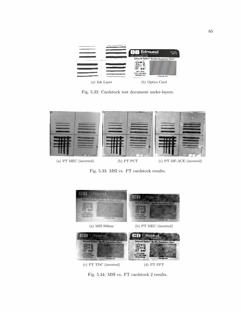
65

(a) Ink Layer (b) Optics Card

Fig. 5.32: Cardstock test document under-layers.

(a) PT MEC (inverted) (b) PT PCT (c) PT MF-ACE (inverted)

Fig. 5.33: MSI vs. PT cardstock results.

(a) MSI 950nm (b) PT MEC (inverted)

(c) PT TDC (inverted) (d) PT PPT

Fig. 5.34: MSI vs. FT cardstock 2 results.

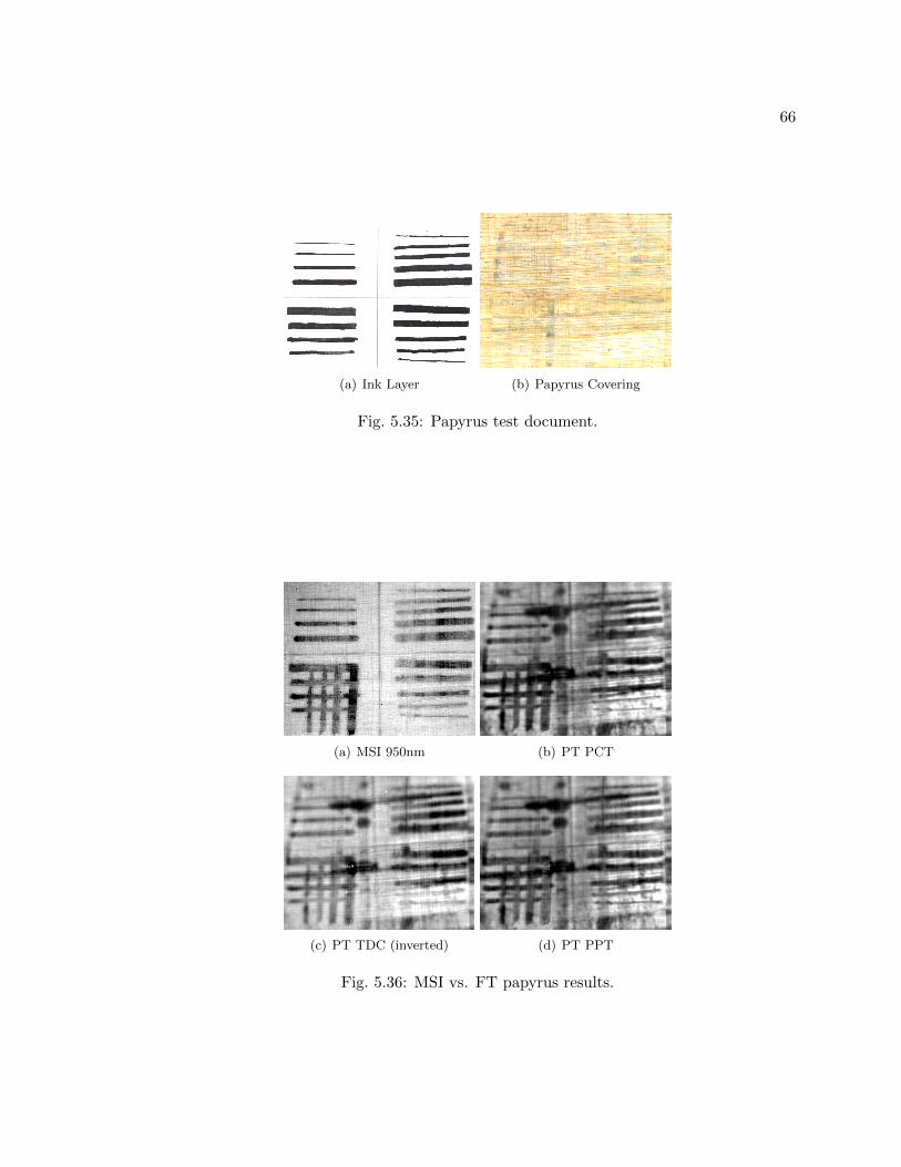
66

(a) Ink Layer (b) Papyrus Covering

Fig. 5.35: Papyrus test document.

(a) MSI 950nm (b) PT PCT

(c) PT TDC (inverted) (d) PT PPT

Fig. 5.36: MSI vs. FT papyrus results.

67

Figure 5.38. Both the MSI and the PT methods are able to reveal the majority of the ink

underneath the painted layer. However, the PT techniques are able to reveal the writings

beneath the black paint which the MSI fails to reveal. This indicates that PT can be used to

reveal writings underneath a layer that has similar spectral properties but different thermal

properties.

Figure 5.39 demonstrates the ability of flash thermography to reveal subsurface inks

beneath a layer of gesso. In this case, the MSI technique performs poorly. The results

presented in this section demonstrate the ability of flash thermography to image subsurface

inks beneath a variety of covering materials.

5.3.2 Document Strikeouts

For document strikeouts, MSI fails completely to reveal the under-layer of writing as

shown in Figure 5.40(a). However, Figures 5.40(b) and 5.40(c) prove the ability of flash

thermography to detect document strikeouts. The ability of flash thermography to detect

document strikeouts is a significant result that can allow for the evaluation of documents

that have previously been unable to analyze effectively.

5.3.3 Surface Writing Enhancement

The purpose of the test document shown in Figure 5.41(a) is to evaluate the ability

of flash thermography to enhance surface inks that have poor spectral contrast. Figures

5.41(b) and 5.41(c) show the results of two different wavelength MSI images. In the 950 nm

(a) Ink Layer (b) Paint Covering

Fig. 5.37: Paint test document.

68

(a) MSI 950nm (b) FT MEC

(c) FT THDp (d) FT PPT

Fig. 5.38: MSI vs. FT painted images.

(a) MSI 400nm (b) FT DAC

(c) FT PPT (d) FT Time-Difference Con-trast

Fig. 5.39: MSI vs. FT gesso images.

69

(a) MSI 950nm (b) PT MEC (inverted) (c) PT 2nd Derivative

Fig. 5.40: MSI vs. FT strikeout results.

image, the surface inks have poor contrast; however, in the 600 nm they have significant

contrast. The two ink writings can also be seen in the flash thermography images shown in

Figures 5.41(d)-5.41(f). Although both the red and blue inks can be seen in both MSI and

FT images, the important difference is the MSI images are comparing differences in optical

properties whereas the FT images are comparing the differences in thermal properties.

This indicates that flash thermography can be used to enhance the writings of surfaces

that contain poor spectral contrast but have a large differences in thermal properties of

materials.

5.4 Feasibility of Application to Archaeological Artifacts

The methodology presented in this thesis was validated by applying the developed flash

thermography techniques to a piece of Egyptian cartonnage and the Codex Selden.

5.4.1 Egyptian Cartonnage

The cartonnage is an ancient document with a complex structure, containing overlap-

ping areas of ink, papyrus, gesso, and paint. Further imaging challenges arise from the

significant material inhomogeneities and internal flaws contained within the cartonnage.

Figures 3.2 and 5.42 provides comparisons between standard imaging, MSI techniques, and

flash thermography techniques.

70

(a) Test Document (b) MSI 950nm (c) MSI 600nm

(d) PT PPT (e) PT 2nd Derivative (f) PT MF-ACE

Fig. 5.41: MSI vs. FT red surface results.

71

From these figures, several conclusions may be reached. First, both the MSI images

and the flash thermography images are comparable in their ability to significantly enhance

the cartonnage surface writing. The important difference between the two methods is the

technique used to enhance the surface writing. MSI enhances this text through differences

in the spectral characteristics of ink and the papyrus background. On the other hand, flash

thermography enhances the surface writing through differences in the thermal properties of

the ink and the papyrus background.

To illustrate that the ink is not enhanced due to spectral characteristics in flash ther-

mography, a pre-flash cartonnage image is shown in Figure 5.43. In the pre-flash image, the

surface ink cannot be observed, indicating that differences in spectral characteristics have

a insignificant contribution to the visualization of the ink. Thus text on ancient documents

that previously were not effectively imaged using MSI because of poor spectral contrast be-

tween inks and document backings, can now be imaged using flash thermography to reveal

these obscure writings.

A second important conclusion from this study is the improvement flash thermography

provides over MSI imaging when applied to ink just below the document structure. This

is illustrated in Figure 5.42(c). A red arrow points to a subsurface ink line that is not

observed in Figure 5.42(a). This indicates that flash thermography successfully revealed

shallow subsurface ink that MSI could not show.

5.4.2 Codex Selden

The Codex Selden is a Mesoamerican manuscript book that is a recognized palimpsest

[103–105]. The original pictograph drawings were covered with a gesso layer, and a new

set of pictographs were drawn on the surface. The Codex Selden presents several unique

imaging challenges including: (1) an unknown thickness of the gesso layer, (2) an unknown

extent to which the original writing has been removed, and (3) internal flaws within the

gesso that may obscure detectability of under-inks.

The Codex Selden data was collected using a ThermaCAM Phoenix 600 camera oper-

ating in the 1.5-5.0 µm range with a data acquistion rate of 67 frames/second. Two Sunpak

72

(a) MSI 950nm

(b) FT PPT Amplitude Image (Inverted)

(c) FT Standard Contrast

Fig. 5.42: MSI vs. FT cartonnage images.

73

Fig. 5.43: Pre-flash FT cartonnage image.

Pro System 622 flash units provided the impulse energy [106]. Imaging access to the Codex

Selden was limited and the images presented were obtained early in this research before the

most efficient flash thermography parameters had been established.

The results of imaging three sections of the Codex Selden are presented in Figures 5.44,

5.45, and 5.46. In Figure 5.46(b), the vertical and horizontal line discontinuities within the

image are an artifact of combining several images. Deeper document structural defects can

be detected using flash thermography techniques over MSI as illustrated by the examples

given. It is too premature to conclude if any of these areas are potentially subsurface inks.

In addition, flash thermography enhances the thin surface inks, demonstrating that ancient

inks as well as modern ink can be enhanced using flash thermography techniques. It is

reasonable to assume sufficient thermal bonding between the gesso and the subsurface inks.

Re-obtaining the data set with larger amplitude excitation pulse is recommended.

74

(a) Visible Image (b) MSI 1000 nm

(c) FT PPT (d) FT PCT

Fig. 5.44: MSI vs. FT Codex Selden images data set 1.

75

(a) Visible Image (b) MSI 750 nm

(c) FT PPT (d) FT MEC

Fig. 5.45: MSI vs. FT Codex Selden images data set 2.

76

(a) Visible Image (b) MSI 950nm

(c) FT PPT (d) FT MF t-statistic

Fig. 5.46: MSI vs. FT Codex Selden images data set 3.

77

Chapter 6

Conclusions and Recommendations

The conclusions developed from the results presented in Chapter 5 are summarized

in this chapter. The flash thermography parameters for effective flash thermography data

acquisition are outlined. A summary of methods for pre-processing, processing, and post-

processing the data to increase ink visualization are given. The ability of flash thermography

to image a variety of materials are discussed. Finally, this thesis concludes with recommen-

dations for future research.

6.1 Thermography Data Acquisition Parameters

Several flash thermography parameters were evaluated during the acquisition of the

data sets. Recommended values are discussed below.

Pulse Amplitude Four synchronized flash units were sufficient to reveal subsurface layers

of ink (after processing) through paper, card stock, papyrus, and thin gesso layers.

Large pulse amplitudes are desirable, but care must be taken to reduce the residual

heating from the flash bulb which may occur. For document strikeouts or enhancing

surface writing, a large pulse amplitude is unnecessary.

Pulse Duration Residual heating from flash pulse tails were not found to have a strong

negative effect on the detection process for deep-seated subsurface writings, provided

the tail decayed relatively quickly and absorbed uniformly into the document. For

document strikeouts and surface ink enhancement, a minimal input pulse length that

closely approximates an impulse is desired.

Sampling Frequency A sampling frequency of 87 Hz was found adequate for subsurface

defects; however, a faster sampling rate is recommended for document strikeouts and

surface ink enhancement.

78

Lens Filters The 3.42− 4.05 µm filter greatly outperformed the 2.65− 3.24 µm filter.

6.2 Pre-Processing

The following techniques were found useful for pre-processing flash thermography data

when applied in the following order:

1. Subtraction of a pre-flash image to each frame in order to reduce effects of non-uniform

surface emissivities;

2. A 3×3 pixel median filter applied to each frame for removing outliers caused by dead

pixels;

3. A 3×3 Gaussian low-pass filter, with a variance parameter of 0.8, applied to reduce

spatial image noise in each frame;

4. Thermal signal reconstruction (TSR), using a sixth order polynomial fitting, for re-

ducing temporal noise.

6.3 Processing

Effective processing techniques for each document class are presented. Table 6.1 out-

lines a rating system used in classifying the algorithms. Table 6.2 evaluates the pre-existing

and developed algorithm techniques used for processing flash thermography data of doc-

uments. Note that due to the similarities between processing strikeouts and surface ink

enhancement, the ratings for strikeouts also apply to surface writing enhancement.

6.4 Post-Processing

Essential post-processing methods include the following contrast stretching techniques:

1. Manual histogram manipulation,

2. Image normalization,

3. Image normalization with ends saturation,

79

Table 6.1: Algorithm rating system.

Value Definition Explanation

3 Highly RecommendedConsistently gives great results with minimalcomputational expense.

2 RecommendedPerforms well but inconsistently. May onlywork for simple document structures or com-putational expense is moderate.

1 Moderately RecommendedPerforms well occasionally or has a significantcomputation expense.

0 Not RecommendedEither fails to perform well or computationalexpense is prohibitive.

4. Pseudo-color images.

Other techniques which may be useful, depending on the situation, include:

1. Histogram equalization,

2. Image filter (median or Guassian),

3. Absolute and running contrast definitions.

6.5 Materials

This research demonstrated that flash thermography can be used to detect three types

of inks: carbon-based, iron gall, and modern ball-point. These inks were detected beneath

several covering layers including card stock, papyrus, paint, a gesso mix, and the ink itself.

6.6 Significant Contributions

This research resulted in the following significant contributions.

1. A comprehensive analysis of existing pulsed thermography processing techniques ap-

plied to documents, the magnitude of which does not exist in the literature. Pre-

existing techniques investigated include pseudo-color images, contrast stretching, syn-

thetic signal reconstruction, median and Gaussian low-pass filters, four contrast defi-

nitions, differential absolute contrast (DAC), derivative images, principal component

80

thermography (PCT), classical and reference-free implementations of dynamic thermal

tomography (DTT), pulse phase thermography (PPT), correlation images, transmis-

sion line matrix fitting algorithm (TLMFa), and pulsed thermography Hough trans-

form algorithm (PTHTa).

2. New pulsed thermography processing techniques that improve upon the results of the

existing techniques were developed. These techniques include Markov error contrast

(MEC), time-difference contrast, total harmonic distortion (THD), time constant anal-

ysis (TCA), and four matched filter definitions including spectral angle map (SAM),

adaptive coherence estimator (ACE), t-statistic, and F-statistic.

3. A proof-of-concept for detecting subsurface ink writings in documents.

4. Verification of the capability of pulsed thermography techniques to detect document

strikeouts.

5. Demonstrates the ability to enhance surface writings based on differences in thermal

characteristics when spectral characteristics do not differ significantly.

6. Demonstrates that pulsed thermography significantly improves upon multi-spectral

imaging for subsurface and surface writing enhancement.

7. Provides an evaluation of flash thermography parameters for the most effective doc-

ument imaging.

8. Validates the findings presented through application of flash thermography techniques

to a piece of Egyptian cartonnage and the Codex Selden.

9. A Pulsed Thermography Toolbox was developed providing a graphical user interface in

MATLAB for the straight-forward application of the presented processing techniques

to flash thermography data.

81

6.7 Recommendations for Future Research

There are two principal directions suggested for future research. The first recommen-

dation is the development of advanced thermal models that account for the uneven, multiple

layers which are often found in ancient documents. From these advanced thermal models,

processing techniques with greater effectiveness can be developed specific to this applica-

tion. The second recommendation is research into alternate heating methods to facilitate

for greater excitation energy. Methods of future research could explore step heating, ther-

mal transfer heating, or modulated thermography techniques. For document strikeouts,

it is recommended that the experiments be repeated using a thermal camera capable of

significantly faster frame rates. Investigation of techniques which account for the lateral

diffusion through the ink would also be beneficial.

82

Tab

le6.

2:P

roce

ssin

gal

gori

thm

ssu

mm

ariz

ed.

Pro

cess

ing

Tec

hn

iqu

eS

ub

surf

ace

Rati

ng

Str

ikeo

ut

Rati

ng

Wall

Tim

e(S

ec)

Com

men

ts

Con

tras

tD

efinit

ion

s1

10.0

3951

Can

be

use

das

ap

ost

-pro

cess

or.

(4.2

.6)

Diff

eren

tial

Abso

lute

Con

tras

t(D

AC

)3

30.0

3191

Req

uir

esp

ara

met

erse

lect

ion

.(4

.2.7

)

Der

ivat

ive

Imag

es2

34.0

37

Use

lim

ited

tim

ese

qu

ence

for

stri

keou

ts.

(4.2

.8)

Pri

nci

pal

Com

pon

ent

Ther

mog

raphy

(PC

T)

22

0.7

850

May

enh

an

ceso

me

featu

res

over

oth

ers.

Use

lim

ited

tim

ese

qu

ence

for

stri

keo

uts

.(4

.2.9

)

Cla

ssic

alD

yn

amic

Th

erm

alT

omog

rap

hy

(DT

T)

12

2.9

48

Per

form

sm

od

erate

lyfo

rd

etec

tin

gst

rike

ou

ts.

(4.2

.10)

Ref

eren

ce-f

ree

Dyn

amic

Th

erm

alT

omog

raphy

(DT

T)

21

6.8

43

Un

ab

leto

reve

al

the

dee

pes

td

efec

tsan

dh

as

am

od

erate

com

pu

tati

on

al

load

.(4

.2.1

0)

Pu

lsed

Ph

ase

Th

erm

ogra

phy

(PP

T)

33

0.3

465

Con

sist

entl

yp

erfo

rms

wel

l.(4

.2.1

1)

Cor

rela

tion

Imag

es0

010.7

6G

ener

all

yp

oor

per

form

an

ce.

(4.2

.12)

Tra

nsm

issi

onL

ine

Mat

rix

Fit

ting

(TL

MF

a)0

04044

Pro

hib

itiv

ely

larg

eco

mp

uta

tional

exp

ense

.(4

.2.1

3)

PT

Hou

ghT

ran

sfor

m(P

TH

Ta)

10

125.9

Larg

eco

mp

uta

tion

al

exp

ense

.(4

.2.1

4)

Tim

e-D

iffer

ence

Con

tras

t(T

DC

)3

31.3

57

Diff

eren

cin

gea

chfr

am

efr

om

the

fift

hp

revi-

ou

sis

effec

tive

.(4

.3.1

)

Tot

alH

arm

onic

Dis

tort

ion

(TH

D)

22

0.3

365

Work

sb

est

wit

hsi

mp

led

ocu

men

tst

ruct

ure

s.(4

.3.2

)

Mar

kov

Err

orC

ontr

ast

(ME

C)

33

0.1

597

Per

form

sco

nsi

sten

tly

wel

l.(4

.3.3

)

Tim

eC

onst

ant

An

alysi

s(T

CA

)1

199.9

6L

imit

edto

sim

ple

docu

men

tsan

dh

as

ala

rge

com

pu

tati

on

al

exp

ense

.(4

.3.4

)

Mat

ched

Filte

rs(S

AM

,A

CE

,t/

F-s

tati

stic

)3

31.0

75

Req

uir

esp

rop

erse

lect

ion

of

dee

pes

td

efec

tare

a.

(4.3

.5)

83

References

[1] F. C. Sham, N. Chen, and L. Long, “Surface crack detection by flash thermographyon concrete surface,” Insight, vol. 50, no. 5, pp. 240–243, April 2008.

[2] J. Sham Fung Chu, Studies of Using Infrared Flash Thermography (FT) for Detec-tion of Surface Cracks, Subsurface Defects and Water-Paths in Building ConcreteStructures. Ph.D. dissertation, City University of Hong Kong, July 2008.

[3] H. Nayeb-Hashemi, D. Swet, and A. Vaziri, “New electrical potential method formeasuring crack growth in nonconducive materials,” Measurements, vol. 36, pp. 121–129, 2004.

[4] M. A. Omar, Y. Zhou, R. Parvataneni, and E. Planting, “Calibrated pulse-thermography procedure for inspecting HDPE,” Research Letters in Materials Sci-ence, vol. 2008, no. 186427, p. 4, 2008.

[5] K. T. Wan and C. K. Y. Leung, “Fiber optics sensor for the monitoring of mixedmode cracks in structures,” Sensors and Actuators, vol. 135, pp. 370–380, 2007.

[6] C. Ibarra-Castanedo, M. Genest, P. Servais, X. P. V. Maldague, and A. Bendada,“Qualitative and quantitative assessment of aerospace structures by pulsed thermog-raphy,” Nondestructive Testing and Evaluation, vol. 22, no. 2-3, pp. 199–215, June-September 2007.

[7] P. Meinlschmidt, “Thermographic detection of defects in wood and wood-based mate-rials,” 14th International Symposium of Nondestructive Testing of Wood, May 2005.

[8] M. Y. Y. Hung, Y. S. Chen, S. P. Ng, S. M. Shepard, Y. Hou, and J. R. Lhota,“Review and comparison of shearography and pulsed thermography for adhesivebond evaluation,” Optical Engineering, vol. 46, no. 5, p. 051007, 2007 [Online].Available: http://link.aip.org/link/?JOE/46/051007/1.

[9] J. A. Schroeder, T. Ahmed, B. Chaudhry, and S. Shepard, “Non-destructivetesting of structural composites and adhesively bonded composite joints: pulsedthermography,” Composites Part A: Applied Science and Manufacturing, vol. 33,no. 11, pp. 1511–1517, 2002 [Online]. Available: http://www.sciencedirect.com/

science/article/B6TWN-47YXF1T-6/2/bc71b40b35ddc50e5ea83126db42480d.

[10] D. A. Scott, M. Dennis, N. Khandekar, J. Keeney, D. Carson, and L. S. Dodd, “AnEgyptian cartonnage of the Graeco-Roman period: examination and discoveries,”Studies in Conservation, vol. 48, no. 1, pp. 41–56, 2003.

[11] D. Bomford, Art in the Making: Underdrawings in Renaissance Paintings, ser. Na-tional Gallery London Publications. New Haven: Yale University Press, 2002.

84

[12] B. Berrie, E. R. de la Rie, R. Hoffman, J. Tomlinson, T. Wiesel, and J. Winter,Scientific Examination of Art: Modern Techniques in Conservation and Analysis.Washingtion DC: National Academy of Sciences, 2002.

[13] L. MacDonald, Digital Heritage: Applying Digital Imaging to Cultural Heritage. Am-sterdam: Elsevier, 2006.

[14] C. M. Falco, “High resolution digital camera for infrared reflectography,” Review ofScientific Instruments, vol. 80, no. 7, pp. 071 301–071 309, July 2009.

[15] A. H. Bendada, S. Sfarra, D. Ambrosini, D. Paoletti, C. Ibarra-Castanedo, andX. Maldague, “Active thermography data processing for the NDT&E of frescoes,” inQuantitative Infrared Thermography 2010, pp. 961–966, Quebec City, Canada, July2010.

[16] G. M. Carlomagno and C. Meola, “Comparison between thermographic techniquesfor frescoes NDT,” NDT & E International, vol. 35, no. 8, pp. 559–565, 2002.

[17] K. Blessley, C. Young, J. Nunn, J. Coddington, and S. M. Shepard, “The feasibilityof flash thermography for the examination and conservation of works of art,” Studiesin Conservation, vol. 55, pp. 107–120, 2010.

[18] D. Gavrilov, C. Ibarra-Castanedo, E. Maeva, O. Grube, X. Maldague, and R. Maev,“Infrared methods in noninvasive inspection of artwork,” 9th International Conferenceon Non-destructive Testing of Art, 2008.

[19] C. Ibarra-Castanedo, S. Sfarra, D. Ambrosini, D. Paoletti, A. Bendada, andX. Maldague, “Subsurface defect characterization in artworks by quantitative PPT,”Quantitative Infrared Thermography, 2008.

[20] D. Ambrosini, C. Daffara, R. D. Biase, D. Paoletti, L. Pezzati, R. Bellucci, and F. Bet-tini, “Integrated reflectography and thermography for wooden paintings diagnostics,”Journal of Cultural Heritage, vol. 11, no. 2, pp. 196–204, 2010.

[21] M. Lettner and R. Sablatnig, “Multispectral imaging for analyzing ancientmanuscripts,” 17th European Signal Processing Conference, August 2009.

[22] K. Rapantzikos and C. Balas, “Hyperspectral imaging: potential in non-destructiveanalysis of palimpsests,” in IEEE International Conference on Image Processing,vol. 2, pp. II–618–21, Sept. 2005.

[23] G. A. Ware, D. M. Chabries, and R. W. Christiansen, “Multispectral document en-hancement: Ancient carbonized scrolls,” IEEE Proceedings on Geoscience and RemoteSensing Symposium, pp. 2486–2488, 2000.

[24] R. J. Easton, K. Knox, and W. Christens-Barry, “Multispectral imaging of theArchimedes palimpsest,” in Applied Imagery Pattern Recognition Workshop, pp. 111–116, Oct. 2003.

[25] D. Obbink, “A new Archilochus poem,” Zeitschrift fur Papyrologie und Epigraphik,vol. 156, pp. 1–9, 2006.

85

[26] B. Zuckerman, “Bringing the Dead Sea scrolls back to life: A new evaluation ofphotographic and electric imaging of the Dead Sea scrolls,” Dead Sea Discoveries,vol. 3, no. 2, pp. 178–207, 1996.

[27] G. Bearman, B. Zuckerman, K. Zuckerman, and J. Chiu, “Multi-spectral digital imag-ing of Dead Sea scrolls and other ancient documents,” Jet Propulsion Laboratory,Tech. Rep., 1993.

[28] J. Monaghan, G. Ware, J. Pohl, and S. Houston, “A codex imaging project at theBodleian library: the recovery of lost mixtec writing,” Foundation for the Advance-ment of Meso-American Studies, 2004.

[29] U. Bergmann and K. T. Knox, “Pseudo-color enhanced X-ray fluorescence imaging ofthe Archimedes Palimpsest,” Proceedings Document Recognition and Retrieval, vol.XVI, pp. 1–10, Jan. 2009.

[30] X. P. Maldague, Theory and Practice of Infrared Technology for Nondestructive Test-ing. Hoboken: John Wiley & Sons, Inc., 2001.

[31] R. C. Gonzalez and R. E. Woods, Digital Image Processing. Upper Saddle River:Pearson Education, Inc., 2008.

[32] J. Zalameda, N. Rajic, and W. Winfree, “A comparison of image processing algorithmsfor thermal nondestructive evaluation,” SPIE Proc. Thermosense XXV, vol. 5073, pp.374–385, 2003.

[33] C. Ibarra-Castanedo, D. Gonzalez, M. Klein, M. Pilla, S. Vallerand, and X. Maldague,“Infrared image processing and data analysis,” Infrared Physics & Technology, vol. 46,pp. 75–83, Apr. 2004.

[34] J. Ramirez-Granados, G. Paez, and M. Strojnik, “Reconstruction and analysis ofpulsed thermographic sequences for nondestructive testing of layered materials,” Ap-plied Optics, vol. 49, no. 9, Mar. 2010.

[35] S. Shepard, J. Lhota, B. Rubadeux, T. Ahmed, and D. Wang, “Enhancement andreconstruction of thermographic data,” Proceedings SPIE, vol. 4710, pp. 531–535,2002.

[36] S. M. Shepard, “Temporal noise reduction, compression and analysis ofthermographic image data sequences,” Patent, 02 2003, uS 6516084 [Online].Available: http://www.patentlens.net/patentlens/patent/US_6516084/en/.

[37] M. Pilla, M. Klein, X. Maldague, and A. Salerno, “New absolute contrast for pulsedthermography,” Proceedings of Quantitative Flash Thermography, pp. 53–58, 2002.

[38] D. Gonzalez, C. Ibarra-Castanedo, M. Pilla, M. Klein, and X. Maldague, “Automateddifferential absolute contrast,” Quantitative Infrared Thermography, 2004.

[39] M. Susa, H. Benitez, C. Ibarra-Castanedo, H. Loaiza, H. Bendada, and X. Maldague,“Phase contrast using a differentiated absolute contrast method,” Quantitative In-frared Thermography, vol. 3, pp. 219–230, 2006.

86

[40] D. Gonzalez, C. Ibarra-Castanedo, M. Pilla, M. Klein, J. Lopez-Higuera, andX. Maldague, “Automatic interpolated differentiated absolute contrast algorithm forthe analysis of pulsed thermographic sequences,” in Quantitative Infrared Thermogra-phy 7, D. Balageas, J. Buchlin, G. Carlomagno, and G. Busse, Eds., pp. H.16.1–H.16.6,Bruxelles, Belgique, July 2004.

[41] H. Benitez, C. Ibarra-Castanedo, A. Bendada, X. Maldague, H. Loaiza, andE. Caicedo, “Definition of a new thermal contrast and pulse correction for defectquantification in pulsed thermography,” Infrared Physics & Technology, vol. 51, pp.160–167, 2008.

[42] C. Ibarra-Castanedo, H. Benitez, X. Maldague, and A. Bendada, “Review of thermal-contrast-based signal processing techniques for the nondestructive testing and eval-uation of materials by infrared thermography,” International Workshop on ImagingNondestructive Evaluation, 07.

[43] H. Benitez, X. Maldague, C. Ibarra-Castanedo, H. Loaiza, A. Bendada, andE. Caicedo, “Modified differential absolute contrast using thermal quadrupoles forthe nondestructive testing of finite thickness specimens by infrared thermography,” inElectrical and Computer Engineering, 2006. CCECE ’06. Canadian Conference on,pp. 1039–1042, may 2006.

[44] X. Maldague and S. Marinetti, “Pulse phase infrared thermography,” Journal of Ap-plied Physics, vol. 79, no. 5, pp. 2694–2698, mar 1996.

[45] M. A. Omar and Y. Zhou, “A quantitative review of three flash thermographyprocessing routines,” Infrared Physics & Technology, vol. 51, no. 4, pp. 300–306, 2008 [Online]. Available: http://www.sciencedirect.com/science/article/

B6TJ9-4R0643G-2/2/1012d8792b0b432e3dfd2514330f125c.

[46] G. Busse, D. Wu, and W. Karpen, “Thermal wave imaging with phase sensitivemodulated thermography,” Journal of Applied Physics, vol. 71, no. 8, pp. 3962–3965,apr 1992.

[47] X. Maldague, F. Galmiche, and A. Ziadi, “Advances in pulsed phase thermography,”Infrared Physics & Technology, vol. 43, pp. 175–181, 2002.

[48] C. Ibarra-Castanedo and X. Maldague, “Defect depth retrieval from pulsed phasethermographic data on plexiglas and aluminum samples,” SPIE Proc. ThermosenseXXVI, vol. 5405, 2004.

[49] D. Gonzalez, C. Ibarra-Castanedo, F. Madruga, and X. Maldague, “Differentiatedabsolute phase contrast algorithm for the analysis of pulsed thermographic sequences,”Infrared Physics & Technology, vol. 48, pp. 16–21, 2006.

[50] M. Klein, A. Bendada, C. Ibarra-Castanedo, and X. Maldague, “A hybrid pulsedthermography processing technique for the depth estimation of subsurface defectscombining TSR and PPT,” 10th International Conference on Quantitative InfraredThermography, 2010.

87

[51] S. M. Shepard. (2007, October) Flash thermography of aerospace composites[Online]. Available: http://www.ndt.net/article/panndt2007/papers/132.pdf.

[52] S. M. Shepard, J. R. Lhota, B. A. Rubadeux, D. Wang, and T. Ahmed, “Reconstruc-tion and enhancement of active thermographic image sequences,” Optical Engineering,vol. 42, no. 5, May 2003.

[53] J. G. Sun, “Analysis of pulsed thermography methods for defect depth prediction,”Journal of Heat Transfer, vol. 128, no. 4, pp. 329–338, 2006.

[54] S. M. Shepard, “Understanding flash thermography,” Materials Evaluation, pp. 460–464, May 2006.

[55] S. M. Shepard, J. Hou, J. R. Lhota, and J. M. Golden, “Automated processing ofthermographic deriviatives for quality assurance,” Optical Engineering, vol. 46, no. 5,May 2007.

[56] N. Rajic, “Principal component thermography for flaw contrast enhancement andflaw depth characterisation in composite structures,” Composite Structures, vol. 58,no. 4, pp. 521–528, 2002 [Online]. Available: http://www.sciencedirect.com/

science/article/B6TWP-472841H-9/2/4c29e1491d0beb293d9a3811ed9498b8.

[57] N. Rajic, “Principal component thermography,” Defense Science and TechnologyOrganisation Victoria (Australia) Aeronautical and Maritime Research Laboratory,Tech. Rep. 012-294, Apr. 2002.

[58] V. Vavilov, D. Nesteruk, V. Shiryaev, A. Ivanov, and W. Swiderski, “Thermal (in-frared) tomography: terminology, principal procedures, and application to nonde-structive testing of composite materials,” Russian Journal of Nondestructive Testing,vol. 46, no. 3, pp. 151–161, 2010.

[59] V. P. Vavilov, “Dynamic thermal tomography: perspective field of thermal NDT,”S. A. Semanovich, Ed., vol. 1313, no. 1, pp. 178–182. SPIE, 1990 [Online]. Available:http://link.aip.org/link/?PSI/1313/178/1.

[60] W. Swiderski, “The characterization of defects in multi-layered composite materialsby thermal tomography methods,” in Proceedings of the Tenth Annual Conference ofthe Materials Research Society of Serbia, vol. 115, no. 4, pp. 800–804, 2009.

[61] B. Sun, Q. Ma, and H. Zhao, “Fitting-correlation analysis of pulsed thermographicsequence data,” in Proceedings of the 2007 IEEE International Conference on Mecha-tronics and Automation, Aug. 2007.

[62] M. Klein, C. Ibarra-Castanedo, A. H. Bendada, and X. Maldague, “Thermographicsignal processing through correlation operators in pulsed thermography,” in Ther-mosense XXX, SPIE Defense and Security Symposium, V. P. Vavilov and D. D.Burleigh, Eds., vol. 6939, p. 693915, Orlando, Florida, USA, Vol. 6939, March 16-202008.

88

[63] D. Gonzalez, C. Ibarra-Castanedo, J. Lopez-Higuera, and X. Maldague, “New algo-rithm based on the Hough transform for the anlaysis of pulsed thermographic se-quences,” Nondestructive Testing and Evaluation International, vol. 39, pp. 617–621,2006.

[64] C. Ibarra-Castanedo, D. Gonzalez, F. Galmiche, X. Maldague, and A. H. Bendada,“Discrete signal transforms as a tool for processing and analyzing pulsed thermo-graphic data,” in SPIE - The International Society for Optical Engineering, Ther-mosense XXVIII, vol. 6205, pp. 620 514–1–620 514–12, Orlando, FL, 2006.

[65] D. de Cogan, A. Soulos, and K. Chichlowski, “Sub-surface feature location and identi-fication using inverse TLM techniques,” Microelectronics Journal, vol. 29, pp. 215–22,1998.

[66] D. de Cogan, W. J. O’Connor, and S. Pulko, Transmission Line Matrix in Computa-tional Mechanics. Boca Raton: Taylor and Francis, 2006.

[67] D. Crowther, L. Favro, P. Kuo, and R. Thomas, “Inverse scattering algorithm appliedto infrared thermal waves,” J. Appl. Phys., vol. 74, no. 9, pp. 5828–5835, Nov 1993.

[68] Favro, L. D., Han, X., Kuo, P. K., and Thomas, R. L., “Improving the resolution ofpulsed thermal wave images with a simple inverse scattering technique,” Journal DePhysique IV France, vol. 04, pp. C7–545–C7–550, 1994.

[69] L. Favro, D. Crowther, P. Kuo, and R. Thomas, “Inversion of pulsed thermal-waveimages for defect sizing and shape recovery,” Thermosense XIV: An InternationalConference on Thermal Sensing and Imaging Diagnostic Applications, vol. 1682, pp.178–181, 1992.

[70] N. S. Goel and F. Gang, “A simple method for pulse-echo thermal wave imagingof arbitrary shaped subsurface scatterers in heterogeneous materials,” InternationalCommunications in Heat Mass Transfer, vol. 23, no. 1, pp. 45–54, 1996.

[71] R. Thomas, L. Favro, and P. Kuo, “Thermal wave imaging of hidden corrosion,”Wayne State University, Tech. Rep. F49620-96-1-0166, Mar. 1998.

[72] M. Omar, H. Hassan, and K. Saito, “Optimizing thermography depth probing with adynamic thermal point spread function,” Infrared Physics & Technology, vol. 46, pp.506–514, 2005.

[73] T. D’Orazio, C. Guaragnella, M. Leo, and P. Spagnolo, “Defect detection in aircraftcomposites by using a nerual appoach in the analysis of thermographic sequences,”Nondestructive Testing and Evaluation International, vol. 38, pp. 665–673, 2005.

[74] D. Maillet, J. Batsale, A. Bendada, and A. Degiovanni, “Methodes integrales et con-trole non destructif par thermographie infrarouge,” Revue Generale de Thermique,vol. 35, pp. 14–27, 1996.

[75] A. Bendada, F. Erchiqui, and M. Lamontagne, “Pulsed thermography in the evalu-ation of an aircraft composite using 3D thermal quadrupoles and mathematical per-turbations,” Inverse Problems, vol. 21, pp. 857–577, 2005.

89

[76] V. Vavilov, IR Thermography and Nondestructive Testing. Moscow: Spektr, 2009.

[77] J. Sun, “Method for determining defect depth using thermal imaging,” Patent, 042002, US 6542849.

[78] N. Rajic, “A quantitative approach to active thermographic inspection for materialloss evaluation in metallic structures,” Research in Nondestructive Evaluation, vol. 12,no. 2, pp. 119–131, 2000.

[79] V. Vavilov, X. Maldague, B. Dufort, and A. Ivanov, “Adaptive thermal tomographyalgorithm,” Proceedings SPIE Thermosense-XV, no. 1933, pp. 166–173, 1993.

[80] H. Benitez, H. Loaiza, E. Caicedo, C. Ibarra-Castanedo, A. Bendada, andX. Maldague, “Defect characterization in infrared non-destructive testing with learn-ing machines,” Nondestructive Testing & Evaluation International, vol. 42, pp. 630–643, 2009.

[81] I. Abdel-Qader, S. Yohali, O. Abudayyeh, and S. Yehia, “Segmentation of thermal im-ages for non-destructive evaluation of bridge decks,” Nondestructive Testing & Eval-uation International, vol. 41, no. 5, pp. 395–405, 2008.

[82] V. F. Bakirov, R. A. Kline, and W. P. Winfree, “Multiparameter thermal tomogra-phy,” AIP Conference Proceedings, vol. 700, no. 1, pp. 461–468, 2004.

[83] V. Bakirov, R. Kline, and W. Winfree, “Diffusion based thermal tomography,” Non-destructive Evaluation and Reliability of Micro and Nonomaterial Systems, vol. 4703,pp. 219–225, 2002.

[84] V. F. Bakirov and R. A. Kline, “Diffusion-based thermal tomography,” Journal ofHeat Transfer, vol. 127, no. 11, pp. 1276–1279, 2005.

[85] F. Ammirato and P. Zayicek, “Infrared thermography field application guide,” ElectricPower Research Institute, Inc., Palo Alto, CA, Tech. Rep. TR-107142, Jan. 1999.

[86] M. Klein, C. Ibarra-Castanedo, X. Maldague, and A. H. Bendada, “IR-View: astraightforward graphical user interface for basic and advanced signal processing ofthermographic infrared sequences,” in Thermosense XXX, SPIE Defense and SecuritySymposium, V. P. Vavilov and D. D. Burleigh, Eds., vol. 6939, p. 693914, Orlando,Florida, USA, Vol. 6939, March 16-20 2008.

[87] S. Shepard, J. Lhota, and T. Ahmed, “Flash thermography contrast model based onIR camera noise characteristics,” Nondestructive Testing and Evaluation, vol. 22, no.2-3, pp. 113–126, 2007.

[88] V. Vavilov, “Pulsed thermal NDT of materials: back to the basics,” NondestructiveTesting and Evaluation, vol. 22, no. 2-3, pp. 177–197, June 2007.

[89] P. Zayicek, “Infrared thermography guide (revision 3),” Electric Power Research In-stitute, Inc., Tech. Rep. 1006534, 2002.

90

[90] X. Maldague, Nondestructive Evaluation of Materials by Infrared Thermography.London: Springer-Verlag, 1993.

[91] J. Krapez, D. Balegeas, A. Deom, and F. Lepoutre, “Early detection by stimulated in-frared thermography,” in Advances in Signal Processing for Nondestructive Evaluationof Materials, X. Maldague, Ed., pp. 303–321. The Netherlands: Kluwer AcademicPublished, 1994.

[92] J. R. Lhota and S. M. Shepard, “Critical timing issues in flash thermography,” D. O.Thompson and D. E. Chimenti, Eds., vol. 760, no. 1, pp. 1654–1660. AIP, 2005[Online]. Available: http://link.aip.org/link/?APC/760/1654/1.

[93] U. Netzelmann, “Optimized temporal excitation profiles in active thermography,”Analytical Sciences, vol. 17, pp. 432–435, Apr. 2001.

[94] X. Maldague, Z. Ziadi, and M. Klein, “Double pulse infrared thermography,” Nonde-structive Testing and Eval. Int., vol. 37, pp. 559–564, 2004.

[95] A. Daniels, “Optimization of pulsed temporal stimulation for thermal nondestructivetesting,” in Thermosense XX SPIE, J. Snell and R. Wurzbach, Eds., vol. 3361, pp.254–265, 2001.

[96] H. Carslaw and J. Jaeger, Conduction of Heat in Solids, 2nd ed. Oxford: ClaredonPress, 1986.

[97] K. Wan and Q. Ma, “Data-fitting reconstruction for defect inspection of airplanealuminum structure in infrared thermographic NDT,” in Industrial Electronics andApplications, 2009. ICIEA 2009. 4th IEEE Conference on, pp. 691–696, may 2009.

[98] H. Ringermacher, D. Mayton, D. Howard, and B. Cassenti, “Towards a flat-bottomhole standard for thermal imaging,” Review of Progress in Quantitative Nondestruc-tive Evaluation, vol. 17, pp. 425–9, 1998.

[99] M. Omar, M. Hassan, K. Saito, and R. Alloo, “IR self-referencing thermography fordetection of in-depth defects,” Infrared Physics & Technology, vol. 46, pp. 283–289,2005.

[100] T. A. Griffiths, “Enhancing multispectral imagery of ancient documents,” Master’sthesis, Utah State University, 2011.

[101] B. Foy, “Overview of target detection algorithms for hyperspectral data,” Los AlamosNational Laboratory, Tech. Rep. LA-UR-09-00593, June 2009.

[102] D. Manolakis, “Taxonomy of detection algorithms for hyperspectral imaging applica-tions,” Optical Engineering, vol. 44, no. 6, pp. 066 403–1–066 403–11, June 2005.

[103] M. E. Smith, “Codex selden: A manuscript from the Valley of Nochixlan,” in TheCloud People: Divergent evolution of the Zapotec and Mixtec civilizations, K. Flanneryand J. Marcus, Eds., pp. 248–255. New York: Academic Press, 1984.

91

[104] M. E. Smith, “Why the second Codex Selden was painted,” in Caciques and theirpeople, J. Marcus and J. F. Zeitlin, Eds., vol. 89, pp. 111–142. AnthropologicalPapers, 1994.

[105] P. Dark and J. Plesters, “The palimpsests of Codex Selden: Recent attempts to revealthe covered pictographs,” 33rd Annual International Congress of Americanists, vol. 2,pp. 530–539, 1958.

[106] G. A. Ware, “Codex selden feasibility study: multispectral and infrared images,”Brigham Young University, Tech. Rep., 2005.

92

Appendices

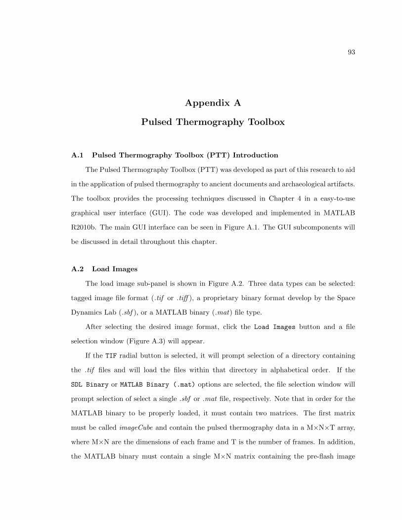
93

Appendix A

Pulsed Thermography Toolbox

A.1 Pulsed Thermography Toolbox (PTT) Introduction

The Pulsed Thermography Toolbox (PTT) was developed as part of this research to aid

in the application of pulsed thermography to ancient documents and archaeological artifacts.

The toolbox provides the processing techniques discussed in Chapter 4 in a easy-to-use

graphical user interface (GUI). The code was developed and implemented in MATLAB

R2010b. The main GUI interface can be seen in Figure A.1. The GUI subcomponents will

be discussed in detail throughout this chapter.

A.2 Load Images

The load image sub-panel is shown in Figure A.2. Three data types can be selected:

tagged image file format (.tif or .tiff ), a proprietary binary format develop by the Space

Dynamics Lab (.sbf ), or a MATLAB binary (.mat) file type.

After selecting the desired image format, click the Load Images button and a file

selection window (Figure A.3) will appear.

If the TIF radial button is selected, it will prompt selection of a directory containing

the .tif files and will load the files within that directory in alphabetical order. If the

SDL Binary or MATLAB Binary (.mat) options are selected, the file selection window will

prompt selection of select a single .sbf or .mat file, respectively. Note that in order for the

MATLAB binary to be properly loaded, it must contain two matrices. The first matrix

must be called imageCube and contain the pulsed thermography data in a M×N×T array,

where M×N are the dimensions of each frame and T is the number of frames. In addition,

the MATLAB binary must contain a single M×N matrix containing the pre-flash image

94

Fig. A.1: Pulsed Thermography Toolbox main GUI.

Fig. A.2: Load images panel.

Fig. A.3: Select files interface.

95

with the variable name preflash. After the data are loaded, the first image of the data set

will be shown on the Display Panel (Figure A.4).

The Display Panel features a slider that controls which frame is currently displayed.

The Play All button iterates through every frame showing the video sequence. Finally,

the image number is displayed in the upper left, and the image tag information is displayed

in the upper right.

A.3 Manually Manipulate Data Panel

The Manually Manipulate Data Panel is shown in Figure A.5 and provides a variety

of features for exploring and manipulating the data manually. The Explore Data button

brings up the Explore Data Sub-GUI as discussed in Section A.8.

The Crop Images button allows each frame in the data set to be cropped. After clicking

the Crop Images button, the image corresponding to the number in the FlashPoint edit

box will be displayed allowing selection of a rectangular region on the image displayed in

the Display Panel. After selecting the region to keep, right-click on the image and select

the Crop Image item from the drop-down menu. Each image frame will be cropped to the

specified dimensions.

The Select Colormap drop-down box allows the user to select the colormap to be

used in creating the false color images (see Section 4.2.1). To view the original grayscale

intensity images, select the Grayscale option from the drop-down box.

The FlashPoint and RemoveEnd edit boxes are initialized with the length of the data.

These boxes allow for the data set to be reduced in length. Changing the number in the

FlashPoint edit box allows removal of any images before that point (pre-flash images).

By changing the number in the RemoveEnd edit box, the total number of frames can be

reduced. After entering the desired parameters, press the Remove Images button to apply

the actions. Note that when changing the Flashpoint, the third previous image will be

saved as the pre-flash image used for future calculations. Finally, the Est. FlashPoint

button can be used to automatically detect the flash point, give an estimation of the length

96

Fig. A.4: Display panel.

Fig. A.5: Manually Manipulate Data Panel.

97

of data needed, and update these values in the FlashPoint and RemoveEnd edit boxes,

respectively.

A.4 Pre-Processing Panel

The Pre-Processing Panel, shown in Figure A.6, provides useful pre-processing routines.

Recommended settings are pre-selected. The Remove Surface Effusivities subtracts

the pre-flash image from each image in the data set to reduce the effects of differences in

surface effusivity values. The Spatial Noise Reduction selects the image filters discussed

in Section 4.2.4. Both the filters use a 3×3 window. The variance of the Gaussian filter,

which affects the amount of blurring, can be changed using the slider box labeled Variance.

The Normalize Cube checkbox allows for the entire data set to be re-normalized between 0

and 1. This is useful when the data set does not fill the entire range due to the median filter

removing dead pixels or other abnormalities. Finally, the Signal Reconstruction provides

a choice between the synthetic signal reconstruction techniques discussed in Section 4.2.5.

When Layered Reconstruction is selected, the number of layers to use in reconstruction

can be changed using the Num. Layers slider. In addition, the reconstructed signal can

be modified using the Interpolation edit box. An interpolation factor of 2 will up-sample

the signal by double. Similarly, an interpolation factor of 0.5 will down-sample the signal

by one half. When all the chosen pre-processing techniques have been selected, click the

Pre-Process button to apply them to the data set.

Fig. A.6: Pre-Processing Panel.

98

A.5 Processing Panel

The Processing Panel is shown in Figure A.7 and allows for the operator to choose

a desired processing algorithm as discussed in Chapter 4. When the desired algorithm is

chosen, click the Process button to apply the algorithm to the data set. One of the options

in the drop-down box is ### Sandbox ###. When this option is selected, the Sandbox

drop-down menu is enabled. This drop-down menu is automatically populated with any

functions located in the sandbox/ directory. Choose any of the functions in the sandbox

drop-down menu and click Process to run the selected algorithm. Note that any algorithm

placed in the sandbox/ directory is required to have a standard header with a single input

and two outputs. The input is an image cube of the input data with dimensions M×N×T.

The outputs are a processed data cube M×N×R and a cell array of string image descriptors

of length R. This facilitates straightforward testing of new processing routines which can

be easily incorporated into the existing GUI.

A.6 Post-Processing Panel

The Post-Processing Panel is seen in Figure A.8 and provides the three contrast stretch-

ing routines discussed in Sections 4.2.2 and 4.2.3. After selecting the desired post-processing

technique, click Post-Process button to apply to the data set.

A.7 Other GUI Sub-Components

There are several other GUI sub-components. The Which Cube panel allows for the

selection between data sets at different stages of processing. The Enable Multicore

Processing makes it possible for MATLAB to use four processors when processing the

Fig. A.7: Processing Panel.

99

Fig. A.8: Post-Processing Panel.

data. The Adjust Contrast button displays the histogram of the currently displayed im-

age frame and allows for manual histogram manipulation. The Open IR View passes the

data to the IR View toolbox, a previously existing open-source toolbox for processing ther-

mal data. Note that the IR View toolbox was made for a previous version of MATLAB

and not all of the functions work correctly. The Write To File outputs the currently se-

lected data to file in the results/[algorithm name]/ directory in .tif format. The filenames

are generated from the image tag cell array. Finally, the Exit button closes the GUI and

disables the multi-core processing nodes created by MATLAB.

A.8 Explore Data Sub-GUI

The Explore Data Sub-GUI is launched when the Explore Data button is selected in

the Manually Manipulate Data Panel. This sub-GUI is shown in Figure A.9 and allows for

the visualization of the temperature decay sequences. It contains four image panels: the

current frame (upper right), the selected pixel time sequence (upper left), the selected pixel

time sequence in log domain (lower left), and the Fourier Transform of the selected pixel time

sequence (lower right). Four models for reconstructing or fitting to the data are available for

analysis: thermal signal reconstruction, Markov model, layered reconstruction, and reverse

transmission line matrix models. Also, the optional Show Neighbors check box replaces

the Fourier transform with the selected pixel’s time sequence and the time sequence of it’s

immediate spatial neighbors. Selecting the Run button will allow the operator to choose a

desired pixel to plot. The Save Series button will save the currently displayed pixel time

series to a MATLAB .mat binary. Finally, the Exit button will close the sub-GUI.

100

Fig. A.9: Explore Data Sub-GUI.

101

Appendix B

Code Listings

The listings for the main processing techniques are given.

B.1 Contrast Definitions & Differential Absolute Contrast (DAC)

function [ outCube outTags CtrstDef ] = ContrastImages ( imageCube

, T to )

% CONTRASTIMAGES Allows s e l e c t i o n between Absolute , Running ,

Normalized ,

% and Standard c o n t r a s t d e f i n i t i o n s . In add i t ion , d i f f e r e n t i a l

a b s o l u t e

% c o n t r a s t (DAC) i s a l s o s e l e c t a b l e .

%

% [U V W] = ContrastImages (X, Y) Input X i s a 3D

% imageCube o f dimension MxNxT, where MxN are the frame s i z e and

T i s the

% number o f frames . Input Y i s a pre−f l a s h frame o f dimensions

MxN. Output

% U i s the processed image cube , V i s the image tag in format ion

a s s o c i a t e d

% with each frame , and W i s the s e l e c t i o n o f which c o n t r a s t

d e f i n i t i o n was

% chosen .

%

% Reference Paper ( s ) :

102

% 1) X. P. Maldague , Theory and P r a c t i c e o f I n f r a r e d Technology

f o r

% Nondes t ruc t i ve Test ing . John Wiley & Sons , Inc . , 2001.

% 2) M. P i l l a , M. Klein , X. Maldague , and A. Salerno , ”New

a b s o l u t e

% c o n t r a s t f o r p u l s e d thermography ,” Proceedings o f Q u a n t i t a t i v e

Flash

% Thermography , pp . 53−58, 2002.

%

%

% See a l s o GETPOSITION.

%

% PULSED THERMOGRAPHY PROCESSING TOOLBOX

% Author : Cory Andrew Larsen

fpr intf ( ’ Running Contrast Images Algorithm . . . \ n ’ )

[Nx Ny Nt ] = s ize ( imageCube ) ;

fpr intf ( ’ S e l e c t D e f i n i t i o n o f Contrast to Use :\n ’ ) ;

fpr intf ( ’ 1) Absolute Contrast \n ’ ) ;

fpr intf ( ’ 2) Running Contrast \n ’ ) ;

fpr intf ( ’ 3) Normalized Contrast ( us ing f i n a l va lue ) \n ’ ) ;

fpr intf ( ’ 4) Normalized Contrast ( us ing maximal va lue ) \n ’ ) ;

fpr intf ( ’ 5) Standard Contrast \n ’ ) ;

fpr intf ( ’ 6) D i f f e r e n t i a t e d Absolute Contrast (DAC) \n ’ ) ;

fpr intf ( ’ \n ’ ) ;

s e l e c t = input ( ’Which D e f i n i t i o n to Use?\n ’ ) ;

103

i f ( s e l e c t < 1 | | s e l e c t > 6)

fpr intf ( ’ Error : I n v a l i d S e l e c t i o n . Choose a number between 1

& 7\n ’ ) ;

s e l e c t = input ( ’Which D e f i n i t i o n to Use?\n ’ ) ;

end

i f ( s e l e c t < 6)

fpr intf ( ’ Choose Background P i x e l s : ’ ) ;

fpr intf ( ’ S e l e c t 5 Points . . . ’ ) ;

Tsnd = 0 ;

Tsnd to = 0 ;

for nn=1:5

h = impoint ;

pos = g e t P o s i t i o n (h) ;

py = round( pos (1 ) ) ;

px = round( pos (2 ) ) ;

Tsnd = Tsnd + imageCube (px , py , : ) ;

Tsnd to = Tsnd to + T to (px , py ) ;

end

Tsnd = permute ( Tsnd / 5 , [ 3 , 1 , 2 ] ) ;

Tsnd to = Tsnd to /5 ;

fpr intf ( ’ done .\n ’ ) ;

end

i f ( s e l e c t == 6)

tp = input ( ’ Enter time index o f when f i r s t d e f e c t appears : ’

) ;

de l ta Ttp = imageCube ( : , : , tp ) − T to ;

104

end

t ic ;

% Define Time I n s t a n c e s

T f = imageCube ( : , : , end) ;

T tm = imageCube ( : , : , 1 ) ;

% I n i t i a l i z e Arrays

AbsCtrst = zeros (Nx, Ny, Nt) ; RunCtrst = AbsCtrst ; NormCtrstA =

AbsCtrst ;

NormCtrstB = AbsCtrst ; StdCtrst = AbsCtrst ; DAC = AbsCtrst ; CM =

AbsCtrst ;

for t t =1:Nt

T = imageCube ( : , : , t t ) ;

switch s e l e c t

case 1

%−− Abso lu te Contrast −−%

Ca = T−Tsnd ( t t ) ;

idx = Ca < 0 ;

Ca( idx ) = 0 ;

AbsCtrst ( : , : , t t ) = Ca ;

case 2

%−− Running Contrast −−%

Cr = (T−Tsnd ( t t ) ) /Tsnd ( t t ) ;

idx = Cr < 0 ;

Cr ( idx ) = 0 ;

RunCtrst ( : , : , t t ) = Cr ;

105

case 3

%−− Normalized Contrast A−−%

Cn1 = T. / T f − Tsnd ( t t ) /Tsnd (end) ;

NormCtrstA ( : , : , t t ) = Cn1 ;

case 4

%−− Normalized Contrast B−−%

Cn2 = T. / T tm − Tsnd ( t t ) /Tsnd (1) ;

NormCtrstB ( : , : , t t ) = Cn2 ;

case 5

%−− Standard Contrast −−%

Cs = (T−T to ) / ( Tsnd ( t t ) − Tsnd to ) ;

StdCtrst ( : , : , t t ) = Cs ;

case 6

%−− D i f f e r e n t i a t e d Abso lu te Contrast (DAC) −−%

de l ta T = T − T to ;

DAC( : , : , t t ) = de l ta T − sqrt ( tp/ t t ) ∗ de l ta Ttp ;

end

end

%−− Store Data f o r Output −−%

switch s e l e c t

case 1

outCube = AbsCtrst ;

CtrstDef = ’Abs ’ ;

case 2

outCube = RunCtrst ;

CtrstDef = ’Run ’ ;

case 3

106

outCube = NormCtrstA ;

CtrstDef = ’ Normf ’ ;

case 4

outCube = NormCtrstB ;

CtrstDef = ’ Normi ’ ;

case 5

outCube = StdCtrst ;

CtrstDef = ’ Std ’ ;

case 6

outCube = DAC;

CtrstDef = [ ’DAC’ int2str ( tp ) ] ;

end

outTags = genNumTags( outCube ) ;

toc ;

DisplayTime ( toc ) ;

fpr intf ( ’ Contrast Images Complete !\n ’ ) ;

end

B.2 Thermal Signal Reconstruction (TSR) and Derivative Images

function [ f d f ddf ] = t s r ( imageCube , order )

% TSR Thermal S i g n a l Reconstruc t ion a l gor i th m f o r p u l s e d

thermography

% data . The a l g o r i t h m s removes temporal no i se in the data by

us ing a l o g

107

% trans format ion and a po lynomia l f i t . I t then t a k e s the f i r s t

and second

% d e r i v a t i v e s o f the po lynomia l f u n c t i o n s to i n c r e a s e the

c o n t r a s t o f

% d e f e c t s .

%

% [F DF DDF] = TSR(X) Process 3−D image cube X and r e s u l t s

% in F, DF, and DDF. F, DF, and DDF are the r e c o n s t r u c t e d images

, the

% f i r s t d e r i v a t i v e images , and the second d e r i v a t i v e images ,

r e s p e c t i v e l y .

% X, F, DF, and DDF are U by V by W, where U and V are the

dimensions o f

% each image frame and W i s the number o f frames .

%

% [F DF DDF] = TSR(X,N) Process X us ing an Nth order po lynomia l

f i t .

% D e f a u l t i s 6 th order .

%

% Reference Paper ( s ) :

% 1) S . M. Shepard , ”Temporal no i se reduct ion , compression and

a n a l y s i s

% of thermographic image data sequences ,” Patent , 02 2003 , US

6516084.

% 2) S . M. Shepard , J . R. Lhota , B. A. Rubadeux , D. Wang, and T.

Ahmed ,

% ” Reconstruc t ion and enhancement o f a c t i v e thermographic image

se−

108

% quences ,” O p t i c a l Engineering , v o l . 42 , no . 5 , May 2003.

%

% See a l s o POLYFIT,POLYVAL.

%

% PULSED THERMOGRAPHY PROCESSING TOOLBOX

% Author : Cory Andrew Larsen

t ic ;

% Get Dimensions

[Nx Ny Nt ] = s ize ( imageCube ) ;

M = Nx∗Ny;

imageMat = reshape ( imageCube ,M, Nt) ;

% nth order po lynomia l f o r c o e f f i c i e n t s

i f ( nargin>2)

nth order = order ;

else

nth order =6;

end

% d e c l a r e time

t =(1:Nt) ;

%% Take Natura l Logs o f p i x e l and time data

% I ( t ) i , j = ln [ I ( t ) i , j ]

l o g I = zeros (M, Nt) ;

pa r f o r nn=1:M

109

l o g I (nn , : ) = log ( imageMat (nn , : ) ) ;

end

l o g t=log ( t ) ;

fpr intf ( ’ Smoothing Data . . . \ n ’ ) ;

%% Least Squares Fi t

% ln [ I ( t ) i , j ] = a0 + a1∗ l n ( t ) + a2∗ l n ( t ) ˆ2 + . . . + an∗ l n ( t ) ˆn

I c o e f f = zeros (M, nth order +1) ;

pa r f o r nn=1:M

I c o e f f (nn , : ) = polyf it ( logt , l o g I (nn , : ) , n th order ) ;

end

%% Regenerate f ( t )

f = zeros (M, Nt) ;

pa r f o r nn=1:M

f (nn , : ) = exp( polyval ( I c o e f f (nn , : ) , l o g t ) ) ;

end

fprintf ( ’ Take De r i va t i v e s . . . \ n ’ ) ;

%% Find f ’ ( t )

h = 1 ./ t ;

df = zeros (M, Nt) ;

g = zeros (M, Nt) ;

for nn=1:M

I c o e f f (nn , : ) = fl ipud ( I c o e f f (nn , : ) ) ;

for i =1: nth order

g (nn , : ) = g (nn , : ) + i ∗ I c o e f f (nn , i +1)∗ l o g t . ˆ ( i −1) ;

110

end

df (nn , : ) = h .∗ g (nn , : ) .∗ f (nn , : ) ;

end

%% Find f ’ ’ ( t )

ddf = zeros (M, Nt) ;

gp = zeros (M, Nt) ;

for nn=1:M

for i =2: nth order

gp (nn , : ) = gp (nn , : ) + i ∗( i −1)∗ I c o e f f (nn , i +1)∗ l o g t . ˆ ( i

−2) ;

end

ddf (nn , : ) = h . ˆ 2 . ∗ f (nn , : ) . ∗ ( g (nn , : ) .ˆ2−g (nn , : )+gp (nn , : ) ) ;

end

% Transform back to standard form

f = imnorm( reshape ( f , [ Nx Ny Nt ] ) ) ;

d f = imnorm( reshape ( df , [ Nx Ny Nt ] ) ) ;

ddf = imnorm( reshape ( ddf , [ Nx Ny Nt ] ) ) ;

toc ;

DisplayTime ( toc ) ;

fpr intf ( ’TSR Complete !\n ’ ) ;

111

B.3 Principal Component Thermography (PCT)

function [ outCube outTags ] = pct ( imageCube )

% PCT P r i n c i p a l Component Thermography a l go r i th m f o r p u l s e d

thermography

% data . The a l go r i th m uses s i n g u l a r v a l u e decomposi t ion to reduce

the data

% to a s t a t i s t i c a l r e p r e s e n t a t i o n o f s p a t i a l and temporal

v a r i a t i o n s

% r e l a t i n g to the u n d e r l y i n g s t r u c t u r e o f the sample .

%

% [Y TAGS] = PCT(X) Process 3−D image cube X and r e s u l t s in Y, a

3−D image

% cube c o n t a i n i n g the f i r s t 10 e m p i r i c a l o r t h o g o n a l f u n c t i o n s (

EOF) . X

% i s U by V by W, where U and V are the dimensions o f each image

frame and

% W i s the number o f frames . Y i s U by V by 10. TAGS i s a v e c t o r

o f c e l l

% arrays c o n t a i n i n g a t e x t d e s c r i p t i o n o f each output frame .

%

% Reference Paper ( s ) :

% 1) N. Raj ic . P r i n c i p a l component thermography f o r f l a w c o n t r a s t

enhancement

% and f l a w depth c h a r a c t e r i s a t i o n in composite s t r u c t u r e s .

Composite S t ru c tu res ,

% 58(4) :521−528 , 2002.

%

112

% 2) N. Raj ic . P r i n c i p a l Component Thermography . Tech note DSTO−

TR−1298

%

% See a l s o SVD, FIXCUBE.

%

% PULSED THERMOGRAPHY PROCESSING TOOLBOX

% Author : Cory Andrew Larsen

t ic ;

fpr intf ( ’ P r i n c i p a l Component Thermography (PCT) Algorithm

Beginning . . . \ n ’ ) ;

addpath ( ’ . . / l i b / ’ ) ;

% f i n d dimensions

[Nx Ny Nt ] = s ize ( imageCube ) ;

M = Nx∗Ny;

N = Nt ;

% Reshape i n t o 2D M∗N array

A = reshape ( imageCube ,M,N) ’ ;

clear imageCube

% Standard i ze

mew = mean(A) ;

sigma = std (A) ;

for m=1:M

A( : ,m) = (A( : ,m) − mew(m) ) / sigma (m) ;

end

clear mew sigma

113

% Make sure t h e r e are no NaN or INF in Cube

A = fixCube (A) ;

% Perform s i n g u l a r v a l u e decomposi t ion (SVD)

[U Gamma V] = svd (A’ , ’ econ ’ ) ;

% Transform U i n t o o r i g i n a l cube shape

outCube = reshape (U, Nx, Ny, Nt) ;

outTags = genNumTags( outCube ) ;

toc ;

DisplayTime ( toc ) ;

fpr intf ( ’ P r i n c i p a l Component Thermography (PCT) Algorithm

Complete !\n ’ ) ;

B.4 Dynamic Thermal Tomography (DTT)

function [ outCube outTags ] = dtt ( imageCube )

% DTT Dynamic Thermal Tomography Algorithm . Performs both the

c l a s s i c a l and the

% re ference−f r e e a l go r i t hm v a r i a n t s .

%

% [Y T] = IMNORM(X) Processes input 3−D image cube X, and r e t u r n s

the

% processed 3−D image cube Y and image d e s c r i p t i o n t a g s in T. X

and Y are

114

% U by V by W matrix , where U and V are the dimensions o f each

image frame

% and W i s the number o f frames ( f o r Y, W=4) . T i s a v e c t o r o f

c e l l arrays c o n t a i n i n g

% s t r i n g s d e s c r i b i n g each image frame and i s o f l e n g t h 4 .

%

% Reference Papers :

% 1) V. Vavi lov , D. Nesteruk , V. Shiryaev , A. Ivanov , and W.

Swidersk i ,

% ”Thermal ( i n f r a r e d ) tomography : Terminology , p r i n c i p a l

procedures , and

% a p p l i c a t i o n to n o n d e s t r u c t i v e t e s t i n g o f composite mater ia l s ,”

Russian

% Journal o f Nondes t ruc t i ve Test ing , v o l . 46 , no . 3 , pp . 151−161,

2010.

% 2) V. P. Vavi lov , ”Dynamic thermal tomography : p e r s p e c t i v e

f i e l d o f

% thermal ndt ,” S . A. Semanovich , Ed . , v o l . 1313 , no . 1 . SPIE ,

1990 , pp .

% 178−182.

% 3) W. Swidersk i , ”The c h a r a c t e r i z a t i o n o f d e f e c t s in mult i−

l a y e r e d compos−

% i t e m a t e r i a l s by thermal tomography methods ,” in Proceedings o f

the

% Tenth Annual Conference o f the M a t e r i a l s Research S o c i e t y o f

Serbia ,

% v o l . 115 , no . 4 , 2009.

%

115

%

% See a l s o POLYFIT, IMPOINT, IMNORM

%

% PULSED THERMOGRAPHY PROCESSING TOOLBOX

% Author : Cory Andrew Larsen

addpath ( ’ . . / l i b / ’ ) ;

fpr intf ( ’ Running Dynamic Thermal Tomography (DTT) Algorithm . . . \ n ’

) ;

% t i c ;

% f i n d dimensions

[Nx Ny Nt ] = s ize ( imageCube ) ;

% Normalize wi th r e s p e c t to f i r s t frame

Tn = zeros (Nx, Ny, Nt) ;

for nn=1:Nt

Tn ( : , : , nn ) = imageCube ( : , : , nn ) . / imageCube ( : , : , 1 ) ;

end

clear imageCube

%% C l a s s i c a l Approach

%S e l e c t r e f e r e n c e p o i n t s and average

fpr intf ( ’ S e l e c t 5 Background Points . . . ’ ) ;

Tref = 0 ;

for nn=1:5

h = impoint ;

pos = g e t P o s i t i o n (h) ;

py = round( pos (1 ) ) ;

116

px = round( pos (2 ) ) ;

Tref = Tref + Tn(px , py , : ) ;

end

% Tref = permute ( Tref , [ 3 , 1 , 2 ] ) /5;

Tref = Tref /5 ;

fpr intf ( ’ done . Proce s s ing . . . \ n ’ ) ;

t ic ;

% C a l c u l a t e d i f f e r e n c e between data and r e f e r e n c e

% Find Maxigram and corresponding time gram

Class ica lMaxigram = zeros (Nx,Ny) ;

Class icalTimegram = zeros (Nx,Ny) ;

for px=1:Nx

par f o r py=1:Ny

deltaT = Tn(px , py , : ) − Tref ;

[ va l idx ] = max( deltaT ( : ) ) ;

Class ica lMaxigram (px , py ) = va l ;

Class icalTimegram (px , py ) = idx ;

end

end

%−−−−−−−−−−−−−−−−−−−−−−−−−−−−−−−−−−−−−−−−−−−−−−−−−−−−−−−−−−−−−−%

%% No Reference Approach

rfMaxigram = zeros (Nx,Ny) ;

rfTimegram = zeros (Nx,Ny) ;

Tn = permute (Tn , [ 3 1 2 ] ) ;

117

t = [ 1 : Nt ] ’ ;

that = ( t − mean( t ( : ) ) ) / std ( t ( : ) ) ;

for px=1:Nx

par f o r py=1:Ny

c o e f f 3 = polyf it ( t ,Tn ( : , px , py ) ,3 ) ;

Tl = polyval ( c o e f f 3 , t ) ;

c o e f f 6 = polyf it ( that ,Tn ( : , px , py ) ,6 ) ;

Th = polyval ( c o e f f 6 , that ) ;

deltaT = Th − Tl ;

[ va l idx ] = max( deltaT ( : ) ) ;

rfMaxigram (px , py ) = va l ;

rfTimegram (px , py ) = idx ;

end

end

%% Output

outCube ( : , : , 1 ) = imnorm( Class ica lMaxigram ) ;

outCube ( : , : , 2 ) = imnorm( Class icalTimegram ) ;

outTags {1} = ’ C l a s s i c a l Maxigram ’ ;

outTags {2} = ’ C l a s s i c a l Timegram ’ ;

outCube ( : , : , 3 ) = imnorm( rfMaxigram ) ;

outCube ( : , : , 4 ) = imnorm( rfTimegram ) ;

outTags {3} = ’ Reference Free Maxigram ’ ;

outTags {4} = ’ Reference Free Timegram ’ ;

118

DisplayTime ( toc ) ;

fpr intf ( ’ Dynamic Thermal Tomography (DTT) Algorithm Complete !\n ’ )

;

B.5 Pulse Phase Thermography (PPT)

function [ outCube outTags ampCube phaseCube ] = ppt ( imageCube )

% PPT Pulse Phase Thermography a l go r i th m f o r p u l s e d thermography

% data . The a l go r i th m uses a n a l o g i e s to modulated thermography

and the

% Fourier transform to e v a l u a t e the ampl i tude and phase images o f

the

% data .

%

% [Y TAGS AMPCUBE PHASECUBE] = PPT(X) Process 3−D image cube X

and r e s u l t s

% in Y ( f i n i s h d e s c r i p t i o n ) . AMPCUBE and PHASECUBE are image

cubes

% r e p r e s e n t i n g the ampl i tude and phase responses , r e s p e c t i v e l y . X

, AMPCUBE,

% and PHASECUBE are U by V by W, where U and V are the dimensions

o f each

% image frame and W i s the number o f frames . TAGS i s a v e c t o r o f

c e l l

% arrays c o n t a i n i n g a t e x t d e s c r i p t i o n o f each output frame .

%

% Reference Paper ( s ) :

% 1) X. Maldague and S . Marinet t i , ” Pulse phase i n f r a r e d

thermography ,”

119

% Appl ied Physics , 1996.

%

% 2) X. P. Maldague , Theory and P r a c t i c e o f i n f r a r e d t e c h n o l o g y

f o r nonde−

% s t r u c t i v e t e s t i n g . John Wiley & Sons , Inc . , 2001.

%

%

% See a l s o POLYSMOOTH, FFT.

%

% PULSED THERMOGRAPHY PROCESSING TOOLBOX

% Author : Cory Andrew Larsen

fpr intf ( ’ Proce s s ing with Pulse Phase Thermography . . . \ n ’ ) ;

t ic ;

% f i n d dimensions

[Nx Ny Nt ] = s ize ( imageCube ) ;

M=Nx∗Ny;

imageMat = reshape ( imageCube ,M, Nt) ;

% Take Fourier transform

F = zeros (M, Nt) ;

pa r f o r nn=1:M

F(nn , : ) = f f t ( imageMat (nn , : ) ) ;

end

% Find Amplitude & Phase images

ampCube = reshape (abs (F) ,Nx, Ny, Nt) ;

120

phaseCube = reshape ( angle (F) ,Nx, Ny, Nt) ;

outCube = imnorm( phaseCube ) ;

outTags = genNumTags( outCube ) ;

DisplayTime ( toc ) ;

fpr intf ( ’ Pulse Phase Thermography (PPT) Complete !\n ’ ) ;

B.6 Time-Difference Contrast (TDC)

function [ outCube outTags ] = TimeDi f ference ( imageCube )

% TIMEDIFFERENCE S u b t r a c t s a time d i f f e r e n c e between every f i f t h

image in a

% image cube by f i r s t performing a l e a s t−squares f i t f o r the

image

% i n t e n s i t i e s .

%

% [Y TAGS] = TIMEDIFFERENCE(X) Process 3−D image cube X and

r e s u l t s in the

% processed output cube Y. TAGS i s a v e c t o r o f c e l l arrays

c o n t a i n i n g a

% t e x t d e s c r i p t i o n o f each output frame .

%

% Reference ( s ) :

% Larsen , Cory A. Document Flash Thermography . Master ’ s Thesis .

Utah S t a t e

% U n i v e r s i t y . 2011.

%

%

121

% See a l s o POLYSMOOTH, FFT.

%

% PULSED THERMOGRAPHY PROCESSING TOOLBOX

% Author : Cory Andrew Larsen

fpr intf ( ’ Algorithm Time D i f f e r e n c e Beginning . . . \ n ’ ) ;

t ic ;

addpath ( ’ . . / l i b / ’ ) ;

[Nx Ny Nt ] = s ize ( imageCube ) ;

opt i ons = opt imset ( ’ Display ’ , ’ o f f ’ ) ;

I1 = imageCube ( : , : , 1 ) ;

outCube = zeros (Nx, Ny, Nt) ;

pa r f o r nn=1:Nt

I2 = imageCube ( : , : , nn ) ;

% Perform Minimization

hfun = @( alpha )TDfun( alpha , I1 , I2 ) ;

alpha = fminunc ( hfun , 1 , opt ions ) ;

% Remove Negat ive Values and Contrast S t r e t c h

I d i f f = alpha ∗ I2 − I1 ;

method = 2 ;

i f ( method == 1)

Iout = I d i f f ;

Iout ( I d i f f <= 0) = 0 ;

outCube ( : , : , nn ) = imnorm( Iout ) ;

else

122

outCube ( : , : , nn ) = I2+I d i f f ∗ alpha ;

end

end

outTags = genNumTags( outCube ) ;

outCube = fixCube ( outCube ) ;

toc

DisplayTime ( toc ) ;

fpr intf ( ’Time D i f f e r e n c e Complete !\n ’ ) ;

end

function [ f ] = TDfun( alpha , I1 , I2 )

f = norm( alpha ∗ I2−I1 ) ˆ2 ;

end

B.7 Total Harmonic Distortion (THD)

function [ outCube outTags ] = THD( imageCube )

% THD Total Harmonic D i s t o r t i o n a l gor i th m f o r p u l s e d thermography

% data . The a l go r i th m enhances d e f e c t c o n t r a s t by trans forming

each p i x e l

% sequence in the Fourier domain and e v a l u a t i n g the amount o f ”

no i se ”

% w i t h i n the s i g n a l which i s i n d i c a t i v e o f a d e f e c t .

%

% [Y TAGS] = THD(X) Process 3−D image cube X and r e s u l t s

123

% in imageCube Y. Y c ont a in s s e v e r a l images i n c l u d i n g THD power

d e f i n i t i o n

% (THDp) , THD v o l t a g e d e f i n i t i o n (THDa) , and a s i g n a l−to−noi se

r a t i o (SNR)

% image . TAGS i s a c e l l array c o n t a i n i n g s t r i n g d e s c r i p t i o n s o f

the output

% images conta ined in Y.

%

%

% Reference ( s ) :

% Larsen , Cory A. Document Flash Thermography . Master ’ s Thesis .

Utah S t a t e

% U n i v e r s i t y . 2011.

%

% See a l s o FFT.

%

% PULSED THERMOGRAPHY PROCESSING TOOLBOX

% Author : Cory Andrew Larsen

fpr intf ( ’ Algorithm THD Beginning . . . \ n ’ ) ;

t ic ;

[Nx Ny Nt ] = s ize ( imageCube ) ;

M=Nx∗Ny;

imageMat = reshape ( imageCube , [M Nt ] ) ;

% Find Center o f S i g n a l

i f (mod(Nt , 2 ) )

124

C = ce i l (Nt/2) ;

else

C = ce i l (Nt/2) +1;

end

Fpeak = zeros (1 ,M) ;

THDp = zeros (1 ,M) ;

THDa = zeros (1 ,M) ;

SNR = zeros (1 ,M) ;

pa r f o r nn=1:M

% Find Fourier Transform

I = imageMat (nn , : ) ;

F = f f t s h i f t (abs ( f f t ( I ) ) ) ;

% Peak Value

Fpeak (nn) = max(F ( : ) ) ;

% C a l c u l a t e Power THD

P1 = F(C) ˆ2 ;

Ptot = sum(F(C+1:end) . ˆ 2 ) ;

THDp(nn) = Ptot/P1 ;

% C a l c u l a t e Amplitude THD

THDa(nn) = sqrt ( Ptot ) / F(C) ;

% C a l c u l a t e SNR???

SNR(nn) = mean(F ( : ) ) /std (F ( : ) ) ;

125

end

outCube ( : , : , 4 ) = reshape ( Fpeak , Nx,Ny) ;

outTags {4} = ’ Peak FFT Magnitude ’ ;

outCube ( : , : , 1 ) = reshape (THDp, Nx,Ny) ;

outTags {1} = ’THDp’ ;

outCube ( : , : , 2 ) = reshape (THDa, Nx,Ny) ;

outTags {2} = ’THDa ’ ;

outCube ( : , : , 3 ) = reshape (SNR, Nx,Ny) ;

outTags {3} = ’SNR ’ ;

outCube = imnorm( outCube ) ;

fpr intf ( ’ Algorithm THD Fin i shed !\n ’ ) ;

toc

DisplayTime ( toc ) ;

B.8 Markov Error Contrast (MEC)

function [ outCube outTags ] = MarkovError ( imageCube )

% MEC Markov Error Contrast a l g or i t hm f o r p u l s e d thermography

% data . The a l go r i th m enhances d e f e c t c o n t r a s t by modeling each

p i x e l ’ s

% temporal sequence as a Markov chain .

%

% [Y TAGS] = MEC(X) Process 3−D image cube X and r e s u l t s

126

% in imageCube Y. Y c ont a in s the r e s u l t i n g c o n t r a s t images

c r e a t e d from

% d i f f e r e n c i n g the sequence from the Markov chain e s t i m a t i o n .

TAGS i s a

% c e l l array c o n t a i n i n g s t r i n g d e s c r i p t i o n s o f the output images

conta ined

% in Y.

%

%

% Reference ( s ) :

% Larsen , Cory A. Document Flash Thermography . Master ’ s Thesis .

Utah S t a t e

% U n i v e r s i t y . 2011.

%

%

% PULSED THERMOGRAPHY PROCESSING TOOLBOX

% Author : Cory Andrew Larsen

t ic ;

[Nx Ny Nt ] = s ize ( imageCube ) ;

M=Nx∗Ny;

imageMat = reshape ( imageCube , [M Nt ] ) ;

outCube = zeros (M, Nt) ;

pa r f o r nn=1:M

T = zeros (1 , Nt) ;

I = imageMat (nn , : ) ;

% C a l c u l a t e Markov Estimate Chain

T(1) = I (1 ) ;

127

for t t =2:Nt

T( t t ) = I ( tt −1)∗sqrt ( ( tt −1)/ t t ) ;

end

outCube (nn , : ) = I − T ; ;

end

outCube = imnorm( reshape ( outCube , [ Nx Ny Nt ] ) ) ;

outTags = genNumTags( outCube ) ;

DisplayTime ( toc ) ;

B.9 Time Constant Analysis (TCA)

function [ outCube outTag ] = tca ( imageCube )

% TCA Finds the time cons tant o f the e x p o n e n t i a l decay o f the

thermal decay

% s i g n a l .

%

% [Y TAGS] = TCA(X) Process 3−D image cube X and r e s u l t s in Y,

c o n s i s t i n g

% of two frames , one c o n t a i n i n g the ampl i tude c o e f f i c i e n t and the

o t her

% c o n t a i n i n g the time cons tant image . X i s U by V by W, where U

and V are

% the dimensions o f each image frame and W i s the number o f

frames . Y i s

% U by V by 2 . TAGS i s a v e c t o r o f c e l l arrays c o n t a i n i n g a t e x t

% d e s c r i p t i o n o f each output frame .

128

%

% Reference ( s ) :

% Larsen , Cory A. Document Flash Thermography . Master ’ s Thesis .

Utah S t a t e

% U n i v e r s i t y . 2011.

%

% See a l s o SVD, FIXCUBE.

%

% PULSED THERMOGRAPHY PROCESSING TOOLBOX

% Author : Cory Andrew Larsen

t ic ;

% f i n d dimensions

[Nx Ny Nt ] = s ize ( imageCube ) ;

M = Nx∗Ny;

imageMat = reshape ( imageCube , [M Nt ] ) ;

% I n i t i a l i z e F i t model

model=’ a∗exp(−x/b)+c ’ ;

FT = f i t t y p e ( model ) ;

t = [ 1 : Nt ] ’ ;

% I n i t i a l i z e Matr ices

Tau = zeros (1 ,M) ;

A = zeros (1 ,M) ;

% C = z e r o s (1 ,M) ;

par f o r nn=1:M

I = imageMat (nn , : ) ’ ;

129

% Perform Least Squares Fi t

opt ions = f i t o p t i o n s ( ’ Method ’ , ’ Nonl inearLeastSquares ’ ) ;

opt i ons . Lower = [ 0 1 0 ] ;

opt i ons . Star tPo int = [ . 5 7 0 ] ;

F = f i t ( t , I ,FT, opt ions ) ;

% Get System Parameters

cv = c o e f f v a l u e s (F) ;

% Save v a l u e s

Tau(nn) = cv (2) ;

A(nn) = cv (1 ) ;

% C(nn) = cv (3) ;

end

outCube ( : , : , 1 ) = reshape (A, Nx,Ny) ;

outTag{1} = ’ Amplitude ’ ;

outCube ( : , : , 2 ) = reshape (Tau , Nx,Ny) ;

outTag{2} = ’Time Constant ’ ;

outCube = imnorm( outCube ) ;

DisplayTime ( toc ) ;

B.10 Matched Filters

function [ outCube outTags ] = MatchedFi l ters ( imageCube )

% MATCHEDFILTERS App l i e s four matched f i l t e r d e f i n t i o n s to f l a s h

% thermography data s e t .

%

130

% [Y TAGS] = MATCHEDFILTERS(X) Process 3−D image cube X and

r e s u l t s

% in imageCube Y. Y c ont a in s the images c r e a t e d from the four

matched

% f i l t e r d e f i n i t i o n s . TAGS i s a c e l l array c o n t a i n i n g s t r i n g

d e s c r i p t i o n s

% of the output images conta ined in Y.

%

%

% Reference ( s ) :

% Larsen , Cory A. Document Flash Thermography . Master ’ s Thesis .

Utah S t a t e

% U n i v e r s i t y . 2011.

%

%

% PULSED THERMOGRAPHY PROCESSING TOOLBOX

% Author : Cory Andrew Larsen

fpr intf ( ’ Running Matched F i l t e r s . . . \ n ’ ) ;

[Nx Ny Nt ] = s ize ( imageCube ) ;

%−− S e l e c t P i x e l s from Image and c r e a t e H, B, and U matr ices −−%

NumPts = 5 ;

fpr intf ( ’ Choose Target P i x e l s : ’ ) ;

h = S e l e c t P o i n t s (NumPts , imageCube , 1 ) ;

pause (1 )

fpr intf ( ’ Choose Background P i x e l s : ’ ) ;

b = S e l e c t P o i n t s (NumPts , imageCube , 1 ) ;

131

t ic

s = h−b ;

s t = s ’ ;

imageCube = permute ( imageCube , [ 3 1 2 ] ) ;

% Calc . Data Variances

M = Nx∗Ny;

N = Nt ;

A = reshape ( imageCube ,M,N) ;

Rinv = inv (cov (A) ) ;

%−−−−−−−−−−−−−−−−−−−−−−−−−−−−−−−−−−−−−−−−−−−−−−−−−%

rho = 1/ sqrt ( s t ∗Rinv∗ s ) ;

mean s = mean( s ( : ) ) ;

va r s = var ( s ( : ) ) ;

const1 = sqrt ( s t ∗Rinv∗ s ) ;

const3 = sqrt ( s t ∗ s ) ;

% I n i t i a l i z e Arrays

SAM = zeros (Nx,Ny) ;

ACE = zeros (Nx,Ny) ;

t s t a t = zeros (Nx,Ny) ; Fstat = zeros (Nx,Ny) ;

%% C a l c u l a t e Matched F i l t e r R e s u l t s

for px=1:Nx

for py=1:Ny

132

x = imageCube ( : , px , py ) ;

xt = x ’ ;

const2 = xt∗Rinv∗x ;

% S p e c t r a l Angle Map (SAM)

SMF = s t ∗x ;

SAM(px , py ) = SMF / ( const3 ∗sqrt ( xt∗x ) ) ;

% C l u t t e r Matched F i l t e r (CMF)

CMF = s t ∗Rinv∗x ;

% Adaptive Coherence Est imator (ACE)

ACE(px , py ) = CMF / ( const1 ∗sqrt ( const2 ) ) ;

% t s t a t i s t i c

d = mean s − mean( x ( : ) ) / ( sqrt ( va r s + var ( x ( : ) ) ) /2 )

;

t s t a t (px , py ) = CMF ∗ rho∗sqrt (d−1) / sqrt ( const2 − rho

ˆ2∗CMFˆ2 ) ;

% F s t a t i s t i c

Fstat (px , py ) = t s t a t (px , py ) ˆ2 ;

%−−−−−−−−−−−−−−−−−−−−−−−−−−−−−−−−−−−−−−−−−−−−−−−−−%

end

end

%−− Store Output −−%

outCube ( : , : , 1 ) = imnorm(SAM) ;

outTags {1} = ’MF−SAM’ ;

133

outCube ( : , : , 2 ) = imnorm(ACE) ;

outTags {2} = ’MF−ACE’ ;

outCube ( : , : , 3 ) = imnorm(abs ( t s t a t ) ) ;

outTags {3} = ’MF−t S t a t i s t i c ’ ;

outCube ( : , : , 4 ) = imnorm( Fstat ) ;

outTags {5} = ’Mf−F s t a t i s t i c ’ ;

%−−−−−−−−−−−−−−−−−−%

outCube = imnorm( outCube ) ;

fpr intf ( ’ Matched F i l t e r s Proce s s ing Complete !\n ’ ) ;

DisplayTime ( toc ) ;

end