information system on the eutrophication of our coastal ... · chapter 1 introduction 7 chapter 1...
TRANSCRIPT
Distribution: Restricted
dsdsdsdssddvdsv
Final report
Information System on the Eutrophication
of our CoAstal Seas (ISECA)
D3.1 - The Web-based Application Server: Combining
Earth Observation with In-Situ Data and Modelling.
Final Report, August 2014
Jean-Luc de Kok, Lieve Decorte, Wim Peelaerts (Flemish Institute for Techological Research)
2014/Unit Environmental Modelling (RMA)/R/135 9/15/2014
ACKNOWLEDGEMENT
This work described in this report has been co-funded by the INTERREGIVa 2Seas Program (2007-2013) Contract no. 07-027-FR. www.interreg4a-2mers.eu
All rights, amongst which the copyright, on the materials described in this document rest with the Flemish Institute for Technological Research NV (“VITO”), Boeretang 200, BE-2400 Mol, Register of Legal Entities VAT BE 0244.195.916. The information provided in this document is confidential information of VITO. This document may not be reproduced or brought into circulation without the prior written consent of VITO. Without prior permission in writing from VITO this document may not be used, in whole or in part, for the lodging of claims, for conducting proceedings, for publicity and/or for the benefit or acquisition in a more general sense.

Distribution List
I
DISTRIBUTION LIST
Unit RMA, Sindy Sterckx, Els Knaeps (TAP)
Summary
II
SUMMARY
The cross-border cooperation project ISECA (Information System on the Eutrophication of our CoAstal Seas), which is supported by the INTERREGIVa 2Seas Program (www.interreg4a-2mers.eu), is a collaboration between Flemish, Dutch, French and British knowledge partners. The objective of the ISECA project is to improve the exchange of data and scientific insights related to the eutrophication of coastal waters in the English Channel and the Southern North Sea (Figure 1), aiming both at knowledge partners and the relevant authorities and general public. The project is coordinated by ADRINORD in France. The ISECA project is to demonstrate the added value of combining three complementary sources of information on eutrophication: earth observation, in-situ measurements and modelling. Action 3 – Modelling - is aimed at designing a web-based platform to demonstrate the integration of model simulations with in-situ observations and earth observation data. This report discusses the currently available models in the context of the EU regulations (WFD, OSPAR, MSFD) and gives an outline of the architecture and functionalities of the prototype web service to be developed (the Web-based Application System or WAS).
Table of Contents
III
TABLE OF CONTENTS
CHAPTER 1 INTRODUCTION______________________________________________________ 7
CHAPTER 2 THE WEB APPLICATION SERVER ________________________________________ 10
2.1. The web-based application server – general architecture 10
2.2. In-situ data 11
2.3. Earth observation data 12
2.4. Model scenarios 13 2.4.1. Water-borne inputs __________________________________________________ 13 2.4.2. Atmospheric deposition ______________________________________________ 16
2.5. User feedback and recommendations 17
CHAPTER 3 WEB APPLICATION SERVER FUNCTIONALITY ______________________________ 19
3.1. Introduction 19
3.2. Visualizing data - overview 20
3.3. Calendar tool 24
3.4. Earth observation data 26
3.5. In-situ data 27
3.6. Uploading in-situ data 30
3.7. Model scenarios 32 3.7.1. Water-borne inputs __________________________________________________ 32 3.7.2. Atmospheric deposition ______________________________________________ 34
3.8. Selecting a model scenario 36
3.9. Model library 37
3.10. Use of the active layer box 37
3.11. Setting the color legend 38
3.12. Trend analysis of in-situ data time series 43

List of Figures
IV
LIST OF FIGURES
Figure 1-1 The project area for the 2Seas program (www.interreg4a-2mers.eu) ............................... 7 Figure 1-2 Integrated analysis of eutrophication in the ISECA project. ............................................... 8

List of Acronyms
V
LIST OF ACRONYMS
ASSETS ASSessment of Estuarine Trophic Status BCS/Z CF
Belgian Continental Shelf/Zone Climate and Forestry
COMPP (OSPAR) COMPrehensive Procedure DIN Dissolved Inorganic Nitrogen DIP Dissolved Inorganic Phosphorus ECOOP EEZ
European Coastal sea Operational Observing and Forecasting System (www.ecoop.eu) European Exclusive Economic Zone (200 nm limit)
EMIS Environmental Marine Information System; http://emis.jrc.ec.europa.eu/ EQR Ecological Quality Ratio ERSEM European Regional Seas Ecosystem Model EUTRISK EUTrophication RISK index GEOHAB Global Ecology and Oceanography of Harmful Algal Blooms GES Good Environmental Status GOOS Global Ocean Observing System GSR Global Solar Radiation (in MJm-2) HAB Harmful Algal Bloom HEAT HELCOM Eutrophication Assessment Tool ICEP Indicator of Coastal Eutrophication Potential ICES International Council for the Exploration of the Sea; www.ices.dk ICG-EMO
Intersessional Correspondence Group Eutrophication MOdelling
ISECA LME
Information System on the Eutrophication of our CoAstal seas Large Marine Ecosystem
LOICZ Land-Ocean Interactions in the Coastal Zone; www.loicz.org LPD Liquid Phase Deposition MEDPOL Programme for the Assessment and Control of Pollution in the Mediterranean
Region MERIS Medium Resolution Imaging Spectrometer M_MAP MODIS
MODerate resolution Imaging Spectography Mapping Package for MatLab (http://www2.ocgy.ubc.ca/~rich/map.html) Moderate Resolution Imaging Spectroradiometer (http://modis.gsfc.nasa.gov/)
MSFD Marine Strategic Framework Directive NAO NETCDF
North Atlantic Oscillation (dimensionless weather index); http://www.cpc.ncep.noaa.gov/products/precip/CWlink/pna/nao.shtml; http://www.cgd.ucar.edu/cas/jhurrell/indices.html Net Common Data Format
NEWS Nutrient Export from WaterSheds OSPAR OSlo-PARis convention; www.ospar.org PAR Photosynthetic Active Radiation (in μmol photons m-2s-1) RC Reference Condition REPHY Réseau de Surveillance PHYtoplanktonique STI Statistical Trophic Status WAS Web-based Application Server WFD Water Framework Directive WFS Web Features Service WMS Web Map Service

List of Acronyms
VI

CHAPTER 1 INTRODUCTION
7
CHAPTER 1 INTRODUCTION
The cross-border cooperation project ISECA (Information System on the Eutrophication of our CoAstal Seas), which is supported by the INTERREGIVa 2Seas Program (www.interreg4a-2mers.eu), is a collaboration between Flemish, Dutch, French and British knowledge partners. The objective of the ISECA project is to improve the exchange of data and scientific insights related to the eutrophication of coastal waters in the English Channel and the Southern North Sea (Figure 1), aiming both at knowledge partners and the relevant authorities and general public. The project is coordinated by ADRINORD in France.
Figure 1-1 The project area for the 2Seas program (www.interreg4a-2mers.eu)
The general objective of the ISECA project is to demonstrate the potential value of the existing knowledge concerning eutrophication of the coastal waters in the 2Seas region, with both the scientific community and general public as target audience. Broadly speaking eutrophication is the process of excessive enrichment of waters with nutrients (Ferreira et al., 2010; Ferreira et al., 2011), which in turn may lead to algae growth, Harmful Algal Blooms (HABs) of algae such as Phaeocystis, hypoxia, and eventually fish mortality and eventually the production of toxins if the

CHAPTER 1 INTRODUCTION
8
circumstances allow this. Point (industrial and waste water treatment outflows and diffuse sources (mainly atmospheric deposition and agriculture) of nutrients contribute the eutrophication of estuarine and coastal and offshore waters. The potential consequences include a disturbance of the balance of marine ecosystems, and negative impacts on the coastal economy (beach recreation, fisheries and shell farming). The ISECA project is to demonstrate the added value of combining three complementary sources of information on eutrophication: earth observation, in-situ measurements and modelling. The project activities are organized around three interrelated actions (Figure 1-2). Action 1 – Inventory - is to identify the relevant stakeholders and determine the functional requirements for the information portal. The objective of Action 2 – Earth Observation and in-situ data - is to make an inventory of the available in-situ and earth observation data, as well as the methods to validate and improve these data. Action 3 –Modelling - is aimed at designing a web-based platform for the analysis of eutrophication, including demonstration models and a library of reusable components to model the ecological and economic impacts of eutrophication, using the outcomes of the recently concluded EU 6th Framework Program SPICOSA (www.spicosa.eu).
Figure 1-2 Integrated analysis of eutrophication in the ISECA project.
The main deliverable for Action 3 is the WAS, the Web Application Server. This is a demonstration version of web tool which has been developed in the ISECA project to combined earth observation data with in-situ measurements and model simulations. The earth observation data and model simulations are made available as maps, the in-situ measurements as point locations and trend lines. The application area for the WAS is the 2Seas territory, for the ISECA project extended to the area between longitudes 6⁰ W – 7⁰ E and latitudes 48⁰ N and 54⁰ N. The architecture of the WAS allows for the visualization and comparison of offline, geospatial model results stored in NetCdf4 format, and comparison with Earth Observation (EO) and in-situ data. A GeoServer approach is used for the web service hosting by the Flemish Institute of Technological Research (VITO). The WAS allows for remote access to the earth observation data, which are stored at the Plymouth Marine Laboratory (PML). In this report we present the architecture and functionalities of the current (August 2014) version of the WAS and the feedback and recommendations that were given
Water Quality
Eutrophication
Modelling
Land-based
emissionsSocial-Economic
ImpactsAtmospheric
InputsEU Standards
Earth
Observation
Management
StrategiesStakeholders
Action 3 - Modelling
Action 2 – EO & in-situ data
Action 1 - Inventory

CHAPTER 1 INTRODUCTION
9
by stakeholders and potential users during the ISECA final conference held in Boulogne-sur-Mèr (F) on June 30, 2014. A detailed, step-by-step description of how to use the WAS is found in CHAPTER 3 of this report. Please note the WAS is only accessible through registration at the ISECA web site see http://www.iseca.eu/en/). Furthermore, the current version of the WAS only allows visualization of data and map layers, with the exception of in-situ data which can also be uploaded as files. Downloading of functionalities are not yet available.

CHAPTER 2 THE WEB APPLICATION SERVER
CHAPTER 2 THE WEB APPLICATION SERVER
2.1. THE WEB-BASED APPLICATION SERVER – GENERAL ARCHITECTURE
Whereas earth observations and in-situ data can be used to visualize the historic and current eutrophication the model simulations can be used to forecast and compare the potential effectiveness of different (land-based) strategies to mitigate eutrophication. Data can also be used to calibrate and validate eutrophication models. The architecture of the WAS supports the visualization and comparison of offline, geospatial model results in NetCdf4 format, and comparison with EO and in-situ data. A GeoServer is used for the web service hosting by partner 2 (VITO). This open source software is a Java implementation and supports the sharing and editing of geospatial data by users. Data can be displayed on common mapping applications such as Google Maps, Google Earth etc. Web Map Services (WMS) for raster data and Web Feature Services (WFS) for vector data can be provided using the standard web browsers (MSiExplorer, GoogleChrome and FireFox). Different maps can be overlaid to produce composite results (provided the geocoordinates and size are identical) and transparent backgrounds are supported. The WMS maps are usually available in formats such as JPEG or GIF (i.e. not the data itself). Map operations (for example subtraction, seasonal averages etc) are not yet supported and should be made offline and beforehand. An outline for the basic functional architecture of the WAS is shown in Figure 2-1. The design is kept simple for the ISECA demonstration purpose and allow for updates of geospatial models if more sophisticated simulations become available. Web-based access to scientific models and data including functionalities for up- and download are more and more becoming a standard in environmental applications (Byrne et al., 2010). More examples of eutrophication related web services can be found in Annex A of this report.
Figure 2-1. General architecture of the WAS.
GeoServer
hosting VITO
premodelled scenarios
EO data
hosting PML
ISECA Web Application Server (WAS)
netcdf END-USER CONTROL OPTIONS : indicator selection TotN, chl-a,..N load reduction options total N load reduction Seine, Rhine, etc
database
users
netcdf
web map service
zooming, shifting, pop-up for in-situ values
geospatial visualization,downloads optional
MatLab+ExtendSim, 3rd parties
composite maps
WMS, WFS
VITO
in-situ datastations
PML + 3rd parties
selection model layer
CHAPTER 2 THE WEB APPLICATION SERVER
11
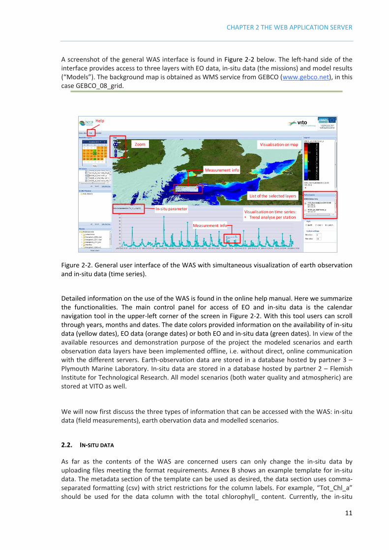
A screenshot of the general WAS interface is found in Figure 2-2 below. The left-hand side of the interface provides access to three layers with EO data, in-situ data (the missions) and model results (“Models”). The background map is obtained as WMS service from GEBCO (www.gebco.net), in this case GEBCO_08_grid.
Figure 2-2. General user interface of the WAS with simultaneous visualization of earth observation and in-situ data (time series).
Detailed information on the use of the WAS is found in the online help manual. Here we summarize the functionalities. The main control panel for access of EO and in-situ data is the calendar navigation tool in the upper-left corner of the screen in Figure 2-2. With this tool users can scroll through years, months and dates. The date colors provided information on the availability of in-situ data (yellow dates), EO data (orange dates) or both EO and in-situ data (green dates). In view of the available resources and demonstration purpose of the project the modeled scenarios and earth observation data layers have been implemented offline, i.e. without direct, online communication with the different servers. Earth-observation data are stored in a database hosted by partner 3 – Plymouth Marine Laboratory. In-situ data are stored in a database hosted by partner 2 – Flemish Institute for Technological Research. All model scenarios (both water quality and atmospheric) are stored at VITO as well.
We will now first discuss the three types of information that can be accessed with the WAS: in-situ data (field measurements), earth obervation data and modelled scenarios.
2.2. IN-SITU DATA
As far as the contents of the WAS are concerned users can only change the in-situ data by uploading files meeting the format requirements. Annex B shows an example template for in-situ data. The metadata section of the template can be used as desired, the data section uses comma-separated formatting (csv) with strict restrictions for the column labels. For example, “Tot_Chl_a” should be used for the data column with the total chlorophyll_ content. Currently, the in-situ
Help
Zoom
Visualisation on time series:• Trend analyse per station
Visualisation on map
List of the selected layers
Measurement info
In-situ parameter
Measurement info
CHAPTER 2 THE WEB APPLICATION SERVER
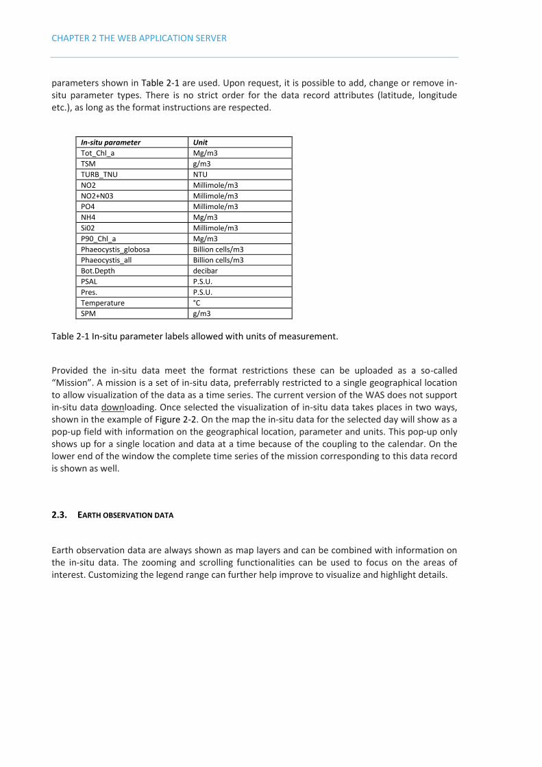
parameters shown in Table 2-1 are used. Upon request, it is possible to add, change or remove in-situ parameter types. There is no strict order for the data record attributes (latitude, longitude etc.), as long as the format instructions are respected.
In-situ parameter Unit
Tot_Chl_a Mg/m3
TSM g/m3
TURB_TNU NTU
NO2 Millimole/m3
NO2+N03 Millimole/m3
PO4 Millimole/m3
NH4 Mg/m3
Si02 Millimole/m3
P90_Chl_a Mg/m3
Phaeocystis_globosa Billion cells/m3
Phaeocystis_all Billion cells/m3
Bot.Depth decibar
PSAL P.S.U.
Pres. P.S.U.
Temperature °C
SPM g/m3
Table 2-1 In-situ parameter labels allowed with units of measurement.
Provided the in-situ data meet the format restrictions these can be uploaded as a so-called “Mission”. A mission is a set of in-situ data, preferrably restricted to a single geographical location to allow visualization of the data as a time series. The current version of the WAS does not support in-situ data downloading. Once selected the visualization of in-situ data takes places in two ways, shown in the example of Figure 2-2. On the map the in-situ data for the selected day will show as a pop-up field with information on the geographical location, parameter and units. This pop-up only shows up for a single location and data at a time because of the coupling to the calendar. On the lower end of the window the complete time series of the mission corresponding to this data record is shown as well.
2.3. EARTH OBSERVATION DATA
Earth observation data are always shown as map layers and can be combined with information on the in-situ data. The zooming and scrolling functionalities can be used to focus on the areas of interest. Customizing the legend range can further help improve to visualize and highlight details.

CHAPTER 2 THE WEB APPLICATION SERVER
13
2.4. MODEL SCENARIOS
We refer the ISECA Final Report D3.2 (De Kok et al., 2014b) For a more detailed description of the modelling of eutrophication. Two types of model scenarios are available in the WAS to demonstrate the potential use of model forecast: water quality scenarios for the chlorophyll-a content under different nitrogen load reduction strategies in the Scheldt basin (Vermaat et al., 2012; De Kok et al., 2014b) and atmospheric deposition scenarios. Different model simulations can be used to show the potential impact of different management strategies available to the EU member states. The model simulations are based on an empirical model for the dependency of the nutrient content and other parameters on the salinity, using sample data reported by the OSPAR workgroup in 2008 and a linear dependence on the nitrogen inflow from the main rivers. In addition, model simulations are available for the atmospheric deposition of eutrophication-related substances such as nitrogen oxides and ammonia from different sources.
2.4.1. WATER-BORNE INPUTS
Water-borne inputs of nutrients are an important cause of eutrophication. A simplified “proxy” model has been used for the WAS to demonstrate the potential of simulation modelling. The underlying model structure is shown below:
Figure 2-3 Steps in the simplified modelling process used to obtain the coastal and offshore chl-a values for different nitrogen loads for the Scheldt basin.
A more detailed description of the model architecture and functions used is found in Annex C. The model approximations include the following:
a. linear dependency between salinity and winter DIN concentration
Salinity data (sources: ICES)
Winter DIN (cf linear dependency )
Spring Chlorophyll-a(cf: OSPAR 2009)
2D interpolation
Scaling N balancemodel

CHAPTER 2 THE WEB APPLICATION SERVER
b. linear dependency winter DIN and spring chl-a/Phaeocystis cell count c. linear dependency slope of salinity-winter DIN relationship on N load contributing rivers d. influence rivers (for impact load reduction)salinity dependent and not overlapping
The spatial distribution in coastal waters has been obtained by two-dimensional interpolation of
salinity data provided by the ICES Oceanographic Database (ICES, 2012) and a “mixing diagram” for
the dependency between the winter DIN levels and practical salinity for the Belgian Coastal Waters
under pristine and actual conditions as reported by the Belgian OSPAR workgroup conditions
(OSPAR, 2008) during 2000-2005, and another linear relationship between the winter DIN and
spring chlorophyll-a content (OSPAR, 2008). The 2D interpolation is based on the inpainting
algorithm by John d’Errico (2006). The critical assessment (elevated) level is assumed to be 50 %
above the pristine level (OSPAR criterion). Finally, these scenarios are used for proportional
rescaling of the nitrogen concentrations in the coastal waters affected by the Scheldt effluents of
nutrients. Figure 2-4 shows the salinity gradient, used to translate estaurine values of the DIN level
into a spatially distributed salinity pattern.
Figure 2-4 Salinity distribution for the Southern North Sea and English Channel as obtained by 2D interpolation of ICES salinity data (ICES, 2012).
The results are intended for demonstration of the comparison of different management scenarios
in the WAS and have not been validated. A nitrogen balance model for the Scheldt river basin
(Vermaat et al., 2012; De Kok et al., 2014b) is used to estimate the yearly nitrogen load for each
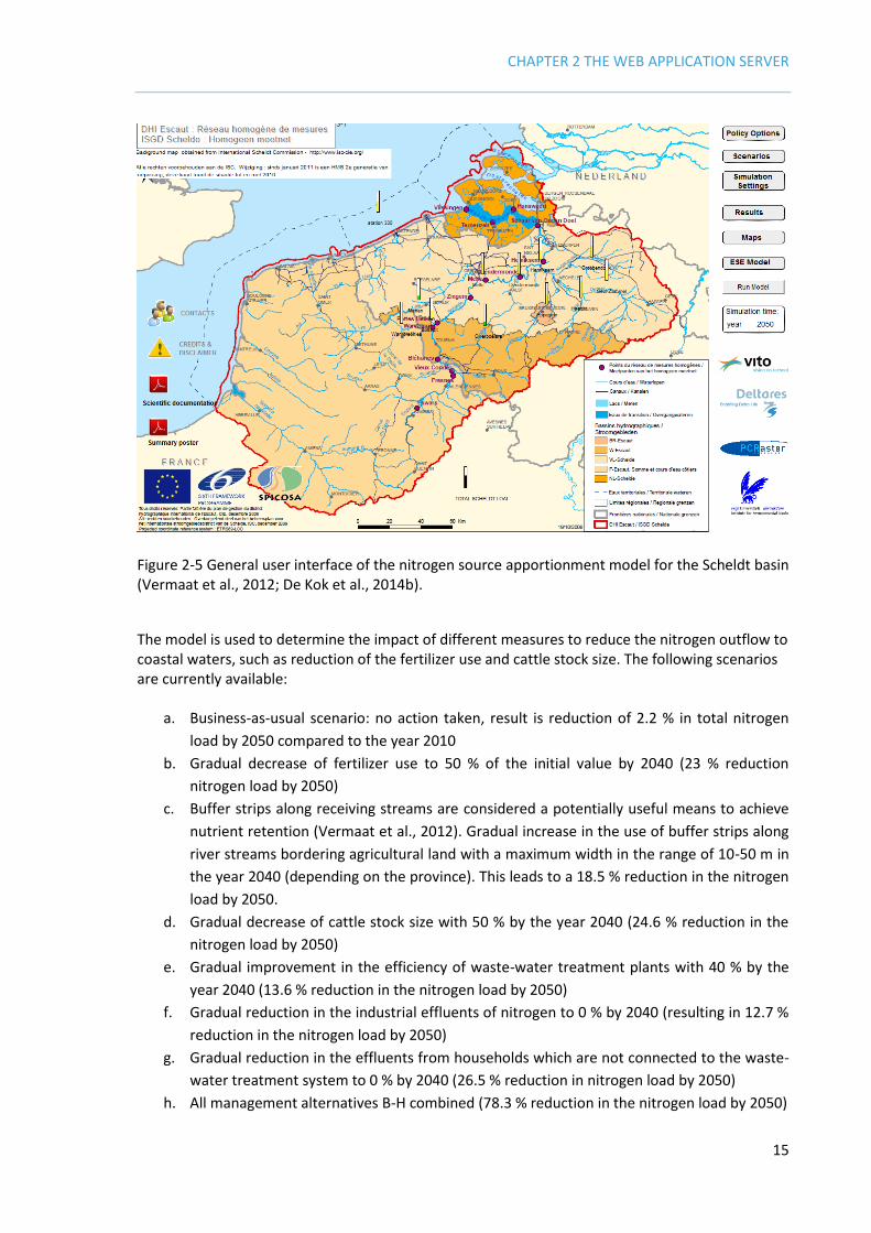
scenario (see Annex D for a summary of the nitrogen balance model). Figure 2-5 shows the general
interface of the model with quick access to scenarios, management options, and the model itself
with the maps used. Animated bar indicators change color during the simulation to indicate
changes in the nitrogen concentrations at specific measuring locations.
CHAPTER 2 THE WEB APPLICATION SERVER
15
Figure 2-5 General user interface of the nitrogen source apportionment model for the Scheldt basin (Vermaat et al., 2012; De Kok et al., 2014b).
The model is used to determine the impact of different measures to reduce the nitrogen outflow to coastal waters, such as reduction of the fertilizer use and cattle stock size. The following scenarios are currently available:
a. Business-as-usual scenario: no action taken, result is reduction of 2.2 % in total nitrogen
load by 2050 compared to the year 2010
b. Gradual decrease of fertilizer use to 50 % of the initial value by 2040 (23 % reduction
nitrogen load by 2050)
c. Buffer strips along receiving streams are considered a potentially useful means to achieve
nutrient retention (Vermaat et al., 2012). Gradual increase in the use of buffer strips along
river streams bordering agricultural land with a maximum width in the range of 10-50 m in
the year 2040 (depending on the province). This leads to a 18.5 % reduction in the nitrogen
load by 2050.
d. Gradual decrease of cattle stock size with 50 % by the year 2040 (24.6 % reduction in the
nitrogen load by 2050)
e. Gradual improvement in the efficiency of waste-water treatment plants with 40 % by the
year 2040 (13.6 % reduction in the nitrogen load by 2050)
f. Gradual reduction in the industrial effluents of nitrogen to 0 % by 2040 (resulting in 12.7 %
reduction in the nitrogen load by 2050)
g. Gradual reduction in the effluents from households which are not connected to the waste-
water treatment system to 0 % by 2040 (26.5 % reduction in nitrogen load by 2050)
h. All management alternatives B-H combined (78.3 % reduction in the nitrogen load by 2050)
CHAPTER 2 THE WEB APPLICATION SERVER
i. Business-as-usual with climate change scenario G – unchanged circulation pattern with 1
degree increase in temperature. KNMI 2006 Climate Change Scenarios see www.knmi.nl.
(results in 2 % reduction nitrogen load)
j. Business-as-usual with climate change scenario W+ – changed circulation pattern with 2
degree increase in temperature. KNMI 2006 Climate Change Scenarios see www.knmi.nl.
(results in 5.4 % reduction nitrogen load)
k. In addition two other scenarios are available: one for the pristine conditions (based on the mixing diagram reported in OSPAR(2008)), and one for the critical OSPAR threshold (50 % above the pristine level).
2.4.2. ATMOSPHERIC DEPOSITION
Atmospheric deposition scenarios are also available through the WAS. The atmospheric inputs of land- and sea-based emission sources such as industry and shipping are significant for eutrophication. For the Greater North Sea the average contribution of atmospheric inputs to the atmospheric depositions for the EMEP model over the years 1990-2004 was estimated to be 33 % (OSPAR, 2007). However, more detailed information on the emission and transport of substances such as NH3 and NOx is needed to understand the impact on marine eutrophication. This task is carried out by the Centre of Numerical Modelling and Process Analysis (CNMPA), of the University of Greenwich. High resolution (7x7 km) emission data were generated by VITO in October 2012 as part of an agreement to support this modelling activity. The annual emission data provided for the years 1990, 2000 and 2009 were obtained by downscaling officially reported national emissions with geospatial proxy data by means of a methodology which is also used by E-MAP (Maes et al., 2009). In addition, time profiles corresponding to the EMEP sectors were delivered to allow for temporal disaggregation at the level of months, days and hours. Three components are needed to achieve detailed modelling of the atmospheric inputs to eutrophication: (a) meteorological data, (b) emissions data and (c) modelling software for atmospheric transport and deposition. Freely downloadable meteorological data records from two different sources were considered: ECMWF Reanalysis data set ERA Interim 0.75 degree resolution (http://www.ecmwf.int) and NCEP (U.S.), Final Analysis, 1 degree resolution. The ECMWF data were chosen because of the slightly higher resolution, excellent compatibility with the LPD tracing software Flexpart (described below) and preference for European data. The records contain wind velocities, temperature, humidity, pressure, sunshine, precipitation and some other variables needed for the tracing model. The frequency of records is every 6 hours covering the period from 1979 until 2 months before real time.
The calculations were done with the open source, publicly available software FLEXPART (http://flexpart.eu) which is based on the Lagrangian Particle Dispersion method for tracing the movement of pollutants in the atmosphere and includes also algorithms for determining the rates of their deposition onto the ground or the sea surface. The validation of the model set up was done by comparing the concentrations of nitrogen oxides calculated by FLEXPART at a number of prescribed receptor points on the ground in Kent, UK with the corresponding measurements from a publicly available dataset (http://www.kentair.org.uk/data/data-selector). On the WAS webpages, the results of the computer modelling are presented for the transport by air of nitrogen oxides and ammonia from their sources to the coastal waters in the 2Seas region. The examples provided are for emissions in 2000 and 2009 and historical weather data for 2009 and 2011. All four combinations between these emission and simulation years are included, so that comparisons can be made and the effect of both the emissions and the weather can be demonstrated. The

CHAPTER 2 THE WEB APPLICATION SERVER
17
atmospheric inputs of nitrogen nutrients are presented as deposition maps for the first 4 months of the studied years and for complete years. The period of the first 4 months was chosen because in the Southern North Sea, harmful algal blooms due to eutrophication usually happen in April. Total quantities of nitrogen oxides and ammonia are presented as well as specific maps of deposition resulting from road and other transport. The main conclusions are:
• Ammonia is responsible for the largest share of nitrogen deposits from the atmosphere; being more soluble, ammonia tends to get deposited not far from the source.
• Nitrogen oxides emissions are more likely to leave the region and be deposited elsewhere. (Far-away emissions which may be carried by the wind and be deposited in the 2Seas region are not part of these simulations.)
• Heavy nutrient load onto the coastal waters of Belgium and the Netherlands is observed in all model scenarios.
2.5. USER FEEDBACK AND RECOMMENDATIONS
As explained the current version of the WAS is a demonstration instrument, mainly designed for the visualization of existing data. Downloading of data is not yet possible. In-situ data can be uploaded as files, and will become accessible through the calendar tool. Earth observation data layers and model simulations cannot be uploaded directly by users of the WAS.
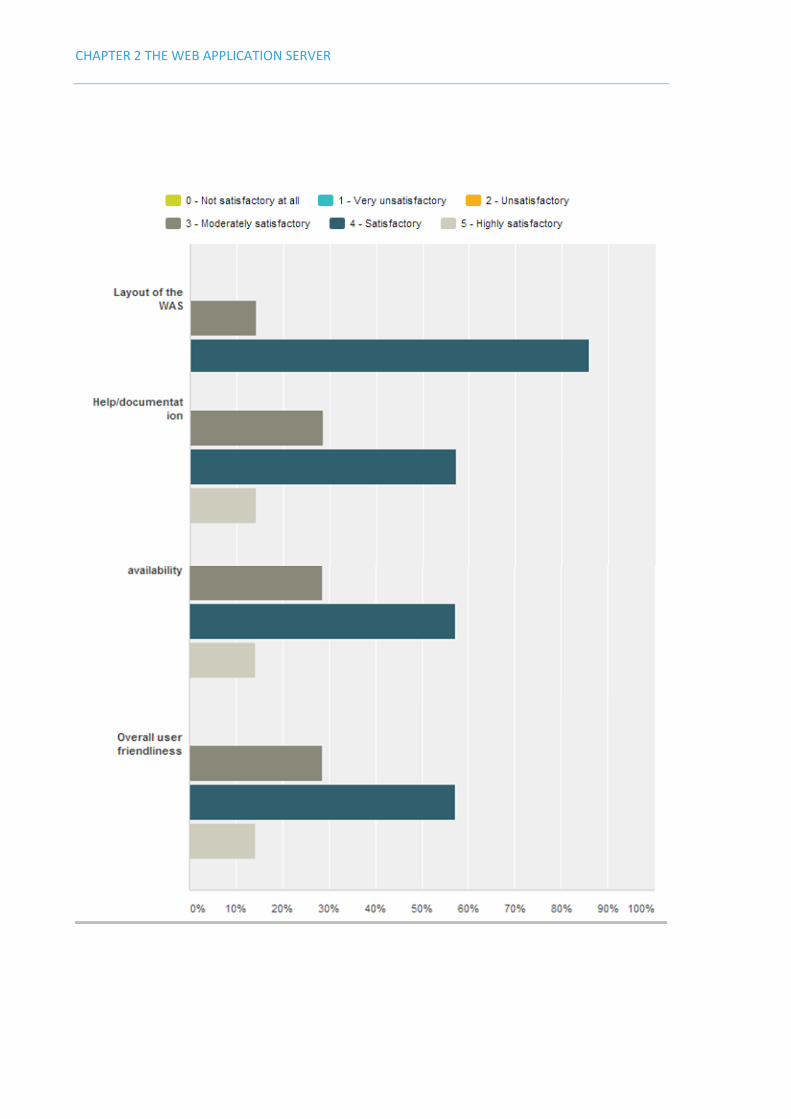
A first user confrontation of the WAS occurred during an interactive workshop which was held during the ISECA final meeting in Boulogne-sur-Mèr (F) on July 1, 2014. The workshop participants were given a number of exercises to familiarize themselves with the WAS in a 2-hour session. As expected this also proved to be a good opportunity to obtain feedback on the functionalities and many useful suggestions for adaptation or improvement were given. The participants were of a mixed background (scientists, regional water managers, farmers and industry).
The main conclusions and recommendations were the following:
The design of the Web Application Server is intuitive and the WAS is easy to use in general with the calendar navigation to query data
Although the WAS could be very useful, the indicators shown are too scientific for non-experts, who would like to be given more basic information such as a problem or no problem, or an algal bloom risk map
Depending on the screen resolution there were technical with some subwindows which could be solved with some effort. The WAS does not work on iPADs.
The documentation should be expanded, and needs to be clearer sometimes.
In principle there are no limitations to the uploading of in-situ data, quality control is an issue. For the time being this is solved with a Data Policy Statement on the web site. This can be considered less of a problem when the uploading facility is (temporarily) disabled.
Who maintains the WAS? It has been decided that VITO carries out limited maintenance on the WAS for a number of years, VLIZ will do the same with the general project web site.
An online survey was held to evaluate the WAS. The first results (beginning July, 2014) are shown below.
CHAPTER 2 THE WEB APPLICATION SERVER
CHAPTER 3 WEB APPLICATION SERVER FUNCTIONALITY
19
CHAPTER 3 WEB APPLICATION SERVER FUNCTIONALITY
3.1. INTRODUCTION
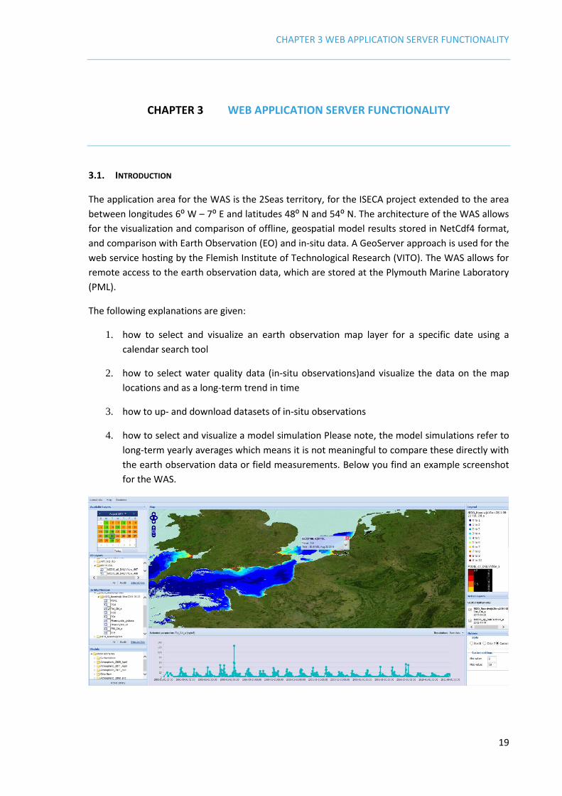
The application area for the WAS is the 2Seas territory, for the ISECA project extended to the area
between longitudes 6⁰ W – 7⁰ E and latitudes 48⁰ N and 54⁰ N. The architecture of the WAS allows
for the visualization and comparison of offline, geospatial model results stored in NetCdf4 format,
and comparison with Earth Observation (EO) and in-situ data. A GeoServer approach is used for the
web service hosting by the Flemish Institute of Technological Research (VITO). The WAS allows for
remote access to the earth observation data, which are stored at the Plymouth Marine Laboratory
(PML).
The following explanations are given:
1. how to select and visualize an earth observation map layer for a specific date using a
calendar search tool
2. how to select water quality data (in-situ observations)and visualize the data on the map
locations and as a long-term trend in time
3. how to up- and download datasets of in-situ observations
4. how to select and visualize a model simulation Please note, the model simulations refer to
long-term yearly averages which means it is not meaningful to compare these directly with
the earth observation data or field measurements. Below you find an example screenshot
for the WAS.
CHAPTER 3 WEB APPLICATION SERVER FUNCTIONALITY
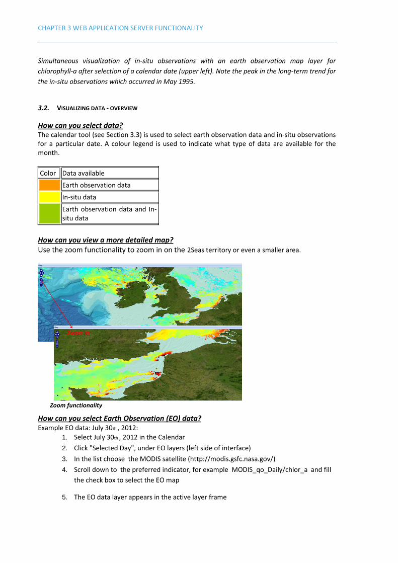
Simultaneous visualization of in-situ observations with an earth observation map layer for
chlorophyll-a after selection of a calendar date (upper left). Note the peak in the long-term trend for
the in-situ observations which occurred in May 1995.
3.2. VISUALIZING DATA - OVERVIEW
How can you select data? The calendar tool (see Section 3.3) is used to select earth observation data and in-situ observations for a particular date. A colour legend is used to indicate what type of data are available for the month.
Color Data available
Earth observation data
In-situ data
Earth observation data and In-situ data
How can you view a more detailed map? Use the zoom functionality to zoom in on the 2Seas territory or even a smaller area.
Zoom functionality
How can you select Earth Observation (EO) data? Example EO data: July 30th , 2012:
1. Select July 30th , 2012 in the Calendar
2. Click "Selected Day", under EO layers (left side of interface)
3. In the list choose the MODIS satellite (http://modis.gsfc.nasa.gov/)
4. Scroll down to the preferred indicator, for example MODIS_qo_Daily/chlor_a and fill
the check box to select the EO map
5. The EO data layer appears in the active layer frame
CHAPTER 3 WEB APPLICATION SERVER FUNCTIONALITY
21
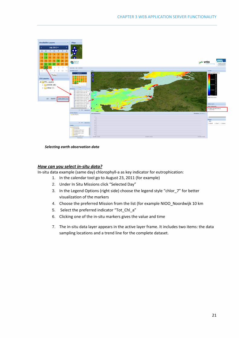
Selecting earth observation data
How can you select in-situ data? In-situ data example (same day) chlorophyll-a as key indicator for eutrophication:
1. In the calendar tool go to August 23, 2011 (for example)
2. Under In Situ Missions click “Selected Day”
3. In the Legend Options (right side) choose the legend style “chlor_7” for better
visualization of the markers
4. Choose the preferred Mission from the list (for example NIOO_Noordwijk 10 km
5. Select the preferred indicator “Tot_Chl_a”
6. Clicking one of the in-situ markers gives the value and time
7. The in-situ data layer appears in the active layer frame. It includes two items: the data
sampling locations and a trend line for the complete dataset.

CHAPTER 3 WEB APPLICATION SERVER FUNCTIONALITY
Selecting in-situ data
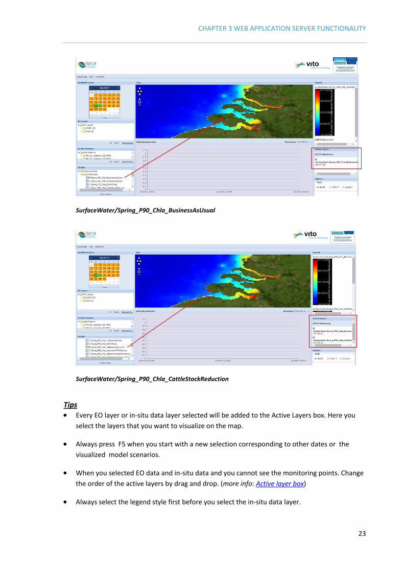
How can you visualize model scenarios? Model scenarios or simulations are not related to particular date or year but based on spring-average for period 2005-2012 using OSPAR assumptions. More details are given in Section 6 – Model Scenarios. The technical steps are:
1. The recommendation is to undo the earlier selections under “Active Layers” on the
right-hand side first or press the function key F5 (refresh)
2. Zoom in on the Belgian coastal waters for a better view
3. Go to the Models menu (lower left)
4. Under “Model data” select the preferred model theme, for example 'SurfaceWater'
and then the preferred scenario, for example “Spring_P90_Chla_BusinessAsUsual - this
is a scenario without additional management measures to reduce the five-year
average nutrient load from the Scheldt basin
5. Leave the image and select (for example) the scenario
“ScenariosBCZ/Spring_Chla_CattleStockReduction” to see the difference in water
quality
6. Both model scenarios layers appear in the active layer frame and you can check or
uncheck the layers to see the difference in water quality
CHAPTER 3 WEB APPLICATION SERVER FUNCTIONALITY
23
SurfaceWater/Spring_P90_Chla_BusinessAsUsual
SurfaceWater/Spring_P90_Chla_CattleStockReduction
Tips
Every EO layer or in-situ data layer selected will be added to the Active Layers box. Here you
select the layers that you want to visualize on the map.
Always press F5 when you start with a new selection corresponding to other dates or the
visualized model scenarios.
When you selected EO data and in-situ data and you cannot see the monitoring points. Change
the order of the active layers by drag and drop. (more info: Active layer box)
Always select the legend style first before you select the in-situ data layer.
CHAPTER 3 WEB APPLICATION SERVER FUNCTIONALITY
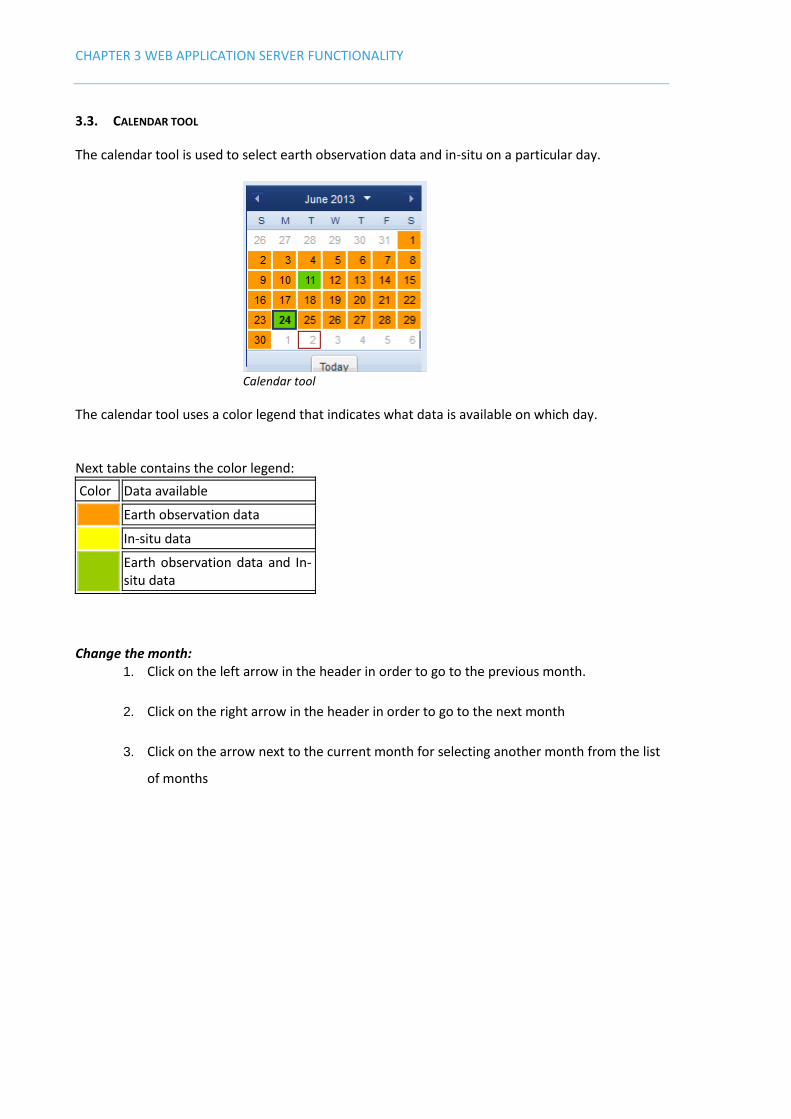
3.3. CALENDAR TOOL
The calendar tool is used to select earth observation data and in-situ on a particular day.
Calendar tool
The calendar tool uses a color legend that indicates what data is available on which day. Next table contains the color legend:
Color Data available
Earth observation data
In-situ data
Earth observation data and In-situ data
Change the month: 1. Click on the left arrow in the header in order to go to the previous month.
2. Click on the right arrow in the header in order to go to the next month
3. Click on the arrow next to the current month for selecting another month from the list
of months

CHAPTER 3 WEB APPLICATION SERVER FUNCTIONALITY
25
Change from month
Select a particular day: o Click on a particular day in the selected month
Select current day: o Click on the button 'Today' and the calendar tool selects the current day. This is an in-
built option. Usually the system is not yet updated for the actual date.

CHAPTER 3 WEB APPLICATION SERVER FUNCTIONALITY
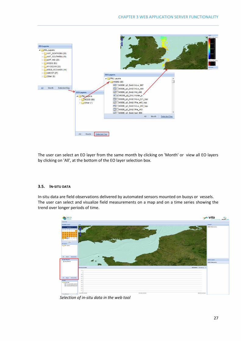
3.4. EARTH OBSERVATION DATA
The earth observation data are stored at the Plymouth Marine Laboratory (PML). The user can select and visualize an earth observation data layer for specific dates using the calendar search tool
Selection of EO layers starts with the calendar tool
Select an EO layer on a selected day:
1. Select a particular day in the calendar tool
2. Click on 'Selected day' in the EO layer selection box and the corresponding EO layers
are displayed, grouped in folders.
3. Open a folder
4. Select a particular EO layer and this map layer will be visualized on the screen
CHAPTER 3 WEB APPLICATION SERVER FUNCTIONALITY
27
The user can select an EO layer from the same month by clicking on 'Month' or view all EO layers by clicking on 'All', at the bottom of the EO layer selection box.
3.5. IN-SITU DATA
In-situ data are field observations delivered by automated sensors mounted on buoys or vessels. The user can select and visualize field measurements on a map and on a time series showing the trend over longer periods of time.
Selection of in-situ data in the web tool

CHAPTER 3 WEB APPLICATION SERVER FUNCTIONALITY
Related functionalities are:
o Select in-situ data
o View in-situ data
o Colored measurement points
o Upload in-situ data
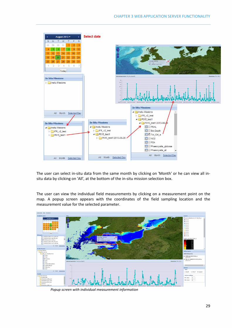
Select in-situ data on a selected day:
1. Select a particular day in the calendar tool
2. Click on 'Selected day' in the In-situ mission selection box and the corresponding in-situ
data are displayed, grouped in folders.
3. Open a folder
4. Select a particular in-situ mission. A mission is a dataset which has been uploaded by
other users of the WAS.
5. Select a parameter, e.g. the total chlorophyll-a value (“Tot_Chl_a”). The indicator for
the selected mission will be visualized on the map, and the field measurements on the
time trend line at the bottom of your screen.
CHAPTER 3 WEB APPLICATION SERVER FUNCTIONALITY
29
The user can select in-situ data from the same month by clicking on 'Month' or he can view all in-situ data by clicking on 'All', at the bottom of the in-situ mission selection box.
The user can view the individual field measurements by clicking on a measurement point on the map. A popup screen appears with the coordinates of the field sampling location and the measurement value for the selected parameter.
Popup screen with individual measurement information

CHAPTER 3 WEB APPLICATION SERVER FUNCTIONALITY
The popup screen gives the coordinates, the measurement value, the measurement time and the source.
Detail of the pop-up information provided for the sampling location.
The web tool provides the possibility to colour the measurement points on the map so that locations with high concentrations, hot spots, are easy to recognize. Coloring of the measurement points:
1. Select a specific legend style
2. Select the in-situ data and the measurement points are automatically colored
corresponding the measurement values.
See Section 9 for more details on the use of the Legend Tool.
3.6. UPLOADING IN-SITU DATA
The user can also upload datasets of in-situ observations (“missions”) into the WAS. The datasets
are to be in comma-separated files or CSV format.
Preparing the upload file.
Before starting the upload of in-situ data, this checklist should be followed:
1. Only registered in-situ parameters 1are allowed. (see in-situ parameters)
2. Provide one upload file per fixed measurement location (station).
This is important for the visualization of the trend analysis per fixed station.
3. The data must be sorted in chronologic al order
4. The upload file must be in accordance with the template file provided.
1 Registered in-situ parameters are parameters defined in the WAS application.

CHAPTER 3 WEB APPLICATION SERVER FUNCTIONALITY
31
The upload file must contain at least the columns Cruise, Station, Type, Time, Lon, Lat and Source. The in-situ parameters must be in accordance with the registered in-situ parameters.
Upload in-situ data.
1. Click on 'Upload data' and next screen appears:
2. Enter a mission name, for example “Belgian_Coast_Nov_2013)
3. Enter a meaningful operator name, for example “DrMatthews_VITO”
4. Select your data file by using the 'Browse' button
5. Click on 'Upload'
6. The following error messages may appear
Errors
Error Explanation
Err_missing_metadataend The word 'metadata_labels_end' is missing in the file. Please check the upload file.
Decreasing line date at line [line number]
The data is not sorted in descending order by time. Please check the upload file.
Source [Source value] not length 3 in line [line number]
The source can contain max. 3 characters. Please the upload file.
More items in line [line number] than in header
The header is missing one or more columns compared with the data. Please check the upload file.
Wrong size createtimestamp for [timestamp] line [line number]
The time has a wrong format in line [line number]. Please check the upload file.
CHAPTER 3 WEB APPLICATION SERVER FUNCTIONALITY
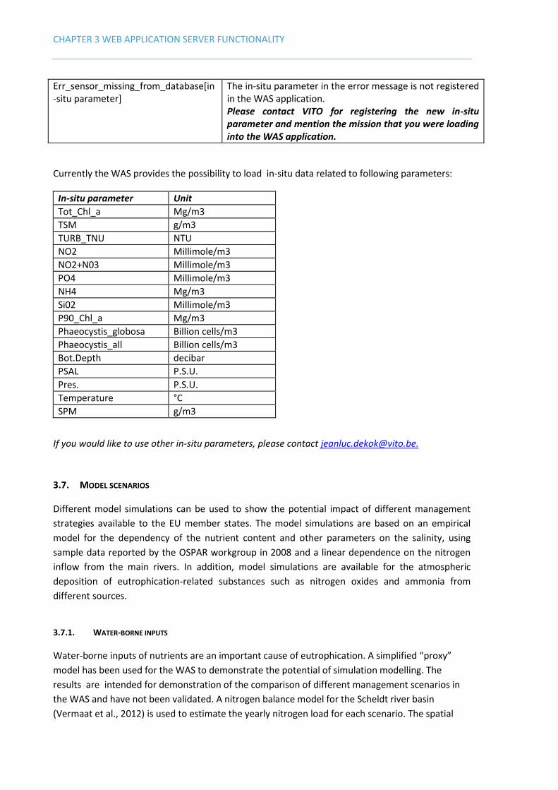
Err_sensor_missing_from_database[in-situ parameter]
The in-situ parameter in the error message is not registered in the WAS application. Please contact VITO for registering the new in-situ parameter and mention the mission that you were loading into the WAS application.
Currently the WAS provides the possibility to load in-situ data related to following parameters:
In-situ parameter Unit
Tot_Chl_a Mg/m3
TSM g/m3
TURB_TNU NTU
NO2 Millimole/m3
NO2+N03 Millimole/m3
PO4 Millimole/m3
NH4 Mg/m3
Si02 Millimole/m3
P90_Chl_a Mg/m3
Phaeocystis_globosa Billion cells/m3
Phaeocystis_all Billion cells/m3
Bot.Depth decibar
PSAL P.S.U.
Pres. P.S.U.
Temperature °C
SPM g/m3
If you would like to use other in-situ parameters, please contact [email protected].
3.7. MODEL SCENARIOS
Different model simulations can be used to show the potential impact of different management
strategies available to the EU member states. The model simulations are based on an empirical
model for the dependency of the nutrient content and other parameters on the salinity, using
sample data reported by the OSPAR workgroup in 2008 and a linear dependence on the nitrogen
inflow from the main rivers. In addition, model simulations are available for the atmospheric
deposition of eutrophication-related substances such as nitrogen oxides and ammonia from
different sources.
3.7.1. WATER-BORNE INPUTS
Water-borne inputs of nutrients are an important cause of eutrophication. A simplified “proxy”
model has been used for the WAS to demonstrate the potential of simulation modelling. The
results are intended for demonstration of the comparison of different management scenarios in
the WAS and have not been validated. A nitrogen balance model for the Scheldt river basin
(Vermaat et al., 2012) is used to estimate the yearly nitrogen load for each scenario. The spatial

CHAPTER 3 WEB APPLICATION SERVER FUNCTIONALITY
33
distribution in coastal waters has been obtained by two-dimensional interpolation of salinity data
provided by the ICES Oceanographic Database (ICES, 2012) and a “mixing diagram” for the
dependency between the winter DIN levels and practical salinity for the Belgian Coastal Waters
under pristine and actual conditions as reported by the Belgian OSPAR workgroup conditions
(OSPAR, 2008) during 2000-2005, and another linear relationship between the winter DIN and
spring chlorophyll-a content (OSPAR, 2008). The 2D interpolation is based on the inpainting
algorithm by John d’Errico (2006). The critical assessment (elevated) level is assumed to be 50 %
above the pristine level (OSPAR criterion). Finally, these scenarios are used for proportional
rescaling of the nitrogen concentrations in the coastal waters affected by the Scheldt effluents of
nutrients. The model is used to determine the impact of different measures to reduce the nitrogen
outflow to coastal waters, such as reduction of the fertilizer use and cattle stock size. The following
scenarios are currently available:
1. Business-as-usual scenario: no action taken, result is reduction of 2.2 % in total nitrogen
load by 2050 compared to the year 2010
2. Gradual decrease of fertilizer use to 50 % of the initial value by 2040 (23 % reduction
nitrogen load by 2050)
3. Buffer strips along receiving streams are considered a potentially useful means to achieve
nutrient retention (Vermaat et al., 2012). Gradual increase in the use of buffer strips along
river streams bordering agricultural land with a maximum width in the range of 10-50 m in
the year 2040 (depending on the province). This leads to a 18.5 % reduction in the nitrogen
load by 2050.
4. Gradual decrease of cattle stock size with 50 % by the year 2040 (24.6 % reduction in the
nitrogen load by 2050)
5. Gradual improvement in the efficiency of waste-water treatment plants with 40 % by the
year 2040 (13.6 % reduction in the nitrogen load by 2050)
6. Gradual reduction in the industrial effluents of nitrogen to 0 % by 2040 (resulting in 12.7 %
reduction in the nitrogen load by 2050)
7. Gradual reduction in the effluents from households which are not connected to the waste-
water treatment system to 0 % by 2040 (26.5 % reduction in nitrogen load by 2050)
8. All management alternatives B-H combined (78.3 % reduction in the nitrogen load by 2050)
9. Business-as-usual with climate change scenario G – unchanged circulation pattern with 1
degree increase in temperature. KNMI 2006 Climate Change Scenarios see www.knmi.nl.
(results in 2 % reduction nitrogen load)
10. Business-as-usual with climate change scenario W+ – changed circulation pattern with 2
degree increase in temperature. KNMI 2006 Climate Change Scenarios see www.knmi.nl.
(results in 5.4 % reduction nitrogen load)
It is not possible for general users to add model scenarios. This should be done by the WAS host institute (i.e. VITO) and involves three steps:
1. Logon in to the samba server by entering exactly the following line in the DOS box (note
the spaces!):
“net use \\samba.rma.vito.local /user:username” (fill in your user name in username)

CHAPTER 3 WEB APPLICATION SERVER FUNCTIONALITY
This will prompt for a password (usually root-specific and different from the network password). 2. In Win Explorer: Map network drive and enter the following path exactly:
\\samba.rma.vito.local\iseca\ncWMS-data This will open the folder with the model scenario (NetCDF) files. 3. The administrative tasks related to the management of the model scenarios can be fulfilled
through the following URL: http://isecancwms.rma.vito.local:8080/ncWMS/ . Clicking on the option “Admin Interface” will open a login screen. After login the following screen will appear for administrative tasks:
Figure 3-1. Administrative interface for definition of the model scenarios to be shown.
3.7.2. ATMOSPHERIC DEPOSITION
Atmospheric deposition scenarios are also available through the WAS. The atmospheric inputs of land- and sea-based emission sources such as industry and shipping are significant for eutrophication. For the Greater North Sea the average contribution of atmospheric inputs to the atmospheric depositions for the EMEP model over the years 1990-2004 was estimated to be 33 % (OSPAR, 2007). However, more detailed information on the emission and transport of substances such as NH3 and NOx is needed to understand the impact on marine eutrophication. This task is carried out by the Centre of Numerical Modelling and Process Analysis (CNMPA), of the University of Greenwich. High resolution (7x7 km) emission data were generated by VITO in October 2012 as part of an agreement to support this modelling activity. The annual emission data provided for the years 1990, 2000 and 2009 were obtained by downscaling officially reported national emissions with geospatial proxy data by means of a methodology which is also used by E-MAP (Maes et al., 2009). In addition, time profiles corresponding to the EMEP sectors were delivered to allow for temporal disaggregation at the level of months, days and hours. Three components are needed to achieve detailed modelling of the atmospheric inputs to eutrophication: (a) meteorological data, (b) emissions data and (c) modelling software for atmospheric transport and deposition. Freely

CHAPTER 3 WEB APPLICATION SERVER FUNCTIONALITY
35
downloadable meteorological data records from two different sources were considered: ECMWF Reanalysis data set ERA Interim 0.75 degree resolution (http://www.ecmwf.int) and NCEP (U.S.), Final Analysis, 1 degree resolution. The ECMWF data were chosen because of the slightly higher resolution, excellent compatibility with the LPD tracing software Flexpart (described below) and preference for European data. The records contain wind velocities, temperature, humidity, pressure, sunshine, precipitation and some other variables needed for the tracing model. The frequency of records is every 6 hours covering the period from 1979 until 2 months before real time.
The calculations were done with the open source, publicly available software FLEXPART (http://flexpart.eu) which is based on the Lagrangian Particle Dispersion method for tracing the movement of pollutants in the atmosphere and includes also algorithms for determining the rates of their deposition onto the ground or the sea surface. The validation of the model set up was done by comparing the concentrations of nitrogen oxides calculated by FLEXPART at a number of prescribed receptor points on the ground in Kent, UK with the corresponding measurements from a publicly available dataset (http://www.kentair.org.uk/data/data-selector). On the WAS webpages, the results of the computer modelling are presented for the transport by air of nitrogen oxides and ammonia from their sources to the coastal waters in the 2Seas region. The examples provided are for emissions in 2000 and 2009 and historical weather data for 2009 and 2011. All four combinations between these emission and simulation years are included, so that comparisons can be made and the effect of both the emissions and the weather can be demonstrated. The atmospheric inputs of nitrogen nutrients are presented as deposition maps for the first 4 months of the studied years and for complete years. The period of the first 4 months was chosen because in the Southern North Sea, harmful algal blooms due to eutrophication usually happen in April. Total quantities of nitrogen oxides and ammonia are presented as well as specific maps of deposition resulting from road and other transport. The main conclusions are:
• Ammonia is responsible for the largest share of nitrogen deposits from the atmosphere; being more soluble, ammonia tends to get deposited not far from the source.
• Nitrogen oxides emissions are more likely to leave the region and be deposited elsewhere. (Far-away emissions which may be carried by the wind and be deposited in the 2Seas region are not part of these simulations.)
• Heavy nutrient load onto the coastal waters of Belgium and the Netherlands is observed in all model scenarios.
CHAPTER 3 WEB APPLICATION SERVER FUNCTIONALITY
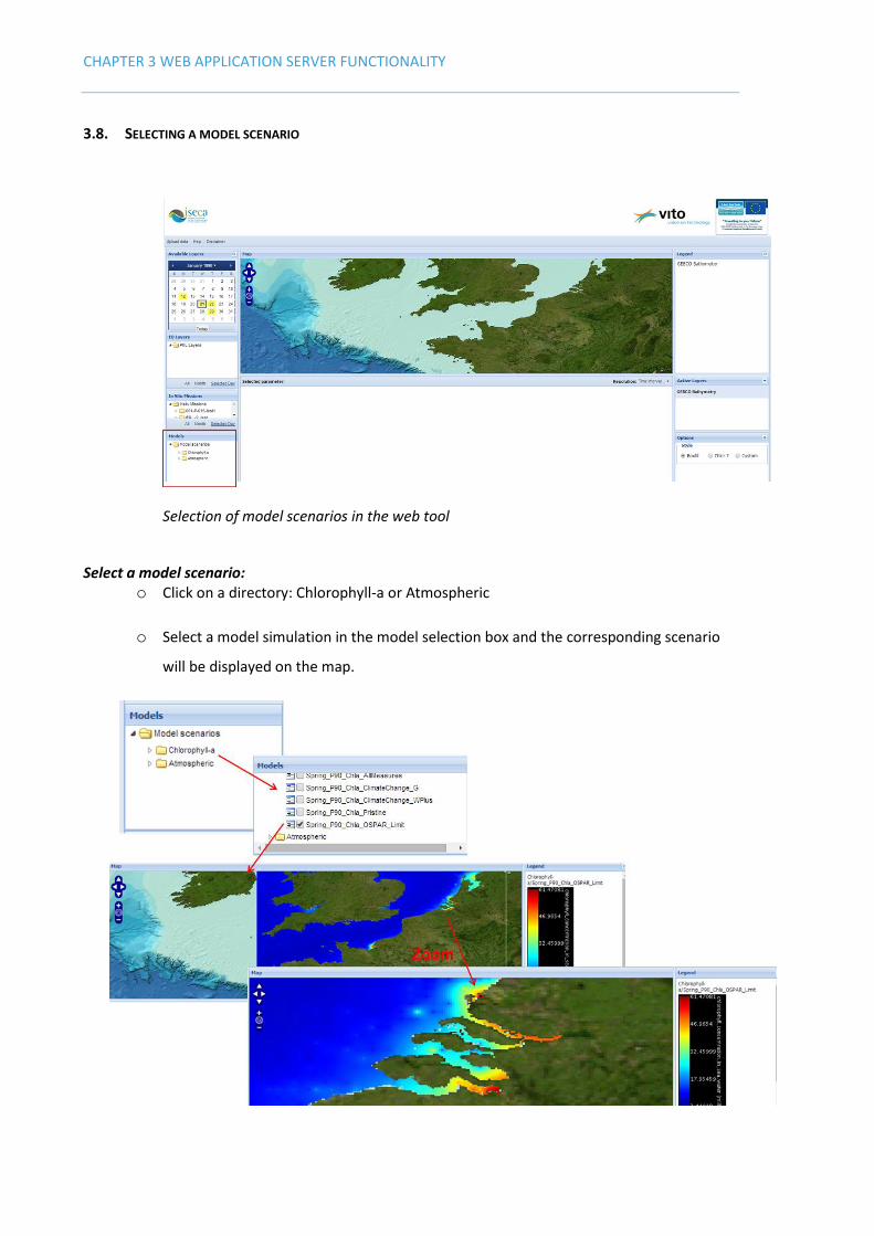
3.8. SELECTING A MODEL SCENARIO
Selection of model scenarios in the web tool
Select a model scenario: o Click on a directory: Chlorophyll-a or Atmospheric
o Select a model simulation in the model selection box and the corresponding scenario
will be displayed on the map.

CHAPTER 3 WEB APPLICATION SERVER FUNCTIONALITY
37
3.9. MODEL LIBRARY
The effort to design, implement and validate integrated models of environmental systems is often considerable. Following the practice in engineering and manufacturing, a component-based approach could facilitate the development and exchange of model constructs between researchers (De Kok et al., 2010; De Kok et al., 2014a; De Kok et al., 2014b). The idea of a generic model libraries to use reusable components for integrated systems modelling (Hopkins et al., 2011) was one of the deliverables of the EU-FP6 research project SPICOSA (http://www.spicosa.eu). This facilitates the construction of models, exchange of model constructs between research teams, and the maintenance of models. The project used ExtendSim (www.extendsim.com ) as common simulation modelling framework. The majority of the 18 SPICOSA case studies concerned coastal eutrophication and shell species culture, making these very relevant for the ISECA project. In ISECA the case study model for nitrogen transport in the Westerscheldt Estuary (Vermaat et al., 2012) was further developed and used to estimate nitrogen concentrations in the Belgian coastal waters and use these for the “SurfaceWater” model scenarios in the WAS. . A number of case study models and demo version of ExtendSim can be downloaded and installed through the hyperlink provided here. The SPICOSA model library and some example models are accessible through the “Model Library” button on the lower left of the WAS interface.
3.10. USE OF THE ACTIVE LAYER BOX
The active layer box allows the user to change the sequence of the layers with drag and drop, and
the user can select or deselect a particular layer. The layers appears automatically in the active
layer box when the user selects an EO layer, in-situ data or a model scenario. The top layer of the
map corresponds with the bottom map in the active layer box.
Deselect the top layer gives:

CHAPTER 3 WEB APPLICATION SERVER FUNCTIONALITY
Changing the sequence of the layers gives:
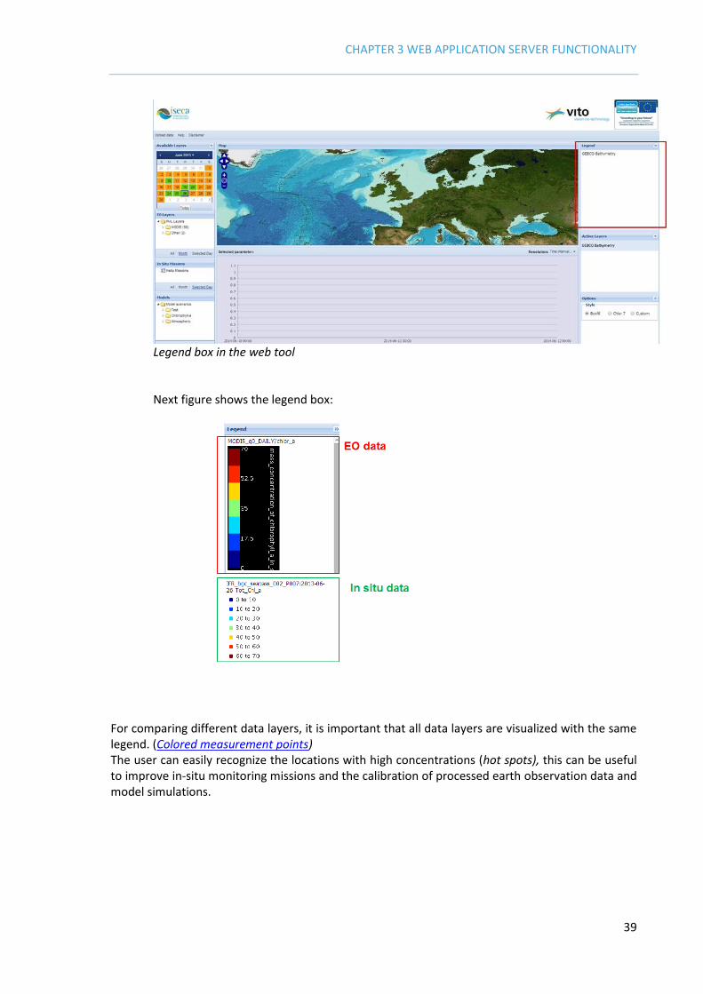
3.11. SETTING THE COLOR LEGEND
The legend box displays the legends of the different selected active layers (Active layer box).
CHAPTER 3 WEB APPLICATION SERVER FUNCTIONALITY
39
Legend box in the web tool Next figure shows the legend box:
For comparing different data layers, it is important that all data layers are visualized with the same legend. (Colored measurement points) The user can easily recognize the locations with high concentrations (hot spots), this can be useful to improve in-situ monitoring missions and the calibration of processed earth observation data and model simulations.

CHAPTER 3 WEB APPLICATION SERVER FUNCTIONALITY
Integration of in-situ data with earth observation data with the same legend
Remark: It is important that all layers (EO data layer, in-situ data layer, model data layer) uses the same legend for the same parameter.
The legend Style box contains the different styles for coloring the in-situ measurement points. (see Colored measurement points)
Legend styles
Three options for the legend styles are provided:
1. Boxfill
Boxfill is by default selected and is used to visualize the in-situ measurement points.
2. Chlor 7

CHAPTER 3 WEB APPLICATION SERVER FUNCTIONALITY
41
Select Chlor 7 when you want to visualize the measurements related to the parameter Tot_Chlor_a
3. Custom
Select Custom when you want to visualize the measurements related to other parameters. Here you define the min. and the max. value for generating the legend style.
How to use?
1. Select always first the legend style before you select the in-situ data layer or the EO
layer, for instance select the legend style 'Custom' and an EO layer
Legend style 'Custom' is selected before the selection of the EO layer
2. Change the max. value from 70 to 10
3. Reselect the EO layer in the EO layers box
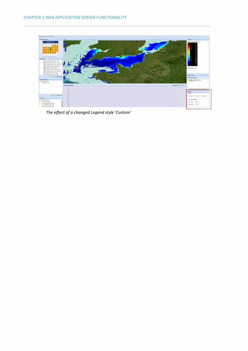
CHAPTER 3 WEB APPLICATION SERVER FUNCTIONALITY
The effect of a changed Legend style 'Custom'

CHAPTER 3 WEB APPLICATION SERVER FUNCTIONALITY
43
3.12. TREND ANALYSIS OF IN-SITU DATA TIME SERIES
Trends are visualized as a time series, when possible. The time series displays the measurement values of the selected parameter in a mission for the whole period. The figure below shows an example of a trend for total chlorophyll-a value for the period of 1990 until 2011. The user can select a point on the graph to view the individual measurement in the time series.
CHAPTER 3 WEB APPLICATION SERVER FUNCTIONALITY
BIBLIOGRAPHY
De Kok, J.L., Engelen, G. and Maes, J., 2010. Towards Model Component Reuse for the Design of Simulation Models – A Case Study for ICZM, Proceedings 2010 International Congress on Environmental Modelling and Software Modelling for Environment’s Sake, Fifth Biennial Meeting, Ottawa, Canada. Swayne DA, Yang W, Voinov AA, Rizzoli A and Filatova T. (Eds.). Volume 2, page 1208-1215. De Kok JL, Engelen G and Maes J., 2014a. Reusability of model components for environmental simulation – Case studies for integrated coastal zone management. Environmental Modelling & Software. Resubmitted. De Kok JL, Poelmans L, Van Esch E, Uljee I, Engelen G, Veldeman N, 2014b. Eutrophication problems, causes and potential solutions, and exchange of reusable model building components for the integrated simulation of coastal eutrophication. ISECA Final Report D3.2. John d'Errico (2006). http://www.mathworks.com/matlabcentral/fileexchange/4551 Hopkins, T.S., Bailly, D. and Stǿttrup, J.G., 2011. A Systems Approach Framework for Coastal Zones. Special Issue - Ecology and Society 16(4): 25. ICES, 2012. International Council for the Exploration of the Sea Oceanographic Database. 2012. ICES, Copenhagen. www.ices.dk Maes J, Vliegen J, Van de Vel K, Janssen S, Deutsch F, De Ridder K. Spatial surrogates for the disaggregation of CORINAIR emission inventories, Atmospheric Environment, 2009, 43, 1246-1254. OSPAR, 2007. Bartnicki J and Fagerli H. Atmospheric nitrogen in the OSPAR convention area in the period 1990-2004. EMES/MCS-W Technical report 4/2006. OSPAR Eutrophication Series, publication 344/2007. OSPAR Commission, 2007. www.ospar.org OSPAR, 2008. Report on the second application of the OSPAR Comprehensive procedure to the Belgian Marine Waters. Report by Belgium. Federal Public Service Health, Food Chain Safety and Environment, 70 pages. 2008. www.ospar.org Vermaat, J.E., Broekx, S., Van Eck, B., Engelen, G., Hellmann, F., De Kok, J.L., Van der Kwast, H., Maes, J., Salomons, W. and Van Deursen, W., 2012. Nitrogen source apportionment for the catchment, estuary and adjacent coastal waters of the Scheldt, Special Issue - A Systems Approach for Sustainable Development in Coastal Zones, Ecology and Society 17(2): 30.
CHAPTER 3 WEB APPLICATION SERVER FUNCTIONALITY
45
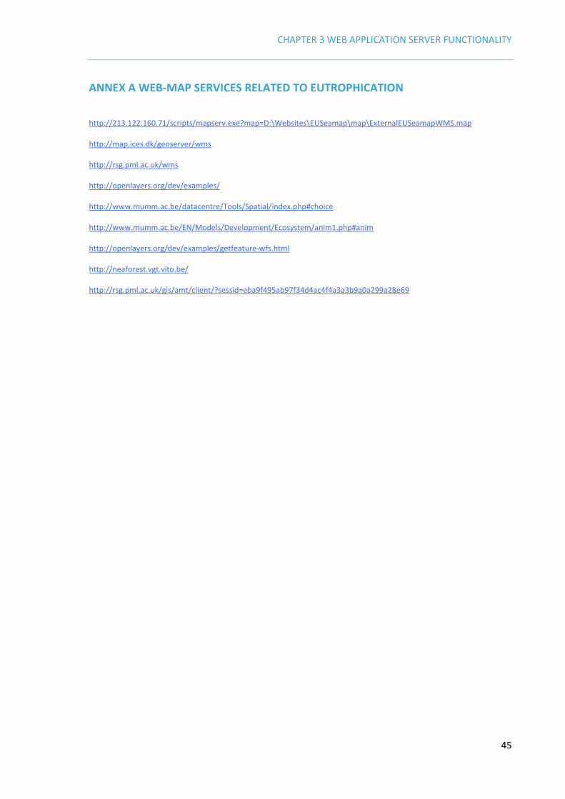
ANNEX A WEB-MAP SERVICES RELATED TO EUTROPHICATION
http://213.122.160.71/scripts/mapserv.exe?map=D:\Websites\EUSeamap\map\ExternalEUSeamapWMS.map http://map.ices.dk/geoserver/wms http://rsg.pml.ac.uk/wms http://openlayers.org/dev/examples/ http://www.mumm.ac.be/datacentre/Tools/Spatial/index.php#choice http://www.mumm.ac.be/EN/Models/Development/Ecosystem/anim1.php#anim http://openlayers.org/dev/examples/getfeature-wfs.html http://neaforest.vgt.vito.be/ http://rsg.pml.ac.uk/gis/amt/client/?sessid=eba9f495ab97f34d4ac4f4a3a3b9a0a299a28e69
CHAPTER 3 WEB APPLICATION SERVER FUNCTIONALITY
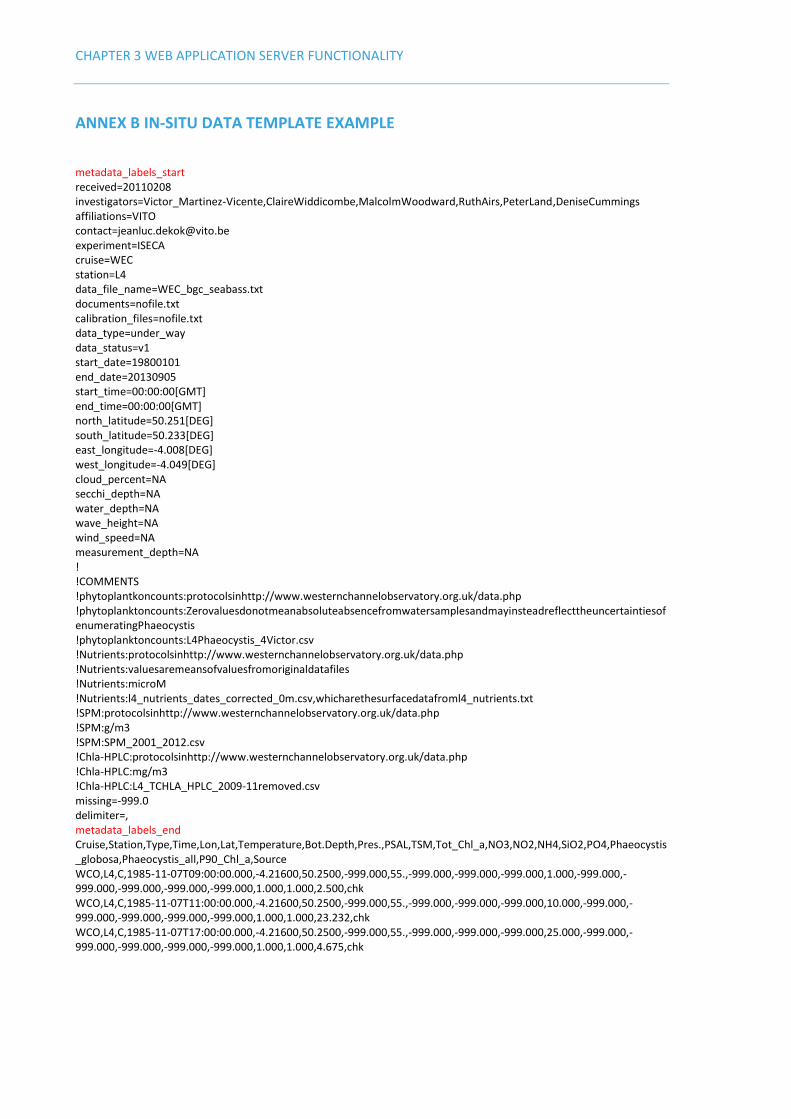
ANNEX B IN-SITU DATA TEMPLATE EXAMPLE
metadata_labels_start received=20110208 investigators=Victor_Martinez-Vicente,ClaireWiddicombe,MalcolmWoodward,RuthAirs,PeterLand,DeniseCummings affiliations=VITO [email protected] experiment=ISECA cruise=WEC station=L4 data_file_name=WEC_bgc_seabass.txt documents=nofile.txt calibration_files=nofile.txt data_type=under_way data_status=v1 start_date=19800101 end_date=20130905 start_time=00:00:00[GMT] end_time=00:00:00[GMT] north_latitude=50.251[DEG] south_latitude=50.233[DEG] east_longitude=-4.008[DEG] west_longitude=-4.049[DEG] cloud_percent=NA secchi_depth=NA water_depth=NA wave_height=NA wind_speed=NA measurement_depth=NA ! !COMMENTS !phytoplantkoncounts:protocolsinhttp://www.westernchannelobservatory.org.uk/data.php !phytoplanktoncounts:ZerovaluesdonotmeanabsoluteabsencefromwatersamplesandmayinsteadreflecttheuncertaintiesofenumeratingPhaeocystis !phytoplanktoncounts:L4Phaeocystis_4Victor.csv !Nutrients:protocolsinhttp://www.westernchannelobservatory.org.uk/data.php !Nutrients:valuesaremeansofvaluesfromoriginaldatafiles !Nutrients:microM !Nutrients:l4_nutrients_dates_corrected_0m.csv,whicharethesurfacedatafroml4_nutrients.txt !SPM:protocolsinhttp://www.westernchannelobservatory.org.uk/data.php !SPM:g/m3 !SPM:SPM_2001_2012.csv !Chla-HPLC:protocolsinhttp://www.westernchannelobservatory.org.uk/data.php !Chla-HPLC:mg/m3 !Chla-HPLC:L4_TCHLA_HPLC_2009-11removed.csv missing=-999.0 delimiter=, metadata_labels_end Cruise,Station,Type,Time,Lon,Lat,Temperature,Bot.Depth,Pres.,PSAL,TSM,Tot_Chl_a,NO3,NO2,NH4,SiO2,PO4,Phaeocystis_globosa,Phaeocystis_all,P90_Chl_a,Source WCO,L4,C,1985-11-07T09:00:00.000,-4.21600,50.2500,-999.000,55.,-999.000,-999.000,-999.000,1.000,-999.000,-999.000,-999.000,-999.000,-999.000,1.000,1.000,2.500,chk WCO,L4,C,1985-11-07T11:00:00.000,-4.21600,50.2500,-999.000,55.,-999.000,-999.000,-999.000,10.000,-999.000,-999.000,-999.000,-999.000,-999.000,1.000,1.000,23.232,chk WCO,L4,C,1985-11-07T17:00:00.000,-4.21600,50.2500,-999.000,55.,-999.000,-999.000,-999.000,25.000,-999.000,-999.000,-999.000,-999.000,-999.000,1.000,1.000,4.675,chk

CHAPTER 3 WEB APPLICATION SERVER FUNCTIONALITY
47
ANNEX C MATLAB MODEL SCRIPT FOR GENERATING MODEL SCENARIOS
A number of scenarios have been modelled to simulate the impact of changes in the terrestrial emissions of nitrogen on the coastal and off-shore eutrophication (see Section 2.4.1). The model has been implemented as Matlab script. The main script EutroShowIndicators35.m asks the modeller to make the following choices:
a. the subregion to model (2Seas areas as defined for the WAS, Seine mouth, Belgian coastal zone, Westerscheldt Estuary or Dutch coastal zone)
b. the indicator to show (salinity, winter DIN, 90th percentile chl-a, OSPAR problem classification or Phaeocystis algae cell count)
c. the general emission scenario to model (pristine without human interference, average for the years 2001-2005 or OSPAR problem limit = pristine + 50 %)
d. the estuary/location for emission reduction if applicable (Scheldt, Seine, Thames or Rhine/Meuse)
e. specific nutrient emission reduction scenario for Scheldt basin: single scenario or all scenarios available (see Section 2.4.1 for details)
f. percentage reduction in nitrogen load (if location chosen under d differs from Scheldt) The script runs a few minutes and then produces a map in Netcdf4 format, which is used for the WAS. A comparison for the 90th percentile chl-a value for the “business-as-usual” scenario (left) and with 70 % reduction in N load of Rhine/Meuse (right) is shown for the Dutch coastal waters here:
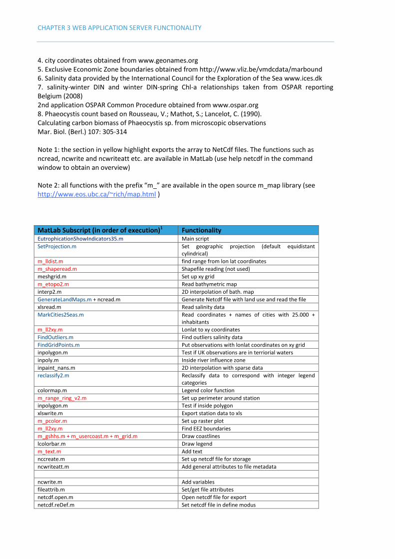
Table 3-1 lists the functions used in the script. Furthermore, the script uses the following open-source software, geodata and publications: 1. m_map http://www.eos.ubc.ca/~rich/map.html 2. INPAINT filling up NaN values based on algorithm by John d'Errico (2006) http://www.mathworks.com/matlabcentral/fileexchange/4551 3. Global Self-consistent Hierarchical High-Resolution (GSHHS) Coastline data http://www.ngdc.noaa.gov/mgg/shorelines/gshhs.html
CHAPTER 3 WEB APPLICATION SERVER FUNCTIONALITY
4. city coordinates obtained from www.geonames.org 5. Exclusive Economic Zone boundaries obtained from http://www.vliz.be/vmdcdata/marbound 6. Salinity data provided by the International Council for the Exploration of the Sea www.ices.dk 7. salinity-winter DIN and winter DIN-spring Chl-a relationships taken from OSPAR reporting Belgium (2008) 2nd application OSPAR Common Procedure obtained from www.ospar.org 8. Phaeocystis count based on Rousseau, V.; Mathot, S.; Lancelot, C. (1990). Calculating carbon biomass of Phaeocystis sp. from microscopic observations Mar. Biol. (Berl.) 107: 305-314 Note 1: the section in yellow highlight exports the array to NetCdf files. The functions such as ncread, ncwrite and ncwriteatt etc. are available in MatLab (use help netcdf in the command window to obtain an overview) Note 2: all functions with the prefix “m_” are available in the open source m_map library (see http://www.eos.ubc.ca/~rich/map.html )
MatLab Subscript (in order of execution)1 Functionality EutrophicationShowIndicators35.m Main script
SetProjection.m Set geographic projection (default equidistant cylindrical)
m_lldist.m find range from lon lat coordinates
m_shaperead.m Shapefile reading (not used)
meshgrid.m Set up xy grid
m_etopo2.m Read bathymetric map
interp2.m 2D interpolation of bath. map
GenerateLandMaps.m + ncread.m Generate Netcdf file with land use and read the file
xlsread.m Read salinity data
MarkCities2Seas.m Read coordinates + names of cities with 25.000 + inhabitants
m_ll2xy.m Lonlat to xy coordinates
FindOutliers.m Find outliers salinity data
FindGridPoints.m Put observations with lonlat coordinates on xy grid
inpolygon.m Test if UK observations are in terriorial waters
inpoly.m Inside river influence zone
inpaint_nans.m 2D interpolation with sparse data
reclassify2.m Reclassify data to correspond with integer legend categories
colormap.m Legend color function
m_range_ring_v2.m Set up perimeter around station
inpolygon.m Test if inside polygon
xlswrite.m Export station data to xls
m_pcolor.m Set up raster plot
m_ll2xy.m Find EEZ boundaries
m_gshhs.m + m_usercoast.m + m_grid.m Draw coastlines
lcolorbar.m Draw legend
m_text.m Add text
nccreate.m Set up netcdf file for storage
ncwriteatt.m Add general attributes to file metadata
ncwrite.m Add variables
fileattrib.m Set/get file attributes
netcdf.open.m Open netcdf file for export
netcdf.reDef.m Set netcdf file in define modus

CHAPTER 3 WEB APPLICATION SERVER FUNCTIONALITY
49
netcdf.inqVar.m Request information about variable
netcdf.renameatt.m Relabel attribute
netcdf.close.m Close netcdf file
ncdisp.m Show content summary of netcdf file in MatLab command window
Table 3-1 Overview MatLab scripts used in main script (blue = custom scripts, red = m_map library).
Other auxiliary function are customized scripts with the following functions:
DifMap2.m: shows the difference between two maps
CombineNetcdf.m: combines two maps with different variables in a single map
GenerateEEZboundaries: translates shape file with EEZ boundaries into grid points
ShowNetcdf2: visualizes map in netcdf format
GenerateLandMaps: uses GSHHS coastal database(http://www.ngdc.noaa.gov/mgg/shorelines/gshhs.html ) with world coastlines to obtain lon-lat coordinates and generates land map (outside model)
RefineAtmosphericData.m: The script codes are available upon request.
CHAPTER 3 WEB APPLICATION SERVER FUNCTIONALITY
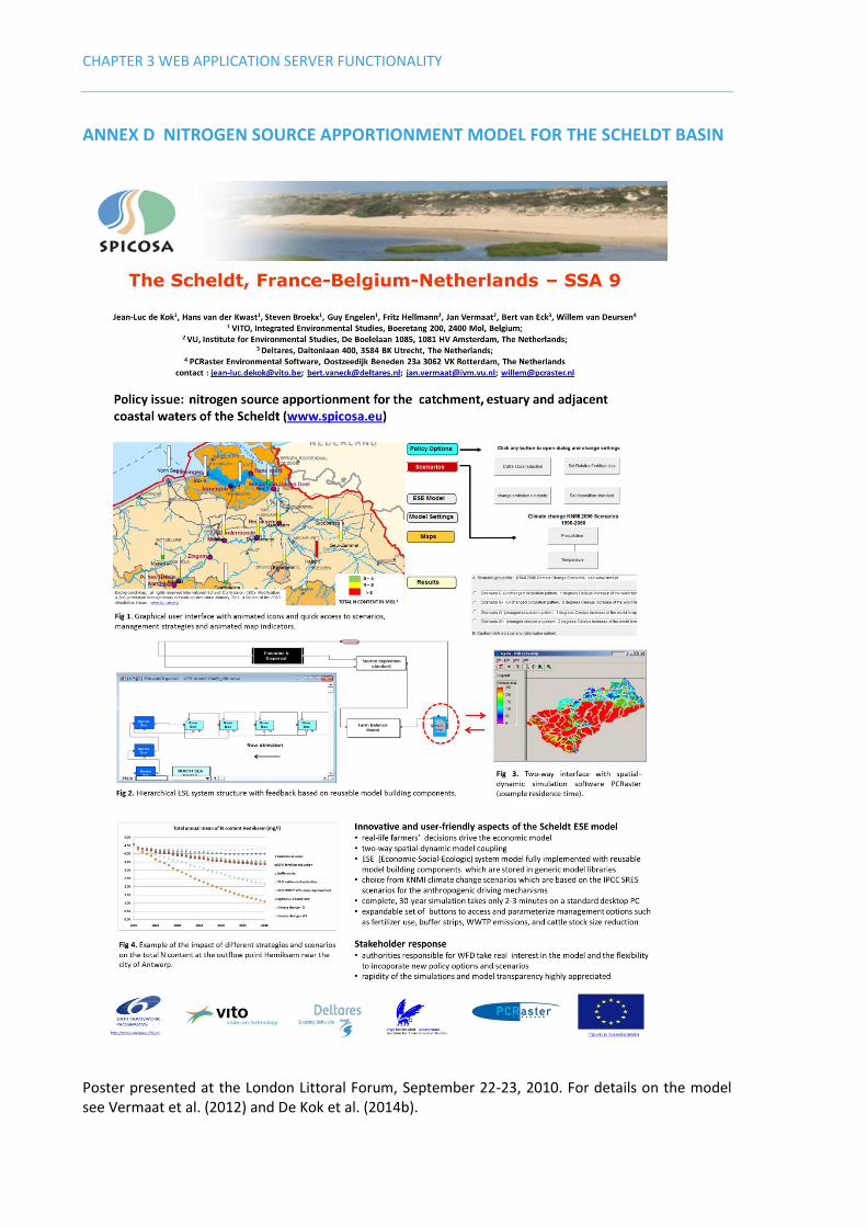
ANNEX D NITROGEN SOURCE APPORTIONMENT MODEL FOR THE SCHELDT BASIN
Poster presented at the London Littoral Forum, September 22-23, 2010. For details on the model see Vermaat et al. (2012) and De Kok et al. (2014b).