LARS Information Note 111572

Pattern Recognition: A Basis for

Remote Sensing Data Analysis'

by

Philip H. Swain2

0 Ni

M HM f

N X

I-'. !: WC txjO.3.4

t4qLn :o en

0

0 L-rn

k'l

ow..3

aA I--II.-

1W1

Or/i*s,4,D; S

N0co

0~ (N:a

OID SW>

En

-4

-A

INTRODUCTION

Pattern recognition plays a central role in numerically

oriented remote sensing systems. It provides an automatic

procedure for deciding to which class any given ground resolu-

tion element should be assigned. The assignment is made in such

a manner that on the average correct classification is achieved.

This information note describes briefly the theoretical basis

for the pattern-recognition-oriented algorithms used in LARSYS,

the multispectral data analysis software system developed by

the Laboratory for Applications of Remote Sensing (LARS).

Figure 1 shows a model of a general pattern recognition

system. In the LARS context the receptor or sensor is usually

a multispectral scanner. For each ground resolution element

the receptor produces n numbers or measurements corresponding to

the n channels of the scanner. It is convenient to think of

the n measurements as defining a point in n-dimensional Euclidean

space which is referred to as the measurement space. Any particular

measurement can be represented by the vector:

'Research reported here was supported by NASA Grant NGL 15-005-112.

2 Program Leader for Data Processing and Analysis Research, LARS.

Reproduced by

NATIONAL TECHNICALINFORMATION SERVICE

US Department of CommerceSpringfield, VA. 22151

.4'I

11

li

III

https://ntrs.nasa.gov/search.jsp?R=19730008457 2018-06-17T10:11:56+00:00Z

-2-

+ +vector in vector inmeasurement feature spacespace

Figure 1. A Pattern Recognition System

receptor(sensor)

Xi

X2

:n

decisionmaker

result

Figure 2. A Simplified Model of aPattern Recognition System

,aur(pattern

-3-

xl

x2

Xn

The feature extractor transforms the n-dimensional measure-

ment vector into an n'-dimensional feature vector. In LARSYS,

this consists simply of selecting a subset of the components of

the measurement vector, but much more complex transformations

are possible (see, for example, Ready et al, 1971).

The decision maker in Figure 1 performs calculations on the

feature vectors presented to it and, based upon a decision rule,

assigns the "unknown" data point to a particular class.

For the present, it will be sufficient to simplify the

model to that shown in Figure 2. The vector X may subsequently

be referred to as either a measurement vector ora feature vector.

DISCRIMINANT FUNCTIONS: QUANTIFYING THE DECISION PROCEDURE

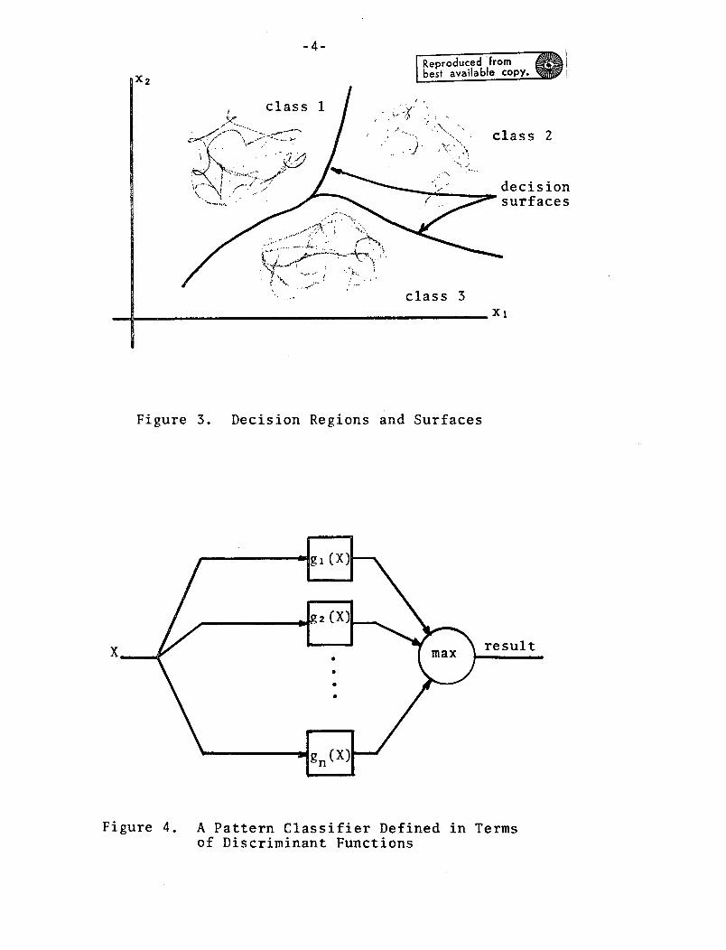
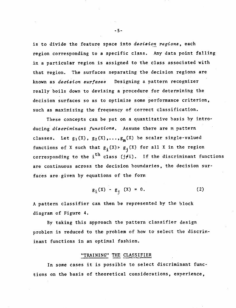
Patterns arising in remote sensing problems exhibit some

randomness due to the randomness of nature. As an example, one

cannot in general expect the vector of measurements corresponding

to a particular ground resolution element from one part of a

wheat field to correspond exactly to the vector corresponding to

a ground resolution element from another part of the field.

Rather, vectors from the same class tend to form a "cloud" of

points as shown in Figure 3. The job of the pattern classifier

-4-Reproduced from I

Ibest available copy. i

class 2

decisionsurfaces

class 3XI

Figure 3. Decision Regions and Surfaces

Figure 4. A Pattern Classifier Defined in Termsof Discriminant Functions

X 2

-5-

is to divide the feature space into decision regions, each

region corresponding to a specific class. Any data point falling

in a particular region is assigned to the class associated with

that region. The surfaces separating the decision regions are

known as decision Burfaces, Designing a pattern recognizer

really boils down to devising a procedure for determining the

decision surfaces so as to optimize some performance criterion,

such as maximizing the frequency of correct classification.

These concepts can be put on a quantitative basis by intro-

ducing discriminant functions. Assume there are m pattern

classes. Let gl(X), g2 (X),...,gm(X) be scalar single-valued

functions of X such that gi(X)> gj(X) for all X in the region

corresponding to the ith class (j'i). If the discriminant functions

are continuous across the decision boundaries, the decision sur-

faces are given by equations of the form

gi(X) - gj (X) = O. (2)

A pattern classifier can then be represented by the block

diagram of Figure 4.

By taking this approach the pattern classifier design

problem is reduced to the problem of how to select the discrim-

inant functions in an optimal fashion.

"TRAINING" THE CLASSIFIER

In some cases it is possible to select discriminant func-

tions on the basis of theoretical considerations, experience,

-6-

or perhaps even intuition. More commonly the discriminant

functions are based upon a set of training patterns. Training

patterns which are typical of those to be classified are "shown"

to the classifier together with the identity of each patter; and

based on this information the classifier establishes its dis-

criminant functions gi(X), i=l, 2, ..., m.

Example: Consider a two-dimensional, two-class problem in

which the discriminant functions are assumed to have the form

gl(X) = all xl + a1 2 x2 + bl

g2 (X) = a2 1 X1 + a2 2 x2 + b2

Then gl(X) - g2(X) = 0 is the equation of a straight line

dividing the xl, x2 plane. Given a set of training patterns,

how should the constants all, al2, bl, etc. be chosen? It can

be proven that if the training patterns are indeed separable

by a straight line,then the following procedure will converge

(Nilsson, 1965):

Initially select a's and b's arbitrarily. For

example let

all ' a1 2 - b1 = 1(4)

a 2 1 = a 2 2 = b 2 = -1

Then take the first training pattern (say it is from Wl,

i.e., from class 1) and calculate gl(X) and g2 (X). If

g 1 (X) > g2 (X) the decision is correct; go on to the next

training sample. If gl(X) < g2(X) a wrong decision would

-7-

be made. In this case alter the coefficients so as

to increase the discriminant function associated with

the correct class and decrease the discriminant func-

tion associated with the incorrect class. If X is from

wl but W2 was decided, letI I

al 1 = al 1 + aCXl a2 a 21 - aXl

I !al 2 = a1 2 + aX2 a22 = a22 - aX2 (5)

! !

bl = bl- + a b2 = b2 -a

where a is a convenient positive constant. If X is from

a2 but w, was decided, change the signs in Eq. (5) so as

to increase g2 and decrease gi. Then go on to the next

training pattern. Cycle through the training patterns until

all are correctly classified.

Suggestion: Design and work out a numerical example to

illustrate the training process described above. Assume two

classes, two dimensions, and two training patterns per class.

THE STATISTICAL APPROACH

Remote sensing is typical of many practical applications of

pattern recognition for which statistical methods are appropriate

in the following respects:

-The data exhibit many incidental variations (noise) which

tend to obsure differences between the pattern classes.

*There is often uncertainty, however small, concerning the

true identity of the training patterns.

-The pattern classes of interest may actually overlap in

the measurement space (may not always be discriminable),

-8-

suggesting the use of an approach which leads to decisions

which are "most likely" correct.

Statistical pattern recognition techniques often make use

of the probability density functions associated with the

pattern classes (including the approach to be described here).

However, the density functions are usually unknown and must be

estimated from a set of training patterns. In some cases, the

form of the density functions is assumed and only certain para-

meters associated with the functions are estimated. Such methods

are called "parametric." Methods for which not even the form

of the density functions is assumed are called "nonparametric."

The parametric case requires more a priori knowledge or some

basic assumptions regarding the nature of the patterns. The non-

parametric case requires less initial knowledge and fewer assump-

tions but is generally more difficult to implement.

Let there be m classes characterized by the conditional

probability density functions

p(XI Wi) i = 1, 2, ... , m. (6)

The function p(Xlwi ) gives the probability of occurrence of

pattern X,given that X is in fact from class i.

An important assumption in the LARSYS algorithms is that

the p(X[wi) are each multivariate gaussian (or normal) distri-

butions. This is a parametric assumption which leads to a form

of classifier which is relatively simple to implement. Under this

assumption, a mean vector and covariance matrix are sufficient to

-9-

characterize the probability distribution of any pattern class.

Returning to the problem of how to specify the discriminant

functions, an approach based on statistical decision theory is

taken. A set of loss functions is defined

X(ilj) i = 1, 2, .. , m; j = 1, 2, ..., m (7)

where X(ilj) is the loss (or cost) incurred when a

pattern is classified into class i when it is actually from

class j.

If the pattern classifier is designed so as to minimize the

average (expected) los88, then the classifier is said to be Bayes

optimaZ. This is the criterion to be used in specifying the

classification algorithm.

For a given pattern X, the expected loss resulting from

the decision Xcwi is given by1

mLx(i) = X(ilj)p(bjlX) (8)

j=l

where p(wj IX) is the probability that a pattern X is from class

j. Applying Bayes' rule, i.e.,

p(X,wj) = p(XIwj)p(j) = p(wjIX) p(X) (9)

the expected loss can be written as

mLx(i) = Z X(ilj)p(Xwj)p(Wj p (10)

j=l j iP

where p(wj) is the a priori probability of m.

Note that minimizing Lx(i) with respect to i is the same

as maximizing -Lx(i). Thus a suitable set of discriminant

-10-

functions is

gi(X) ' -L x(i) i = 1, 2, ..., m. (11)

A simple (and reasonable) loss function is

X(ilj) o i = j(12)

X(iJj) 2 1 i ' j

(zero loss for correct classification, unit loss for any error).

Then

'Igi(X) = - Z p(XjW)p(W )/p(X) (13)

j=1 3 3j i

Here and at several points later in this paper it will be con-

venient to make use of the following fact: from any set of

discriminant functions, another set of discriminant functions can be

formed by taking the same monotonic function of each of the

original discriminant functions. For example, if

gi(X):, i = 1, 2, ..., m

is a set of discriminant functions, then so are the sets

I

gi(x) = gi(X) + constant i = 1, 2, ..., m

and

. .

gi(X) = 1og[gi(X)] i = 1, 2, ... , m.

Examining (13) note that p(X) is not a function of i so it

is just as well to maximize

-11-

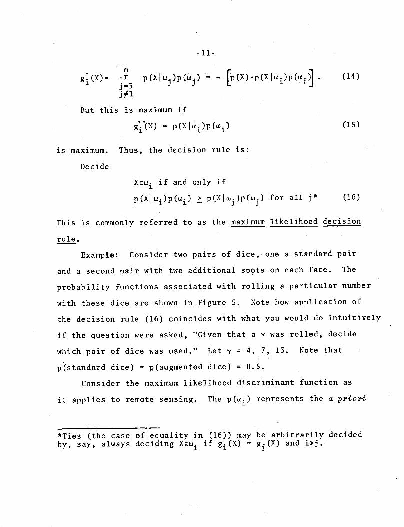
~~~~~~~~~(X)-pXli)(Xi . W (14)gi(X)= -E p(Xlj)p(j) = X)- (XIW)P(i (14)i ~j=l J J

j-1jil

But this is maximum if

gi(X) = P(Xlki)p(%i) (15)

is maximum. Thus, the decision rule is:

Decide

X¢wi if and only if~~~~~~~~~~~~~16

p(Xloi)p(wi) > p(XljWj)p(W

j) for all j* (16)

This is commonly referred to as the maximum likelihood decision

rule.

Example: Consider two pairs of dice, one a standard pair

and a second pair with two additional spots on each face. The

probability functions associated with rolling a particular number

with these dice are shown in Figure 5. Note how application of

the decision rule (16) coincides with what you would do intuitively

if the question were asked, "Given that a y was rolled, decide

which pair of dice was used." Let y = 4, 7, 13. Note that

p(standard dice) = p(augmented dice) = 0.5.

Consider the maximum likelihood discriminant function as

it applies to remote sensing. The p(wi) represents the a priori

*Ties (the case of equality in (16)) may be arbitrarily decidedby, say, always deciding XEwi if gi(X) = gj(X) and i>j.

- 1 2 -

a)u

.H

r~~~~~

r'

ad jIt I

a.)

Xr J

L- 1 1

'

L _I

©.0

'-4EH

o-i 0

4-4(j

'-4 r0,

o .

p,)

u ua

*14

co *,10

rI -

.r4

L1i 4

?n tn t e (n

-13-

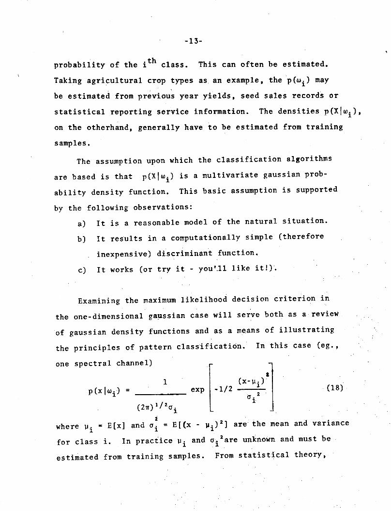
thprobability of the i t h class. This can often be estimated.

Taking agricultural crop types as an example, the p(wi) may

be estimated from previous year yields, seed sales records or

statistical reporting service information. The densities p(X[wi),

on the otherhand, generally have to be estimated from training

samples.

The assumption upon which the classification algorithms

are based is that p(Xlwi) is a multivariate gaussian prob-

ability density function. This basic assumption is supported

by the following observations:

a) It is a reasonable model of the natural situation.

b) It results in a computationally simple (therefore

inexpensive) discriminant function.

c) It works (or try it - you'.11 like it!).

Examining the maximum likelihood decision criterion in

the one-dimensional gaussian case will serve both as a review

of gaussian density functions and as a means of illustrating

the principles of pattern classification. In this case (eg.,

one spectral channel) r

1 (X -. i ) x~p(xIw) = exp -1/2 (18)

(2i2

where pi = E[x] and ai = E[(x - i ) 2] are the mean and variance1 1~a

for class i. In practice pi and oi2are unknown and must be

estimated from training samples. From statistical theory,

-14-

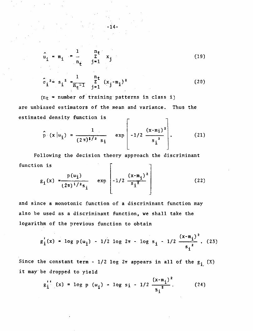
^' 1U

im = m

n tn t

ntj=l.j=l

X. (19)

^.2=52= 1 'n t2= Si2 = j (xj- i) 21 i -r E (X. -m.)i nt- j=l

(nt = number of training patterns in class i)

are unbiased estimators of the mean and variance. Thus the

estimsated rdenscitv func.tian ic

20)

VZO L. L il U . U UVX HZ L7 L~ a v XLLJL% LJL L_

,,1 .(x-mi) 2p(x i (2)/ si exp -1/2 (21

1 (2lr.f)1/2 Si 2(~~~~~~~~~2 I

Following the decision theory approach the discriminant

function is r 1

1)

P(wi)gi (x) = - )/ 2 s iCZ2f) 1/2s.

exp -1/2

and since a monotonic function of a discriminant function may

also be used as a discriminant function, we shall take the

logarithm of the previous function to obtain

~~~~~~~~~~~, (x-mi)2gi(x) = log p(wi) - 1/2 log 2w - log si - 1/2 . (23)

si

Since the constant term - 1/2 log 2w appears in all of the gi, (X)

it may be dropped to yield

gI Ix) (XM log P (i) log si - 1/2i) 2gi' (x) = log p (Wi) - log si - 1/2 ( )2

(22)

q

(24)

-15-

Thus the decision rule becomes:

Decide X wi if and only if1

(x-mi)22(x-m.) 2

log p(Wi)-log si-1/2 1 > log p2( )-log s-1/2 (25)s1

The one dimensional case just described serves to

illustrate the Bayes decision rule for gaussian-statistics.

In the two dimensional case

x l

x = ., (26)

x 2 jand

1p(Xlwi) =

27(ail1l ai2 2

(27)2 .1/2 (il12)

2 -(xl- Vil)

aill

2.il 2 (Xl "il) (X2-i2)

(aill ' Oi22) 1/

2

(x2-Pi2)2

°i2,2

expt- 1/2

1-

2

1 °i 2

aOill °i22

where

il= E [x 1 Ii], vi2 = E [x2 1 Wi]j,k 1,2 (28)

oijk = E[(xj-p ij)(Xk-iklJ i] i = 1,2,...R

This is a formidible expression, but by defining a mean vector

and covariance matrix

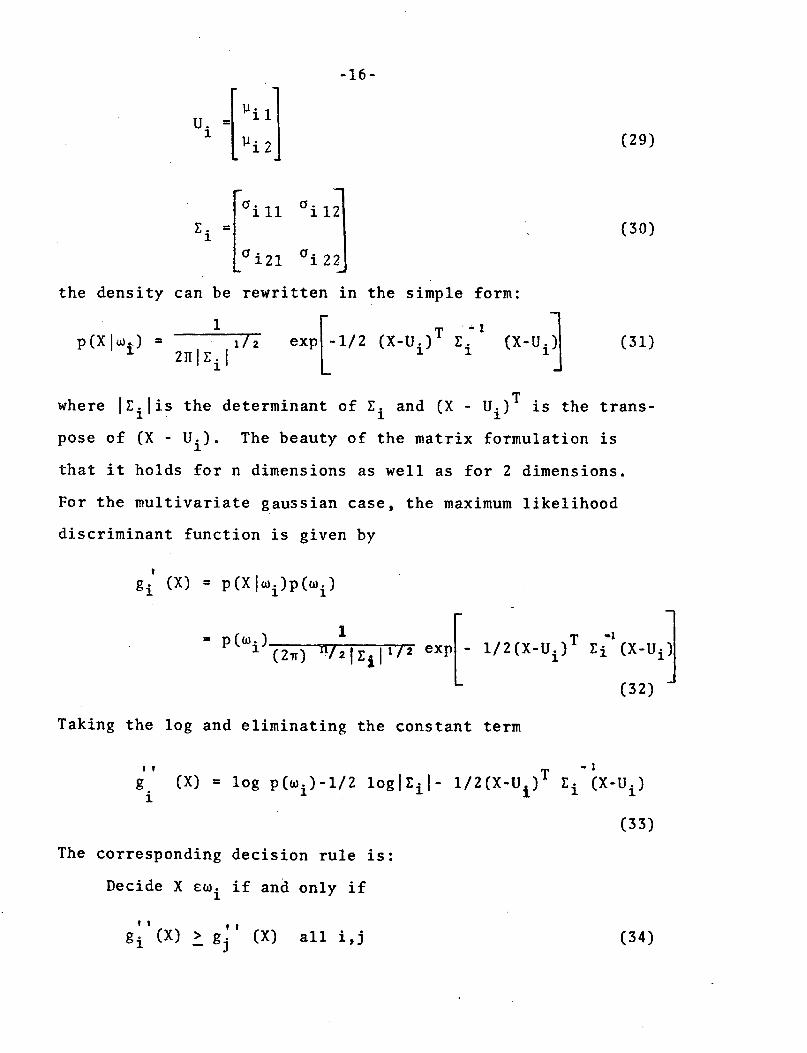
-16-

tU.lu i 2 (29)

12(30)

i 21 i 22

the density can be rewritten in the simple form:

1 7T -z.p(X[~

i)= 1/2 ~ ~ ~ i)P(XWj) 1j2 exp (1/2 (X-U) . (X-Ui) (31)

where Itilis the determinant of ri

and (X - Ui)T is the trans-

pose of (X - Ui). The beauty of the matrix formulation is

that it holds for n dimensions as well as for 2 dimensions.

For the multivariate gaussian case, the maximum likelihood

discriminant function is given by

gi (X) = p(XIli)P(wi)

= 1i(2w) / 2 1zt[ 1/2 exp1 1/2 (X-Ui)T ci (X-U i

(32)

Taking the log and eliminating the constant term

Tg (X) = log p(wi)-1/2 log[Ei l- 1/2(X-U)T Ei (X-Ui )

i

(33)

The corresponding decision rule is:

Decide X ewi if and only if

gi (X) > gj (X) all i,j (34)

-17-

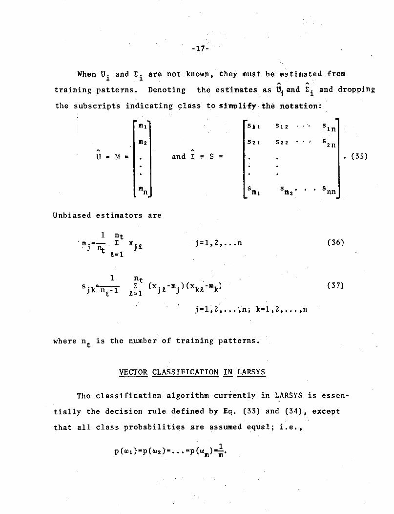
When Ui and Ei are not known, they must be estimated fromA A

training patterns. Denoting the estimates as Uiand Ei and dropping

the subscripts indicating class to simplify the notation:

.ml .Sl . S 512 - Sin

M2 S21 522 2 s2n

U = M = . and Z S= S = . . .(35)

mn nj Sn2

. Snn

Unbiased estimators are

1 nt= xEj j=l,2,... n (36)

nt 1

1 n tS~ ~~~. f X M ( 37)

Sjk-nt'l 1=1 ( xj i -mj) fxkl-~k) (7

j=l,2,...,n; k=1,2,...,n

where nt is the number of training patterns.

VECTOR CLASSIFICATION IN LARSYS

The classification algorithm currently in LARSYS is essen-

tially the decision rule defined by Eq. (33) and (34), except

that all class probabilities are assumed equal; i.e.,

p(Wl)=P(W2)=...=P(Wm)'1

-18-

The required mean vectors and covariance matrices are computed

from training patterns by the statistics processor. The clas-

sification processor computes the gi(X), i-l,2,...m for every

data vector in the area to be classified. For each vector the

class decided and the value of the discriminant function com-

puted for that class are written on magnetic tape for later use

by the results display processor.

Inevitably there are points in the area classified which

do not belong to any of the classes defined by the training

samples. In agricultural settings such points might be from

roads, fence lines, farmsteads, and the like. The classification

procedure necessarily assigns these points to one of the train-

ing classes, but typically they may be expected to yield very

small discriminant values. The later fact can be utilized to

detect them, as will now be described.

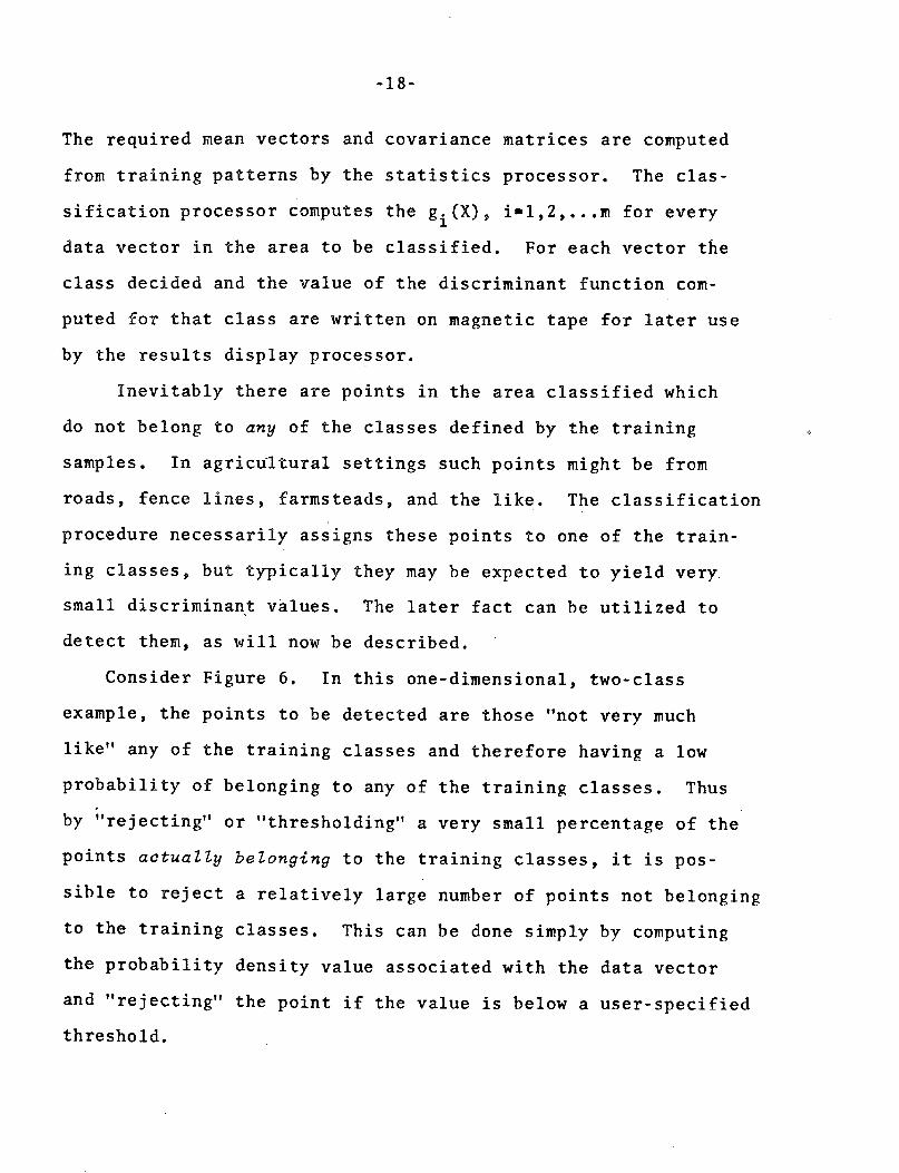
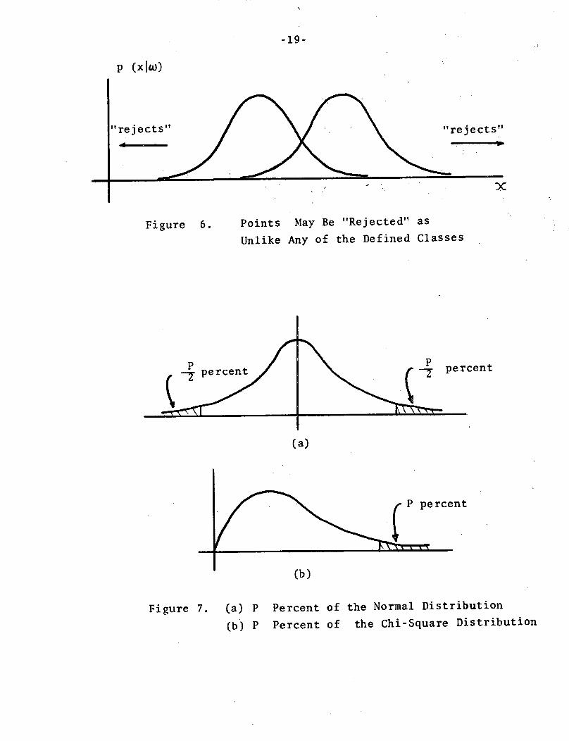
Consider Figure 6. In this one-dimensional, two-class

example, the points to be detected are those "not very much

like" any of the training classes and therefore having a low

probability of belonging to any of the training classes. Thus

by "rejecting" or "thresholding" a very small percentage of the

points actuaZZy belonging to the training classes, it is pos-

sible to reject a relatively large number of points not belonging

to the training classes. This can be done simply by computing

the probability density value associated with the data vector

and "rejecting" the point if the value is below a user-specified

threshold.

-19-

p (x 1w)

"rejects"Id~

X

Figure 6.

P-1- percent

Points May Be "Rejected" as

Unlike Any of the Defined Classes

- percent-7 percent

(a)

P percent

.I _ _ I II

(b)

Figure 7. (a) P Percent of the Normal Distribution

(b) P Percent of the Chi-Square Distribution

.it

__l

-20-

But this can be accomplished just as well using the discrim-

inant values stored as part of the classification result. If X

is n-dimensional and normally distributed then the quadratic

form

(X-Ui)T E ' (X-Ui) (38)

has a chi-square distribution with n degrees of freedom

(Cn(X2)), Therefore to threshold, say, P percent of the normal

distribution shown in Figure 7a, it is just as well to threshold

P percent of the chi-square distribution of (X - Ui ) T E.(X - Ui).

This quadratic form is related to gi(X) in the following manner:

(X-Ui) i (X-Ui) = -2gi(X) + 2bi (39)

where

bi = log p(wi) - 1/2 log ]Ei[ (40)

Thus, every point for which

-2gi(X) + 2bi>(X2 for which Cn(x2 ) = P/100) (41)

is rejected or thresholded. Note that a different threshold

value may be applied to each class.

FEATURE SELECTION

Problem: Given a set of N features (eg., multispectral

scanner channels), find a subset consisting of n channels which

provides an optimal trade-off between classification costs

(complexity and time for computation) and classification accuracy.

-21-

Ideally, one would like to solve this problem by computing

the probability of misclassification associated with each

n-feature subset and then selecting the one giving best per-

formance. However, it is generally not feasible to perform the

required computations. Even under the simplifying assumption

of normal statistics, numerical integration is required which,

in the multidimensional case, is impractical to carry out. To

see this, consider that

( N

(42)\ n) n!(N-n)! (42)

subsets of features must be evaluated. Thus, for example, to

select the best 4 out of 12 available features requires

l2= 12! = (43)

4' 4! 8!

integrations in 4-dimensional space. Even on the fastest

computers, such computations would be prohibitive. Alternative

methods must be found for feature selection.

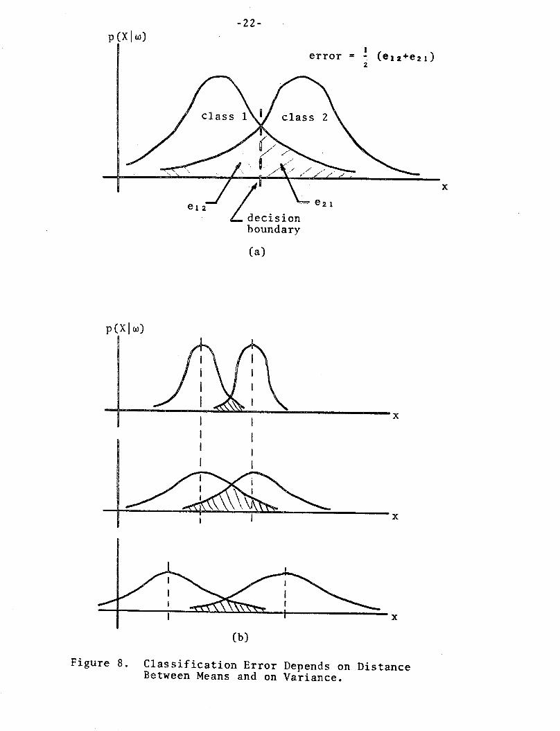
From Figure 8, the probability of error (proportional to the

shaded area) can be seen to be a function of the "normalized

distance" between the classes. That is, the error depends upon

both the distance between the means as well as the variance of each

class. The greater the "distance" the smaller the probability

of error.

One measure of the distance between classes is known as

divergence. Divergence is defined in terms of the Zikelihood ratio

-22-

error = - (el2+e2 1)2

I J I \X" e2! /el2decisionboundary

(a)

p(XIW)

I xi I

I~~~~~~~~~~~~

I iII I I

I I

I I

x

(b)

Figure 8. Classification Error Depends on DistanceBetween Means and on Variance.

-23-

L()-p(Xfwi) :(44)ij p(XIWj)

which is a measure or indication of the separability of the

densities at X. The logarithm of the likelihood ratio provides

an equivalent indication of the separability of the densities:

Lij (X) = log Lij(X) = log p(Xwii) - log p(XIj) (45)

Divergence is defined* as

D(i,jlcl, C2,.¢n )=-

E[LOj(X) I i ] - E[Lj(X)IWj] (46)

for channels cl, c2,...,cn where

E[Lij (X)i)] A jLl(X) (X i ) dX (47)ij ~ ~~~ JX .,.

Divergence has the following properties:

1) D(i,jcl, ....cn ) > 0 for non-identical distributions

2) D(i,ilcl,...,cn ) = 0

3) D(i,j cl,...,cn) = D(j,ifcI, C2,...c

n

) (48)

4) Divergence is additive for independent featuresn

D(i,jcl, c2,....,cn) = E D(i,jlck )

k=l5) Adding new features never decreases the divergence, i.e.,

D(i,jlcl,...,cn) < D(i,jc ,...,cn,cn+l)

Divergence is defined for any two density functions. Inthe

See for instance Kullback, 1959.

-24-

case of normal variables with unequal covariance matrices, it can

be shown that

D(i,jlci,...,cn ) = 1/2 tr[(i-Ej)(Ej l-l)]il ... Pcn1 J j

(49)+1/2 tr[(E 1 +E-l)(Ui-U) U- Uj)T] I

where tr[A] (trace A) is the sum of the diagonal elements of A.

Divergence is a measure of the dissimilarity of two distri-

butions and thus provides an indirect measure of the ability

of the classifier to discriminate successfully between them.

Computation of this measure for n-tuples of the available

features provides a basis for selecting an optimal set of n

features.

Divergence is defined for two distributions. Remote sens-

ing problems usually involve m > 2 classes. Several strategies

have been suggested and used for feature selection in the multi-

class case.

One strategy is to compute the average divergence over

all pairs of classes and select the subset of features for

which the average divergence is maximum. That is, maximize with

respect to all n-tuples

2 m-l mDAVE(elIc2, .. Cn) - Z Z D(i,j cl,pc2,..ICn)

e(m-1) i=l j=i+l(50)

While this strategy is certainly reasonable there is no guarantee

that it is optimal. It must be used with care. For instance, a

single pairwise divergence, i.e., a single term in (50), if it

-25-

were large enough, could make the average very large. This is

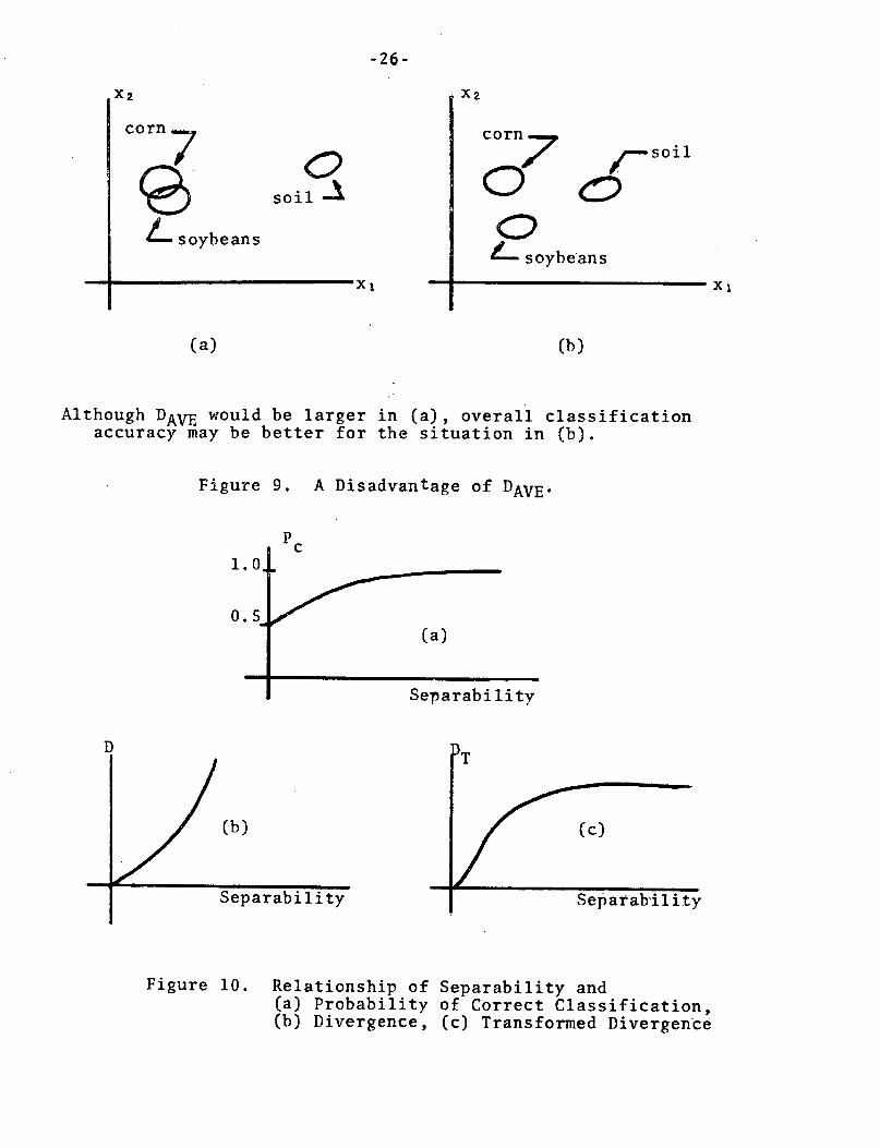
illustrated in Figure 9. So in the process of ranking feature

combinations by DAVE, it is agood idea to examine each of the

pairwise divergences as well.

Another strategy is to maximize the minimum pairwise diver-

gence, i.e., to select the feature combination which does the

best job of separating the hardest-to-separate pair of classes.

This is not a Bayesian (minimum risk) strategy, but it is cer-

tainly a reasonable strategy for many remote sensing problems.

The problem illustrated in Figure 9 is amplified by the

following fact: As the separability of a pair of classes

increases, the pairwise divergence also increases without limit--

but the probability of correct classification saturates at 100

percent (see Figure 10). A modified form of the divergence,

referred to as the "transformed divergence," DT, has a

behavior more like probability of correct classification:

DT = 2[1-exp(-D/8)] (51)

where D is the divergence discussed above. The saturating

behavior of this function (see Figure 10) reduces the effects

of widely separated classes when taking the average over all

pairwise separations. DAVE based on transformed divergence

has been found a much more reliable criterion for feature

selection than the DAVE based on "ordinary" divergence.

-26-

X 2

corn7

L soybeans'/ soybeans

sOilsoil A-

;1

X2

corn,

O7/--soil

<f)O

- soybeans

x l

(a) (b)

Although DAVE would be larger in (a), overall classificationaccuracy may be better for the situation in (b).

Figure 9. A Disadvantage of DAVE.

1.0.

0. 5

Pc

(a)

Separability

(b)

ty

Figure 10. Relationship of Separability and(a) Probability of Correct Classification,(b) Divergence, (c) Transformed Divergence

-27-

CLUSTERING

Clustering is a data analysis technique by which one

attempts to determine the "natural" or "inherent" relationships

in a set of observations or data'points. It is sometimes refer-

red to as unsupervised classification because the end product

is generally a classification of each observation into a "class"

which has been established by the analysis procedure, based on

the data, rather than by the person interested in the analysis.

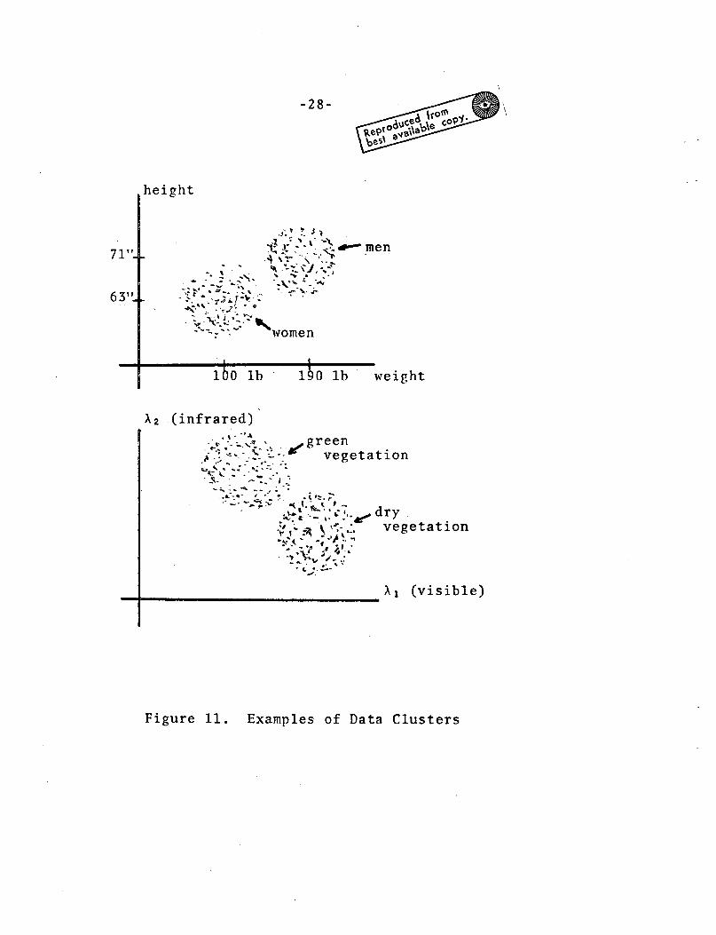
To get an intuitive idea of what is meant by natural or

inherent relationships in a set of data, consider the examples

shown in Figure 11. If one were to plot height versus weight

for a random sampling of students, without regard to sex, on a

college campus, it is likely that two relatively distinct clusters

of observations would result, one corresponding to the men in

the sample (heavier and taller) and another corresponding to the

women (lighter and shorter). Similarly, if the spectral reflec-

tance of vegetation in a visible wave band were plotted against

reflectance in an infrared wave band, dry vegetation and green

vegetation could be expected to form discernible clusters.

If the data of interest never involved more than two

attributes (measurements or dimensions), cluster analysis

might always be performed by visual evaluation of two-dimensional

plots such as those in Figure 11. But beyond two or possiblythree dimensionsvisualanalysis is impossible. For such cases,

three dimensions,·visual analysis is impossible. For such cases,

-28-

height

71" $ . men

"':" -women

lbO lb lbO lb weight

X2 (infrared)

X -..· green

_.-. ,, .: -.-. - :vegetation

-!_ __. ~ ' -~. .° . tt

- ,' ~1' .. .,dry< @I, ~vegetation

- (visible) -

X1 (visible)

Examples of Data ClustersFigure 11.

-29-

it is desirable to have a computer perform the cluster

analysis and report the results in a useful fashion.

Why is clustering a useful analysis tool? Clustering has

been applied as a means of data compression (eg., for transmis-

sion or storage) and for the purpose of determining differenti-

ating characteristics in complex data sets (eg., in numerical

taxonomy). An increasingly important application is unsuper-

vised classification, in which the clustering algorithm determines

the classes based on the clustering tendencies in the data.

The results of such a classification are useful if the "cluster

classes" can be interpreted as classes of interest to the data

analyst.

With respect to LARSYS, the greatest use of cluster analysis

has been for the purpose of assuring that the data used to

characterize the pattern classes do not seriously violate the

assumption of gaussian statistics. In general it may be expected

that each distinct cluster center will correspond to a mode in

the distribution of the data. Therefore, by defining a pattern

subclass for each cluster center, the possibility of multimodal

(and hence definitely non-gaussian) class distributions is

essentially eliminated.

The reader interested in the many possible ways of defining

clustering. in quantitative terms may consult the references

(Wacker and Landgrebe, 1971; Hall, 1965). Essentially, the

definition of a clustering algorithm depends on the specification

of two distance measures: a measure of distance between data

-30-

points or individual observations; and a measure of distance

between groups of observations. Figure 12 is a block diagram

for a typical clustering algorithm (including the LARSYS

algorithm). The point-to-point distance measure is used in the

step labelled "Assign each vector to nearest cluster center."

The distance between groups of points (clusters, in this case)

is calculated in the step "Compute separability information."

Euclidean distance, the most familiar point-to-point dis-

tance measure, is defined for two n-dimensional points or

vectors X and Y as follows;

Euclidean distance: D =[ I (xi-yi)2] / (52)

Several alternatives are available as candidate measures

of distance between clusters, each having its peculiar advantages

and disadvantages. One possibility is the

divergence or transformed divergence used for feature selection.

In LARSYS, a measure called "Swain-Fu distance" has been imple-

mented, which compares the separation of cluster centers to the

dispersion of the data in the clusters. The dispersion of the

data in a cluster is measured in terms of the "ellipsoid of

concentration" associated with the cluster.

Ellipsoid of concentration: Let the random vector X have

a distribution with mean vector U and covariance matrix E=lai].

If Z is another random vector uniformly distributed over the

volume of the ellipsoid given by

Q(Z)= I (zi-u i ) ( zj

- uj

) = n+2 (3)i=l j=l 1 .(

-31-

Clustering AlgorithmFigure 12.

-32-

where n is the number of components in Z, and E ijj is the

cofactor of aij, then Z also has zero mean and covariance matrix

E. The ellipsoid Q is called the ellipsoid of concentration

of the distribution of X.

Q as given by equation (53) is the ellipsoid of concentration

of any distribution with mean U and covariance E and in particular

serves as a geometrical characterization of the concentration

(or equivalently, thedispersion) of these distributions.

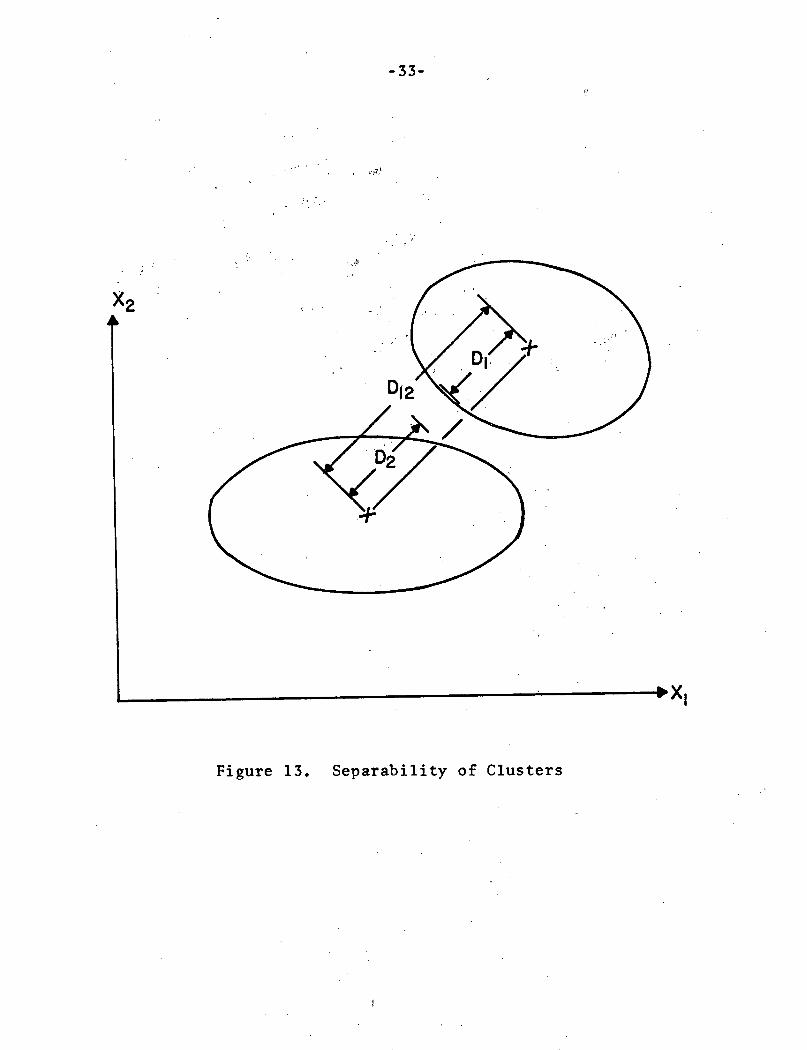
Consider two clusters and their respective ellipsoids of

concentration as shown in Figure 13. D1 2 is the distance between

the cluster centers. D1 is the distance from the center of

cluster 1 to the surface of its ellipsoid of concentration along

the line connecting the cluster centers. Similarly D2 is the

distance from the center of cluster 2 to the surface of its

ellipsoid of concentration along the line connecting the cluster

centers. In terms of these distances, D1 , D2, D1 2 , the Swain-Fu

distance is given byA A1- (54)

In terms of the cluster centers (cluster means) and the covariance

matrices associated with the clusters, the Swain-Fu distance can

be expressed as'Cc1 C2

^ = ~~~~~~~~~~(55)

Y' I+ /C Vc2

where

ck = tr{Ek (U1-U 2 )(U2-U 2 )T}

tr{A1 = trace of matrix AE

k= covariance matrix for cluster k

Uk

= mean vector for cluster k.

-33-

X24

Separability of ClustersFigure 13.

I

-34-

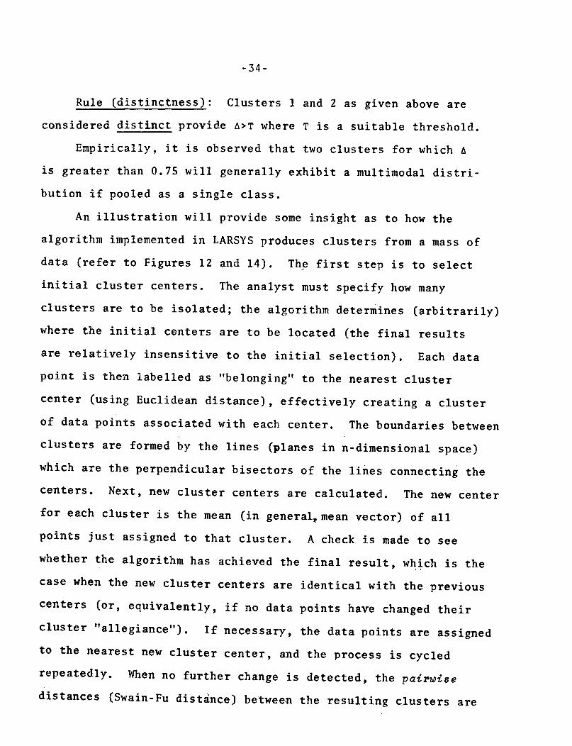
Rule (distinctness): Clusters 1 and 2 as given above are

considered distinct provide A>T where T is a suitable threshold.

Empirically, it is observed that two clusters for which A

is greater than 0.75 will generally exhibit a multimodal distri-

bution if pooled as a single class.

An illustration will provide some insight as to how the

algorithm implemented in LARSYS produces clusters from a mass of

data (refer to Figures 12 and 14). The first step is to select

initial cluster centers. The analyst must specify how many

clusters are to be isolated; the algorithm determines (arbitrarily)

where the initial centers are to be located (the final results

are relatively insensitive to the initial selection). Each data

point is then labelled as "belonging" to the nearest cluster

center (using Euclidean distance), effectively creating a cluster

of data points associated with each center. The boundaries between

clusters are formed by the lines (planes in n-dimensional space)

which are the perpendicular bisectors of the lines connecting the

centers. Next, new cluster centers are calculated. The new center

for each cluster is the mean (in general,mean vector) of all

points just assigned to that cluster. A check is made to see

whether the algorithm has achieved the final result, which is the

case when the new cluster centers are identical with the previous

centers (or, equivalently, if no data points have changed their

cluster "allegiance"). If necessary, the data points are assigned

to the nearest new cluster center, and the process is cycled

repeatedly. When no further change is detected, the pairwise

distances (Swain-Fu distance) between the resulting clusters are

-35-

cluster centersX2

X1

(a)

X2

Xl(c)

X2

(b)

X 2

(d)

Figure 14. A Sequence of Clustering Iterations(a) Initial Cluster Centers (b) (c)Intermediate Steps (d) Final CenterConfiguration.

' XI,

XII

-36-

computed and all results are printed for evaluation by the

analyst. These results include maps showing the final cluster

assignments of all points in the area(s) analyzed, and all

pairwise distances between clusters. The analyst must decide

which of the resulting clusters are distinct and which should be

pooled to define the classes for the maximum likelihood pattern

recognition analysis.

SAMPLE CLASSIFICATION

Sample classification is a slight generalization of a concept

which has been referred to in agricultural contexts as "per-field

classification." In per-field classification, a statistical

characterization of the data points in a field (actually, any

rectangular area on the ground) is calculated and compared

against the statistical characterizations of the pattern classes.

Then the field (i.e., the aggregate of points in the field) is

classified as a single unit. This is in contrast to the point-

by-point classification method discussed previously in which each

observation is given a classification which is assigned inde-

pendently of all other observations. In sample classification an

aggregate of data points is characterized and classified as in

per-field classification except that the data points need not

necessarily be taken from a spatially contiguous area (i.e., need

not comprise a field). The only requirement is that the data

points must all be assumed to be from the same class -- thus

comprising a sample from a single population, in statistical terms.

The sample classification approach has some significant

-37-

potential advantages over the more conventional point classification.

Essentially, the decision process has at hand more information on

which to base each classification decision, since it utilizes more

than a single observation. The sample classification algorithm

in LARSYS computes the sample mean and the sample covariance

matrix for the data to be classified. The averaging process tends

to eliminate the effects of system noise and other irrelevant

variability in the data. The sample covariance matrix together

with the class covariance matrices serve on one hand to provide

appropriate factors for weighting the difference between the sample

mean and each class mean; on the other hand, they may contain

information which is important in itself for characterizing the

pattern classes of interest and associating the sample with the

appropriate class. An example of the latter phenomenon has been

observed in analyzing flightlines containing both corn fields

and forested areas. The average reflectance of the forest may

be very much like the average reflectance of corn -- in fact,

single observations from each may be very nearly identical.

However, the spectral variability of forest cover is typically

much greater than that of corn and this is reflected in the

covariance matrices. As a result, the sample classifier can per-

form much more accurately than the point classifier in discrimin-

ating between corn and forest.

It should be clear to the reader from the preceding example

that the sample classification approach is more powerful than an

approach which would classify all points on an individual basis

and then classify "fields" according to "majority rules."

-38-

Formally, the sample classification procedure may be

defined as follows:

Let d(,-) be a measure defining the distance between

two probability density functions and let {p(Xlwi),

i = 1, 2, ..., m} be a set of probability density func-

tions corresponding to the classes wl, (2,....'m. If

{X} is a sample (a set of observations) with estimated

probability density p(Xlwx) then:

Decide {X} e wi if and only if

d[p p(X[x), p(X[wi)]< d[p(Xlwx), p(Xlw )]

for all i, j, = 1, 2, ..., m.

The concept of distance between probability density functions

is the same as that discussed earlier with respect to feature

selection. In fact, the same distance measure could be used,

although a different distance measure, called Jeffries-Matusita

distance (see Wacker and Landgrebe, 1971) has been implemented

in LARSYS.

For writing the definition of Jeffries-Matusita distance

(JM distance),it is convenient to use an abbreviated notation

for the density functions. Let

Pi(X) = p (Xlwi).

Then the JM distance between density functions pl(X) and p2(X)

is given by

d[pl(X),p2 (X)] [ f(/ TXp - rp27)I)2 dX]V2 (56)

where the integral is over the entire multi-dimensional space of

X. By defining

-39-

P(P1, P2) = pVTTp * Zrp-T2T dX (57)X

the JM distance can be expressed as

d[p1 (X), p2 (X)] = [2 (1-p(pl, p2))]/2. (58)

In the case of gaussian distributions with class mean vectors

Ui, covariance matrices Ei, and a sample with mean Ux and covariance

matrix Ex' Eq. (58) can be written in the form

-1 -1 1 /

(Px'Pi) * xi i (59)

12(E + Ei)11/2 ' '

Fl1 - 1 -1 -- 1 -+ z )T[ -1 -1exp - . + E U.exp ) (x Ux + i Ui)] [x Ux 1 i

+ uT 1U + Ti-1U}]U~~~ Z U i .x xx 1 i

It is significant that this expression can be evaluated without

performing explicit integration.

In practice the U's and V's are usually not known, and

estimates are used which are obtained from training patterns and

from the sample to be classified.

CONCLUDING REMARKS

The foregoing is a description of the theoretical foundations

of LARSYS, an approach to multispectral data analysis through

pattern recognition and related computer-oriented techniques.

The state-of-the-art of machine-assisted remote sensing data

analysis is changing rapidly as more powerful methods are sought

-40-

to meet ever-more-challenging remote sensing problems. It may

be expected, however, that unless some radically different approach

is developed which proves more effective, the techniques treated

herein will continue to be extensively applied. The reader who

can take time to develop a working understanding of this material

will be well equipped to apply pattern recognition techniques

to remote sensing data and to interpret with insight the analysis

results he obtains.

-ql-

References

Hall, G. H., "Data Analysis in the Social Sciences: What Aboutthe Details," Proc. Fall Joint Computer Conference, Decem-ber, 1965.

Kullback, S., Information Theory and Statistics, Wiley, NewYork, 1959.

Nilsson, N. J., Learning Machines, McGraw-Hill, 1965.

Ready, P. J., P. A. Wintz, and D. A. Landgrebe, "A LinearTransformation for Data Compression and Feature Selectionin Multispectral Imagery," LARS Information Note 072071,Laboratory for Applications of Remote-Sensing, PurdueUniversity, W. Lafayette, Indiana 47907, February 1971.

Swain, P. H., T. V. Robertson, and A. G. Wacker, "Comparison ofthe Divergence and B-Distance in Feature Selection,", LARSInformation Note 020871, Laboratory for Applications ofRemote Sensing, Purdue University, W. Lafayette, Indiana47907, February, 1971.

Wacker, A. G. and D. A. Landgrebe, "Minimum Distance Classifi-cation in Remote Sensing," LARS Information Note 030772,Laboratory for Applications of Remote Sensing, PurdueUniversity, W. Lafayette, Indiana 47907, February, 1972.