influent constituent characteristics of the modern waste stream from single sources
TRANSCRIPT

Co-published by
Influent Constituent Characteristics of theModern Waste Stream from Single Sources
Decentralized Systems
04-DEC-1.qxd 9/14/09 1:50 PM Page 1 (2,1)

04-DEC-01
INFLUENT CONSTITUENT
CHARACTERISTICS OF THE MODERN WASTE STREAM FROM SINGLE SOURCES
by: Kathryn S. Lowe
Maria B. Tucholke Jill M.B. Tomaras
Kathleen Conn Christiane Hoppe
Dr. Jörg E. Drewes Dr. John E. McCray
Dr. Junko Munakata-Marr Colorado School of Mines
Environmental Science and Engineering Division
2009
ii
For more information, contact: Water Environment Research Foundation 635 Slaters Lane, Suite 300 Alexandria, VA 22314-1177 Tel: (703) 684-2470 Fax: (703) 299-0742 www.werf.org [email protected] This report was co-published by the following organizations. For non-subscriber sales information, contact: IWA Publishing Alliance House, 12 Caxton Street London SW1H 0QS, United Kingdom Tel: +44 (0) 20 7654 5500 Fax: +44 (0) 20 7654 5555 www.iwapublishing.com [email protected] © Copyright 2009 by the Water Environment Research Foundation. All rights reserved. Permission to copy must be obtained from the Water Environment Research Foundation. Library of Congress Catalog Card Number: 2008940714 Printed in the United States of America IWAP ISBN: 978-1-84339-351-1/1-84339-351-4 This report was prepared by the organization(s) named below as an account of work sponsored by the Water Environment Research Foundation (WERF). Neither WERF, members of WERF, the organization(s) named below, nor any person acting on their behalf: (a) makes any warranty, express or implied, with respect to the use of any information, apparatus, method, or process disclosed in this report or that such use may not infringe on privately owned rights; or (b) assumes any liabilities with respect to the use of, or for damages resulting from the use of, any information, apparatus, method, or process disclosed in this report. Colorado School of Mines The research on which this report is based was developed, in part, by the United States Environmental Protection Agency (EPA) through Cooperative Agreement No. X-830851 with the Water Environment Research Foundation (WERF). However, the views expressed in this document are solely those of Colorado School of Mines and neither EPA nor WERF endorses any products or commercial services mentioned in this publication. This report is a publication of WERF, not EPA. Funds awarded under the Cooperative Agreement cited above were not used for editorial services, reproduction, printing, or distribution. This document was reviewed by a panel of independent experts selected by WERF. Mention of trade names or commercial products does not constitute WERF nor EPA endorsement or recommendations for use. Similarly, omission of products or trade names indicates nothing concerning WERF's or EPA's positions regarding product effectiveness or applicability.
The Water Environment Research Foundation, a not-for-profit organization, funds and manages water quality research for its subscribers through a diverse public-private partnership between municipal utilities, corporations, academia, industry, and the federal government. WERF subscribers include municipal and regional water and wastewater utilities, industrial corporations, environmental engineering firms, and others that share a commitment to cost-effective water quality solutions. WERF is dedicated to advancing science and technology addressing water quality issues as they impact water resources, the atmosphere, the lands, and quality of life.

Influent Constituent Characteristics of the Modern Waste Stream from Single Sources iii
This research was funded by the Water Environment Research Foundation.
Research Team Principal Investigator: Kathryn Lowe Colorado School of Mines
Co-Principal Investigators: Jörg Drewes, Ph.D. John McCray, Ph.D. Junko Munakata-Marr, Ph.D. Colorado School of Mines
Project Team: Kathleen Conn Christiane Hoppe Mike Plampin Sarah Roberts Jill Tomaras Maria Tucholke Colorado School of Mines Sara Christopherson Jessica Wittwer University of Minnesota
Tim Haeg Watab, Inc.
Harmon Harden Water Resource Consultants, LLC
WERF Project Subcommittee Damann Anderson, P.E. Hazen and Sawyer
Matt Byers, Ph.D. Zoeller Company
Edward Clerico, P.E.
ACKNOWLEDGMENTS

iv
Bob Freeman, P.E. U.S. Environmental Protection Agency
Anish Jantrania, Ph.D. Formerly with Virginia Department of Health
Charles McEntyre, P.E. Tennessee Valley Authority
Barbara Rich Deschutes County Environmental Health Division
Water Environment Research Foundation Staff Director of Research: Daniel M. Woltering, Ph.D. Senior Program Director: Amit Pramanik, Ph.D., BCEEM

Influent Constituent Characteristics of the Modern Waste Stream from Single Sources v
Abstract:
This research project characterized the composition of modern single residential source onsite raw wastewater and primary treated effluent (i.e., septic tank effluent, STE) to aid onsite wastewater system (OWS) design and management. An extensive literature review was conducted to assess the current status of knowledge related to the composition of single source raw wastewater, identify key parameters affecting wastewater composition, and identify information gaps in the current knowledge (published previously as 04-DEC-1a). This information was supplemented by a field monitoring program to assess the composition of residential OWS raw wastewater and STE. Field investigations included quarterly monitoring (fall, winter, spring, and summer) at a total of 17 sites from three regions (Colorado, Florida, and Minnesota) within the U.S. to ensure that the results and information gained had broad applicability to the management and design of OWS. A tiered monitoring approach focused on conventional constituents, microbial constituents, and organic chemicals. In addition, daily and weekly variability within the raw wastewater and STE were monitored. Information obtained was tabulated and graphically displayed to enable assessment and comparison of parameters that affect single source waste stream composition. This report describes the work performed and the findings of the second phase field monitoring.
Benefits:
♦ Comprehensive field monitoring program provides an understanding of modern raw wastewater and STE composition from single residential sources.
♦ Presents the variations in weekly and daily raw wastewater and STE composition from single residential sources due to types of indoor water use.
♦ Presents cumulative frequency distributions to enable users to assess raw wastewater and STE constituent concentrations and mass loadings to a treatment unit or the environment.
♦ Presents data in various formats (by regional location, by age of occupants, in statistical tables, and compared to literature values) to allow data users to select representative constituent values with an understanding of data limitations and potential uncertainty.
Keywords: Onsite wastewater design, onsite wastewater treatment, raw wastewater, single sources, wastewater composition.
ABSTRACT AND BENEFITS
vi
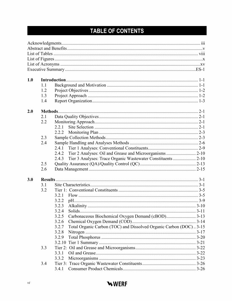
Acknowledgments.......................................................................................................................... iii Abstract and Benefits .......................................................................................................................v List of Tables ............................................................................................................................... viii List of Figures ..................................................................................................................................x List of Acronyms ...........................................................................................................................xv Executive Summary ...................................................................................................................ES-1 1.0 Introduction .................................................................................................................... 1-1 1.1 Background and Motivation ................................................................................ 1-1 1.2 Project Objectives ................................................................................................ 1-2 1.3 Project Approach ................................................................................................. 1-2 1.4 Report Organization ............................................................................................. 1-3 2.0 Methods ........................................................................................................................... 2-1 2.1 Data Quality Objectives ....................................................................................... 2-1 2.2 Monitoring Approach........................................................................................... 2-1 2.2.1 Site Selection ........................................................................................... 2-1 2.2.2 Monitoring Plan ....................................................................................... 2-3 2.3 Sample Collection Methods ................................................................................. 2-3 2.4 Sample Handling and Analyses Methods ............................................................ 2-6 2.4.1 Tier 1 Analyses: Conventional Constituents............................................ 2-9 2.4.2 Tier 2 Analyses: Oil and Grease and Microorganisms .......................... 2-10 2.4.3 Tier 3 Analyses: Trace Organic Wastewater Constituents .................... 2-10 2.5 Quality Assurance (QA)/Quality Control (QC) ................................................. 2-13 2.6 Data Management .............................................................................................. 2-15 3.0 Results ............................................................................................................................. 3-1 3.1 Site Characteristics............................................................................................... 3-1 3.2 Tier 1: Conventional Constituents ...................................................................... 3-5 3.2.1 Flow ......................................................................................................... 3-5 3.2.2 pH ............................................................................................................. 3-9 3.2.3 Alkalinity ............................................................................................... 3-10 3.2.4 Solids...................................................................................................... 3-11 3.2.5 Carbonaceous Biochemical Oxygen Demand (cBOD) .......................... 3-13 3.2.6 Chemical Oxygen Demand (COD) ........................................................ 3-14 3.2.7 Total Organic Carbon (TOC) and Dissolved Organic Carbon (DOC) .. 3-15 3.2.8 Nitrogen ................................................................................................. 3-17 3.2.9 Total Phosphorus ................................................................................... 3-20 3.2.10 Tier 1 Summary ..................................................................................... 3-21 3.3 Tier 2: Oil and Grease and Microorganisms ..................................................... 3-22 3.3.1 Oil and Grease........................................................................................ 3-22 3.3.2 Microorganisms ..................................................................................... 3-23 3.4 Tier 3: Trace Organic Wastewater Constituents ............................................... 3-26 3.4.1 Consumer Product Chemicals ................................................................ 3-26
TABLE OF CONTENTS
Influent Constituent Characteristics of the Modern Waste Stream from Single Sources vii
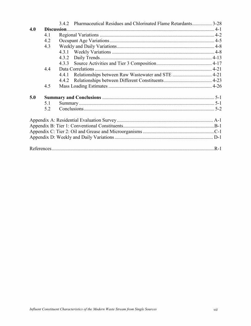
3.4.2 Pharmaceutical Residues and Chlorinated Flame Retardants ................ 3-28 4.0 Discussion........................................................................................................................ 4-1 4.1 Regional Variations ............................................................................................. 4-2 4.2 Occupant Age Variations ..................................................................................... 4-5 4.3 Weekly and Daily Variations ............................................................................... 4-8 4.3.1 Weekly Variations ................................................................................... 4-8 4.3.2 Daily Trends........................................................................................... 4-13 4.3.3 Source Activities and Tier 3 Composition ............................................. 4-17 4.4 Data Correlations ............................................................................................... 4-21 4.4.1 Relationships between Raw Wastewater and STE ................................ 4-21 4.4.2 Relationships between Different Constituents ....................................... 4-23 4.5 Mass Loading Estimates .................................................................................... 4-26 5.0 Summary and Conclusions ........................................................................................... 5-1 5.1 Summary .............................................................................................................. 5-1 5.2 Conclusions .......................................................................................................... 5-2 Appendix A: Residential Evaluation Survey .............................................................................. A-1 Appendix B: Tier 1: Conventional Constituents ..........................................................................B-1 Appendix C: Tier 2: Oil and Grease and Microorganisms ..........................................................C-1 Appendix D: Weekly and Daily Variations ................................................................................ D-1 References ....................................................................................................................................R-1

viii
2-1 Monitoring Framework ................................................................................................... 2-3 2-2 Number of Samples Collected Each Season from Each Region...................................... 2-6 2-3 Sample Analyses Methods ............................................................................................... 2-8 2-4 Sample Analyses Requirements ....................................................................................... 2-9 2-5 Summary of QC Samples Collected and Analyses Conducted ..................................... 2-13 3-1 Demographics of Residential Sites Selected for Monitoring ........................................... 3-1 3-2 Characteristics of Residential Sites Selected for Monitoring .......................................... 3-2 3-3 Selected Household Source Water Tier 1 Characteristics and Anions ............................ 3-4 3-4 Selected Cations Present in the Household Source Water (mg/L) .................................. 3-5 3-5 Estimated Septic Tank Hydraulic Residence Times at Each Site .................................... 3-7 3-6 Summary of Regional Water Use (Average Number of Events/capita/d) ...................... 3-8 3-7 Summary of Tier 1 Constituents from This Study and
Previously Reported (in mg/L) ...................................................................................... 3-22 3-8 Summary of Consumer Product Chemical Results in Raw Wastewater
from This Study ............................................................................................................. 3-26 3-9 Summary of Consumer Product Chemical Results in STE from This Study ................ 3-27 3-10 Comparison of Consumer Product Levels in Raw Wastewater and STE
in This Study to Previously Reported Levels in Residential STE and Municipal Wastewater (μg/L) ......................................................................................................... 3-27
3-11 Summary of Pharmaceutical Residues, Pesticides, and Chlorinated Flame Retardant Results in Raw Wastewater from This Study ................................................ 3-29
3-12 Summary of Pharmaceutical Residues, Pesticides, and Chlorinated Flame Retardant Results in STE from This Study .................................................................... 3-29
3-13 Comparison of Pharmaceutical Residue Levels in Raw Wastewater and STE in This Study to Previously Reported Levels in Residential STE and Municipal Wastewater (μg/L) ......................................................................................................... 3-31
4-1 ANOVA Statistics for Regional Variations of Tier 1 and Tier 2 Constituents in Raw Wastewater ......................................................................................................... 4-3
4-2 ANOVA Statistics for Regional Variations for Tier 1 and Tier 2 Constituents in STE .............................................................................................................................. 4-3
4-3 ANOVA Statistics for Occupant Age Variations of Tier 1 and Tier 2 Constituents in Raw Wastewater .......................................................................................................... 4-6
4-4 ANOVA Statistics for Occupant Age Variations of Tier 1 and Tier 2 Constituents in STE .............................................................................................................................. 4-6
4-5 Ratio of Average Concentrations of Households with Occupants >65 to Households with Occupants <65 ..................................................................................... 4-8
4-6 Summary of Water Use During Daily Trend Monitoring at Six Sites ........................... 4-13 4-7 Number of Specific Water Use Event per Capita per Time Period ............................... 4-14 4-8 Reported Pharmaceutical Use at the Field Sites ............................................................ 4-20 4-9 Summary of Mass Loading Rates of Raw Wastewater into the Septic Tank (g/capita/d) ..... 4-29 4-10 Summary of Mass Loading Rates of STE out of the Septic Tank (g/capita/d) .............. 4-29
LIST OF TABLES

Influent Constituent Characteristics of the Modern Waste Stream from Single Sources ix
B-1 Descriptive Statistics for Water Use ...............................................................................B-2 B-2 Descriptive Statistics for pH in Raw Wastewater ............................................................B-6 B-3 Descriptive Statistics for pH in STE ................................................................................B-6 B-4 Descriptive Statistics for Alkalinity in Raw Wastewater ..............................................B-10 B-5 Descriptive Statistics for Alkalinity in STE ..................................................................B-10 B-6 Descriptive Statistics for TS in Raw Wastewater ..........................................................B-14 B-7 Descriptive Statistics for TS in STE .............................................................................B-14 B-8 Descriptive Statistics for TSS in Raw Wastewater ........................................................B-18 B-9 Descriptive Statistics for TSS in STE ...........................................................................B-18 B-10 Descriptive Statistics for cBOD5 in Raw Wastewater ...................................................B-22 B-11 Descriptive Statistics for cBOD5 in STE .......................................................................B-22 B-12 Descriptive Statistics for COD in Raw Wastewater ......................................................B-27 B-13 Descriptive Statistics for COD in STE ..........................................................................B-27 B-14 Descriptive Statistics for TOC in Raw Wastewater .......................................................B-32 B-15 Descriptive Statistics for TOC in STE ...........................................................................B-32 B-16 Descriptive Statistics for DOC in Raw Wastewater ......................................................B-33 B-17 Descriptive Statistics for DOC in STE ..........................................................................B-33 B-18 Descriptive Statistics for Total Nitrogen in Raw Wastewater .......................................B-37 B-19 Descriptive Statistics for Total Nitrogen in STE ..........................................................B-37 B-20 Descriptive Statistics for Ammonium-nitrogen in Raw Wastewater .............................B-42 B-21 Descriptive Statistics for Ammonium-nitrogen in STE .................................................B-42 B-22 Descriptive Statistics for Nitrate-nitrogen in Raw Wastewater .....................................B-47 B-23 Descriptive Statistics for Nitrate-nitrogen in STE ........................................................B-47 B-24 Descriptive Statistics for Total Phosphorus in Raw Wastewater...................................B-52 B-25 Descriptive Statistics for Total Phosphorus in STE .......................................................B-52 C-1 Descriptive Statistics for Oil and Grease in Raw Wastewater .........................................C-3 C-2 Descriptive Statistics for Oil and Grease in STE .............................................................C-3 C-3 Descriptive Statistics for Fecal Coliforms in Raw Wastewater .......................................C-7 C-4 Descriptive Statistics for Fecal Coliforms in STE ...........................................................C-7 C-5 Descriptive Statistics for E. coli in Raw Wastewater ......................................................C-9 C-6 Descriptive Statistics for E. coli in STE ..........................................................................C-9 D-1 Specific Water Use during the Course of the Week at Site C-5 ..................................... D-2 D-2 Specific Water Use during the Course of the Week at Site F-2...................................... D-2 D-3 Specific Water Use during the Course of the Week at Site M-2 .................................... D-2
x
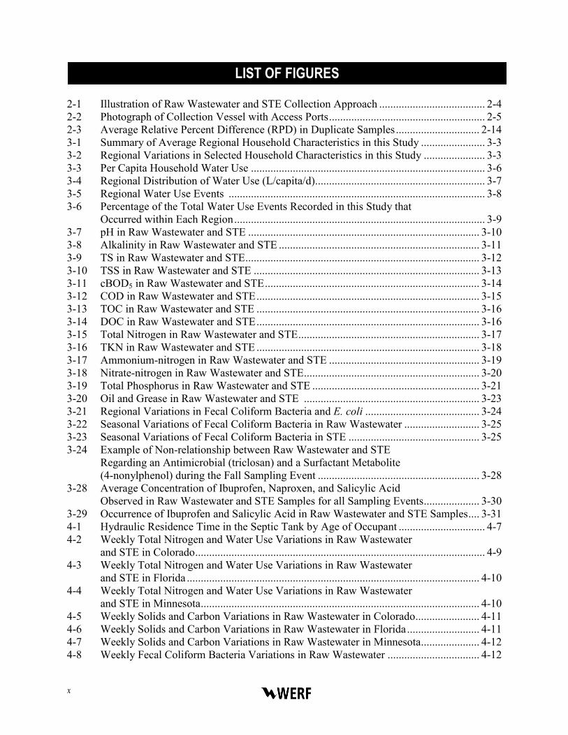
2-1 Illustration of Raw Wastewater and STE Collection Approach ...................................... 2-4 2-2 Photograph of Collection Vessel with Access Ports ........................................................ 2-5 2-3 Average Relative Percent Difference (RPD) in Duplicate Samples .............................. 2-14 3-1 Summary of Average Regional Household Characteristics in this Study ....................... 3-3 3-2 Regional Variations in Selected Household Characteristics in this Study ...................... 3-3 3-3 Per Capita Household Water Use .................................................................................... 3-6 3-4 Regional Distribution of Water Use (L/capita/d)............................................................. 3-7 3-5 Regional Water Use Events ............................................................................................ 3-8 3-6 Percentage of the Total Water Use Events Recorded in this Study that
Occurred within Each Region .......................................................................................... 3-9 3-7 pH in Raw Wastewater and STE ................................................................................... 3-10 3-8 Alkalinity in Raw Wastewater and STE ........................................................................ 3-11 3-9 TS in Raw Wastewater and STE .................................................................................... 3-12 3-10 TSS in Raw Wastewater and STE ................................................................................. 3-13 3-11 cBOD5 in Raw Wastewater and STE ............................................................................. 3-14 3-12 COD in Raw Wastewater and STE ................................................................................ 3-15 3-13 TOC in Raw Wastewater and STE ................................................................................ 3-16 3-14 DOC in Raw Wastewater and STE ................................................................................ 3-16 3-15 Total Nitrogen in Raw Wastewater and STE ................................................................. 3-17 3-16 TKN in Raw Wastewater and STE ................................................................................ 3-18 3-17 Ammonium-nitrogen in Raw Wastewater and STE ...................................................... 3-19 3-18 Nitrate-nitrogen in Raw Wastewater and STE ............................................................... 3-20 3-19 Total Phosphorus in Raw Wastewater and STE ............................................................ 3-21 3-20 Oil and Grease in Raw Wastewater and STE ............................................................... 3-23 3-21 Regional Variations in Fecal Coliform Bacteria and E. coli ......................................... 3-24 3-22 Seasonal Variations of Fecal Coliform Bacteria in Raw Wastewater ........................... 3-25 3-23 Seasonal Variations of Fecal Coliform Bacteria in STE ............................................... 3-25 3-24 Example of Non-relationship between Raw Wastewater and STE
Regarding an Antimicrobial (triclosan) and a Surfactant Metabolite (4-nonylphenol) during the Fall Sampling Event .......................................................... 3-28
3-28 Average Concentration of Ibuprofen, Naproxen, and Salicylic Acid Observed in Raw Wastewater and STE Samples for all Sampling Events .................... 3-30
3-29 Occurrence of Ibuprofen and Salicylic Acid in Raw Wastewater and STE Samples .... 3-31 4-1 Hydraulic Residence Time in the Septic Tank by Age of Occupant ............................... 4-7 4-2 Weekly Total Nitrogen and Water Use Variations in Raw Wastewater
and STE in Colorado ........................................................................................................ 4-9 4-3 Weekly Total Nitrogen and Water Use Variations in Raw Wastewater
and STE in Florida ......................................................................................................... 4-10 4-4 Weekly Total Nitrogen and Water Use Variations in Raw Wastewater
and STE in Minnesota .................................................................................................... 4-10 4-5 Weekly Solids and Carbon Variations in Raw Wastewater in Colorado ....................... 4-11 4-6 Weekly Solids and Carbon Variations in Raw Wastewater in Florida .......................... 4-11 4-7 Weekly Solids and Carbon Variations in Raw Wastewater in Minnesota ..................... 4-12 4-8 Weekly Fecal Coliform Bacteria Variations in Raw Wastewater ................................. 4-12
LIST OF FIGURES
Influent Constituent Characteristics of the Modern Waste Stream from Single Sources xi
4-9 Weekly Fecal Coliform Bacteria Variations in STE ...................................................... 4-13 4-10 Average Frequency of Water Use Events During Each Daily Trend Sample Period ... 4-15 4-11 Water Use Events Conducted During Daily Trend Sample Periods.............................. 4-15 4-12 Variation in cBOD5 Concentrations During Daily Trend Sampling ............................. 4-16 4-13 Household Activities Conducted During Daily Trend Sampling .................................. 4-16 4-14 Comparison of Triclosan-consuming Events and Raw Wastewater Concentrations
during the 24-hour Fall Sampling Event ........................................................................ 4-17 4-15 Comparison of EDTA-Consuming Events and Raw Wastewater Concentrations
during the 24-hour Fall Sampling Event ........................................................................ 4-18 4-16 Comparison of Nonylphenol-consuming Events and Raw Wastewater Concentrations during the 24-hour Fall Sampling Event ........................................................................ 4-19 4-17 Correlation between Alkalinity in Raw Wastewater and STE....................................... 4-22 4-18 Correlation between Total Phosphorus in Raw Wastewater and STE ........................... 4-22 4-19 Correlation between cBOD5 in Raw Wastewater and STE ........................................... 4-23 4-20 Correlations between TOC and DOC in Raw Wastewater and STE ............................. 4-24 4-21 Correlation between TOC and DOC in Raw Wastewater and STE Combined ............. 4-24 4-22 Correlation between cBOD5 and COD in Raw Wastewater and STE Combined ......... 4-25 4-23 Correlation between Alkalinity and Ammonium-nitrogen in Raw
Wastewater and STE ...................................................................................................... 4-26 4-24 Mass Loading Rates for cBOD5 ..................................................................................... 4-27 4-25 Mass Loading Rates for COD ........................................................................................ 4-27 4-26 Mass Loading Rates for Total Nitrogen......................................................................... 4-28 4-27 Mass Loading Rates for Total Phosphorus .................................................................... 4-29 4-28 Average Mass Loading Rates for cBOD5 and COD by Region .................................... 4-30 4-29 Average Mass Loading Rates for Nutrients by Region ................................................. 4-30 4-30 Mass Loading Rates of Raw Wastewater into the Septic Tank
for cBOD5 by Age of Occupant ..................................................................................... 4-31 4-31 Mass Loading Rates of STE Out of the Septic Tank for cBOD5 by Age of Occupant ....... 4-32 4-32 Correlation between cBOD5 Mass Loading Rates of Raw Wastewater
into the Septic Tank and of STE out of the Septic Tank .............................................. 4-33 4-33 Correlation between COD Mass Loading Rates of Raw Wastewater
into the Septic Tank and of STE out of the Septic Tank ............................................... 4-34 4-34 Correlation between Total Nitrogen Mass Loading Rates of Raw Wastewater
Into the Septic Tank and of STE Out of the Septic Tank .............................................. 4-34 4-35 Correlation between Total Phosphorus Mass Loading Rates of Raw Wastewater
Into the Septic Tank and of STE Out of the Septic Tank .............................................. 4-35 4-36 Correlation between cBOD5 and COD Mass Loading Rates of Raw Wastewater
Into the Septic Tank Combined with STE Out of the Septic Tank ................................ 4-35 4-37 Correlation between Alkalinity and Ammonium-nitrogen Mass Loading Rates of Raw
Wastewater into the Septic Tank Combined with STE out of the Septic Tank ............. 4-36 B-1 Indoor Water Use .............................................................................................................B-2 B-2 Indoor Water Use by Region ...........................................................................................B-3 B-3 Indoor Water Use by Season............................................................................................B-3 B-4 Indoor Water Use by Age ................................................................................................B-4 B-5 pH in Raw Wastewater ....................................................................................................B-5 B-6 pH in STE ........................................................................................................................B-5 B-7 pH in Raw Wastewater by Region ...................................................................................B-7
xii
B-8 pH in STE by Region .......................................................................................................B-7 B-9 pH in Raw Wastewater by Age ........................................................................................B-8 B-10 pH in STE by Age ............................................................................................................B-8 B-11 Alkalinity in Raw Wastewater .........................................................................................B-9 B-12 Alkalinity in STE .............................................................................................................B-9 B-13 Alkalinity in Raw Wastewater by Region .....................................................................B-11 B-14 Alkalinity in STE by Region..........................................................................................B-11 B-15 Alkalinity in Raw Wastewater by Season ......................................................................B-12 B-16 Alkalinity in STE by Season ..........................................................................................B-12 B-17 Alkalinity in Raw Wastewater by Age ..........................................................................B-13 B-18 Alkalinity in STE by Age ..............................................................................................B-13 B-19 TS in Raw Wastewater by Region .................................................................................B-15 B-20 TS in STE by Region .....................................................................................................B-15 B-21 TS in Raw Wastewater by Age ......................................................................................B-16 B-22 TS in STE by Age ..........................................................................................................B-16 B-23 TSS in Raw Wastewater ................................................................................................B-17 B-24 TSS in STE ....................................................................................................................B-17 B-25 TSS in Raw Wastewater by Region ...............................................................................B-19 B-26 TSS in STE by Region ...................................................................................................B-19 B-27 TSS in Raw Wastewater by Age ....................................................................................B-20 B-28 TSS in STE by Age ........................................................................................................B-20 B-29 cBOD5 in Raw Wastewater ............................................................................................B-21 B-30 cBOD5 in STE ................................................................................................................B-21 B-31 cBOD5 in Raw Wastewater by Region ..........................................................................B-23 B-32 cBOD5 in STE by Region ..............................................................................................B-23 B-33 cBOD5 in Raw Wastewater by Season ..........................................................................B-24 B-34 cBOD5 in Raw Wastewater by Season ..........................................................................B-24 B-35 cBOD5 in Raw Wastewater by Age ...............................................................................B-25 B-36 cBOD5 in STE by Age ...................................................................................................B-25 B-37 COD in Raw Wastewater ...............................................................................................B-26 B-38 COD in STE ...................................................................................................................B-26 B-39 COD in Raw Wastewater by Region .............................................................................B-28 B-40 COD in STE by Region .................................................................................................B-28 B-41 COD in Raw Wastewater by Season ............................................................................B-29 B-42 COD in STE by Season..................................................................................................B-29 B-43 COD in Raw Wastewater by Age .................................................................................B-30 B-44 COD in STE by Age ......................................................................................................B-30 B-45 TOC in Raw Wastewater and STE ................................................................................B-31 B-46 DOC in Raw Wastewater and STE ................................................................................B-31 B-47 TOC in Raw Wastewater by Region ..............................................................................B-34 B-48 TOC in STE by Region .................................................................................................B-34 B-49 DOC in Raw Wastewater by Region ............................................................................B-34 B-50 DOC in STE by Region .................................................................................................B-34 B-51 TOC in Raw Wastewater by Age...................................................................................B-35 B-52 TOC in STE by Age .......................................................................................................B-35 B-53 DOC in Raw Wastewater by Age ..................................................................................B-35 B-54 DOC in STE by Age ......................................................................................................B-35 B-55 Total Nitrogen in Raw Wastewater................................................................................B-36

Influent Constituent Characteristics of the Modern Waste Stream from Single Sources xiii
B-56 Total Nitrogen in STE ....................................................................................................B-36 B-57 Total Nitrogen in Raw Wastewater by Region ..............................................................B-38 B-58 Total Nitrogen in STE by Region ..................................................................................B-38 B-59 Total Nitrogen in Raw Wastewater by Season ..............................................................B-39 B-60 Total Nitrogen in STE by Season ..................................................................................B-39 B-61 Total Nitrogen in Raw Wastewater by Age ...................................................................B-40 B-62 Total Nitrogen in STE by Age .......................................................................................B-40 B-63 Ammonium-nitrogen in Raw Wastewater .....................................................................B-41 B-64 Ammonium-nitrogen in STE ........................................................................................B-41 B-65 Ammonium-nitrogen in Raw Wastewater by Region ....................................................B-43 B-66 Ammonium-nitrogen in STE by Region .......................................................................B-43 B-67 Ammonium-nitrogen in Raw Wastewater by Season ...................................................B-44 B-68 Ammonium-nitrogen in STE by Season .......................................................................B-44 B-69 Ammonium-nitrogen in Raw Wastewater by Age.........................................................B-45 B-70 Ammonium-nitrogen in STE by Age .............................................................................B-45 B-71 Nitrate-nitrogen in Raw Wastewater .............................................................................B-46 B-72 Nitrate-nitrogen in STE..................................................................................................B-46 B-73 Nitrate-nitrogen in Raw Wastewater by Region ............................................................B-48 B-74 Nitrate-nitrogen in STE by Region ...............................................................................B-48 B-75 Nitrate-nitrogen in Raw Wastewater by Season ...........................................................B-49 B-76 Nitrate-nitrogen in STE by Season ...............................................................................B-49 B-77 Nitrate-nitrogen in Raw Wastewater by Age .................................................................B-50 B-78 Nitrate-nitrogen in STE by Age .....................................................................................B-50 B-79 Total Phosphorus in Raw Wastewater ...........................................................................B-51 B-80 Total Phosphorus in STE ...............................................................................................B-51 B-81 Total Phosphorus in Raw Wastewater by Region..........................................................B-53 B-82 Total Phosphorus in STE by Region ..............................................................................B-53 B-83 Total Phosphorus in Raw Wastewater by Season ..........................................................B-54 B-84 Total Phosphorus in STE by Season .............................................................................B-54 B-85 Total Phosphorus in Raw Wastewater by Age ..............................................................B-55 B-86 Total Phosphorus in STE by Age...................................................................................B-55 C-1 Oil and Grease in Raw Wastewater ................................................................................C-2 C-2 Oil and Grease in STE ....................................................................................................C-2 C-3 Oil and Grease in Raw Wastewater by Region ................................................................C-4 C-4 Oil and Grease in STE by Region ....................................................................................C-4 C-5 Oil and Grease in Raw Wastewater by Age.....................................................................C-5 C-6 Oil and Grease in STE by Age .........................................................................................C-5 C-7 Fecal Coliforms in Raw Wastewater ...............................................................................C-6 C-8 Fecal Coliforms in STE ...................................................................................................C-6 C-9 E. coli in Raw Wastewater and in STE ............................................................................C-8 D-1 Weekly Variation in Alkalinity for Colorado ................................................................. D-3 D-2 Weekly Variation in Alkalinity for Florida ................................................................... D-3 D-3 Weekly Variation in Alkalinity for Minnesota ............................................................... D-4 D-4 Weekly Variation in TSS for Colorado .......................................................................... D-4 D-5 Weekly Variation in TSS for Florida .............................................................................. D-5 D-6 Weekly Variation in TSS for Minnesota ........................................................................ D-5
xiv
D-7 Weekly Variation in cBOD5 for Colorado ...................................................................... D-6 D-8 Weekly Variation in cBOD5 for Florida ......................................................................... D-6 D-9 Weekly Variation in cBOD5 for Minnesota .................................................................... D-7 D-10 Weekly Variation in Total Nitrogen for Colorado .......................................................... D-7 D-11 Weekly Variation in Total Nitrogen for Florida ............................................................. D-8 D-12 Weekly Variation in Total Nitrogen for Minnesota ........................................................ D-8 D-13 Weekly Variation in Total Phosphorus for Colorado ..................................................... D-9 D-14 Weekly Variation in Total Phosphorus for Florida ......................................................... D-9 D-15 Weekly Variation in Total Phosphorus for Minnesota ................................................. D-10 D-16 Weekly Variation in Occupants over 65 (Colorado) .................................................... D-10 D-17 Weekly Variation in Occupants under 65 (Florida) ...................................................... D-11 D-18 Weekly Variation in Occupants under 65 (Minnesota) ................................................ D-11 D-19 Percent of Constituent Contributed from Various Water Use
Activities during Daily Trend Sampling (Colorado, Three Sites) ................................ D-12 D-20 Percent of Constituent Contributed from Various Water Use
Activities during Daily Trend Sampling (Minnesota, Three Sites) .............................. D-12

Influent Constituent Characteristics of the Modern Waste Stream from Single Sources xv
AHS American Housing Survey ANOVA analysis of variance BDL below detection limit BOD biochemical oxygen demand BOD5 biochemical oxygen demand, five-day test cBOD5 carbonaceous biochemical oxygen demand, five-day test CaCO3 calcium carbonate CASRN Chemical Abstracts Service Registry Number CFD cumulative frequency distribution COD chemical oxygen demand CSM Colorado School of Mines CV coefficient of variance DOC dissolved organic carbon EDTA ethylenediaminetetraacetic acid HP Hewlett Packard GC/MS gas chromatography/mass spectrometry gpf gallons per flush IQR inter-quartile-range Lpf liters per flush MPN most probable number NP1EO 4-nonylphenolmonoethoxylate NR not reported NTA nitrilotriacetic acid OWS onsite wastewater systems QA quality assurance QC quality control R2 coefficient of determination RL reporting limit RPD relative percent difference SIM selected ion monitoring SPE solid phase extraction STE septic tank effluent TCEP tris (2-chloroethyl) phosphate TCPP tris (2-chloroisopropyl) phosphate TDCPP 1,3-dichloro-2-propanol phosphate TKN total kjeldahl nitrogen TOC total organic carbon TS total solids TSS total suspended solids UMN University of Minnesota U.S. United States U.S. EPA United States Environmental Protection Agency WWTP wastewater treatment plant
LIST OF ACRONYMS

xvi

Influent Constituent Characteristics of the Modern Waste Stream from Single Sources ES-1
EXECUTIVE SUMMARY
Proper onsite wastewater system (OWS) design, installation, operation, and management are essential to ensure protection of the water quality and the public served by that water source. Conventional OWS rely on septic tanks for the primary digestion of raw wastewater followed by discharge of primary treated effluent (i.e., septic tank effluent, STE) to the subsurface soils for eventual recharge to underlying groundwater. There have been increasing uses of alternative OWS that rely on additional treatment of STE prior to discharge to the environment in sensitive areas or may eliminate use of a septic tank altogether. Waste streams to be treated by OWS have also changed in recent years due to changing lifestyles including increasing use of personal care and home cleaning products, increasing use of pharmaceutically active compounds (e.g., antibiotics), and lower water use due to water conservation efforts. In each case, understanding the raw wastewater and/or STE composition is critical for:
♦ Successful OWS design
♦ Informed management decisions
♦ Assessment of OWS performance and environmental impacts The overall goal of this research project was to characterize modern single source OWS
raw wastewater and STE composition to aid OWS system design and management. The first phase of the project conducted a thorough literature review to assess the current status of knowledge related to the composition of single source raw wastewater and can be found in Lowe et al., 2007 and the associated database (www.ndwrcdp.org/publications). The second phase of the characterized the composition of residential single source raw wastewaters and STE. This report describes the work performed and findings of the second phase field monitoring.
Field investigations were conducted quarterly at 17 sites from three regions within the United States (U.S.). Flow-weighted 24-hour composite samples were collected from the raw wastewater and STE. A tiered monitoring approach was utilized focusing on conventional constituents, microbial constituents, and organic chemicals. Households monitored during this project had OWS that were <25 years old with concrete chambered septic tanks serving households with two to six occupants ranging in age from small children to seniors (one site served an eight-unit apartment building with 18 occupants).
The results were compiled and statistical evaluations conducted to identify general trends. Further data analyses included variations attributed to regional location, season, age of occupants and household water use. Relationships were established between a constituent in raw wastewater and STE as well as between different constituents in the waste stream. Finally, mass loading rates were estimated. Graphical tools were prepared including summary tables, cumulative frequency distribution graphs, box and whisker plots, and correlations.
Based on the findings, the following conclusions were made:
♦ The median indoor water use was ~25% lower than previous studies conducted nearly 10 years ago.
♦ The range of constituent concentrations was higher for raw wastewater compared to STE.

ES-2
♦ The consumer product chemicals – caffeine, ethylenediaminetetraacetic acid (EDTA), 4-nonylphenolmonoethoxylate (NP1EO) and triclosan – and the pharmaceutical residues – ibuprofen, naproxen, and salicylic acid – were detected in raw wastewater and STE.
♦ Significant regional variations in raw wastewater and STE concentrations were observed. Significant variations in water use and concentrations due to the age of the household occupants (either over 65 or under 65) were also observed, but no significant seasonal variation was observed.
♦ Weekly and daily variations were observed in the raw wastewater attributed to the specific water use activities with little variability observed in STE concentrations.
♦ Relationships between raw wastewater and STE concentrations, and between different constituent concentrations in raw wastewater and STE combined were established. How the difference between individual systems may have effected constituent concentrations remains unclear with insufficient replicates to further evaluate concentration relationships.
♦ Mass loading rates for constituents from raw wastewater into the septic tank and from STE out of the septic tank suggest regional differences, age of occupant differences, and better relationships between raw wastewater and STE mass loading rates as well as between different constituents (R2 > 0.50).

Influent Constituent Characteristics of the Modern Waste Stream from Single Sources 1-1
CHAPTER 1.0
INTRODUCTION
1.1 Background and Motivation Decentralized wastewater management involving onsite wastewater systems (OWS) has
been recognized as a necessary and appropriate component of a sustainable wastewater infrastructure (U.S. EPA, 1997, 2002). OWS currently serve over 21% of the U.S. population and about 28% of all new residential development (AHS, 2001). Proper OWS design, installation, operation, and management are essential to ensure protection of the water quality and the public served by that water source. Assuming soils and site conditions are judged suitable, a wide variety of OWS are designed and implemented (U.S. EPA, 1997, 2002; Crites and Tchobanoglous, 1998; Siegrist, 2001). Conventional OWS rely on septic tanks for the primary digestion of raw wastewater followed by discharge of septic tank effluent (STE) to the subsurface soils for eventual recharge to underlying groundwater (Crites and Tchobanoglous, 1998; Metcalf and Eddy, 1991; U.S. EPA, 2002). However, increasing uses of alternative OWS rely on additional treatment of the STE prior to discharge to the environment in sensitive areas or may eliminate use of a septic tank altogether. In addition, waste streams to be treated by OWS have changed during recent years due to changing lifestyles including increasing use of personal care and home cleaning products and lower water use due to water conservation efforts. Thus, information on the composition of single source OWS raw wastewater is critical for:
♦ Successful OWS design to achieve desired levels of treatment prior to discharge in the environment
♦ Informed management decisions to ensure protection of public health and the environment
♦ Use of available tools, such as model simulations at the single site-scale and the watershed-scale, to assess the effect of OWS performance and water quality impact
While much research has been done to understand the composition of STE and its treatment in the soil or with engineered treatment units, limited information on raw wastewater is available. Data reported are often of different quality or type, limiting the usefulness of the information. Furthermore, scientific understanding has not been fully or clearly documented, with studies and observations published in project reports and other formats not widely available to the field or not published at all, but retained by the researcher or practitioner (Siegrist, 2001).
To address these needs, the Water Environment Research Foundation (WERF) awarded Project Number 04-DEC-1, Influent Constituent Characteristics of the Modern Waste Stream from Single Sources to the Colorado School of Mines (CSM) in April 2005. The first phase of this research project was to conduct a thorough literature review to assess the current status of knowledge related to the composition of single source raw wastewater, identify key parameters affecting wastewater composition, and identify information gaps in the current knowledge. The literature review results can be found in Lowe et al., 2007 and the associated database (www.ndwrcdp.org/publications). Based on the findings of the literature review, the second phase of the research project was initiated to characterize the composition of residential single
1-2
source raw wastewaters and STE. The work presented here describes the approach and findings from raw wastewater and STE monitoring conducted within three regional locations of the U.S.
1.2 Project Objectives The overall goal of this research project was to characterize the extent of conventional
constituents, microbial constituents, and organic wastewater contaminants in single source OWS raw wastewater and STE to aid OWS system design and management. Specific objectives included:
♦ Determine the current state of knowledge related to the characteristics of single source OWS raw wastewater and STE.
♦ Assess single source residential OWS raw wastewater and STE.
♦ Assess variations in single source residential OWS raw wastewater and STE composition.
♦ Transfer the findings to the scientific community, system designers, and decision makers. This report describes the work performed and results to meet these objectives to assess
the composition of residential OWS raw wastewater and STE.
1.3 Project Approach The first phase of the project conducted a literature review to assess the current status of
knowledge of the composition of waste streams from single source OWS (Lowe et al., 2007). No attempt was made to screen, weight, or rank the available data. However, within the database, qualifiers were used to enable sorting of the data to evaluate what effect the parameter may or may not have on the single source waste stream composition. The data were then compiled into summary tables and cumulative frequency distribution (CFD) graphs to enable review of the data in many ways to help determine key conditions potentially affecting the composition of a single source waste stream. The results from the literature review and the database provided tools for prediction of waste stream composition useful in OWS design based on the available data. The literature review results can be found in Lowe et al., 2007 and the associated database (www.ndwrcdp.org/publications).
The second phase of the project assessed the composition of residential OWS raw wastewater and STE. A comprehensive monitoring framework was designed and implemented to evaluate the variations in single source residential OWS due to operational conditions (e.g., septic tank size, daily flow) and selected demographics (e.g., geographic location, age of occupants). To enable a more focused evaluation of residential single sources, other non-residential single sources (food, medical, non-medical) and multiple residential sources (cluster systems) were not monitored. A tiered monitoring approach was utilized focusing on conventional constituents, microbial constituents, and organic chemicals. In addition, daily and weekly variability within the raw wastewater and STE were monitored. In conjunction with the monitoring, forms were completed by the homeowners recording specific water use activities in the home and the frequency of each water use activity. Field investigations included quarterly monitoring (fall, winter, spring, and summer) at a total of 17 sites from three regions within the U.S. to ensure that the results and information gained have broad applicability to the management and design of OWS.
Influent Constituent Characteristics of the Modern Waste Stream from Single Sources 1-3
1.4 Report Organization This report is organized into five chapters. The first chapter provides an introduction and
purpose for this project. Chapter 2.0 describes the methods employed during and in support of field monitoring. The results of the residential OWS raw wastewater and STE monitoring are presented in Chapter 3.0. Chapter 4.0 discusses variations within the data collected and tools for assessing and estimating raw wastewater and STE composition. The last chapter provides a summary of the project and conclusions. Statistical summaries and supporting graphs of all the data obtained are provided in appendices.

1-4

Influent Constituent Characteristics of the Modern Waste Stream from Single Sources 2-1
CHAPTER 2.0
METHODS 2.1 Data Quality Objectives
The overall data quality objective was to ensure the raw wastewater and STE data collected from residential single sources were of sufficient quality to characterize the concentration of conventional constituents, microbial constituents, and organic chemicals present in the waste stream. It is recognized that the composition of raw wastewater: 1) is highly variable (primarily due to solids), 2) does not reflect treatment achieved in the tanks used in the vast majority of OWS to equalize flow and provide settling of solids, and 3) may not reflect constituents of interest present in the waste stream such as certain trace organic constituents which undergo transformation in the septic tank prior to discharge to the environment. To overcome these issues, both the raw wastewater and STE were monitored. Specific data quality objectives were to:
♦ ensure that sites selected for monitoring were representative of the target waste stream;
♦ ensure that raw wastewater and STE samples were of sufficient quality to assess the presence and concentration of Tier 1 constituents (pH, alkalinity, carbon, solids, nutrients, fecal coliform bacteria);
♦ ensure that raw wastewater and STE samples were of sufficient quality to assess the presence and concentration of Tier 2 constituents (oil and grease, E. coli, coliphage);
♦ ensure that raw wastewater and STE samples were of sufficient quality to assess the presence and concentration of Tier 3 constituents (consumer product chemicals, pharmaceutical residues, pesticides, and chlorinated flame retardants); and
♦ ensure sufficient sample frequency to assess variability within a single source waste stream and estimate mass loading rates.
2.2 Monitoring Approach 2.2.1 Site Selection
During the Phase 1 Literature Review, the prevalence of various single source OWS currently installed and in operation were assessed (Lowe et al., 2007). Each state agency responsible for OWS regulation was contacted. Of all the responding states, only Florida, New Mexico, and North Carolina had databases useful for determining the prevalence of systems. Based on the limited state and county available data, queries of the U.S. Census were conducted. From these data sources, domestic (residential) sources were the most prevalent (at a minimum of approximately >75% of OWS within a state) systems in use.
Data from the U.S. Census Bureau (AHS, 2001) indicated that regionally, in the Northeast 21.3% of the total households were served by OWS, 19.9% in the Midwest, 26.5% in the South, and 13.0% of the total households in the West were served by OWS. Selected demographics to capture differences in lifestyle habits that could affect raw wastewater
2-2
composition were also assessed including: over the age of 65, location (urban vs. rural), new construction, poverty, and ethnicity. Three broad, but distinct regional locations, appeared to encompass the observed differences in these demographics:
♦ West ♦ South ♦ Midwest ♦ Northeast
For example, as a representative state in the south, Florida has a medium percentage of the region’s occupied households served by OWS, high annual average temperatures and precipitation, low percentage of rural systems, average levels of poverty, and high percentage of individuals over age 65. Evaluation of the literature data on waste stream composition also suggested regional variations in single residential raw wastewater and STE (Lowe et al., 2007). For example, the highest median concentrations of nutrients (nitrogen and phosphorus) were found in the West. Based on the prevalence of systems identified during Phase 1 and the possible regional influence on composition, raw wastewater and STE monitoring occurred at residential sites from three regional locations: Colorado (the west), Florida (the south), and Minnesota (the midwest and northeast). Regional liaisons with previous experience in OWS monitoring were established in Florida and Minnesota. The Florida regional liaison was Water Research Consulting, LLC. The Minnesota regional liaison was the University of Minnesota (UMN). The regional liaisons identified potential applicable sites, interfaced with the homeowners, and assisted with sample collection. A regional liaison was not identified in Colorado since project team members from CSM were located in Colorado. In each region, the selected homeowners were very interested and willing to participate in the project and provided detailed information about their water use and other relevant information (e.g. brand of detergents, soaps, medications, etc.).
Factors that were considered during site selection included age and type of system, age of occupants, depth of the wastewater line from the house to the septic tank, topography, and landscaping. In addition, a 20-amp power source and a water spigot needed to be available at each location. Although system age and other demographics, such as race or income, were not factors that were analyzed in this project, care was taken to obtain test sites that represented the general population in each state. Similar site characteristics also enabled comparison of sites between the three regions. While numerous subtleties exist between waste streams from a single residential source, the key demographics that were hypothesized to affect daily flow and/or composition were: occupancy (two vs. four occupants) and age of occupants (<65 years of age vs. >65 years of age). Higher occupancy was anticipated to increase the daily water use with variation in household contributions (toilet, laundry, bathing/showering). These differences could affect waste stream concentrations and potentially per capita mass loading rates from the septic tank to subsequent treatment units (e.g., media filters, soil treatment units, etc.). It was also hypothesized that occupants over the age of 65 could be more likely to contribute higher loads of pharmaceuticals and other trace organic wastewater contaminants (Tier 3) to the waste stream due to potential increased use of medications. These households with occupants over the age of 65 were also assumed to have fewer total occupants per household resulting in potentially lower water use.
During site selection a survey was conducted to collect pertinent information related to the household and OWS inputs at that site (Appendix A).

Influent Constituent Characteristics of the Modern Waste Stream from Single Sources 2-3
2.2.2 Monitoring Plan Residential sites were monitored to determine basic information on single source raw
wastewater as well as capture significant events of interest (e.g., laundry). A tiered approach to monitoring was used. Tier 1 parameters were monitored at all sites and included operational parameters, design parameters, and conventional constituents of interest to obtain basic information on single source OWS. Operational parameters included temperature and daily flow. Conventional constituents included pH, alkalinity, solids (total solids [TS] and total suspended solids [TSS]), organic carbon (carbonaceous biochemical oxygen demand [cBOD5], chemical oxygen demand [COD], total organic carbon [TOC], and dissolved organic carbon [DOC]), nutrients (total nitrogen, ammonium-nitrogen, nitrate-nitrogen, and total phosphorous), and fecal coliform bacteria. Design parameters including the number of tanks and the size of the tanks were initially recorded by the homeowner on the site survey and verified by the project team on the first visit to the location. Tier 2 parameters were monitored at 50% of the sites at a minimum and included oil and grease and microorganisms (E. coli and coliphage). Tier 3 included organic trace chemicals which were monitored at a total of six sites (two in each region) during three sampling events (fall, winter, and spring).
Flow-weighted 24-hour composite samples were collected from the raw wastewater and STE. To capture potential seasonal effects, sites were monitored quarterly (fall, winter, spring, and summer). At six sites (C1, C3, C5, M1, M2, and M4) monitoring was conducted at a higher frequency to capture waste stream variations attributed to specific events (e.g., toilet flushing, laundry). During this monitoring, homeowners were provided a log to record activities conducted during the sampling period. The sampling periods varied slightly due to the differing schedules of the homeowners. In addition, at three sites (C5, F2, and M2) 24-hr flow-weighted composite samples were collected for seven sequential days to assess weekly variations.
The monitoring approach is summarized in Table 2-1. Table 2-1. Monitoring Framework.
Monitoring Tier
Number of Sites
Sample Matrix
Sample Event Analyses Parameters / Constituents
Tier 1 17 Raw and STE
Fall, Winter, Spring, Summer
Flow, pH, alkalinity, TS, TSS, cBOD5, COD, TOC, DOC, total nitrogen, ammonium, nitrate, total phosphorus, fecal coliforms
Tier 2 10 Raw and STE
Fall, Winter, Spring, Summer
oil and grease (32 samples), E.Coli (all sites), coliphage
Tier 3 6 Raw and STE
Fall, Winter, Spring
4-nonylphenol, 4-t-octylphenol, nonylphenolpolyethoxylates, 4-t-octylphenolpolyethoxylates, bisphenol A, caffeine, triclosan, 1,4-dichlorobenzene, clofibric acid, dichloroprop, diclofenac, fenofibrate, gemfibrozil, ibuprofen, ketoprofen, mecoprop, naproxen, phenacetine, salicylic acid, Tris (2-chloroethyl) phosphate (TCEP), Tris (2-chloroisopropyl) phosphate (TCPP), 1,3-dichloro-2-propanol phosphate (TDCPP)
Tier 1 6 Raw During the Summer sampling event, composite samples were collected at a higher frequency to capture specific household activities
Tier 1 3 Raw and STE
During the Spring sampling event, composite samples were collected every 24 hrs for 7 days to capture weekly variations
2.3 Sample Collection Methods Flow-weighted 24-hour composite samples were collected to capture the overall extent of
constituents in the waste stream. Raw wastewater was homogenized prior to collection of raw
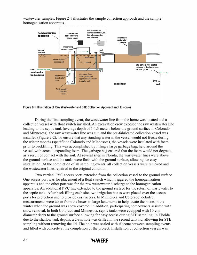
2-4
wastewater samples. Figure 2-1 illustrates the sample collection approach and the sample homogenization apparatus.
7.5-L samplecollection
vessel
septic tank
rawwastewaterfrom source float switch
to activatepump
maceratingvacuum pump
raw wastewater sample container, onice with secondarycontainment
flow meter
quick connect
ground surface
homogenizationapparatus
converter and back-up battery
power supply
observation/access port
automatedwastewater
sampler
STE sample inlet locatedjust prior to discharge from the tank (in the “T”)
ball valve
discharge from homogenization apparatus with returnto septic tank STE to
soil
Figure 2-1. Illustration of Raw Wastewater and STE Collection Approach (not to scale).
During the first sampling event, the wastewater line from the home was located and a collection vessel with float switch installed. An excavation crew exposed the raw wastewater line leading to the septic tank (average depth of 1-1.3 meters below the ground surface in Colorado and Minnesota), the raw wastewater line was cut, and the pre-fabricated collection vessel was installed (Figure 2-2). To ensure that any standing water in the vessel would not freeze during the winter months (specific to Colorado and Minnesota), the vessels were insulated with foam prior to backfilling. This was accomplished by filling a large garbage bag, held around the vessel, with aerosol expanding foam. The garbage bag ensured that the foam would not degrade as a result of contact with the soil. At several sites in Florida, the wastewater lines were above the ground surface and the tanks were flush with the ground surface, allowing for easy installation. At the completion of all sampling events, all collection vessels were removed and the wastewater lines repaired to the original condition.
Two vertical PVC access ports extended from the collection vessel to the ground surface. One access port was for placement of a float switch which triggered the homogenization apparatus and the other port was for the raw wastewater discharge to the homogenization apparatus. An additional PVC line extended to the ground surface for the return of wastewater to the septic tank. After back filling each site, two irrigation boxes were placed over the access ports for protection and to provide easy access. In Minnesota and Colorado, detailed measurements were taken from the boxes to large landmarks to help locate the boxes in the winter when the ground was snow covered. In addition, participating homeowners assisted with snow removal. In both Colorado and Minnesota, septic tanks were equipped with 10-cm diameter risers to the ground surface allowing for easy access during STE sampling. In Florida due to the shallow tank depths, a 2-cm hole was drilled in the second tank lid, allowing for STE sampling without removing the lid. The hole was sealed with silicone between sampling events and filled with concrete at the completion of the project. Installation of collection vessels was
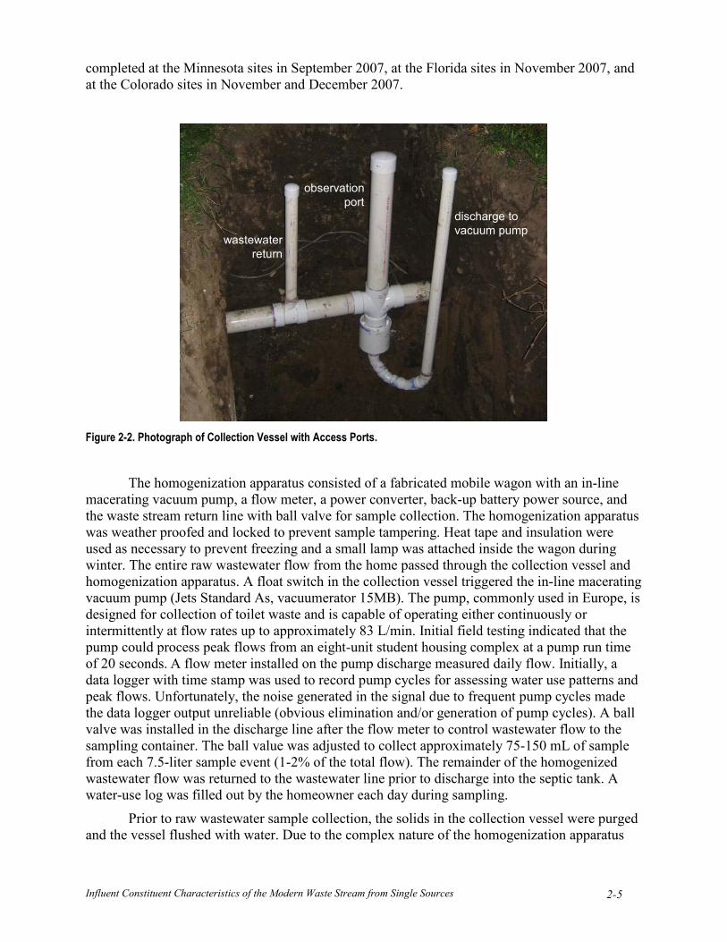
Influent Constituent Characteristics of the Modern Waste Stream from Single Sources 2-5
completed at the Minnesota sites in September 2007, at the Florida sites in November 2007, and at the Colorado sites in November and December 2007.
discharge tovacuum pump
observationport
wastewaterreturn
discharge tovacuum pump
observationport
wastewaterreturn
Figure 2-2. Photograph of Collection Vessel with Access Ports.
The homogenization apparatus consisted of a fabricated mobile wagon with an in-line macerating vacuum pump, a flow meter, a power converter, back-up battery power source, and the waste stream return line with ball valve for sample collection. The homogenization apparatus was weather proofed and locked to prevent sample tampering. Heat tape and insulation were used as necessary to prevent freezing and a small lamp was attached inside the wagon during winter. The entire raw wastewater flow from the home passed through the collection vessel and homogenization apparatus. A float switch in the collection vessel triggered the in-line macerating vacuum pump (Jets Standard As, vacuumerator 15MB). The pump, commonly used in Europe, is designed for collection of toilet waste and is capable of operating either continuously or intermittently at flow rates up to approximately 83 L/min. Initial field testing indicated that the pump could process peak flows from an eight-unit student housing complex at a pump run time of 20 seconds. A flow meter installed on the pump discharge measured daily flow. Initially, a data logger with time stamp was used to record pump cycles for assessing water use patterns and peak flows. Unfortunately, the noise generated in the signal due to frequent pump cycles made the data logger output unreliable (obvious elimination and/or generation of pump cycles). A ball valve was installed in the discharge line after the flow meter to control wastewater flow to the sampling container. The ball value was adjusted to collect approximately 75-150 mL of sample from each 7.5-liter sample event (1-2% of the total flow). The remainder of the homogenized wastewater flow was returned to the wastewater line prior to discharge into the septic tank. A water-use log was filled out by the homeowner each day during sampling.
Prior to raw wastewater sample collection, the solids in the collection vessel were purged and the vessel flushed with water. Due to the complex nature of the homogenization apparatus

2-6
(i.e., vacuum pump, flow meter, PVC connections and polyethylene tubing) and the waste stream being sampled (i.e., raw wastewater with high concentrations of the constituents being analyzed for), this system flush also served to decontaminate the homogenization apparatus between sites. Approximately 20 L of tap water was used during the flush. However, if the discharge stream from the wagon visually appeared “dirty”, additional clean water was flushed through the system. Finally, prior to sample collection, up to four exchanges of wastewater from the 7.5-L collection vessel was passed through the system.
STE samples were collected using an automated composite sampler (Isco, Inc. Wastewater Sampler, Model 3250). The suction inlet tubing from the automated sampler was located in the mid section of the clear liquid phase of the lattermost tank immediately prior to discharge to the soil treatment unit. The autosampler was programmed to collect 150 mL of STE every 30 minutes over the 24-hour sampling event.
This monitoring design resulted in a total of 68 raw wastewater and STE samples (17 sites x 4 seasons). However, due to low sample volume, homeowner vacations, and on one occasion, a failed soil treatment unit, the actual number of samples collected during this project varied (Table 2-2).
Table 2-2. Number of Samples Collected Each Season from Each Region.
Tier 1 Tier 2 Tier 3 Raw STE Raw STE Raw STE
Colorado* Fall 5 5 3 4 2 2 Winter 5 5 5 4 2 2 Spring 5 5 2 2 2 2 Summer 5 5 1 1 0 0
Florida Fall 6 6 6 6 2 2 Winter 6 6 6 6 2 2 Spring 6 6 2 2 2 2 Summer 6 6 3 3 0 0
Minnesota Fall 5 4 0 0 0 0 Winter 4 3 2 2 2 2 Spring 5 5 1 1 2 2 Summer 5 5 3 2 0 0
Total 63 61 27 27 16 16 *Excludes eight-unit multi-family location in Colorado
To assess weekly variations in the waste stream, both raw wastewater and STE 24-hr composite samples were collected every day for one week at one site in each region (at the Colorado site, STE was sampled for nine days). Both the homogenization apparatus and STE autosampler were started and the collection jars replaced at the same time each day. Daily flow was recorded and samples were analyzed for Tier 1 constituents. To assess daily variations due to specific water uses (e.g., laundry), up to five raw wastewater composite samples were collected throughout the day at six sites; three sites each in Colorado and Minnesota. STE samples were not collected due to the longer hydraulic residence times in the septic tank. For the daily variation monitoring, efforts were made to cover morning, daily, evening and overnight activities. However, sample durations varied due to homeowner schedules.
Influent Constituent Characteristics of the Modern Waste Stream from Single Sources 2-7
2.4 Sample Handling and Analyses Methods Sample handling procedures included the use of correct sample containers, labeling,
documentation, preservation, and shipment. Tables 2-3 and 2-4 list the Tier 1, Tier 2, and Tier 3 analytical methods, sample containers, preservatives, and holding times. Raw wastewater samples were collected into a 9.6 L glass jar kept on ice at 4°C in coolers. After the 24-hr sampling period, the 9.6 L sample jar was mixed and sample aliquots transferred into amber glass bottles with preservatives specific for Tier 1, 2, or 3 analyses. Field duplicate samples were collected from the same sample jar. Each sample aliquot was labeled with the Site ID, date, and sample type (i.e., raw, STE, raw-dup, or STE-dup) and logged into laboratory notebooks. Initially a six-port manifold was used to split the waste stream simultaneously into 6 different bottles; two bottles for field samples without preservative, one bottle each for oil and grease and total kjeldahl nitrogen (TKN) analyses with H2SO4 preservative, one bottle with 1% formalin preservative for Tier 3 Method 1, and one bottle with sodium azide preservative for Tier 3 Method 2). However, field testing indicated that the manifold preferentially directed sample volume to different bottles resulting in different samples in each bottle over the 24-hr composite sample. To ensure that collection of smaller samples from the composite sample would be representative of the sample, six different aliquots from the 9.6 L sample jar were collected. Results indicated less than 5% coefficient of variance (CV) within the six aliquots in Tier 1 constituents for both raw wastewater and STE (excluding nitrate-nitrogen, 15% CV in raw wastewater and 19% CV in STE). This suggested that this was a representative and preferred sample handling method.
Similar to the raw wastewater sample handling, STE was collected into a 9.6 L jar and then mixed and poured into appropriate containers for Tier 1, 2, and 3 analyses. Field duplicate samples were collected from the same sample jar.
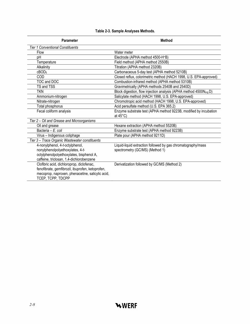
2-8
Table 2-3. Sample Analyses Methods.
Parameter Method Tier 1 Conventional Constituents
Flow Water meter pH Electrode (APHA method 4500-H+B) Temperature Field method (APHA method 2550B) Alkalinity Titration (APHA method 2320B) cBOD5 Carbonaceous 5-day test (APHA method 5210B) COD Closed reflux, colorimetric method (HACH 1998, U.S. EPA-approved) TOC and DOC Combustion-infrared method (APHA method 5310B) TS and TSS Gravimetrically (APHA methods 2540B and 2540D) TKN Block digestion, flow injection analysis (APHA method 4500Norg D) Ammonium-nitrogen Salicylate method (HACH 1998, U.S. EPA-approved) Nitrate-nitrogen Chromotropic acid method (HACH 1998, U.S. EPA-approved) Total phosphorus Acid persulfate method (U.S. EPA 365.2) Fecal coliform analysis Enzyme substrate test (APHA method 9223B, modified by incubation
at 45°C) Tier 2 – Oil and Grease and Microorganisms
Oil and grease Hexane extraction (APHA method 5520B) Bacteria – E. coli Enzyme substrate test (APHA method 9223B) Virus – Indigenous coliphage Plate pour (APHA method 9211D)
Tier 3 – Trace Organic Wastewater constituents 4-nonylphenol, 4-t-octylphenol, nonylphenolpolyethoxylates, 4-t-octylphenolpolyethoxylates, bisphenol A, caffeine, triclosan, 1,4-dichlorobenzene
Liquid-liquid extraction followed by gas chromatography/mass spectrometry (GC/MS) (Method 1)
Clofibric acid, dichloroprop, diclofenac, fenofibrate, gemfibrozil, ibuprofen, ketoprofen, mecoprop, naproxen, phenacetine, salicylic acid, TCEP, TCPP, TDCPP
Derivatization followed by GC/MS (Method 2)
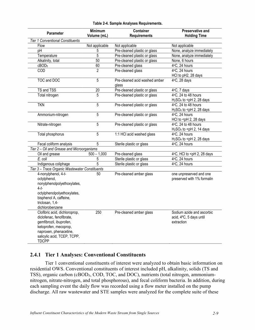
Influent Constituent Characteristics of the Modern Waste Stream from Single Sources 2-9
Table 2-4. Sample Analyses Requirements.
Parameter Minimum Volume (mL)
Container Requirements
Preservative and Holding Time
Tier 1 Conventional Constituents Flow Not applicable Not applicable Not applicable pH 5 Pre-cleaned plastic or glass None, analyze immediately Temperature 5 Pre-cleaned plastic or glass None, analyze immediately Alkalinity, total 50 Pre-cleaned plastic or glass None, 6 hours cBOD5 60 Pre-cleaned glass 4oC, 24 hours COD 2 Pre-cleaned glass 4oC, 24 hours
HCl to pH2, 28 days TOC and DOC 5 Pre-cleaned acid washed amber
glass 4oC, 28 days
TS and TSS 20 Pre-cleaned plastic or glass 4oC, 7 days Total nitrogen 5 Pre-cleaned plastic or glass 4oC, 24 to 48 hours
H2SO4 to <pH 2, 28 days TKN 5 Pre-cleaned plastic or glass 4oC, 24 to 48 hours
H2SO4 to <pH 2, 28 days Ammonium-nitrogen 5 Pre-cleaned plastic or glass 4oC, 24 hours
HCl to <pH 2, 28 days Nitrate-nitrogen 5 Pre-cleaned plastic or glass 4oC, 24 to 48 hours
H2SO4 to <pH 2, 14 days Total phosphorus 5 1:1 HCl acid washed glass 4oC, 24 hours
H2SO4 to <pH 2, 28 days Fecal coliform analysis 5 Sterile plastic or glass 4oC, 24 hours
Tier 2 – Oil and Grease and Microorganisms Oil and grease 500 – 1,000 Pre-cleaned glass 4oC, HCl to <pH 2, 28 days E. coli 5 Sterile plastic or glass 4oC, 24 hours Indigenous coliphage 5 Sterile plastic or glass 4oC, 24 hours
Tier 3 – Trace Organic Wastewater Constituents 4-nonylphenol, 4-t-octylphenol, nonylphenolpolyethoxylates, 4-t-octylphenolpolyethoxylates, bisphenol A, caffeine, triclosan, 1,4-dichlorobenzene
50 Pre-cleaned amber glass one unpreserved and one preserved with 1% formalin
Clofibric acid, dichloroprop, diclofenac, fenofibrate, gemfibrozil, ibuprofen, ketoprofen, mecoprop, naproxen, phenacetine, salicylic acid, TCEP, TCPP, TDCPP
250 Pre-cleaned amber glass Sodium azide and ascorbic acid, 4ºC, 5 days until extraction
2.4.1 Tier 1 Analyses: Conventional Constituents Tier 1 conventional constituents of interest were analyzed to obtain basic information on
residential OWS. Conventional constituents of interest included pH, alkalinity, solids (TS and TSS), organic carbon (cBOD5, COD, TOC, and DOC), nutrients (total nitrogen, ammonium-nitrogen, nitrate-nitrogen, and total phosphorous), and fecal coliform bacteria. In addition, during each sampling event the daily flow was recorded using a flow meter installed on the pump discharge. All raw wastewater and STE samples were analyzed for the complete suite of these

2-10
constituents following standard methods as described in Table 2-3 (APHA, 2005; Hach, 1998). Samples were transferred into 500 mL amber glass containers and stored at 4°C until overnight delivery to the CSM laboratory for analysis. Samples were unfiltered and analyzed within the appropriate holding times as specified in individual analysis methods (Table 2-4). Laboratory testing indicated no interference due to the presence of unfiltered solids with colorimetric analytical techniques. All sample containers were decontaminated (soap wash, triple deionized water rinse, and acid/base wash as required) between sampling locations.
2.4.2 Tier 2 Analyses: Oil and Grease and Microorganisms Tier 2 sample analyses included oil and grease and microorganisms. Raw wastewater and
STE samples were transferred into pre-cleaned glass bottles with H2SO4 preservative for oil and grease and sterile plastic containers for microorganisms. Approximately 50% of the samples collected were submitted for oil and grease analysis (from ten sites during the fall sampling event, 13 sites in winter, five sites in spring, and at seven sites during the summer sampling event). Oil and grease analysis was performed using hexane extraction (U.S. EPA method 1664) by a commercial laboratory. Microbial analyses were conduced at CSM on all of the samples (excluding coliphage which was analyzed in 20% of the samples). All samples were stored at 4°C until delivery to the CSM or commercial analytical laboratory.
Although described in this chapter because of similar analytical techniques, fecal coliforms were a Tier 1 microbial parameter. Tier 2 microbiological constituents included coliphage and E. coli. Approximately 15 mL of sample was placed into a sterilized container and immediately placed on ice. Samples were then shipped overnight shipped to CSM for quantification of coliphage numbers, fecal coliform counts, and E. coli counts. Studies have shown that sample holding times of up to 24 hours have little impact on bacterial counts or coliphage numbers (Van Cuyk, 2003; Selvakumar et al., 2004).
Coliphage detection was conducted using APHA (2005) method 9211 D. Samples were mixed with growth media and the coliphage specific host, E. coli, and then poured into petri dishes. The mixture was allowed to harden and then incubated at 37°C for up to 24 hours. The incubation plaques were counted and the coliphage concentration determined.
Both fecal coliforms (Tier 1) and E. coli (Tier 2) were enumerated using a modified version of the enzyme substrate test (APHA 2005, 9223B (Colilert®). Samples were diluted and added to a chromogenic and flourogenic substrate. After adding sample to the substrates, the mixture was incubated at 45°C for 24 hours. This method provided the concentrations of both fecal coliforms and E. coli through a most probable number (MPN) result. The incubation temperature was modified from the manufacturer’s recommendation of 35°C in order to enumerated only fecal coliforms rather than total coliforms. Several groups (Yakub et al., 2002; Chihara et al., 2005) have shown similar fecal coliform counts when comparing the above method to the membrane filtration method (APHA 2005, 9222D).
2.4.3 Tier 3 Analyses: Trace Organic Wastewater Constituents Six sites, two from each geographic region, were selected for analysis of Tier 3
constituents: C1, C3, F2, F4, M1, and M3. In each geographic region, one site served a high-occupancy household with four to five adults and children and the other site served a low-occupancy household with two to three adults or seniors. Tier 3 constituents were measured using two methods for trace organic wastewater constituents established at CSM. Method 1 quantified the consumer product chemicals 4-nonylphenol, 4-nonylphenolmonoethoxylate (NP1EO), ethylenediaminetetraacetic acid (EDTA), nitrilotriacetic acid (NTA), bisphenol A,
Influent Constituent Characteristics of the Modern Waste Stream from Single Sources 2-11
caffeine, and triclosan. Method 2 quantified pharmaceutical residues (ibuprofen, naproxen, gemfibrozil, diclofenac, salicylic acid), pesticides (mecoprop, dicloprop), and chlorinated flame retardants (tris (2-chloroethyl) phosphate [TCEP], tris (2-chloroisopropyl) phosphate [TCPP], 1,3-dichloro-2-propanol phosphate [TDCPP]). During the fall, winter, and spring sampling events, 24-hour composite samples of raw wastewater and STE were collected and were transferred into pre-cleaned amber glass bottles with preservative (Method 1: one unpreserved and one preserved with 1% formalin, v/v; Method 2: 1 g sodium azide), and stored at 4ºC until analysis, which was conducted within 72 hours of sample collection.
A spike experiment was carried out prior to field monitoring. Homogenized raw wastewater was collected with three dilutions (1, 5, and 10 mL) of the sample diluted into 250 mL of distilled water, extracted and derivatized using Methods 1 and 2. Distilled water matrix spike recoveries averaged 86% (ranging from 45-126%, n=25) while environmental sample matrix spike recoveries average 90% (ranging from 43-154%, n=22). Based on these percent recoveries of surrogate standards, the instrument sensitivity was determined for raw wastewater matrices.
Due to the difficulties with collecting split samples directly into preserved sample containers, a sample holding test was also conducted prior to field monitoring. Testing showed that preservation of the samples after the 24 hour composite event compared to during the event had little impact on the recovery of the constituents analyzed (both Methods 1 and 2). In addition, there was no evidence of loss/degradation during a 72-hour holding time for Method 1 with ≥ 85% recovery for consumer product chemicals in STE (which is within the range of analytical variability). Raw wastewater samples increased the difficulty in analysis with < 35% difference in analyte recovery between holding times of 0 hrs and 72 hrs.
2.4.3.1 Consumer Product Chemicals (Method 1) Consumer product chemicals including bisphenol A, caffeine, 4-nonylphenol, NP1EO,
and triclosan were analyzed using a solid-phase extraction (SPE) followed by analysis by electron impact gas chromatography/mass spectrometry (GC/MS). A 50 mL unpreserved, unfiltered sample was spiked with surrogate standards (d6-bisphenol A, d9-caffeine, 4-n-nonylphenol and 4-n-NP1EO) and passed through a pre-conditioned cartridge (Waters tC18+, conditioned with dichloromethane, methanol, and distilled water) at a rate of approximately 5 mL/min. Samples were often diluted 2:1 or more with distilled water to minimize matrix effects. Cartridges were rinsed with a 20% methanol/80% distilled water solution to elute interfering polar compounds. Target compounds were eluted with dichloromethane into anhydrous sodium sulfate, and passed over a sodium sulfate drying column to remove any residual water. The extract was concentrated under nitrogen gas to 0.5 mL and transferred to a GC/MS vial for analysis by capillary column GC/MS.
The metal-chelating agents EDTA and NTA required derivatization for analysis by GC/MS due to their active functional groups and nonvolatility. A 100-mL formalin-preserved sample was spiked with the surrogate standard d12-EDTA and evaporated to dryness at 90°C for 36 hours. Wastewater samples were often diluted 2:1 or more with distilled water to minimize matrix effects. After cooling, formic acid was added and the sample was rotary vacuum evaporated to dryness. The residue was reacted with 1-propanol/acetyl chloride (10% v/v) to form the propyl esters of the analytes. The analytes were extracted into chloroform and passed over a sodium sulfate drying column to remove any residual water. The chloroform was evaporated to dryness by nitrogen gas. The residue was re-dissolved in 200 µL of toluene and

2-12
spiked with 25 µL of the injection standard 1-phenylnonane. The extract was transferred to a GC/MS vial for analysis by capillary column GC/MS.
Extracts from both sample extraction methods were analyzed by electron impact GC/MS in the full scan and selected ion monitoring (SIM) modes. The general gas chromatography conditions were: Hewlett Packard (HP) 6890 GC; column – HP Ultra II (5% phenylmethyl silicone), 25 m x 0.2 mm, 33 µm film thickness; carrier gas – ultra high purity helium with a linear flow velocity of 27 cm/sec; injection port temperature – 300ºC; initial oven temperature – 140ºC (SPE), 100ºC (derivatization); split vent open – 0.75 min; ramp rate – 6ºC/minute to 300ºC; hold time – 15 minutes at 300ºC. The mass spectrometer conditions were: HP 5793 Mass Selective Detector; tune with perfluorotributylamine; ionization energy – 70 eV; source temperature – 250ºC; interface temperature 300ºC; full scan – 40 to 550 atomic mass units at 1 scan/second.
Target compound concentrations were calculated based on SIM data using diagnostic ions for each compound. Each compound was identified based on a peak signal to noise ratio of at least 3:1, matching of retention times (± 0.02 min) and ion ratios (± 20%) determined from analysis of authentic standards. A seven-point standard curve based on the response ratio to a surrogate standard was used for calculating concentrations. Distilled water, distilled water matrix spikes, and sample matrix spikes comprised approximately 20% of analyses. Each sampling location was analyzed in duplicate or triplicate (field and/or laboratory duplicates) and the values were averaged. More detailed description of consumer product chemical analyses can be found in Conn, 2008; Barber et al., 2000.
2.4.3.2 Pharmaceutical Residues and Flame Retardants (Method 2) Selected pharmaceutical residues (both non-prescription and prescription drugs) and
chlorinated flame retardants were quantified with Method 2 by adopting a method published by Reddersen and Heberer (2003). For the analysis of the target compounds, 1 mL to 25 mL of each sample (depending on the matrix) was diluted with Milli-Q water to 100 mL and acidified to pH 2 using residue free hydrochloric acid. Three surrogate standards, 100 ng of 2-(m-chlorophenoxy) propionic acid, 100 ng of ibuprofen-13C3, and diclofenac-d4, (100 µL of a 1 ng/µL solution in methanol), were spiked into each sample. One percent of methanol (1 mL) was then added as a modifier for SPE. SPE was carried out by using 1 g of RP-C-18 material (Bakerbond Polar Plus, Mallinckrodt-Baker, Phillipsburg, NJ) filled in a 6 mL polyethylene cartridge. The cartridges were conditioned by applying 5 mL of acetone, 10 mL of methanol and 10 mL of Milli-Q water (adjusted to pH 2.0). After conditioning, a vacuum was applied to a PreSep 12-port manifold (Fisher Scientific Inc. Pittsburgh, PA) and the water samples were passed through the cartridges at a flow rate of 3 – 5 mL/min. The C-18 cartridges were then dried overnight with a gentle stream of medical grade nitrogen. The analytes were eluted from the cartridges one time with 3 mL of acetone directly into 2 mL auto-sampler vials (elution was stopped at an elution volume of approximately 1.9 mL). Afterwards the eluate was dried and redissolved in 100 µL of a pentafluorobenzyl bromide solution (2% in toluene). A volume of 4 µL of triethylamine was added as a catalyst into the sample vial, which was then placed in a drying cabinet for one hour at 100oC. The vials were dried again to remove any remaining derivatization agent. The residue was redissolved in 100 µL toluene, transferred into 200 µL glass inserts and analyzed by a HP 6890 gas chromatograph equipped with a HP 5973 single quadrupole mass spectrometer from Agilent Technologies (Palo Alto, CA).
Extracts were analyzed by electron impact GC/MS in the SIM mode. The general gas chromatography conditions were: HP 6890 GC; column – Rtx®-5MS (5% diphenyl/95%

Influent Constituent Characteristics of the Modern Waste Stream from Single Sources 2-13
dimethyl polysiloxane), 30 m x 0.25 mm, 0.25 µm film thickness; carrier gas – ultra high purity helium with an average linear flow velocity of 38 cm/sec; injection port temperature – 250ºC; initial oven temperature – 100ºC; split vent open – 1.0 min; ramp rate – 30ºC/minute to 150ºC; hold time – 2 minutes at 150ºC; 3ºC/minute to 205ºC; hold time – 1 minutes at 205ºC; 10ºC/minute to 260ºC; hold time – 5 minutes at 260ºC; 10ºC/minute to 280ºC; hold time – 14 minutes at 280ºC. The mass spectrometer conditions were: HP 5793 Mass Selective Detector; tune with perfluorotributylamine; ionization energy – 70 eV; source temperature – 230ºC; interface temperature 280ºC.
Target compounds were identified and quantified based on SIM data using three ions for each compound. Each compound was identified based on a peak signal to noise ratio of at least 3:1 and matching of retention times (± 0.05 min) determined from analysis of authentic standards. A five-point standard curve based on the response ratio to a surrogate standard was used for calculating concentrations. Distilled water, distilled water matrix spikes, and sample matrix spikes comprised approximately 20% of analyses. Each sampling location was analyzed in four to six replicates and the values were averaged.
2.5 Quality Assurance (QA) / Quality Control (QC) Routine QC checks of sampling and analysis procedures included both field and
laboratory QC samples. The primary goals of the QC samples are to ensure that all data are of known quality, and that the expected quality is appropriate for the desired use of the data. Field QC samples ensure proper sample collection and handling. Laboratory QC samples ensure proper sample preparation and analytical techniques. A summary of the QC samples collected for this project is presented in Table 2-5.
Table 2-5. Summary of QC Samples Collected and Analyses Conducted.
QC Sample Minimum Frequency Analytes Field duplicate 100% of samples collected during Fall and Winter
(~48% of the total samples collected) Tier 1
Equipment rinsate once per region Tier 1 Laboratory duplicate 10% of samples analyzed Tier 1 (45%), Tier 2 (10%), and Tier 3 (10%) Laboratory blank one per day per analyte Tier 1, Tier 2, and Tier 3 Laboratory spike (Standard checks)
three for each analyte per day Tier 1
Field QC samples included duplicates and equipment rinsates. Field QC samples underwent the same laboratory analyses as regular samples for Tier 1 constituents. Duplicate samples were collected as separate 500mL aliquots from the same location (sample jar) in immediate succession with the regular sample. Duplicate samples were collected for 100% of the samples during the Fall and Winter sampling events in each region. The relative percent difference (RPD) allows a comparison of duplicate analysis as described in Equation 2.1 (APHA, 1998):
RPD = ((b - c)/((b + c)/2))*100 (2.1)
Where each sample analysis result and the corresponding duplicate analysis result is b or c. Analysis of the duplicate Fall and Winter field samples indicated <2% RPD (n = 61) for all Tier 1 constituents except nitrate-nitrogen (5.6% RPD) and collection of field duplicate samples

2-14
were stopped (Figure 2-3). A positive RPD indicates a high bias (i.e., concentration is high) while a negative RPD indicates a low bias (i.e., concentration is low). Less than 4% of the total duplicate samples collected had a RPD >40%. The percent difference between field duplicate samples for Tier 3 analyses averaged 17% (ranging from 0 to 77%, n=53).
-10.0%
-7.5%
-5.0%
-2.5%
0.0%
2.5%
5.0%
7.5%
10.0%
pH Alk cBOD5 COD TS TSS TN NH4 NO3 TP
Ave
rage
RPD
Field Duplicates Laboratory Duplicates
Figure 2-3. Average Relative Percent Difference (RPD) in Duplicate Samples.
Equipment rinsate samples were collected at one site from each region to determine the effectiveness of decontamination procedures. The rinsate samples were collected by pouring tap water into or through the homogenization apparatus after it had been rinsed with tap water. Analysis of the rinsate samples indicated that only low levels of residual Tier1 constituents remained in the system (alkalinity = 143 mg CaCO3/L, cBOD5 = 1 mg/L; COD = 7.5 mg/L; TS = 327 mg/L; TSS = 2 mg/L; total nitrogen = 0.7 mg-N/L; ammonium-nitrogen = 0.5 mg-N/L; nitrate-nitrogen = 0.7 mg-N/L, and total phosphorus = 0.5 mg-P/L).
Laboratory QC procedures included duplicates, method blanks, and standard checks. Laboratory duplicate samples were prepared from the same sample in immediate succession with the regular sample. A minimum of one laboratory duplicate was analyzed for each Tier 1 constituent each working day (minimum of 45% of the total samples analyzed). For each analyte measured an average RPD was calculated (Figure 2-3). The average RPD was <5% (n = 66) for all constituents except nitrate-nitrogen (6.1% RPD). As with field duplicate samples, less than 4% of the total duplicate samples collected had a RPD >40%. The percent difference between laboratory duplicate samples for Tier 3 analyses averaged 14% (ranging from 0 to 46%, n=43).

Influent Constituent Characteristics of the Modern Waste Stream from Single Sources 2-15
Method blanks were analyzed at least once each working day to verify that the procedures used did not introduce contaminants that affect the analytical results. All method blanks were below detection limits (Tier 1, Tier 2, and Tier 3).
At least one standard check per analytical batch (maximum of 10 samples per batch for each Tier 1 constituent) was performed to confirm laboratory method accuracy. The standard check was prepared by adding a known amount of the pure compound (i.e., 10 mg-N/L standard solution) similar in type to the one to be assayed in the regular sample to deionized water. The percent recovery was then compared with the method requirements published for the method being used. If the standard check was not within 10%, corrective action was implemented (i.e., standard check was repeated or the analytical results for the batch were noted as outside the standard check limits). Results of the standards checks indicate the sample analysis method accuracy was 2.6% (average) for total phosphorus, 0.9% (average) for total nitrogen, -2.1% (average) for ammonium-nitrogen, and -0.3% (average) for nitrate-nitrogen. All maximum laboratory checks were within 19% excluding total phosphorus (25%). Laboratory QC also included initial and continuing calibration checks following established protocols. Analytical instruments were calibrated with standard solutions for the linear range established for the analytical method.
The commercial analytical laboratory selected for this project was certified for drinking water sample analysis by the U.S. EPA and participates in the U.S. EPA Discharge Monitoring Report – Quality Assurance Study. The study is applicable to wastewater proficiency testing and includes analyses of blind samples provided to the laboratory from an independent source with analytical results reported to the study. Appropriate QC samples were analyzed routinely by the commercial laboratory as part of their QA/QC plan.
Finally, non-routine QC checks included laboratory testing as needed to assure standard operating procedures did not affect the sample quality. Examples include a spike experiment to quantify the feasibility of analysis of trace micro pollutants, laboratory testing to evaluate potential preferential flow of solids from the macerating vacuum pump to the sample collection line compared to the sample discharge line, and a control test to determine the constituent loss (e.g. oil and grease) attributed to sorption to the sample tubing. Only if the results of the non-routine testing suggested a potential positive or negative affect on the analytical results are the test results discussed further in Chapter 3.0.
2.6 Data Management All data collected during this project was written in bound logbooks and transferred to
electronic records after sample analyses. Data entry into Microsoft Excel spreadsheets was verified at the time of entry by the person entering the data by review of the data and checks for “reasonableness”. Once data was entered into spreadsheets, statistical analyses and graphs were prepared. Non-direct measurements (data that is not directly measured or generated in this project) were not obtained during raw wastewater and STE monitoring. However, during Phase 1, a literature review was completed to capture the existing data pertaining to single source raw wastewater and is compared to the Phase 2 data presented here.
After the data were entered into spreadsheets, specific statistical analyses included descriptive statistics (i.e., average, median, minimum, maximum, and standard deviation) and one-way analysis of variance (ANOVA) tests. The ANOVA test is a statistical methodology commonly used to compare the equality of mean values of several different groups (Moore and

2-16
McCabe, 1998). In this case, the null hypothesis of the means (e.g., that the means are equal) is the basis of the ANOVA. Statistical programs provide an F-statistic and its P-value as outputs to evaluate the null hypothesis. For example, if the P-value is less than or equal to 0.05, there is no more than a 5% chance that the null hypothesis is true, i.e., the mean values are not different.
Initial data evaluations consisted of combining all the data together by waste stream to identify general trends. For example, the total nitrogen results from all sites and all regions for raw wastewater were combined and compared to the compilation of all total nitrogen results for STE. Further data analyses included separating the data into regional, season, and age of occupants subsets. Descriptive statistics were again conducted on each subset and an ANOVA test performed to assess whether a significant difference at specified confidence limits could be attributed to the subset (e.g., region difference in STE total nitrogen concentrations at a 95% confidence limit). The Analyse It and Microsoft Excel software programs were used to conduct descriptive statistics and ANOVA tests.
Graphical tools included preparation of CFDs, box and whisker plots, and individual parameter correlations. CFDs may be used to estimate the proportion of a population whose measured values are greater than or less than some stated level (Snedecor and Cochran, 1980). The cumulative frequency as a percentage is presented on the vertical axis of the CFD and the limits of reported concentration are presented on the horizontal axis. Data points represent values obtained in this study. Values (e.g., median values) selected from the CFD plots are interpolated from given points and should be used as approximate values of any given cumulative percentile. A CFD can serve as a useful tool to aid decisions. For example, if a designer plans for a maximum household water flow at the 50% cumulative frequency, then they can be reasonably confident that this design will include half of the expected household flows based on the results from this study. However, in certain applications, a more conservative approach may be appropriate and a 90% cumulative frequency value used.
Box and whisker plots are useful graphical tools that show the distribution of data in easily interpretive graphs. The box shows the median value (center line) with the lower and upper quartiles (lower and upper lines of the box), and the whiskers show the confidence interval of the median value. On the same graph, the diamond shows the 95% confidence interval around the mean (center line of the diamond).
Outliers are data values that are separated from the rest of the data set and may have occurred by chance or as a result of sampling/analytical error. Typically, the larger the data set the more likely that outliers will be present. While many techniques exist to handle identification of outliers, rejection of the outliers can bias the distribution of smaller data sets. In general, outliers should not be removed if a normal distribution cannot be assumed or the measurement error is not well defined. During data evaluation for this project, outliers were determined by using the 1.5 x IQR criteria, where any data points that fell more than 1. 5 x IQR above the third quartile or below the first quartile were identified as outliers (Moore and McCabe, 1999). Outliers were not removed from the data set prior to determination of descriptive statistics or graphical displays (CFDs or box and whisker plots). However, an observation was flagged (i.e., plotted as a star) as an outlier if it fell more than 1.5 x IQR above the third quartile or below the first quartile in a normally distributed data set in the box and whisker plots. In addition, when appropriate, discussion of outliers for specific constituents is presented in the text. Outliers were removed from the data set prior to establishing individual correlations.
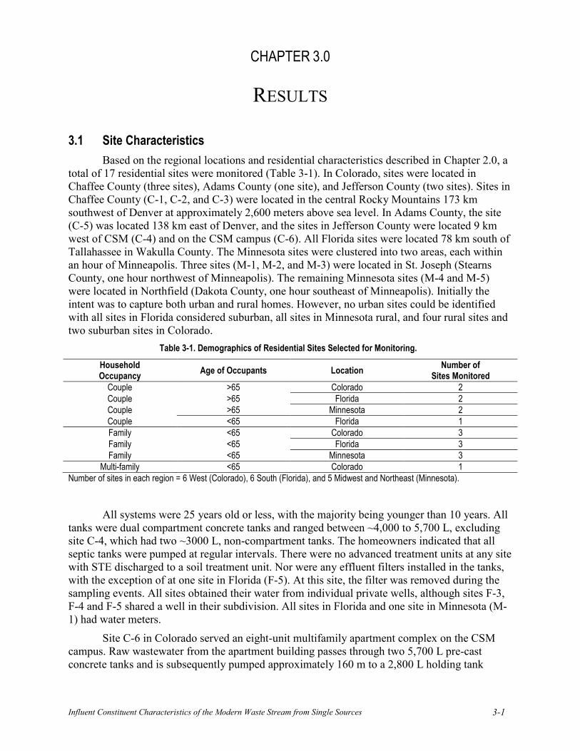
Influent Constituent Characteristics of the Modern Waste Stream from Single Sources 3-1
CHAPTER 3.0
RESULTS 3.1 Site Characteristics
Based on the regional locations and residential characteristics described in Chapter 2.0, a total of 17 residential sites were monitored (Table 3-1). In Colorado, sites were located in Chaffee County (three sites), Adams County (one site), and Jefferson County (two sites). Sites in Chaffee County (C-1, C-2, and C-3) were located in the central Rocky Mountains 173 km southwest of Denver at approximately 2,600 meters above sea level. In Adams County, the site (C-5) was located 138 km east of Denver, and the sites in Jefferson County were located 9 km west of CSM (C-4) and on the CSM campus (C-6). All Florida sites were located 78 km south of Tallahassee in Wakulla County. The Minnesota sites were clustered into two areas, each within an hour of Minneapolis. Three sites (M-1, M-2, and M-3) were located in St. Joseph (Stearns County, one hour northwest of Minneapolis). The remaining Minnesota sites (M-4 and M-5) were located in Northfield (Dakota County, one hour southeast of Minneapolis). Initially the intent was to capture both urban and rural homes. However, no urban sites could be identified with all sites in Florida considered suburban, all sites in Minnesota rural, and four rural sites and two suburban sites in Colorado.
Table 3-1. Demographics of Residential Sites Selected for Monitoring.
Household Occupancy Age of Occupants Location Number of
Sites Monitored Couple >65 Colorado 2 Couple >65 Florida 2 Couple >65 Minnesota 2 Couple <65 Florida 1 Family <65 Colorado 3 Family <65 Florida 3 Family <65 Minnesota 3
Multi-family <65 Colorado 1 Number of sites in each region = 6 West (Colorado), 6 South (Florida), and 5 Midwest and Northeast (Minnesota).
All systems were 25 years old or less, with the majority being younger than 10 years. All tanks were dual compartment concrete tanks and ranged between ~4,000 to 5,700 L, excluding site C-4, which had two ~3000 L, non-compartment tanks. The homeowners indicated that all septic tanks were pumped at regular intervals. There were no advanced treatment units at any site with STE discharged to a soil treatment unit. Nor were any effluent filters installed in the tanks, with the exception of at one site in Florida (F-5). At this site, the filter was removed during the sampling events. All sites obtained their water from individual private wells, although sites F-3, F-4 and F-5 shared a well in their subdivision. All sites in Florida and one site in Minnesota (M-1) had water meters.
Site C-6 in Colorado served an eight-unit multifamily apartment complex on the CSM campus. Raw wastewater from the apartment building passes through two 5,700 L pre-cast concrete tanks and is subsequently pumped approximately 160 m to a 2,800 L holding tank

3-2
located at the Mines Park Test Site. The first 5,700L tank is a single compartment tank and the second 5,700 L tank is a dual compartment tank. For this study, STE was collected at the outlet of the second tank prior to pumping to the holding tank at the Mines Park Test Site. The water source for C-6 is the City of Golden municipal water supply. Because of the differences in C-6, the results are not combined with the other sites in the general analyses of this work, as the waste stream was expected to be different than single source residential sites. It should be noted that C-6 does not include laundry facilities (provided in a separate housing unit at the student housing complex) and there were not replicate multifamily sites in this study. However, when comparisons of the data were made to previously reported literature values, the data from C-6 (noted at “Mines Park”) was also noted.
Each household was given a detailed survey that included questions on water use, personal care products and pharmaceuticals used on a regular basis, OWS specifics (e.g., tank size, age, last pumping of the tank, etc.), and general household questions such as occupancy, number of bedrooms, use of garbage disposal and water softener (Appendix A). A summary of key household characteristics for each site monitored is presented in Table 3-2 and Figure 3-1.
Regional variations in the strength of the waste stream were observed in the Phase 1 Literature Review and may be the result of the different characteristics of the households and/or lifestyle variations in the different regions. These types of variations were observed regionally between the sites monitored for this study (Figure 3-2). For example, all Colorado households in this study reported the use of antibacterial soaps, while only half of the households in Florida and 60% of the households in Minnesota reported use of antibacterial soaps. As another example, all the Florida households in this study had low-flow toilets (6 liters per flush or 1.6 gallons per flush [gpf]), while only 60% of the Colorado and Minnesota households had them. The use of low-flow toilets and other water saving fixtures may make the waste stream stronger. Finally, all the households in Colorado had garbage disposals, while only one site each in Florida and in Minnesota had disposals. As with low-flow fixtures, the use of garbage disposals may affect the strength of the waste stream due to the introduction of ground-up food.
Table 3-2. Characteristics of Residential Sites Selected for Monitoring.
Region Site ID
Number of Occupants
Occupant Age
Number of Bedrooms
Disposal (Y/N)
Water Softener
Age of System
Tank Size (L)
West C-1 5 <65 3 Y N 2001 5,678 (Colorado) C-2 6 <65 8 Y N 2001 3,785
C-3 2 >65 5 Y Y 2006 5,678 C-4 4 <65 4 Y N 1983 two 3,028 tanks C-5 2 >65 2 Y N 2004 3,785 C-6 18 <65 16 Y N 1998 two 5,678 tanks
South F-1 2 <65 3 N N 1999 3,974 (Florida) F-2 4 <65 2 N N 2002 3,974
F-3 2 >65 3 Y N 1999 3,974 F-4 2 >65 3 N Y 1999 3,974 F-5 3 <65 2 N N 2007 3,974 F-6 3 <65 2 N N 1999 3,974
Midwest/Northeast M-1 5 <65 4 N Y 1998 5,034 (Minnesota) M-2 5 <65 3 N N 1994 4,731
M-3 2 >65 3 N Y 1996 3,785 M-4 2 >65 4 Y Y 1987 4,731 M-5 6 <65 6 N Y 1988 4,731
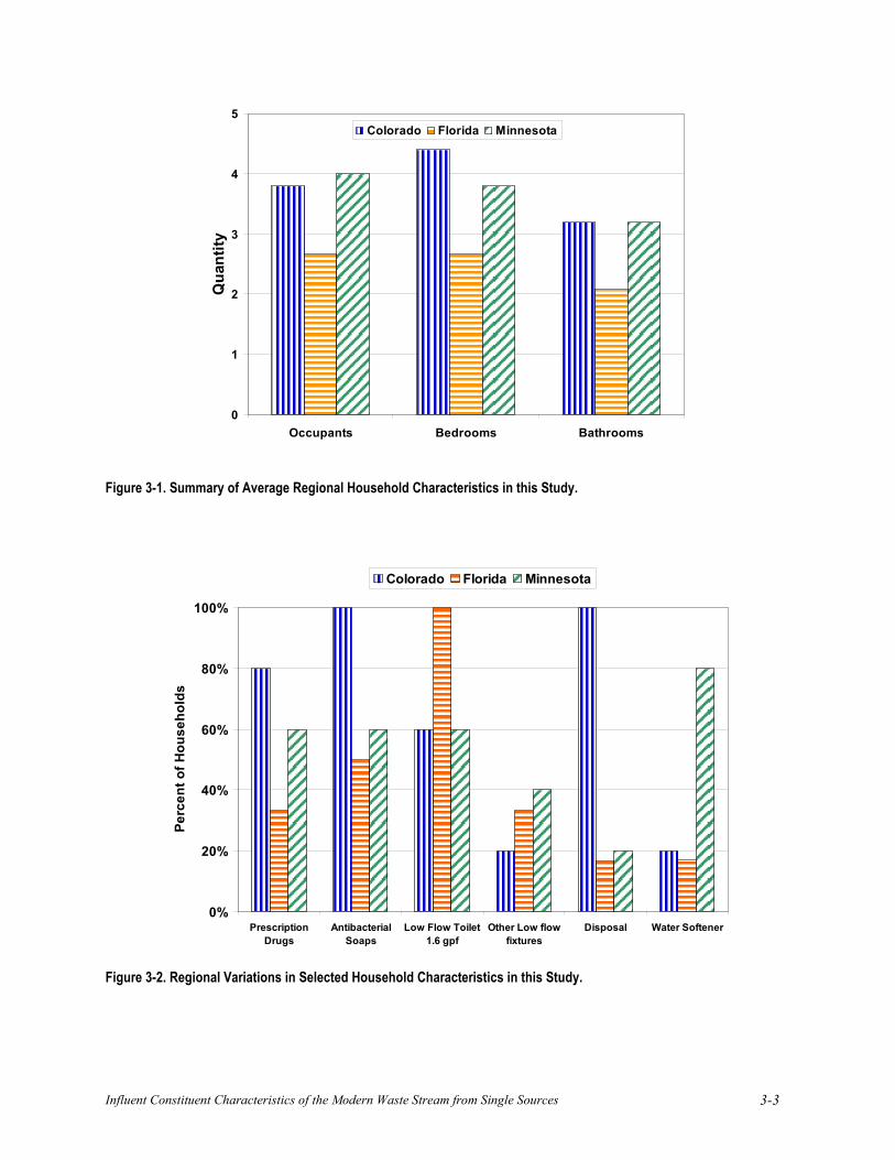
Influent Constituent Characteristics of the Modern Waste Stream from Single Sources 3-3
0
1
2
3
4
5
Occupants Bedrooms Bathrooms
Qua
ntity
Colorado Florida Minnesota
Figure 3-1. Summary of Average Regional Household Characteristics in this Study.
0%
20%
40%
60%
80%
100%
PrescriptionDrugs
AntibacterialSoaps
Low Flow Toilet1.6 gpf
Other Low flowfixtures
Disposal Water Softener
Perc
ent o
f Hou
seho
lds
Colorado Florida Minnesota
Figure 3-2. Regional Variations in Selected Household Characteristics in this Study.

3-4
During the spring sampling round (summer sampling round for C-4), a sample of the source water was also collected at each site and analyzed for Tier 1 constituents excluding cBOD5 and solids. The most noteworthy observation in the source water was the alkalinity concentration, with the highest mean value in Minnesota (262 mg/L as calcium carbonate [CaCO3]), followed by Florida (151 mg/L as CaCO3) and Colorado (103 mg/L as CaCO3) (Table 3-3). Concentrations of all other standard constituents were low or below detection limits (i.e., non-detect). Anions were measured in source water during the summer sampling event using Ion Chromatography, USEPA Method 300.0 using Dionex DX-600 equipped with an AS4A anion exchange column. Several sites had elevated levels of chloride concentrations (C-3, C-5, F-2, F-5, and M-3), at one site (C-5) sulfate concentrations was significantly elevated (617 mg/L), and the nitrate-nitrogen concentration was slightly elevated (1.88 mg-N/L) at C-3 with no explanation available at this time (Table 3-3).
Table 3-3. Selected Household Source Water Tier 1 Characteristics and Anions.
Site ID pH Alkalinity (mg-CaCO3)
Chloride (mg-Cl/L)
Nitrate1 (mg-N/L)
Sulfate (mg-SO4/L)
Spring Summer C-1 7.35 40 0.40 BDL 0.13 17.64 C-2 7.25 44 1.39 BDL 0.52 8.95 C-3 7.44 126 35.34 4.1 1.88 39.71 C-4 7.42 28 6.89 BDL 0.02 3.76 C-5 8.03 202 83.37 BDL 0.05 617.47 C-6* 7.89 37 5.97 BDL 0.08 31.47 F-1 7.83 91 5.87 BDL 0.14 4.58 F-2 7.38 144 50.76 BDL 0.03 15.22 F-3 7.60 176 5.49 BDL 0.08 22.15 F-4 7.89 174 5.01 BDL 0.01 4.78 F-5 7.46 136 54.88 BDL 0.03 15.43 F-6 7.81 185 5.09 BDL 0.02 6.04 M-1 7.65 330 1.00 BDL 0.02 15.49 M-2 7.44 220 1.26 BDL 0.04 9.40 M-3 7.43 188 34.76 16.9 0.16 44.19 M-4 7.25 304 1.55 BDL 0.02 6.74 M-5 7.43 268 9.56 BDL 0.03 33.96
1 Nitrate-nitrogen analyzed by photospectrameter in Spring and by ion chromatography in Summer. BDL = below detection limit. * Mines Park multifamily housing unit.
The source water was also analyzed for cations (using Inductively-Coupled Plasma Atomic Emission Spectroscopy) during the spring and summer sampling rounds (Table 3-4). The most noteworthy results indicate the use of water softeners at three sites, C-3 (potassium based water softener), and F-4 and M-1 (sodium based water softeners). Elevated levels of cations at the other sites in Minnesota where water softeners are used (M-3, M4, and M-5) were not observed. Only sites C-3 and M-3 returned the water softener backwash cycle to the tank. There is no explanation for the high levels of sodium in the source water at site C-5.

Influent Constituent Characteristics of the Modern Waste Stream from Single Sources 3-5
Table 3-4. Selected Cations Present in the Household Source Water (mg/L).
Site Calcium Potassium Magnesium Manganese Sodium ID Spr Sum Spr Sum Spr Sum Spr Sum Spr Sum
C-1 15.15 15.23 BDL BDL 2.16 2.17 0.0007 0.0119 3.28 3.39 C-2 14.98 14.38 1.83 BDL 2.33 2.33 BDL 0.0116 7.53 8.00 C-3 0.21 0.32 119.50 95.58 0.04 0.15 BDL 0.0004 41.42 35.73 C-4 BDL 8.07 BDL 1.24 BDL 2.25 BDL 0.0207 BDL 8.07 C-5 38.69 38.79 7.38 3.98 6.75 6.73 0.0340 0.0412 349.45 332.58 C-6* 37.09 15.30 3.30 3.36 9.20 3.69 0.0028 0.0042 29.70 15.92 F-1 39.28 37.54 BDL BDL BDL BDL 0.0007 0.0014 2.50 3.14 F-2 52.67 52.04 BDL BDL 11.09 9.69 0.0082 0.0100 42.72 29.21 F-3 BDL 49.75 BDL BDL BDL 6.71 BDL 0.0003 BDL 14.22 F-4 0.27 0.12 BDL BDL 0.03 0.04 0.0009 0.0003 92.15 81.38 F-5 50.23 50.89 BDL BDL 10.35 10.18 0.0091 0.0397 40.79 32.18 F-6 BDL 58.59 BDL BDL BDL 7.88 BDL 0.0003 BDL 4.73 M-1 0.41 0.65 BDL BDL BDL BDL 0.0015 0.0020 146.30 151.21 M-2 60.16 46.21 2.75 2.54 16.05 12.93 0.1708 0.0937 1.57 4.27 M-3 94.56 90.43 3.96 3.61 28.95 27.26 0.0381 0.1310 21.35 22.03 M-4 77.75 83.02 6.75 2.06 27.10 29.35 0.1346 0.1431 2.90 4.37 M-5 84.08 73.09 3.65 1.96 29.18 26.08 0.2324 0.2086 1.70 2.79
BDL = below detection limit. * Mines Park multifamily housing unit.
3.2 Tier 1: Conventional Constituents Tier 1 conventional constituents of interest were analyzed in all raw wastewater and STE
samples collected to obtain basic information on residential OWS. These Tier 1 constituents included daily indoor water use (flow), pH, alkalinity, TS, TSS, cBOD5, COD, TOC, DOC, total nitrogen, ammonium-nitrogen, nitrate-nitrogen, total phosphorous, and fecal coliform bacteria. Comparison of Tier 1 values measured in this study to the values reported in the Phase 1 Literature Review are provided in Appendix B. Descriptive statistics as well as regional, seasonal, and age of occupant comparisons are also presented in Appendix B.
3.2.1 Flow Household water use is an important parameter used for design of OWS and is often
based on an estimated per capita occupancy of the bedrooms and some expected median per capita water use value. A conservative peak factor is then often used (e.g., 1.5 times the average design flow) to ensure performance during high or peak flow periods. This design approach often leads to conservatively oversized tanks and soil treatment units and the additional associated costs to the homeowner. A clear understanding of actual interior water use is crucial to enable OWS designers and decision makers to evaluate various potential designs and performance implications.
In this study, the volume of water used during each 24-hour sampling event was measured with a flow meter installed after the macerating vacuum pump. Consequently, all indoor water use was measured. To ensure the accuracy of the flow meter the readings were compared to flow meters installed on the source water inlet line at seven residences (six in Florida and one in Minnesota). During the test, the homeowners were asked to not use any source water for outdoor activities. The flow meter installed after the macerating vacuum pump slightly under-estimated the water use by 1-5%.
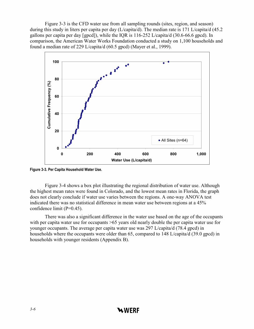
3-6
Figure 3-3 is the CFD water use from all sampling rounds (sites, region, and season) during this study in liters per capita per day (L/capita/d). The median rate is 171 L/capita/d (45.2 gallons per capita per day [gpcd]), while the IQR is 116-252 L/capita/d (30.6-66.6 gpcd). In comparison, the American Water Works Foundation conducted a study on 1,100 households and found a median rate of 229 L/capita/d (60.5 gpcd) (Mayer et al., 1999).
0
20
40
60
80
100
0 200 400 600 800 1,000Water Use (L/capita/d)
Cum
ulat
ive
Freq
uenc
y (%
)
All Sites (n=64)
Figure 3-3. Per Capita Household Water Use.
Figure 3-4 shows a box plot illustrating the regional distribution of water use. Although the highest mean rates were found in Colorado, and the lowest mean rates in Florida, the graph does not clearly conclude if water use varies between the regions. A one-way ANOVA test indicated there was no statistical difference in mean water use between regions at a 45% confidence limit (P=0.45).
There was also a significant difference in the water use based on the age of the occupants with per capita water use for occupants >65 years old nearly double the per capita water use for younger occupants. The average per capita water use was 297 L/capita/d (78.4 gpcd) in households where the occupants were older than 65, compared to 148 L/capita/d (39.0 gpcd) in households with younger residents (Appendix B).
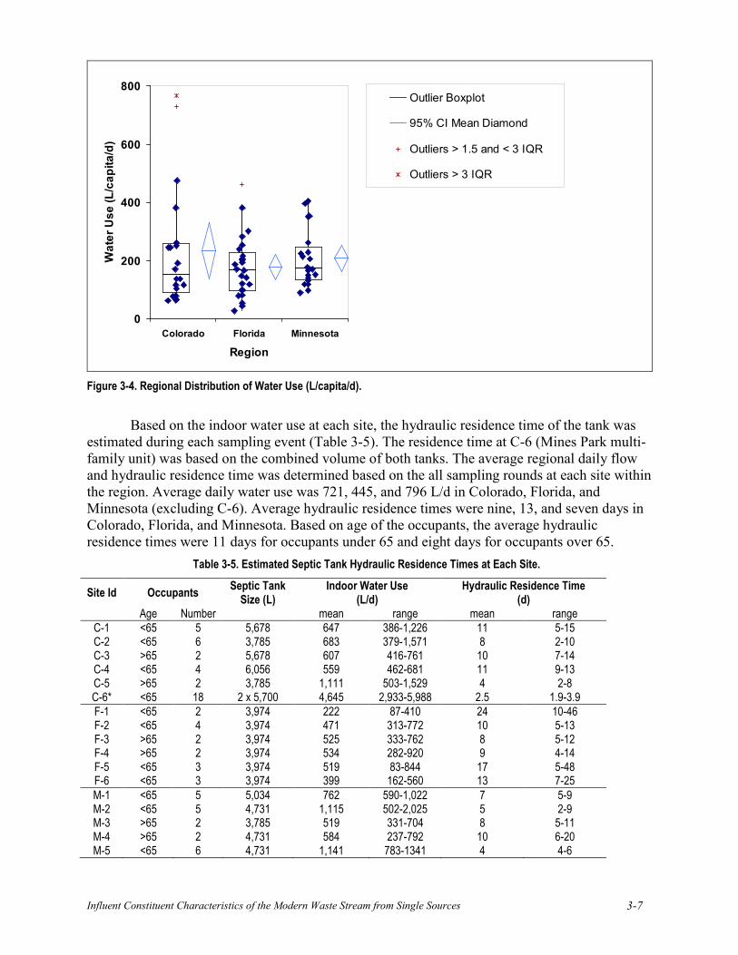
Influent Constituent Characteristics of the Modern Waste Stream from Single Sources 3-7
0
200
400
600
800
Colorado Florida Minnesota
Region
Wat
er U
se (L
/cap
ita/d
)Outlier Boxplot
95% CI Mean Diamond
Outliers > 1.5 and < 3 IQR
Outliers > 3 IQR
Figure 3-4. Regional Distribution of Water Use (L/capita/d).
Based on the indoor water use at each site, the hydraulic residence time of the tank was estimated during each sampling event (Table 3-5). The residence time at C-6 (Mines Park multi-family unit) was based on the combined volume of both tanks. The average regional daily flow and hydraulic residence time was determined based on the all sampling rounds at each site within the region. Average daily water use was 721, 445, and 796 L/d in Colorado, Florida, and Minnesota (excluding C-6). Average hydraulic residence times were nine, 13, and seven days in Colorado, Florida, and Minnesota. Based on age of the occupants, the average hydraulic residence times were 11 days for occupants under 65 and eight days for occupants over 65.
Table 3-5. Estimated Septic Tank Hydraulic Residence Times at Each Site.
Site Id Occupants Septic Tank Size (L)
Indoor Water Use (L/d)
Hydraulic Residence Time (d)
Age Number mean range mean range C-1 <65 5 5,678 647 386-1,226 11 5-15 C-2 <65 6 3,785 683 379-1,571 8 2-10 C-3 >65 2 5,678 607 416-761 10 7-14 C-4 <65 4 6,056 559 462-681 11 9-13 C-5 >65 2 3,785 1,111 503-1,529 4 2-8 C-6* <65 18 2 x 5,700 4,645 2,933-5,988 2.5 1.9-3.9 F-1 <65 2 3,974 222 87-410 24 10-46 F-2 <65 4 3,974 471 313-772 10 5-13 F-3 >65 2 3,974 525 333-762 8 5-12 F-4 >65 2 3,974 534 282-920 9 4-14 F-5 <65 3 3,974 519 83-844 17 5-48 F-6 <65 3 3,974 399 162-560 13 7-25 M-1 <65 5 5,034 762 590-1,022 7 5-9 M-2 <65 5 4,731 1,115 502-2,025 5 2-9 M-3 >65 2 3,785 519 331-704 8 5-11 M-4 >65 2 4,731 584 237-792 10 6-20 M-5 <65 6 4,731 1,141 783-1341 4 4-6

3-8
To gain a better understanding of the specific types of water use during each sampling event, the homeowners were asked to record all specific water use activities during the sampling period (toilet flushes, showers, washing machine loads, dishwasher loads, teeth brushing etc.) (Table 3-6). Figure 3-5 illustrates the average number of specific events per capita per day, within each region (note the logarithmic scale on the y-axis). It is interesting to note that toilet flushes, hand washes and teeth brushing account for the greatest average number of events per capita (Table 3-6). If each flush is assumed to average 8 L, each hand wash and teeth brushing event 3 L each, then those events could account for approximately 60 L of the daily water use, or one third of all water use (assuming an average of 171 L/capita/day [45.2 gpcd]).
Table 3-6. Summary of Regional Water Use (Average Number of Events/capita/d).
Colorado Florida Minnesota Showers 0.9 0.6 0.4 Baths 0.0 0.1 0.2 Toilet flush 5.7 5.2 4.3 Toilet cleaning 0.0 0.0 0.1 Hand wash 5.4 2.0 4.8 Sink cleaning 0.2 0.1 0.1 Teeth brushing 1.8 1.2 1.4 Dishwasher 0.3 0.3 0.3 Dishwashing in sink 0.1 0.1 0.7 Misc. sink use 0.1 0.2 0.2 Laundry 0.6 0.3 0.4
0.01
0.1
1
10
ShowersBath
s
Toilet fl
ush
Toilet c
leaning
Hand w
ash
Sink clea
ning
Teeth bru
shing
Dishwas
her
Dishwas
hing in si
nk
Misc si
nk use
Laundry
Wat
er U
se (e
vent
s/ca
pita
/day
)
Colorado Florida Minnesota
Figure 3-5. Regional Water Use Events.

Influent Constituent Characteristics of the Modern Waste Stream from Single Sources 3-9
Alternatively, Figure 3-6 shows the percent of a specific event that occurred within each region of the total number of events during this study. The figure suggests subtle differences in household activities within the regions during this study (Colorado showered the most while Minnesota took the most baths). By depicting the data in this manner, household flow in various regions can be estimated using typical values for water use from various devices as reported by Crites and Tchobanoglous (1998). For example, based on the data from representative Colorado sites (Table 3-6) using standard dishwashers and laundry machines (i.e., not low flow) and 6 L toilets (1.6 gpf), water use per capita can be estimated as:
Flow (L/capita/d) = 0.3*23 L (dishwasher) + 0.6*151 L (laundry) + 0.4*4 L (misc. water use) + 0.9*76 L (shower) + 5.7*6 L (toilet) + 5.4*4 L (hand wash) + 1.8*4 L (teeth brushing)
This example suggests water use of approximately 230 L/capita/d (~60 gal/capita/d) which is similar to the average water use per resident in Colorado (234 L/capita/d [61.8 gpcd]) and within the IQR of all the water use from this study (Appendix B).
0%
20%
40%
60%
80%
100%
ShowersBath
s
Toilet fl
ush
Toilet c
leaning
Hand w
ash
Sink clea
ning
Teeth bru
shing
Dishwas
her
Dishwas
hing in si
nk
Misc si
nk use
Laundry
Perc
ent o
f all
even
ts
Colorado Florida Minnesota
Figure 3-6. Percentage of the Total Water Use Events Recorded in this Study that Occurred within Each Region.
3.2.2 pH A hydrogen-ion (H+) concentration in solution is typically expressed in terms of pH,
which is defined as the negative logarithm of the hydrogen-ion concentration. In OWS, pH is a useful parameter to assess the ionic activity, the predominant form of nitrogen in the wastewater (ammonia >9.3 vs. ammonium at <9.3), as well as the likelihood of microbial treatment of the wastewater (optimum pH between 5 and 9).
The pH values in the raw wastewater were found to range between 6.4-10.1, with an average and median value of 8.1 (Figure 3-7). The high value of 10.1 may be an outlier, as the
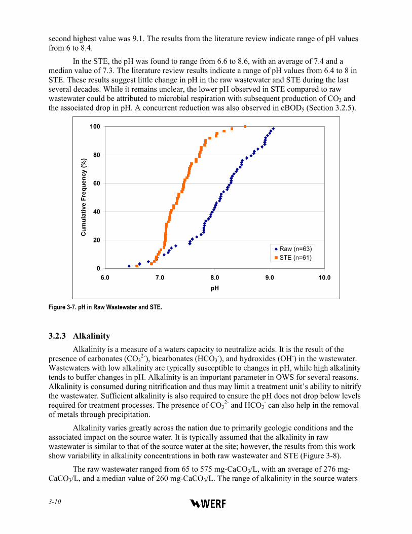
3-10
second highest value was 9.1. The results from the literature review indicate range of pH values from 6 to 8.4.
In the STE, the pH was found to range from 6.6 to 8.6, with an average of 7.4 and a median value of 7.3. The literature review results indicate a range of pH values from 6.4 to 8 in STE. These results suggest little change in pH in the raw wastewater and STE during the last several decades. While it remains unclear, the lower pH observed in STE compared to raw wastewater could be attributed to microbial respiration with subsequent production of CO2 and the associated drop in pH. A concurrent reduction was also observed in cBOD5 (Section 3.2.5).
0
20
40
60
80
100
6.0 7.0 8.0 9.0 10.0pH
Cum
ulat
ive
Freq
uenc
y (%
)
Raw (n=63)STE (n=61)
Figure 3-7. pH in Raw Wastewater and STE.
3.2.3 Alkalinity Alkalinity is a measure of a waters capacity to neutralize acids. It is the result of the
presence of carbonates (CO32-), bicarbonates (HCO3
-), and hydroxides (OH-) in the wastewater. Wastewaters with low alkalinity are typically susceptible to changes in pH, while high alkalinity tends to buffer changes in pH. Alkalinity is an important parameter in OWS for several reasons. Alkalinity is consumed during nitrification and thus may limit a treatment unit’s ability to nitrify the wastewater. Sufficient alkalinity is also required to ensure the pH does not drop below levels required for treatment processes. The presence of CO3
2- and HCO3- can also help in the removal
of metals through precipitation.
Alkalinity varies greatly across the nation due to primarily geologic conditions and the associated impact on the source water. It is typically assumed that the alkalinity in raw wastewater is similar to that of the source water at the site; however, the results from this work show variability in alkalinity concentrations in both raw wastewater and STE (Figure 3-8).
The raw wastewater ranged from 65 to 575 mg-CaCO3/L, with an average of 276 mg-CaCO3/L, and a median value of 260 mg-CaCO3/L. The range of alkalinity in the source waters
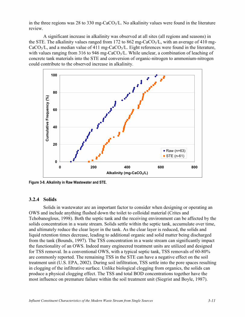
Influent Constituent Characteristics of the Modern Waste Stream from Single Sources 3-11
in the three regions was 28 to 330 mg-CaCO3/L. No alkalinity values were found in the literature review.
A significant increase in alkalinity was observed at all sites (all regions and seasons) in the STE. The alkalinity values ranged from 172 to 862 mg-CaCO3/L, with an average of 410 mg-CaCO3/L, and a median value of 411 mg-CaCO3/L. Eight references were found in the literature, with values ranging from 316 to 946 mg-CaCO3/L. While unclear, a combination of leaching of concrete tank materials into the STE and conversion of organic-nitrogen to ammonium-nitrogen could contribute to the observed increase in alkalinity.
0
20
40
60
80
100
0 200 400 600 800Alkalinity (mg-CaCO3/L)
Cum
ulat
ive
Freq
uenc
y (%
)
Raw (n=63)STE (n-61)
Figure 3-8. Alkalinity in Raw Wastewater and STE.
3.2.4 Solids Solids in wastewater are an important factor to consider when designing or operating an
OWS and include anything flushed down the toilet to colloidal material (Crites and Tchobanoglous, 1998). Both the septic tank and the receiving environment can be affected by the solids concentration in a waste stream. Solids settle within the septic tank, accumulate over time, and ultimately reduce the clear layer in the tank. As the clear layer is reduced, the solids and liquid retention times decrease, leading to additional organic and solid matter being discharged from the tank (Bounds, 1997). The TSS concentration in a waste stream can significantly impact the functionality of an OWS. Indeed many engineered treatment units are utilized and designed for TSS removal. In a conventional OWS, with a typical septic tank, TSS removals of 60-80% are commonly reported. The remaining TSS in the STE can have a negative effect on the soil treatment unit (U.S. EPA, 2002). During soil infiltration, TSS settle into the pore spaces resulting in clogging of the infiltrative surface. Unlike biological clogging from organics, the solids can produce a physical clogging effect. The TSS and total BOD concentrations together have the most influence on premature failure within the soil treatment unit (Siegrist and Boyle, 1987).
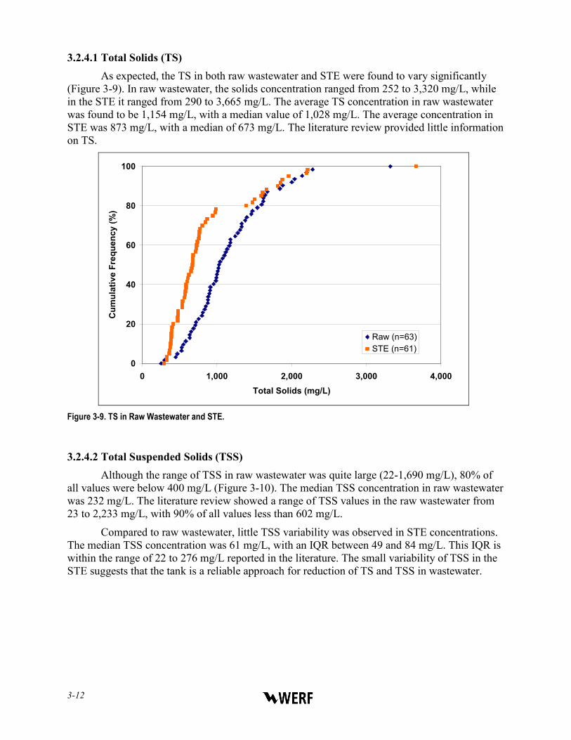
3-12
3.2.4.1 Total Solids (TS) As expected, the TS in both raw wastewater and STE were found to vary significantly
(Figure 3-9). In raw wastewater, the solids concentration ranged from 252 to 3,320 mg/L, while in the STE it ranged from 290 to 3,665 mg/L. The average TS concentration in raw wastewater was found to be 1,154 mg/L, with a median value of 1,028 mg/L. The average concentration in STE was 873 mg/L, with a median of 673 mg/L. The literature review provided little information on TS.
0
20
40
60
80
100
0 1,000 2,000 3,000 4,000Total Solids (mg/L)
Cum
ulat
ive
Freq
uenc
y (%
)
Raw (n=63)STE (n=61)
Figure 3-9. TS in Raw Wastewater and STE.
3.2.4.2 Total Suspended Solids (TSS) Although the range of TSS in raw wastewater was quite large (22-1,690 mg/L), 80% of
all values were below 400 mg/L (Figure 3-10). The median TSS concentration in raw wastewater was 232 mg/L. The literature review showed a range of TSS values in the raw wastewater from 23 to 2,233 mg/L, with 90% of all values less than 602 mg/L.
Compared to raw wastewater, little TSS variability was observed in STE concentrations. The median TSS concentration was 61 mg/L, with an IQR between 49 and 84 mg/L. This IQR is within the range of 22 to 276 mg/L reported in the literature. The small variability of TSS in the STE suggests that the tank is a reliable approach for reduction of TS and TSS in wastewater.
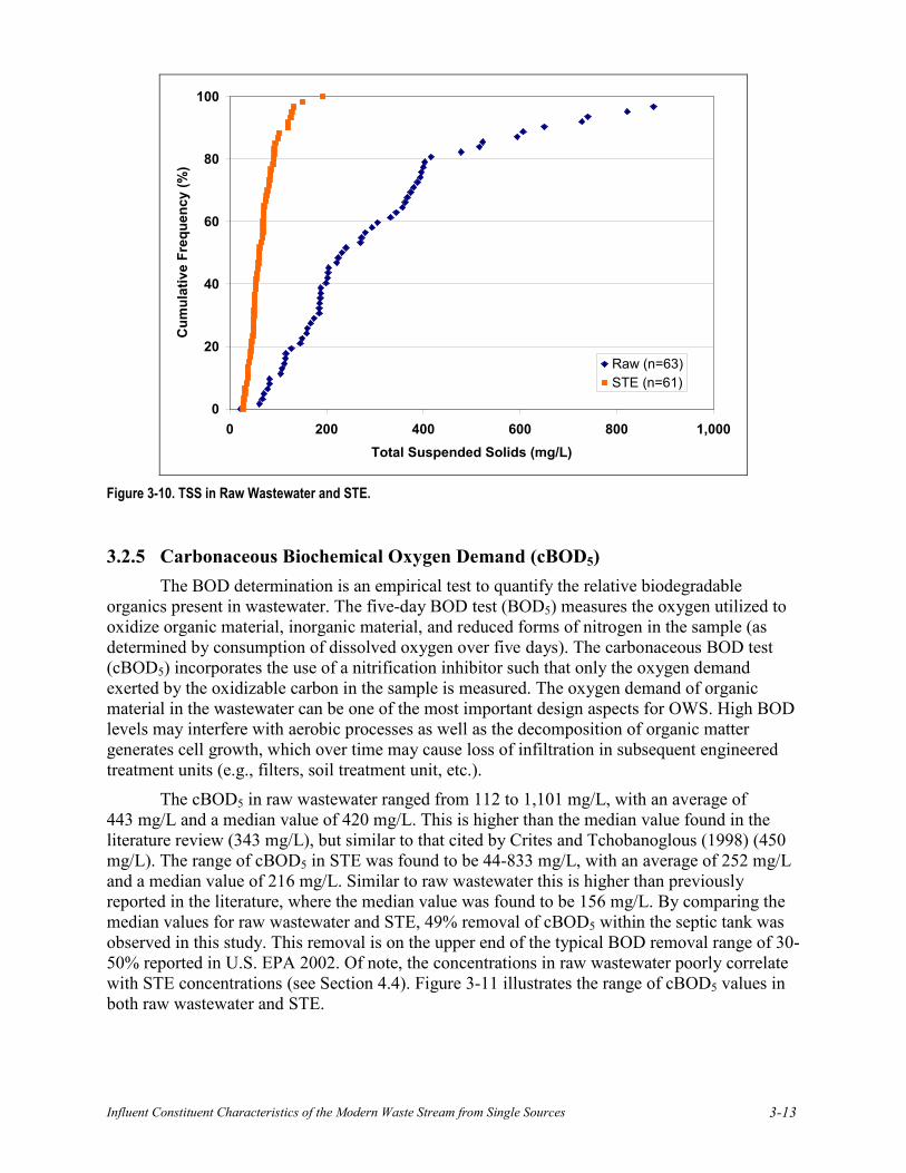
Influent Constituent Characteristics of the Modern Waste Stream from Single Sources 3-13
0
20
40
60
80
100
0 200 400 600 800 1,000Total Suspended Solids (mg/L)
Cum
ulat
ive
Freq
uenc
y (%
)
Raw (n=63)STE (n=61)
Figure 3-10. TSS in Raw Wastewater and STE.
3.2.5 Carbonaceous Biochemical Oxygen Demand (cBOD5) The BOD determination is an empirical test to quantify the relative biodegradable
organics present in wastewater. The five-day BOD test (BOD5) measures the oxygen utilized to oxidize organic material, inorganic material, and reduced forms of nitrogen in the sample (as determined by consumption of dissolved oxygen over five days). The carbonaceous BOD test (cBOD5) incorporates the use of a nitrification inhibitor such that only the oxygen demand exerted by the oxidizable carbon in the sample is measured. The oxygen demand of organic material in the wastewater can be one of the most important design aspects for OWS. High BOD levels may interfere with aerobic processes as well as the decomposition of organic matter generates cell growth, which over time may cause loss of infiltration in subsequent engineered treatment units (e.g., filters, soil treatment unit, etc.).
The cBOD5 in raw wastewater ranged from 112 to 1,101 mg/L, with an average of 443 mg/L and a median value of 420 mg/L. This is higher than the median value found in the literature review (343 mg/L), but similar to that cited by Crites and Tchobanoglous (1998) (450 mg/L). The range of cBOD5 in STE was found to be 44-833 mg/L, with an average of 252 mg/L and a median value of 216 mg/L. Similar to raw wastewater this is higher than previously reported in the literature, where the median value was found to be 156 mg/L. By comparing the median values for raw wastewater and STE, 49% removal of cBOD5 within the septic tank was observed in this study. This removal is on the upper end of the typical BOD removal range of 30-50% reported in U.S. EPA 2002. Of note, the concentrations in raw wastewater poorly correlate with STE concentrations (see Section 4.4). Figure 3-11 illustrates the range of cBOD5 values in both raw wastewater and STE.
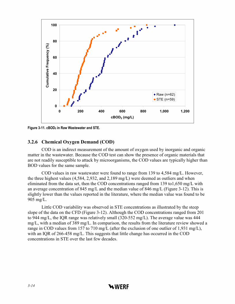
3-14
0
20
40
60
80
100
0 200 400 600 800 1,000 1,200cBOD5 (mg/L)
Cum
ulat
ive
Freq
uenc
y (%
)
Raw (n=62)STE (n=59)
Figure 3-11. cBOD5 in Raw Wastewater and STE.
3.2.6 Chemical Oxygen Demand (COD)
COD is an indirect measurement of the amount of oxygen used by inorganic and organic matter in the wastewater. Because the COD test can show the presence of organic materials that are not readily susceptible to attack by microorganisms, the COD values are typically higher than BOD values for the same sample.
COD values in raw wastewater were found to range from 139 to 4,584 mg/L. However, the three highest values (4,584, 2,932, and 2,189 mg/L) were deemed as outliers and when eliminated from the data set, then the COD concentrations ranged from 139 to1,650 mg/L with an average concentration of 845 mg/L and the median value of 846 mg/L (Figure 3-12). This is slightly lower than the values reported in the literature, where the median value was found to be 905 mg/L.
Little COD variability was observed in STE concentrations as illustrated by the steep slope of the data on the CFD (Figure 3-12). Although the COD concentrations ranged from 201 to 944 mg/L, the IQR range was relatively small (320-552 mg/L). The average value was 444 mg/L, with a median of 389 mg/L. In comparison, the results from the literature review showed a range in COD values from 157 to 710 mg/L (after the exclusion of one outlier of 1,931 mg/L), with an IQR of 266-458 mg/L. This suggests that little change has occurred in the COD concentrations in STE over the last few decades.

Influent Constituent Characteristics of the Modern Waste Stream from Single Sources 3-15
0
20
40
60
80
100
0 500 1,000 1,500 2,000COD (mg/L)
Cum
ulat
ive
Freq
uenc
y (%
)
Raw (n=63)STE (n=60)
Figure 3-12. COD in Raw Wastewater and STE.
3.2.7 Total Organic Carbon (TOC) and Dissolved Organic Carbon (DOC) Organic matter plays an important role in the environment as it affects biochemical
processes, nutrient cycling, chemical transport and interactions. Organic matter content is typically measured as either TOC (unfiltered sample) or DOC (fraction of DOC that passes through a 0.45μm filter). Both the TOC and DOC analyses are fast and accurate tests for assessing the carbon content in wastewater. However, they do not provide the same insight into the wastewater composition as either BOD or COD. For this reason, limited information was present in the existing literature related to TOC and DOC concentrations in raw wastewater and STE: 1 reference for TOC in raw wastewater, 11 references for TOC in STE, no references for DOC in raw wastewater, and 3 references for DOC in STE.
The TOC concentrations in raw wastewater ranged from 35 to 738 mg/L, with an average of 202 mg/L and a median value of 183 mg/L (Figure 3-13). The range is much greater than that reported by Crites and Tchobanoglous (1998) for untreated wastewater (80-290 mg/L) or in the literature (121 mg/L, Edvardsson and Spears, 2000). The range of values in STE was 50-243 mg/L, with an average of 111 mg/L and a median value of 105 mg/L. These values agree with the results of the literature review, where the concentrations ranged from 41 to 147 mg/L.
The DOC concentrations in raw wastewater ranged from 29 to 679 mg/L, with an average of 138 mg/L and a median value of 109 mg/L (Figure 3-14). The range of values in STE was 22-140 mg/L, with an average of 73 mg/L and a median value of 66 mg/L.
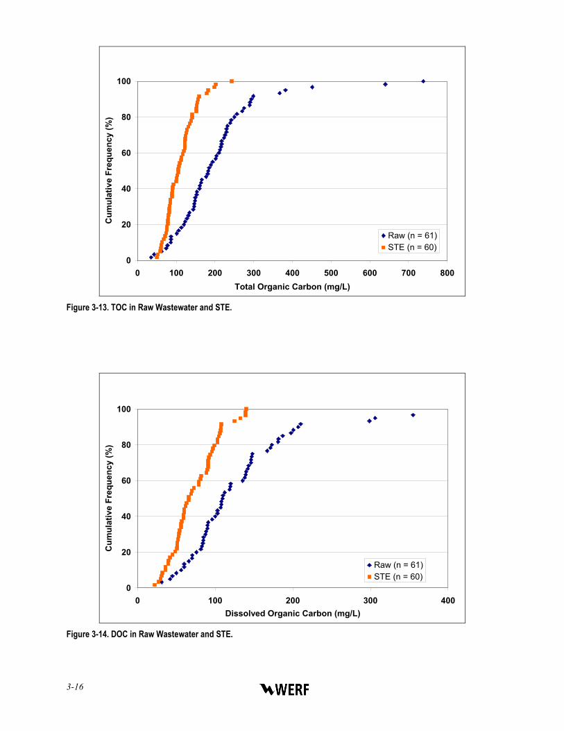
3-16
0
20
40
60
80
100
0 100 200 300 400 500 600 700 800Total Organic Carbon (mg/L)
Cum
ulat
ive
Freq
uenc
y (%
)
Raw (n = 61)STE (n = 60)
Figure 3-13. TOC in Raw Wastewater and STE.
0
20
40
60
80
100
0 100 200 300 400Dissolved Organic Carbon (mg/L)
Cum
ulat
ive
Freq
uenc
y (%
)
Raw (n = 61)STE (n = 60)
Figure 3-14. DOC in Raw Wastewater and STE.
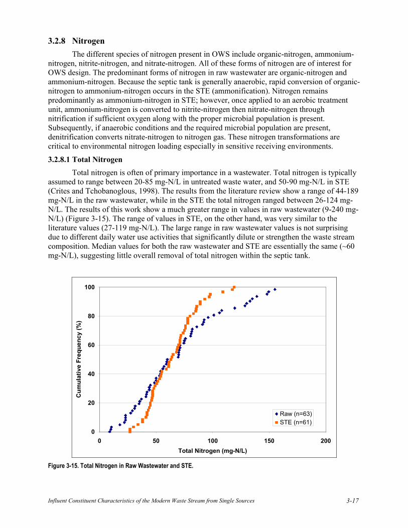
Influent Constituent Characteristics of the Modern Waste Stream from Single Sources 3-17
3.2.8 Nitrogen The different species of nitrogen present in OWS include organic-nitrogen, ammonium-
nitrogen, nitrite-nitrogen, and nitrate-nitrogen. All of these forms of nitrogen are of interest for OWS design. The predominant forms of nitrogen in raw wastewater are organic-nitrogen and ammonium-nitrogen. Because the septic tank is generally anaerobic, rapid conversion of organic-nitrogen to ammonium-nitrogen occurs in the STE (ammonification). Nitrogen remains predominantly as ammonium-nitrogen in STE; however, once applied to an aerobic treatment unit, ammonium-nitrogen is converted to nitrite-nitrogen then nitrate-nitrogen through nitrification if sufficient oxygen along with the proper microbial population is present. Subsequently, if anaerobic conditions and the required microbial population are present, denitrification converts nitrate-nitrogen to nitrogen gas. These nitrogen transformations are critical to environmental nitrogen loading especially in sensitive receiving environments.
3.2.8.1 Total Nitrogen Total nitrogen is often of primary importance in a wastewater. Total nitrogen is typically
assumed to range between 20-85 mg-N/L in untreated waste water, and 50-90 mg-N/L in STE (Crites and Tchobanoglous, 1998). The results from the literature review show a range of 44-189 mg-N/L in the raw wastewater, while in the STE the total nitrogen ranged between 26-124 mg-N/L. The results of this work show a much greater range in values in raw wastewater (9-240 mg-N/L) (Figure 3-15). The range of values in STE, on the other hand, was very similar to the literature values (27-119 mg-N/L). The large range in raw wastewater values is not surprising due to different daily water use activities that significantly dilute or strengthen the waste stream composition. Median values for both the raw wastewater and STE are essentially the same (~60 mg-N/L), suggesting little overall removal of total nitrogen within the septic tank.
0
20
40
60
80
100
0 50 100 150 200Total Nitrogen (mg-N/L)
Cum
ulat
ive
Freq
uenc
y (%
)
Raw (n=63)STE (n=61)
Figure 3-15. Total Nitrogen in Raw Wastewater and STE.
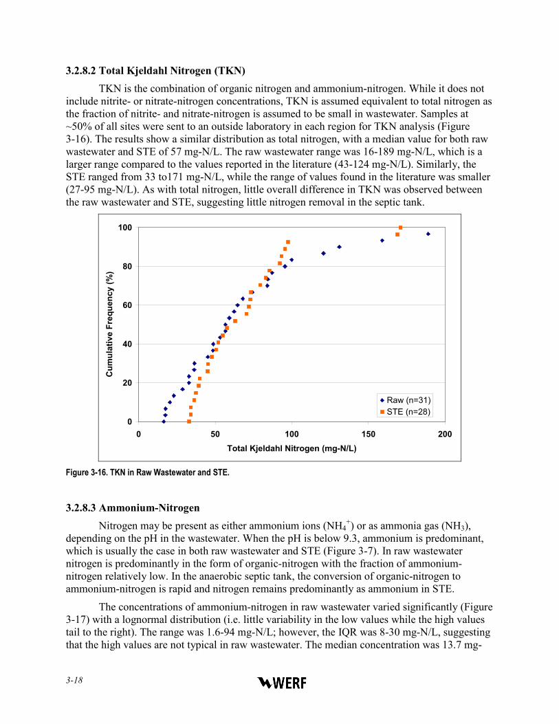
3-18
3.2.8.2 Total Kjeldahl Nitrogen (TKN) TKN is the combination of organic nitrogen and ammonium-nitrogen. While it does not
include nitrite- or nitrate-nitrogen concentrations, TKN is assumed equivalent to total nitrogen as the fraction of nitrite- and nitrate-nitrogen is assumed to be small in wastewater. Samples at ~50% of all sites were sent to an outside laboratory in each region for TKN analysis (Figure 3-16). The results show a similar distribution as total nitrogen, with a median value for both raw wastewater and STE of 57 mg-N/L. The raw wastewater range was 16-189 mg-N/L, which is a larger range compared to the values reported in the literature (43-124 mg-N/L). Similarly, the STE ranged from 33 to171 mg-N/L, while the range of values found in the literature was smaller (27-95 mg-N/L). As with total nitrogen, little overall difference in TKN was observed between the raw wastewater and STE, suggesting little nitrogen removal in the septic tank.
0
20
40
60
80
100
0 50 100 150 200Total Kjeldahl Nitrogen (mg-N/L)
Cum
ulat
ive
Freq
uenc
y (%
)
Raw (n=31)STE (n=28)
Figure 3-16. TKN in Raw Wastewater and STE.
3.2.8.3 Ammonium-Nitrogen Nitrogen may be present as either ammonium ions (NH4
+) or as ammonia gas (NH3), depending on the pH in the wastewater. When the pH is below 9.3, ammonium is predominant, which is usually the case in both raw wastewater and STE (Figure 3-7). In raw wastewater nitrogen is predominantly in the form of organic-nitrogen with the fraction of ammonium-nitrogen relatively low. In the anaerobic septic tank, the conversion of organic-nitrogen to ammonium-nitrogen is rapid and nitrogen remains predominantly as ammonium in STE.
The concentrations of ammonium-nitrogen in raw wastewater varied significantly (Figure 3-17) with a lognormal distribution (i.e. little variability in the low values while the high values tail to the right). The range was 1.6-94 mg-N/L; however, the IQR was 8-30 mg-N/L, suggesting that the high values are not typical in raw wastewater. The median concentration was 13.7 mg-

Influent Constituent Characteristics of the Modern Waste Stream from Single Sources 3-19
N/L. Ammonium-nitrogen results from the literature review ranged from 8.8 to 154 mg-N/L with an IQR of 27-53 mg-N/L, and a median value of 47 mg-N/L. The large discrepancy in median values between this study and the literature review may be due to the limited number of studies (n=12) previously reported in the literature.
Ammonium-nitrogen in STE ranged from 25 to 112 mg-N/L, with an IQR of 42-68 mg-N/L. The average value was 56 mg-N/L and the median 53 mg-N/L. Seventy-eight literature studies reported ammonium-nitrogen concentrations in STE ranging from 0-96 mg-N/L, with an IQR of 28-44 mg-N/L, and a median value of 36 mg-N/L. The results of this work suggest that ammonium-nitrogen concentrations are higher in STE than may have been previously assumed.
0
20
40
60
80
100
0 20 40 60 80 100 120Ammonium-Nitrogen (mg-N/L)
Cum
ulat
ive
Freq
uenc
y (%
)
Raw (n=63)STE (n=61)
Figure 3-17. Ammonium-nitrogen in Raw Wastewater and STE.
3.2.8.4 Nitrate-Nitrogen Information on nitrate-nitrogen concentrations in OWS are of utmost concern as nitrate
contaminated drinking waters has been linked to various illnesses (methemoglobinemia) and environmental concerns. Unlike other Tier 1 constituents, a drinking water standard has been established for nitrate-nitrogen (10 mg-N/L). Although the largest fraction of nitrogen in STE is in the form of ammonium-nitrogen with little to no nitrate-nitrogen present, the ammonium-nitrogen is either sorbed or converted to nitrate-nitrogen once applied to the soil treatment unit.
The concentrations of nitrate-nitrogen in raw wastewater ranged from below detection limits (0.2 mg-N/L) to 8.5 mg-N/L, with an average of 2.1 mg-N/L and a median value of 1.9 mg-N/L (Figure 3-18). These values are higher than previously reported in the literature (below detection limits to 1.1 mg-N/L). Although the range in concentrations in the STE was 0.1-7.1 mg-N/L, little overall variability existed (if outliers were excluded). This is clearly shown by the IQR of 0.6-1.1 mg-N/L. The literature review showed a similar range in values (0-10.3 mg-N/L), although the IQR was lower (0.05-0.7 mg-N/L).
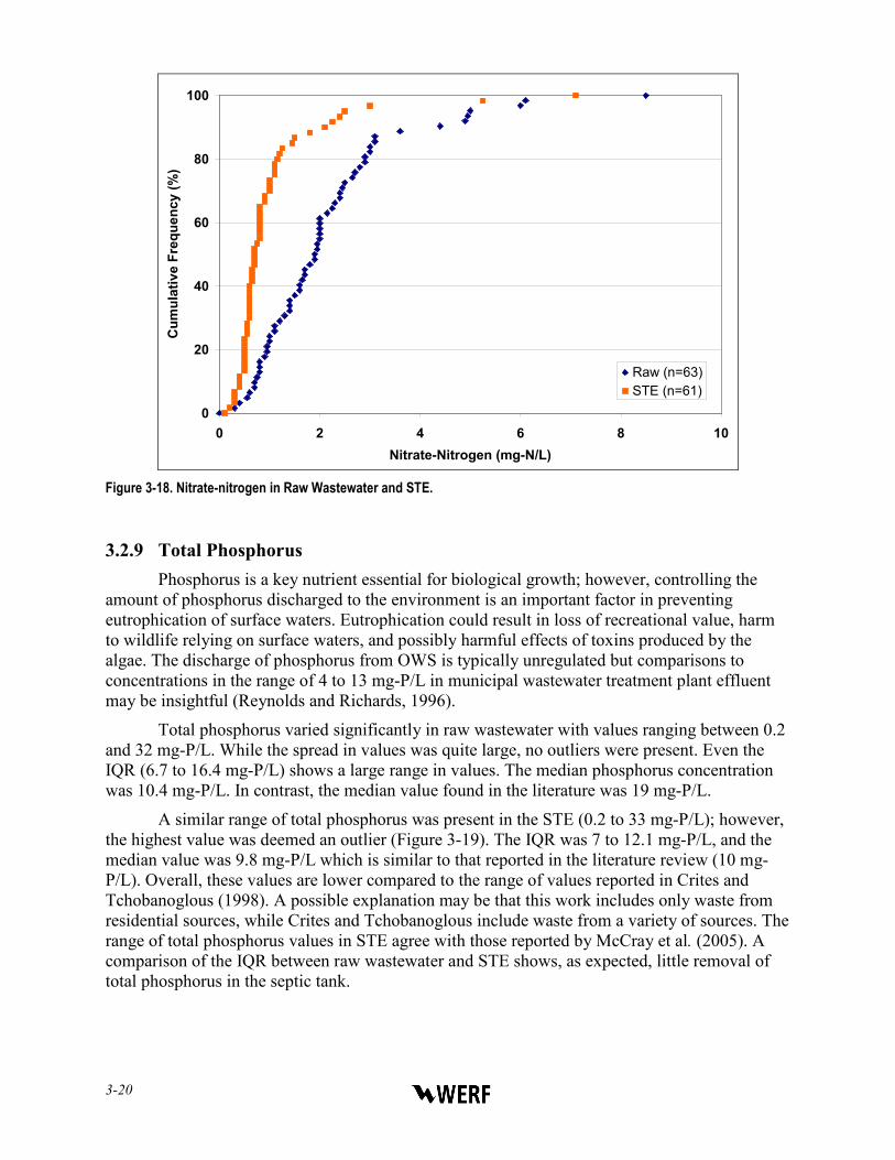
3-20
0
20
40
60
80
100
0 2 4 6 8 10Nitrate-Nitrogen (mg-N/L)
Cum
ulat
ive
Freq
uenc
y (%
)
Raw (n=63)STE (n=61)
Figure 3-18. Nitrate-nitrogen in Raw Wastewater and STE.
3.2.9 Total Phosphorus Phosphorus is a key nutrient essential for biological growth; however, controlling the
amount of phosphorus discharged to the environment is an important factor in preventing eutrophication of surface waters. Eutrophication could result in loss of recreational value, harm to wildlife relying on surface waters, and possibly harmful effects of toxins produced by the algae. The discharge of phosphorus from OWS is typically unregulated but comparisons to concentrations in the range of 4 to 13 mg-P/L in municipal wastewater treatment plant effluent may be insightful (Reynolds and Richards, 1996).
Total phosphorus varied significantly in raw wastewater with values ranging between 0.2 and 32 mg-P/L. While the spread in values was quite large, no outliers were present. Even the IQR (6.7 to 16.4 mg-P/L) shows a large range in values. The median phosphorus concentration was 10.4 mg-P/L. In contrast, the median value found in the literature was 19 mg-P/L.
A similar range of total phosphorus was present in the STE (0.2 to 33 mg-P/L); however, the highest value was deemed an outlier (Figure 3-19). The IQR was 7 to 12.1 mg-P/L, and the median value was 9.8 mg-P/L which is similar to that reported in the literature review (10 mg-P/L). Overall, these values are lower compared to the range of values reported in Crites and Tchobanoglous (1998). A possible explanation may be that this work includes only waste from residential sources, while Crites and Tchobanoglous include waste from a variety of sources. The range of total phosphorus values in STE agree with those reported by McCray et al. (2005). A comparison of the IQR between raw wastewater and STE shows, as expected, little removal of total phosphorus in the septic tank.

Influent Constituent Characteristics of the Modern Waste Stream from Single Sources 3-21
0
20
40
60
80
100
0 5 10 15 20 25 30 35Total Phosphorus (mg-P/L)
Cum
ulat
ive
Freq
uenc
y (%
)
Raw (n= 63)STE (n = 61)
Figure 3-19. Total Phosphorus in Raw Wastewater and STE.
3.2.10 Tier 1 Summary The results from the sampling event are summarized in Table 3-7. It is helpful to compare
the results of this study with the reported ranges in Onsite Wastewater Treatment Systems Manual (U.S. EPA, 2002) and Small and Decentralized Wastewater Management Systems (Crites and Tchobanoglous, 1998) because both are typically cited for median values and constituent ranges in raw wastewater and STE. The median values measured in this study of all constituents (except cBOD5) fall within the range reported in these two references. However, the constituent ranges of this work are significantly larger and are likely attributed to the limited number of previous studies on raw wastewater composition.

3-22
Table 3-7. Summary of Tier 1 Constituents from This Study and Previously Reported (in mg/L).
This Study U.S. EPA (2002)
Crites and Tchobanoglous
(1998) Median Range1 Lit. Review
Alkalinity (as CaCO3)
Raw 260 65 – 575 NR NR NR STE 411 172 – 862 NR NR 60 – 120
TS Raw 1,028 252 – 3,320 NR 500 – 880 350 – 1,200 STE 623 290 – 3,665 NR NR NR
TSS Raw 232 22 – 1,690 18 – 2,230 155 – 330 100 – 350 STE 61 28 – 192 22 – 276 50 – 100 40 – 140
cBOD5 Raw 420 112 – 1,101 30 – 1,147 155 – 286 110 – 400 STE 216 44 – 833 38 – 861 140 – 200 150 – 250
COD Raw 849 139 – 4,584 540 – 2,404 500 – 660 250 – 1,000 STE 389 201 – 944 157 – 1,931 NR 250 – 500
TOC Raw 184 35 – 738 NR NR 80 – 290 STE 105 50 – 243 NR 31 – 68 NR
DOC Raw 110 29 – 679 NR NR NR STE 66 22 – 140 NR NR NR
Total nitrogen Raw 60 9 – 240 44 – 189 26 – 75 20 – 85 STE 63 27 – 119 26 – 124 40 – 100 NR
TKN (as N) Raw 57 16 – 248 43 – 124 NR NR STE 60 33 – 171 27 – 94 19 – 53 50 – 90
Ammonium-nitrogen (as N)
Raw 14 2 – 94 9 – 154 4 – 13 12 – 50 STE 53 25 – 112 0 – 96 NR 30 – 50
Nitrate-nitrogen (as N)
Raw 1.9 BDL – 9 0.05 – 1.1 <1 0 STE 0.7 BDL – 7 0 – 10.3 0.01 – 0.16 NR
Total phosphorus
Raw 10.4 0.2 – 32 13 – 26 6 – 12 4 – 15 STE 9.8 0.2 – 33 3 – 40 7.2 – 17 12 – 20
1 All data included, outliers were not removed NR = not reported BDL = below detection limits
3.3 Tier 2: Oil and Grease and Microorganisms Tier 2 constituents included oil and grease and microorganisms providing addition
information on the waste stream composition. Approximately 50% of the samples collected were submitted for oil and grease analysis. Microbial analyses were conduced on all of the samples for fecal coliform bacteria and E. coli while coliphage was analyzed in 20% of the samples. While fecal coliform bacteria was a Tier 1 constituent, the findings are reported in Section 3.3.2 with E. coli and coliphage because of similar analytical techniques.
3.3.1 Oil and Grease Oil and grease typically originate from food wastes and other petroleum products. Oil and
grease is separated in the septic tank by floatation, but problems can arise if too much oil and grease enters the septic tank. For example, oil and grease does not break down easily resulting in an increased scum layer which in turn requires more frequent pumping. If oil and grease is not effectively removed in the septic tank, subsequent buildup in pipes or the soil treatment unit may lead to clogging.
Oil and grease in raw wastewater varied from 10 to 109 mg/L (Figure 3-20), which is slightly lower compared to the values reported in the literature review of 16 to 134 mg/L. This might be due to changing lifestyle habits (e.g. use of olive oil instead of lard for cooking), but
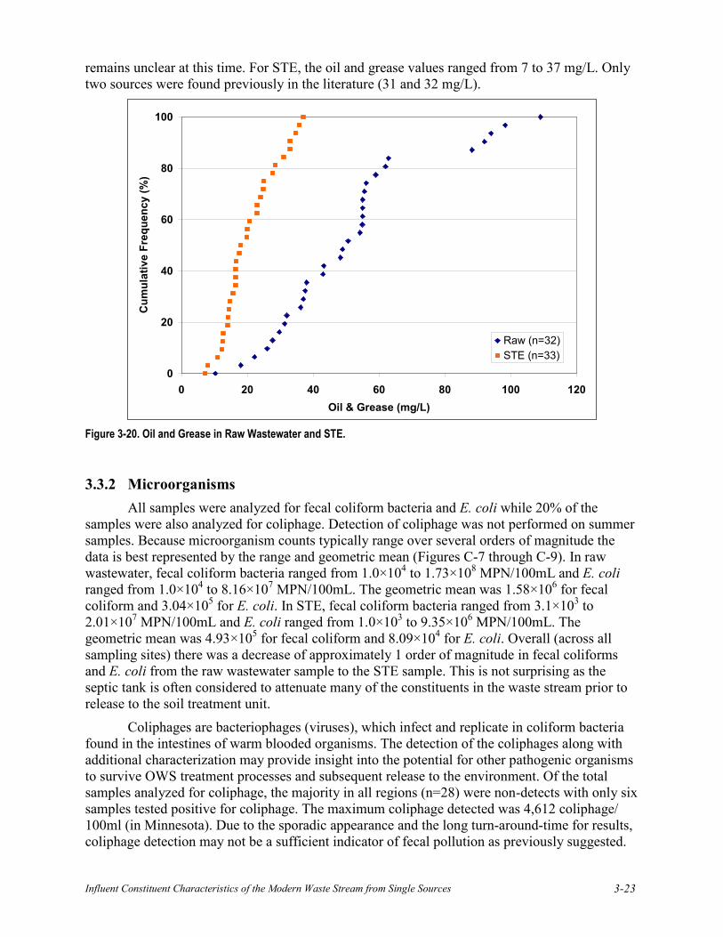
Influent Constituent Characteristics of the Modern Waste Stream from Single Sources 3-23
remains unclear at this time. For STE, the oil and grease values ranged from 7 to 37 mg/L. Only two sources were found previously in the literature (31 and 32 mg/L).
0
20
40
60
80
100
0 20 40 60 80 100 120Oil & Grease (mg/L)
Cum
ulat
ive
Freq
uenc
y (%
)
Raw (n=32)STE (n=33)
Figure 3-20. Oil and Grease in Raw Wastewater and STE.
3.3.2 Microorganisms All samples were analyzed for fecal coliform bacteria and E. coli while 20% of the
samples were also analyzed for coliphage. Detection of coliphage was not performed on summer samples. Because microorganism counts typically range over several orders of magnitude the data is best represented by the range and geometric mean (Figures C-7 through C-9). In raw wastewater, fecal coliform bacteria ranged from 1.0×10⁴ to 1.73×10⁸ MPN/100mL and E. coli ranged from 1.0×10⁴ to 8.16×10⁷ MPN/100mL. The geometric mean was 1.58×10⁶ for fecal coliform and 3.04×10⁵ for E. coli. In STE, fecal coliform bacteria ranged from 3.1×10³ to 2.01×10⁷ MPN/100mL and E. coli ranged from 1.0×10³ to 9.35×10⁶ MPN/100mL. The geometric mean was 4.93×10⁵ for fecal coliform and 8.09×10⁴ for E. coli. Overall (across all sampling sites) there was a decrease of approximately 1 order of magnitude in fecal coliforms and E. coli from the raw wastewater sample to the STE sample. This is not surprising as the septic tank is often considered to attenuate many of the constituents in the waste stream prior to release to the soil treatment unit.
Coliphages are bacteriophages (viruses), which infect and replicate in coliform bacteria found in the intestines of warm blooded organisms. The detection of the coliphages along with additional characterization may provide insight into the potential for other pathogenic organisms to survive OWS treatment processes and subsequent release to the environment. Of the total samples analyzed for coliphage, the majority in all regions (n=28) were non-detects with only six samples tested positive for coliphage. The maximum coliphage detected was 4,612 coliphage/ 100ml (in Minnesota). Due to the sporadic appearance and the long turn-around-time for results, coliphage detection may not be a sufficient indicator of fecal pollution as previously suggested.

3-24
Rather, it is likely that the detection of fecal coliphage in the waste stream is an indication of an episodic viral event with in the household. Thus, detection of coliphage may be important when investigating infectious disease outbreaks suspected to be caused by fecally contaminated drinking water.
Samples collected daily for a week and at four times during a single day were also examined for fecal coliforms and E. coli. The data indicated that fecal coliforms and E. coli numbers vary greatly from day to day, and are likely dependant on the activities of the household. The values observed in raw wastewater were more variable than in the STE for each region and is likely due to the attenuation of the waste stream in the septic tank. Although limited, a possible spike in fecal coliforms and E. coli numbers appears during the morning. Although it is unclear, it is also logical that there could be a spike at this time of day due to increased bathroom activities that generally occurs at this time.
Comparisons were examined within regions and sampling seasons, and across regions and sampling seasons. In general both fecal coliform and E. coli numbers were greatest in Minnesota and the least in Colorado (Figure 3-21). This phenomenon may be and indicator of water use or may make suggestions about household activities.
1.E+04
1.E+05
1.E+06
1.E+07
Colorado Florida MinnesotaSampling Region
MPN
/100
mL
Raw Fecal STE Fecal Raw E. coli STE E. coli
Figure 3-21. Regional Variations in Fecal Coliform Bacteria and E. coli.
In general, there appeared to be a lower concentration of fecal coliforms in the raw wastewater in the winter months in all regions (Figure 3-22). In Colorado the fall samples were slightly lower than in the winter, but the fall sampling was conducted in November during relatively cool temperatures. Furthermore, the fall and winter raw wastewater samples were nearly identical in fecal coliform enumeration (2.05 × 10⁵ and 2.64 × 10⁵ respectively), as were
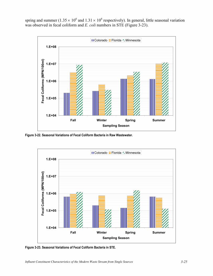
Influent Constituent Characteristics of the Modern Waste Stream from Single Sources 3-25
spring and summer (1.35 × 10⁶ and 1.31 × 10⁶ respectively). In general, little seasonal variation was observed in fecal coliform and E. coli numbers in STE (Figure 3-23).
1.E+04
1.E+05
1.E+06
1.E+07
1.E+08
Fall Winter Spring SummerSampling Season
Feca
l Col
iform
s (M
PN/1
00m
l)Colorado Florida Minnesota
Figure 3-22. Seasonal Variations of Fecal Coliform Bacteria in Raw Wastewater.
1.E+04
1.E+05
1.E+06
1.E+07
1.E+08
Fall Winter Spring SummerSampling Season
Feca
l Col
iform
s (M
PN/1
00m
l)
Colorado Florida Minnesota
Figure 3-23. Seasonal Variations of Fecal Coliform Bacteria in STE.
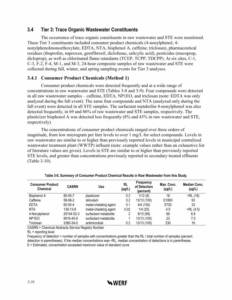
3-26
3.4 Tier 3: Trace Organic Wastewater Constituents The occurrence of trace organic constituents in raw wastewater and STE were monitored.
These Tier 3 constituents included consumer product chemicals (4-nonylphenol, 4-nonylphenolmonoethoxylate, EDTA, NTA, bisphenol A, caffeine, triclosan), pharmaceutical residues (ibuprofen, naproxen, gemfibrozil, diclofenac, salicylic acid), pesticides (mecoprop, dicloprop), as well as chlorinated flame retardants (TCEP, TCPP, TDCPP). At six sites, C-1, C-3, F-2, F-4, M-1, and M-3, 24-hour composite samples of raw wastewater and STE were collected during fall, winter, and spring sampling events for Tier 3 analyses.
3.4.1 Consumer Product Chemicals (Method 1) Consumer product chemicals were detected frequently and at a wide range of
concentrations in raw wastewater and STE (Tables 3-8 and 3-9). Four compounds were detected in all raw wastewater samples – caffeine, EDTA, NP1EO, and triclosan (note: EDTA was only analyzed during the fall event). The same four compounds and NTA (analyzed only during the fall event) were detected in all STE samples. The surfactant metabolite 4-nonylphenol was also detected frequently, in 69 and 86% of raw wastewater and STE samples, respectively. The plasticizer bisphenol A was detected less frequently (8% and 43% in raw wastewater and STE, respectively).
The concentrations of consumer product chemicals ranged over three orders of magnitude, from low microgram per liter levels to over 1 mg/L for select compounds. Levels in raw wastewater are similar to or higher than previously reported levels in municipal centralized wastewater treatment plant (WWTP) influent (note: example values rather than an exhaustive list of literature values are given). Levels in STE are similar to or higher than previously reported STE levels, and greater than concentrations previously reported in secondary treated effluents (Table 3-10).
Table 3-8. Summary of Consumer Product Chemical Results in Raw Wastewater from this Study.
Consumer Product Chemical CASRN Use RL
(μg/L) Frequency
of Detection (percent)
Max. Conc. (μg/L)
Median Conc. (μg/L)
Bisphenol A 80-05-7 plasticizer 0.2 1/12 (8) 18 <RL (18) Caffeine 58-08-2 stimulant 0.2 13/13 (100) E1800 93 EDTA 60-00-4 metal-chelating agent 0.1 4/4 (100) E720 33 NTA 139-13-9 metal-chelating agent 0.02 1/4 (25) 4.5 <RL (4.5) 4-Nonylphenol 25154-52-3 surfactant metabolite 2 9/13 (69) 66 6.8 NP1EO 9016-45-9 surfactant metabolite 1 13/13 (100) 23 7.5 Triclosan 3380-34-5 antimicrobial 0.2 13/13 (100) 230 19
CASRN = Chemical Abstracts Service Registry Number RL = reporting level Frequency of detection = number of samples with concentrations greater than the RL / total number of samples (percent detection in parentheses). If the median concentrations was <RL, median concentration of detections is in parentheses. E = Estimated, concentration exceeded maximum value of standard curve
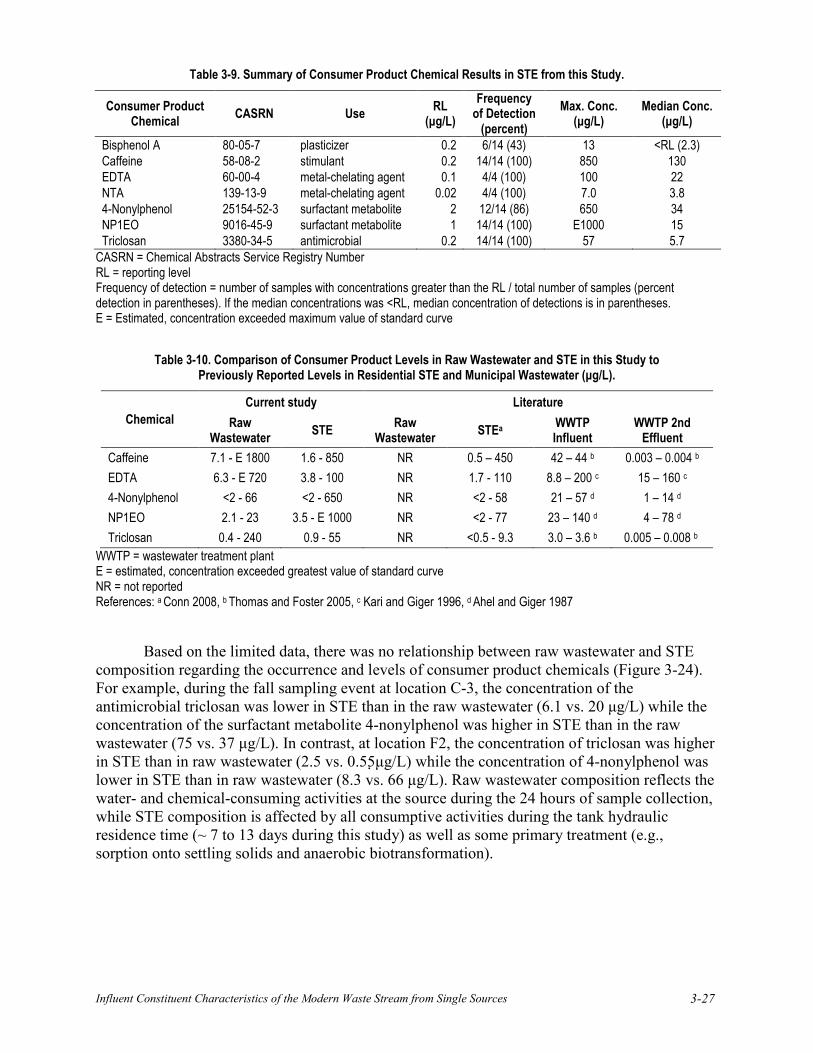
Influent Constituent Characteristics of the Modern Waste Stream from Single Sources 3-27
Table 3-9. Summary of Consumer Product Chemical Results in STE from this Study.
Consumer Product Chemical CASRN Use RL
(μg/L) Frequency
of Detection (percent)
Max. Conc. (μg/L)
Median Conc. (μg/L)
Bisphenol A 80-05-7 plasticizer 0.2 6/14 (43) 13 <RL (2.3) Caffeine 58-08-2 stimulant 0.2 14/14 (100) 850 130 EDTA 60-00-4 metal-chelating agent 0.1 4/4 (100) 100 22 NTA 139-13-9 metal-chelating agent 0.02 4/4 (100) 7.0 3.8 4-Nonylphenol 25154-52-3 surfactant metabolite 2 12/14 (86) 650 34 NP1EO 9016-45-9 surfactant metabolite 1 14/14 (100) E1000 15 Triclosan 3380-34-5 antimicrobial 0.2 14/14 (100) 57 5.7
CASRN = Chemical Abstracts Service Registry Number RL = reporting level Frequency of detection = number of samples with concentrations greater than the RL / total number of samples (percent detection in parentheses). If the median concentrations was <RL, median concentration of detections is in parentheses. E = Estimated, concentration exceeded maximum value of standard curve
Table 3-10. Comparison of Consumer Product Levels in Raw Wastewater and STE in this Study to Previously Reported Levels in Residential STE and Municipal Wastewater (μg/L).
Chemical Current study Literature
Raw Wastewater STE Raw
Wastewater STEa WWTP Influent
WWTP 2nd Effluent
Caffeine 7.1 - E 1800 1.6 - 850 NR 0.5 – 450 42 – 44 b 0.003 – 0.004 b
EDTA 6.3 - E 720 3.8 - 100 NR 1.7 - 110 8.8 – 200 c 15 – 160 c
4-Nonylphenol <2 - 66 <2 - 650 NR <2 - 58 21 – 57 d 1 – 14 d
NP1EO 2.1 - 23 3.5 - E 1000 NR <2 - 77 23 – 140 d 4 – 78 d
Triclosan 0.4 - 240 0.9 - 55 NR <0.5 - 9.3 3.0 – 3.6 b 0.005 – 0.008 b WWTP = wastewater treatment plant E = estimated, concentration exceeded greatest value of standard curve NR = not reported References: a Conn 2008, b Thomas and Foster 2005, c Kari and Giger 1996, d Ahel and Giger 1987
Based on the limited data, there was no relationship between raw wastewater and STE composition regarding the occurrence and levels of consumer product chemicals (Figure 3-24). For example, during the fall sampling event at location C-3, the concentration of the antimicrobial triclosan was lower in STE than in the raw wastewater (6.1 vs. 20 μg/L) while the concentration of the surfactant metabolite 4-nonylphenol was higher in STE than in the raw wastewater (75 vs. 37 μg/L). In contrast, at location F2, the concentration of triclosan was higher in STE than in raw wastewater (2.5 vs. 0.55μg/L) while the concentration of 4-nonylphenol was lower in STE than in raw wastewater (8.3 vs. 66 μg/L). Raw wastewater composition reflects the water- and chemical-consuming activities at the source during the 24 hours of sample collection, while STE composition is affected by all consumptive activities during the tank hydraulic residence time (~ 7 to 13 days during this study) as well as some primary treatment (e.g., sorption onto settling solids and anaerobic biotransformation).
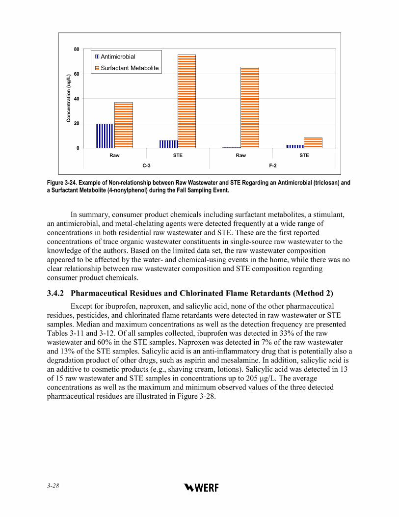
3-28
0
20
40
60
80
Raw STE Raw STE
C-3 F-2
Con
cent
ratio
n (u
g/L)
Antimicrobial
Surfactant Metabolite
Figure 3-24. Example of Non-relationship between Raw Wastewater and STE Regarding an Antimicrobial (triclosan) and a Surfactant Metabolite (4-nonylphenol) during the Fall Sampling Event.
In summary, consumer product chemicals including surfactant metabolites, a stimulant, an antimicrobial, and metal-chelating agents were detected frequently at a wide range of concentrations in both residential raw wastewater and STE. These are the first reported concentrations of trace organic wastewater constituents in single-source raw wastewater to the knowledge of the authors. Based on the limited data set, the raw wastewater composition appeared to be affected by the water- and chemical-using events in the home, while there was no clear relationship between raw wastewater composition and STE composition regarding consumer product chemicals.
3.4.2 Pharmaceutical Residues and Chlorinated Flame Retardants (Method 2) Except for ibuprofen, naproxen, and salicylic acid, none of the other pharmaceutical
residues, pesticides, and chlorinated flame retardants were detected in raw wastewater or STE samples. Median and maximum concentrations as well as the detection frequency are presented Tables 3-11 and 3-12. Of all samples collected, ibuprofen was detected in 33% of the raw wastewater and 60% in the STE samples. Naproxen was detected in 7% of the raw wastewater and 13% of the STE samples. Salicylic acid is an anti-inflammatory drug that is potentially also a degradation product of other drugs, such as aspirin and mesalamine. In addition, salicylic acid is an additive to cosmetic products (e.g., shaving cream, lotions). Salicylic acid was detected in 13 of 15 raw wastewater and STE samples in concentrations up to 205 μg/L. The average concentrations as well as the maximum and minimum observed values of the three detected pharmaceutical residues are illustrated in Figure 3-28.
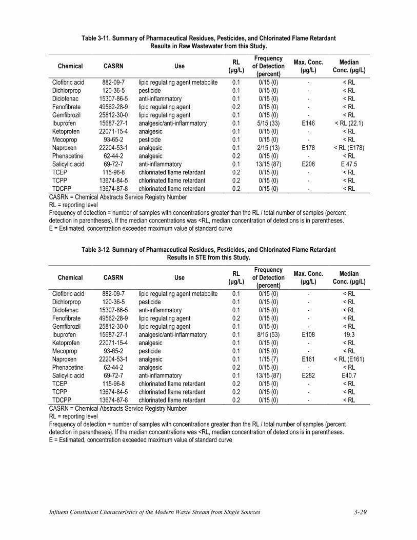
Influent Constituent Characteristics of the Modern Waste Stream from Single Sources 3-29
Table 3-11. Summary of Pharmaceutical Residues, Pesticides, and Chlorinated Flame Retardant Results in Raw Wastewater from this Study.
Chemical CASRN Use RL (μg/L)
Frequency of Detection
(percent) Max. Conc.
(μg/L) Median
Conc. (μg/L)
Clofibric acid 882-09-7 lipid regulating agent metabolite 0.1 0/15 (0) - < RL Dichlorprop 120-36-5 pesticide 0.1 0/15 (0) - < RL Diclofenac 15307-86-5 anti-inflammatory 0.1 0/15 (0) - < RL Fenofibrate 49562-28-9 lipid regulating agent 0.2 0/15 (0) - < RL Gemfibrozil 25812-30-0 lipid regulating agent 0.1 0/15 (0) - < RL Ibuprofen 15687-27-1 analgesic/anti-inflammatory 0.1 5/15 (33) E146 < RL (22.1) Ketoprofen 22071-15-4 analgesic 0.1 0/15 (0) - < RL Mecoprop 93-65-2 pesticide 0.1 0/15 (0) - < RL Naproxen 22204-53-1 analgesic 0.1 2/15 (13) E178 < RL (E178) Phenacetine 62-44-2 analgesic 0.2 0/15 (0) - < RL Salicylic acid 69-72-7 anti-inflammatory 0.1 13/15 (87) E208 E 47.5 TCEP 115-96-8 chlorinated flame retardant 0.2 0/15 (0) - < RL TCPP 13674-84-5 chlorinated flame retardant 0.2 0/15 (0) - < RL TDCPP 13674-87-8 chlorinated flame retardant 0.2 0/15 (0) - < RL
CASRN = Chemical Abstracts Service Registry Number RL = reporting level Frequency of detection = number of samples with concentrations greater than the RL / total number of samples (percent detection in parentheses). If the median concentrations was <RL, median concentration of detections is in parentheses. E = Estimated, concentration exceeded maximum value of standard curve
Table 3-12. Summary of Pharmaceutical Residues, Pesticides, and Chlorinated Flame Retardant Results in STE from this Study.
Chemical CASRN Use RL (μg/L)
Frequency of Detection
(percent) Max. Conc.
(μg/L) Median
Conc. (μg/L)
Clofibric acid 882-09-7 lipid regulating agent metabolite 0.1 0/15 (0) - < RL Dichlorprop 120-36-5 pesticide 0.1 0/15 (0) - < RL Diclofenac 15307-86-5 anti-inflammatory 0.1 0/15 (0) - < RL Fenofibrate 49562-28-9 lipid regulating agent 0.2 0/15 (0) - < RL Gemfibrozil 25812-30-0 lipid regulating agent 0.1 0/15 (0) - < RL Ibuprofen 15687-27-1 analgesic/anti-inflammatory 0.1 8/15 (53) E108 19.3 Ketoprofen 22071-15-4 analgesic 0.1 0/15 (0) - < RL Mecoprop 93-65-2 pesticide 0.1 0/15 (0) - < RL Naproxen 22204-53-1 analgesic 0.1 1/15 (7) E161 < RL (E161) Phenacetine 62-44-2 analgesic 0.2 0/15 (0) - < RL Salicylic acid 69-72-7 anti-inflammatory 0.1 13/15 (87) E282 E40.7 TCEP 115-96-8 chlorinated flame retardant 0.2 0/15 (0) - < RL TCPP 13674-84-5 chlorinated flame retardant 0.2 0/15 (0) - < RL TDCPP 13674-87-8 chlorinated flame retardant 0.2 0/15 (0) - < RL
CASRN = Chemical Abstracts Service Registry Number RL = reporting level Frequency of detection = number of samples with concentrations greater than the RL / total number of samples (percent detection in parentheses). If the median concentrations was <RL, median concentration of detections is in parentheses. E = Estimated, concentration exceeded maximum value of standard curve

3-30
0
20
40
60
80
100
120
140
160
180
Raw Wastewater STE
Con
cent
ratio
n (u
g/L)
Salicylic AcidIbuprofenNaproxen
Figure 3-28. Average Concentration of Ibuprofen, Naproxen, and Salicylic Acid Observed in Raw Wastewater and STE Samples for all Sampling Events.
Most of the targeted pharmaceutical residues did not occur in any of the samples collected from raw wastewater or STE during this study. It is noteworthy, that the occurrence of these compounds is site specific and directly related to the consumption of human pharmaceuticals. Composite sampling over 24-hours or over several days might still not be sufficient to capture sporadic discharge events. In contrast, target pharmaceutical compounds are more prevalent in centralized municipal wastewater treatment plants treating wastewater from a larger number of households and other wastewater sources. A summary of occurrence levels in samples collected from residential OWS, STE, and WWTP in- and effluents are summarized in Table 3-13.
Limited data is published in the peer-reviewed literature on the occurrence as well as the fate and transport of pharmaceutical residues in OWS. Carrara et al. (2008) studied the occurrence of pharmaceutical residues in STE at two campsites in Canada with 200-2000 occupants (Table 3-13). Similar to the current study, painkillers were especially detected, although at significantly lower concentrations than observed in this study. Due to the higher occupancy at the campground, more dilution of the wastewater can be expected in the STE.
As discussed for the consumer chemical products, no correlation between the occurrence of pharmaceutical residues in the raw wastewater compared STE was observed. Results for ibuprofen and salicylic acid for two sampling events are illustrated in Figure 3-29. The composition in the raw wastewater as well as the STE varied not only between different sampling events, but also for different compounds during the same event. While not only the consumption of pharmaceutical residues, especially non-prescription drugs, may vary from day to day, also the conditions (e.g., residence time, temperature, load of organic compounds) during treatment in the septic tank at different sites can vary significantly. These findings suggest that the occurrence of pharmaceutical residues in single residential sources will be highly variable.

Influent Constituent Characteristics of the Modern Waste Stream from Single Sources 3-31
Table 3-13. Comparison of Pharmaceutical Residue Levels in Raw Wastewater and STE in this Study to Previously Reported Levels in Residential STE and Municipal Wastewater (μg/L).
Chemical This Study Literature
Raw Wastewater STE Raw
Wastewater STE WWTP 2nd Effluent
Clofibric acid < 0.1 < 0.1 NR < RLa < RL - 0.03b Dichlorprop < 0.1 < 0.1 NR - - Diclofenac < 0.1 < 0.1 NR < RLa < RL - 3.46b Fenofibrate < 0.2 < 0.2 NR < RLa - Gemfibrozil < 0.1 < 0.1 NR 0.015 - 0.62a < RL - 1.3b Ibuprofen < 0.1 - E146 < 0.1 - E108 NR 2.4 - 6.8a < RL - 24.6b Ketoprofen < 0.1 < 0.1 NR < RLa < RL - 0.045b Mecoprop < 0.1 < 0.1 NR - - Naproxen < 0.1 - E179 < 0.1 - E151 NR 0.009 - 0.3a < RL - 33.9b Phenacetine < 0.2 < 0.2 NR - - Salicylic acid < 0.1 - E209 < 0.1 - E208 NR < RL - 0.48a < RL - 4.8b TCEP < 0.2 < 0.2 NR - - TCPP < 0.2 < 0.2 NR - - TDCPP < 0.2 < 0.2 NR - -
WWTP = wastewater treatment plant E = estimated, concentration exceeded greatest value of standard curve NR = not reported References: a Carrara et al. 2008, b Snyder et al. 2008
0
5
10
15
20
25
30
35
40
Raw Wastewater STE Raw Wastewater STE
Winter Spring
Con
cent
ratio
n (u
g/L)
Salicylic Acid
Ibuprofen
Site M-1
Figure 3-29. Occurrence of Ibuprofen and Salicylic Acid in Raw Wastewater and STE Samples.
Site F-2
0
20
40
60
80
100
120
140
160
RawWastewater
STE RawWastewater
STE RawWastewater
STE
Fall Winter Spring
Con
cent
ratio
n (u
g/L)
Salicylic Acid
Ibuprofen

3-32
Influent Constituent Characteristics of the Modern Waste Stream from Single Sources 4-1
CHAPTER 4.0
DISCUSSION
The monitoring framework for this study was designed to have broad applicability by encompassing different regional locations, seasons, number of occupants, and age of the occupants. The results of the combined data were presented in Chapter 3.0 with additional supporting information presented in Appendices B and C. This data is especially useful for aiding decision making during OWS design and/or assessment of environmental and public health impacts. For example, if an OWS is being designed to remove 60% of the total nitrogen from a residential source, then values of expected average total nitrogen concentrations in either raw wastewater or STE can be chosen from the associated CFDs. In this scenario, if a 50th percentile value is selected from the CFD (e.g., 59 mg-N/L in STE), the designer can assume that half of the homes in the US will have average total nitrogen concentrations less than or equal to 59 mg-N/L and plan for final concentrations of approximately 24 mg-N/L. If the same system is to be installed in a nitrogen sensitive environment, the designer may select a more conservative value such as the 90th percentile value (e.g., ~89 mg-N/L) which suggests that only 10% of the households are expected to have higher average total nitrogen concentrations and plan for a final concentration of ~36 mg-N/L. Alternatively, if the final concentration can not exceed a specific value (e.g., 20 mg-N/L) the level of nitrogen removal can be estimated (i.e., 66% reduction of the 50th percentile estimate or 76% reduction of the 90th percentile estimate would be required).
Differences in waste stream composition attributed to regional location, season, number of occupants, and the age of the occupants could also be helpful for decision makers. If differences in these parameters can be defined (which may or may not be statistically significant), then the user can select the best possible available data applicable to a very specific decision. In this scenario, a designer may wish to select data specific to occupants over the age of 65 in Florida. For example, in the over 65 in Florida scenario, comparison of the 75th percentile value of expected cBOD5 concentration in raw wastewater in Florida (615 mg/L) can be compared to 75th percentile value of expected cBOD5 concentration in raw wastewater in occupants over 65 (686 mg/L) (see Table B-10). In the absence of this type of detail, a decision maker has been forced to use reported average or median values with some random level of contingency (e.g., average raw cBOD5 value of 343 mg/L ± 69 mg/L as reported in the Phase 1 Literature Review, Lowe et al., 2007). In this example the average literature value is nearly half what was actually observed. An understanding of this level of detail in the data can be especially useful for input into models enabling assessment of various “what if” scenarios while also providing insight into the uncertainty of the output result based on variations in the selected input values.
Correlations between various constituents or between raw wastewater and STE are also useful tools. In an ideal case, an easily obtained parameter value could be used to approximate a difficult to obtain parameter value. For example, if the raw wastewater cBOD5 concentration can be approximated from COD concentrations in STE, significant time and money could be saved for individual projects. In this scenario and in the absence of additional data, sufficient insight or understanding may be gained through the use of easily and economically obtained information.
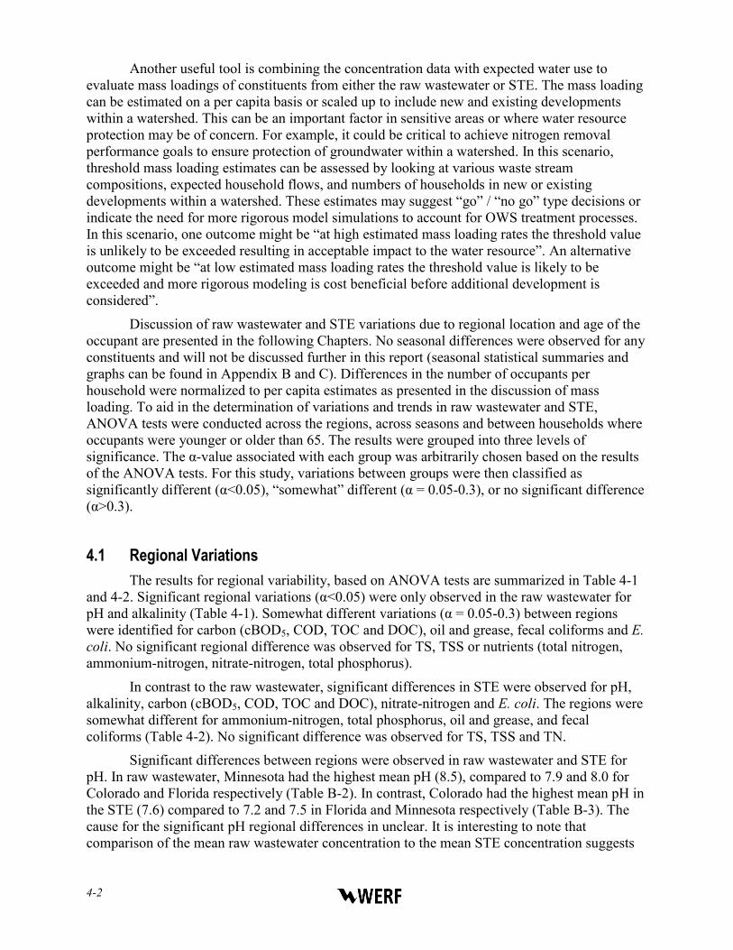
4-2
Another useful tool is combining the concentration data with expected water use to evaluate mass loadings of constituents from either the raw wastewater or STE. The mass loading can be estimated on a per capita basis or scaled up to include new and existing developments within a watershed. This can be an important factor in sensitive areas or where water resource protection may be of concern. For example, it could be critical to achieve nitrogen removal performance goals to ensure protection of groundwater within a watershed. In this scenario, threshold mass loading estimates can be assessed by looking at various waste stream compositions, expected household flows, and numbers of households in new or existing developments within a watershed. These estimates may suggest “go” / “no go” type decisions or indicate the need for more rigorous model simulations to account for OWS treatment processes. In this scenario, one outcome might be “at high estimated mass loading rates the threshold value is unlikely to be exceeded resulting in acceptable impact to the water resource”. An alternative outcome might be “at low estimated mass loading rates the threshold value is likely to be exceeded and more rigorous modeling is cost beneficial before additional development is considered”.
Discussion of raw wastewater and STE variations due to regional location and age of the occupant are presented in the following Chapters. No seasonal differences were observed for any constituents and will not be discussed further in this report (seasonal statistical summaries and graphs can be found in Appendix B and C). Differences in the number of occupants per household were normalized to per capita estimates as presented in the discussion of mass loading. To aid in the determination of variations and trends in raw wastewater and STE, ANOVA tests were conducted across the regions, across seasons and between households where occupants were younger or older than 65. The results were grouped into three levels of significance. The α-value associated with each group was arbitrarily chosen based on the results of the ANOVA tests. For this study, variations between groups were then classified as significantly different (α<0.05), “somewhat” different (α = 0.05-0.3), or no significant difference (α>0.3).
4.1 Regional Variations The results for regional variability, based on ANOVA tests are summarized in Table 4-1
and 4-2. Significant regional variations (α<0.05) were only observed in the raw wastewater for pH and alkalinity (Table 4-1). Somewhat different variations (α = 0.05-0.3) between regions were identified for carbon (cBOD5, COD, TOC and DOC), oil and grease, fecal coliforms and E. coli. No significant regional difference was observed for TS, TSS or nutrients (total nitrogen, ammonium-nitrogen, nitrate-nitrogen, total phosphorus).
In contrast to the raw wastewater, significant differences in STE were observed for pH, alkalinity, carbon (cBOD5, COD, TOC and DOC), nitrate-nitrogen and E. coli. The regions were somewhat different for ammonium-nitrogen, total phosphorus, oil and grease, and fecal coliforms (Table 4-2). No significant difference was observed for TS, TSS and TN.
Significant differences between regions were observed in raw wastewater and STE for pH. In raw wastewater, Minnesota had the highest mean pH (8.5), compared to 7.9 and 8.0 for Colorado and Florida respectively (Table B-2). In contrast, Colorado had the highest mean pH in the STE (7.6) compared to 7.2 and 7.5 in Florida and Minnesota respectively (Table B-3). The cause for the significant pH regional differences in unclear. It is interesting to note that comparison of the mean raw wastewater concentration to the mean STE concentration suggests
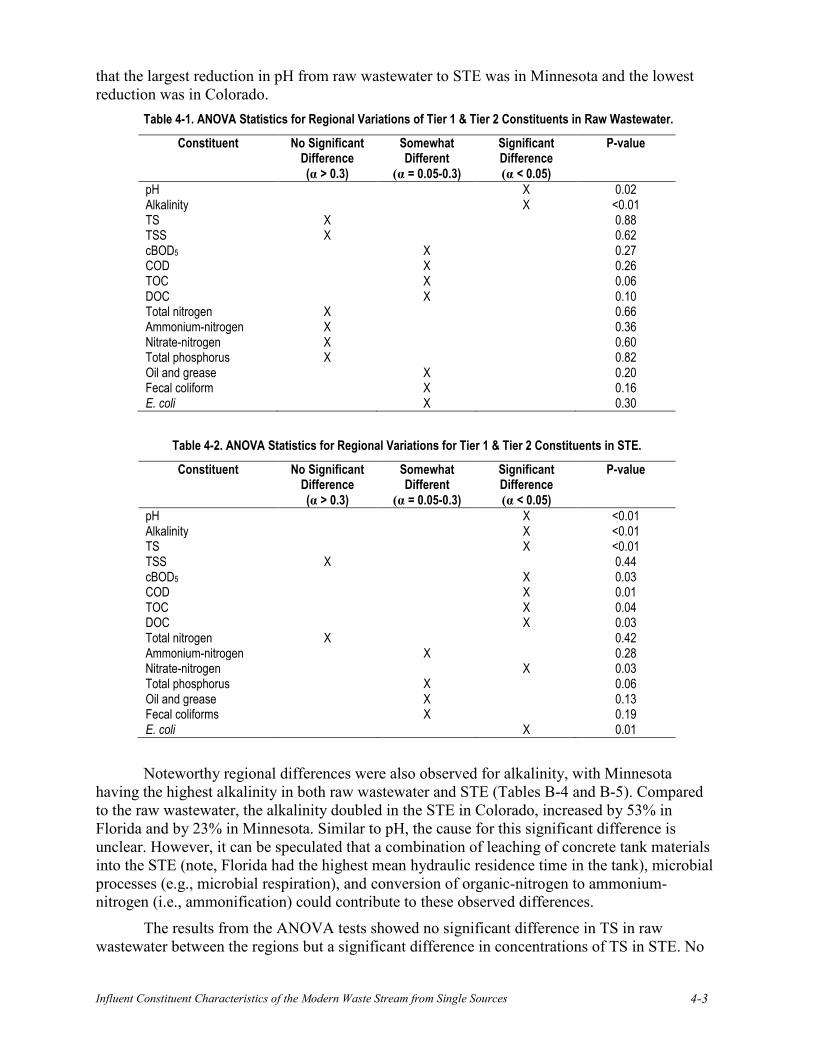
Influent Constituent Characteristics of the Modern Waste Stream from Single Sources 4-3
that the largest reduction in pH from raw wastewater to STE was in Minnesota and the lowest reduction was in Colorado.
Table 4-1. ANOVA Statistics for Regional Variations of Tier 1 & Tier 2 Constituents in Raw Wastewater.
Constituent No Significant Difference (α > 0.3)
Somewhat Different
(α = 0.05-0.3)
Significant Difference (α < 0.05)
P-value
pH X 0.02 Alkalinity X <0.01 TS X 0.88 TSS X 0.62 cBOD5 X 0.27 COD X 0.26 TOC X 0.06 DOC X 0.10 Total nitrogen X 0.66 Ammonium-nitrogen X 0.36 Nitrate-nitrogen X 0.60 Total phosphorus X 0.82 Oil and grease X 0.20 Fecal coliform X 0.16 E. coli X 0.30
Table 4-2. ANOVA Statistics for Regional Variations for Tier 1 & Tier 2 Constituents in STE.
Constituent No Significant Difference (α > 0.3)
Somewhat Different
(α = 0.05-0.3)
Significant Difference (α < 0.05)
P-value
pH X <0.01 Alkalinity X <0.01 TS X <0.01 TSS X 0.44 cBOD5 X 0.03 COD X 0.01 TOC X 0.04 DOC X 0.03 Total nitrogen X 0.42 Ammonium-nitrogen X 0.28 Nitrate-nitrogen X 0.03 Total phosphorus X 0.06 Oil and grease X 0.13 Fecal coliforms X 0.19 E. coli X 0.01
Noteworthy regional differences were also observed for alkalinity, with Minnesota having the highest alkalinity in both raw wastewater and STE (Tables B-4 and B-5). Compared to the raw wastewater, the alkalinity doubled in the STE in Colorado, increased by 53% in Florida and by 23% in Minnesota. Similar to pH, the cause for this significant difference is unclear. However, it can be speculated that a combination of leaching of concrete tank materials into the STE (note, Florida had the highest mean hydraulic residence time in the tank), microbial processes (e.g., microbial respiration), and conversion of organic-nitrogen to ammonium-nitrogen (i.e., ammonification) could contribute to these observed differences.
The results from the ANOVA tests showed no significant difference in TS in raw wastewater between the regions but a significant difference in concentrations of TS in STE. No
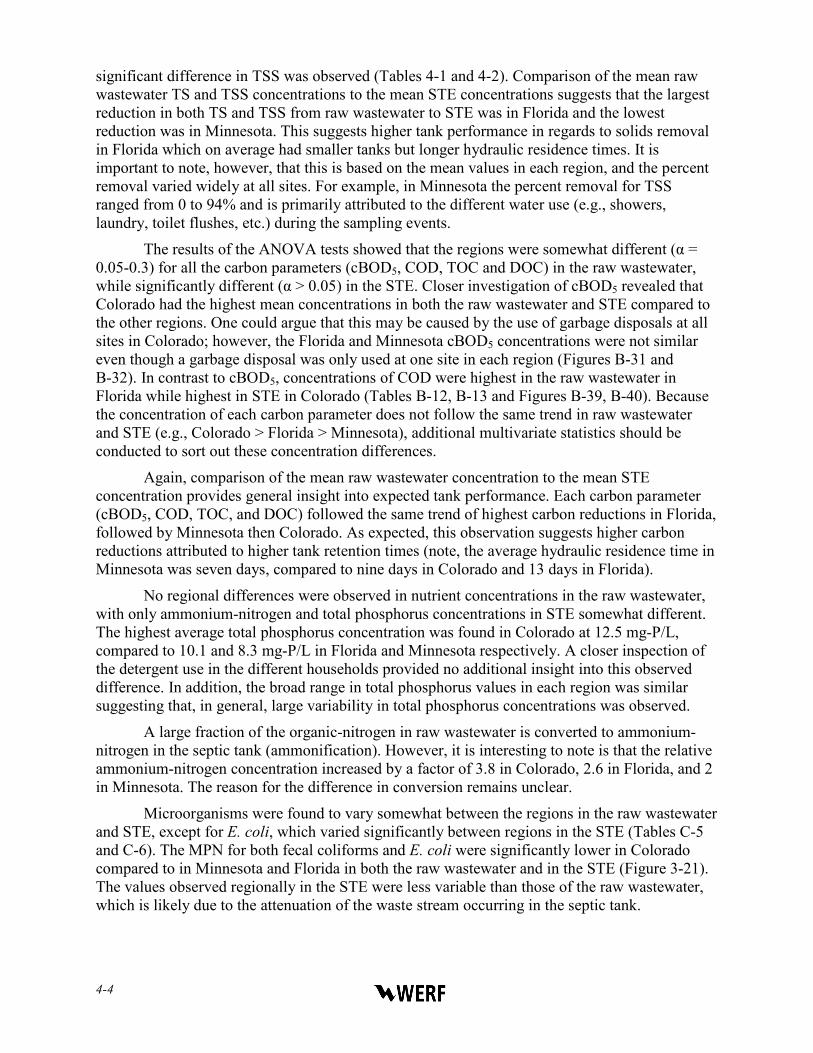
4-4
significant difference in TSS was observed (Tables 4-1 and 4-2). Comparison of the mean raw wastewater TS and TSS concentrations to the mean STE concentrations suggests that the largest reduction in both TS and TSS from raw wastewater to STE was in Florida and the lowest reduction was in Minnesota. This suggests higher tank performance in regards to solids removal in Florida which on average had smaller tanks but longer hydraulic residence times. It is important to note, however, that this is based on the mean values in each region, and the percent removal varied widely at all sites. For example, in Minnesota the percent removal for TSS ranged from 0 to 94% and is primarily attributed to the different water use (e.g., showers, laundry, toilet flushes, etc.) during the sampling events.
The results of the ANOVA tests showed that the regions were somewhat different (α = 0.05-0.3) for all the carbon parameters (cBOD5, COD, TOC and DOC) in the raw wastewater, while significantly different (α > 0.05) in the STE. Closer investigation of cBOD5 revealed that Colorado had the highest mean concentrations in both the raw wastewater and STE compared to the other regions. One could argue that this may be caused by the use of garbage disposals at all sites in Colorado; however, the Florida and Minnesota cBOD5 concentrations were not similar even though a garbage disposal was only used at one site in each region (Figures B-31 and B-32). In contrast to cBOD5, concentrations of COD were highest in the raw wastewater in Florida while highest in STE in Colorado (Tables B-12, B-13 and Figures B-39, B-40). Because the concentration of each carbon parameter does not follow the same trend in raw wastewater and STE (e.g., Colorado > Florida > Minnesota), additional multivariate statistics should be conducted to sort out these concentration differences.
Again, comparison of the mean raw wastewater concentration to the mean STE concentration provides general insight into expected tank performance. Each carbon parameter (cBOD5, COD, TOC, and DOC) followed the same trend of highest carbon reductions in Florida, followed by Minnesota then Colorado. As expected, this observation suggests higher carbon reductions attributed to higher tank retention times (note, the average hydraulic residence time in Minnesota was seven days, compared to nine days in Colorado and 13 days in Florida).
No regional differences were observed in nutrient concentrations in the raw wastewater, with only ammonium-nitrogen and total phosphorus concentrations in STE somewhat different. The highest average total phosphorus concentration was found in Colorado at 12.5 mg-P/L, compared to 10.1 and 8.3 mg-P/L in Florida and Minnesota respectively. A closer inspection of the detergent use in the different households provided no additional insight into this observed difference. In addition, the broad range in total phosphorus values in each region was similar suggesting that, in general, large variability in total phosphorus concentrations was observed.
A large fraction of the organic-nitrogen in raw wastewater is converted to ammonium-nitrogen in the septic tank (ammonification). However, it is interesting to note is that the relative ammonium-nitrogen concentration increased by a factor of 3.8 in Colorado, 2.6 in Florida, and 2 in Minnesota. The reason for the difference in conversion remains unclear.
Microorganisms were found to vary somewhat between the regions in the raw wastewater and STE, except for E. coli, which varied significantly between regions in the STE (Tables C-5 and C-6). The MPN for both fecal coliforms and E. coli were significantly lower in Colorado compared to in Minnesota and Florida in both the raw wastewater and in the STE (Figure 3-21). The values observed regionally in the STE were less variable than those of the raw wastewater, which is likely due to the attenuation of the waste stream occurring in the septic tank.

Influent Constituent Characteristics of the Modern Waste Stream from Single Sources 4-5
It was initially hypothesized that the concentrations of oil and grease would vary greatly between regions due to lifestyle habits. However, the raw wastewater across regions was observed to be only somewhat different, Colorado (54 mg/L mean), Florida (55 mg/L mean) and Minnesota (35 mg/L mean) (Table C-1). Again, similar to carbon and nutrient concentrations, significant regional differences were observed in STE. Florida has the greatest removal in the tank by a factor of 2.75 (ratio of mean raw wastewater concentration to mean STE concentration), compared to a factor of 2.2 in both Colorado and Minnesota. The high removal in Florida may be attributed to the higher hydraulic residence time in the septic tank.
In summary, although the contributing factors are not clear, regional differences were observed between raw wastewater and STE concentrations. As illustrated in Tables 4-1 and 4-2, while there did not appear to be significant differences in the composition of the raw wastewater attributed to region, there were significant differences in the STE from these same raw wastewater sources. This suggests that STE from relatively similar sources may indeed vary significantly. Since it can be assumed that the processes and mechanisms responsible for these differences are the same in each region, other factors such as temperature, tank size, hydraulic residence time in the septic tank, etc., should be considered. In addition, the complex interactions between various potential factors (e.g., tank size) and processes (e.g., microbial respiration) should be considered. While the number of data points obtained in this study may limit the ability of statistical methods to identify subtle differences attributed to these factors and processes, additional multivariate statistics should be conducted. For example specific statistical tests need to be conducted to ascertain what role leaching of concrete tank materials and the subsequent increase in observed alkalinity in STE may play relative to the anaerobic ammonification of organic-nitrogen and the generation of alkalinity, relative to slight differences observed in septic tank reductions of cBOD5 and pH.
4.2 Occupant Age Variations The results for variability attributed to the age of the occupants, based on ANOVA tests
are summarized in Tables 4-3 and 4-4. Significant variations (α<0.05) were only observed in the raw wastewater for pH, alkalinity, and TS between households where the occupants were older or younger than 65 (Table 4-3). In contrast, significant differences were observed for alkalinity, TS, carbon, and nutrient constituents in STE (Table 4-4). The raw wastewater was found to be somewhat different (α = 0.05-0.3) for cBOD5, nutrients, oil and grease, and E. coli, while STE was only somewhat different for TSS. No significant difference (α>0.3) was observed for TSS, COD, TOC, DOC, and fecal coliform bacteria in raw wastewater and for pH, oil and grease, fecal coliform and E. coli in STE.
The average pH level was found to be significantly higher (8.4) in the raw wastewater in households where the occupants were older than 65, compared to in households with younger residents (7.9). In contrast, no difference was observed in the STE (7.4), suggesting that the tank equalizes the waste stream. The average alkalinity level was found to be significantly higher in households with older residents compared to in the households with younger residents for both raw wastewater (330 mg-CaCO3/L vs. 244 mg-CaCO3/L) and STE (490 mg-CaCO3/L vs. 364 mg-CaCO3/L). It is interesting to note that the ratio between alkalinity concentrations for occupants over 65 to occupants under 65 was 1.35 for both raw wastewater and STE.

4-6
Table 4-3. ANOVA Statistics for Occupant Age Variations of Tier 1 and Tier 2 Constituents in Raw Wastewater.
Constituent No Significant Difference (α > 0.3)
Somewhat Different
(α = 0.05-0.3)
Significant Difference (α < 0.05)
P-value
pH X <0.01 Alkalinity X 0.02 TS X 0.02 TSS X 0.47 cBOD5 X 0.06 COD X 0.59 TOC X 0.72 DOC X 0.56 Total nitrogen X 0.11 Ammonium-nitrogen X 0.11 Nitrate-nitrogen X 0.12 Total phosphorus X 0.11 Oil and grease X 0.11 Fecal coliform X 0.82 E. coli X 0.17 Table 4-4. ANOVA Statistics for Occupant Age Variations of Tier 1 and Tier 2 Constituents in STE.
Constituent No Significant Difference (α > 0.3)
Somewhat Different
(α = 0.05-0.3)
Significant Difference (α < 0.05)
P-value
pH X 0.44 Alkalinity X <0.01 TS X <0.01 TSS X 0.17 cBOD5 X <0.01 COD X <0.01 TOC X 0.03 DOC X 0.01 Total nitrogen X <0.01 Ammonium-nitrogen X <0.01 Nitrate-nitrogen X 0.01 Total phosphorus X <0.01 Oil and grease X 0.95 Fecal coliform X 0.89 E. coli X 0.41
The average values for cBOD5 in raw wastewater were found to vary somewhat in households with occupants older than 65 compared to occupants younger than 65 (508 mg/L compared to 405 mg/L, respectively) (Table B-10). The age of the occupants did not suggest a significant difference in the raw wastewater for the other carbon parameters (COD, TOC, DOC). Although the age of the occupants were not significantly different for average COD values, it is interesting to note that the households with the younger occupants had a greater range of COD values (e.g., higher variability in the COD concentrations).
In contrast, the age of the occupants appeared to have a significant impact on the concentrations of cBOD5, COD, TOC, and DOC in the STE (Table B-11), with higher average concentrations for each parameter when occupants were older than 65. It remains unclear why age appeared to have little to no impact on the raw wastewater, while a significant impact on the STE. However, interesting observations were noted. The ratio of the parameter concentration in

Influent Constituent Characteristics of the Modern Waste Stream from Single Sources 4-7
STE for households with occupants over 65 compared to the parameter concentration in STE for households with occupants under 65 varied by carbon constituent (1.55 for cBOD5, 1.39 for COD, 1.24 for TOC, and 1.32 for DOC). This suggests the type of carbon and the distribution of the carbon fractions are different based on occupant age. Further analysis would be required to identify the various carbon fractions. It is also interesting to note the differences in tank removals. For each parameter, higher reductions (difference between raw wastewater concentration and STE concentration) were observed in households with occupants under 65. Specifically, the percent removal observed for cBOD5 was 36% (>65) vs. 48% (<65), for COD was 47% (>65) vs. 58% (<65), and for TOC and DOC was 33-35% (>65) vs. 50-55% (<65). The difference in water use may explain the variability seen in carbon constituents, where water use by older residents in this study averaged 297 L/capita/d (78.5 gpcd), compared to younger residents that averaged 148 L/capita/d (39.1 gpcd) although the hydraulic residence times in the septic tank were comparable (Figure 4-1, average 11 days for occupants under 65 and eight days for occupants under 65). Additionally, the type of water use may attribute to the difference with less shower and laundry use and higher kitchen and toilet use in the households with older occupants.
0
20
40
60
80
100
0 10 20 30 40 50 60Hydraulic Residence Time (d)
Cum
ulat
ive
Freq
uenc
y (%
)
65> 65<
Figure 4-1. Hydraulic Residence Time in the Septic Tank by Age of Occupant.
Similar to carbon constituents, the nutrients were found to only vary somewhat in the raw wastewater, but differ significantly in STE. For each constituent (total nitrogen, ammonium-nitrogen, nitrate-nitrogen, and total phosphorus), the strength of the waste was higher in households where the occupants were older than 65. This is supported by higher toilet and kitchen use (i.e. dishwasher, disposal, etc.) in households with older occupants. Table 4-5 summarizes the ratio of average nutrient concentration in STE for households with older occupants compared to households with younger occupants.

4-8
Table 4-5. Ratio of Average Concentrations of Households with Occupants >65 to Households with Occupants <65.
Nutrient Raw Wastewater STE
Total nitrogen 1.28 1.28
Ammonium-nitrogen 1.46 1.29
Nitrate-nitrogen 1.32 1.88
Total phosphorus 1.29 1.63
In summary, differences were observed between raw wastewater and STE concentrations attributed to the age of the occupants (over 65 vs. under 65) although the contributing factors remain unclear. Similar to regional variations, Tables 4-3 and 4-4, suggest that while there did not appear to be significant differences in the composition of the raw wastewater attributed to age, there were significant differences in the STE from these same raw wastewater sources. This suggests that STE from relatively similar sources may indeed vary significantly and additional multivariate statistics should be conducted.
4.3 Weekly and Daily Variations To assess expected variations in the wastewater on a weekly basis, raw wastewater and
STE samples were collected every day for a seven-day period at one site in each region (C-5, F-2, and M-2). The samples were analyzed for all Tier 1 constituents including fecal coliforms and E. coli. Each week long sampling event started on a Monday to allow comparison of the results between the regions. At one site (F-2) the occupants were over 65 while at the remaining two sites (C-5 and M-2), the occupants were under age 65. However, due to the limited number of sites monitored, regional and age trends can not be assessed. During the development of the raw wastewater sampling method, the STE was analyzed for several days after the use of the macerating pump to ensure that its use did not impact the STE. At the Colorado site (C-5), STE was collected for two additional days to further investigate if the use of the macerating pump showed any impact on the characteristics of the STE.
4.3.1 Weekly Variations Weekly variations were observed at all three sampling sites in the raw wastewater for all
constituents, while little variability was present in the STE (Appendix D). These results confirm that the septic tank equalizes not only the flow, but also the wastewater composition dampening the large “spikes” observed in raw wastewater. The extended STE sampling at site C-5 also showed that the macerating pump did not appear to impact the characteristics of the STE. The hydraulic residence time in the septic tank at C-5 (based on the water use each day) varied from 1.4 to 4 days during the weeklong sampling event; hence, the sampling event was greater than the hydraulic residence time and any changes in composition would be captured.
The total nitrogen results from the weekly sampling events at each site are illustrated in Figures 4-2 through 4-4. The graphs clearly show the variations in the raw wastewater over the course of the week, while little change was observed in the STE. It is interesting to note that there appears to be a strong inverse relationship with total nitrogen concentrations in the raw wastewater and water use in Colorado and in Florida, while not as prominent in Minnesota. Similar results were observed for the other constituents (see Figures D-1 through D-15).

Influent Constituent Characteristics of the Modern Waste Stream from Single Sources 4-9
The variability observed in the raw wastewater can be explained by the different water use activities at each site during the course of the week. For example, at C-5, toilet flushes varied from 15 to 22 per day and the dishwasher was used three times during the course of the week (Tables D-1 through D-3). Less variation in the water use activities through out the week can be expected to result in a more consistent raw wastewater composition (i.e., one load of clothes laundry daily compared to six loads of laundry on Saturday). This may explain the differences observed between the Minnesota raw wastewater constituents compared to the Colorado and Florida raw wastewater constituents. However, the limited number of sites monitored for weekly variations prevents more detailed evaluation.
Figures 4-5 through 4-7 show the variations in concentrations of TSS, cBOD5, COD, TOC and DOC during the weekly sampling at the three sites. Although these results are not surprising, they confirm the relationship between these constituents. Furthermore, a closer look at each graph reveals that TSS and cBOD5 have similar trend curves, while COD and TOC follow similar paths. While not as obvious in Colorado, this trend was more prominent in Florida and Minnesota where daily water use was lower during the week long sampling event. However, comparison of these trends to the water use (see Figures 4-2 through 4-4) does not suggest a strong relationship between water use and constituent concentrations.
Weeklong samples were also analyzed for fecal coliforms and E. coli (Figures 4-8 and 4-9). As expected, the data indicate that fecal coliforms and E. coli numbers varied greatly from day to day, and are dependant on the activities of the household.
0
100
200
300
Monday
Tuesday
Wednes
day
Thursday
Friday
Saturd
ay
Sunday
Monday
Tuesday
Tota
l Nitr
ogen
(mg-
N/L
)
0
1,000
2,000
3,000
Wat
er U
se (L
/d)
RawSTEWater Use
Figure 4-2. Weekly Total Nitrogen and Water Use Variations in Raw Wastewater and STE in Colorado.
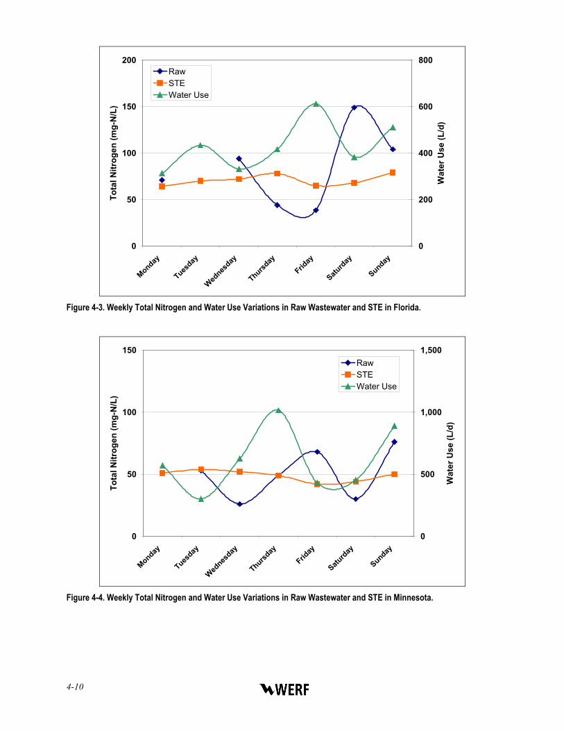
4-10
0
50
100
150
200
Monday
Tuesday
Wednes
day
Thursday
Friday
Saturd
ay
Sunday
Tota
l Nitr
ogen
(mg-
N/L
)
0
200
400
600
800
Wat
er U
se (L
/d)
RawSTEWater Use
Figure 4-3. Weekly Total Nitrogen and Water Use Variations in Raw Wastewater and STE in Florida.
0
50
100
150
Monday
Tuesday
Wednes
day
Thursday
Friday
Saturd
ay
Sunday
Tota
l Nitr
ogen
(mg-
N/L
)
0
500
1,000
1,500
Wat
er U
se (L
/d)
RawSTEWater Use
Figure 4-4. Weekly Total Nitrogen and Water Use Variations in Raw Wastewater and STE in Minnesota.
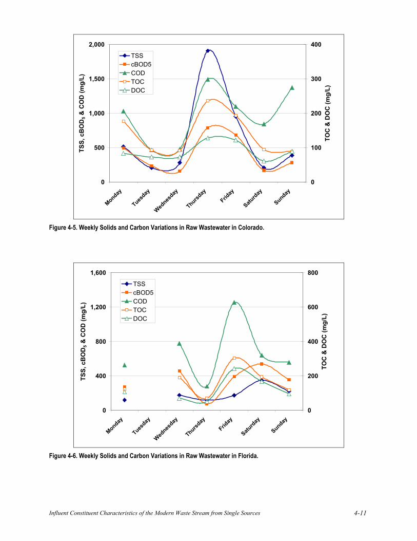
Influent Constituent Characteristics of the Modern Waste Stream from Single Sources 4-11
0
500
1,000
1,500
2,000
Monday
Tuesday
Wednes
day
Thursday
Friday
Saturd
ay
Sunday
TSS,
cB
OD
5 & C
OD
(mg/
L)
0
100
200
300
400
TOC
& D
OC
(mg/
L)
TSScBOD5CODTOCDOC
Figure 4-5. Weekly Solids and Carbon Variations in Raw Wastewater in Colorado.
0
400
800
1,200
1,600
Monday
Tuesday
Wednes
day
Thursday
Friday
Saturd
ay
Sunday
TSS,
cB
OD
5 & C
OD
(mg/
L)
0
200
400
600
800
TOC
& D
OC
(mg/
L)
TSScBOD5CODTOCDOC
Figure 4-6. Weekly Solids and Carbon Variations in Raw Wastewater in Florida.

4-12
0
300
600
900
1,200
1,500
1,800
Monday
Tuesday
Wednes
day
Thursday
Friday
Saturd
ay
Sunday
TSS,
cB
OD
5 & C
OD
(mg/
L)
0
100
200
300
400
500
600
TOC
& D
OC
(mg/
L)
TSScBOD5CODTOCDOC
Figure 4-7. Weekly Solids and Carbon Variations in Raw Wastewater in Minnesota.
1.E+03
1.E+04
1.E+05
1.E+06
1.E+07
1.E+08
1.E+09
Monday
Tuesday
Wednes
day
Thursday
Friday
Saturd
ay
Sunday
Monday
Tuesday
MPN
/100
mL
CO-Raw FL-Raw MN-Raw
Figure 4-8. Weekly Fecal Coliform Bacteria Variations in Raw Wastewater.
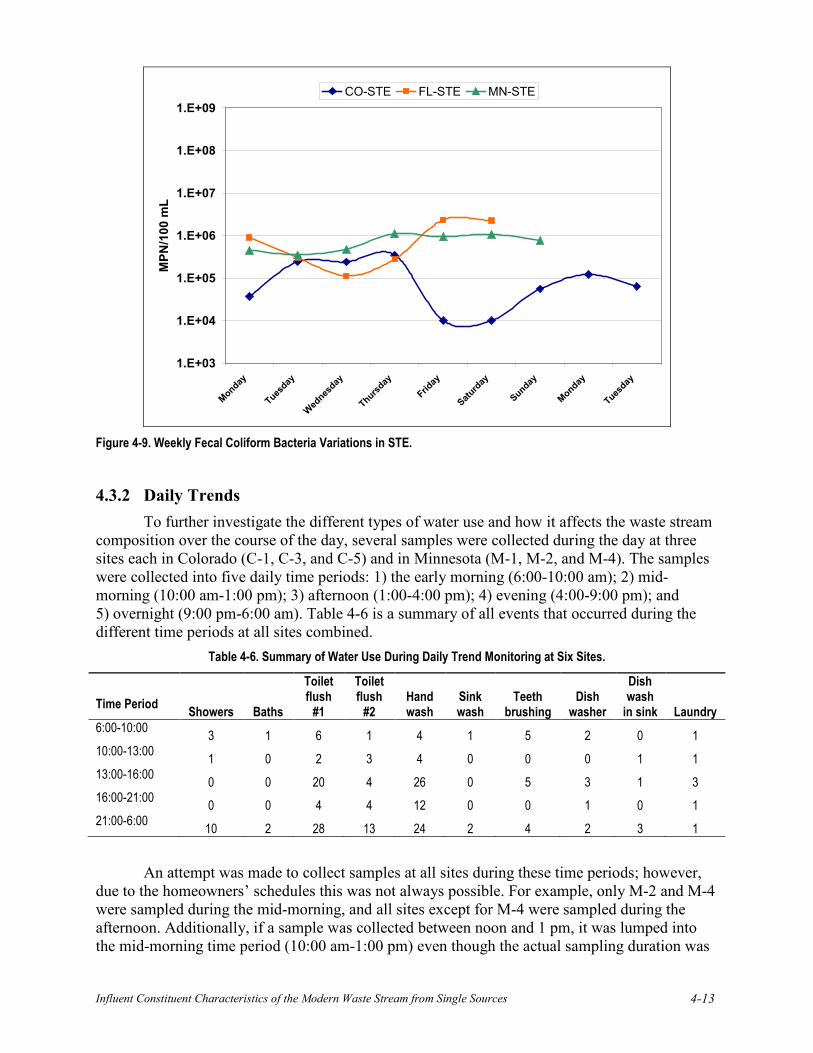
Influent Constituent Characteristics of the Modern Waste Stream from Single Sources 4-13
1.E+03
1.E+04
1.E+05
1.E+06
1.E+07
1.E+08
1.E+09
Monday
Tuesday
Wednes
day
Thursday
Friday
Saturd
ay
Sunday
Monday
Tuesday
MPN
/100
mL
CO-STE FL-STE MN-STE
Figure 4-9. Weekly Fecal Coliform Bacteria Variations in STE.
4.3.2 Daily Trends To further investigate the different types of water use and how it affects the waste stream
composition over the course of the day, several samples were collected during the day at three sites each in Colorado (C-1, C-3, and C-5) and in Minnesota (M-1, M-2, and M-4). The samples were collected into five daily time periods: 1) the early morning (6:00-10:00 am); 2) mid-morning (10:00 am-1:00 pm); 3) afternoon (1:00-4:00 pm); 4) evening (4:00-9:00 pm); and 5) overnight (9:00 pm-6:00 am). Table 4-6 is a summary of all events that occurred during the different time periods at all sites combined.
Table 4-6. Summary of Water Use During Daily Trend Monitoring at Six Sites.
Time Period Showers Baths
Toilet flush
#1
Toilet flush
#2 Hand wash
Sink wash
Teeth brushing
Dish washer
Dish wash
in sink Laundry 6:00-10:00 3 1 6 1 4 1 5 2 0 1 10:00-13:00 1 0 2 3 4 0 0 0 1 1 13:00-16:00 0 0 20 4 26 0 5 3 1 3 16:00-21:00 0 0 4 4 12 0 0 1 0 1 21:00-6:00 10 2 28 13 24 2 4 2 3 1
An attempt was made to collect samples at all sites during these time periods; however, due to the homeowners’ schedules this was not always possible. For example, only M-2 and M-4 were sampled during the mid-morning, and all sites except for M-4 were sampled during the afternoon. Additionally, if a sample was collected between noon and 1 pm, it was lumped into the mid-morning time period (10:00 am-1:00 pm) even though the actual sampling duration was
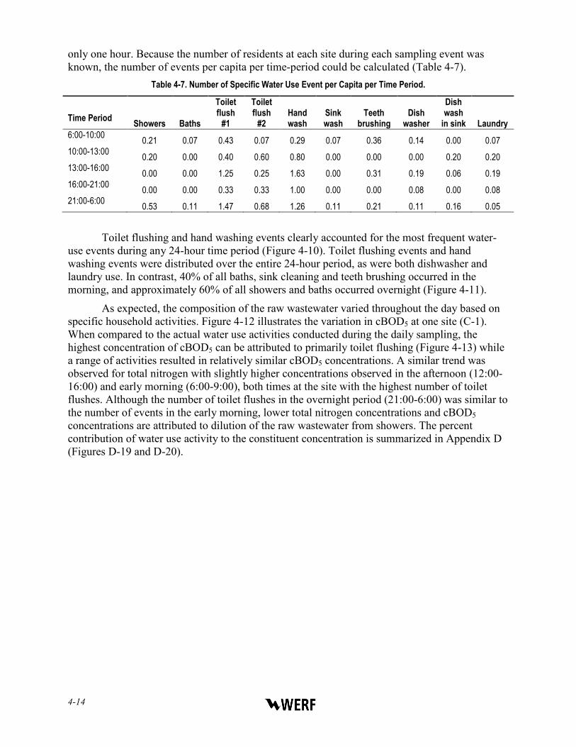
4-14
only one hour. Because the number of residents at each site during each sampling event was known, the number of events per capita per time-period could be calculated (Table 4-7).
Table 4-7. Number of Specific Water Use Event per Capita per Time Period.
Time Period Showers Baths
Toilet flush
#1
Toilet flush
#2 Hand wash
Sink wash
Teeth brushing
Dish washer
Dish wash
in sink Laundry 6:00-10:00 0.21 0.07 0.43 0.07 0.29 0.07 0.36 0.14 0.00 0.07 10:00-13:00 0.20 0.00 0.40 0.60 0.80 0.00 0.00 0.00 0.20 0.20 13:00-16:00 0.00 0.00 1.25 0.25 1.63 0.00 0.31 0.19 0.06 0.19 16:00-21:00 0.00 0.00 0.33 0.33 1.00 0.00 0.00 0.08 0.00 0.08 21:00-6:00 0.53 0.11 1.47 0.68 1.26 0.11 0.21 0.11 0.16 0.05
Toilet flushing and hand washing events clearly accounted for the most frequent water-use events during any 24-hour time period (Figure 4-10). Toilet flushing events and hand washing events were distributed over the entire 24-hour period, as were both dishwasher and laundry use. In contrast, 40% of all baths, sink cleaning and teeth brushing occurred in the morning, and approximately 60% of all showers and baths occurred overnight (Figure 4-11).
As expected, the composition of the raw wastewater varied throughout the day based on specific household activities. Figure 4-12 illustrates the variation in cBOD5 at one site (C-1). When compared to the actual water use activities conducted during the daily sampling, the highest concentration of cBOD5 can be attributed to primarily toilet flushing (Figure 4-13) while a range of activities resulted in relatively similar cBOD5 concentrations. A similar trend was observed for total nitrogen with slightly higher concentrations observed in the afternoon (12:00-16:00) and early morning (6:00-9:00), both times at the site with the highest number of toilet flushes. Although the number of toilet flushes in the overnight period (21:00-6:00) was similar to the number of events in the early morning, lower total nitrogen concentrations and cBOD5 concentrations are attributed to dilution of the raw wastewater from showers. The percent contribution of water use activity to the constituent concentration is summarized in Appendix D (Figures D-19 and D-20).
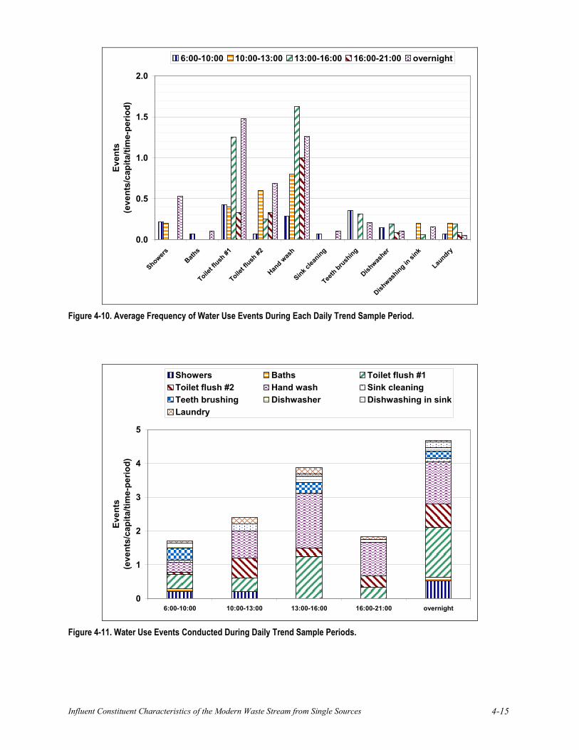
Influent Constituent Characteristics of the Modern Waste Stream from Single Sources 4-15
0.0
0.5
1.0
1.5
2.0
ShowersBath
s
Toilet fl
ush #1
Toilet fl
ush #2
Hand w
ash
Sink clea
ning
Teeth bru
shing
Dishwas
her
Dishwas
hing in si
nk
Laundry
Even
ts
(eve
nts/
capi
ta/ti
me-
perio
d)
6:00-10:00 10:00-13:00 13:00-16:00 16:00-21:00 overnight
Figure 4-10. Average Frequency of Water Use Events During Each Daily Trend Sample Period.
0
1
2
3
4
5
6:00-10:00 10:00-13:00 13:00-16:00 16:00-21:00 overnight
Even
ts
(eve
nts/
capi
ta/ti
me-
perio
d)
Showers Baths Toilet flush #1Toilet flush #2 Hand wash Sink cleaningTeeth brushing Dishwasher Dishwashing in sinkLaundry
Figure 4-11. Water Use Events Conducted During Daily Trend Sample Periods.
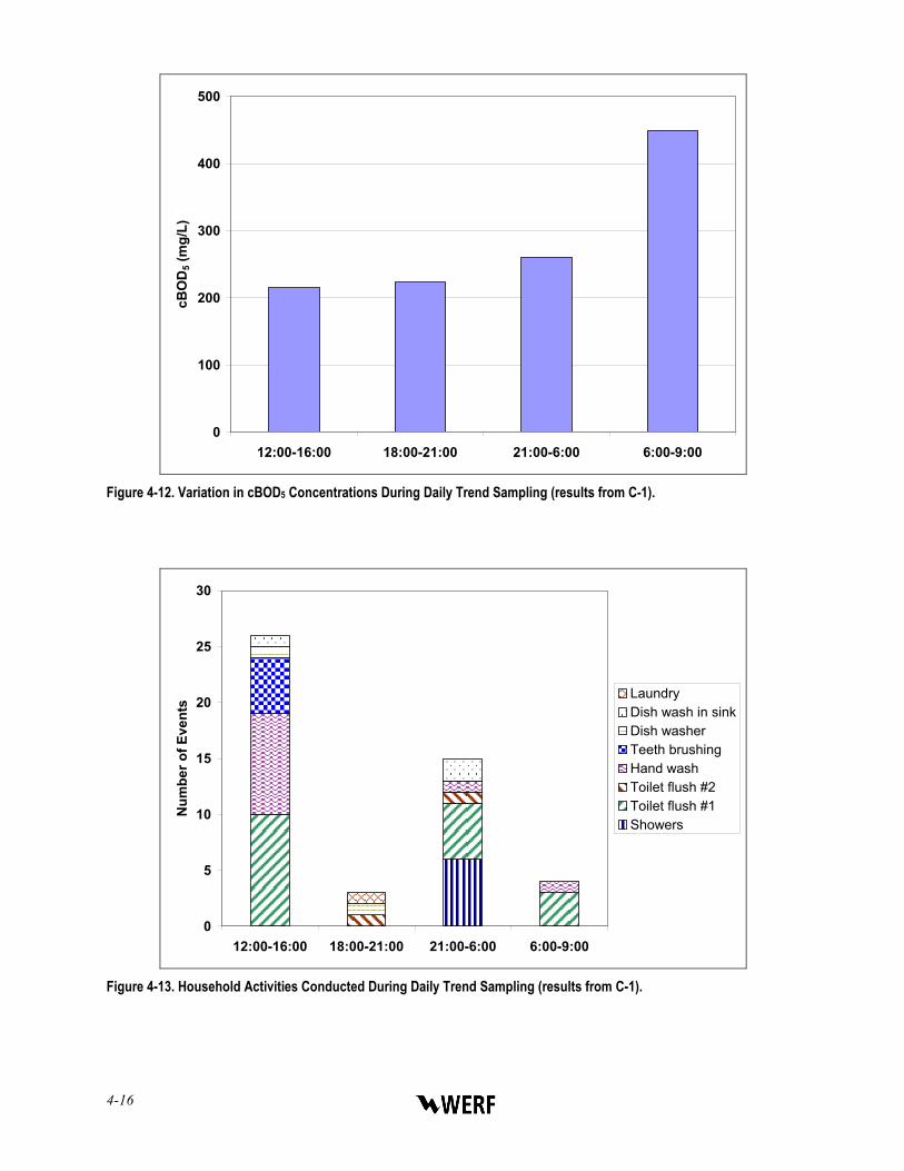
4-16
0
100
200
300
400
500
12:00-16:00 18:00-21:00 21:00-6:00 6:00-9:00
cBO
D5 (
mg/
L)
Figure 4-12. Variation in cBOD5 Concentrations During Daily Trend Sampling (results from C-1).
0
5
10
15
20
25
30
12:00-16:00 18:00-21:00 21:00-6:00 6:00-9:00
Num
ber o
f Eve
nts
LaundryDish wash in sinkDish washerTeeth brushingHand washToilet flush #2Toilet flush #1Showers
Figure 4-13. Household Activities Conducted During Daily Trend Sampling (results from C-1).

Influent Constituent Characteristics of the Modern Waste Stream from Single Sources 4-17
4.3.3 Source Activities and Tier 3 Composition Homeowners voluntarily provided information about the types and brand names of
consumer product chemicals used in their homes, such as shampoo, bar soap, hand soap, toothpaste, dishwashing detergent, laundry detergent, lotion, and cleaning supplies. In addition, during each 24-hour raw wastewater sample collection event, the homeowners recorded the type and number of water- and chemical-consuming activities that contributed to the wastewater flow, such as the number of hand washes, toilet flushes, tooth brushing events, showers, baths, dish washer loads, clothes washer loads, cleaning events, and any other wastewater-producing activities.
All dish and laundry detergents used in the homes contained unspecified “surfactants”, which likely include nonylphenolethoxylate surfactants that can contain or degrade to 4-nonylphenol and NP1EO. All households used products listing as an ingredient the metal-chelating agent EDTA (found in shampoo, bar soap, hand soap, detergent, and lotion) and the antimicrobial triclosan (found in bar soap, hand soap, and toothpaste).
During the fall sampling, the concentration of triclosan was 225 μg/L in the raw wastewater at site C-1. During this 24-sampling event, the homeowners reported 38 triclosan-consuming events, including showers using bar soap, hand washes using hand soap, and teeth brushing using toothpaste. In contrast, concentrations of triclosan in raw wastewater from sites C-3, F-4, and F-2 were at least 10 times lower than C-1 levels and three or fewer triclosan-using events were reported at each of these sites during the same time period (Figure 4-14).
0
10
20
30
40
C-1 C-3 F-2 F-4
Site ID
Num
ber o
f Eve
nts
Hand soap
Body soap
Toothpaste
225
200.6 3.7
0
50
100
150
200
250
C-1 C-3 F-2 F-4
Site ID
Con
cent
ratio
n (u
g/L)
Triclosan
Figure 4-14. Comparison of Triclosan-consuming Events and Raw Wastewater Concentrations during the 24-hour Fall Sampling Event.

4-18
Site F-2 had measurable levels of triclosan in the raw wastewater (0.55 μg/L) though there were no reported triclosan-consuming events. This suggests that there may have been one or more unreported triclosan-consuming events or unreported consumer product chemicals containing triclosan in use at the home. The homeowners at site F-4 reported no use of antibacterial agents in the house in the written survey; however, the reported brand of toothpaste contained triclosan and the compound was measured in the raw wastewater (3.7 μg/L).
The occurrence and levels of EDTA also illustrated the impacts on the raw wastewater composition of water- and chemical-consuming events in the home (Figure 4-15). Site C-1 reported 33 EDTA-consuming events (e.g., laundry loads, hand washes, and showers using soap and shampoo) as compared to four and six reported events at sites C-3 and F-4, respectively. The EDTA raw wastewater concentration was approximately 10 times higher at C-1 than C-3 and F-4. The EDTA raw wastewater concentration was very high at site F-2 (~10 to 100x higher than the other sites). Though the number of reported EDTA-using events of seven was relatively low, one of the events was a clothes washing laundry load, which likely contributed much more mass of chemical to the onsite system than, for example, a single hand-washing event.
0
10
20
30
40
C-1 C-3 F-2 F-4
Site ID
Num
ber o
f Eve
nts
Body SoapShampooLotionLaundryHand soap
0
20
40
60
80
100
C-1 C-3 F-2 F-4
Site ID
Con
cent
ratio
n (u
g/L)
EDTA
E 720
59
6.4 6.8
Figure 4-15. Comparison of EDTA-Consuming Events and Raw Wastewater Concentrations during the 24-hour Fall Sampling Event.
The concentration of 4-nonylphenol in raw wastewater was relatively similar (between 20 and 70 μg/L) in sites C-1, C-3, and F-2, which each reported between two and four “surfactant”-consuming events including at least one clothes washing laundry load (Figure 4-15). The 4-nonylphenol concentration in the raw wastewater from site F-4 was between four and ten times lower than the other sites, which is hypothesized to be due to one or a combination of the following factors: 1) fewer “surfactant”-consuming events (1 vs. 2 to 4), 2) no laundry contribution, which may be the largest contributor of 4-nonylphenol, or 3) a dilution effect from

Influent Constituent Characteristics of the Modern Waste Stream from Single Sources 4-19
high toilet flushing (Figure 4-16, 44 reported toilet flushes vs. <20 at the other sites). These results suggest that knowledge of the water- and chemical-consuming events at the site may provide some information regarding the occurrence and concentration levels of consumer product chemicals in single-source raw wastewater.
0
1
2
3
4
5
C-1 C-3 F-2 F-4
Site ID
Num
ber o
f Eve
nts
Laundry
Dishwasher
23
37
66
6.3
0
20
40
60
80
C-1 C-3 F-2 F-4
Site ID
Con
cent
ratio
n (u
g/L)
Nonylphenol
0
10
20
30
40
50
C-1 C-3 F-2 F-4
Site ID
Num
ber o
f Eve
nts
Toiletflush
Figure 4-16. Comparison of Nonylphenol-consuming Events and Raw Wastewater Concentrations during the 24-hour Fall Sampling Event.
According to the questionnaires filled out by the residents of the studied sites, a list of potential pharmaceutical residues that might be detected in the raw wastewater as well as the STE samples was assembled (Table 4-8). Overlap between the employed method and the active ingredients is indicated by a check mark in Table 4-8. Check marks in parentheses indicate derivates of salicylic acid that may be potentially transformed to salicylic acid before excretion or during onsite treatment.

4-20
Table 4-8. Reported Pharmaceutical Use at the Field Sites.
Site Brand or Generic Name Active Ingredients Use Detectable
w/method
C-1
Prescription Lipitor® Atorvastatin calcium Blood lipid regulator Tricor® Fenofibrate Blood lipid regulator √
Non-prescription
Aspirin Acetyl salicylic acid Pain reliever (√) Ibuprofen Ibuprofen Anti-inflammatory drug √
Acetaminophen Acetaminophen Pain reliever
C-3 Prescription
Diltiazem Diltiazem hydrochloride Hypertension drug Enalapril Enalapril maleate Hypertension drug Norvasc® Amlodipine besylate Hypertension drug Crestor® Rosuvastatin calcium Blood lipid regulator
Metolazone Metolazone Diuretic/Hypertension drug Metformin Metformin hydrochloride Anti-diabetic drug
Non-prescription Prilosec® Omeprazole Antacid
F-2 Non-prescription
Tums® Calcium carbonate Antacid Tylenol® Acetaminophen Pain reliever Aleve® Naproxen Anti-inflammatory drug √
Zantac® Ranitidine hydrochloride Antacid
Motrin® Ibuprofen Pseudoephedrine hydrochloride
Anti-inflammatory drug Decongestant
√
Sudafed® Pseudoephedrine hydrochloride Decongestant
F-4 Prescription
GLY/METFRM unknown unknown Actos® Pioglitazone hydrochloride Antidiabetic
Norvasc® Amlodipine besylate Hypertension drug Spironolactone Spironolactone Diuretic drug
Avalide® Irbesartan Hydrochlorothiazide
Hypertension drug Diuretic drug
Lisinopril Lisinopril Hypertension drug Clonidine Clonidine Hypertension drug
Spiriva® Tiotropium bromide Chronic obstructive pulmonary disease treatment
Advair® Fluticasone propionate Salmeterol xinafoate
Corticosteroid Bronchodilator aerosol
Albuterol Albuterol Bronchodilator aerosol Guaifenesin Guaifenesin Expectorant
Non-prescription Aspirin Acetyl salicylic acid Pain reliever (√)
M-1
Prescription Asacol® Mesalamine Anti-inflammatory drug (√)
Non-prescription
Excedrin® Acetaminophin
Acetyl salicylic acid Caffeine
Pain reliever Pain reliever
Stimulant
(√)
Aspirin Acetyl salicylic acid Pain reliever (√)
M-3 Non-prescription
Tylenol® Acetaminophen Pain reliever Imodium® Loperamide hydrochloride Diarrhea treatment
(√) indicates salicylic acid derivates; might account for some of the salicylic acid concentration in the samples
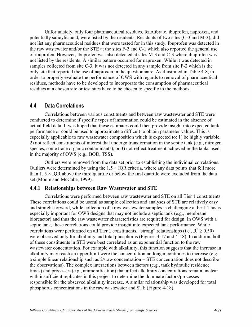
Influent Constituent Characteristics of the Modern Waste Stream from Single Sources 4-21
Unfortunately, only four pharmaceutical residues, fenofibrate, ibuprofen, naproxen, and potentially salicylic acid, were listed by the residents. Residents of two sites (C-3 and M-3), did not list any pharmaceutical residues that were tested for in this study. Ibuprofen was detected in the raw wastewater and/or the STE at the sites F-2 and C-1 which also reported the general use of ibuprofen. However, ibuprofen was also detected at sites M-3 and C-3 where ibuprofen was not listed by the residents. A similar pattern occurred for naproxen. While it was detected in samples collected from site C-3, it was not detected in any sample from site F-2 which is the only site that reported the use of naproxen in the questionnaire. As illustrated in Table 4-8, in order to properly evaluate the performance of OWS with regards to removal of pharmaceutical residues, methods have to be developed to incorporate the consumption of pharmaceutical residues at a chosen site or test sites have to be chosen to specific to the methods.
4.4 Data Correlations Correlations between various constituents and between raw wastewater and STE were
conducted to determine if specific types of information could be estimated in the absence of actual field data. It was hoped that these estimates could then provide insight into expected tank performance or could be used to approximate a difficult to obtain parameter values. This is especially applicable to raw wastewater composition which is expected to: 1) be highly variable, 2) not reflect constituents of interest that undergo transformation in the septic tank (e.g., nitrogen species, some trace organic contaminants), or 3) not reflect treatment achieved in the tanks used in the majority of OWS (e.g., BOD, TSS).
Outliers were removed from the data set prior to establishing the individual correlations. Outliers were determined by using the 1.5 × IQR criteria, where any data points that fell more than 1. 5 × IQR above the third quartile or below the first quartile were excluded from the data set (Moore and McCabe, 1999).
4.4.1 Relationships between Raw Wastewater and STE Correlations were performed between raw wastewater and STE on all Tier 1 constituents.
These correlations could be useful as sample collection and analyses of STE are relatively easy and straight forward, while collection of a raw wastewater samples is challenging at best. This is especially important for OWS designs that may not include a septic tank (e.g., membrane bioreactor) and thus the raw wastewater characteristics are required for design. In OWS with a septic tank, these correlations could provide insight into expected tank performance. While correlations were performed on all Tier 1 constituents, “strong” relationships (i.e., R2 ≥ 0.50) were observed only for alkalinity and total phosphorus (Figures 4-17 and 4-18). In addition, both of these constituents in STE were best correlated as an exponential function to the raw wastewater concentration. For example with alkalinity, this function suggests that the increase in alkalinity may reach an upper limit were the concentration no longer continues to increase (e.g., a simple linear relationship such as 2×raw concentration = STE concentration does not describe the observations). The complex interactions between factors (e.g., tank hydraulic residence times) and processes (e.g., ammonification) that affect alkalinity concentrations remain unclear with insufficient replicates in this project to determine the dominate factors/processes responsible for the observed alkalinity increase. A similar relationship was developed for total phosphorus concentrations in the raw wastewater and STE (Figure 4-18).

4-22
Alkalinity in STE = 40(Alkalinity in Raw Wastewater)0.42
R2 = 0.51n = 63
0
200
400
600
800
1,000
0 100 200 300 400 500 600 700Alkalinity in Raw Wastewater (mg-CaCO3/L)
Alk
alin
ity in
STE
(mg-
CaC
O3/L
)
Figure 4-17. Correlation between Alkalinity in Raw Wastewater and STE (data from all sites).
TP in STE = 2.5 (TP in Raw Wastewater)0.55
R2 = 0.51n = 57
(outliers excluded)
0
5
10
15
20
25
30
0 5 10 15 20 25 30Total Phosphorus in Raw Wastewater (mg-P/L)
Tota
l Pho
spho
rus
in S
TE (m
g-P/
L)
Figure 4-18. Correlation between Total Phosphorus in Raw Wastewater and STE (data from all sites, excluding outliers).
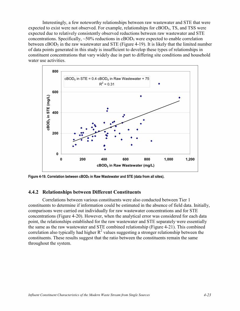
Influent Constituent Characteristics of the Modern Waste Stream from Single Sources 4-23
Interestingly, a few noteworthy relationships between raw wastewater and STE that were expected to exist were not observed. For example, relationships for cBOD5, TS, and TSS were expected due to relatively consistently observed reductions between raw wastewater and STE concentrations. Specifically, ~50% reductions in cBOD5 were expected to enable correlation between cBOD5 in the raw wastewater and STE (Figure 4-19). It is likely that the limited number of data points generated in this study is insufficient to develop these types of relationships in constituent concentrations that vary widely due in part to differing site conditions and household water use activities.
cBOD5 in STE = 0.4 cBOD5 in Raw Wastewater + 75R2 = 0.31
0
200
400
600
800
0 200 400 600 800 1,000 1,200cBOD5 in Raw Wastewater (mg/L)
cBO
D5 i
n ST
E (m
g/L)
Figure 4-19. Correlation between cBOD5 in Raw Wastewater and STE (data from all sites).
4.4.2 Relationships between Different Constituents Correlations between various constituents were also conducted between Tier 1
constituents to determine if information could be estimated in the absence of field data. Initially, comparisons were carried out individually for raw wastewater concentrations and for STE concentrations (Figure 4-20). However, when the analytical error was considered for each data point, the relationships established for the raw wastewater and STE separately were essentially the same as the raw wastewater and STE combined relationship (Figure 4-21). This combined correlation also typically had higher R2 values suggesting a stronger relationship between the constituents. These results suggest that the ratio between the constituents remain the same throughout the system.
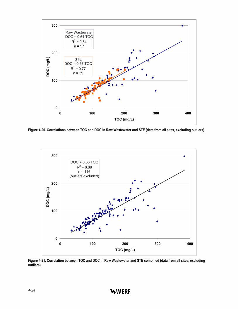
4-24
Raw WastewaterDOC = 0.64 TOC
R2 = 0.54n = 57
STEDOC = 0.67 TOC
R2 = 0.77n = 59
0
100
200
300
0 100 200 300 400TOC (mg/L)
DO
C (m
g/L)
Figure 4-20. Correlations between TOC and DOC in Raw Wastewater and STE (data from all sites, excluding outliers).
DOC = 0.65 TOCR2 = 0.68n = 116
(outliers excluded)
0
100
200
300
0 100 200 300 400TOC (mg/L)
DO
C (m
g/L)
Figure 4-21. Correlation between TOC and DOC in Raw Wastewater and STE combined (data from all sites, excluding outliers).

Influent Constituent Characteristics of the Modern Waste Stream from Single Sources 4-25
Typically the BOD5 test is the most used analytical method to assess wastewater by measuring the biodegradable portion of organic material in the wastewater. However, there are several limitations to the test such as the test is time consuming, the five-day value is a function of the test methods and not the true total oxygen demand, and particles in the wastewater may have an impact on the test. Alternatively, the COD test consists of oxidizing the sample and then measuring the oxygen required for the chemical oxidation. While, the COD test measures the oxygen equivalent of the organic material present in the wastewater, it cannot differentiate between nondegradable and biodegradable organic materials. However, the COD test takes about four hours and requires minimal laboratory experience and equipment. The correlation between COD and cBOD5 (Figure 4-22) can be useful for approximating cBOD5 concentrations in either raw wastewater or STE. For example, if the COD in a waste is 1,000 mg/L, then the cBOD5 concentration can be estimated based on the correlation equation in Figure 4-22. In this case, cBOD5 would be ~592 mg/L (e.g., cBOD5 = (COD – 206)/1.34).
COD = 1.34 cBOD5 + 206R2 = 0.55n = 110
(outliers excluded)
0
500
1,000
1,500
2,000
0 200 400 600 800 1,000cBOD5 (mg/L)
CO
D (m
g/L)
Figure 4-22. Correlation between cBOD5 and COD in Raw Wastewater and STE combined (data from all sites, excluding outliers).
TOC is a convenient measurement of the total organic content, but it does not measure organically bound elements such as nitrogen, hydrogen or other inorganic compounds that may contribute to the oxygen demand. However, similar correlations may be used to estimate accompanying wastewater COD or BOD (for raw wastewater and STE). The correlation made between TOC and COD was TOC = 0.22×COD (R2=0.67) and for TOC and cBOD5 was TOC = 0.24×cBOD5 (R2=0.43).
Similar to relationships between raw wastewater and STE, a few noteworthy relationships that were expected to exist were not observed. For example, a relationship between pH and alkalinity could not be established due to the low variability in pH range (e.g., the relationship resulted in either a vertical or horizontal line which suggested all ranges of alkalinity in the tank would predict the same pH value). Another expected relationship between alkalinity and
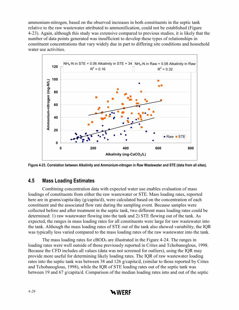
4-26
ammonium-nitrogen, based on the observed increases in both constituents in the septic tank relative to the raw wastewater attributed to ammonification, could not be established (Figure 4-23). Again, although this study was extensive compared to previous studies, it is likely that the number of data points generated was insufficient to develop these types of relationships in constituent concentrations that vary widely due in part to differing site conditions and household water use activities.
NH4-N in Raw = 0.08 Alkalinity in RawR2 = 0.32
NH4-N in STE = 0.06 Alkalinity in STE + 34R2 = 0.16
0
20
40
60
80
100
120
0 200 400 600 800Alkalinity (mg-CaCO3/L)
Am
mon
ium
-nitr
ogen
(mg-
N/L
)
Raw STE
Figure 4-23. Correlation between Alkalinity and Ammonium-nitrogen in Raw Wastewater and STE (data from all sites).
4.5 Mass Loading Estimates Combining concentration data with expected water use enables evaluation of mass
loadings of constituents from either the raw wastewater or STE. Mass loading rates, reported here are in grams/capita/day (g/capita/d), were calculated based on the concentration of each constituent and the associated flow rate during the sampling event. Because samples were collected before and after treatment in the septic tank, two different mass loading rates could be determined: 1) raw wastewater flowing into the tank and 2) STE flowing out of the tank. As expected, the ranges in mass loading rates for all constituents were large for raw wastewater into the tank. Although the mass loading rates of STE out of the tank also showed variability, the IQR was typically less varied compared to the mass loading rates of the raw wastewater into the tank.
The mass loading rates for cBOD5 are illustrated in the Figure 4-24. The ranges in loading rates were well outside of those previously reported in Crites and Tchobanoglous, 1998. Because the CFD includes all values (data was not screened for outliers), using the IQR may provide more useful for determining likely loading rates. The IQR of raw wastewater loading rates into the septic tank was between 38 and 126 g/capita/d, (similar to those reported by Crites and Tchobanoglous, 1998), while the IQR of STE loading rates out of the septic tank was between 19 and 67 g/capita/d. Comparison of the median loading rates into and out of the septic

Influent Constituent Characteristics of the Modern Waste Stream from Single Sources 4-27
tank (68 and 32 g/capita/d respectively) suggested cBOD5 mass removal of approximately 50% in the septic tank. Similar mass loading rate trends were found for COD (Figure 4-25).
0
20
40
60
80
100
0 100 200 300 400cBOD5 Loading Rates (g/capita/d)
Cum
ulat
ive
Freq
uenc
y (%
)
Loading Rates of Raw Wastewater into Septic Tank (n=62)
Loading Rates of STE out of Septic Tank (n=59)
Figure 4-24. Mass Loading Rates for cBOD5.
0
20
40
60
80
100
0 200 400 600 800 1,000 1,200COD Loading Rates (g/capita/d)
Cum
ulat
ive
Freq
uenc
y (%
)
Loading Rates of Raw Wastewater into Septic Tank (n=63)
Loading Rates of STE out of Septic Tank (n=60)
Figure 4-25. Mass Loading Rates for COD.
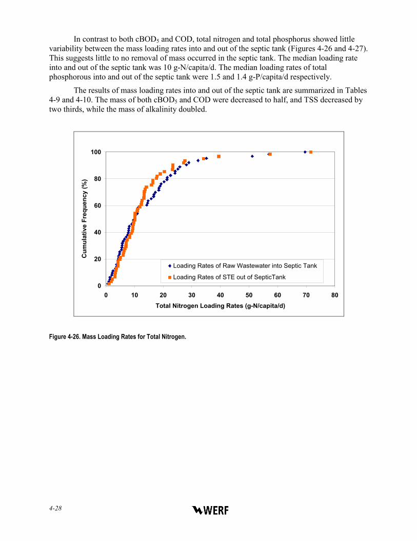
4-28
In contrast to both cBOD5 and COD, total nitrogen and total phosphorus showed little variability between the mass loading rates into and out of the septic tank (Figures 4-26 and 4-27). This suggests little to no removal of mass occurred in the septic tank. The median loading rate into and out of the septic tank was 10 g-N/capita/d. The median loading rates of total phosphorous into and out of the septic tank were 1.5 and 1.4 g-P/capita/d respectively.
The results of mass loading rates into and out of the septic tank are summarized in Tables 4-9 and 4-10. The mass of both cBOD5 and COD were decreased to half, and TSS decreased by two thirds, while the mass of alkalinity doubled.
0
20
40
60
80
100
0 10 20 30 40 50 60 70 80Total Nitrogen Loading Rates (g-N/capita/d)
Cum
ulat
ive
Freq
uenc
y (%
)
Loading Rates of Raw Wastewater into Septic Tank
Loading Rates of STE out of SepticTank
Figure 4-26. Mass Loading Rates for Total Nitrogen.

Influent Constituent Characteristics of the Modern Waste Stream from Single Sources 4-29
0
20
40
60
80
100
0 5 10 15 20Total Phosphorus Loading Rates (g-P/capita/d)
Cum
ulat
ive
Freq
uenc
y(%
)
Loading Rates of Raw Wastewater into Septic Tank
Loading Rates of STE out of Septic Tank
Figure 4-27. Mass Loading Rates for Total Phosphorus.
Table 4-9. Summary of Mass Loading Rates of Raw Wastewater into the Septic Tank (g/capita/d).
Constituent Mean Std. Dev. Min Max Median Alkalinity (as CaCO3) 41 39 4 176 30 TSS 80 93 2 401 42 cBOD5 90 77 8 378 68 COD 189 193 14 1088 125 Total Nitrogen 14.2 13.3 0.6 69.6 10.1 Total Phosphorus 3.6 4.9 0 31.7 1.9
Table 4-10. Summary of Mass Loading Rates of STE out of the Septic Tank (g/capita/d).
Constituent Mean Std. Dev. Min Max Median Alkalinity (as CaCO3) 95 103 7 474 67 TSS 22 39 1 270 13 cBOD5 52 48 4 239 33 COD 98 91 10 420 57 Total Nitrogen 13.3 12.3 1.1 71.6 10.1 Total Phosphorus 2.5 3.4 0 15.9 1.4
Regional mass loading rate trends were observed for several Tier 1 constituents,
including cBOD5, COD, total nitrogen, ammonium-nitrogen, and total phosphorus. Mass loading rates of both raw wastewater into the tank and STE out of the tank were found to be much higher in Colorado compared to in both Florida and Minnesota. For example, the STE mass loading rates for cBOD5 in Colorado were 140% greater than in Florida, and 75% greater than in Minnesota, while the STE mass loading rates for COD were 92% greater than in Florida, and

4-30
62% greater than in Minnesota (Figure 4-28). Similar results were found for nutrients, where the STE mass loading rates for total nitrogen were 58% greater than in Florida, and 46% greater than in Minnesota, 70% and 73% greater respectively for NH3, and for total phosphorous, the rates were 93% greater than in Florida and over 142% greater than those in Minnesota (Figure 4-29).
0
50
100
150
200
250
Into Tank Out of Tank Into Tank Out of Tank
cBOD5 COD
Mas
s Lo
adin
g R
ates
(g/c
apita
/d)
Colorado Florida Minnesota
Figure 4-28. Average Mass Loading Rates for cBOD5 and COD by Region.
0
5
10
15
20
Into Tank Out of Tank Into Tank Out of Tank Into Tank Out of Tank
Total Nitrogen Ammonium Total Phosphorus
Mas
s Lo
adin
g R
ates
(g/c
apita
/d)
Colorado Florida Minnesota
Figure 4-29. Average Mass Loading Rates for Nutrients by Region.

Influent Constituent Characteristics of the Modern Waste Stream from Single Sources 4-31
It is interesting to note that all sites in Colorado use an in-sink garbage grinder, compared to only one site in Florida and one in Minnesota. However, it is unlikely that the disposals account for all of the high mass loading rates in Colorado. Crites and Tchobanoglous (1998) report 10-25% higher mass loading rates of raw wastewater into the septic tank from a household with a garbage grinder compared to households without a grinder.
Mass loading rate trends were also observed for occupant age for several Tier 1 constituents, including cBOD5, COD, total nitrogen, ammonium-nitrogen, and total phosphorus. Mass loading rates of both raw wastewater into the septic tank and STE out of the tank were found to be much higher in households where the occupants were older than 65. For example, the mean raw wastewater mass loading rate into the septic tank for cBOD5 was 59 g/capita/d in households where occupants were younger than 65 and 144 g/capita/d in households where occupants were older than 65 (Figure 4-30). Similar results were observed for STE mass loading out of the septic tank (mean mass loading rates of 34 g/capita/d vs. 90 g/capita/d for occupants younger and older than 65, respectively) (Figure 4-31). Mass loading rates of raw wastewater into the septic tank for all Tier 1 constituents were observed to be 140% to over 300% greater in households with older occupants than in households with younger occupants. The Tier 1 mass loading rates of STE out of the septic tank were 165% to over 300% greater in households with older occupants than in households with younger occupants.
0
100
200
300
400
<65 >65Occupants Age
cBO
D5 L
oadi
ng in
to T
ank
(g/c
apita
/day
) IQR Boxplot
95% CI Mean Diamond
Outliers > 1.5 and < 3 IQR
Figure 4-30. Mass Loading Rates of Raw Wastewater into the Septic Tank for cBOD5 by Age of Occupant.

4-32
0
100
200
300
400
<65 >65Occupants Age
cBO
D5 L
oadi
ng o
ut o
f Tan
k (g
/cap
ita/d
) IQR Boxplot
95% CI Mean Diamond
Outliers > 1.5 and < 3 IQR
Figure 4-31. Mass Loading Rates of STE out of the Septic Tank for cBOD5 by Age of Occupant.
Correlations were also evaluated between the mass loading of the raw wastewater into the tank and of STE out of the tank. It is interesting to note that while correlations could not be established between the raw wastewater and STE concentrations, correlations between mass loading rates had R2 values >0.50. This suggests that the per capita mass loading rates are normalized to the differences between site conditions and are relatively similar and independent of regional location, season, age of the occupant, or number of occupants per household. These correlations also provide insight into expected tank performance which was not captured in the CFDs or correlations of concentrations. For example, a correlation between the mass loading rate of cBOD5 from raw wastewater into the tank and STE out of the tank suggest approximately 50% removal of cBOD5 in the septic tank (Figure 4-32). This finding supports similar estimated removal rates based on average concentration (49%) and average mass loading rate (50%). A similar relationship was observed for COD (Figure 4-33).
However, for total nitrogen and total phosphorus, the correlations between mass loading rates appear to contradict the results as presented on CFDs. In this case, the correlations between the mass loading rate from raw wastewater into the tank and STE out of the tank suggests approximately 20% removal of total nitrogen and ~40% of total phosphorus in the septic tank (Figures 4-34 and 4-35) while the CFDs (see Figures 3-15, 3-19, 4-26, and 4-27) suggest no removal in the tank. The key difference is because the CFD illustrates the relative range of constituent concentrations from an entire data population based on the frequency of the occurrence. Specifically, the 25% value for total nitrogen in raw wastewater may be from one site while the 25% value in STE may be from a different site and/or different sampling event. In both the raw wastewater and STE, the 25% CFD value simply indicates that 25% of the measured values are less than the 25% value. In contrast, the mass loading rate correlations are a paired comparison of the raw wastewater concentration and flow with the STE concentration and flow at a single site during a single sampling event. Thus, the mass loading rate correlation incorporates the actual observed removal of a constituent for all sites and sampling events during the project.
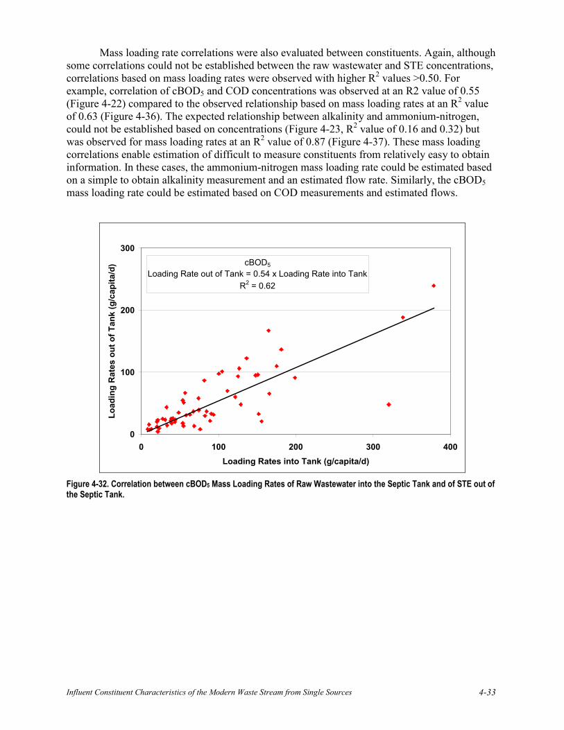
Influent Constituent Characteristics of the Modern Waste Stream from Single Sources 4-33
Mass loading rate correlations were also evaluated between constituents. Again, although some correlations could not be established between the raw wastewater and STE concentrations, correlations based on mass loading rates were observed with higher R2 values >0.50. For example, correlation of cBOD5 and COD concentrations was observed at an R2 value of 0.55 (Figure 4-22) compared to the observed relationship based on mass loading rates at an R2 value of 0.63 (Figure 4-36). The expected relationship between alkalinity and ammonium-nitrogen, could not be established based on concentrations (Figure 4-23, R2 value of 0.16 and 0.32) but was observed for mass loading rates at an R2 value of 0.87 (Figure 4-37). These mass loading correlations enable estimation of difficult to measure constituents from relatively easy to obtain information. In these cases, the ammonium-nitrogen mass loading rate could be estimated based on a simple to obtain alkalinity measurement and an estimated flow rate. Similarly, the cBOD5 mass loading rate could be estimated based on COD measurements and estimated flows.
cBOD5
Loading Rate out of Tank = 0.54 x Loading Rate into TankR2 = 0.62
0
100
200
300
0 100 200 300 400Loading Rates into Tank (g/capita/d)
Load
ing
Rat
es o
ut o
f Tan
k (g
/cap
ita/d
)
Figure 4-32. Correlation between cBOD5 Mass Loading Rates of Raw Wastewater into the Septic Tank and of STE out of the Septic Tank.

4-34
CODLoading Rate out of Tank = 0.53 x Loading Rate into Tank
R2 = 0.63
0
100
200
300
400
500
0 200 400 600 800 1,000Loading Rates into Tank (g/capita/d)
Load
ing
Rat
es o
ut o
f Tan
k (g
/cap
ita/d
)
Figure 4-33. Correlation between COD Mass Loading Rates of Raw Wastewater into the Septic Tank and of STE out of the Septic Tank.
Total NitrogenLoading Rate out of Tank = 0.8 x Loading Rate into Tank
R2 = 0.50
0
20
40
60
0 20 40 60 80Loading Rates into Tank (g/capita/d)
Load
ing
Rat
es o
ut o
f Tan
k (g
/cap
ita/d
)
Figure 4-34. Correlation between Total Nitrogen Mass Loading Rates of Raw Wastewater into the Septic Tank and of STE out of the Septic Tank.
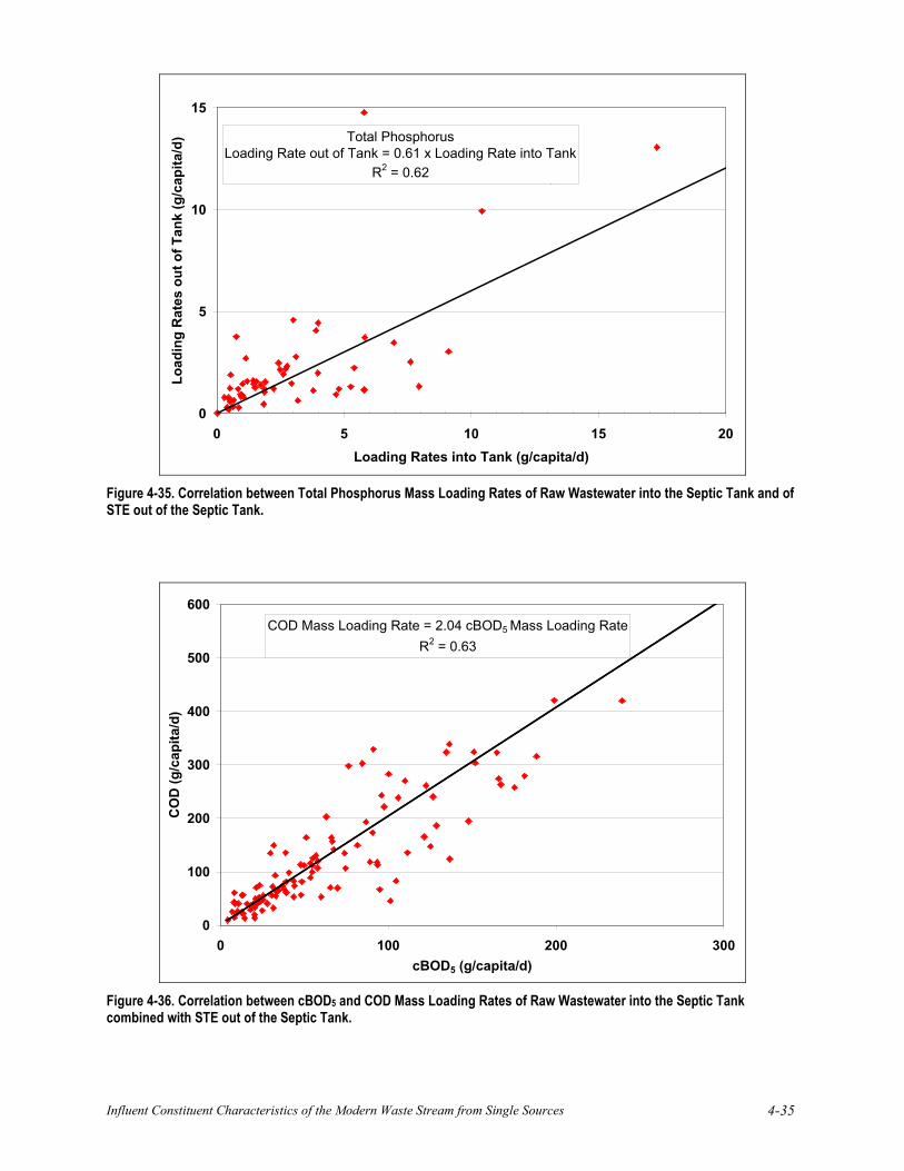
Influent Constituent Characteristics of the Modern Waste Stream from Single Sources 4-35
Total PhosphorusLoading Rate out of Tank = 0.61 x Loading Rate into Tank
R2 = 0.62
0
5
10
15
0 5 10 15 20Loading Rates into Tank (g/capita/d)
Load
ing
Rat
es o
ut o
f Tan
k (g
/cap
ita/d
)
Figure 4-35. Correlation between Total Phosphorus Mass Loading Rates of Raw Wastewater into the Septic Tank and of STE out of the Septic Tank.
COD Mass Loading Rate = 2.04 cBOD5 Mass Loading RateR2 = 0.63
0
100
200
300
400
500
600
0 100 200 300cBOD5 (g/capita/d)
CO
D (g
/cap
ita/d
)
Figure 4-36. Correlation between cBOD5 and COD Mass Loading Rates of Raw Wastewater into the Septic Tank combined with STE out of the Septic Tank.
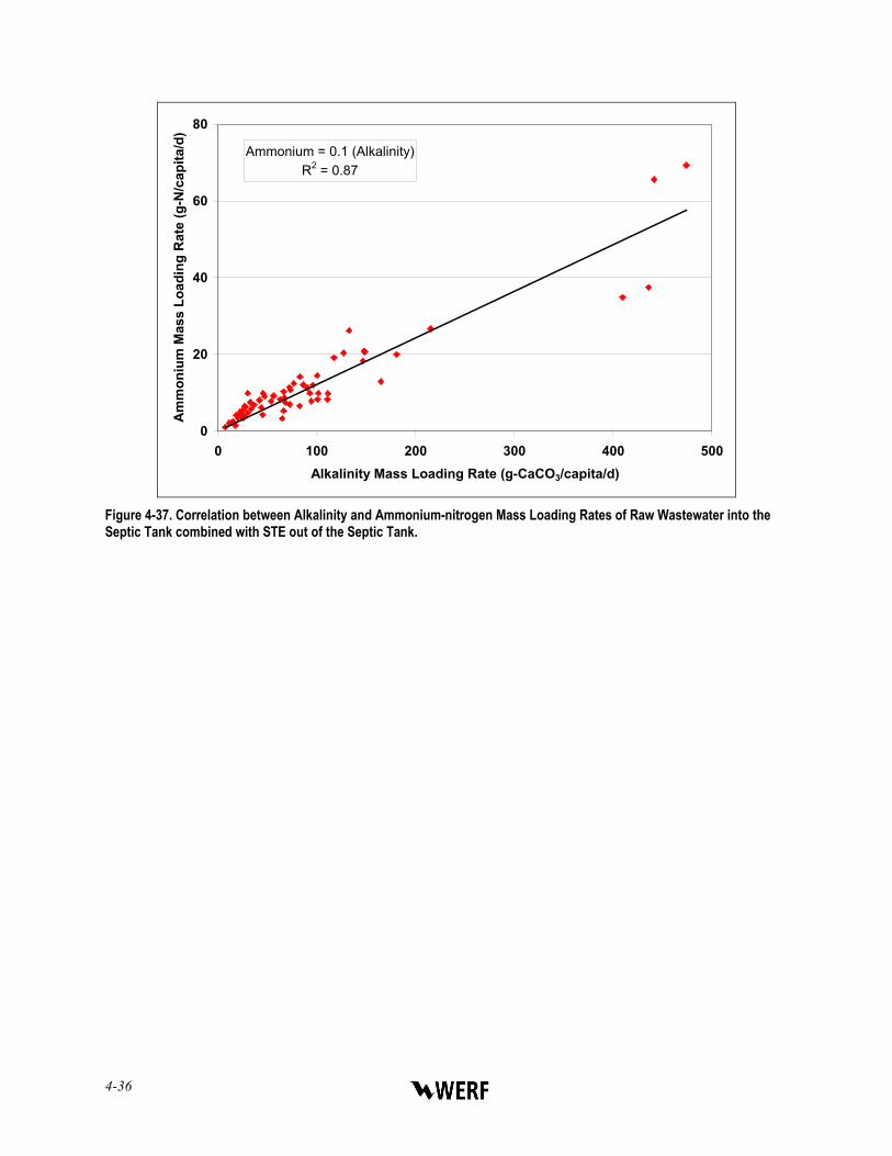
4-36
Ammonium = 0.1 (Alkalinity)R2 = 0.87
0
20
40
60
80
0 100 200 300 400 500Alkalinity Mass Loading Rate (g-CaCO3/capita/d)
Am
mon
ium
Mas
s Lo
adin
g R
ate
(g-N
/cap
ita/d
)
Figure 4-37. Correlation between Alkalinity and Ammonium-nitrogen Mass Loading Rates of Raw Wastewater into the Septic Tank combined with STE out of the Septic Tank.
Influent Constituent Characteristics of the Modern Waste Stream from Single Sources 5-1
CHAPTER 5.0
SUMMARY AND CONCLUSIONS 5.1 Summary
Decentralized wastewater management involving OWS has been recognized as a necessary and appropriate component of a sustainable wastewater infrastructure. Increasing uses of alternative OWS rely on additional treatment of the STE prior to discharge to the environment in sensitive areas or may eliminate use of a septic tank altogether. In addition, waste streams to be treated by OWS have changed during recent years due to changing lifestyles including increasing use of personal care and home cleaning products and lower water use due to water conservation efforts. While much research has been done to understand the composition of STE and its treatment in the soil or with engineered treatment units, limited information on raw wastewater is available. Data reported are often of different quality or type, limiting the usefulness of the information. Furthermore, scientific understanding has not been fully or clearly documented and thus not widely available to those working in the OWS field.
The overall goal of this research project was to characterize the extent of conventional constituents, microbial constituents, and organic wastewater contaminants in single source OWS raw wastewater and STE to aid OWS system design and management. The first phase of this research project was to conduct a thorough literature review to assess the current status of knowledge related to the composition of single source raw wastewater, identify key parameters affecting wastewater composition, and identify information gaps in the current knowledge. The literature review results can be found in Lowe et al., 2007 and the associated database (www.ndwrcdp.org/publications). Based on the findings of the literature review, the second phase of the research project was initiated to characterize the composition of residential single source raw wastewaters and STE.
Field investigations were conducted quarterly (fall, winter, spring, and summer) at a total of 17 sites from three regions (Colorado, Florida, and Minnesota) within the U.S. to ensure that the results and information gained had broad applicability to the management and design of OWS. Flow-weighted 24-hour composite samples were collected from the raw wastewater and STE. A tiered monitoring approach was utilized focusing on conventional constituents, microbial constituents, and organic chemicals. Tier 1 parameters were monitored at all sites and included pH, alkalinity, solids (TS and TSS), organic carbon (cBOD5, COD, and TOC/DOC), nutrients (total nitrogen, ammonium-nitrogen, nitrate-nitrogen, and total phosphorous), and fecal coliform bacteria. Tier 2 parameters were monitored at 50% of the sites and included E. coli, coliphage, and oil and grease. Tier 3 included organic trace chemicals monitored at 20% of the sites. In addition, daily and weekly variability within the raw wastewater and STE were monitored.
All households monitored during this project had OWS that were <20 years old (most were <10 years) with concrete chambered septic tanks between ~4,000 to 5,700 L. One site had two ~3000 L, non-chambered tanks and one site had two ~5700 L tanks serving an eight-unit apartment building. Households had two to six occupants ranging in age from small children to seniors (one site served an eight-unit apartment building with 18 occupants). Each household was given a detailed survey that included questions on water use, personal care products and pharmaceuticals used on a regular basis, septic system specifics (size, age, last pump, etc.), and
5-2
general household questions such as occupancy, number of bedrooms, use of garbage disposal and water softener.
The results were complied into spreadsheets and descriptive statistics (i.e., average, median, minimum, maximum, and standard deviation) and ANOVA tests were conducted. Data was evaluated by combining all the data together by waste stream (raw wastewater and STE) to identify general trends. Further data analyses included separating the data by regional location, season, and age of occupants. Graphical tools included preparation of CFDs, box and whisker plots, and individual parameter correlations.
5.2 Conclusions This report provides the findings from a comprehensive field monitoring program in
various formats to enable OWS designers and decision makers the ability to utilize the data in a number of ways. Most importantly, the reported data formats allow each individual data user to select representative constituent values with an understanding of the limitations of the data and potential uncertainty (i.e., negative or positive biases). In some cases, a median value may be of most interest, in some cases more specific values may be of interest, while in some cases an estimate may be warranted in the absence of data. Based on these findings, the following conclusions have been made:
♦ The median indoor water use was 171 L//d (n=64) (45.2 gpcd) which is 25% lower than previous studies conducted nearly 10 years ago (229 L/capita/d [60.5 gpcd], Mayer 1999).
♦ The range of Tier 1, Tier 2, and Tier 3 constituent concentrations was higher for raw wastewater compared to STE.
♦ An increase in alkalinity and ammonium-nitrogen concentrations from the raw wastewater to the STE was observed at all sites in each region and during each sampling event.
♦ A decrease in TS, TSS, cBOD5, COD, TOC, DOC, nitrate-nitrogen, and oil and grease from the raw wastewater to the STE was observed at all sites in each region and during each sampling event.
♦ The concentrations of consumer product chemicals ranged over three orders of magnitude. Caffeine, ethylenediaminetetraacetic acid (EDTA), 4-nonylphenolmonoethoxylate (NP1EO) and triclosan were detected in all STE samples.
♦ Of the pharmaceutical residues, pesticides, and flame retardants analyzed for, only ibuprofen, naproxen, and salicylic acid were detected in raw wastewater and STE.
♦ Significant (alpha = 0.05) regional variations in concentrations were observed for: o pH and alkalinity in raw wastewater, and
o pH, alkalinity, TS, cBOD5, COD, TOC, DOC, nitrate-nitrogen, and E. coli in STE.
♦ Significant (alpha = 0.05) variations due to the age of the household occupants (either over 65 or under 65) were observed for:
o water use,

Influent Constituent Characteristics of the Modern Waste Stream from Single Sources 5-3
o pH, alkalinity, and TS concentrations in raw wastewater, and
o alkalinity, TS, cBOD5, COD, TOC, DOC, total nitrogen, ammonium-nitrogen, nitrate-nitrogen, and total phosphorus concentrations in STE.
♦ No significant (alpha = 0.05) seasonal variations were observed for raw wastewater or STE concentrations.
♦ Weekly and daily variations were observed in the raw wastewater for all constituents (Tier 1, Tier 2, and Tier 3) with little variability observed in STE concentrations. The variations are attributed to the specific water use activities.
♦ Relationships between raw wastewater and STE concentrations were established for alkalinity and total phosphorus (R2 > 0.50). No relationship between raw wastewater and STE could be established for other Tier 1, Tier 2, or Tier 3 constituents. Relationships between different constituent concentrations in raw wastewater and STE combined were established for cBOD5 and COD, and TOC and DOC (R2 > 0.50). The complex differences between and interactions of system properties and processes remain unclear with insufficient replicates to determine concentration relationships.
♦ Mass loading rates for constituents from raw wastewater into the septic tank and from STE out of the septic tank were determined.
o Regional differences in mass loading rates were observed.
o Differences in mass loading rates attributed to the age of the occupants were observed.
o Relationships between raw wastewater and STE mass loading rates were established for cBOD5, COD, total nitrogen, and total phosphorus (R2 > 0.50).
o Relationships between different constituent mass loading rates of raw wastewater into the septic tanks combined with STE out of the septic tank were established for cBOD5 and COD, TOC and DOC, alkalinity and ammonium-nitrogen (R2 > 0.50).

5-4

Influent Constituent Characteristics of the Modern Waste Stream from Single Sources
A-1
APPENDIX A
RESIDENTIAL EVALUATION SURVEY

A-2
Name: ___________________________________ Date: ____________________ Time: ________________
Street Address: ____________________________ City: _______________________________
State: ____________________________________ Zip Code: ________________________________________
Mailing Address (if different from above):___________________________________________________________
Daytime Phone (Work or Cell): _______________ PM phone (Home or Cell): __________________________
Parcel #: _________________________________ Designer: ________________________________________
Installer: _________________________________ City : ___________________ State : ________________
Home/Residents
1. Is this your first home with an on-site wastewater treatment system? YES / NO
2. Did you receive any septic system user information? YES / NO
3. Did you receive the as-built drawing for the system? YES / NO
4. Any additions to the home since built?
Bedrooms ___________________________ Bathrooms ______________________________________
Other __________________________________________________________________________________
5. Type of use: Permanent / Seasonal If seasonal, number of months used __________________
a. Number of people living in the home: Adults (18-65): ___ M ___F
Seniors (>65): ___M ___F
Children (<13): ___ M ___F
Teenagers (13-17): ___ M ___F
b. Guests (Approximate number and frequency) _____________________________________________
c. Number of bedrooms: _____________ Number of bathrooms: ____________________________
d. Number of pets: Dogs______ Cats______ Number of pet baths per month: _____
6. Number of showers per week: _____ Number of baths per week: _____
7. Water supply: Private well / Centralized system / Other supply _______________________________
8. Do you have an in-home business? YES / NO
If “yes”, what type? ______________________________________________________________________
9. Is any resident using long term prescription drugs or antibiotics? YES / NO
If “yes”, what type? ______________________________________________________________________
_______________________________________________________________________________________
10. Please give the brand names of products used:
a. Shampoos_______________________________ Frequency __________________________
b. Toothpaste ______________________________ Frequency __________________________
c. Lotions _________________________________ Frequency __________________________
d. Body Soaps ______________________________ Frequency __________________________
e. Hand Soap ______________________________ Antibacterial? YES / NO
f. Non-prescription drugs used ____________________________________________________________
_________________________________________________ Frequency __________________________

Influent Constituent Characteristics of the Modern Waste Stream from Single Sources
A-3
11. Do you use septic system additives? YES / NO
If “yes”, what products? _________________________ Frequency: _________________________
Appliances and Cleaning Products
12. Home equipped with water conserving fixtures/appliances? YES / NO
Some/All? ________________________ List: __________________________________________
13. Garbage disposal? YES / NO Use: __________ times/day __________ times/week
14. Dishwasher used? YES / NO Use: __________ times/day __________ times/week
Dishwashing detergent used ____________________________
15. Laundry: Maximum __________ loads per day Consecutive loads: YES / NO
Total ______________ loads/week
a. Brand of laundry detergents used? _______________________________________ (powder / liquid)
b. Bleach used? YES / NO (powder / liquid) Use: _________ cups/load ________ loads/week
c. Hot or cold water used? _____________________________________________________________
d. Liquid fabric softener used? YES / NO
16. Whirlpool tub/Multi-head shower? YES / NO Use: _________ times/day ________ times/week
Approximate gallons per use ________________ For Shower, GPM __________________________
17. Is a drain cleaner used? YES / NO Type: ____________________________________
Frequency of use: ____________________________________________________________________
18. Number of rolls of toilet paper used per week? _________________________________________________
19. Toilet cleaning product brand? __________________ Cleanings/month ___________________________
Continuous cleaner used in toilet tank? YES / NO Brand/Type: _______________________________
20. Please list commonly used cleaning supplies:
Shower ________________________________ Kitchen ___________________________________
Floors _________________________________ Other: ____________________________________
21. Please list any antibacterial products: _________________________________________________________
22. Water treatment device(s): YES / NO
a. Is a water softener used? YES / NO
b. Reverse osmosis? YES / NO
c. Backwashing Water Filter (iron, sediment, etc)? YES / NO
d. Other Water Treatment Devices: _________________________________________________________
e. Record of System’s Service/History of any Problems _________________________________________
____________________________________________________________________________________
23. Air conditioner unit(s)? YES / NO Condensate drains to: _________________________________
24. Commercial ice machine? YES / NO Condensate drains to: _________________________________
25. Footing drains or basement sump pumps connected into the system? YES / NO
System (completed by O&M service provider or homeowner if no service provider)
26. Type of pretreatment system: Septic tank ATU Media filter Constructed wetland
a. Specific type of system _________________________________________________________________

A-4
b. Make and Model ______________________________________________________________________
27. How old is the system? ________ (years) Date of last pump out: ________________________________
28. Has the system ever backed up? YES / NO
29. Have the baffles ever been plugged? YES / NO
30. Effluent screen in septic tank outlet? YES / NO
31. Has effluent screen ever plugged? YES / NO Date(s): _____________________
32. Has the system ever been repaired? YES / NO
Record of System’s Service _________________________________________________________________
________________________________________________________________________________________
33. Has effluent ever surfaced? YES / NO
34. Has the alarm ever sounded? YES / NO
35. Soil type – at drainfield depth or lower: _______________________________________________________
36. Type of distribution/dispersal system: Gravity Trench Pressure dose Mound
Drip Spray Other: _____________________________________________________________
37. Control system: Demand / Timed
38. Design rate for system: ____________ (GPD)
39. Septic tank size: _________________ (gallons) Pump tank: ________________ (gallons)
40. Sludge levels in septic tank: 1st compartment accumulation _________ Floating materials _____________
2nd compartment accumulation _________ Floating materials _____________
41. Sludge level in pump tank: Accumulated _______________________ Floating materials _____________
42. Is the pump working? YES / NO
43. Duration of pump cycle: ____________ (minutes) Pump drawdown: ____________________________
Water Use
Actual indoor water use (GPD): Average: __________ High: __________ Low: __________
Reading this data from: ________ cycle counter
________ hour meter on pump
________ water meter
________ other
Actual outdoor water use (GPD): Average: __________ High: __________ Low: __________
Reading this data from: ________ cycle counter
________ hour meter on pump
________ water meter
________ other
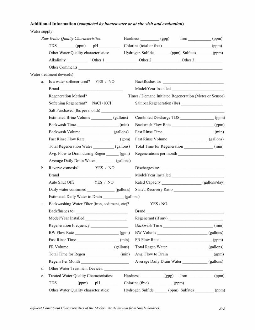
Influent Constituent Characteristics of the Modern Waste Stream from Single Sources
A-5
Additional Information (completed by homeowner or at site visit and evaluation) Water supply:
Raw Water Quality Characteristics: Hardness _________ (gpg) Iron ___________ (ppm)
TDS ________ (ppm) pH __________ Chlorine (total or free) _______________________ (ppm)
Other Water Quality characteristics: Hydrogen Sulfide _______ (ppm) Sulfates _______ (ppm)
Alkalinity __________ Other 1 _______________ Other 2 _____________ Other 3 _____________
Other Comments _____________________________________________________________________
Water treatment device(s):
a. Is a water softener used? YES / NO Backflushes to: _____________________________
Brand ______________________________ Model/Year Installed _________________________
Regeneration Method? Timer / Demand Initiated Regeneration (Meter or Sensor)
Softening Regenerant? NaCl / KCl Salt per Regeneration (lbs) ____________________
Salt Purchased (lbs per month) ___________________________________________________________
Estimated Brine Volume __________ (gallons) Combined Discharge TDS ________________ (ppm)
Backwash Time ____________________ (min) Backwash Flow Rate ____________________ (gpm)
Backwash Volume _______________ (gallons) Fast Rinse Time ________________________ (min)
Fast Rinse Flow Rate ________________ (gpm) Fast Rinse Volume ___________________ (gallons)
Total Regeneration Water __________ (gallons) Total Time for Regeneration ______________ (min)
Avg. Flow to Drain during Regen ______ (gpm) Regenerations per month ______________________
Average Daily Drain Water _________ (gallons)
b. Reverse osmosis? YES / NO Discharges to: ______________________________
Brand __________________________________ Model/Year Installed _________________________
Auto Shut Off? YES / NO Rated Capacity ___________________ (gallons/day)
Daily water consumed _____________ (gallons) Stated Recovery Ratio ________________________
Estimated Daily Water to Drain __________ (gallons)
c. Backwashing Water Filter (iron, sediment, etc)? YES / NO
Backflushes to: _________________________ Brand _____________________________________
Model/Year Installed ____________________ Regenerant (if any) __________________________
Regeneration Frequency __________________ Backwash Time ________________________ (min)
BW Flow Rate _____________________ (gpm) BW Volume ________________________ (gallons)
Fast Rinse Time ____________________ (min) FR Flow Rate _________________________ (gpm)
FR Volume _____________________ (gallons) Total Regen Water ___________________ (gallons)
Total Time for Regen ________________ (min) Avg. Flow to Drain _____________________ (gpm)
Regens Per Month _______________________ Average Daily Drain Water ____________ (gallons)
d. Other Water Treatment Devices: _________________________________________________________
e. Treated Water Quality Characteristics: Hardness ___________ (gpg) Iron ____________ (ppm)
TDS _________ (ppm) pH ________ Chlorine (free) ___________ (ppm)
Other Water Quality characteristics: Hydrogen Sulfide ______ (ppm) Sulfates _________ (ppm)

A-6
Alkalinity ___________ Other 1 ______________ Other 2 ____________ Other 3 _______________
Other Comments ______________________________________________________________________

Influent Characteristics of the Modern Waste Stream A-7
Site Sketch (Sketch the system or attach record of construction (as-built))
Scale 1” = ________ feet
Additional Notes:

A-8
Influent Constituent Characteristics of the Modern Waste Stream from Single Sources
B-1
APPENDIX B
TIER 1: CONVENTIONAL CONSTITUENTS

B-2
B.1 Water Use
0
20
40
60
80
100
0 200 400 600 800 1,000Water Use (L/capita/d)
Cum
ulat
ive
Freq
uenc
y (%
)
All Sites (n=64)
Lit Review (n=30)
Figure B-1. Indoor Water Use.
Table B-1. Descriptive Statistics for Water Use.
Water Use L/capita/d Mean SD Median Min Max IQR n All Sites 207 143 171 28 765 116-252 64 By Region Colorado 234 207 154 63 765 98-254 20 Florida 184 103 171 28 460 109-226 24 Minnesota 207 98 173 89 405 137-235 20 By Season Fall 231 188 177 28 731 108-351 16 Winter 182 61 190 99 281 120-229 15 Spring 234 177 171 64 765 133-284 16 Summer 171 108 148 54 475 97-227 17 By Age <65 148 78 137 28 405 87-196 40 >65 297 177 248 98 765 169-381 24 Literature Review 278 128 244 95 587 195-312 30
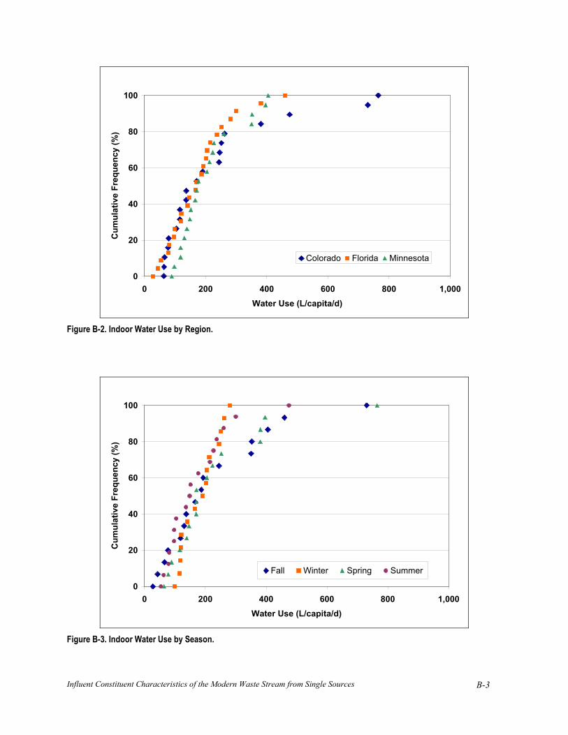
Influent Constituent Characteristics of the Modern Waste Stream from Single Sources
B-3
0
20
40
60
80
100
0 200 400 600 800 1,000Water Use (L/capita/d)
Cum
ulat
ive
Freq
uenc
y (%
)
Colorado Florida Minnesota
Figure B-2. Indoor Water Use by Region.
0
20
40
60
80
100
0 200 400 600 800 1,000Water Use (L/capita/d)
Cum
ulat
ive
Freq
uenc
y (%
)
Fall Winter Spring Summer
Figure B-3. Indoor Water Use by Season.

B-4
0
20
40
60
80
100
0 200 400 600 800 1,000Water Use (L/capita/d)
Cum
ulat
ive
Freq
uenc
y (%
)
65> 65<
Figure B-4. Indoor Water Use by Age.
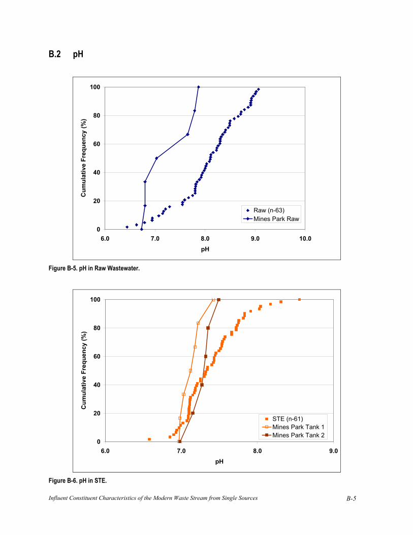
Influent Constituent Characteristics of the Modern Waste Stream from Single Sources
B-5
B.2 pH
0
20
40
60
80
100
6.0 7.0 8.0 9.0 10.0pH
Cum
ulat
ive
Freq
uenc
y (%
)
Raw (n-63)Mines Park Raw
Figure B-5. pH in Raw Wastewater.
0
20
40
60
80
100
6.0 7.0 8.0 9.0pH
Cum
ulat
ive
Freq
uenc
y (%
)
STE (n-61)Mines Park Tank 1Mines Park Tank 2
Figure B-6. pH in STE.
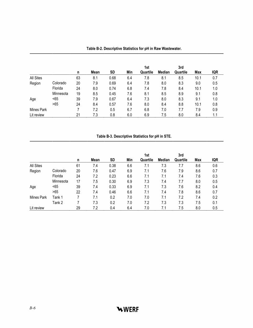
B-6
Table B-2. Descriptive Statistics for pH in Raw Wastewater.
n Mean SD Min 1st
Quartile Median 3rd
Quartile Max IQR All Sites 63 8.1 0.68 6.4 7.8 8.1 8.5 10.1 0.7 Region Colorado 20 7.9 0.69 6.4 7.8 8.0 8.3 9.0 0.5 Florida 24 8.0 0.74 6.8 7.4 7.8 8.4 10.1 1.0 Minnesota 19 8.5 0.45 7.6 8.1 8.5 8.9 9.1 0.8 Age <65 39 7.9 0.67 6.4 7.3 8.0 8.3 9.1 1.0 >65 24 8.4 0.57 7.6 8.0 8.4 8.8 10.1 0.8 Mines Park 7 7.2 0.5 6.7 6.8 7.0 7.7 7.9 0.9 Lit review 21 7.3 0.8 6.0 6.9 7.5 8.0 8.4 1.1
Table B-3. Descriptive Statistics for pH in STE.
n Mean SD Min 1st
Quartile Median 3rd
Quartile Max IQR All Sites 61 7.4 0.38 6.6 7.1 7.3 7.7 8.6 0.6 Region Colorado 20 7.6 0.47 6.9 7.1 7.6 7.9 8.6 0.7 Florida 24 7.2 0.23 6.6 7.1 7.1 7.4 7.6 0.3 Minnesota 17 7.5 0.30 6.9 7.3 7.4 7.7 8.0 0.5 Age <65 39 7.4 0.33 6.9 7.1 7.3 7.6 8.2 0.4 >65 22 7.4 0.46 6.6 7.1 7.4 7.8 8.6 0.7 Mines Park Tank 1 7 7.1 0.2 7.0 7.0 7.1 7.2 7.4 0.2 Tank 2 7 7.3 0.2 7.0 7.2 7.3 7.3 7.5 0.1 Lit review 29 7.2 0.4 6.4 7.0 7.1 7.5 8.0 0.5

Influent Constituent Characteristics of the Modern Waste Stream from Single Sources
B-7
6
7
8
9
10
Colorado Florida Minnesota
Region
pHIQR Boxplot
95% CI Mean Diamond
Outliers > 1.5 and < 3 IQR
Figure B-7. pH in Raw Wastewater by Region.
6
7
8
9
10
Colorado Florida Minnesota
Region
pH
IQR Boxplot
95% CI Mean Diamond
Outliers > 1.5 and < 3 IQR
Figure B-8. pH in STE by Region.
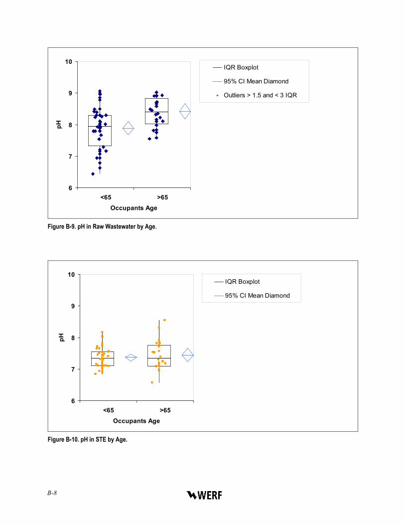
B-8
6
7
8
9
10
<65 >65Occupants Age
pHIQR Boxplot
95% CI Mean Diamond
Outliers > 1.5 and < 3 IQR
Figure B-9. pH in Raw Wastewater by Age.
6
7
8
9
10
<65 >65Occupants Age
pH
IQR Boxplot
95% CI Mean Diamond
Figure B-10. pH in STE by Age.

Influent Constituent Characteristics of the Modern Waste Stream from Single Sources
B-9
B.3 Alkalinity
0
20
40
60
80
100
0 200 400 600 800Alkalinity (mg-CaCO3/L)
Cum
ulat
ive
Freq
uenc
y (%
)
Raw (n=63)Mines Park Raw
Figure B-11. Alkalinity in Raw Wastewater.
0
20
40
60
80
100
0 200 400 600 800Alkalinity (mg-CaCO3/L)
Cum
ulat
ive
Freq
uenc
y (%
)
STE (n=61)Mines Park Tank 1Mines Park Tank 2
Figure B-12. Alkalinity in STE.

B-10
Table B-4. Descriptive Statistics for Alkalinity in Raw Wastewater.
n Mean SD Min 1st
Quartile Median 3rd
Quartile Max IQR All Sites 63 276 142 65 155 260 397 575 242 Region Colorado 20 184 118 65 99 145 230 484 130 Florida 24 252 116 95 159 267 322 568 163 Minnesota 19 405 99 226 337 414 480 575 143 Season Fall 16 270 128 81 172 268 353 575 181 Winter 15 260 160 65 104 258 383 568 278 Spring 16 281 137 103 152 268 426 484 274 Summer 16 293 153 92 159 265 441 526 282 Age <65 39 244 148 65 123 188 375 575 253 >65 24 330 115 164 237 313 440 568 203 Mines Park 7 70 24 50 53 56 85 106 32 Lit Review not reported
Table B-5. Descriptive Statistics for Alkalinity in STE.
n Mean SD Min 1st
Quartile Median 3rd
Quartile Max IQR All Sites 61 410 132 172 292 411 494 862 202 Region Colorado 20 366 175 172 235 333 397 862 163 Florida 24 385 96 252 275 392 467 543 192 Minnesota 17 497 65 376 464 494 541 617 77 Season Fall 15 397 128 194 272 411 492 605 220 Winter 14 400 134 217 260 390 494 620 234 Spring 16 399 110 172 308 389 495 570 187 Summer 16 442 159 232 310 445 516 862 206 Age <65 39 364 117 172 258 352 480 556 222 >65 22 490 121 353 390 467 573 862 183 Mines Park Tank 1 7 223 55 162 185 212 259 302 74 Tank 2 7 204 58 146 157 193 248 282 91 Lit Review 9 503 198 316 374 433 528 946 154

Influent Constituent Characteristics of the Modern Waste Stream from Single Sources
B-11
0
200
400
600
800
Colorado Florida Minnesota
Region
Alk
alin
ity (m
g-C
aCO
3/L)
IQR Boxplot
95% CI Mean Diamond
Outliers > 1.5 and < 3 IQR
Figure B-13. Alkalinity in Raw Wastewater by Region.
0
200
400
600
800
Colorado Florida Minnesota
Region
Alk
alin
ity (m
g-C
aCO
3/L)
IQR Boxplot
95% CI Mean Diamond
Outliers > 1.5 and < 3 IQR
Figure B-14. Alkalinity in STE by Region.

B-12
0
200
400
600
800
Fall Winter Spring SummerSeason
Alk
alin
ity (m
g-C
aCO
3/L)
Outlier Boxplot
95% CI Mean Diamond
Figure B-15. Alkalinity in Raw Wastewater by Season.
0
200
400
600
800
Fall Winter Spring SummerSeason
Alk
alin
ity (m
g-C
aCO
3/L)
Outlier Boxplot
95% CI Mean Diamond
Outliers > 1.5 and < 3 IQR
Figure B-16. Alkalinity in STE by Season.
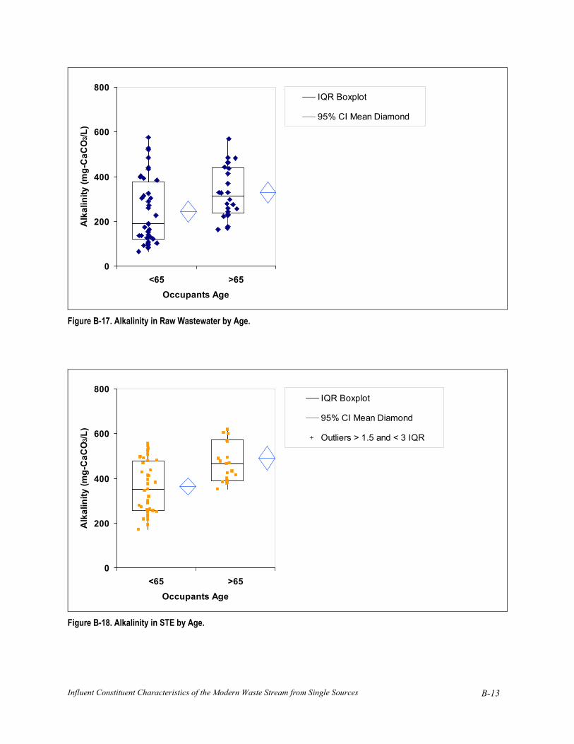
Influent Constituent Characteristics of the Modern Waste Stream from Single Sources
B-13
0
200
400
600
800
<65 >65Occupants Age
Alk
alin
ity (m
g-C
aCO
3/L)
IQR Boxplot
95% CI Mean Diamond
Figure B-17. Alkalinity in Raw Wastewater by Age.
0
200
400
600
800
<65 >65Occupants Age
Alk
alin
ity (m
g-C
aCO
3/L)
IQR Boxplot
95% CI Mean Diamond
Outliers > 1.5 and < 3 IQR
Figure B-18. Alkalinity in STE by Age.
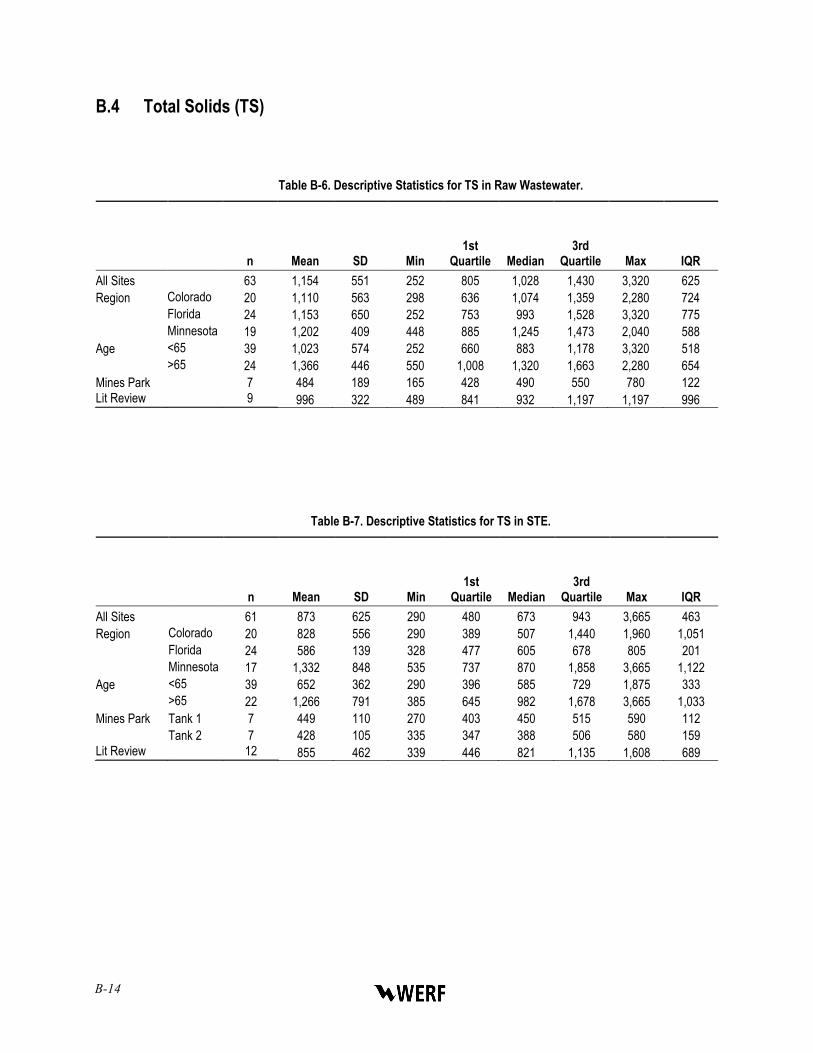
B-14
B.4 Total Solids (TS)
Table B-6. Descriptive Statistics for TS in Raw Wastewater.
n Mean SD Min 1st
Quartile Median 3rd
Quartile Max IQR All Sites 63 1,154 551 252 805 1,028 1,430 3,320 625 Region Colorado 20 1,110 563 298 636 1,074 1,359 2,280 724 Florida 24 1,153 650 252 753 993 1,528 3,320 775 Minnesota 19 1,202 409 448 885 1,245 1,473 2,040 588 Age <65 39 1,023 574 252 660 883 1,178 3,320 518 >65 24 1,366 446 550 1,008 1,320 1,663 2,280 654 Mines Park 7 484 189 165 428 490 550 780 122 Lit Review 9 996 322 489 841 932 1,197 1,197 996
Table B-7. Descriptive Statistics for TS in STE.
n Mean SD Min 1st
Quartile Median 3rd
Quartile Max IQR All Sites 61 873 625 290 480 673 943 3,665 463 Region Colorado 20 828 556 290 389 507 1,440 1,960 1,051 Florida 24 586 139 328 477 605 678 805 201 Minnesota 17 1,332 848 535 737 870 1,858 3,665 1,122 Age <65 39 652 362 290 396 585 729 1,875 333 >65 22 1,266 791 385 645 982 1,678 3,665 1,033 Mines Park Tank 1 7 449 110 270 403 450 515 590 112 Tank 2 7 428 105 335 347 388 506 580 159 Lit Review 12 855 462 339 446 821 1,135 1,608 689
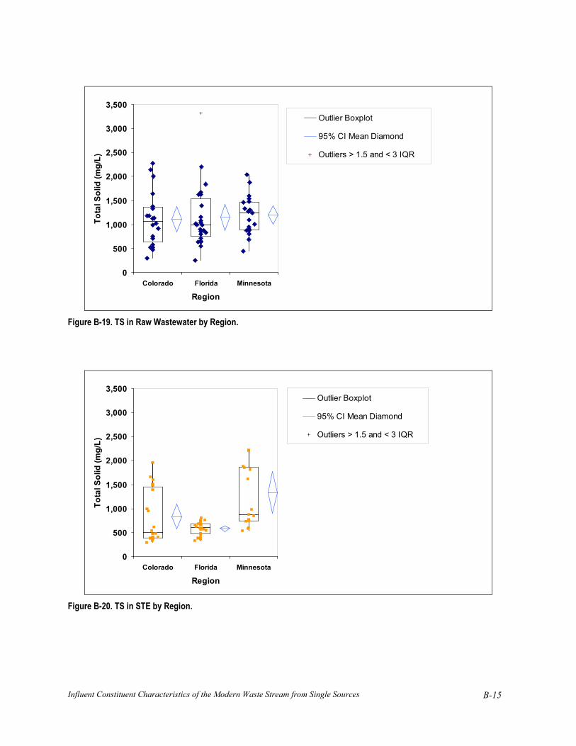
Influent Constituent Characteristics of the Modern Waste Stream from Single Sources
B-15
0
500
1,000
1,500
2,000
2,500
3,000
3,500
Colorado Florida Minnesota
Region
Tota
l Sol
id (m
g/L)
Outlier Boxplot
95% CI Mean Diamond
Outliers > 1.5 and < 3 IQR
Figure B-19. TS in Raw Wastewater by Region.
0
500
1,000
1,500
2,000
2,500
3,000
3,500
Colorado Florida Minnesota
Region
Tota
l Sol
id (m
g/L)
Outlier Boxplot
95% CI Mean Diamond
Outliers > 1.5 and < 3 IQR
Figure B-20. TS in STE by Region.
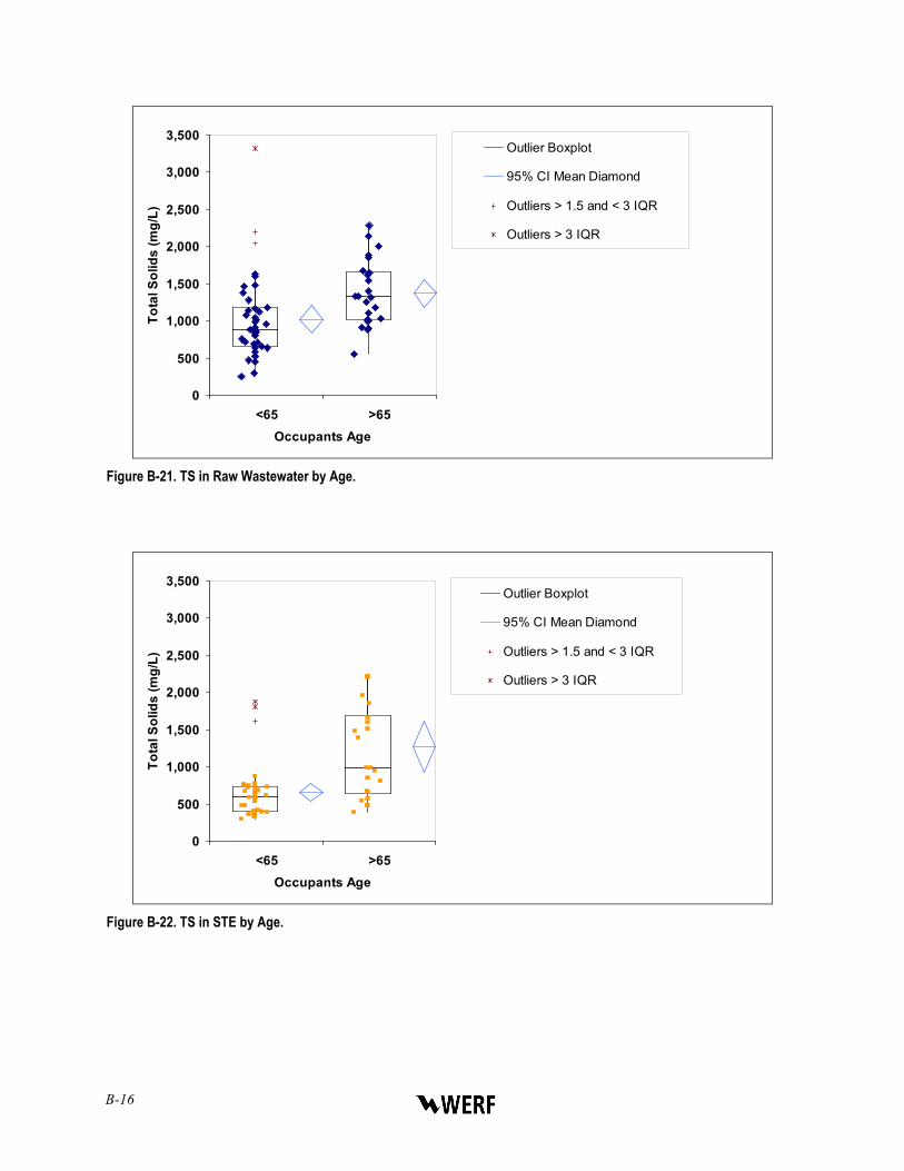
B-16
0
500
1,000
1,500
2,000
2,500
3,000
3,500
<65 >65Occupants Age
Tota
l Sol
ids
(mg/
L)Outlier Boxplot
95% CI Mean Diamond
Outliers > 1.5 and < 3 IQR
Outliers > 3 IQR
Figure B-21. TS in Raw Wastewater by Age.
0
500
1,000
1,500
2,000
2,500
3,000
3,500
<65 >65Occupants Age
Tota
l Sol
ids
(mg/
L)
Outlier Boxplot
95% CI Mean Diamond
Outliers > 1.5 and < 3 IQR
Outliers > 3 IQR
Figure B-22. TS in STE by Age.
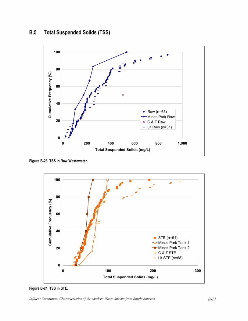
Influent Constituent Characteristics of the Modern Waste Stream from Single Sources
B-17
B.5 Total Suspended Solids (TSS)
0
20
40
60
80
100
0 200 400 600 800 1,000Total Suspended Solids (mg/L)
Cum
ulat
ive
Freq
uenc
y (%
)
Raw (n=63)Mines Park RawC & T RawLit Raw (n=31)
Figure B-23. TSS in Raw Wastewater.
0
20
40
60
80
100
0 100 200 300Total Suspended Solids (mg/L)
Cum
ulat
ive
Freq
uenc
y (%
)
STE (n=61)Mines Park Tank 1Mines Park Tank 2C & T STELit STE (n=68)
Figure B-24. TSS in STE.

B-18
Table B-8. Descriptive Statistics for TSS in Raw Wastewater.
n Mean SD Min 1st
Quartile Median 3rd
Quartile Max IQR All Sites 63 328 285 22 159 232 395 1,690 236 Region Colorado 20 305 204 67 166 223 408 740 242 Florida 24 373 396 22 109 218 472 1,690 363 Minnesota 19 296 174 82 170 280 379 822 209 Age <65 39 308 289 22 123 221 392 1,690 270 >65 24 362 280 82 170 260 399 1,190 229 Mines Park 7 203 164 49 94 173 238 534 144 Lit Review 30 402 461 18 174 280 396 2,233 402
Table B-9. Descriptive Statistics for TSS in STE.
n Mean SD Min 1st
Quartile Median 3rd
Quartile Max IQR All Sites 61 69 32 28 49 61 84 192 35 Region Colorado 20 72 39 31 47 58 86 192 39 Florida 24 63 26 28 45 56 78 132 33 Minnesota 17 75 32 29 50 69 97 128 46 Age <65 39 65 32 28 43 55 77 192 34 >65 22 77 32 28 51 70 93 150 42 Mines Park Tank 1 7 74 21 35 67 74 87 99 20 Tank 2 7 50 13 29 43 53 56 66 13 Lit Review 93 81 60 20 44 61 92 276 48
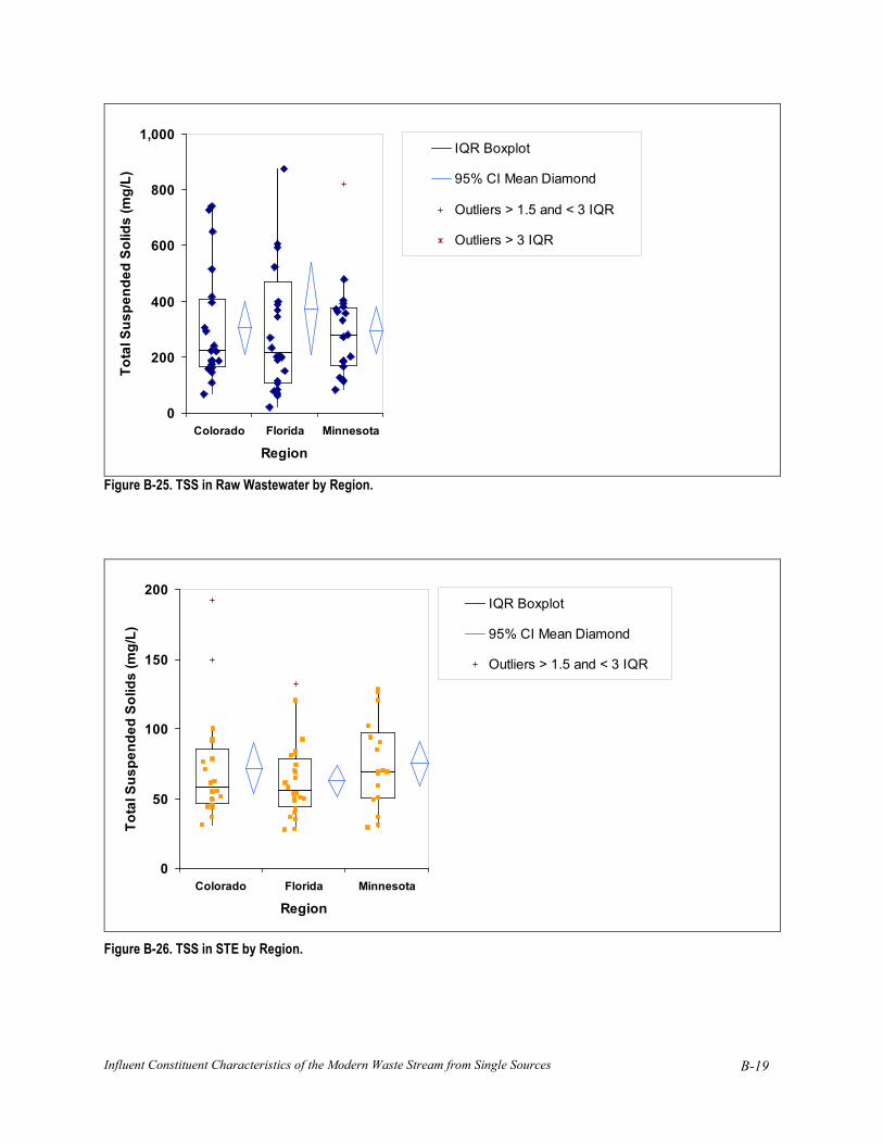
Influent Constituent Characteristics of the Modern Waste Stream from Single Sources
B-19
0
200
400
600
800
1,000
Colorado Florida Minnesota
Region
Tota
l Sus
pend
ed S
olid
s (m
g/L)
IQR Boxplot
95% CI Mean Diamond
Outliers > 1.5 and < 3 IQR
Outliers > 3 IQR
Figure B-25. TSS in Raw Wastewater by Region.
0
50
100
150
200
Colorado Florida Minnesota
Region
Tota
l Sus
pend
ed S
olid
s (m
g/L)
IQR Boxplot
95% CI Mean Diamond
Outliers > 1.5 and < 3 IQR
Figure B-26. TSS in STE by Region.

B-20
0
200
400
600
800
1,000
<65 >65Occupants Age
Tota
l Sus
pend
ed S
olid
s (m
g/L)
IQR Boxplot
95% CI Mean Diamond
Outliers > 1.5 and < 3 IQR
Outliers > 3 IQR
Figure B-27. TSS in Raw Wastewater by Age.
0
50
100
150
200
<65 >65Occupants Age
Tota
l Sus
pend
ed S
olid
s (m
g/L)
IQR Boxplot
95% CI Mean Diamond
Outliers > 1.5 and < 3 IQR
Outliers > 3 IQR
Figure B-28. TSS in STE by Age.

Influent Constituent Characteristics of the Modern Waste Stream from Single Sources
B-21
B.6 cBOD5
0
20
40
60
80
100
0 200 400 600 800 1,000 1,200cBOD5 (mg/L)
Cum
ulat
ive
Freq
uenc
y (%
)
Raw (n=62)Mines Park Raw C & T Raw (1998)Lit Review Raw (n=29)
Figure B-29. cBOD5 in Raw Wastewater.
0
20
40
60
80
100
0 200 400 600 800 1,000cBOD5 (mg/L)
Cum
ulat
ive
Freq
uenc
y (%
)
STE (n=59)Mines Park Tank 1Mines Park Tank 2C & T STE (1998)Lit Review STE (n=92)
Figure B-30. cBOD5 in STE.

B-22
Table B-10. Descriptive Statistics for cBOD5 in Raw Wastewater.
cBOD5 mg/L
n Mean SD Min 1st
Quartile Median 3rd
Quartile Max IQR All Sites 62 443 213 112 294 420 568 1,101 275 By Region Colorado 20 489 206 112 389 472 604 912 254 Florida 23 455 207 136 262 427 615 841 361 Minnesota 19 381 224 118 262 320 421 1,101 177 By Season Fall 16 456 216 118 332 418 564 912 231 Winter 15 400 258 112 197 322 473 1,101 276 Spring 16 425 201 136 276 404 545 841 269 Summer 15 491 183 236 302 499 656 784 353 By Age <65 39 405 201 112 257 401 554 912 297 >65 23 508 222 188 390 433 686 1,101 296 Mines Park 6 329 130 180 243 303 400 533 157 Lit Review (as BOD5) 27 355 223 30 202 337 482 1,147 280
Table B-11. Descriptive Statistics for cBOD5 in STE.
cBOD5 mg/L
n Mean SD Min
1st Quartile Median
3rd Quartile Max IQR
All Sites 59 252 156 44 156 216 294 833 138 Region Colorado 20 324 181 74 225 274 329 833 128 Florida 23 206 137 44 129 182 228 718 102 Minnesota 16 228 118 82 149 188 270 545 131 Season Fall 15 282 172 44 174 258 356 680 182 Winter 14 283 178 74 180 208 383 718 202 Spring 16 222 78 77 158 243 285 313 127 Summer 14 222 182 88 151 165 236 833 86 Age <65 38 211 111 44 139 201 269 680 130 >65 21 326 196 125 193 258 424 833 230 Mines Park Tank 1 6 234 65 160 195 226 255 345 60 Tank 2 6 187 63 85 159 198 233 254 74 Lit Review 98 181 102 39 120 158 226 861 106

Influent Constituent Characteristics of the Modern Waste Stream from Single Sources
B-23
0
200
400
600
800
1,000
1,200
Colorado Florida Minnesota
Region
cBO
D5 (
mg/
L)
IQR Boxplot
95% CI Mean Diamond
Outliers > 1.5 and < 3 IQR
Outliers > 3 IQR
Figure B-31. cBOD5 in Raw Wastewater by Region.
0
200
400
600
800
1,000
Colorado Florida Minnesota
Region
cBO
D5 (
mg/
L)
IQR Boxplot
95% CI Mean Diamond
Outliers > 1.5 and < 3 IQR
Outliers > 3 IQR
Figure B-32. cBOD5 in STE by Region.

B-24
0
200
400
600
800
1,000
1,200
Fall Winter Spring SummerSeason
cBO
D5 (
mg/
L)
IQR Boxplot
95% CI Mean Diamond
Outliers > 1.5 and < 3 IQR
Figure B-33. cBOD5 in Raw Wastewater by Season.
0
200
400
600
800
1,000
Fall Winter Spring SummerSeason
cBO
D5 (
mg/
L)
IQR Boxplot
95% CI Mean Diamond
Outliers > 1.5 and < 3 IQR
Outliers > 3 IQR
Figure B-34. cBOD5 in Raw Wastewater by Season.
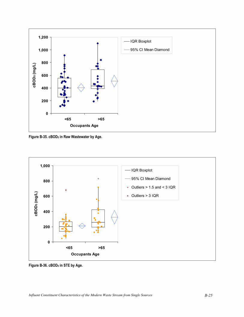
Influent Constituent Characteristics of the Modern Waste Stream from Single Sources
B-25
0
200
400
600
800
1,000
1,200
<65 >65Occupants Age
cBO
D5 (
mg/
L)
IQR Boxplot
95% CI Mean Diamond
Figure B-35. cBOD5 in Raw Wastewater by Age.
0
200
400
600
800
1,000
<65 >65Occupants Age
cBO
D5 (
mg/
L)
IQR Boxplot
95% CI Mean Diamond
Outliers > 1.5 and < 3 IQR
Outliers > 3 IQR
Figure B-36. cBOD5 in STE by Age.
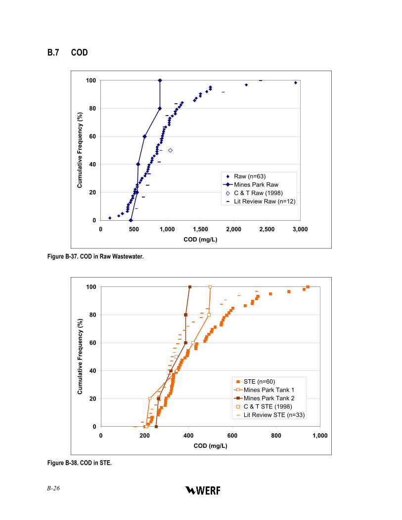
B-26
B.7 COD
0
20
40
60
80
100
0 500 1,000 1,500 2,000 2,500 3,000COD (mg/L)
Cum
ulat
ive
Freq
uenc
y (%
)
Raw (n=63)Mines Park RawC & T Raw (1998)Lit Review Raw (n=12)
Figure B-37. COD in Raw Wastewater.
0
20
40
60
80
100
0 200 400 600 800 1,000COD (mg/L)
Cum
ulat
ive
Freq
uenc
y (%
)
STE (n=60)Mines Park Tank 1Mines Park Tank 2C & T STE (1998)Lit Review STE (n=33)
Figure B-38. COD in STE.
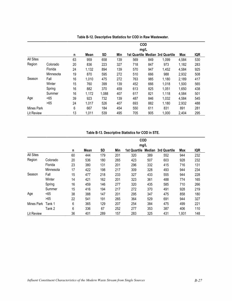
Influent Constituent Characteristics of the Modern Waste Stream from Single Sources
B-27
Table B-12. Descriptive Statistics for COD in Raw Wastewater.
COD mg/L
n Mean SD Min 1st Quartile Median 3rd Quartile Max IQR All Sites 63 959 658 139 569 849 1,099 4,584 530 Region Colorado 20 836 223 327 718 847 973 1,182 283 Florida 24 1,132 894 139 570 947 1,452 4,584 925 Minnesota 19 870 595 272 510 666 988 2,932 508 Season Fall 16 1,010 475 272 763 985 1,180 2,189 417 Winter 15 760 399 139 452 666 1,018 1,500 565 Spring 16 882 370 459 613 825 1,051 1,650 438 Summer 16 1,172 1,088 407 617 821 1,118 4,584 501 Age <65 39 923 732 139 487 846 1,032 4,584 545 >65 24 1,017 526 407 693 882 1,180 2,932 488 Mines Park 6 667 184 454 550 611 831 891 281 Lit Review 13 1,011 539 495 705 905 1,000 2,404 295
Table B-13. Descriptive Statistics for COD in STE.
COD mg/L
n Mean SD Min 1st Quartile Median 3rd Quartile Max IQR All Sites 60 444 179 201 320 389 552 944 232 Region Colorado 20 536 180 265 423 507 603 928 232 Florida 23 380 131 201 296 332 415 716 131 Minnesota 17 422 198 217 309 328 493 944 234 Season Fall 15 477 218 233 327 433 555 944 228 Winter 14 421 162 201 323 361 488 774 165 Spring 16 459 146 277 320 435 585 710 266 Summer 15 416 194 217 272 370 491 928 219 Age <65 38 388 147 201 295 347 475 858 180 >65 22 541 191 265 364 529 691 944 327 Mines Park Tank 1 6 365 129 207 254 384 475 499 221 Tank 2 6 336 67 252 277 353 387 406 110 Lit Review 36 401 289 157 283 325 431 1,931 148

B-28
0
500
1,000
1,500
2,000
2,500
3,000
Colorado Florida Minnesota
Region
CO
D (m
g/L)
IQR Boxplot
95% CI Mean Diamond
Outliers > 3 IQR
Figure B-39. COD in Raw Wastewater by Region.
0
200
400
600
800
1,000
Colorado Florida Minnesota
Region
CO
D (m
g/L)
IQR Boxplot
95% CI Mean Diamond
Outliers > 1.5 and < 3 IQR
Figure B-40. COD in STE by Region.
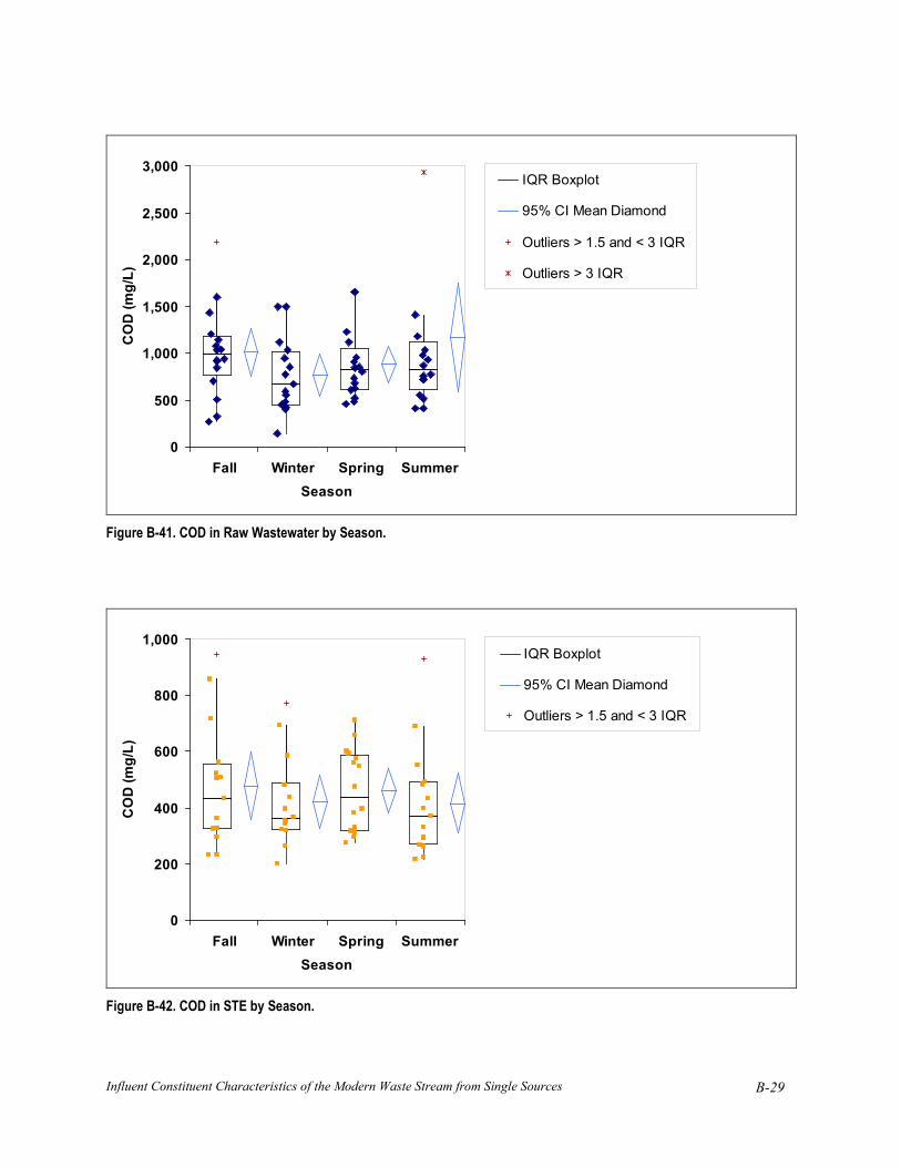
Influent Constituent Characteristics of the Modern Waste Stream from Single Sources
B-29
0
500
1,000
1,500
2,000
2,500
3,000
Fall Winter Spring SummerSeason
CO
D (m
g/L)
IQR Boxplot
95% CI Mean Diamond
Outliers > 1.5 and < 3 IQR
Outliers > 3 IQR
Figure B-41. COD in Raw Wastewater by Season.
0
200
400
600
800
1,000
Fall Winter Spring SummerSeason
CO
D (m
g/L)
IQR Boxplot
95% CI Mean Diamond
Outliers > 1.5 and < 3 IQR
Figure B-42. COD in STE by Season.

B-30
0
500
1,000
1,500
2,000
2,500
3,000
<65 >65Occupants Age
CO
D (m
g/L)
IQR Boxplot
95% CI Mean Diamond
Outliers > 1.5 and < 3 IQR
Outliers > 3 IQR
Figure B-43. COD in Raw Wastewater by Age.
0
200
400
600
800
1,000
<65 >65Occupants Age
CO
D (m
g/L)
IQR Boxplot
95% CI Mean Diamond
Outliers > 1.5 and < 3 IQR
Figure B-44. COD in STE by Age.
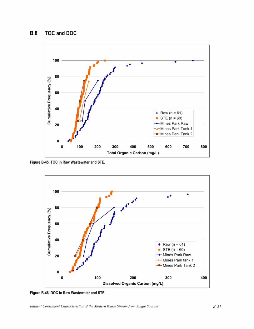
Influent Constituent Characteristics of the Modern Waste Stream from Single Sources
B-31
B.8 TOC and DOC
0
20
40
60
80
100
0 100 200 300 400 500 600 700 800Total Organic Carbon (mg/L)
Cum
ulat
ive
Freq
uenc
y (%
)
Raw (n = 61)STE (n = 60)Mines Park RawMines Park Tank 1Mines Park Tank 2
Figure B-45. TOC in Raw Wastewater and STE.
0
20
40
60
80
100
0 100 200 300 400Dissolved Organic Carbon (mg/L)
Cum
ulat
ive
Freq
uenc
y (%
)
Raw (n = 61)STE (n = 60)Mines Park RawMines Park tank 1Mines Park Tank 2
Figure B-46. DOC in Raw Wastewater and STE.

B-32
Table B-14. Descriptive Statistics for TOC in Raw Wastewater.
n Mean SD Min 1st
Quartile Median 3rd
Quartile Max IQR All Sites 63 204 123 35 133 184 234 738 101 Region Colorado 20 185 47 77 152 184 219 275 67 Florida 23 246 165 62 136 215 290 738 154 Minnesota 19 160 101 35 88 134 211 451 123 Age <65 39 204 140 35 125 166 236 738 111 >65 23 193 85 42 153 183 229 451 76 Mines Park 3 149 Lit Review not reported
Table B-15. Descriptive Statistics for TOC in STE.
n Mean SD Min 1st
Quartile Median 3rd
Quartile Max IQR All Sites 61 1110 40 50 81 105 133 243 52 Region Colorado 20 129 39 71 107 124 152 243 46 Florida 23 100 28 50 81 91 122 156 41 Minnesota 18 103 49 52 70 80 118 202 47 Age <65 40 102 39 50 76 92 122 243 46 >65 21 126 39 74 90 123 152 202 62 Mines Park Tank 1 3 124 Tank 2 3 104 Lit Review not reported

Influent Constituent Characteristics of the Modern Waste Stream from Single Sources
B-33
Table B-16. Descriptive Statistics for DOC in Raw Wastewater.
n Mean SD Min 1st
Quartile Median 3rd
Quartile Max IQR All Sites 63 139 1054 29 85 110 153 679 68 Region Colorado 20 123 49 31 88 119 152 207 65 Florida 24 173 147 45 97 138 182 679 86 Minnesota 19 108 72 29 74 88 114 355 40 Age <65 39 143 121 29 80 108 147 679 67 >65 24 127 68 31 86 109 157 355 71 Mines Park 4 99 Lit Review not reported
Table B-17. Descriptive Statistics for DOC in STE.
n Mean SD Min 1st
Quartile Median 3rd
Quartile Max IQR All Sites 61 74 30 22 52 66 95 140 43 Region Colorado 20 86 30 22 74 90 104 139 30 Florida 24 63 25 27 50 59 81 108 31 Minnesota 17 69 33 32 46 56 86 140 40 Age <65 39 65 27 27 44 60 89 139 45 >65 22 86 33 22 57 91 106 140 49 Mines Park Tank 1 4 71 Tank 2 4 71 Lit Review not reported

B-34
0
200
400
600
800
Colorado Florida Minnesota
Region
TOC
(mg/
L)
Figure B-47. TOC in Raw Wastewater by Region. Figure B-48. TOC in STE by Region.
0
200
400
600
800
Colorado Florida Minnesota
Region
DO
C (m
g/L)
Figure B-49. DOC in Raw Wastewater by Region. Figure B-50. DOC in STE by Region.
0
50
100
150
200
250
300
Colorado Florida Minnesota
Region
TOC
(mg/
L)
0
50
100
150
200
250
300
Colorado Florida Minnesota
Region
DO
C (m
g/L)

Influent Constituent Characteristics of the Modern Waste Stream from Single Sources
B-35
0
200
400
600
800
<65 >65Occupants Age
TOC
(mg/
L)
Figure B-51. TOC in Raw Wastewater by Age. Figure B-52. TOC in STE by Age.
0
200
400
600
800
<65 >65Occupants Age
DO
C (m
g/L)
Figure B-53. DOC in Raw Wastewater by Age. Figure B-54. DOC in STE by Age.
0
50
100
150
200
250
300
<65 >65Occupants Age
TOC
(mg/
L)
0
50
100
150
200
250
300
<65 >65Occupants Age
DO
C (m
g/L)

B-36
B.9 Total Nitrogen
0
20
40
60
80
100
0 50 100 150 200 250 300Total Nitrogen (mg-N/L)
Cum
ulat
ive
Freq
uenc
y (%
)
Raw (n=63)Mines Park RawC & T Raw (1998)Lit Review Raw (n=11)
Figure B-55. Total Nitrogen in Raw Wastewater.
0
20
40
60
80
100
0 20 40 60 80 100 120 140Total Nitrogen (mg-N/L)
Cum
ulat
ive
Freq
uenc
y (%
)
STE (n=61)Mines Park Tank 1Mines Park Tank 2C & T STE (1998)Lit Review STE (n=40)
Figure B-56. Total Nitrogen in STE.

Influent Constituent Characteristics of the Modern Waste Stream from Single Sources
B-37
Table B-18. Descriptive Statistics for Total Nitrogen in Raw Wastewater.
Total Nitrogen mg/L
n Mean SD Min 1st
Quartile Median 3rd
Quartile Max IQR All Sites 63 71 43 9 41 60 92 240 50 Region Colorado 20 63 35 9 43 59 77 148 34 Florida 24 73 50 11 36 71 90 240 54 Minnesota 19 76 43 10 42 57 124 150 82 Season Fall 16 68 52 10 29 51 116 155 87 Winter 15 63 28 22 38 60 81 120 44 Spring 16 67 33 9 48 70 85 139 37 Summer 16 83 56 23 44 70 119 240 75 Age <65 39 64 45 9 32 54 81 240 49 >65 24 82 39 23 52 76 110 155 58 Mines Park 6 46 13 24 41 47 52 63 11 Lit Review 11 87 45 44 62 63 120 189 58
Table B-19. Descriptive Statistics for Total Nitrogen in STE.
Total Nitrogen mg/L
n Mean SD Min 1st
Quartile Median 3rd
Quartile Max IQR All Sites 61 64 21 27 47 63 78 119 31 Region Colorado 20 69 26 27 50 71 87 119 38 Florida 24 61 14 38 47 65 72 86 25 Minnesota 17 62 25 30 46 52 82 118 36 Season Fall 15 62 26 27 42 59 74 118 32 Winter 14 70 22 42 51 71 80 119 29 Spring 16 57 18 27 44 58 70 89 26 Summer 16 68 20 38 51 67 81 109 30 Age <65 39 58 20 27 44 52 71 119 27 >65 22 74 20 27 61 75 86 118 25 Mines Park Tank 1 6 55 11 45 49 52 61 73 12 Tank 2 6 51 15 33 43 45 60 74 17 Lit Review 40 58 17 26 46 54 65 124 19

B-38
0
50
100
150
200
250
Colorado Florida Minnesota
Region
Tota
l Nitr
ogen
(mg-
N/L
)IQR Boxplot
95% CI Mean Diamond
Outliers > 1.5 and < 3 IQR
Figure B-57. Total Nitrogen in Raw Wastewater by Region.
0
50
100
150
200
Colorado Florida Minnesota
Region
Tota
l Nitr
ogen
(mg-
N/L
)
IQR Boxplot
95% CI Mean Diamond
Figure B-58. Total Nitrogen in STE by Region.
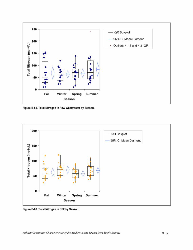
Influent Constituent Characteristics of the Modern Waste Stream from Single Sources
B-39
0
50
100
150
200
250
Fall Winter Spring SummerSeason
Tota
l Nitr
ogen
(mg-
N/L
)IQR Boxplot
95% CI Mean Diamond
Outliers > 1.5 and < 3 IQR
Figure B-59. Total Nitrogen in Raw Wastewater by Season.
0
50
100
150
200
Fall Winter Spring SummerSeason
Tota
l Nitr
ogen
(mg-
N/L
)
IQR Boxplot
95% CI Mean Diamond
Figure B-60. Total Nitrogen in STE by Season.
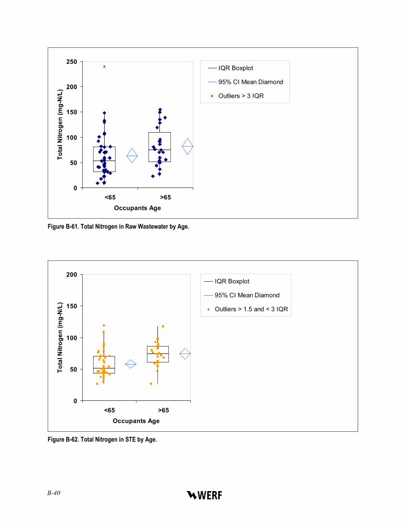
B-40
0
50
100
150
200
250
<65 >65Occupants Age
Tota
l Nitr
ogen
(mg-
N/L
)IQR Boxplot
95% CI Mean Diamond
Outliers > 3 IQR
Figure B-61. Total Nitrogen in Raw Wastewater by Age.
0
50
100
150
200
<65 >65Occupants Age
Tota
l Nitr
ogen
(mg-
N/L
)
IQR Boxplot
95% CI Mean Diamond
Outliers > 1.5 and < 3 IQR
Figure B-62. Total Nitrogen in STE by Age.

Influent Constituent Characteristics of the Modern Waste Stream from Single Sources
B-41
B.10 Ammonium-Nitrogen
0
20
40
60
80
100
0 20 40 60 80 100 120Ammonium-Nitrogen (mg-N/L)
Cum
ulat
ive
Freq
uenc
y (%
)
Raw (n=63)Mines Park RawC & T Raw (1998)Lit Review Raw (n=12)
Figure B-63. Ammonium-nitrogen in Raw Wastewater.
0
20
40
60
80
100
0 20 40 60 80 100 120Ammonium-Nitrogen (mg-N/L)
Cum
ulat
ive
Freq
uenc
y (%
)
STE (n=61)Mines Park Tank 1Mines Park Tank 2Lit Review STE (n=78)
Figure B-64. Ammonium-nitrogen in STE.
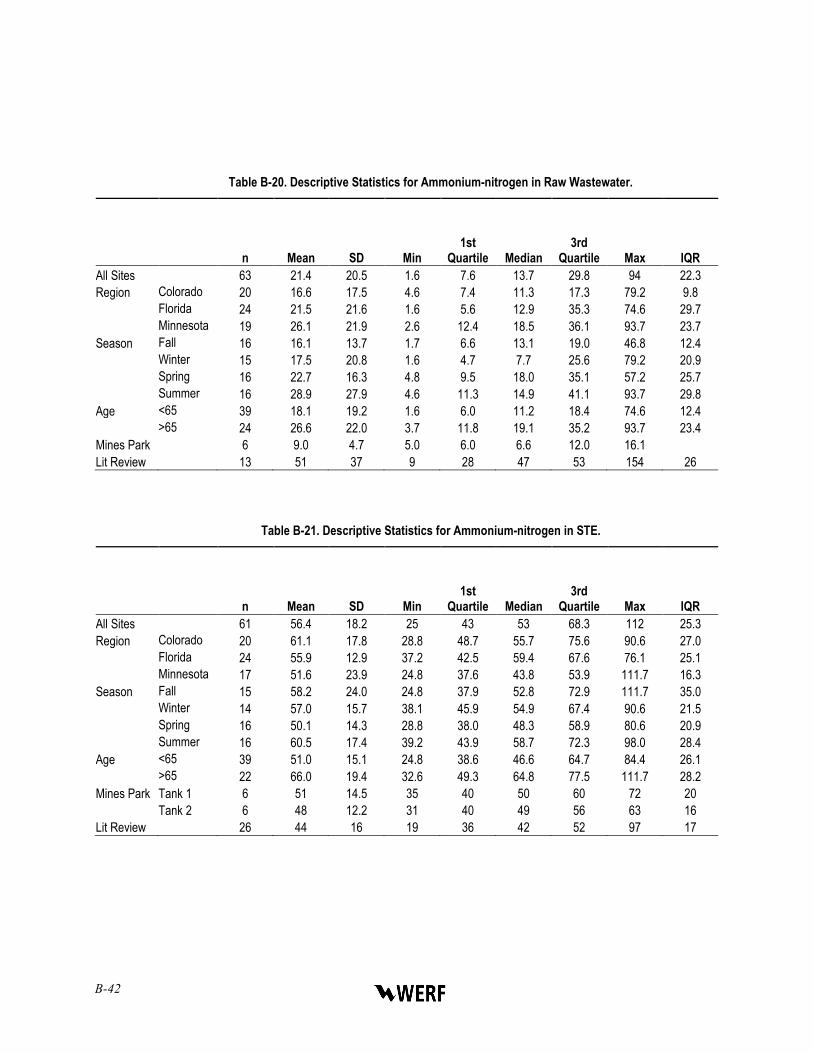
B-42
Table B-20. Descriptive Statistics for Ammonium-nitrogen in Raw Wastewater.
n Mean SD Min 1st
Quartile Median 3rd
Quartile Max IQR All Sites 63 21.4 20.5 1.6 7.6 13.7 29.8 94 22.3 Region Colorado 20 16.6 17.5 4.6 7.4 11.3 17.3 79.2 9.8 Florida 24 21.5 21.6 1.6 5.6 12.9 35.3 74.6 29.7 Minnesota 19 26.1 21.9 2.6 12.4 18.5 36.1 93.7 23.7 Season Fall 16 16.1 13.7 1.7 6.6 13.1 19.0 46.8 12.4 Winter 15 17.5 20.8 1.6 4.7 7.7 25.6 79.2 20.9 Spring 16 22.7 16.3 4.8 9.5 18.0 35.1 57.2 25.7 Summer 16 28.9 27.9 4.6 11.3 14.9 41.1 93.7 29.8 Age <65 39 18.1 19.2 1.6 6.0 11.2 18.4 74.6 12.4 >65 24 26.6 22.0 3.7 11.8 19.1 35.2 93.7 23.4 Mines Park 6 9.0 4.7 5.0 6.0 6.6 12.0 16.1 Lit Review 13 51 37 9 28 47 53 154 26
Table B-21. Descriptive Statistics for Ammonium-nitrogen in STE.
n Mean SD Min 1st
Quartile Median 3rd
Quartile Max IQR All Sites 61 56.4 18.2 25 43 53 68.3 112 25.3 Region Colorado 20 61.1 17.8 28.8 48.7 55.7 75.6 90.6 27.0 Florida 24 55.9 12.9 37.2 42.5 59.4 67.6 76.1 25.1 Minnesota 17 51.6 23.9 24.8 37.6 43.8 53.9 111.7 16.3 Season Fall 15 58.2 24.0 24.8 37.9 52.8 72.9 111.7 35.0 Winter 14 57.0 15.7 38.1 45.9 54.9 67.4 90.6 21.5 Spring 16 50.1 14.3 28.8 38.0 48.3 58.9 80.6 20.9 Summer 16 60.5 17.4 39.2 43.9 58.7 72.3 98.0 28.4 Age <65 39 51.0 15.1 24.8 38.6 46.6 64.7 84.4 26.1 >65 22 66.0 19.4 32.6 49.3 64.8 77.5 111.7 28.2 Mines Park Tank 1 6 51 14.5 35 40 50 60 72 20 Tank 2 6 48 12.2 31 40 49 56 63 16 Lit Review 26 44 16 19 36 42 52 97 17

Influent Constituent Characteristics of the Modern Waste Stream from Single Sources
B-43
0
20
40
60
80
100
Colorado Florida Minnesota
Region
Am
mon
ium
-Nitr
ogen
(mg-
N/L
)IQR Boxplot
95% CI Mean Diamond
Outliers > 1.5 and < 3 IQR
Outliers > 3 IQR
Figure B-65. Ammonium-nitrogen in Raw Wastewater by Region.
0
20
40
60
80
100
120
Colorado Florida Minnesota
Region
Am
mon
ium
-Nitr
ogen
(mg-
N/L
)
IQR Boxplot
95% CI Mean Diamond
Outliers > 1.5 and < 3 IQR
Outliers > 3 IQR
Figure B-66. Ammonium-nitrogen in STE by Region.
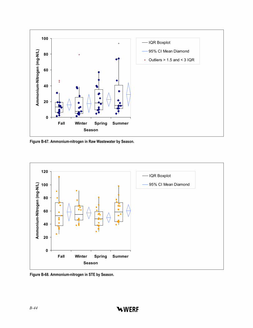
B-44
0
20
40
60
80
100
Fall Winter Spring SummerSeason
Am
mon
ium
-Nitr
ogen
(mg-
N/L
)IQR Boxplot
95% CI Mean Diamond
Outliers > 1.5 and < 3 IQR
Figure B-67. Ammonium-nitrogen in Raw Wastewater by Season.
0
20
40
60
80
100
120
Fall Winter Spring SummerSeason
Am
mon
ium
-Nitr
ogen
(mg-
N/L
)
IQR Boxplot
95% CI Mean Diamond
Figure B-68. Ammonium-nitrogen in STE by Season.
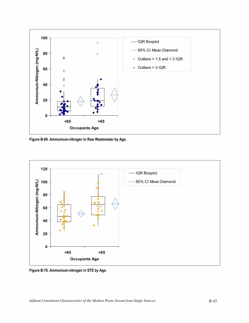
Influent Constituent Characteristics of the Modern Waste Stream from Single Sources
B-45
0
20
40
60
80
100
<65 >65Occupants Age
Am
mon
ium
-Nitr
ogen
(mg-
N/L
)IQR Boxplot
95% CI Mean Diamond
Outliers > 1.5 and < 3 IQR
Outliers > 3 IQR
Figure B-69. Ammonium-nitrogen in Raw Wastewater by Age.
0
20
40
60
80
100
120
<65 >65Occupants Age
Am
mon
ium
-Nitr
ogen
(mg-
N/L
)
IQR Boxplot
95% CI Mean Diamond
Figure B-70. Ammonium-nitrogen in STE by Age.
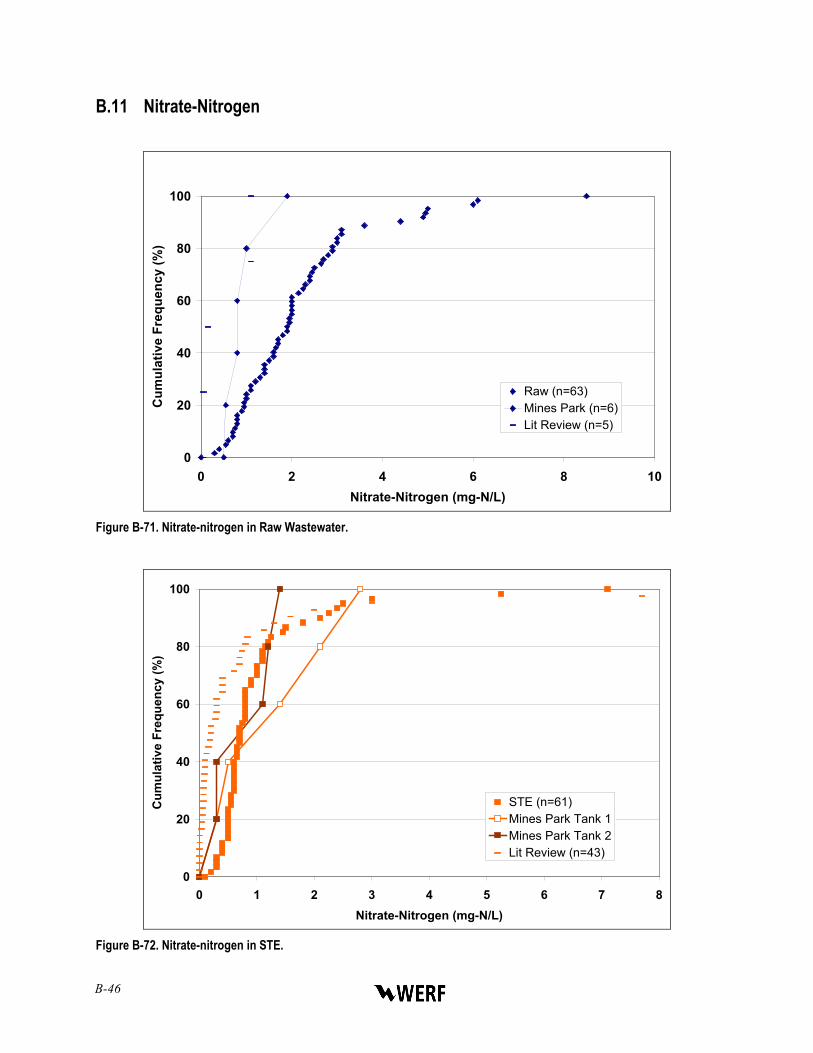
B-46
B.11 Nitrate-Nitrogen
0
20
40
60
80
100
0 2 4 6 8 10Nitrate-Nitrogen (mg-N/L)
Cum
ulat
ive
Freq
uenc
y (%
)
Raw (n=63)Mines Park (n=6)Lit Review (n=5)
Figure B-71. Nitrate-nitrogen in Raw Wastewater.
0
20
40
60
80
100
0 1 2 3 4 5 6 7 8Nitrate-Nitrogen (mg-N/L)
Cum
ulat
ive
Freq
uenc
y (%
)
STE (n=61)Mines Park Tank 1Mines Park Tank 2Lit Review (n=43)
Figure B-72. Nitrate-nitrogen in STE.
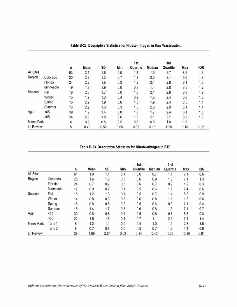
Influent Constituent Characteristics of the Modern Waste Stream from Single Sources
B-47
Table B-22. Descriptive Statistics for Nitrate-nitrogen in Raw Wastewater.
n Mean SD Min 1st
Quartile Median 3rd
Quartile Max IQR All Sites 63 2.1 1.6 0.0 1.1 1.9 2.7 8.5 1.6 Region Colorado 20 2.3 1.3 0.7 1.3 2.0 3.1 5.0 1.8 Florida 24 2.2 1.5 0.3 1.2 2.1 2.8 6.1 1.6 Minnesota 19 1.9 1.9 0.0 0.8 1.4 2.0 8.5 1.2 Season Fall 16 2.3 1.7 0.0 1.0 2.1 2.9 6.0 1.9 Winter 15 1.9 1.3 0.4 0.9 1.5 2.4 5.0 1.5 Spring 16 2.2 1.9 0.6 1.3 1.9 2.4 8.5 1.1 Summer 16 2.2 1.3 0.3 1.5 2.0 2.9 6.1 1.4 Age <65 39 1.9 1.4 0.0 1.0 1.7 2.4 6.1 1.5 >65 24 2.5 1.8 0.6 1.3 2.1 3.1 8.5 1.8 Mines Park 6 0.9 0.5 0.5 0.6 0.8 1.0 1.9 Lit Review 5 0.49 0.56 0.05 0.05 0.16 1.10 1.10 1.05
Table B-23. Descriptive Statistics for Nitrate-nitrogen in STE.
n Mean SD Min 1st
Quartile Median 3rd
Quartile Max IQR All Sites 61 1.0 1.1 0.1 0.6 0.7 1.1 7.1 0.6 Region Colorado 20 1.6 1.8 0.3 0.6 0.9 1.8 7.1 1.3 Florida 24 0.7 0.2 0.3 0.6 0.7 0.9 1.2 0.3 Minnesota 17 0.9 0.7 0.1 0.5 0.6 1.1 2.4 0.6 Season Fall 15 1.2 1.3 0.1 0.5 0.7 1.4 5.3 0.9 Winter 14 0.8 0.3 0.3 0.6 0.8 1.1 1.3 0.6 Spring 16 0.8 0.5 0.2 0.5 0.6 0.9 2.1 0.4 Summer 16 1.4 1.7 0.3 0.6 0.8 1.3 7.1 0.7 Age <65 39 0.8 0.8 0.1 0.5 0.6 0.8 5.3 0.3 >65 22 1.5 1.5 0.4 0.7 1.1 2.1 7.1 1.4 Mines Park Tank 1 6 1.2 1.1 0.0 0.4 1.0 1.9 2.8 1.5 Tank 2 6 0.7 0.6 0.0 0.3 0.7 1.2 1.4 0.9 Lit Review 38 1.09 2.04 0.03 0.14 0.40 1.05 10.30 0.91

B-48
0
2
4
6
8
10
Colorado Florida Minnesota
Region
Nitr
ate-
Nitr
ogen
(mg-
N/L
)IQR Boxplot
95% CI Mean Diamond
Outliers > 1.5 and < 3 IQR
Outliers > 3 IQR
Figure B-73. Nitrate-nitrogen in Raw Wastewater by Region.
0
2
4
6
8
10
Colorado Florida Minnesota
Region
Nitr
ate-
Nitr
ogen
(mg-
N/L
)
IQR Boxplot
95% CI Mean Diamond
Outliers > 1.5 and < 3 IQR
Outliers > 3 IQR
Figure B-74. Nitrate-nitrogen in STE by Region.
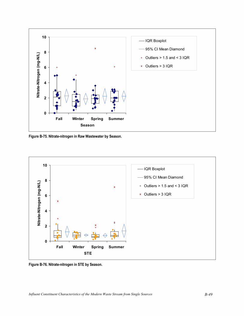
Influent Constituent Characteristics of the Modern Waste Stream from Single Sources
B-49
0
2
4
6
8
10
Fall Winter Spring SummerSeason
Nitr
ate-
Nitr
ogen
(mg-
N/L
)IQR Boxplot
95% CI Mean Diamond
Outliers > 1.5 and < 3 IQR
Outliers > 3 IQR
Figure B-75. Nitrate-nitrogen in Raw Wastewater by Season.
0
2
4
6
8
10
Fall Winter Spring SummerSTE
Nitr
ate-
Nitr
ogen
(mg-
N/L
)
IQR Boxplot
95% CI Mean Diamond
Outliers > 1.5 and < 3 IQR
Outliers > 3 IQR
Figure B-76. Nitrate-nitrogen in STE by Season.
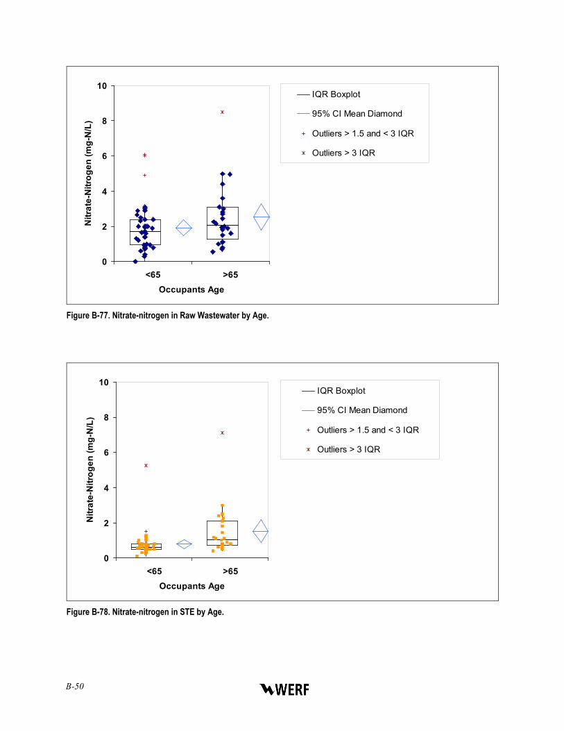
B-50
0
2
4
6
8
10
<65 >65Occupants Age
Nitr
ate-
Nitr
ogen
(mg-
N/L
)IQR Boxplot
95% CI Mean Diamond
Outliers > 1.5 and < 3 IQR
Outliers > 3 IQR
Figure B-77. Nitrate-nitrogen in Raw Wastewater by Age.
0
2
4
6
8
10
<65 >65Occupants Age
Nitr
ate-
Nitr
ogen
(mg-
N/L
)
IQR Boxplot
95% CI Mean Diamond
Outliers > 1.5 and < 3 IQR
Outliers > 3 IQR
Figure B-78. Nitrate-nitrogen in STE by Age.
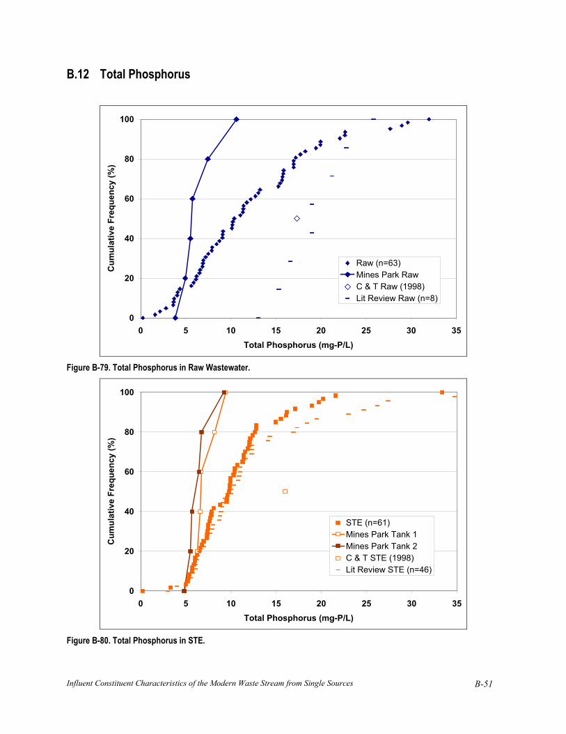
Influent Constituent Characteristics of the Modern Waste Stream from Single Sources
B-51
B.12 Total Phosphorus
0
20
40
60
80
100
0 5 10 15 20 25 30 35Total Phosphorus (mg-P/L)
Cum
ulat
ive
Freq
uenc
y (%
)
Raw (n=63)Mines Park RawC & T Raw (1998)Lit Review Raw (n=8)
Figure B-79. Total Phosphorus in Raw Wastewater.
0
20
40
60
80
100
0 5 10 15 20 25 30 35Total Phosphorus (mg-P/L)
Cum
ulat
ive
Freq
uenc
y (%
)
STE (n=61)Mines Park Tank 1Mines Park Tank 2C & T STE (1998)Lit Review STE (n=46)
Figure B-80. Total Phosphorus in STE.
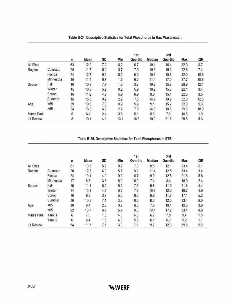
B-52
Table B-24. Descriptive Statistics for Total Phosphorus in Raw Wastewater.
n Mean SD Min 1st
Quartile Median 3rd
Quartile Max IQR All Sites 63 12.0 7.2 0.2 6.7 10.4 16.4 32.0 9.7 Region Colorado 20 11.7 5.2 3.7 7.9 10.3 15.3 22.6 7.4 Florida 24 12.7 9.1 0.2 5.0 10.6 15.8 32.0 10.8 Minnesota 19 11.4 6.7 1.6 6.2 11.4 17.0 27.7 10.8 Season Fall 16 10.8 7.7 1.6 3.7 10.2 15.8 28.9 12.1 Winter 15 10.5 5.9 0.2 5.9 10.2 15.3 22.1 9.4 Spring 16 11.2 4.9 5.9 6.9 9.6 15.4 22.6 8.5 Summer 16 15.3 9.2 2.2 7.5 14.7 19.9 32.0 12.5 Age <65 39 10.8 7.3 0.2 5.9 9.1 15.2 32.0 9.3 >65 24 13.9 6.9 2.2 7.9 14.3 18.8 29.6 10.9 Mines Park 6 6.4 2.4 3.8 5.1 5.6 7.0 10.6 1.9 Lit Review 8 19.1 4.1 13.1 16.3 19.0 21.6 25.8 5.3
Table B-25. Descriptive Statistics for Total Phosphorus in STE.
n Mean SD Min 1st
Quartile Median 3rd
Quartile Max IQR All Sites 61 10.3 5.2 0.2 7.0 9.8 12.1 33.4 5.1 Region Colorado 20 12.3 6.0 5.7 9.1 11.4 12.5 33.4 3.4 Florida 24 10.1 4.9 0.2 6.7 9.9 12.5 21.6 5.8 Minnesota 17 8.3 3.8 5.0 6.0 7.4 8.4 18.9 2.4 Season Fall 15 11.1 5.2 5.2 7.5 9.8 11.9 21.6 4.4 Winter 14 10.1 4.6 0.2 7.3 10.3 12.2 19.7 4.9 Spring 16 9.6 3.7 5.0 6.5 9.9 11.7 17.1 5.2 Summer 16 10.5 7.1 3.3 6.5 8.0 12.5 33.4 6.0 Age <65 39 8.4 2.8 0.2 6.8 7.8 10.4 12.8 3.6 >65 22 13.7 6.7 5.7 9.3 12.4 17.2 33.4 8.0 Mines Park Tank 1 6 7.0 1.6 4.8 6.3 6.7 7.8 9.4 1.5 Tank 2 6 6.4 1.5 4.8 5.6 6.1 6.7 9.2 1.1 Lit Review 54 11.7 7.5 3.0 7.1 9.7 12.3 39.5 5.2
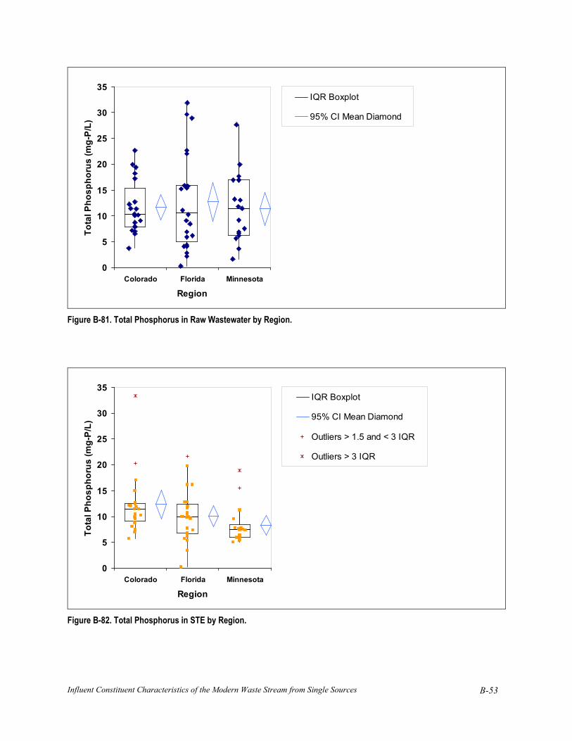
Influent Constituent Characteristics of the Modern Waste Stream from Single Sources
B-53
0
5
10
15
20
25
30
35
Colorado Florida Minnesota
Region
Tota
l Pho
spho
rus
(mg-
P/L)
IQR Boxplot
95% CI Mean Diamond
Figure B-81. Total Phosphorus in Raw Wastewater by Region.
0
5
10
15
20
25
30
35
Colorado Florida Minnesota
Region
Tota
l Pho
spho
rus
(mg-
P/L)
IQR Boxplot
95% CI Mean Diamond
Outliers > 1.5 and < 3 IQR
Outliers > 3 IQR
Figure B-82. Total Phosphorus in STE by Region.
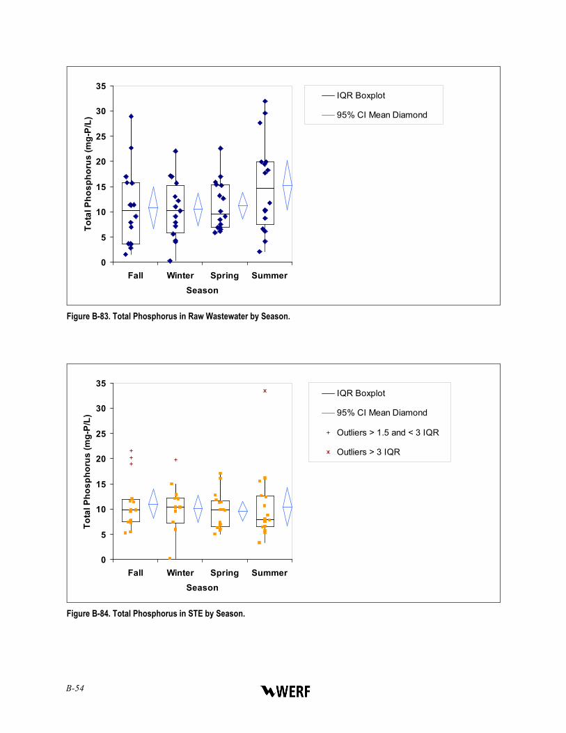
B-54
0
5
10
15
20
25
30
35
Fall Winter Spring SummerSeason
Tota
l Pho
spho
rus
(mg-
P/L)
IQR Boxplot
95% CI Mean Diamond
Figure B-83. Total Phosphorus in Raw Wastewater by Season.
0
5
10
15
20
25
30
35
Fall Winter Spring SummerSeason
Tota
l Pho
spho
rus
(mg-
P/L)
IQR Boxplot
95% CI Mean Diamond
Outliers > 1.5 and < 3 IQR
Outliers > 3 IQR
Figure B-84. Total Phosphorus in STE by Season.

Influent Constituent Characteristics of the Modern Waste Stream from Single Sources
B-55
0
5
10
15
20
25
30
35
<65 >65Occupants Age
Tota
l Pho
spho
rus
(mg-
P/L)
IQR Boxplot
95% CI Mean Diamond
Outliers > 1.5 and < 3 IQR
Figure B-85. Total Phosphorus in Raw Wastewater by Age.
0
5
10
15
20
25
30
35
<65 >65Occupants Age
Tota
l Pho
spho
rus
(mg-
P/L)
IQR Boxplot
95% CI Mean Diamond
Outliers > 1.5 and < 3 IQR
Figure B-86. Total Phosphorus in STE by Age.

B-56
Influent Constituent Characteristics of the Modern Waste Stream from Single Sources
C-1
APPENDIX C
TIER 2: OIL AND GREASE AND MICROORGANISMS
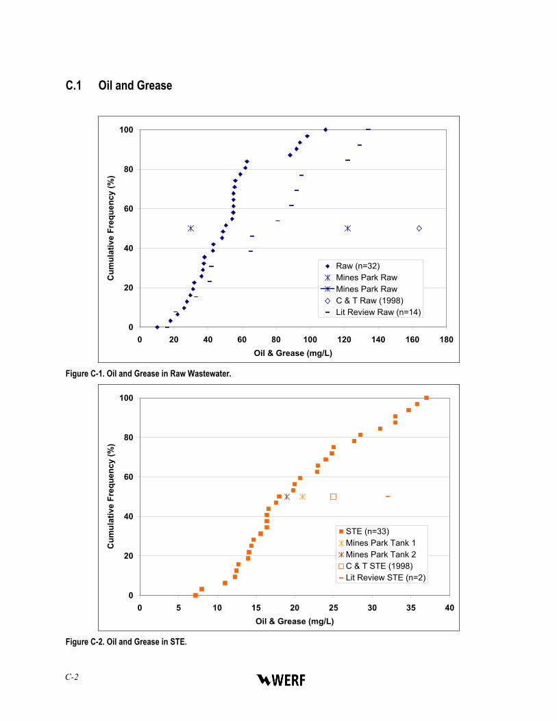
C-2
C.1 Oil and Grease
0
20
40
60
80
100
0 20 40 60 80 100 120 140 160 180Oil & Grease (mg/L)
Cum
ulat
ive
Freq
uenc
y (%
)
Raw (n=32)Mines Park RawMines Park RawC & T Raw (1998)Lit Review Raw (n=14)
Figure C-1. Oil and Grease in Raw Wastewater.
0
20
40
60
80
100
0 5 10 15 20 25 30 35 40Oil & Grease (mg/L)
Cum
ulat
ive
Freq
uenc
y (%
)
STE (n=33)Mines Park Tank 1Mines Park Tank 2C & T STE (1998)Lit Review STE (n=2)
Figure C-2. Oil and Grease in STE.

Influent Constituent Characteristics of the Modern Waste Stream from Single Sources
C-3
Table C-1. Descriptive Statistics for Oil and Grease in Raw Wastewater.
n Mean SD Min 1st
Quartile Median 3rd
Quartile Max IQR All Sites 32 51 24 10 35 50 57 109 22 Region Colorado 9 54 26 18 37 55 62 94 54 Florida 17 55 25 10 43 54 59 109 55 Minnesota 6 35 13 22 26 29 44 55 35 Age <65 21 46 25 10 30 38 55 109 25 >65 11 60 19 37 52 56 61 98 9 Mines Park 2 30 122 Lit Review 14 73 39 16 41 74 94 134 53
Table C-2. Descriptive Statistics for Oil and Grease in STE.
n Mean SD Min 1st
Quartile Median 3rd
Quartile Max IQR All Sites 33 21 8 7 14 18 25 37 11 Region Colorado 11 24 9 8 19 24 32 37 24 Florida 17 20 8 7 14 17 25 36 20 Minnesota 5 16 5 11 13 15 16 23 16 Age <65 22 20 8 7 14 18 25 36 11 >65 11 20 9 8 15 16 26 37 10 Mines Park Tank 1 2 20 21 Tank 2 2 17 21 Lit Review 2 31 32

C-4
0
20
40
60
80
100
120
Colorado Florida Minnesota
Region
Oil
& G
reas
e (m
g/L)
IQR Boxplot
95% CI Mean Diamond
Outliers > 1.5 and < 3 IQR
Figure C-3. Oil and Grease in Raw Wastewater by Region.
0
10
20
30
40
50
Colorado Florida Minnesota
Region
Oil
& G
reas
e (m
g/L)
IQR Boxplot
95% CI Mean Diamond
Figure C-4. Oil and Grease in STE by Region.
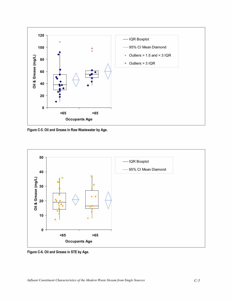
Influent Constituent Characteristics of the Modern Waste Stream from Single Sources
C-5
0
20
40
60
80
100
120
<65 >65Occupants Age
Oil
& G
reas
e (m
g/L)
IQR Boxplot
95% CI Mean Diamond
Outliers > 1.5 and < 3 IQR
Outliers > 3 IQR
Figure C-5. Oil and Grease in Raw Wastewater by Age.
0
10
20
30
40
50
<65 >65Occupants Age
Oil
& G
reas
e (m
g/L)
IQR Boxplot
95% CI Mean Diamond
Figure C-6. Oil and Grease in STE by Age.

C-6
C.2 Fecal Coliforms
0
20
40
60
80
100
1.E+03 1.E+04 1.E+05 1.E+06 1.E+07 1.E+08 1.E+09Fecal Coliforms (cfu/100 mL)
Cum
ulat
ive
Freq
uenc
y (%
)
Raw (n=59)Lit Review (n=5)
Figure C-7. Fecal Coliforms in Raw Wastewater.
0
20
40
60
80
100
1.E+03 1.E+04 1.E+05 1.E+06 1.E+07 1.E+08 1.E+09Fecal Coliforms (MPN/100 mL)
Cum
ulat
ive
Freq
uenc
y (%
)
STE (n=56)Lit Review (n=62)
Figure C-8. Fecal Coliforms in STE.
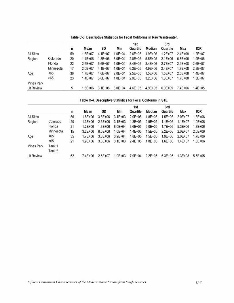
Influent Constituent Characteristics of the Modern Waste Stream from Single Sources
C-7
Table C-3. Descriptive Statistics for Fecal Coliforms in Raw Wastewater.
n Mean SD Min 1st
Quartile Median 3rd
Quartile Max IQR All Sites 59 1.6E+07 4.1E+07 1.0E+04 2.6E+05 1.9E+06 1.2E+07 2.4E+08 1.2E+07 Region Colorado 20 1.4E+06 1.8E+06 3.0E+04 2.0E+05 5.5E+05 2.1E+06 6.8E+06 1.9E+06 Florida 22 2.5E+07 5.6E+07 1.0E+04 8.4E+05 3.4E+06 2.7E+07 2.4E+08 2.6E+07 Minnesota 17 2.0E+07 4.1E+07 1.0E+04 6.3E+05 4.9E+06 2.4E+07 1.7E+08 2.3E+07 Age <65 36 1.7E+07 4.6E+07 2.0E+04 2.5E+05 1.5E+06 1.5E+07 2.5E+08 1.4E+07 >65 23 1.4E+07 3.6E+07 1.0E+04 2.9E+05 3.2E+06 1.3E+07 1.7E+08 1.3E+07 Mines Park Lit Review 5 1.8E+06 3.1E+06 3.0E+04 4.6E+05 4.9E+05 6.0E+05 7.4E+06 1.4E+05
Table C-4. Descriptive Statistics for Fecal Coliforms in STE.
n Mean SD Min 1st
Quartile Median 3rd
Quartile Max IQR All Sites 56 1.8E+06 3.6E+06 3.1E+03 2.0E+05 4.8E+05 1.5E+06 2.0E+07 1.3E+06 Region Colorado 20 1.3E+06 2.6E+06 3.1E+03 1.3E+05 2.9E+05 1.1E+06 1.1E+07 1.0E+06 Florida 21 1.2E+06 1.3E+06 8.0E+04 3.6E+05 9.0E+05 1.7E+06 5.3E+06 1.3E+06 Minnesota 15 3.2E+06 6.0E+06 1.0E+04 1.4E+05 4.5E+05 2.2E+06 2.0E+07 2.0E+06 Age <65 35 1.7E+06 3.6E+06 3.9E+04 1.8E+05 4.5E+05 1.9E+06 2.0E+07 1.7E+06 >65 21 1.9E+06 3.6E+06 3.1E+03 2.4E+05 4.8E+05 1.6E+06 1.4E+07 1.3E+06 Mines Park Tank 1 Tank 2 Lit Review 62 7.4E+06 2.6E+07 1.9E+03 7.9E+04 2.2E+05 6.3E+05 1.3E+08 5.5E+05
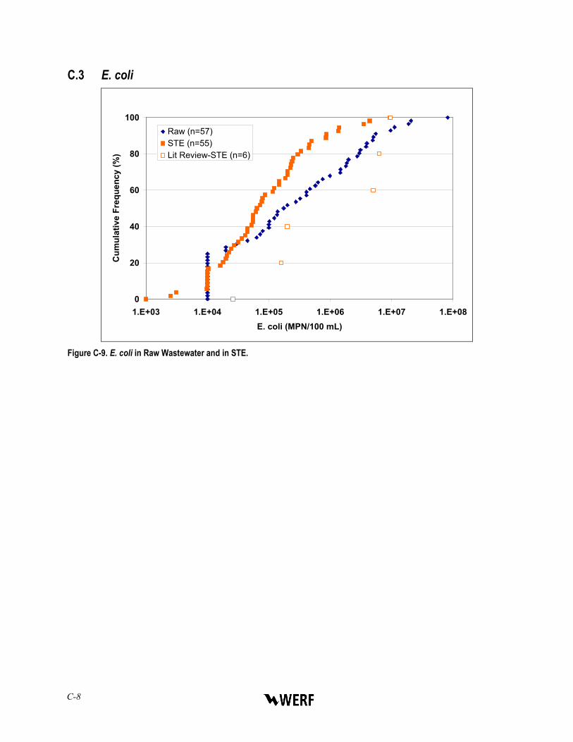
C-8
C.3 E. coli
0
20
40
60
80
100
1.E+03 1.E+04 1.E+05 1.E+06 1.E+07 1.E+08E. coli (MPN/100 mL)
Cum
ulat
ive
Freq
uenc
y (%
)
Raw (n=57)STE (n=55)Lit Review-STE (n=6)
Figure C-9. E. coli in Raw Wastewater and in STE.

Influent Constituent Characteristics of the Modern Waste Stream from Single Sources
C-9
Table C-5. Descriptive Statistics for E. coli in Raw Wastewater.
n Mean SD Min 1st
Quartile Median 3rd
Quartile Max IQR All Sites 57 3.3E+06 1.1E+07 1.0E+04 1.0E+04 1.8E+05 1.9E+06 8.2E+07 1.9E+06 Region Colorado 18 1.4E+05 4.6E+05 1.0E+04 1.0E+04 1.0E+04 6.4E+04 2.0E+06 5.4E+04 Florida 22 5.7E+06 1.8E+07 1.0E+04 1.0E+05 4.1E+05 3.0E+06 8.2E+07 2.9E+06 Minnesota 17 3.6E+06 5.2E+06 1.0E+04 1.7E+05 1.5E+06 5.2E+06 1.9E+07 5.0E+06 Age <65 35 1.7E+06 3.9E+06 1.0E+04 2.0E+04 1.4E+05 1.7E+06 2.1E+07 1.7E+06 >65 22 5.9E+06 1.7E+07 1.0E+04 1.0E+04 3.1E+05 3.3E+06 8.2E+07 3.2E+06 Mines Park Lit Review nd
Table C-6. Descriptive Statistics for E. coli in STE.
n Mean SD Min 1st
Quartile Median 3rd
Quartile Max IQR All Sites 55 4.9E+05 1.4E+06 1.0E+03 2.2E+04 6.4E+04 2.3E+05 9.4E+06 2.1E+05 Region Colorado 19 7.1E+04 1.2E+05 1.0E+03 1.0E+04 2.0E+04 6.1E+04 4.6E+05 5.1E+04 Florida 21 2.2E+05 3.3E+05 1.0E+04 4.5E+04 7.9E+04 2.3E+05 1.4E+06 1.9E+05 Minnesota 15 1.4E+06 2.6E+06 9.8E+03 8.0E+04 2.3E+05 1.3E+06 9.4E+06 1.2E+06 Age <65 34 3.6E+05 9.4E+05 9.8E+03 2.0E+04 6.0E+04 2.0E+05 4.4E+06 1.8E+05 >65 21 6.9E+05 2.0E+06 1.0E+03 2.2E+04 1.2E+05 4.5E+05 9.4E+06 4.3E+05 Mines Park Tank 1 Tank 2 Lit Review 6 3.5E+06 4.0E+06 2.6E+04 1.7E+05 2.6E+06 6.0E+06 9.5E+06 5.8E+06

C-10

Influent Constituent Characteristics of the Modern Waste Stream from Single Sources D-1
APPENDIX D
WEEKLY AND DAILY VARIATIONS

D-2
Table D-1. Specific Water Use during the Course of the Week at Site C-5.
Activity Monday Tuesday Wednesday Thursday Friday Saturday Sunday Showers 2 2 1 Baths Toilet Flushes 15 20 22 16 20 16 18 Toilet Cleaning Hand Washes 14 22 24 18 23 19 21 Sink Cleaning Teeth Brushing 1 2 4 2 3 1 3 Dishwashing (machine) 1 1 1 Dishwashing (in sink) 1 1 Laundry (machine) 1 1 1 1 Laundry (in sink) Miscellaneous sink use Other
Table D-2. Specific Water Use during the Course of the Week at Site F-2.
Activity Monday Tuesday Wednesday Thursday Friday Saturday Sunday Showers 2 2 1 2 5 Baths 1 Toilet Flushes 3 8 5 9 13 11 10 Toilet Cleaning 2 Hand Washes 4 12 5 9 12 9 6 Sink Cleaning 1 Teeth Brushing 4 4 4 4 4 4 4 Dishwashing (machine) 1 1 Dishwashing (in sink) 1 1 Laundry (machine) 2 2 1 1 Laundry (in sink) Miscellaneous sink use Other (tub cleaning) 1
Table D-3. Specific Water Use during the Course of the Week at Site M-2.
Activity Monday Tuesday Wednesday Thursday Friday Saturday Sunday Showers 1 1 1 1 1 3 Baths 1 1 1 Toilet Flushes 8 7 8 5 7 8 5 Toilet Cleaning Hand Washes 9 10 12 5 8 5 4 Sink Cleaning 1 3 Teeth Brushing 3 3 3 3 3 3 3 Dishwashing (machine) 2 1 1 2 1 Dishwashing (in sink) 2 3 5 3 1 4 Laundry (machine) 2 2 3 1 2 Laundry (in sink) 1 Miscellaneous sink use Other
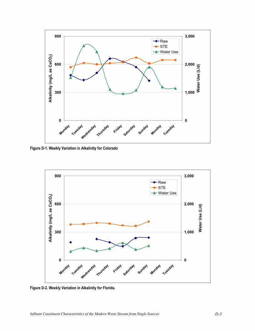
Influent Constituent Characteristics of the Modern Waste Stream from Single Sources D-3
0
300
600
900
Monday
Tuesday
Wednes
day
Thursday
Friday
Saturd
ay
Sunday
Monday
Tuesday
Alk
alin
ity (m
g/L
as C
aCO
3)
0
1,000
2,000
3,000
Wat
er U
se (L
/d)
RawSTEWater Use
Figure D-1. Weekly Variation in Alkalinity for Colorado
0
300
600
900
Monday
Tuesday
Wednes
day
Thursday
Friday
Saturd
ay
Sunday
Monday
Tuesday
Alk
alin
ity (m
g/L
as C
aCO
3)
0
1,000
2,000
3,000
Wat
er U
se (L
/d)
RawSTEWater Use
Figure D-2. Weekly Variation in Alkalinity for Florida.
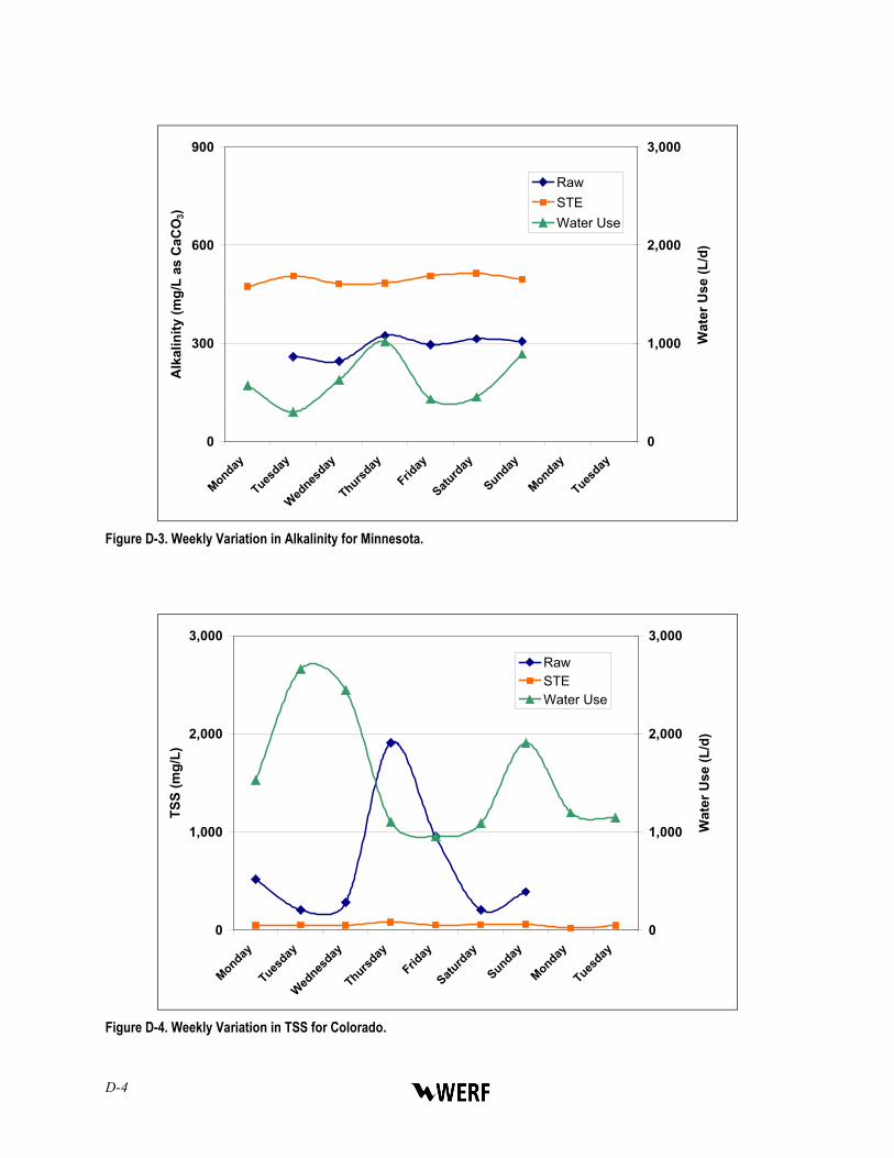
D-4
0
300
600
900
Monday
Tuesday
Wednes
day
Thursday
Friday
Saturd
ay
Sunday
Monday
Tuesday
Alk
alin
ity (m
g/L
as C
aCO
3)
0
1,000
2,000
3,000
Wat
er U
se (L
/d)
RawSTEWater Use
Figure D-3. Weekly Variation in Alkalinity for Minnesota.
0
1,000
2,000
3,000
Monday
Tuesday
Wednes
day
Thursday
Friday
Saturd
ay
Sunday
Monday
Tuesday
TSS
(mg/
L)
0
1,000
2,000
3,000
Wat
er U
se (L
/d)
RawSTEWater Use
Figure D-4. Weekly Variation in TSS for Colorado.

Influent Constituent Characteristics of the Modern Waste Stream from Single Sources D-5
0
1,000
2,000
3,000
Monday
Tuesday
Wednes
day
Thursday
Friday
Saturd
ay
Sunday
Monday
Tuesday
TSS
(mg/
L)
0
1,000
2,000
3,000
Wat
er U
se (L
/d)
RawSTEWater Use
Figure D-5. Weekly Variation in TSS for Site Florida.
0
1,000
2,000
3,000
Monday
Tuesday
Wednes
day
Thursday
Friday
Saturd
ay
Sunday
Monday
Tuesday
TSS
(mg/
L)
0
1,000
2,000
3,000
Wat
er U
se (L
/d)
RawSTEWater Use
Figure D-6. Weekly Variation in TSS for Minnesota.
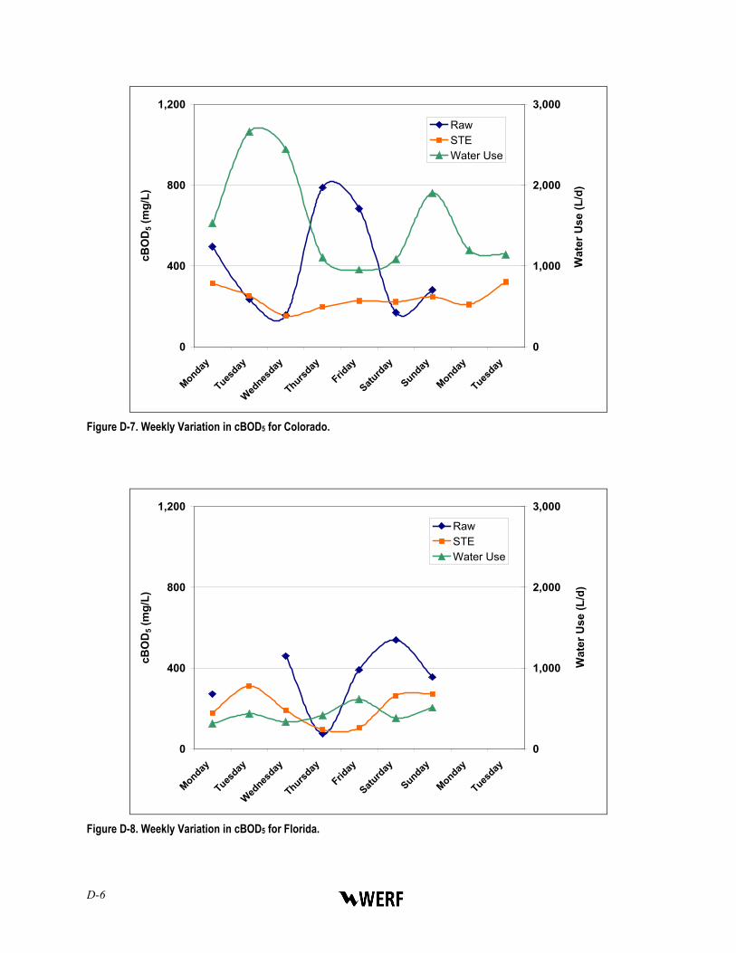
D-6
0
400
800
1,200
Monday
Tuesday
Wednes
day
Thursday
Friday
Saturd
ay
Sunday
Monday
Tuesday
cBO
D5 (
mg/
L)
0
1,000
2,000
3,000
Wat
er U
se (L
/d)
RawSTEWater Use
Figure D-7. Weekly Variation in cBOD5 for Colorado.
0
400
800
1,200
Monday
Tuesday
Wednes
day
Thursday
Friday
Saturd
ay
Sunday
Monday
Tuesday
cBO
D5 (
mg/
L)
0
1,000
2,000
3,000
Wat
er U
se (L
/d)
RawSTEWater Use
Figure D-8. Weekly Variation in cBOD5 for Florida.

Influent Constituent Characteristics of the Modern Waste Stream from Single Sources D-7
0
300
600
900
1,200
Monday
Tuesday
Wednes
day
Thursday
Friday
Saturd
ay
Sunday
Monday
Tuesday
cBO
D5 (
mg/
L)
0
1,000
2,000
3,000
Wat
er U
se (L
/d)
RawSTEWater Use
Figure D-9. Weekly Variation in cBOD5 for Minnesota.
0
100
200
300
Monday
Tuesday
Wednes
day
Thursday
Friday
Saturd
ay
Sunday
Monday
Tuesday
Tota
l Nitr
ogen
(mg-
N/L
)
0
1,000
2,000
3,000
Wat
er U
se (L
/d)
RawSTEWater Use
Figure D-10. Weekly Variation in Total Nitrogen for Colorado.
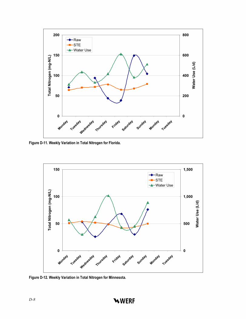
D-8
0
50
100
150
200
Monday
Tuesday
Wednes
day
Thursday
Friday
Saturd
ay
Sunday
Monday
Tuesday
Tota
l Nitr
ogen
(mg-
N/L
)
0
200
400
600
800
Wat
er U
se (L
/d)
RawSTEWater Use
Figure D-11. Weekly Variation in Total Nitrogen for Florida.
0
50
100
150
Monday
Tuesday
Wednes
day
Thursday
Friday
Saturd
ay
Sunday
Monday
Tuesday
Tota
l Nitr
ogen
(mg-
N/L
)
0
500
1,000
1,500
Wat
er U
se (L
/d)
RawSTEWater Use
Figure D-12. Weekly Variation in Total Nitrogen for Minnesota.
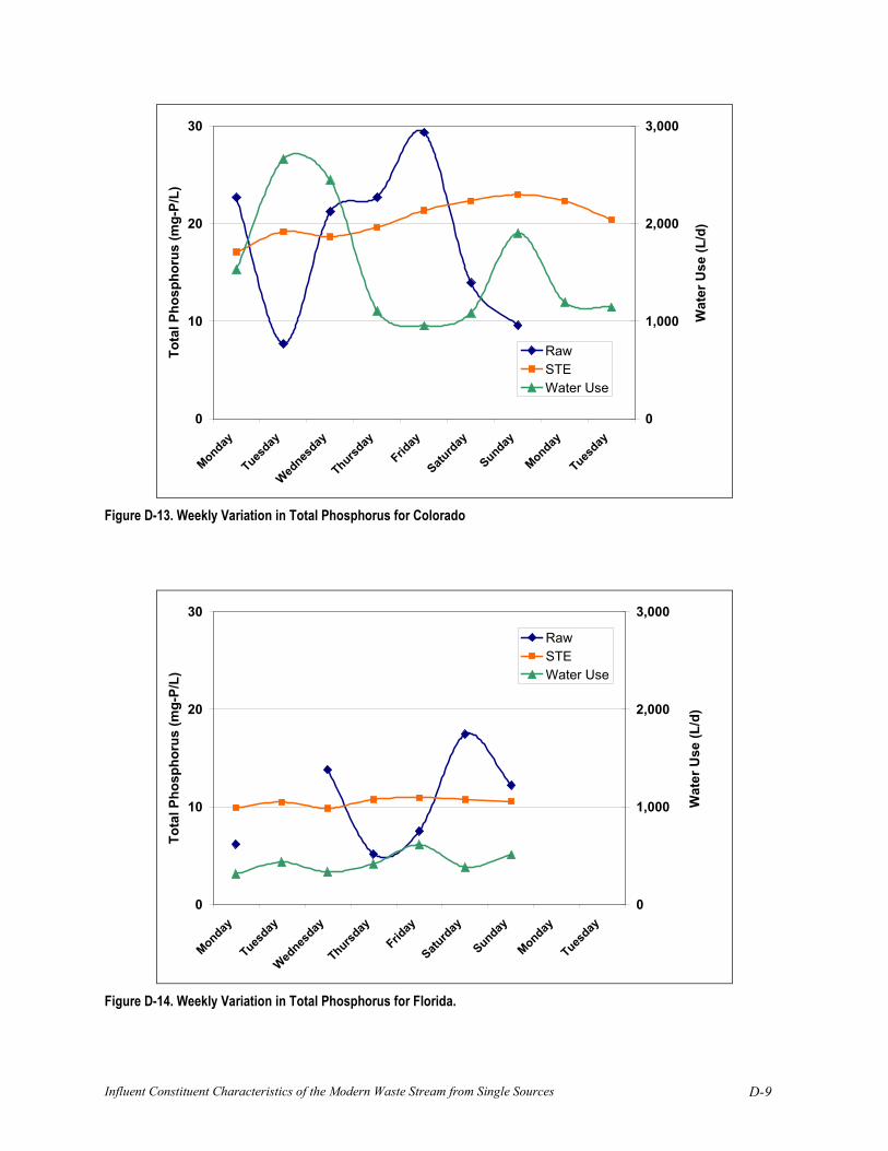
Influent Constituent Characteristics of the Modern Waste Stream from Single Sources D-9
0
10
20
30
Monday
Tuesday
Wednes
day
Thursday
Friday
Saturd
ay
Sunday
Monday
Tuesday
Tota
l Pho
spho
rus
(mg-
P/L)
0
1,000
2,000
3,000
Wat
er U
se (L
/d)
RawSTEWater Use
Figure D-13. Weekly Variation in Total Phosphorus for Colorado
0
10
20
30
Monday
Tuesday
Wednes
day
Thursday
Friday
Saturd
ay
Sunday
Monday
Tuesday
Tota
l Pho
spho
rus
(mg-
P/L)
0
1,000
2,000
3,000
Wat
er U
se (L
/d)
RawSTEWater Use
Figure D-14. Weekly Variation in Total Phosphorus for Florida.
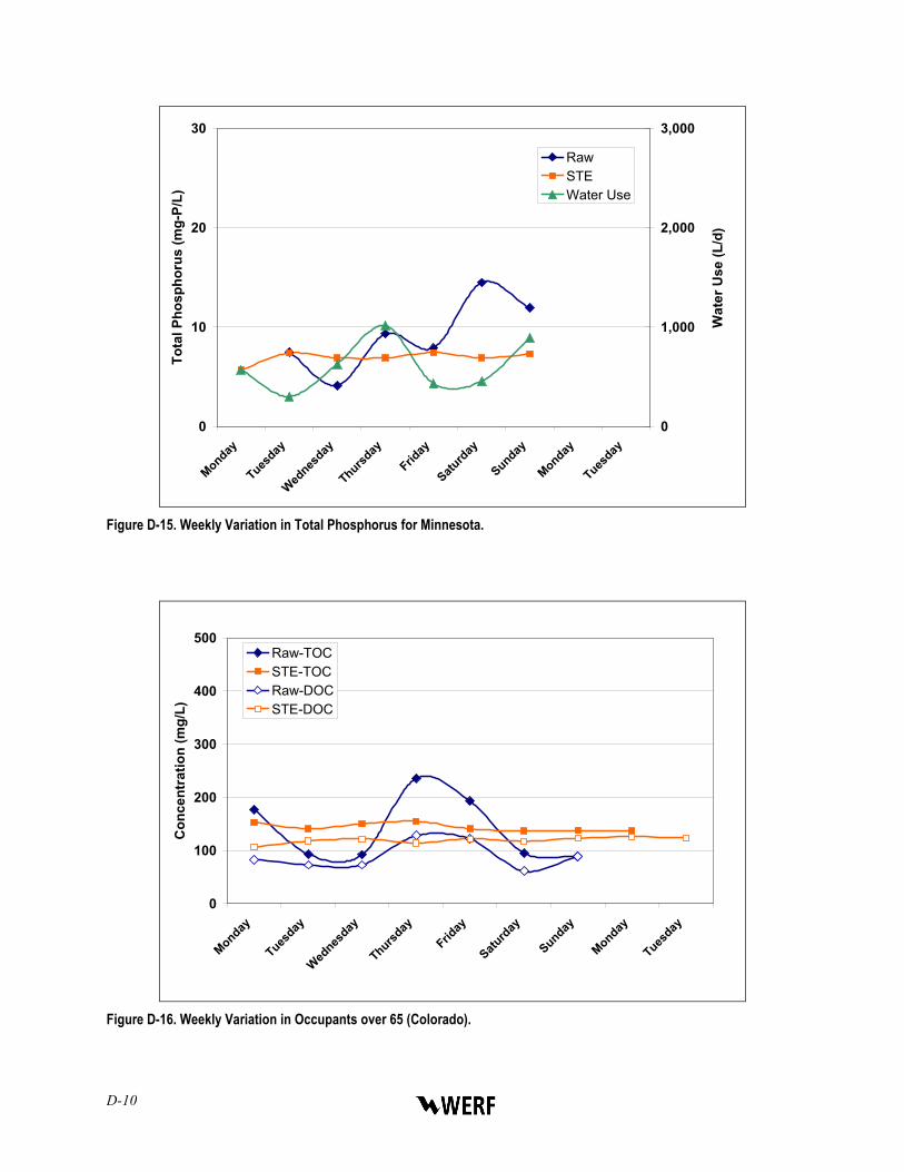
D-10
0
10
20
30
Monday
Tuesday
Wednes
day
Thursday
Friday
Saturd
ay
Sunday
Monday
Tuesday
Tota
l Pho
spho
rus
(mg-
P/L)
0
1,000
2,000
3,000
Wat
er U
se (L
/d)
RawSTEWater Use
Figure D-15. Weekly Variation in Total Phosphorus for Minnesota.
0
100
200
300
400
500
Monday
Tuesday
Wednes
day
Thursday
Friday
Saturd
ay
Sunday
Monday
Tuesday
Con
cent
ratio
n (m
g/L)
Raw-TOCSTE-TOCRaw-DOCSTE-DOC
Figure D-16. Weekly Variation in Occupants over 65 (Colorado).
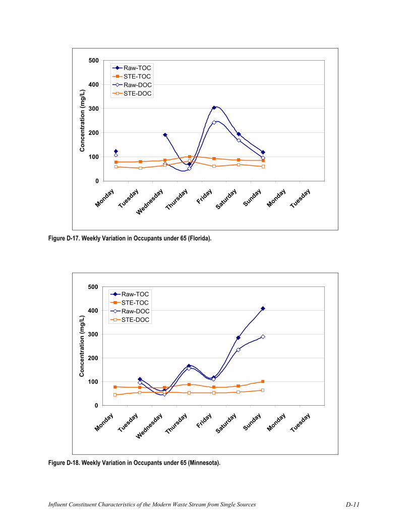
Influent Constituent Characteristics of the Modern Waste Stream from Single Sources D-11
0
100
200
300
400
500
Monday
Tuesday
Wednes
day
Thursday
Friday
Saturd
ay
Sunday
Monday
Tuesday
Con
cent
ratio
n (m
g/L)
Raw-TOCSTE-TOCRaw-DOCSTE-DOC
Figure D-17. Weekly Variation in Occupants under 65 (Florida).
0
100
200
300
400
500
Monday
Tuesday
Wednes
day
Thursday
Friday
Saturd
ay
Sunday
Monday
Tuesday
Con
cent
ratio
n (m
g/L)
Raw-TOCSTE-TOCRaw-DOCSTE-DOC
Figure D-18. Weekly Variation in Occupants under 65 (Minnesota).

D-12
0%
20%
40%
60%
80%
100%
COD cBOD5 TN NH4-N NO3-N TP
Toilet UseMixed UseLaundryDishwasher
Figure D-19. Percent of Constituent Contributed from Various Water Use Activities during Daily Trend Sampling (Colorado, Three Sites).
0%
20%
40%
60%
80%
100%
COD cBOD5 TN NH4-N NO3-N TP
Toilet UseMixed UseLaundryDishwasher
Figure D-20. Percent of Constituent Contributed from Various Water Use Activities during Daily Trend Sampling (Minnesota, Three Sites).
Influent Constituent Characteristics of the Modern Waste Stream from Single Sources R-1
REFERENCES American Housing Survey (AHS) (2006). http://www.census.gov/hhes/www/housing/ahs/ahs.html
Analyse-it, version 1.73 Statistical Software. Analyse-it Software, Ltd.
Ahel, M., T. Conrad, and W. Giger (1987). Persistent organic chemicals in sewage effluents. 3. Determinations of nonylphenoxy carboxylic acids by high-resolution gas chromatography/mass spectrometry and high-performance liquid chromatography. Environmental Science & Technology. 27: 697-703.
American Public Health Association (APHA) (2005). Standard Methods for the Examination of Water and Wastewater. Washington, D.C., American Public Health Association.
Barber, L.B., G.K. Brown, and S.D. Zaugg (2000). Potential endocrine disrupting organic chemicals in treated municipal wastewater and river water. In Analysis of Environmental Endocrine Disruptors. Keith, L.H., T.L. Jones-Lepp, and L.L. Needham, Eds. ACS Symposium Series 747. American Chemical Society: Washington, D.C. pp. 97-123.
Bounds, T.R. (1997). Design and performance of septic tanks. Site Characterization and Design of Onsite Septic Systems ASTM STP 901, M.S. Bedinger, A.I. Johnson, and J.S. Fleming, Eds. American Society for Testing Materials, Philadelphia, PA.
Carrara, C., C.J. Ptacek, W.D. Robertson, D.W. Blowes, M.C. Moncur, E. Sverko, and S. Backus (2008). Fate of pharmaceutical and trace organic compounds in three septic plumes, Ontario, Canada. Environmental Science & Technology. 42: 2805-2811.
Chihara, R.J., M.A. Sullivan, C.A. Likirdopulos, O.D.S. III, C.L. Burch, and M.D. Sobsey (2005). Comparison of methods for detection of fecal coliforms and E. coli in agricultural and municipal wastewater systems. Proceedings of the Animal Waste Management Symposium.
Conn, K.E. (2008). Occurrence and fate of endocrine-disrupting compounds and trace organic contaminants in onsite wastewater treatment systems. Ph.D. Dissertation. Environmental Science & Engineering, Colorado School of Mines, Golden, CO.
Crites, R. and G. Tchobanoglous (1998). Small and Decentralized Wastewater Management Systems. McGraw-Hill, San Francisco, CA.
Edvardsson, C.M. and D.R. Spears (2000). Case study of an advanced on-site treatment system connected to a single-family residence. Proceedings of the National Onsite Wastewater Recycling Association 2000 Conference, Onsite: The future of water quality.
HACH (1998). Water Analysis Handbook. 2nd ed. HACH Chemical Company, Loveland, CO. Kari, F.G. and W. Giger (1996). Speciation and fate of ethylenediaminetetraacetate (EDTA) in municipal wastewater treatment. Water Research. 30: 122-134.
Lowe, K.S., N. Rothe, J. Tomaras, K. DeJong, M. Tucholke, J. Drewes, J. McCray, and J. Munakata-Marr (2007). Influent Constituent Characteristics of the Modern Waste Stream from Single Sources: Literature Review. Water Environment Research Foundation. 04-DEC-1. 89pg. PDF available at: www.ndwrcdp.org/publications.

R-2
Mayer, P.W., W.B. DeOreo, E.M. Optiz, J.C. Kiefer, W.Y. Davis, B. Dziegielewski, and J.O. Nelson (1999). Residential End Uses of Water, American Water Works Association Research Foundation, Denver, CO, 310 p.
McCray, J.E., S.L. Kirkland, R.L. Siegrist, and G.D. Thyne (2005). Model Parameters for Simulating Fate and Transport of On-Site Wastewater Nutrients. Ground Water. 43(4): 628-639.
Metcalf and Eddy, Inc. (1991). Wastewater Engineering: Treatment, Disposal and Reuse. 3rd Ed. McGraw-Hill, New York.
Moore, D.S. and G.P. McCabe (1999). Introduction to the Practice of Statistics. 3rd ed. W.H. Freeman and Company, New York.
Reddersen, K. and T. Heberer. (2003). Multi-compound methods for the detection of pharmaceutical residues in various waters applying solid phase extraction (SPE) and gas chromatography with mass spectrometric (GC-MS) detection. Journal of Separation Science. 26: 1443-1450.
Reynolds, T.D. and P.A. Richards (1996). Unit Operations and Processes in Environmental Engineering. Second ed. PWS Publishing Company.
Selvakumar, A., M. Borst, M. Boner, and P. Mallon (2004). Effects of sample holding time on concentrations of microorganisms in water samples. Water Environment Research. 76(1):67-72.
Shane, S., B. Vanderford, J.E. Drewes, E. Dickenson, E. Snyder, G. Bruce, and R. Pleus (2008). State of Knowledge of EDCs and Pharmaceuticals in Drinking Water. Final Report. AWWA Research Foundation. Denver, CO.
Siegrist, R.L. (2001). Perspectives on the science and engineering of onsite wastewater systems. Small Flows, 2(4): 8-13.
Siegrist, R.L. and W.C. Boyle (1987). Wastewater-induced soil clogging development, Journal of Environmental Engineering, 113(3): 550-556.
Snedecor, G.W. and W.G. Cochran (1980). Statistical Methods, 7th Edition. Iowa State University Press.
Thomas, P.M. and G.D. Foster (2005). Tracking acidic pharmaceuticals, caffeine, and triclosan through the wastewater treatment process. Environmental Toxicology & Chemistry. 24: 25-30.
U.S. EPA (1997). Response to Congress on Use of Decentralized Wastewater Treatment Systems. U.S. Environmental Protection Agency, Office of Water, Washington, D.C.
U.S. EPA (2002). Onsite Wastewater Treatment Systems Manual. Report No. 625/R-00/008. U.S. Environmental Protection Agency, Cincinnati, OH.
Van Cuyk, S. (2003). Fate of Virus During Wastewater Renovation in Soil Porous Media Biofilters. Ph.D. Dissertation. Environmental Science and Engineering Division, Colorado School of Mines. Golden, CO.
Yakub, G.P., D.A. Castric, K.L. Stadterman-Knauer, M.J. Tobin, M. Blazina, T.N. Heineman, G.Y. Yee, and L. Frazier (2002). Evaluation of Colilert and Enterolert defined substrate methodology for wastewater applications. Water Environ Research. 74(2):131-5.
A l a b a m aMontgomery Water Works &
Sanitary Sewer Board
A l a s k aAnchorage Water &
Wastewater Utility
A r i z o n aAvondale, City ofGlendale, City of,
Utilities DepartmentMesa, City ofPeoria, City ofPhoenix Water Services Dept.Pima County Wastewater
ManagementSafford, City ofTempe, City of
A r k a n s a sLittle Rock Wastewater Utility
C a l i f o rn i aCentral Contra Costa
Sanitary DistrictCorona, City ofCrestline Sanitation DistrictDelta Diablo
Sanitation DistrictDublin San Ramon Services
DistrictEast Bay Dischargers
AuthorityEast Bay Municipal
Utility DistrictEl Dorado Irrigation DistrictFairfield-Suisun Sewer DistrictFresno Department of Public
UtilitiesInland Empire Utilities AgencyIrvine Ranch Water DistrictLas Gallinas Valley Sanitary
DistrictLas Virgenes Municipal
Water DistrictLivermore, City ofLos Angeles, City ofLos Angeles County,
Sanitation Districts ofNapa Sanitation DistrictNovato Sanitary DistrictOrange County Sanitation
DistrictPalo Alto, City ofRiverside, City of Sacramento Regional County
Sanitation DistrictSan Diego Metropolitan
Wastewater Depart m e n t ,City of
San Francisco,City & County of
San Jose, City ofSanta Barbara, City ofSanta Cruz, City ofSanta Rosa, City ofSouth Bayside System
Authority
South Coast Water DistrictSouth Orange County
Wastewater AuthorityStege Sanitary DistrictSunnyvale, City ofUnion Sanitary DistrictWest Valley Sanitation District
C o l o r a d oAurora, City ofBoulder, City ofGreeley, City ofLittleton/Englewood Water
Pollution Control PlantMetro Wastewater
Reclamation District, Denver
C o n n e c t i c u tGreater New Haven WPCAStamford, City of
District of ColumbiaDistrict of Columbia Water &
Sewer Authority
F l o r i d aBroward, County ofFort Lauderdale, City ofJacksonville Electric Authority
(JEA)Miami-Dade Water &
Sewer AuthorityOrange County Utilities
DepartmentPinellas, County ofReedy Creek Improvement
D i s t r i c tSeminole County
Environmental ServicesSt. Petersburg, City ofTallahassee, City ofTampa, City ofToho Water AuthorityWest Palm Beach, City ofG e o rg i aAtlanta Department of
Watershed ManagementAugusta, City of Clayton County Water
Authority Cobb County Water SystemColumbus Water WorksFulton County Gwinnett County Department
of Public UtilitiesSavannah, City of
H a w a i iHonolulu, City & County of
I d a h oBoise, City of
I l l i n o i sDecatur, Sanitary District ofGreater Peoria
Sanitary DistrictKankakee River Metropolitan
AgencyMetropolitan Water
Reclamation District ofGreater Chicago
Wheaton Sanitary District
I o w aAmes, City ofCedar Rapids Wa s t e w a t e r
F a c i l i t yDes Moines, City ofIowa City
K a n s a sJohnson County WastewaterLenexa, City ofUnified Government of
Wyandotte County/Kansas City, City of
K e n t u c k yLouisville & Jefferson County
Metropolitan Sewer District
L o u i s i a n aSewerage & Water Board
of New Orleans
M a i n eBangor, City ofPortland Water District
M a ry l a n dAnne Arundel County Bureau
of Utility OperationsHoward County Bureau of
UtilitiesWashington Suburban
Sanitary Commission
M a s s a c h u s e t t sBoston Water & Sewer
CommissionMassachusetts Wa t e r
Resources Authority (MWRA)Upper Blackstone Water
Pollution Abatement District
M i c h i g a nAnn Arbor, City ofDetroit, City ofHolland Board of
Public WorksSaginaw, City ofWayne County Department of
EnvironmentWyoming, City of
M i n n e s o t aRochester, City ofWestern Lake Superior
Sanitary District
M i s s o u r iIndependence, City ofKansas City Missouri Water
Services DepartmentLittle Blue Valley Sewer DistrictMetropolitan St. Louis
Sewer District
N e b r a s k aLincoln Public Works and
Utilities Department
N e v a d aHenderson, City ofLas Vegas, City ofReno, City of
New JerseyBergen County Utilities
A u t h o r i t yOcean County Utilities AuthorityPassaic Valley Sewerage
CommissionersNew Yo r kNew York City Department of
Environmental Protection
N o rth Caro l i n aCharlotte/Mecklenburg
UtilitiesDurham, City ofMetropolitan Sewerage
District of Buncombe CountyOrange Water & Sewer
A u t h o r i t yUniversity of North Carolina,
Chapel Hill
O h i oAkron, City ofButler County Department of
Environmental ServicesColumbus, City ofMetropolitan Sewer District of
Greater CincinnatiMontgomery, County ofNortheast Ohio Regional
Sewer DistrictSummit, County of
O k l a h o m aOklahoma City Water &
Wastewater UtilityDepartment
Tulsa, City of
O re g o nAlbany, City ofClean Water ServicesEugene, City of Gresham, City ofPortland, City of
Bureau of EnvironmentalServices
Water Environment Services
Pennsylvania Hemlock Municipal Sewer
Cooperative (HMSC)Philadelphia, City ofUniversity Area Joint Authority
South Caro l i n aCharleston Water SystemMount Pleasant Waterworks &
Sewer CommissionS p a rtanburg Wa t e r
Te n n e s s e eCleveland UtilitiesMurfreesboro Water & Sewer
DepartmentNashville Metro Wa t e r
S e rv i c e sTe x a sAustin, City ofDallas Water UtilitiesDenton, City of El Paso Water Utilities
WA S T E WATER UTILITY
Fort Worth, City ofHouston, City ofSan Antonio Water SystemTrinity River Authority
U t a hSalt Lake City Corporation
Vi rg i n i aAlexandria Sanitation AuthorityArlington, County ofFairfax CountyHampton Roads Sanitation
DistrictHanover, County ofHenrico, County ofHopewell Regional
Wastewater TreatmentFacility
Loudoun WaterPrince William County
Service AuthorityRichmond, City ofRivanna Water & Sewer
Authority
Wa s h i n g t o nEverett, City ofKing County Department of
Natural ResourcesSeattle Public UtilitiesSunnyside, Port of Yakima, City of
Wi s c o n s i nGreen Bay Metro
Sewerage DistrictKenosha Water UtilityMadison Metropolitan
Sewerage DistrictMilwaukee Metropolitan
Sewerage DistrictRacine, City ofSheboygan Regional
Wastewater TreatmentWausau Water Works
A u s t r a l i aACTEW (Ecowise)South Australian Water
CorporationSouth East Water LimitedSydney Water CorporationWater Corporation of
Western AustraliaC a n a d aEdmonton, City of/Edmonton
Waste Management Centreof Excellence
Lethbridge, City ofRegina, City of,
SaskatchewanToronto, City of, OntarioWinnipeg, City of, ManitobaNew ZealandWatercare Services LimitedUnited KingdomAnglian Water Services, Ltd.
C a l i f o rn i aFresno Metropolitan Flood
Control DistrictLos Angeles, City of,
Department of Public WorksMonterey, City ofSan Francisco, City & County ofSanta Rosa, City ofSunnyvale, City ofC o l o r a d oAurora, City ofBoulder, City ofF l o r i d aOrlando, City ofI o w aCedar Rapids Wa s t e w a t e r
F a c i l i t yDes Moines, City ofK a n s a sOverland Park, City ofK e n t u c k yLouisville & Jefferson County
Metropolitan Sewer DistrictM a i n ePortland Water DistrictN o rth Caro l i n aCharlotte, City of,
Stormwater Services P e n n s y l v a n i aPhiladelphia, City ofTe n n e s s e eChattanooga Stormwater
ManagementTe x a sHarris County Flood Control
District, TexasWa s h i n g t o nBellevue Utilities DepartmentSeattle Public Utilities
Connecticut Department ofEnvironmental Protection
Kansas Department of Health& Environment
New England InterstateWater Pollution ControlCommission (NEIWPCC)
Ohio River Valley SanitationCommission
Urban Drainage & FloodControl District, CO
ADS Environmental ServicesAdvanced Data Mining
InternationalAECOMAlan Plummer & AssociatesAlpine Technology Inc.Aqua-Aerobic Systems Inc.Aquateam–Norwegian Water
Technology Centre A/S
ARCADISAssociated EngineeringBernardin Lochmueller &
AssociatesBlack & VeatchBlue Water Technologies, Inc.Brown & Caldwell Burgess & Niple, Ltd.Burns & McDonnellCABE Associates Inc.The Cadmus GroupCamp Dresser & McKee Inc.Carollo Engineers Inc.Carpenter Environmental
Associates Inc. CET Engineering ServicesCH2M HILLCRA Infrastructure &
EngineeringCONTECH Stormwater
SolutionsD&B/Guarino Engineers, LLCDamon S. Williams
Associates, LLCEcovationEMA Inc.Environmental Operating
Solutions, Inc.Environ/The ADVENT Group,
Inc.F a y, Spofford, & Thorndike Inc.Freese & Nichols, Inc.ftn Associates Inc.Gannett Fleming Inc.Garden & Associates, Ltd.Geosyntec ConsultantsGHDGreeley and Hansen LLCHazen & Sawyer, P.C.HDR Engineering Inc.HNTB CorporationHydromantis Inc.HydroQual Inc.Infilco Degremont Inc.Jacques Whitford NAWE, Inc.Jason Consultants LLC Inc.Jordan, Jones, & Goulding Inc.KCI Technologies Inc.Kelly & Weaver, P.C.Kennedy/Jenks ConsultantsKMK ConsultantsLarry Walker AssociatesLimno-Tech Inc.The Low Impact Development
Center Inc.Malcolm Pirnie Inc.Material MattersMcKim & CreedMPR Engineering
Corporation, Inc.MWHNTL Alaska, Inc.O’Brien & Gere Engineers Inc.Odor & Corrosion Technology
Consultants Inc.Paradigm Environmental
Technologies, Inc.Parametrix Inc.ParsonsPost, Buckley, Schuh & Jern i g a nP r a x a i r, Inc.Ring Industrial GroupRMC Water & EnvironmentRoss & Associates Ltd.SAICSiemens Water TechnologiesThe Soap & Detergent
AssociationSmith & Loveless, Inc.Southeast Environmental
Engineering, LLCStearns & Wheler, LLCStone Environmental Inc.Stratus Consulting Inc. Synagro Technologies Inc.Tetra Tech Inc.Trojan Technologies Inc.Trussell Technologies, Inc.Uni-Bell PVC Pipe AssociationURS CorporationWestin Engineering Inc.Wright Water EngineersZoeller Pump Company
American Electric PowerAmerican WaterAnglian Water Services, Ltd.Chevron Energy Te c h n o l o g yThe Coca-Cola CompanyDow Chemical CompanyDuPont CompanyEastman Chemical CompanyEli Lilly & CompanyJohnson & JohnsonMerck & Company Inc.Procter & Gamble CompanySuez EnvironnmentUnited Utilities North West
(UUNW)United Water Services LLC
C O R P O R AT E
S T O R M WATER UTILITY
S TAT E
I N D U S T RY
Note: List as of 2/21/09

C h a i rDennis M. Diemer, P.E. East Bay Municipal Utility
D i s t r i c t
Vi c e - C h a i rAlan H. Vi c o ry, Jr., P.E., DEEOhio River Valley Water
Sanitation Commission
S e c re t a ryWilliam J. BerteraWater Environment
Federation
Tre a s u re rJames M. Tarpy, J.D.Metro Water Services
Patricia J. AndersonFlorida Department of
Health
Jeanette Brown, P.E., DEEStamford Water Pollution
Control Authority
William P. DeeMalcolm Pirnie, Inc.
Charles N. Haas, Ph.D.Drexel University
Jerry N. JohnsonDistrict of Columbia Water
& Sewer Authority
Karen L. Pallansch, P.E., DEEAlexandria Sanitation
Authority
Robert A. Reich, P.E.DuPont
Jeff TaylorFreese and Nichols, Inc.
R. Rhodes Trussell, Ph.D.Trussell Technologies Inc.
Rebecca F. WestSpartanburg Water
Joseph E. ZubackGlobal Wa t e r
Advisors, Inc.
Executive Dire c t o rGlenn Reinhardt
WERF Board of Directors
WERF Research Council
C h a i rPeter J. RuffierCity of Eugene, Oregon
Vi c e - C h a i rKaren L. PallanschAlexandria Sanitation
Authority
Christine F. Andersen, P.E.City of Long Beach,
California
John B. Barber, Ph.D.Eastman Chemical
Company
William L. Cairns, Ph.D.Trojan Technologies Inc.
Glen T. Daigger, Ph.D.CH2M HILL
Robbin W. FinchBoise City Public Works
Ephraim S. KingU.S. EPA
Mary A. Lappin, P.E.Kansas City, Missouri
Water Services Department
Keith J. LinnNortheast Ohio Regional
Sewer District
Brian G. Marengo, P.E.CH2M HILL
Drew C. McAvoy, Ph.D.The Procter & Gamble
C o m p a n y
Steven M. Rogowski, P.E.Metro Wastewater
Reclamation Districtof Denver
Beverley M. Stinson, Ph.D.Metcalf & Eddy
Susan J. SullivanNew England Interstate
Water Pollution Control C o m m i s s i o n
Michael W. Sweeney, Ph.D.EMA Inc.
George Tchobanoglous,Ph.D.Tchobanoglous Consulting

As a benefit of joining the Water Environment Research Foundation, subscribers are entitled to receive one complimentary c o py of all finalr e p o rts and other products. Additional copies are ava i l a ble at cost (usually $10). To order your complimentary c o py of a report, please wri t e“ f r e e ” in the unit price column. WERF keeps tra ck of all orders. If the charge differs from what is shown here, we will call to confirm the totalb e fore processing.
________________________________________________________________________________________________
________________________________________________________________________________________________
________________________________________________________________________________________________
________________________________________________________________________________________________
________________________________________________________________________________________________
Name Title
Organization
Address
City State Zip Code Country
Phone Fax Email
Method of Payment: (All orders must be prepaid.)
q C h e ck or Money Order Enclosed
q V i s a q M a s t e r c a r d q A m e rican Express
______________________________________________________
______________________________________________________
To Order (Subscribers Only):
To Order (Non-Subscribers):
S h i p p i n g & H a n d l i n g :
Amount of Order United States Canada & Mexico All Others
* m i n i mum amount for all orders
Stock # P r o d u c t Quantity Unit Price To t a l
Postage &Handling
VA Residents Add 5% Sales Tax
Canadian ResidentsAdd 7% GST
Up to but not more than:
More than $200.00
Add:
Add 20% of order
Add:
Add 20% of order
$7.50* 8.00
8.50 9.00
10.00
11.00
13.00
15.00
18.00
$9.50
9.50
9.50
18.00
18.00
18.00
24.00
35.00
40.00
Add:
50% of amount
40% of amount
$20.00
30.00
40.00
50.00
60.00
80.00
100.00
150.00
200.00
W E R F P r o d u c t O r d e r F o r m
Account No. Exp. Date
Signature
TOTAL
Log on to www. we r f.org and clickon “Publications.”
P h o n e : (703) 684-2470 Fa x : (703) 299-0742
WERFAttn: Subscriber Services635 Slaters LaneAlexandria, VA 22314-1177
Non-subscribers may be able to orderWERF publications either throughWEF (www.wef.org) or IWAP(www.iwapublishing.com).Visit WERF’ swebsite at www.werf.org for details.N o t e : Please make checks paya ble to the Water Environment Research Fo u n d a t i o n .
(
7

Water Environment Research Foundation635 Slaters Lane, Suite 300 Alexandria, VA 22314-1177
Phone: 703-684-2470 Fax: 703-299-0742 Email: werf @ w e rf . o r gwww.werf.org
WERF Stock No. 04DEC1
Sept 09
Co-published by
IWA PublishingAlliance House, 12 Caxton StreetLondon SW1H 0QSUnited KingdomPhone: +44 (0)20 7654 5500Fax: +44 (0)20 7654 5555Email: [email protected]: www.iwapublishing.comIWAP ISBN: 978-1-84339-351-1/1-84339-351-4
04-DEC-1.qxd 9/14/09 1:50 PM Page 1 (1,1)