influence of nom concentration on parameter sensitivity of ...aqueous ozone decomposition proceeds...
TRANSCRIPT
1
Influence of NOM Concentration on Parameter Sensitivity
of a Mechanistic Ozone Decomposition Model
W. T. M. Audenaert*,**, M. Vandevelde*, S. W. H. Van Hulle*
,** and I. Nopens**
* ENBICHEM, Department of Industrial Engineering and Technology, University College West Flanders,
Graaf Karel de Goedelaan 5, 8500 Kortrijk
(E-mail: [email protected]; [email protected]; [email protected])
** BIOMATH, Department of Applied Mathematics, Biometrics and Process Control, Ghent University,
Coupure Links 653, 9000 Gent
(E-mail: [email protected])
Abstract
Aqueous ozone decomposition proceeds through a complex chain mechanism of radical
reactions. When natural organic matter (NOM) is present, the system becomes much more
complex and often (semi-)empirical modelling approaches are used to describe ozonation of
water and wastewater systems. Mechanistic models, however, can be of great value to gain
knowledge in the chemical pathways of ozonation and advanced oxidation processes in
view of engineering applications. However, the numerous model parameters and model
complexity often restrict their applicability. Model simplification is then an option to cure
these drawbacks. In this study, sensitivity analyses (SAs) were used to determine the most
important elementary reactions from the complex kinetic model. Additionally, SAs were
used to understand the reaction mechanism. It was demonstrated that only seven of the
twenty-eight first and second order rate constants showed to impact ozone and HO•
concentrations. Processes involving HO• scavenging by inorganic carbon were of minor
importance. Mass-transfer related parameters kLa and [O3*] were of major importance in all
cases. Hence, it is of extreme importance that these parameters are determined with high
accuracy. It was shown that the aqueous ozone concentration is extremely sensitive to
parameters involving NOM at very low scavenger concentrations implying that impurities
should always be considered in models, even in ultrapure water systems. Uncertainty
analysis showed that especially the HO• concentration is susceptible to variations in influent
composition. The uncertainty regarding this species significantly reduced with increasing
levels of scavengers and especially NOM. It was demonstrated that simplification of the
elementary radical scheme should be considered. On the other hand, a model extension with
regard to reactions involving NOM should be performed in order to improve the
applicability of future wastewater ozonation models.
Keywords
advanced oxidation processes, model calibration, NOM, sensitivity analysis, UV
absorption, UV/H2O2
1. INTRODUCTION
The use of ozone in water treatment is an established technique for several decades. Ozone is
known as a strong disinfectant which produces less disinfection by-products than chlorine
when appropriate doses are applied. Additionally, due to its oxidative power, ozone is able to
selectively attack specific moieties of micropollutants to produce harmless metabolites
(Buffle et al., 2006b). These properties gave rise to numerous full-scale applications in
drinking water treatment worldwide. Moreover, the application of ozone in (biological)
wastewater treatment is recently gaining interest, especially as an oxidative tertiary treatment
step (Zimmermann et al., 2011).

2
Nowadays, a vast amount of research still focuses on mechanisms involving water and
wastewater ozonation and (advanced) oxidation in general, and related to this, the role of
dissolved organic matter in these processes (Buffle et al., 2006a; Buffle et al., 2006b; Elovitz
and von Gunten, 1999; Van Geluwe et al., 2011; Westerhoff et al., 1999; Westerhoff et al.,
2007). The complexity of the aqueous organic matrix and oxidant induced molecular
conversions severely impede efforts to describe the oxidation processes in a mechanistic way.
In most natural waters and wastewaters, the organic matrix can be classified as natural organic
matter (NOM). NOM is a complex heterogeneous mixture of dissolved organic material that
can be divided into several classes of which in some cases the exact composition still remains
unknown (Van Geluwe et al., 2011). The goal of the earlier mentioned studies is mainly to
gain fundamental knowledge on the oxidation kinetics in order to provide detailed models that
can have various applications. Adequate mathematical models can be used to engineer,
optimize and control the treatment process. A key issue in all model applications is the
assessment of oxidant exposures. This is an important process factor that determines
disinfection and oxidation efficacy. Prediction of micropollutant oxidation can be of great
value as laboratory analysis is laborious and resource intensive and no online measurement
methods exist (Neumann et al., 2009).
Aqueous ozone decomposition proceeds through a complex chain mechanism of radical
reactions. A general accepted reaction sequence for ozone decomposition in ultrapure water at
acidic to neutral pH is the Staehelin-Bühler-Hoigné (SBH) model (Buhler et al., 1984;
Staehelin et al., 1984). In natural water and wastewater where NOM is present, the system
becomes much more complex and often empirical approaches are used to model the ozonation
process. Often, this is due to a lack of detailed information on reaction pathways of NOM and
the uncertainty associated with the use of detailed elementary mechanisms in real systems
(these reaction schemes were initially defined at well known and controlled conditions in
ultrapure water). Empirical models can be of value for some cases but lack flexibility to be
applied over a wide range of conditions (Westerhoff et al., 1997). Additionally, extensive
experimental data collection is needed to construct these models. There are, however, some
important semi-empirical relations that have already proven to be very useful to model natural
water ozonation. The use of first (or sometimes higher) reaction orders to model ozone decay
in the presence of slow reacting organic matter compounds is well known (Westerhoff et al.,
1999). This approach was used in numerous studies to calculate the aqueous ozone
concentration as function of time and hence, the disinfection or oxidation progress. As already
indicated, aqueous ozone decomposition gives rise to radicals. The hydroxyl radical (HO•) is
proven to significantly enhance micropollutant oxidation during conventional ozonation
(Buffle et al., 2006b; Zimmermann et al., 2011). This implies that both ozone and HO•
exposures should be calculated in order to accurately model the oxidation process. A semi-
empirical approach to determine hydroxyl radical exposure which is proven to be very useful
in water treatment is the Rct concept developed by Elovitz and von Gunten (1999). This
concept is based on the assumption that the ratio of HO• and ozone exposure remains constant
throughout the ozonation process (Elovitz and von Gunten, 1999). Consequently, the HO•
concentration (and exposure) can be simply calculated based on the measured ozone
concentration and Rct value (the latter is water-dependent and known from a preliminary
3
experiment) (Elovitz and von Gunten, 1999). The Rct concept allows for the use of literature-
established second order rate constants for ozone and HO• based oxidation to predict
micropollutant concentrations. Additionally, the relative importance of direct and indirect
oxidation in the process can be studied (Buffle et al., 2006b; Elovitz and von Gunten, 1999;
Zimmermann et al., 2011). It was shown, however, that the use of the Rct concept and a single
first order ozone decay constant are less suited to describe wastewater ozonation because
these parameters are likely to change as function of oxidation time (Buffle et al., 2006a;
Buffle et al., 2006b). Furthermore, natural water and wastewater ozonation may differ
mechanistically as DOM moieties and corresponding metabolites were proven to exhibit
significantly different absorbance spectra (Westerhoff et al., 2007). Hence, more complex
mechanistic models are required.
The well-established SBH sequence can be a good starting point for the construction of
wastewater ozonation models. Many earlier applications of this model, however, showed poor
agreement between experimental determined and predicted ozone concentration profiles
(Bezbarua and Reckhow, 2004; Elovitz and von Gunten, 1999; Fabian, 2006; Lovato et al.,
2009). Often, the literature values of the elementary rate constants were questioned and
proposed to be the main reason for the disagreement. Hence, often one or more elementary
rate constants of the extensive mechanisms are re-evaluated in order to obtain better fits
(Bezbarua and Reckhow, 2004; Fabian, 2006; Lovato et al., 2009). This recalibration,
however, does not rely on chemical or kinetic knowledge and thus implies that the originally
well-defined models shift to the empirical side. In these cases, a modification of elementary
kinetic constants compensates for important mechanistic knowledge that is missing in the
model structure. In order to balance the model complexity, a simplification of the radical
scheme (SBH model) on the one hand and an extension of the NOM reaction scheme on the
other hand is recommended.
Prior to simplification or modification of a complex kinetic model, it is useful to analytically
determine the most important elementary reactions. A sensitivity analysis (SA) is suitable for
this purpose (Saltelli et al., 2005). This mathematical tool allows to quantify the sensitivity of
one or more variables towards certain parameters of interest. Despite the benefits, literature
reported applications of SAs on kinetic oxidation models are scarce. Neumann et al. (2009)
conducted a global SA on a drinking water ozonation model (Neumann et al., 2009). To
model ozone decay, a first order rate law was used and the HO• exposure was calculated by
means of the Rct concept. It was shown that Rct is an extremely influential parameter with
respect to the concentration of pollutants that are susceptible to HO• attack (Neumann et al.,
2009). This again may indicate that the Rct approach is not suitable for wastewater ozonation
because the value of Rct becomes even more uncertain. The first order ozone decay constant
seemed to be less important. Audenaert et al. (2010) performed a local SA on a simple model
that was used to predict residual ozone, bromate formation, NOM oxidation and disinfection.
In this study, parameters related to NOM were found to be of major importance. The first
order ozone decay constant was again regarded as less important. Audenaert et al. (2011) used
an extensive UV/hydrogen peroxide advanced oxidation model to describe a full-scale
reactor. The model consisted of a set of elementary radical reactions, comparable to the SBH

4
model. A local sensitivity analysis revealed that with respect to the HO• concentration,
scavenging by hydrogen peroxide and bicarbonate were most important. The kinetic constant
describing HO• scavenging by NOM just slightly affected the HO
• concentration because of
the existence of two counteracting processes. An increase of this parameter enhanced the HO•
scavenging rate on the one hand, but gave rise to a better UV transmission on the other hand,
leading to an increased HO• production rate. Nine second order rate constants were found to
exert no influence to the variables at all and micropollutant concentrations were found to be
very influential to many of the parameters (Audenaert et al., 2011). Lovato et al. (2009) used
the SBH model as a starting point for their study (Lovato et al., 2009). A poor fit between the
experimental and modeled ozone concentration was the rationale for modifying the standard
kinetic scheme. The model adaptation, however, was not based on a sensitivity analysis. The
impact of the model parameters on the ozone concentration was determined by changing each
parameter separately to a higher and lower value on an arbitrary basis. For every parameter
change, a new simulation was run and the overall ozone decay rate was studied. By making
one rate constant pH dependent, a good fit could be obtained (Lovato et al., 2009). In another
study, these authors used a modified version of the SBH model (Lovato et al., 2011). The
mechanism was reduced from 31 to 23 reaction steps based on a sensitivity analysis (Lovato
et al., 2011). It was, however, not totally clear what these authors meant with sensitivity
analysis, how it was performed and on which basis eight elementary reactions were removed.
Fabian et al. (2006) questioned the validity of the original SBH model and highlighted the
uncertainty associated with literature reported values of the kinetic parameters. The model
was recalibrated by means of an optimization algorithm (Fabian, 2006). Additionally, four
elementary reactions were discarded based on a sensitivity analysis. Again, it was not very
clear how this sensitivity analysis was performed and how it was decided to simplify the
model.
In contrast to some previous studies, the SA in this study was based on a structured approach.
The SBH model as described by Bezbarua and Reckhow (2006) was used and the reaction
scheme was extended with a single equation to describe HO• scavenging by NOM. Hence, the
main focus here was to study the SBH scheme, rather than to construct a complicated model
including mass balances of different NOM moieties. Local and global SAs were conducted
over a wide range of NOM and bicarbonate concentrations. The goals of this study were to: (i)
determine the most important elementary reactions of the sequence, (ii) get insight into the
reaction mechanism by distinguishing different phases (switches in local sensitivity functions)
occurring during ozonation in the presence of NOM at different concentrations and (iii)
compare the results and corresponding conclusions of the local and global approach to
perform SAs.
5
2. METHODS
2.1. Model conceptualization
A reactor continuously fed with gaseous ozone was simulated using the SBH model as
described by Bezbarua and Reckhow (2006). The model was extended with a simple second
order equation describing the reaction between hydroxyl radicals and NOM, expressed as
dissolved organic matter (DOM). The model assumed that only hydroxyl radicals (not ozone)
decomposed DOM with a molar ratio of 1:1 and a second order rate constant of 2 x 10⁸ M
-1 s
-1
(Westerhoff et al., 1997). Hence, DOM in this study merely acted as inhibitor serving as a
sink for HO•. Additionally, a gas-liquid mass transfer equation was added to account for the
gaseous ozone inflow. The reaction system is schematically presented in Table 1. In this
Gujer matrix (Henze et al., 2000), the different elementary processes are indicated in the left
column. The components shown at the top of the table represent the derived state variables
(mole L−1
) which have to be calculated with numerical integration. Reaction products such as
oxygen or water that do not have a mass balance are not included in the table. The right
column contains the reaction rates of each individual process. The square brackets indicate the
concentration of the compound enclosed in the brackets, expressed in mole L−1
. Finally, the
central matrix elements are stoichiometric factors used in the mass balances. Mass balances
can be easily built up by multiplying each matrix element of one column (one variable) by the
reaction rate at the same row of the element. A summation of these products yields the
conversion terms of the mass balance (Henze et al., 2000). After addition of the transport
terms, the complete mass balances can be recovered. A detailed description of composing the
mass balances is given in the Appendix. This Gujer matrix notation is an elegant way to
summarize a set of ordinary differential equations and gives a clear overview of all
elementary reactions occurring during the process. More information about the parameters
and their values can be found in Table 2.

6
Table 1: Gujer matrix presentation of the reaction system
Process Components Reaction rate
O3 HO2- HO2• O2
-• O3-• HO3• OH• H2O2 CO3
-• DOM CO32- CO2 HCO3
- HCO3•
Chain initiation
O3 + OH- HO2- + O2 -1 1 k1 x [O3] x [OH-]
O3 + HO2- HO2
• + O3-• -1 -1 1 1 k2 x [O3] x [HO2
-]
Chain propagation
HO2• O2
-• + H+ -1 1 k3 x [HO2•]
O2-• + H+ HO2
• 1 -1 k4 x [O2-•] x [H+]
O3 + O2-• O3
-• + O2 -1 -1 1 k5 x [O3] x [O2-•]
O3-• + H+ HO3
• -1 1 k6 x [O3-•] x [H+]
HO3• O3
-• + H+ 1 -1 k7 x [HO3•]
HO3• HO• + O2 -1 1 K8 x [HO3
•]
O3 + HO• HO2• + O2 -1 1 -1 k9 x [O3] x [HO•]
HO• + H2O2 HO2• + H2O 1 -1 -1 k10 x [HO•] x [H2O2]
H2O2 HO2- + H+ 1 -1 k11 x [H2O2]
HO2- + H+ H2O2 -1 1 k12 x [HO2
-] x [H+]
Carbonate reactions
CO2 + H2O HCO3- + H+ -1 1 k13 x [CO2]
HCO3- + H+ CO2 + H2O 1 -1 k14 x [HCO3
-] x [H+]
HCO3- CO3
2- + H+ 1 -1 k15 x [HCO3-]
CO32- + H+ HCO3
- -1 1 k16 x [CO32-] x [H+]
HO• + HCO3- HCO3
• + OH- -1 -1 1 k17 x [HO•] x [HCO3-]
HO• + CO32- CO3
-• + OH- -1 1 -1 k18 x [ HO•] x [ CO32-]
HCO3• CO3
-• + H+ 1 -1 k19 x [HCO3•]
CO3-• + H+ HCO3
• -1 1 k20 x [CO3-•] x [H+]
CO3-• + CO3
-• 2CO32- -2 2 k21 x [CO3
-•]²
CO3-• + O2
-• CO32- + O2 -1 -1 1 k22 x [CO3
-•] x [O2-•]
CO3-• + HO2
- CO32- + O3 1 -1 -1 1 k23 x [CO3
-•] x [HO2-]
CO3-• + O3
-• CO32- + HO2
• -1 1 -1 1 k24 x [CO3-•] x [O3
-•]
CO3-• + H2O2 HCO3
- + HO2• 1 -1 -1 1 k25 x [CO3
-•] x [H2O2]
CO3-• + HO• CO2 + HO2
- 1 -1 -1 1 k26 x [CO3-•] x [HO•]
DOM reaction
CO3-• + DOM CO3
2- + products -1 -1 1 k27 x [CO3-•] x [DOM]
HO• + DOM products -1 -1 k28 x [HO•] x [DOM]
Mass transfer 1 kLa x ([O3*] – [O3])

7
Table 2: Parameters of the kinetic model and their values
Parameters Value Source
Rate constants
k1 70 M-1
s-1
(Bezbarua and Reckhow, 2004)
k2 2.8 x 10⁶ M
-1s
-1
k3 3.2 x 10⁵ s
-1
k4 2 x 10¹⁰
M-1
s-1
k5 1.6 x 10⁹ M
-1s
-1
k6 5.2 x 10¹⁰
M-1
s-1
k7 3.3 x 10² s
-1
k8 1.1 x 10⁵ s
-1
k9 2 x 10⁹ M
-1s
-1
k10 2.7 x 10⁷ M
-1s
-1
k11 4.5 x 10² s
-1
k12 2 x 10¹⁰
M-1
s-1
k13 2.1 x 10⁴ s
-1
(Westerhoff et al., 1997)
k14 5 x 10¹⁰
M-1
s-1
k15 2.8 s-1
k16 5 x 10¹⁰
M-1
s-1
k17 8 x 10⁶ M
-1s
-1
k18 3.7 x 10⁸ M
-1s
-1
k19 13 s-1
k20 5 x 10¹⁰
M-1
s-1
k21 2 x 10⁷ M
-1s
-1
k22 4 x 10⁸ M
-1s
-1
k23 5.6 x 10⁷ M
-1s
-1
k24 6 x 10⁷ M
-1s
-1
k25 8 x 10⁵ M
-1s
-1
k26 3 x 10⁹ M
-1s
-1
k27 1 x 10⁷ M
-1s
-1
k28 2 x 10⁸ M
-1s
-1
Reactor parameters
kLa 1.7 x 10⁻³
s-1
Experimental work
[O3*] 6.25 x 10⁻⁵
M Experimental work
V 1 L This study
Q 4 L h-1
This study
2.2. Simulations
The system, consisting of 30 parameters and 14 ordinary differential equations (ODEs), was
implemented in the generic modeling and simulation platform WEST® (Vanhooren et al.,
2003) distributed by DHI (mikebydhi.com). Simulations were run in its associated kernel
Tornado® which allows to rapidly numerically simulate the stiff system of differential

8
equations. The stiff solver CVODE (Hindmarsh and Petzold, 1995) was used for all numerical
integrations with an absolute and relative tolerance of 1 x 10-20
and 1 x 10⁻⁵
, respectively.
Two different single-reactor configurations were simulated: (i) a completely stirred semi-
batch reactor (continuous gaseous ozone inflow, no water flow) and (ii) a completely stirred
tank reactor fed in flow-through mode (continuous gaseous ozone inflow, continuous influent
and effluent water flow). Initial DOM concentrations were varied between 0 and 12 mg L-1
(0-1 mM) in the different simulations, thus ranging from ultra-pure water concentrations to
natural water levels. Total carbonate concentrations (CT) ranged between 0 and 3.6 mM. For
the continuous flow reactor, influent concentrations were set equal to the initial conditions
and a fixed flow rate (Q) of 4 L h-1
was applied. The initial conditions used for each
simulation are presented in Table 3. Initial values for the radical species were derived from
Bezbarua and Reckhow (2004). Each simulation in this study was based on the same scenario:
at time t=0, the gaseous ozone flow was switched on, after which the aqueous ozone
concentration started to build up ([O3]t=0=0). Every simulation was run for at least 5000
seconds. The pH was fixed at 7.5 by implementing fixed concentrations for H+ and OH
- ions.
Table 3: Initial conditions used for each simulation
Component Concentration (M) Component Concentration (M)
O3 0 CO3-• 0
HO2- 1 x 10
-12 DOM 0-1 x 10
-3
HO2• 5 x 10
-14 H
+ 3,16 x 10
-8
O2-• 5 x 10
-14 OH
- 3,16 x 10
-7
O3-• 4 x 10
-12 CO3
2- 0
HO3• 1 x 10
-13 CO2 0
OH• 5 x 10
-14 HCO3
- 0.4-3.6 x 10
-3
H2O2 5 x 10⁻⁹
HCO3• 0
2.3. Local sensitivity analysis
Local sensitivity analyses were used to investigate and quantify the influence each model
parameter exerts on certain variables of interest. Additionally, local SAs were performed to
get insight into the reaction mechanism by distinguishing different phases (switches in local
sensitivity functions) occurring during ozonation in the presence of NOM at different
concentrations. To allow comparison between sensitivity functions (SFs) of different variable-
parameter combinations, relative sensitivity functions (RSFs) were used (Audenaert et al.,
2010; Audenaert et al., 2011) rather than absolute SFs. The automated SF functionality in
WEST was used and the steady-state RSF values were calculated using the parameter values
indicated in Table 2. The RSF was calculated from the absolute sensitivity function (ASF)
using the finite central difference method with a perturbation factor of 5 x 10⁻²
(this
perturbation factor was applicable for all variables of interest). This means that ASFs were
calculated by (forward and backward) perturbing the default parameter value with an amount
equal to the perturbation factor times the default value:
(1)
in which y(t, θj) represents the output variable, θj represents the nominal parameter value and
ξ is the perturbation factor.
j
jjjj
j
tytyy
2
),(),(

9
RSFs are then calculated as follows:
(2)
A RSF less than 0.25 indicates that the parameter is not influential. Parameters are moderately
influential when 0.25<RSF<1. When 1<RSF<2 and RSF>2, the parameter seems to be very
and extremely influential, respectively (Audenaert et al., 2010). The sign of the RSF value
specifies if raising the parameter impacts the variable in a positive (higher variable value) or
negative (lower variable value) way. It should be noted that a local SA is a one-factor-at-a-
time method which implies that only one parameter is perturbed at a time while all others are
kept at their nominal value (Saltelli et al., 2005).
The sensitivity of the ozone and HO• concentrations to all model parameters was investigated.
Since these concentrations never reach steady state in the semi-batch reactor, the sensitivity
functions also do not reach stable values. For this reason, the maximum RSF value was used
in the graphical presentation of the results. For the flow-through reactor, the steady-state RSF
values were used.
2.4. Global sensitivity analysis
2.4.1. Background
In contrast to a local sensitivity analysis, a global SA is performed by varying all parameters
at the same time and over a broader range. Consequently, the results of global SAs are
multidimensional averages: the impact of a parameter variation on the process is assessed,
while all other parameters are also varying (Neumann et al., 2009; Saltelli et al., 2005). Prior
to a global SA, two important properties are assigned to each parameter of interest: a range in
which the parameter may vary and a probability density function (PDF) of the parameter in
that range. Subsequently, by means of Monte Carlo simulation, a high number of independent
samples are drawn from the parameter space, thereby accounting for the predefined parameter
properties. Each sample represents a certain set of parameter values for which a separate
simulation is run.
Global sensitivities in this study were calculated by means of linear regression (Saltelli et al.,
2005). A linear model that describes the relation between a certain variable y (e.g. aqueous
ozone concentration) and a number of n studied parameters (θi) is derived from the output of
the Monte Carlo simulation. The linear model y(θ1, θ2,…, θn) contains the parameter values
with their respective regression coefficients. The regression coefficients are a measurement
for the linear dependency between the output variable and the respective parameters. After a
standardization of the regression coefficients (Saltelli et al., 2005), the t-statistic value of the
standardized regression coefficients (SRCs) is calculated from the standard errors of the
regression coefficients. The larger this tSRC value, the more influence a certain parameter has
on the model output. If the t-statistic value is larger than 1.96, then the parameter significantly
impacts the variable at the 5% confidence level.
A detailed description of performing global SAs and the statistical calculation can be found
elsewhere (Saltelli et al., 2005).
),(ty
ASFRSF
10
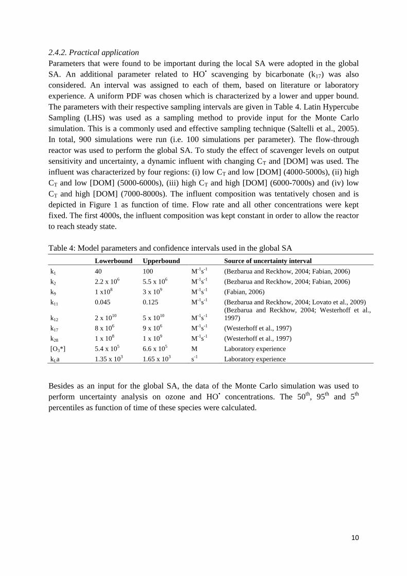
2.4.2. Practical application
Parameters that were found to be important during the local SA were adopted in the global
SA. An additional parameter related to HO• scavenging by bicarbonate (k17) was also
considered. An interval was assigned to each of them, based on literature or laboratory
experience. A uniform PDF was chosen which is characterized by a lower and upper bound.
The parameters with their respective sampling intervals are given in Table 4. Latin Hypercube
Sampling (LHS) was used as a sampling method to provide input for the Monte Carlo
simulation. This is a commonly used and effective sampling technique (Saltelli et al., 2005).
In total, 900 simulations were run (i.e. 100 simulations per parameter). The flow-through
reactor was used to perform the global SA. To study the effect of scavenger levels on output
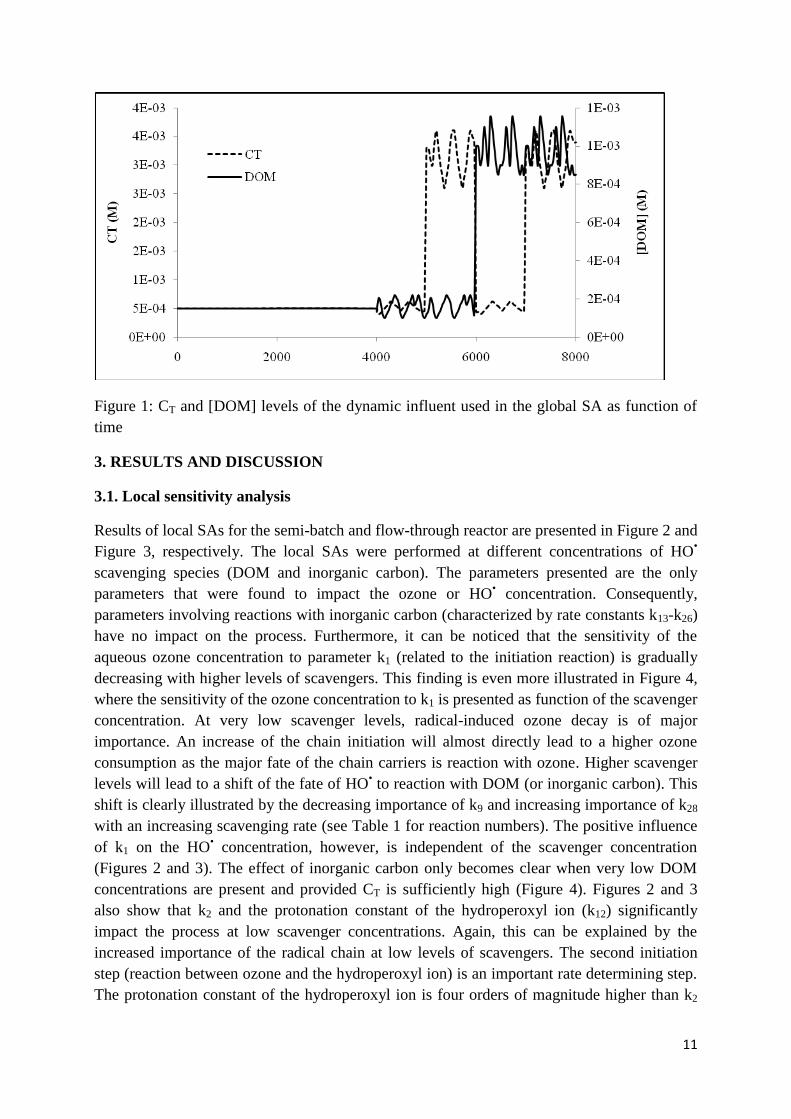
sensitivity and uncertainty, a dynamic influent with changing CT and [DOM] was used. The
influent was characterized by four regions: (i) low CT and low [DOM] (4000-5000s), (ii) high
CT and low [DOM] (5000-6000s), (iii) high CT and high [DOM] (6000-7000s) and (iv) low
CT and high [DOM] (7000-8000s). The influent composition was tentatively chosen and is
depicted in Figure 1 as function of time. Flow rate and all other concentrations were kept
fixed. The first 4000s, the influent composition was kept constant in order to allow the reactor
to reach steady state.
Table 4: Model parameters and confidence intervals used in the global SA
Lowerbound Upperbound Source of uncertainty interval
k1 40 100 M-1
s-1
(Bezbarua and Reckhow, 2004; Fabian, 2006)
k2 2.2 x 10⁶ 5.5 x 10
6 M
-1s
-1 (Bezbarua and Reckhow, 2004; Fabian, 2006)
k9 1 x10⁸ 3 x 10
9 M
-1s
-1 (Fabian, 2006)
k11 0.045 0.125 M-1
s-1
(Bezbarua and Reckhow, 2004; Lovato et al., 2009)
k12 2 x 10¹⁰
5 x 10¹⁰
M-1
s-1
(Bezbarua and Reckhow, 2004; Westerhoff et al.,
1997)
k17 8 x 10⁶ 9 x 10
6 M
-1s
-1 (Westerhoff et al., 1997)
k28 1 x 10⁸ 1 x 10
9 M
-1s
-1 (Westerhoff et al., 1997)
[O3*] 5.4 x 10⁵ 6.6 x 10
5 M Laboratory experience
kLa 1.35 x 10³ 1.65 x 10
3 s
-1 Laboratory experience
Besides as an input for the global SA, the data of the Monte Carlo simulation was used to
perform uncertainty analysis on ozone and HO• concentrations. The 50
th, 95
th and 5
th
percentiles as function of time of these species were calculated.
11
Figure 1: CT and [DOM] levels of the dynamic influent used in the global SA as function of
time
3. RESULTS AND DISCUSSION
3.1. Local sensitivity analysis
Results of local SAs for the semi-batch and flow-through reactor are presented in Figure 2 and
Figure 3, respectively. The local SAs were performed at different concentrations of HO•
scavenging species (DOM and inorganic carbon). The parameters presented are the only
parameters that were found to impact the ozone or HO• concentration. Consequently,
parameters involving reactions with inorganic carbon (characterized by rate constants k13-k26)
have no impact on the process. Furthermore, it can be noticed that the sensitivity of the
aqueous ozone concentration to parameter k1 (related to the initiation reaction) is gradually
decreasing with higher levels of scavengers. This finding is even more illustrated in Figure 4,
where the sensitivity of the ozone concentration to k1 is presented as function of the scavenger
concentration. At very low scavenger levels, radical-induced ozone decay is of major
importance. An increase of the chain initiation will almost directly lead to a higher ozone
consumption as the major fate of the chain carriers is reaction with ozone. Higher scavenger
levels will lead to a shift of the fate of HO• to reaction with DOM (or inorganic carbon). This
shift is clearly illustrated by the decreasing importance of k9 and increasing importance of k28
with an increasing scavenging rate (see Table 1 for reaction numbers). The positive influence
of k1 on the HO• concentration, however, is independent of the scavenger concentration
(Figures 2 and 3). The effect of inorganic carbon only becomes clear when very low DOM
concentrations are present and provided CT is sufficiently high (Figure 4). Figures 2 and 3
also show that k2 and the protonation constant of the hydroperoxyl ion (k12) significantly
impact the process at low scavenger concentrations. Again, this can be explained by the
increased importance of the radical chain at low levels of scavengers. The second initiation
step (reaction between ozone and the hydroperoxyl ion) is an important rate determining step.
The protonation constant of the hydroperoxyl ion is four orders of magnitude higher than k2
12
and hence, production of hydrogen peroxide will significantly slow down the chain initiation.
It is already recognized that the addition of hydrogen peroxide to enhance chain initiation is
only of value at high ozone and/or hydrogen peroxide concentrations, due to the slow
dissociation and initiation reactions (Buffle et al., 2006a).
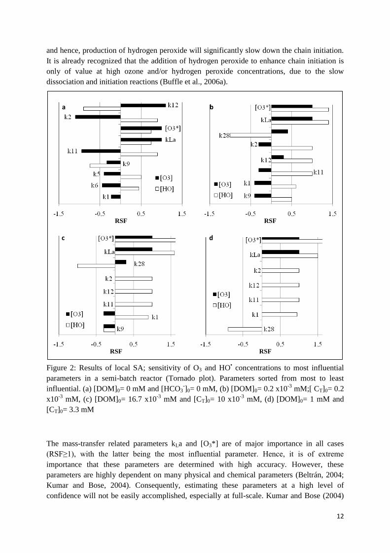
Figure 2: Results of local SA; sensitivity of O3 and HO• concentrations to most influential
parameters in a semi-batch reactor (Tornado plot). Parameters sorted from most to least
influential. (a) [DOM]0= 0 mM and [HCO3-]0= 0 mM, (b) [DOM]0= 0.2 x10
-3 mM;[ CT]0= 0.2
x10-3
mM, (c) [DOM]0= 16.7 x10⁻³
mM and [CT]0= 10 x10-3
mM, (d) [DOM]0= 1 mM and
[CT]0= 3.3 mM
The mass-transfer related parameters kLa and [O3*] are of major importance in all cases
(RSF≥1), with the latter being the most influential parameter. Hence, it is of extreme
importance that these parameters are determined with high accuracy. However, these
parameters are highly dependent on many physical and chemical parameters (Beltrán, 2004;
Kumar and Bose, 2004). Consequently, estimating these parameters at a high level of
confidence will not be easily accomplished, especially at full-scale. Kumar and Bose (2004)
RSF RSF
RSF RSF
a b
c d

13
in their study concluded that discrepancies between experimental and modeled ozone
concentrations were almost totally due to uncertainties in kLa and [O3*] and not due to effects
related to the mechanistic model under study.
Figure 3: Results of local SA; sensitivity of O3 and HO• concentrations to most influential
parameters in a flow-through reactor (Tornado plot). Parameters sorted from most to least
influential. (a) [DOM]0= 0 mM and [CT]0= 0 mM, (b) [DOM]0= 0.2 x10⁻³
mM;[ CT]0= 0.2
x10-3
mM, (c) [DOM]0= 16.7 x10⁻³
mM and [CT]0= 10 x10-3
mM, (d) [DOM]0= 1 mM and
[CT]0= 3.3 mM
a b
c d
RSF RSF
RSF RSF
14
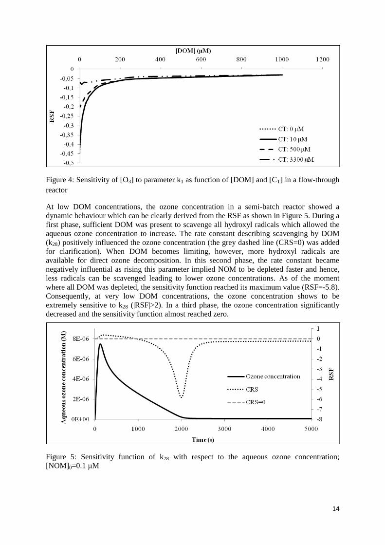
Figure 4: Sensitivity of [O3] to parameter k1 as function of [DOM] and [CT] in a flow-through
reactor
At low DOM concentrations, the ozone concentration in a semi-batch reactor showed a
dynamic behaviour which can be clearly derived from the RSF as shown in Figure 5. During a
first phase, sufficient DOM was present to scavenge all hydroxyl radicals which allowed the
aqueous ozone concentration to increase. The rate constant describing scavenging by DOM
(k28) positively influenced the ozone concentration (the grey dashed line (CRS=0) was added
for clarification). When DOM becomes limiting, however, more hydroxyl radicals are
available for direct ozone decomposition. In this second phase, the rate constant became
negatively influential as rising this parameter implied NOM to be depleted faster and hence,
less radicals can be scavenged leading to lower ozone concentrations. As of the moment
where all DOM was depleted, the sensitivity function reached its maximum value (RSF=-5.8).
Consequently, at very low DOM concentrations, the ozone concentration shows to be
extremely sensitive to k28 (|RSF|>2). In a third phase, the ozone concentration significantly
decreased and the sensitivity function almost reached zero.
Figure 5: Sensitivity function of k28 with respect to the aqueous ozone concentration;
[NOM]0=0.1 µM

15
The extreme importance of DOM at very low concentrations has some important practical
implications. Westerhoff et al. (1997) studied the SHB model using a batch reactor. Despite
the fact that Milli-Q (ultrapure) water was used, the authors considered the presence of
residual organic impurities with a concentration of 0.2 mg C L-1
(16.7 µM) (Westerhoff et al.,
1997). The reaction sequence was therefore extended with a simple HO• scavenging reaction
with a second order rate constant of 2 x 10⁸ M
-1s
-1. A satisfactory model prediction of the
ozone decomposition profile could be obtained. Lovato et al. (2009) used the SHB model to
describe ozone decomposition in a 11.5 L batch reactor at pH 4.8. The authors showed that
the SHB model in its original form severely overestimated the ozone decay (Lovato et al.,
2009). In order to obtain better fits, the model was modified. The reactor filled with ultrapure
water was, however, assumed to be totally free of residual impurities and in contrast to the
study of Westerhoff et al. (1997), the model did not account for these inhibiting substances.
Figure 6 shows the measured ozone data adopted from Lovato et al. (2009). The solid line
represents a simulation in which the water was considered to be free of impurities (analogous
to Lovato et al. (2009)). The dashed line is representing a simulation in which very low
concentrations of impurities (tentatively chosen) were considered ([DOM]0=0.1 µM, CT=10
µM). It can be clearly observed from this figure that extremely low levels of impurities have a
significant impact on model predictions. Consequently, impurities should always be
considered in ultrapure water systems.
Figure 6: The effect of low levels of impurities on the modelled ozone concentration;
experimental data points were adopted from Lovato et al. (2009)
3.2. Global sensitivity analysis
Results of the global SA for the ozone and HO• concentration are presented in Figure 7. The
tornado plots are comparable to those of the local SA conducted in the presence of scavengers
(Figure 3). Therefore, only the most remarkable differences will be discussed in this section.
16
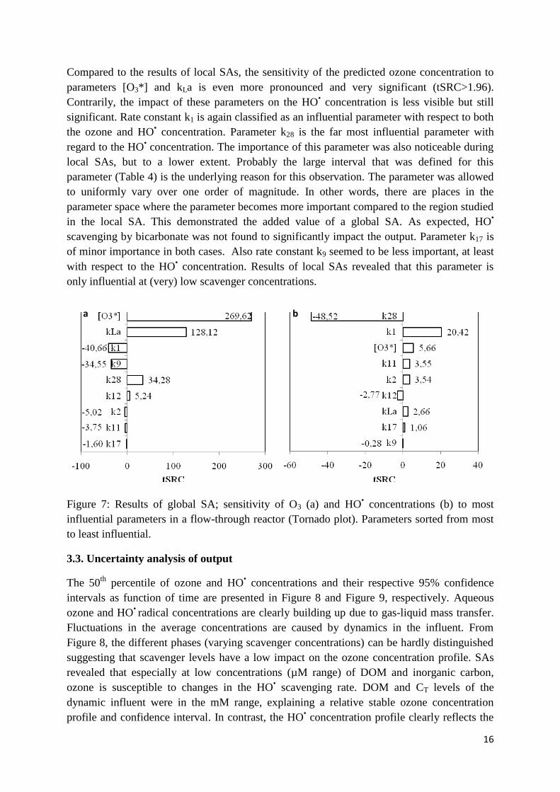
Compared to the results of local SAs, the sensitivity of the predicted ozone concentration to
parameters [O3*] and kLa is even more pronounced and very significant (tSRC>1.96).
Contrarily, the impact of these parameters on the HO• concentration is less visible but still
significant. Rate constant k1 is again classified as an influential parameter with respect to both
the ozone and HO• concentration. Parameter k28 is the far most influential parameter with
regard to the HO• concentration. The importance of this parameter was also noticeable during
local SAs, but to a lower extent. Probably the large interval that was defined for this
parameter (Table 4) is the underlying reason for this observation. The parameter was allowed
to uniformly vary over one order of magnitude. In other words, there are places in the
parameter space where the parameter becomes more important compared to the region studied
in the local SA. This demonstrated the added value of a global SA. As expected, HO•
scavenging by bicarbonate was not found to significantly impact the output. Parameter k17 is
of minor importance in both cases. Also rate constant k9 seemed to be less important, at least
with respect to the HO• concentration. Results of local SAs revealed that this parameter is
only influential at (very) low scavenger concentrations.
Figure 7: Results of global SA; sensitivity of O3 (a) and HO• concentrations (b) to most
influential parameters in a flow-through reactor (Tornado plot). Parameters sorted from most
to least influential.
3.3. Uncertainty analysis of output
The 50th
percentile of ozone and HO• concentrations and their respective 95% confidence
intervals as function of time are presented in Figure 8 and Figure 9, respectively. Aqueous
ozone and HO• radical concentrations are clearly building up due to gas-liquid mass transfer.
Fluctuations in the average concentrations are caused by dynamics in the influent. From
Figure 8, the different phases (varying scavenger concentrations) can be hardly distinguished
suggesting that scavenger levels have a low impact on the ozone concentration profile. SAs
revealed that especially at low concentrations (µM range) of DOM and inorganic carbon,
ozone is susceptible to changes in the HO• scavenging rate. DOM and CT levels of the
dynamic influent were in the mM range, explaining a relative stable ozone concentration
profile and confidence interval. In contrast, the HO• concentration profile clearly reflects the
a b

17
different phases. Uncertainty significantly decreases from 5000s as more inorganic carbon is
entering the reactor. The average HO• concentration, however, only significantly decreases
when the DOM level is increased (6000s). From this moment, a drastic reduction of the
uncertainty interval occurs.
Figure 8: 50th
percentile of predicted ozone concentration (solid line) with 95% confidence
interval (dashed lines) as function of time; plot derived from 900 Monte Carlo runs
Figure 9: 50th
percentile of predicted HO• concentration (solid line) with 95% confidence
interval (dashed lines) as function of time; plot derived from 900 Monte Carlo runs
Based on the global SA, most of the uncertainty in HO• concentration is caused by a not well
defined rate constant describing scavenging by DOM (k28). This illustrates the importance of
including more detailed DOM reaction sequences in future models in order to reduce this
uncertainty. A reliable estimation of HO• exposure is of vital importance for DOM moieties
that slowly react with ozone and hence, are primarly removed by HO• induced oxidation
(Neumann et al., 2009; Zimmermann et al., 2011).

18
4. CONCLUSIONS
In this study, the extensive SBH model consisting of a set of elementary reactions describing
aqueous ozone decomposition was investigated in detail by means of sensitivity analysis. The
model was extended with a simple equation describing hydroxyl radical scavenging by DOM
to study the effect of varying scavenger concentrations. Local SAs revealed that only seven of
the twenty-eight first and second order rate constants showed to impact ozone and HO•
concentrations. Processes involving HO• scavenging by inorganic carbon were of minor
importance. The effect of inorganic carbon only became clear when very low DOM
concentrations were present and provided CT was sufficiently high. Mass-transfer related
parameters kLa and [O3*] were of major importance in all cases. Hence, it is of extreme
importance that these parameters are determined with high accuracy, which is a rather
difficult task given the many physical and chemical parameters affecting them. It was shown
that the aqueous ozone concentration is extremely sensitive to parameters involving DOM at
very low scavenger concentrations. Hence, impurities should always be considered in models,
even in ultrapure water systems.
Results of a global SA were to a high extent comparable to these of local SAs. The
importance of the mass-transfer related parameters was even more pronounced. Furthermore,
the global SA revealed that a detailed description of reactions involving DOM is of vital
importance as their related parameters seem to be very important. Uncertainty analysis
showed that especially the HO• concentration is susceptible to variations in influent
composition. The uncertainty regarding this species significantly reduced with increasing
levels of scavengers and especially DOM.
It was shown in this study that simplification of the elementary radical scheme should be
considered. For example, it is questionable if inorganic reactions should be included when
DOM levels are sufficiently high. Additionally, some dissociation reactions might be
discarded if the model is used within a predefined pH range. On the other hand, a model
extension with regard to reactions involving DOM should be considered in order to improve
the applicability of future wastewater ozonation models. It should, however, be highlighted
that in this study DOM was only considered as inhibitor. Direct reactions with ozone,
promoting and initiating properties of DOM were not included. Hence, this study is a detailed
analysis of the SHB model, but did not include all important reaction steps of DOM. This will
be an important issue in future research.
5. ACKNOLEDGEMENTS
This research was partially funded by a University College West Flanders PhD research grant
and is in close cooperation with the Veg-i-Trade FP7-KBBE-2009-3 project.

19
6. REFERENCES
Audenaert, W. T. M., Callewaert, M., Nopens, I., Cromphout, J., Vanhoucke, R., Dumoulin, A., Dejans, P., and Van Hulle, S. W. H. (2010). Full-scale modelling of an ozone reactor for drinking water treatment. Chemical Engineering Journal 157, 551-557.
Audenaert, W. T. M., Vermeersch, Y., Van Hulle, S. W. H., Dejans, P., Dumoulin, A., and Nopens, I. (2011). Application of a mechanistic UV/hydrogen peroxide model at full-scale: Sensitivity analysis, calibration and performance evaluation. Chemical Engineering Journal 171, 113-126.
Beltrán, F. J. (2004). "Ozone Reaction Kinetics for Water and Wastewater Systems," CRC Press, Florida, USA.
Bezbarua, B. K., and Reckhow, D. A. (2004). Modification of the standard neutral ozone decomposition model. Ozone-Science & Engineering 26, 345-357.
Buffle, M. O., Schumacher, J., Meylan, S., Jekel, M., and von Gunten, U. (2006a). Ozonation and advanced oxidation of wastewater: Effect of O-3 dose, pH, DOM and HO center dot-scavengers on ozone decomposition and HO center dot generation. Ozone-Science & Engineering 28, 247-259.
Buffle, M. O., Schumacher, J., Salhi, E., Jekel, M., and von Gunten, U. (2006b). Measurement of the initial phase of ozone decomposition in water and wastewater by means of a continuous quench-flow system: Application to disinfection and pharmaceutical oxidation. Water Research 40, 1884-1894.
Buhler, R. E., Staehelin, J., and Hoigne, J. (1984). OZONE DECOMPOSITION IN WATER STUDIED BY PULSE-RADIOLYSIS .1. HO2/O2-AND HO3/O3- AS INTERMEDIATES. Journal of Physical Chemistry 88, 2560-2564.
Elovitz, M. S., and von Gunten, U. (1999). Hydroxyl radical ozone ratios during ozonation processes. I-The R-ct concept. Ozone-Science & Engineering 21, 239-260.
Fabian, I. (2006). Reactive intermediates in aqueous ozone decomposition: A mechanistic approach. Pure and Applied Chemistry 78, 1559-1570.
Henze, M., Gujer, W., Mino, T., and van Loodsrecht, M. (2000). "Activated sludge models ASM1, ASM2, ASM2d and ASM3," IWA Publishing, London.
Hindmarsh, A. C., and Petzold, L. R. (1995). Algorithms and software for ordinary differential equations and differential-algebraic equations. Computers in Physics 9, 148-155.
Kumar, R., and Bose, P. (2004). Development and experimental validation of the model of a continuous-flow countercurrent ozone contactor. Industrial & Engineering Chemistry Research 43, 1418-1429.
Lovato, M. E., Martin, C. A., and Cassano, A. E. (2009). A reaction kinetic model for ozone decomposition in aqueous media valid for neutral and acidic pH. Chemical Engineering Journal 146, 486-497.
Lovato, M. E., Martín, C. A., and Cassano, A. E. (2011). A reaction–reactor model for O3 and UVC radiation degradation of dichloroacetic acid: The kinetics of three parallel reactions. Chemical Engineering Journal 171, 474-489.
Neumann, M. B., Gujer, W., and von Gunten, U. (2009). Global sensitivity analysis for model-based prediction of oxidative micropollutant transformation during drinking water treatment. Water Research 43, 997-1004.
Saltelli, A., Ratto, M., Tarantola, S., and Campolongo, F. (2005). Sensitivity analysis for chemical models. Chemical Reviews 105, 2811-2827.
Staehelin, J., Buhler, R. E., and Hoigne, J. (1984). OZONE DECOMPOSITION IN WATER STUDIED BY PULSE-RADIOLYSIS .2. OH AND HO4 AS CHAIN INTERMEDIATES. Journal of Physical Chemistry 88, 5999-6004.
Van Geluwe, S., Braeken, L., and Van der Bruggen, B. (2011). Ozone oxidation for the alleviation of membrane fouling by natural organic matter: A review. Water Research 45, 3551-3570.
20
Vanhooren, H., De Pauw, D., and Vanrolleghem, P. A. (2003). Induction of denitrification in a pilot-scale trickling filter by adding nitrate at high loading rate. Water Science and Technology 47, 61-68.
Westerhoff, P., Aiken, G., Amy, G., and Debroux, J. (1999). Relationships between the structure of natural organic matter and its reactivity towards molecular ozone and hydroxyl radicals. Water Research 33, 2265-2276.
Westerhoff, P., Mezyk, S. P., Cooper, W. J., and Minakata, D. (2007). Electron pulse radiolysis determination of hydroxyl radical rate constants with Suwannee river fulvic acid and other dissolved organic matter isolates. Environmental Science & Technology 41, 4640-4646.
Westerhoff, P., Song, R., Amy, G., and Minear, R. (1997). Applications of ozone decomposition models. Ozone-Science & Engineering 19, 55-73.
Zimmermann, S. G., Wittenwiler, M., Hollender, J., Krauss, M., Ort, C., Siegrist, H., and von Gunten, U. (2011). Kinetic assessment and modeling of an ozonation step for full-scale municipal wastewater treatment: Micropollutant oxidation, by-product formation and disinfection. Water Research 45, 605-617.
21
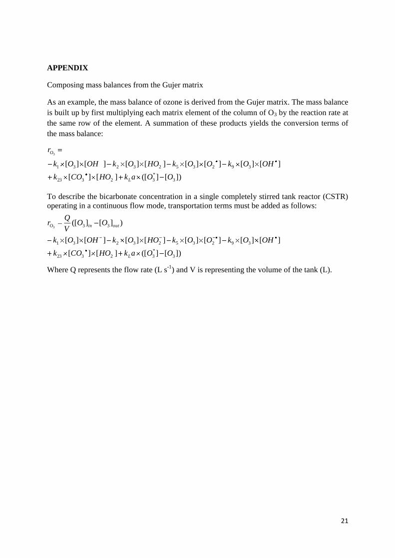
APPENDIX
Composing mass balances from the Gujer matrix
As an example, the mass balance of ozone is derived from the Gujer matrix. The mass balance
is built up by first multiplying each matrix element of the column of O3 by the reaction rate at
the same row of the element. A summation of these products yields the conversion terms of
the mass balance:
To describe the bicarbonate concentration in a single completely stirred tank reactor (CSTR)
operating in a continuous flow mode, transportation terms must be added as follows:
Where Q represents the flow rate (L s-1
) and V is representing the volume of the tank (L).
])[]([][][
][][][][][][][][
3
*
32323
3923523231
3
OOakHOCOk
OHOkOOkHOOkOHOk
r
L
O
])[]([][][
][][][][][][][][
)][]([
3
*
32323
3923523231
333
OOakHOCOk
OHOkOOkHOOkOHOk
OOV
Qr
L
outinO