InflationInflationInflationInflation

Andrei Linde Andrei Linde

Lecture 2

Inflation as a theory of a Inflation as a theory of a harmonic oscillatorharmonic oscillator Inflation as a theory of a Inflation as a theory of a harmonic oscillatorharmonic oscillator

Eternal InflationEternal Inflation

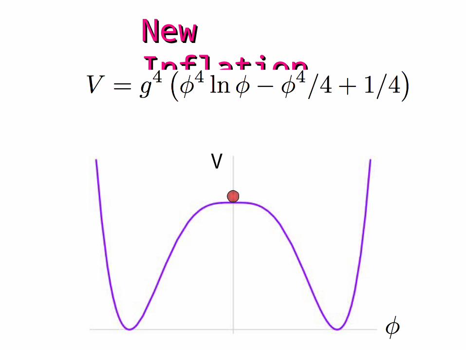
New New InflationInflationNew New InflationInflation

V

Hybrid Hybrid InflationInflation Hybrid Hybrid InflationInflation

Warm-up:Warm-up: Dynamics of Dynamics of spontaneous symmetry breakingspontaneous symmetry breakingWarm-up:Warm-up: Dynamics of Dynamics of spontaneous symmetry breakingspontaneous symmetry breaking

φ

V

How many oscillations does the field distribution make before it relaxes near the minimum of the potential V ?

Answer:Answer: 1 1

oscillationoscillation

Answer:Answer: 1 1

oscillationoscillation

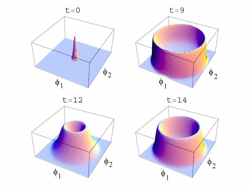
All quantum fluctuations with k < m grow exponentially:

When they reach the minimum of the potential, the energy of the field gradients becomes comparable with its initial potential energy.

Not much is left for the oscillations; the process of spontaneous symmetry breaking is basically over in a single oscillation of the field distribution.

After hybrid After hybrid InflationInflation After hybrid After hybrid InflationInflation

Inflating Inflating topological defects topological defects in new inflation in new inflation

Inflating Inflating topological defects topological defects in new inflation in new inflation

V

and expansion of space

During inflation we have two competing processes: growth of the field

For H >> m, the value of the field in a vicinity of a topological defect exponentially decreases, and the total volume of space containing small values of the field exponentially grows.

Topological inflation, A.L. 1994, Vilenkin 1994

Small quantum fluctuations of the scalar field freeze on the top of the flattened distribution of the scalar field. This creates new pairs of points where the scalar field vanishes, i.e. new pairs of topological defects. They do not annihilate because the distance between them exponentially grows.Then quantum fluctuations in a vicinity of each new inflating monopole produce new pairs of inflating monopoles.

Thus, the total volume of space near inflating domain walls (strings, monopoles) grows exponentially, despite the ongoing process of spontaneous symmetry breaking.

Inflating `t Hooft - Polyakov monopoles serve as indestructible seeds for the universe creation.

If inflation begins inside one such monopole, it continues forever, and creates an infinitely large fractal distribution of eternally inflating monopoles.

x

This process continues, and eventually the universe becomes populated by inhomogeneous scalar field. Its energy takes different values in different parts of the universe. These inhomogeneities are responsible for the formation of galaxies.Sometimes these fluctuations are so large that they substantially increase the value of the scalar field in some parts of the universe. Then inflation in these parts of the universe occurs again and again. In other words, the process of inflation becomes eternal.

We will illustrate it now by computer simulation of this process.

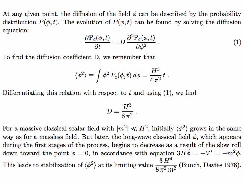
Inflationary perturbations and Inflationary perturbations and Brownian motionBrownian motionInflationary perturbations and Inflationary perturbations and Brownian motionBrownian motionPerturbations of the massless scalar field are

frozen each time when their wavelength becomes greater than the size of the horizon, or, equivalently, when their momentum k becomes smaller than H.Each time t = H-1 the perturbations with H < k < e H become frozen. Since the only dimensional parameter describing this process is H, it is clear that the average amplitude of the perturbations frozen during this time interval is proportional to H. A detailed calculation shows that

This process repeats each time t = H-1 , but the sign of each time can be different, like in the Brownian motion. Therefore the typical amplitude of accumulated quantum fluctuations can be estimated as

Amplitude of perturbations Amplitude of perturbations of metricof metricAmplitude of perturbations Amplitude of perturbations of metricof metric

In fact, there are two different diffusion equations: The first one (Kolmogorov forward equation) describes the probability to find the field if the evolution starts from the initial field . The second equation (Kolmogorov backward equation) describes the probability that the initial value of the field is given by if the evolution eventually brings the field to its present value .

For the stationary regime the combined solution of these two equations is given by

The first of these two terms is the square of the tunneling wave function of the universe, describing the probability of initial conditions. The second term is the square of the Hartle-Hawking wave function describing the ground state of the universe.

Eternal Eternal Chaotic InflationChaotic Inflation Eternal Eternal Chaotic InflationChaotic Inflation

Eternal Eternal Chaotic InflationChaotic Inflation Eternal Eternal Chaotic InflationChaotic Inflation

Generation of Quantum Generation of Quantum

FluctuationsFluctuations

Generation of Quantum Generation of Quantum

FluctuationsFluctuations

QuickTime™ and a decompressor

are needed to see this picture.

From the Universe to the From the Universe to the MultiverseMultiverseFrom the Universe to the From the Universe to the MultiverseMultiverseIn realistic theories of elementary particles there are many scalar fields, and their potential energy has many different minima. Each minimum corresponds to different masses of particles and different laws of their interactions.

Quantum fluctuations during eternal inflation can bring the scalar fields to different minima in different exponentially large parts of the universe. The universe becomes divided into many exponentially large parts with different laws of physics operating in each of them. (In our computer simulations we will show them by using different colors.)

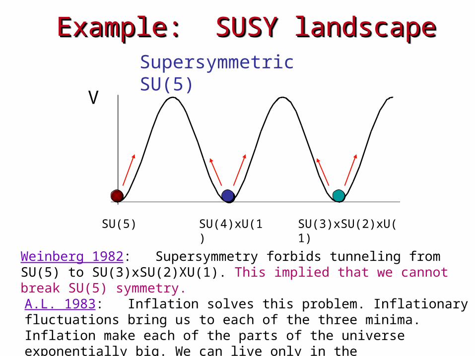
Example: SUSY landscapeExample: SUSY landscape Example: SUSY landscapeExample: SUSY landscape

V

SU(5) SU(3)xSU(2)xU(1)

SU(4)xU(1)

Weinberg 1982: Supersymmetry forbids tunneling from SU(5) to SU(3)xSU(2)XU(1). This implied that we cannot break SU(5) symmetry. A.L. 1983: Inflation solves this problem. Inflationary fluctuations bring us to each of the three minima. Inflation make each of the parts of the universe exponentially big. We can live only in the SU(3)xSU(2)xU(1) minimum.

Supersymmetric SU(5)

Kandinsky Kandinsky

UniverseUniverse Kandinsky Kandinsky

UniverseUniverse

Genetic code of the Genetic code of the UniverseUniverse

Genetic code of the Genetic code of the UniverseUniverse One may have just one fundamental law of

physics, like a single genetic code for the whole Universe. However, this law may have different realizations. For example, water can be liquid, solid or gas. In elementary particle physics, the effective laws of physics depend on the values of the scalar fields, on compactification and fluxes.Quantum fluctuations during inflation can take scalar fields from one minimum of their potential energy to another, altering its genetic code. Once it happens in a small part of the universe, inflation makes this part exponentially big. This is the This is the

cosmological mutation cosmological mutation mechanismmechanism

This is the This is the cosmological mutation cosmological mutation

mechanismmechanism

Populating the Populating the

LandscapeLandscape

Populating the Populating the

LandscapeLandscape

QuickTime™ and a decompressor

are needed to see this picture.

Landscape of eternal inflation Landscape of eternal inflation