infinite svm: a dp mixture of large-margin kernel...
TRANSCRIPT

[70240413 Statistical Machine Learning, Spring, 2015]
http://bigml.cs.tsinghua.edu.cn/~jun
State Key Lab of Intelligent Technology & Systems
Tsinghua University
June 2, 2015
Deep Learning

Why going deep?
Data are often high-dimensional.
There is a huge amount of structure in the data, but the structure is too complicated to be represented by a simple model.
Insufficient depth can require more computational elementsthan architectures whose depth matches the task.
Deep nets provide simpler but more descriptive models of many problems.

Microsoft’s speech recognition system
http://v.youku.com/v_show/id_XNDc0MDY4ODI0.html
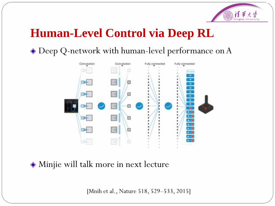
Human-Level Control via Deep RL
Deep Q-network with human-level performance on A
Minjie will talk more in next lecture
[Mnih et al., Nature 518, 529–533, 2015]

MIT 10 Breakthrough Tech 2013
http://www.technologyreview.com/featuredstory/513696/deep-learning/

Deep Learning in industry
Driverless car Face identification Speech recognition Web search
…
…

Deep Learning Models

How brains seem to do computing?
The business end of this is made of lots of these joined in networks like this
Much of our own “computations” are performed in/by this network
Learning occurs by changing the effectiveness of the synapses so that the
influence of one neuron on another changes

History of neural networks

History of neural networks

Model of a neuron
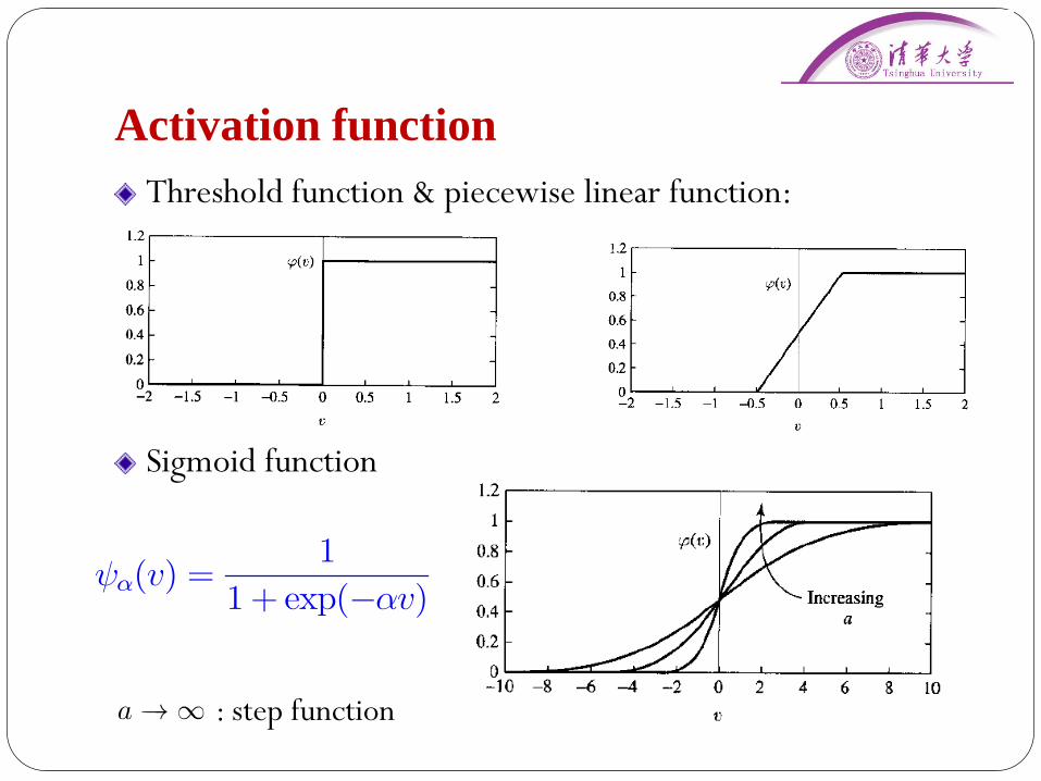
Activation function
Threshold function & piecewise linear function:
Sigmoid function
î(v) =1
1 + exp(¡®v)
: step function
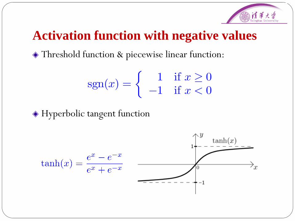
Activation function with negative values
Threshold function & piecewise linear function:
Hyperbolic tangent function
sgn(x) =
½1 if x ¸ 0
¡1 if x < 0

McCulloch & Pitts’s Artificial Neuron
The first model of artificial neurons in 1943
Activation function: a threshold function

Network Architecture
Feedforward networks
Recurrent networksInput layer
Hidden layer
Output layer
Output
Input

Learning Paradigms
Unsupervised learning (learning without a teacher)
Example: clustering

Learning Paradigms
Supervised Learning (learning with a teacher)
For example, classification: learns a separation plane
Learning Rules
Error-correction learning
Competitive learning
Hebbian learning
Boltzmann learning
Memory-base learning
Nearest neighbor, radial-basis function network
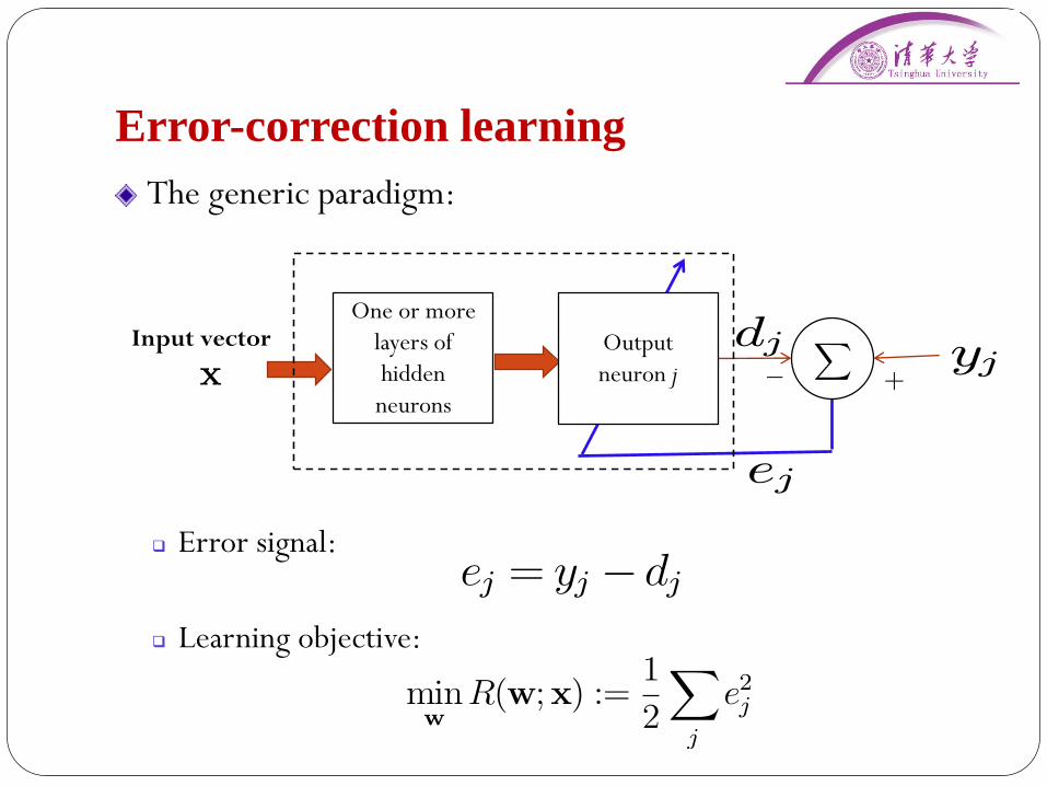
Error-correction learning
The generic paradigm:
Error signal:
Learning objective:
One or more
layers of
hidden
neurons
Input vector
+¡yjx
dj
ej = yj ¡dj
Output
neuron j
ej
minw
R(w;x) :=1
2
X
j
e2j

Example: Perceptron
One-layer feedforward network based on error-correction learning (no hidden layer):
Current output (at iteration t):
Update rule (exercise?):
wjt+1 = w
jt +´(yj ¡dj)x
dj = (wjt)>x

Perceptron for classification
Consider a single output neuron
Binary labels:
Output function:
Apply the error-correction learning rule, we get … (next
slide)
y 2 f+1;¡1g
d = sgn w>t x

Perceptron for Classification
Set and t=1; scale all examples to have length 1
(doesn’t affect which side of the plane they are on)
Given example x, predict positive iff
If a mistake, update as follows
Mistake on positive:
Mistake on negative:
w1 = 0
w>t x > 0
wt+1 Ã wt + ´tx
wt+1 Ãwt ¡ t́x
t à t + 1
wtwt wt+1

Convergence Theorem
For linearly separable case, the perceptron algorithm will
converge in a finite number of steps

Mistake Bound
Theorem:
Let be a sequence of labeled examples consistent with a linear
threshold function , where is a unit-length vector.
The number of mistakes made by the online Perceptron algorithm is at
most , where
i.e.: if we scale examples to have length 1, then is the minimum
distance of any example to the plane
is often called the “margin” of ; the quantity is the cosine
of the angle between and
w>¤ x > 0
Sw¤
(1=°)2
° = minx2S
jw>¤ xj
kxk
°
w>¤ x = 0
° w¤w>¤ x
kxkw¤x

Deep Nets
Multi-layer Perceptron
CNN
Auto-encoder
RBM
Deep belief nets
Deep recurrent nets

XOR Problem
Single-layer perceptron can’t solve the problem

XOR Problem
A network with 1-layer of 2 neurons works for XOR:
threshold activation function
Many alternative networks exist (not layered)

Multilayer Perceptrons
Computatonal limitations of single-layer Perceptron by
Minsky & Papert (1969)
Multilayer Perceptrons:
Multilayer feedforward networks with an error-correction
learning algorithm, known as error back-propagation
A generalization of single-layer percetron to allow nonlinearity

Backpropagation
Learning as loss minimization
Learning with gradient descent
Input layer
Hidden layer
Output layer
y1 yK
w1
w2
wL
ej = yj ¡dj
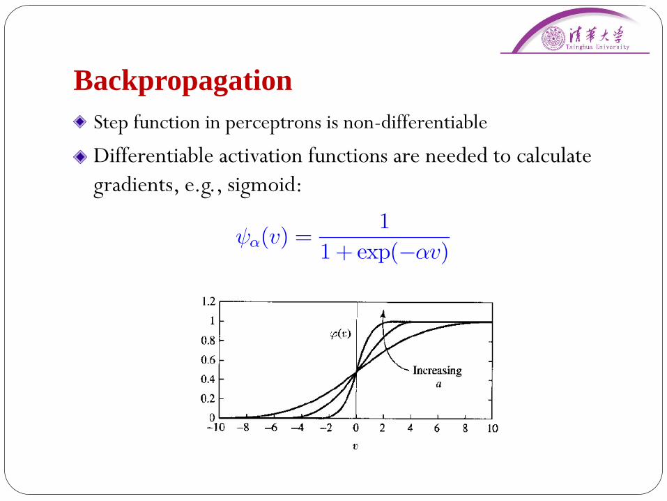
Backpropagation
Step function in perceptrons is non-differentiable
Differentiable activation functions are needed to calculate
gradients, e.g., sigmoid:
î(v) =1
1 + exp(¡®v)

Backpropagation
Derivative of a sigmoid function ( )
Notice about the small scale of the gradient
Gradient vanishing issue
Many other activation functions examined
rvÃ(v) =e¡v
(1 + e¡v)2= Ã(v)(1¡ Ã(v))
® = 1

Gradient computation at output layer
Output neurons are separate:
Input layer
Hidden layer
Output layer
y1 yK
w1
w2
wL
Assume this part is fixed
f1(x) fM (x)f2(x)

Gradient computation at output layer
Signal flow:
ej
yj
djX
vjÃ(¢) ¡
+
wj1
wj2
wjM
...
f1(x)
fM (x)
...
f2(x)
vj = w>j f(x) dj = Ã(vj) ej = yj ¡dj
Rj =1
2e2j
rwjiR =
@Rj
@ej
@ej
@dj
@dj
@vj
@vj
@wji
= ej ¢ (¡1) ¢ Ã0(vj) ¢ fi(x)
= ¡ejÃ0(vj)fi(x)R =
1
2
X
j
e2j
±j = ¡@R
@vjLocal gradient:
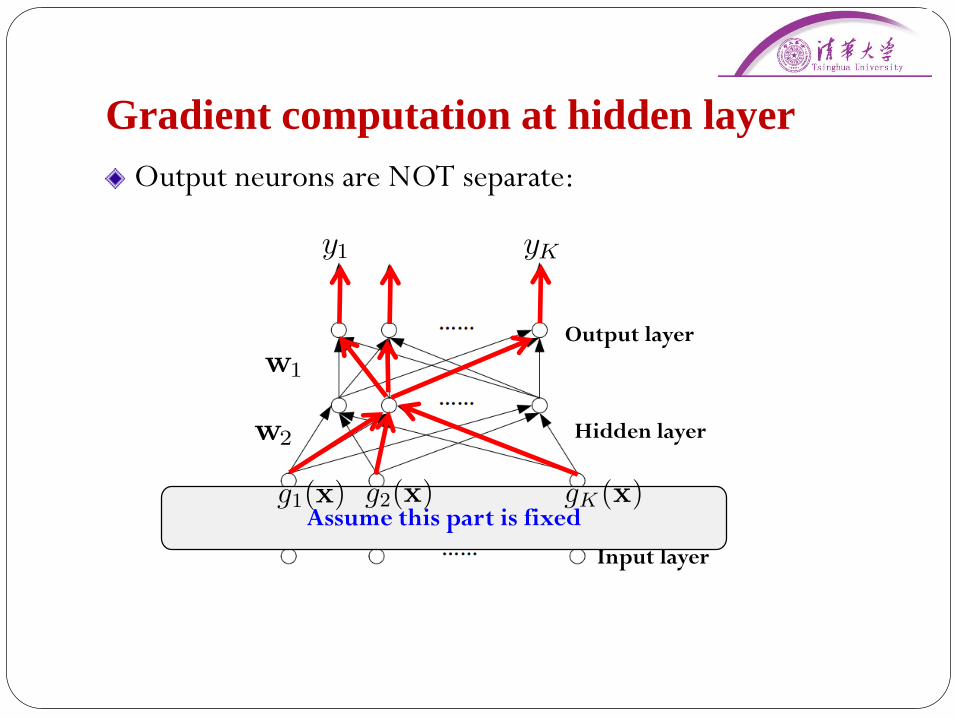
Gradient computation at hidden layer
Output neurons are NOT separate:
Input layer
Hidden layer
Output layer
y1 yK
w1
w2
wL Assume this part is fixedg1(x) gK (x)g2(x)

Gradient computation at hidden layer
ej
yj
djX
vjÃ(¢) ¡
+
wj1
wji
wjM
...
f1
fM
...
fi
vj = w>j f dj = Ã(vj) ej = yj ¡dj
Rj =1
2e2j
rw0ikR =
X
j
@Rj
@ej
@ej
@dj
@dj
@vj
@vj
@fi
@fi
@vi
@vi
@w0ik
= ¡X
j
ejÃ0(vj)wjiÃ
0(vi)gk(x)
= ¡X
j
±jwjiÃ0(vi)gk(x)
w0i1
w0i2
w0iK
...
viÃ(¢)
g1(x)
gK (x)
g2(x)
fi = Ã(vi)vi = (w0i)>g
R =1
2
X
j
e2j
±i = ¡@R
@vi
Local gradient:

Back-propagation formula
The update rule of local gradients:
for hidden neuron i:
Flow of error signal:
±i = Ã0(vi)X
j
±jwji
Only depends on the activation function at hidden neuron i
e1
ej
eJ
...
...
±1
±j
±J
...
...
±i
Ã0(v1)
Ã0(v2)
Ã0(vJ)
w1i
wji
wJiHidden
layer
Output layer

Back-propagation formula
The update rule of weights:
Output neuron:
Hidden neuron:
¢wji = ¸ ¢ ±j ¢ fi(x)
¢w0ik = ¸ ¢ ±i ¢ gk(x)
0
@Weight
correction
¢wji
1
A =
0
@learning
rate
¸
1
A ¢
0
@local
gradient
±j
1
A ¢
0
@input signal
of neuron j
vi
1
A

Two Passes of Computation
Forward pass
Weights fixed
Start at the first hidden layer
Compute the output of each neuron
End at output layer
Backward pass
Start at the output layer
Pass error signal backward through the network
Compute local gradients

Stopping Criterion
No general rules
Some reasonable heuristics:
The norm of gradient is small enough
The number of iterations is larger than a threshold
The training error is stable
…
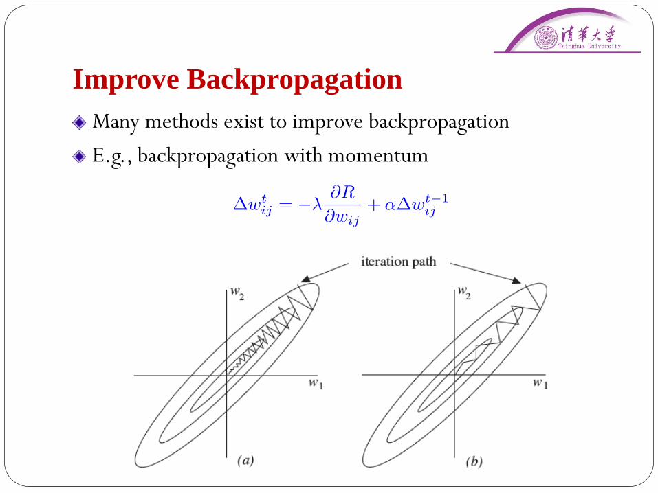
Improve Backpropagation
Many methods exist to improve backpropagation
E.g., backpropagation with momentum
¢wtij = ¡¸
@R
@wij
+ ®¢wt¡1ij
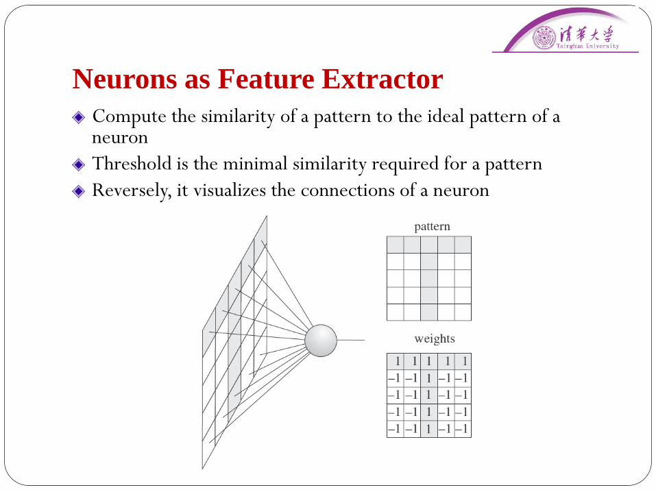
Neurons as Feature Extractor
Compute the similarity of a pattern to the ideal pattern of a neuron
Threshold is the minimal similarity required for a pattern
Reversely, it visualizes the connections of a neuron

Vanishing gradient problem
The gradient can decrease exponentially during back-prop
Solutions:
Pre-training + fine tuning
Rectifier neurons (sparse gradients)
Ref:
Gradient flow in recurrent nets: the difficulty of learning long-term dependencies. Hochreiter, Bengio, & Frasconi, 2001

Deep Rectifier NetsSparse representations without gradient vanishing
Non-linearity comes from the path selection Only a subset of neurons are active for a given input
Can been seen as a model with an exponential number of linear models that share weights
[Deep sparse rectifier neural networks. Glorot, Bordes, & Bengio, 2011]
CNN
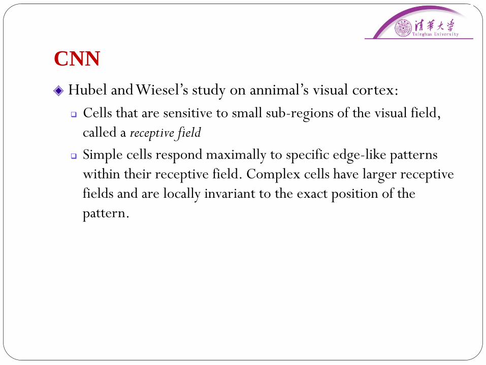
Hubel and Wiesel’s study on annimal’s visual cortex:
Cells that are sensitive to small sub-regions of the visual field,
called a receptive field
Simple cells respond maximally to specific edge-like patterns
within their receptive field. Complex cells have larger receptive
fields and are locally invariant to the exact position of the
pattern.

Convolutional Neural Networks
Sparse local connections (spatially contiguous receptive
fields)
Shared weights: each filter is replicated across the entire
visual field, forming a feature map

CNN
Each layer has multiple feature maps
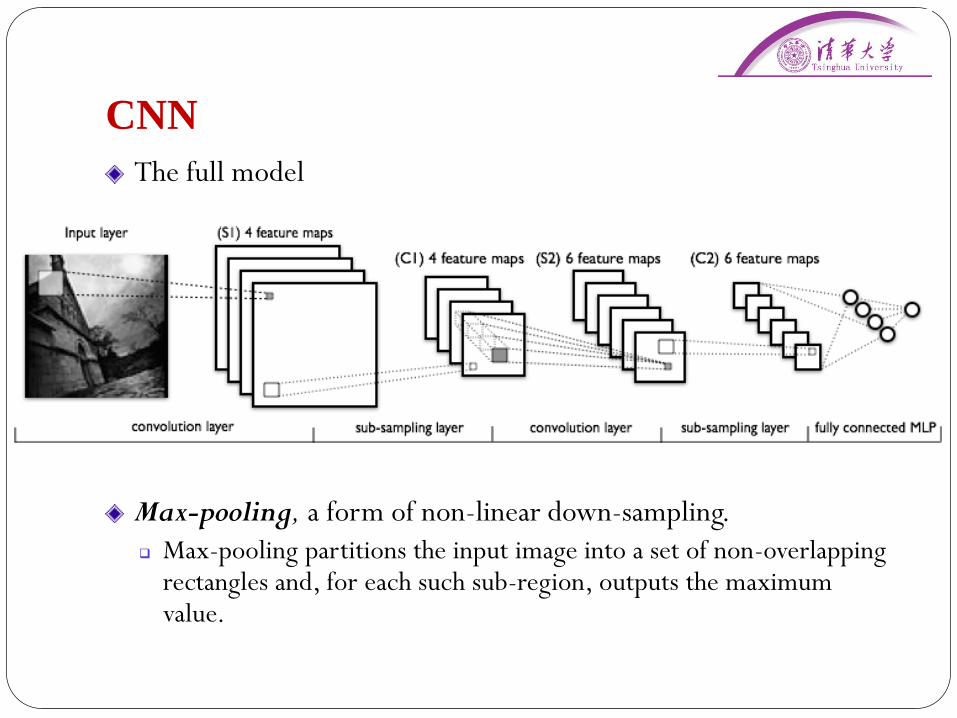
CNN
The full model
Max-pooling, a form of non-linear down-sampling.
Max-pooling partitions the input image into a set of non-overlapping rectangles and, for each such sub-region, outputs the maximum value.

Example: CNN for image classification
Network dimension: 150,528(input)-253,440–186,624–64,896–64,896–43,264–4096–4096–1000(output) In total: 60 million parameters
Task: classify 1.2 million high-resolution images in the ImageNetLSVRC-2010 contest into the 1000 different classes
Results: state-of-the-art accuracy on ImageNet
Krizhevsky, Sutskever and Hinton, NIPS, 2012

Issues with CNN
Computing the activations of a single convolutional filter is
much more expensive than with traditional MLPs
Many tuning parameters
# of filters:
Model complexity issue (overfitting vs underfitting)
Filter shape:
the right level of “granularity” in order to create abstractions at the proper
scale, given a particular dataset
Usually 5x5 for MNIST at 1st layer
Max-pooling shape:
typical: 2x2; maybe 4x4 for large images

Auto-Encoder
Encoder: (a distributed code)
Decoder:
Minimize reconstruction error
Connection to PCA
PCA is linear projection, which Auto-Encoder is nonlinear
Stacking PCA with nonlinear processing may perform as well (Ma Yi’s work)
Denoising Auto-Encoder
A stochastic version with corrupted noise to discover more robust features
E.g., randomly set some inputs to zero

Left: no noise; right: 30 percent noise
Deep Generative Models

Stochastic Binary Units
Each unit has a state of 0 or 1
The probability of turning on is determined by

Generative Models
Directed acyclic graph with
stochastic binary units is termed
Sigmoid Belief Net (Radford
Neal, 1992)
Undirected graph with stochastic
binary units is termed Boltzmann
Machine (Hinton & Sejnowski,
1983)
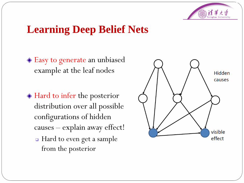
Learning Deep Belief Nets
Easy to generate an unbiased
example at the leaf nodes
Hard to infer the posterior
distribution over all possible
configurations of hidden
causes – explain away effect!
Hard to even get a sample
from the posterior
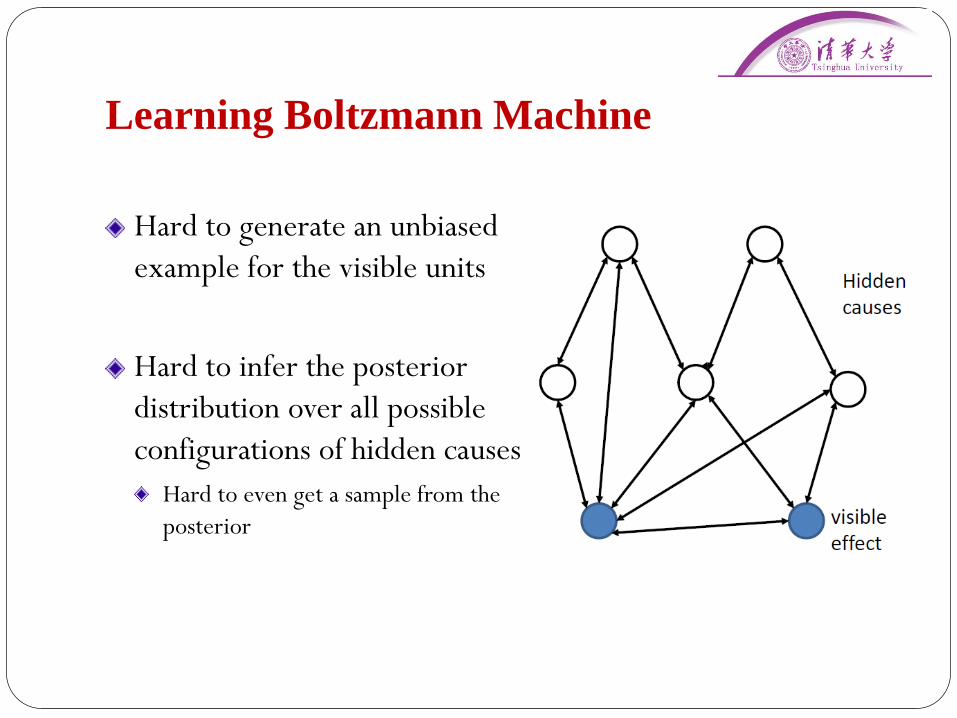
Learning Boltzmann Machine
Hard to generate an unbiased
example for the visible units
Hard to infer the posterior
distribution over all possible
configurations of hidden causes
Hard to even get a sample from the
posterior

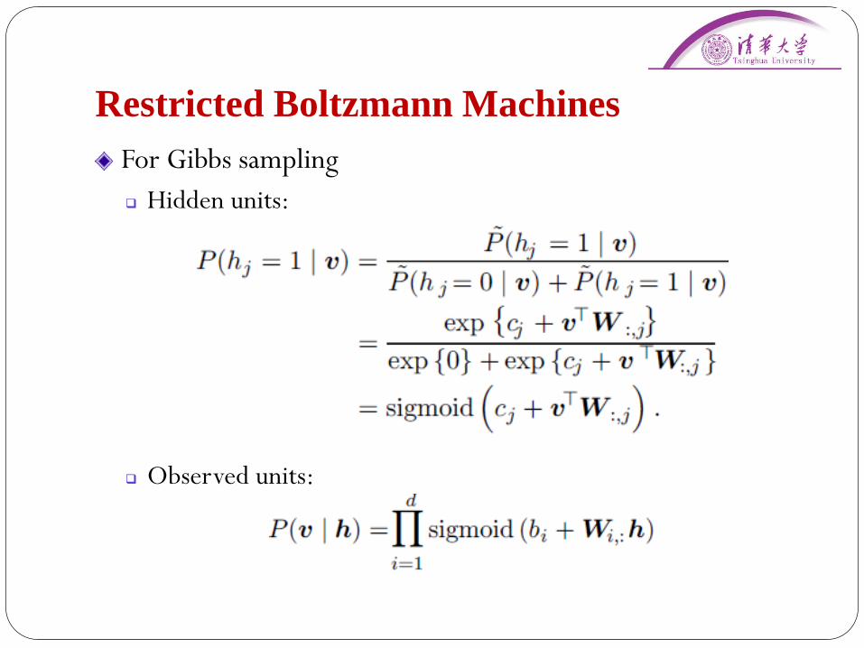
Restricted Boltzmann Machines
An energy-based model with hidden units
Graphical structure:
Restrict the connectivity to make learning easier.

Restricted Boltzmann Machines
Factorized conditional distribution over hidden units
Restricted Boltzmann Machines
For Gibbs sampling
Hidden units:
Observed units:

MLE
Log-likelihood
Gradient

Contrastive Divergence (CD)
Gibbs sampling for negative phase
Random initialization: v’->h’-
> … -> v -> h
Slow because of long burn-in
period
Intuition of CD
Start from a data closed to the
model samples
CD-k for negative phase
Start from empirical data and ran
k-steps
Typically, k=1: v1->h1->v2->h2

RBM
Filters
Samples (RBM is a generative model)

Issues with RBM
Log-partition function is intractable
No direct metric for choosing hyper-parameters
(one hidden layer) Much too simple for modeling high-
dimensional and richly structured sensory data

Deep Belief Nets – deep generative model
[Hinton et al., 2006]
Stacking RBM
Greedy layerwise training
Unsupervised learning
No labels
MLE
generationrecognition

Neural Evidence?
Our visual systems contain multilayer generative models
Top-down connections:
Generate low-level features of images from high-level
representations
Visual imagery, dreaming?
Bottom-up connections:
Infer the high-level representations that would have generated
an observed set of low-level features
[Hinton, Trends in Cognitive Science, 11(10), 2007]
Recent Advances on DGMsModels: Deep belief networks (Salakhutdinov & Hinton, 2009) Autoregressive models (Larochelle & Murray, 2011; Gregor et al., 2014) Stochastic variations of neural networks (Bengio et al., 2014) …
Applications: Image recognition (Ranzato et al., 2011) Inference of hidden object parts (Lee et al., 2009) Semi-supervised learning (Kingma et al., 2014) Multimodal learning (Srivastava & Salakhutdinov, 2014; Karpathy et al.,
2014) …
Learning algorithms Stochastic variational inference (Kingma & Welling, 2014; Rezende et al.,
2014) …

Learning with a Recognition Model
Characterize the variational distribution with a recognition model
For example:
where both mean and variance are nonlinear function of data by a DNN
x n
z n
N
y n
q Á ( z n )

Long Short-Term Memory
A RNN architecture without gradient vanishing issue
A RNN with LSTM blocks
Each block is a “smart” network, determing when to remember,
when to continue to remember or forget, and when to output
[Graves et al., 2009. A Novel Connectionist System for Improved Unconstrained Handwriting Recognition]

Issues
The sharpness of Gates’ activation functions maters!
[Lv & Zhu, 2014. Revisit Long Short-Term Memory: an Optimization Perspective]

Discussions

Challenges of DL
Learning
Backpropagation is slow and prone to gradient vanishing
Issues with non-convex optimization in high-dimensions
Overfitting
Big models are lacking of statistical information to fit
Interpretation
Deep nets are often used as black-box tools for learning and
inference
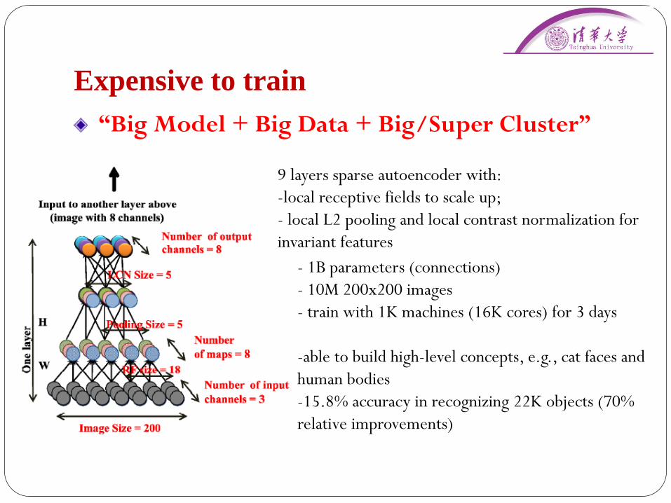
Expensive to train
9 layers sparse autoencoder with:
-local receptive fields to scale up;
- local L2 pooling and local contrast normalization for
invariant features
- 1B parameters (connections)
- 10M 200x200 images
- train with 1K machines (16K cores) for 3 days
-able to build high-level concepts, e.g., cat faces and
human bodies
-15.8% accuracy in recognizing 22K objects (70%
relative improvements)
“Big Model + Big Data + Big/Super Cluster”
Local Optima vs Saddle Points
Statistic Physics provide analytical tools
High-dimensional optimization problem
Most critical points are saddle points
The likelihood grows exponentially!

Dynamics of Various Opt. TechniquesSGD: Gradient is accurate, but may suffer from slow steps
Newton method: Wrong directions when negative curvatures present Saddle points become attractors! (can’t escape)
Saddle-free method: A generalization of Newton’s method to escape saddle points (more rapidly
than SGD)

Some Empirical Results

Overfitting in Big Data
Predictive information grows slower than the amount of
Shannon entropy (Bialek et al., 2001)

Overfitting in Big Data
Predictive information grows slower than the amount of
Shannon entropy (Bialek et al., 2001)
Model capacity grows faster than the amount of
predictive information!

Overfitting in DL
Increasing research attention, e.g., dropout training (Hinton,
2012)
More theoretical understanding and extensions
MCF (van der Maaten et al., 2013); Logistic-loss (Wager et al.,
2013); Dropout SVM (Chen, Zhu et al., 2014)

Model Complexity
What do we mean by structure learning in deep GMs? # of layers # of hidden units at each layer The type of each hidden unit (discrete
or continuous?) The connection structures (i.e., edges)
between hidden units
Adams et al. presented a structure learning method using nonparametric Bayesian techniques –a cascading IBP (CIBP) process [Admas, Wallach & Ghahramani, 2010]

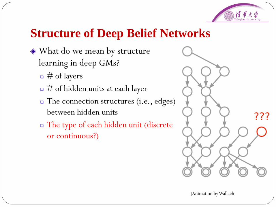
Structure of Deep Belief Networks
What do we mean by structure
learning in deep GMs?
# of layers
# of hidden units at each layer
The type of each hidden unit (discrete
or continuous?)
The connection structures (i.e., edges)
between hidden units
[Animation by Wallach]

Structure of Deep Belief Networks
What do we mean by structure
learning in deep GMs?
# of hidden units at each layer
# of layers
The type of each hidden unit (discrete
or continuous?)
The connection structures (i.e., edges)
between hidden units
[Animation by Wallach]

Structure of Deep Belief Networks
What do we mean by structure
learning in deep GMs?
# of hidden units at each layer
# of layers
The type of each hidden unit (discrete
or continuous?)
The connection structures (i.e., edges)
between hidden units
[Animation by Wallach]

Structure of Deep Belief Networks
What do we mean by structure
learning in deep GMs?
# of layers
# of hidden units at each layer
The connection structures (i.e., edges)
between hidden units
The type of each hidden unit (discrete
or continuous?)
[Animation by Wallach]
Structure of Deep Belief Networks
What do we mean by structure
learning in deep GMs?
# of layers
# of hidden units at each layer
The connection structures (i.e., edges)
between hidden units
The type of each hidden unit (discrete
or continuous?)
[Animation by Wallach]
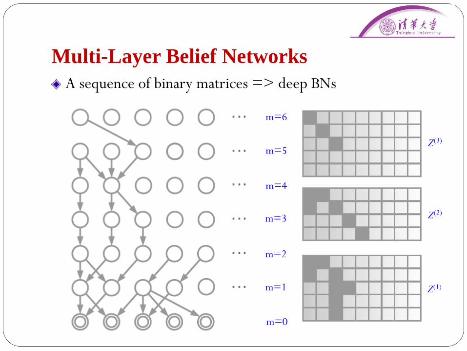
Multi-Layer Belief Networks
A sequence of binary matrices => deep BNs
m=0
m=1
m=2
m=3
m=4
m=5
m=6
Z(1)
Z(2)
Z(3)

The Cascading IBP (CIBP)
A stochastic process which results in an infinite sequence of
infinite binary matrices
Each matrix is exchangeable in both rows and columns
How do we know the CIBP converges?
The number of dishes in one layer depends only on the number
of customers in the previous layer
Can prove that this Markov chain reaches an absorbing state in
finite time with probability one

Samples from CIBP Prior
* only connected units are shown

Some counter-intuitive properties
Stability w.r.t small perturbations to inputs
Imperceptible non-random perturbation can arbitrarily change
the prediction (adversarial examples exist!)
[Szegedy et al., Intriguing properties of neural nets, 2013]
10x of
differences

Criticisms of DL
Just a buzzword, or largely a rebranding of neural networks
Lack of theory
gradient descent has been understood for a while
DL is often used as black-box
DL is only part of the larger challenge of building intelligent machines, still lacking of:
causal relationships
logic inferences
integrating abstract knowledge

How can neural science help?
The current DL models:
loosely inspired by the densely interconnected neurons of the brain
mimic human learning by changing weights based on experience
How to improve?
Transparent architecture? Attention mechanism?
Cheap learning? (partially) replace back-propagation?
Others?
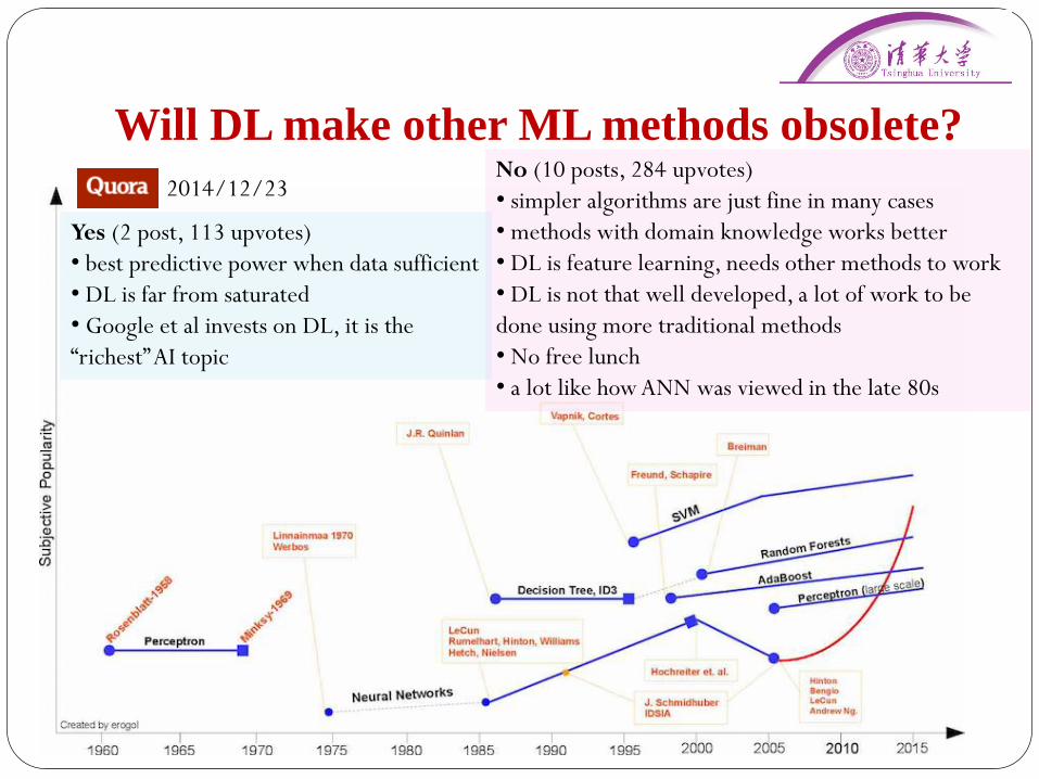
Will DL make other ML methods obsolete?
Yes (2 post, 113 upvotes)
• best predictive power when data sufficient
• DL is far from saturated
• Google et al invests on DL, it is the
“richest” AI topic
No (10 posts, 284 upvotes)
• simpler algorithms are just fine in many cases
• methods with domain knowledge works better
• DL is feature learning, needs other methods to work
• DL is not that well developed, a lot of work to be
done using more traditional methods
• No free lunch
• a lot like how ANN was viewed in the late 80s
2014/12/23

What are people saying?
Yann LeCun: “AI has gone from failure to failure, with bits of progress. This could
be another leapfrog”
Jitendra Malik: in the long term, deep learning may not win the day; … “Over time
people will decide what works best in different domains.” “Neural nets were always a delicate art to manage. There is some
black magic involved”
Andrew Ng: “Deep learning happens to have the property that if you feed it more
data it gets better and better,” “Deep-learning algorithms aren't the only ones like that, but they're
arguably the best — certainly the easiest. That's why it has huge promise for the future.”
[Nature 505, 146–148 (09 January 2014) ]

What are people saying?
Oren Etzioni:
“It‘s like when we invented flight” (not using the brain for
inspiration)
Alternatives:
Logic, knowledge base, grammars?
Quantum AI/ML?
[Nature 505, 146–148 (09 January 2014) ]

Thank You!