inferences about population variances - cengage · 2014-05-30 · inferences about population...
TRANSCRIPT

Inferences AboutPopulation Variances
CONTENTS
STATISTICS IN PRACTICE: U.S. GENERAL ACCOUNTABILITYOFFICE
11.1 INFERENCES ABOUT APOPULATION VARIANCEInterval EstimationUsing Excel to Construct a
Confidence Interval
Hypothesis TestingUsing Excel to Conduct a
Hypothesis Test
11.2 INFERENCES ABOUT TWOPOPULATION VARIANCESUsing Excel to Conduct a
Hypothesis Test
CHAPTER 11
56130_11_ch11_p449-475.qxd 2/22/08 11:03 PM Page 449
Cengage Learning

450 Chapter 11 Inferences About Population Variances
U.S. GENERAL ACCOUNTABILITY OFFICE*WASHINGTON, D.C.
STATISTICS in PRACTICE
The U.S. General Accountability Office (GAO) is anindependent, nonpolitical audit organization in the leg-islative branch of the federal government. GAO evalua-tors determine the effectiveness of current and proposedfederal programs. To carry out their duties, evaluatorsmust be proficient in records review, legislative research,and statistical analysis techniques.
In one case, GAO evaluators studied a Departmentof Interior program established to help clean up the na-tion’s rivers and lakes. As part of this program, federalgrants were made to small cities throughout the UnitedStates. Congress asked the GAO to determine how ef-fectively the program was operating. To do so, the GAO
examined records and visited the sites of several wastetreatment plants.
One objective of the GAO audit was to ensure that theeffluent (treated sewage) at the plants met certain stan-dards. Among other things the audits reviewed sampledata on the oxygen content, the pH level, and the amountof suspended solids in the effluent. A requirement of theprogram was that a variety of tests be taken daily at eachplant and that the collected data be sent periodically to thestate engineering department. The GAO’s investigationof the data showed whether various characteristics of theeffluent were within acceptable limits.
For example, the mean or average pH level of the ef-fluent was examined carefully. In addition, the variancein the reported pH levels was reviewed. The followinghypothesis test was conducted about the variance in pHlevel for the population of effluent.
In this test, is the population variance in pH level ex-pected at a properly functioning plant. In one particular
σ 20
H0:
Ha: σ 2 � σ 2
0
σ 2 � σ 20
plant, the null hypothesis was rejected. Further analysisshowed that this plant had a variance in pH level thatwas significantly less than normal.
The auditors visited the plant to examine the measur-ing equipment and to discuss their statistical findings withthe plant manager. The auditors found that the measuringequipment was not being used because the operator didnot know how to work it. Instead, the operator had beentold by an engineer what level of pH was acceptable andhad simply recorded similar values without actually con-ducting the test. The unusually low variance in this plant’sdata resulted in rejection of H0. The GAO suspected thatother plants might have similar problems and recom-mended an operator training program to improve the datacollection aspect of the pollution control program.
In this chapter you will learn how to conduct statisti-cal inferences about the variances of one and two popu-lations. Two new probability distributions, the chi-squaredistribution and the F distribution, will be introducedand used to make interval estimates and hypothesis testsabout population variances.
Effluent at this facility must fall within a statisticallydetermined pH range. © Jason Hawkes/WorkbookStock/Jupiter Images
In the preceding four chapters we examined methods of statistical inference involving population means and population proportions. In this chapter we expand the discussion tosituations involving inferences about population variances. As an example of a case inwhich a variance can provide important decision-making information, consider the pro-duction process of filling containers with a liquid detergent product. The filling mechanismfor the process is adjusted so that the mean filling weight is 16 ounces per container.
*The authors thank Art Foreman and Dale Ledman of the U.S. GeneralAccountability Office for providing this Statistics in Practice.
56130_11_ch11_p449-475.qxd 2/22/08 11:03 PM Page 450
Cengage Learning
11.1 Inferences About a Population Variance 451
Although a mean of 16 ounces is desired, the variance of the filling weights is also critical.That is, even with the filling mechanism properly adjusted for the mean of 16 ounces, wecannot expect every container to have exactly 16 ounces. By selecting a sample of con-tainers, we can compute a sample variance for the number of ounces placed in a container.This value will serve as an estimate of the variance for the population of containers beingfilled by the production process. If the sample variance is small, the production process willbe continued. However, if the sample variance is excessive, overfilling and underfilling maybe occurring even though the mean is correct at 16 ounces. In this case, the filling mecha-nism will be readjusted in an attempt to reduce the filling variance for the containers.
In the first section we consider inferences about the variance of a single population.Subsequently, we will discuss procedures that can be used to make inferences about thevariances of two populations.
11.1 Inferences About a Population VarianceThe sample variance
(11.1)
is the point estimator of the population variance σ 2. In using the sample variance as a basisfor making inferences about a population variance, the sampling distribution of the quan-tity (n � 1)s2/σ 2 is helpful. This sampling distribution is described as follows.
s2 ��(xi � x̄)2
n � 1
In many manufacturingapplications, controllingthe process variance isextremely important inmaintaining quality.
SAMPLING DISTRIBUTION OF (n � 1)s2/σ 2
Whenever a simple random sample of size n is selected from a normal population, thesampling distribution of
(11.2)
has a chi-square distribution with n � 1 degrees of freedom.
(n � 1)s2
σ 2
The chi-square distributionis based on sampling froma normal population.
Figure 11.1 shows some possible forms of the sampling distribution of (n � 1)s2/σ 2.Tables of areas or probabilities are readily available for the chi-square distribution.
Since the sampling distribution of (n � 1)s2/σ 2 is known to have a chi-square distributionwhenever a simple random sample of size n is selected from a normal population, we canuse the chi-square distribution to develop interval estimates and conduct hypothesis testsabout a population variance.
Interval EstimationTo show how the chi-square distribution can be used to develop a confidence intervalestimate of a population variance σ 2, suppose that we are interested in estimating thepopulation variance for the container filling process mentioned in the chapter introduction.A sample of 20 containers is taken, and the sample variance for the filling weights is foundto be s2 � .0025. We know we cannot expect the variance of a sample of 20 containers toprovide the exact value of the variance for the population of containers filled by the pro-duction process. Hence, our interest will be in developing an interval estimate for the popu-lation variance.
Excel’s CHIDIST functioncan be used to computeprobabilities for the chi-square distribution.
fileCDDetergent
56130_11_ch11_p449-475.qxd 2/22/08 11:03 PM Page 451
Cengage Learning

452 Chapter 11 Inferences About Population Variances
With 2 degrees of freedom
With 5 degrees of freedom
With 10 degrees of freedom
σ 2(n – 1)s2
0
FIGURE 11.1 EXAMPLES OF THE SAMPLING DISTRIBUTION OF (n � 1)s2/σ 2
(A CHI-SQUARE DISTRIBUTION)
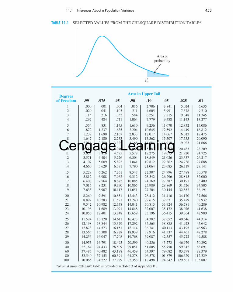
We will use the notation to denote the value for the chi-square distribution that provides an area or probability of α to the right of the value. For example, in Figure 11.2the chi-square distribution with 19 degrees of freedom is shown with � 32.852indicating that 2.5% of the chi-square values are to the right of 32.852, and � 8.907indicating that 97.5% of the chi-square values are to the right of 8.907. Refer to Table 11.1and verify that these chi-square values with 19 degrees of freedom (19th row of thetable) are correct. Table 3 of Appendix B provides a more extensive table of chi-squarevalues.
From the graph in Figure 11.2 we see that .95, or 95%, of the chi-square values arebetween and . That is, there is a .95 probability of obtaining a � 2 value such that
�2.975 � �2 � �2
.025
� 2.025� 2
.975
� 2.975
� 2.025
� 2α
� 2α
0 8.907 32.852
.025.025
.95 of thepossible valuesχ2
χ 2
χ 2.025χ 2
.975
FIGURE 11.2 A CHI-SQUARE DISTRIBUTION WITH 19 DEGREES OF FREEDOM
56130_11_ch11_p449-475.qxd 2/22/08 11:03 PM Page 452
Cengage Learning
11.1 Inferences About a Population Variance 453
DegreesArea in Upper Tail
of Freedom .99 .975 .95 .90 .10 .05 .025 .011 .000 .001 .004 .016 2.706 3.841 5.024 6.6352 .020 .051 .103 .211 4.605 5.991 7.378 9.2103 .115 .216 .352 .584 6.251 7.815 9.348 11.3454 .297 .484 .711 1.064 7.779 9.488 11.143 13.277
5 .554 .831 1.145 1.610 9.236 11.070 12.832 15.0866 .872 1.237 1.635 2.204 10.645 12.592 14.449 16.8127 1.239 1.690 2.167 2.833 12.017 14.067 16.013 18.4758 1.647 2.180 2.733 3.490 13.362 15.507 17.535 20.0909 2.088 2.700 3.325 4.168 14.684 16.919 19.023 21.666
10 2.558 3.247 3.940 4.865 15.987 18.307 20.483 23.20911 3.053 3.816 4.575 5.578 17.275 19.675 21.920 24.72512 3.571 4.404 5.226 6.304 18.549 21.026 23.337 26.21713 4.107 5.009 5.892 7.041 19.812 22.362 24.736 27.68814 4.660 5.629 6.571 7.790 21.064 23.685 26.119 29.141
15 5.229 6.262 7.261 8.547 22.307 24.996 27.488 30.57816 5.812 6.908 7.962 9.312 23.542 26.296 28.845 32.00017 6.408 7.564 8.672 10.085 24.769 27.587 30.191 33.40918 7.015 8.231 9.390 10.865 25.989 28.869 31.526 34.80519 7.633 8.907 10.117 11.651 27.204 30.144 32.852 36.191
20 8.260 9.591 10.851 12.443 28.412 31.410 34.170 37.56621 8.897 10.283 11.591 13.240 29.615 32.671 35.479 38.93222 9.542 10.982 12.338 14.041 30.813 33.924 36.781 40.28923 10.196 11.689 13.091 14.848 32.007 35.172 38.076 41.63824 10.856 12.401 13.848 15.659 33.196 36.415 39.364 42.980
25 11.524 13.120 14.611 16.473 34.382 37.652 40.646 44.31426 12.198 13.844 15.379 17.292 35.563 38.885 41.923 45.64227 12.878 14.573 16.151 18.114 36.741 40.113 43.195 46.96328 13.565 15.308 16.928 18.939 37.916 41.337 44.461 48.27829 14.256 16.047 17.708 19.768 39.087 42.557 45.722 49.588
30 14.953 16.791 18.493 20.599 40.256 43.773 46.979 50.89240 22.164 24.433 26.509 29.051 51.805 55.758 59.342 63.69160 37.485 40.482 43.188 46.459 74.397 79.082 83.298 88.37980 53.540 57.153 60.391 64.278 96.578 101.879 106.629 112.329
100 70.065 74.222 77.929 82.358 118.498 124.342 129.561 135.807
*Note: A more extensive table is provided as Table 3 of Appendix B.
TABLE 11.1 SELECTED VALUES FROM THE CHI-SQUARE DISTRIBUTION TABLE*
Area orprobability
χ 2α
56130_11_ch11_p449-475.qxd 2/22/08 11:03 PM Page 453
Cengage Learning

454 Chapter 11 Inferences About Population Variances
We stated in expression (11.2) that (n � 1)s2/σ 2 follows a chi-square distribution; therefore,we can substitute (n � 1)s2/σ 2 for � 2 and write
(11.3)
In effect, expression (11.3) provides an interval estimate in that .95, or 95%, of all possiblevalues for (n � 1)s2/σ 2 will be in the interval to . We now need to do some alge-braic manipulations with expression (11.3) to develop an interval estimate for the popula-tion variance σ 2. Working with the leftmost inequality in expression (11.3), we have
Thus
or
(11.4)
Performing similar algebraic manipulations with the rightmost inequality in expression (11.3)gives
(11.5)
The results of expressions (11.4) and (11.5) can be combined to provide
(11.6)
Because expression (11.3) is true for 95% of the (n � 1)s2/σ 2 values, expression (11.6)provides a 95% confidence interval estimate for the population variance σ 2.
Let us return to the problem of providing an interval estimate for the population vari-ance of filling weights. Recall that the sample of 20 containers provided a sample variance ofs2 � .0025. With a sample size of 20, we have 19 degrees of freedom.As shown in Figure 11.2,we have already determined that � 8.907 and � 32.852. Using these values inexpression (11.6) provides the following interval estimate for the population variance.
or
Taking the square root of these values provides the following 95% confidence interval forthe population standard deviation.
.0380 � σ � .0730
.001446 � σ 2 � .005333
(19)(.0025)
32.852� σ 2 �
(19)(.0025)
8.907
� 2.025� 2
.975
(n � 1)s2
� 2.025
� σ 2 �(n � 1)s2
� 2.975
(n � 1)s2
� 2.025
� σ 2
σ 2 �(n � 1)s2
� 2.975
σ 2� 2.975 � (n � 1)s2
� 2.975 �
(n � 1)s2
σ 2
� 2.025� 2
.975
� 2.975 �
(n � 1)s2
σ 2 � � 2.025
A confidence interval for apopulation standarddeviation can be found bycomputing the square rootsof the lower limit and upperlimit of the confidenceinterval for the populationvariance.
56130_11_ch11_p449-475.qxd 2/22/08 11:03 PM Page 454
Cengage Learning

A B C D E1 Ounces Interval Estimate of a Population Variance2 15.923 16.02 Sample Size =COUNT(A2:A21)4 15.99 Variance =VAR(A2:A21)5 16.026 15.91 Confidence Coefficient 0.957 15.98 Level of Significance =1-D68 16.06 Chi-Square Value (lower tail) =CHIINV(1-D7/2,D3-1)9 15.97 Chi-Square Value (upper tail) =CHIINV(D7/2,D3-1)
10 15.9711 16.07 Point Estimate =D412 15.94 Lower Limit =((D3-1)*D4)/D913 15.96 Upper Limit =((D3-1)*D4)/D814 16.0415 16.0116 16.0717 16.0118 15.919 15.9620 1621 15.9922
11.1 Inferences About a Population Variance 455
Thus, we illustrated the process of using the chi-square distribution to establish interval es-timates of a population variance and a population standard deviation. Note specifically thatbecause and were used, the interval estimate has a .95 confidence coefficient. Ex-tending expression (11.6) to the general case of any confidence coefficient, we have the fol-lowing interval estimate of a population variance.
� 2.025� 2
.975
INTERVAL ESTIMATE OF A POPULATION VARIANCE
(11.7)
where the � 2 values are based on a chi-square distribution with n � 1 degrees of free-dom and where 1 � α is the confidence coefficient.
(n � 1)s2
� 2α/2
� σ 2 �(n � 1)s2
� 2(1�α/2)
FIGURE 11.3 EXCEL WORKSHEET FOR THE LIQUID DETERGENT FILLING PROCESS
A B C D E1 Ounces Interval Estimate of a Population Variance2 15.923 16.02 Sample Size 204 15.99 Variance 0.00255 16.026 15.91 Confidence Coefficient 0.957 15.98 Level of Significance 0.058 16.06 Chi-Square Value (lower tail) 8.90659 15.97 Chi-Square Value (upper tail) 32.8523
10 15.9711 16.07 Point Estimate 0.002512 15.94 Lower Limit 0.001413 15.96 Upper Limit 0.005314 16.0415 16.0116 16.0717 16.0118 15.9019 15.9620 16.0021 15.9922
fileCDDetergent
Using Excel to Construct a Confidence IntervalExcel can be used to construct a 95% confidence interval of the population variance for theexample involving filling containers with a liquid detergent product. Refer to Figure 11.3as we describe the tasks involved. The formula worksheet is in the background; the valueworksheet is in the foreground.
Enter Data: Column A shows the number of ounces of detergent for each of the 20containers.
Enter Functions and Formulas: The descriptive statistics needed are provided in cellsD3:D4. Excel’s COUNT and VAR functions are used to compute the sample size and thesample variance, respectively.
56130_11_ch11_p449-475.qxd 2/22/08 11:03 PM Page 455
Cengage Learning
Cells D6:D9 are used to compute the appropriate chi-square values. The confidence co-efficient was entered into cell D6 and the level of significance (α) was computed in cell D7by entering the formula �1-D6. Excel’s CHIINV function was used to compute the lower-and upper-tail chi-square values. The form of the CHIINV function is CHIINV(upper-tailprobability, degrees of freedom). The formula �CHIINV(1-D7/2,D3-1) was entered into cellD8 to compute the chi-square value in the lower tail. The value worksheet shows that the chi-square value for 19 degrees of freedom is � 8.9065. Then, to compute the chi-squarevalue corresponding to an upper-tail probability of .025, the function �CHIINV(D7/2,D3-1)was entered into cell D9. The value worksheet shows that the chi-square value obtained is
� 32.8523.Cells D11:D13 provide the point estimate and the lower and upper limits for the confidence
interval. Because the point estimate is just the sample variance, we entered the formula �D4into cell D11. Inequality (11.7) shows that the lower limit of the 95% confidence interval is
Thus, to compute the lower limit of the 95% confidence interval, the formula �((D3-1)*D4)/D9 was entered into cell D12. Inequality (11.7) also shows that the upper limit ofthe confidence interval is
Thus, to compute the upper limit of the 95% confidence interval, the formula �((D3-1)*D4)/D8was entered into cell D13. The value worksheet shows a lower limit of .0014 and an upperlimit of .0053. In other words, the 95% confidence interval estimate of the populationvariance is from .0014 to .0053.
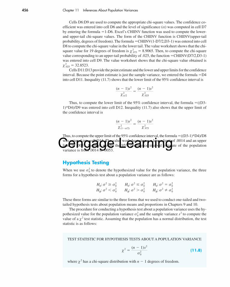
Hypothesis TestingWhen we use to denote the hypothesized value for the population variance, the threeforms for a hypothesis test about a population variance are as follows:
These three forms are similar to the three forms that we used to conduct one-tailed and two-tailed hypothesis tests about population means and proportions in Chapters 9 and 10.
The procedure for conducting a hypothesis test about a population variance uses the hy-pothesized value for the population variance and the sample variance s2 to compute thevalue of a � 2 test statistic. Assuming that the population has a normal distribution, the teststatistic is as follows:
σ 20
H0:
Ha: σ 2 � σ 2
0
σ 2 � σ 20
H0:
Ha: σ 2 � σ 2
0
σ 2 � σ 20
H0:
Ha: σ 2 � σ 2
0
σ 2 � σ 20
σ 20
(n � 1)s2
� 2(1�α/2)
�(n � 1)s2
� 2.975
(n � 1)s2
� 2α/2
�(n � 1)s2
� 2.025
� 2.025
� 2.975
456 Chapter 11 Inferences About Population Variances
TEST STATISTIC FOR HYPOTHESIS TESTS ABOUT A POPULATION VARIANCE
(11.8)
where � 2 has a chi-square distribution with n � 1 degrees of freedom.
� 2 �(n � 1)s2
σ 20
56130_11_ch11_p449-475.qxd 2/22/08 11:03 PM Page 456
Cengage Learning
After computing the value of the � 2 test statistic, either the p-value approach or the criticalvalue approach may be used to determine whether the null hypothesis can be rejected.
Let us consider the following example. The St. Louis Metro Bus Company wants topromote an image of reliability by encouraging its drivers to maintain consistent schedules.As a standard policy the company would like arrival times at bus stops to have low vari-ability. In terms of the variance of arrival times, the company standard specifies an arrivaltime variance of 4 or less when arrival times are measured in minutes. The following hy-pothesis test is formulated to help the company determine whether the arrival time popula-tion variance is excessive.
In tentatively assuming H0 is true, we are assuming that the population variance of ar-rival times is within the company guideline. We reject H0 if the sample evidence indicatesthat the population variance exceeds the guideline. In this case, follow-up steps should betaken to reduce the population variance. We will conduct the hypothesis test using a levelof significance of α � .05.
Suppose that a random sample of 24 bus arrivals taken at a downtown intersection pro-vides a sample variance of s2 � 4.9. Assuming that the population distribution of arrivaltimes is approximately normal, the value of the test statistic is as follows:
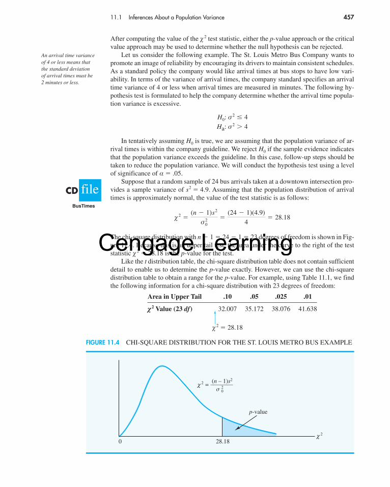
The chi-square distribution with n � 1 � 24 � 1 � 23 degrees of freedom is shown in Fig-ure 11.4. Because this is an upper tail test, the area under the curve to the right of the teststatistic � 2 � 28.18 is the p-value for the test.
Like the t distribution table, the chi-square distribution table does not contain sufficientdetail to enable us to determine the p-value exactly. However, we can use the chi-squaredistribution table to obtain a range for the p-value. For example, using Table 11.1, we findthe following information for a chi-square distribution with 23 degrees of freedom:
� 2 �(n � 1)s2
σ 20
�(24 � 1)(4.9)
4� 28.18
H0:
Ha: σ 2 � 4
σ 2 � 4
11.1 Inferences About a Population Variance 457
An arrival time variance of 4 or less means that the standard deviation of arrival times must be 2 minutes or less.
Area in Upper Tail .10 .05 .025 .01
� 2 Value (23 df) 32.007 35.172 38.076 41.638
� 2 � 28.18
fileCDBusTimes
0 28.18
p-value
χ 2
=(n – 1)
2σ χ 2
0
s2
FIGURE 11.4 CHI-SQUARE DISTRIBUTION FOR THE ST. LOUIS METRO BUS EXAMPLE
56130_11_ch11_p449-475.qxd 2/22/08 11:03 PM Page 457
Cengage Learning

458 Chapter 11 Inferences About Population Variances
Area in Upper Tail .10 .05 .025 .01
� 2 Value (29 df) 39.087 42.557 45.722 49.588
� 2 � 46.98
Because � 2 � 28.18 is less than 32.007, the area in the upper tail (the p-value) is greaterthan .10. Excel can be used to show that � 2 � 28.18 provides a p-value � .2091. With thep-value � α � .05, we cannot reject the null hypothesis. The sample does not support theconclusion that the population variance of the arrival times is excessive.
As with other hypothesis testing procedures, the critical value approach can also be usedto draw the hypothesis testing conclusion. With α � .05, provides the critical value forthe upper tail hypothesis test. Using Table 11.1 and 23 degrees of freedom, � 35.172.Thus, the rejection rule for the bus arrival time example is as follows:
Because the value of the test statistic is � 2 � 28.18, we cannot reject the null hypothesis.In practice, upper tail tests as presented here are the most frequently encountered tests
about a population variance. In situations involving arrival times, production times, fillingweights, part dimensions, and so on, low variances are desirable, whereas large variancesare unacceptable. With a statement about the maximum allowable population variance, wecan test the null hypothesis that the population variance is less than or equal to the maxi-mum allowable value against the alternative hypothesis that the population variance isgreater than the maximum allowable value. With this test structure, corrective action willbe taken whenever rejection of the null hypothesis indicates the presence of an excessivepopulation variance.
As we saw with population means and proportions, other forms of hypothesis tests canbe developed. Let us demonstrate a two-tailed test about a population variance by consid-ering a situation faced by a bureau of motor vehicles. Historically, the variance in test scoresfor individuals applying for driver’s licenses has been σ 2 � 100. A new examination withnew test questions has been developed. Administrators of the bureau of motor vehicleswould like the variance in the test scores for the new examination to remain at the histori-cal level. To evaluate the variance in the new examination test scores, the following two-tailed hypothesis test has been proposed:
Rejection of H0 will indicate that a change in the variance has occurred and suggest thatsome questions in the new examination may need revision to make the variance of the new test scores similar to the variance of the old test scores. A sample of 30 applicants fordriver’s licenses will be given the new version of the examination. We will use a level ofsignificance α � .05 to conduct the hypothesis test.
The sample of 30 examination scores provided a sample variance s2 � 162. The valueof the chi-square test statistic is as follows:
Now, let us compute the p-value. Using Table 11.1 and n � 1 � 30 � 1 � 29 degrees offreedom, we find the following:
� 2 �(n � 1)s2
σ 20
�(30 � 1)(162)
100� 46.98
H0:
Ha: σ 2 � 100
σ 2 � 100
Reject H0 if �2 � 35.172
� 2.05
� 2.05
Using Excel, p-value �
CHIDIST (28.18,23) �
.2091.
56130_11_ch11_p449-475.qxd 2/22/08 11:03 PM Page 458
Cengage Learning
11.1 Inferences About a Population Variance 459
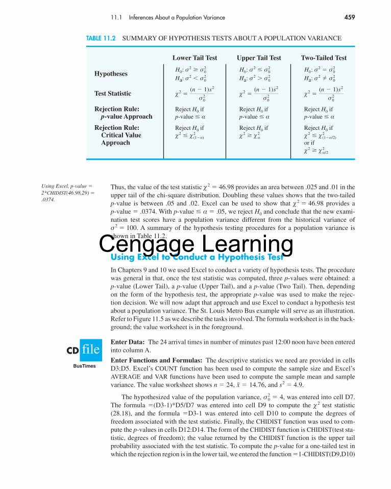
Thus, the value of the test statistic � 2 � 46.98 provides an area between .025 and .01 in theupper tail of the chi-square distribution. Doubling these values shows that the two-tailed p-value is between .05 and .02. Excel can be used to show that � 2 � 46.98 provides a p-value � .0374. With p-value � α � .05, we reject H0 and conclude that the new exami-nation test scores have a population variance different from the historical variance ofσ 2 � 100. A summary of the hypothesis testing procedures for a population variance isshown in Table 11.2.
Using Excel to Conduct a Hypothesis TestIn Chapters 9 and 10 we used Excel to conduct a variety of hypothesis tests. The procedurewas general in that, once the test statistic was computed, three p-values were obtained: a p-value (Lower Tail), a p-value (Upper Tail), and a p-value (Two Tail). Then, depending on the form of the hypothesis test, the appropriate p-value was used to make the rejec-tion decision. We will now adapt that approach and use Excel to conduct a hypothesis testabout a population variance. The St. Louis Metro Bus example will serve as an illustration.Refer to Figure 11.5 as we describe the tasks involved. The formula worksheet is in the back-ground; the value worksheet is in the foreground.
Enter Data: The 24 arrival times in number of minutes past 12:00 noon have been enteredinto column A.
Enter Functions and Formulas: The descriptive statistics we need are provided in cellsD3:D5. Excel’s COUNT function has been used to compute the sample size and Excel’sAVERAGE and VAR functions have been used to compute the sample mean and samplevariance. The value worksheet shows n � 24, and s2 � 4.9.
The hypothesized value of the population variance, was entered into cell D7.The formula �(D3-1)*D5/D7 was entered into cell D9 to compute the � 2 test statistic(28.18), and the formula �D3-1 was entered into cell D10 to compute the degrees offreedom associated with the test statistic. Finally, the CHIDIST function was used to com-pute the p-values in cells D12:D14. The form of the CHIDIST function is CHIDIST(test sta-tistic, degrees of freedom); the value returned by the CHIDIST function is the upper tailprobability associated with the test statistic. To compute the p-value for a one-tailed test inwhich the rejection region is in the lower tail, we entered the function �1-CHIDIST(D9,D10)
σ 20 � 4,
x̄ � 14.76,
Using Excel, p-value �
2*CHIDIST(46.98,29) �
.0374.
Lower Tail Test Upper Tail Test Two-Tailed Test
Hypotheses
Test Statistic
Rejection Rule: Reject H0 if Reject H0 if Reject H0 ifp-value Approach p-value � α p-value � α p-value � α
Rejection Rule: Reject H0 if Reject H0 if Reject H0 ifCritical ValueApproach or if
� 2 � � 2α/2
� 2 � � 2(1�α/2)� 2 � � 2
α� 2 � � 2(1�α)
� 2 �(n � 1)s2
σ 20
� 2 �(n � 1)s2
σ 20
� 2 �(n � 1)s2
σ 20
H0:
Ha: σ 2 � σ 2
0
σ 2 � σ 20
H0:
Ha: σ 2 � σ 2
0
σ 2 � σ 20
H0:
Ha: σ 2 � σ 2
0
σ 2 � σ 20
TABLE 11.2 SUMMARY OF HYPOTHESIS TESTS ABOUT A POPULATION VARIANCE
fileCDBusTimes
56130_11_ch11_p449-475.qxd 2/22/08 11:03 PM Page 459
Cengage Learning

A B C D E1 Times Hypothesis Test About a Population Variance2 15.73 16.9 Sample Size =COUNT(A2:A25)4 12.8 Sample Mean =AVERAGE(A2:A25)5 15.6 Sample Variance =VAR(A2:A25)6 147 16.2 Hypothesized Value 48 14.89 19.8 Test Statistic =(D3-1)*D5/D7
10 13.2 Degrees of Freedom =D3-111 15.312 14.7 p-value (Lower Tail) =1-CHIDIST(D9,D10)13 10.2 p-value (Upper Tail) =CHIDIST(D9,D10)14 16.7 p-value (Two Tail) =2*MIN(D12,D13)15 13.625 12.726
460 Chapter 11 Inferences About Population Variances
into cell D12. Similarly, to compute the p-value for a one-tailed test in which the rejection re-gion is in the upper tail, we entered the function �CHIDIST(D9,D10) into cell D13. Finally,to compute the p-value for a two-tailed test, we entered the function �2*MIN(D12,D13)into cell D14. The value worksheet shows that p-value (Lower Tail) � .7909, p-value (Up-per Tail) � .2091, and p-value (Two Tail) � .4181. The rejection region for the St. LouisMetro Bus example is in the upper tail; thus, the appropriate p-value is .2091. At a .05 levelof significance, we cannot reject H0 because .2091 � .05. Hence, the sample variance ofs2 � 4.9 is insufficient evidence to conclude that the arrival time variance is not meeting thecompany standard.
This worksheet can be used as a template for other hypothesis tests about a populationvariance. Enter the data in column A, revise the ranges for the functions in cells D3:D5 asappropriate for the data, and type the hypothesized value in cell D7. The p-value appro-priate for the test can then be selected from cells D12:D14. The worksheet can also be usedfor exercises in which the sample size, sample variance, and hypothesized value are given.For instance, in the previous subsection we conducted a two-tailed hypothesis test about thevariance in scores on a new examination given by the bureau of motor vehicles. The sam-ple size was 30, the sample variance was s2 � 162, and the hypothesized value for the population variance was Using the worksheet in Figure 11.5, we can type 30into cell D3, 162 into cell D5, and 100 into cell D7. The correct two-tailed p-value will thenbe given in cell D14. Try it. You should get a p-value of .0374.
Exercises
Methods1. Find the following chi-square distribution values from Table 11.1 or Table 3 ofAppendix B.
a. with df � 5b. with df � 15� 2
.025
� 2.05
σ 20 � 100.
σ 20
To avoid having to revisethe cell ranges for functionsin cells D3:D5, the A:Amethod of specifying cellranges can be used.
FIGURE 11.5 HYPOTHESIS TEST FOR VARIANCE IN BUS ARRIVAL TIMES
A B C D E1 Times Hypothesis Test About a Population Variance2 15.73 16.9 Sample Size 244 12.8 Sample Mean 14.765 15.6 Sample Variance 4.96 14.07 16.2 Hypothesized Value 48 14.89 19.8 Test Statistic 28.18
10 13.2 Degrees of Freedom 2311 15.312 14.7 p-value (Lower Tail) 0.790913 10.2 p-value (Upper Tail) 0.209114 16.7 p-value (Two Tail) 0.418115 13.625 12.726
Note: Rows 16–24 are hidden.
56130_11_ch11_p449-475.qxd 2/22/08 11:03 PM Page 460
Cengage Learning

11.1 Inferences About a Population Variance 461
c. with df � 20d. with df � 10e. with df � 18
2. A sample of 20 items provides a sample standard deviation of 5.a. Compute the 90% confidence interval estimate of the population variance.b. Compute the 95% confidence interval estimate of the population variance.c. Compute the 95% confidence interval estimate of the population standard deviation.
3. A sample of 16 items provides a sample standard deviation of 9.5. Test the following hy-potheses using α � .05. What is your conclusion? Use both the p-value approach and thecritical value approach.
Applications4. The variance in drug weights is critical in the pharmaceutical industry. For a specific drug,
with weights measured in grams, a sample of 18 units provided a sample variance of s2 � .36.a. Construct a 90% confidence interval estimate of the population variance for the weight
of this drug.b. Construct a 90% confidence interval estimate of the population standard deviation.
5. The daily car rental rates for a sample of eight cities follow.
H0:
Ha: σ 2 � 50
σ 2 � 50
� 2.95
� 2.01
� 2.975
Daily Car Daily CarCity Rental Rate ($) City Rental Rate ($)
Atlanta 47 Phoenix 40Chicago 50 Pittsburgh 43Dallas 53 San Francisco 39New Orleans 45 Seattle 37
testSELF
a. Compute the variance and the standard deviation for these data.b. What is the 95% confidence interval estimate of the variance of car rental rates for the
population?c. What is the 95% confidence interval estimate of the standard deviation for the population?
6. The Fidelity Growth & Income mutual fund received a three-star, or neutral, rating fromMorningstar. Shown here are the quarterly percentage returns for the five-year period from2001 to 2005 (Morningstar Funds 500, 2006).
1st Quarter 2nd Quarter 3rd Quarter 4th Quarter
2001 �10.91 5.80 �9.64 6.452002 0.83 �10.48 �14.03 5.582003 �2.27 10.43 0.85 9.332004 1.34 1.11 �0.77 8.032005 �2.46 0.89 2.55 1.78
fileCDReturn
a. Compute the mean, variance, and standard deviation for the quarterly returns.b. Financial analysts often use standard deviation as a measure of risk for stocks and mu-
tual funds. Develop a 95% confidence interval for the population standard deviationof quarterly returns for the Fidelity Growth & Income mutual fund.
56130_11_ch11_p449-475.qxd 2/22/08 11:03 PM Page 461
Cengage Learning

462 Chapter 11 Inferences About Population Variances
7. To analyze the risk, or volatility, associated with investing in Chevron Corporation com-mon stock, a sample of the monthly total percentage return for 12 months was taken. Thereturns for the 12 months of 2005 are shown here (Compustat, February 24, 2006). Totalreturn is price appreciation plus any dividend paid.
testSELF
Month Return (%) Month Return (%)
January 3.60 July 3.74February 14.86 August 6.62March �6.07 September 5.42April �10.82 October �11.83May 4.29 November 1.21June 3.98 December �.94
a. Compute the sample variance and sample standard deviation as a measure of volatil-ity of monthly total return for Chevron.
b. Construct a 95% confidence interval for the population variance.c. Construct a 95% confidence interval for the population standard deviation.
8. A group of 12 security analysts provided estimates of the year 2001 earnings per share forQualcomm, Inc. (http://Zacks.com, June 13, 2000). The data are as follows:
1.40 1.40 1.45 1.49 1.37 1.27 1.40 1.55 1.40 1.42 1.48 1.63
a. Compute the sample variance for the earnings per share estimate.b. Compute the sample standard deviation for the earnings per share estimate.c. Provide 95% confidence interval estimates of the population variance and the popu-
lation standard deviation.
9. An automotive part must be machined to close tolerances to be acceptable to customers.Production specifications call for a maximum variance in the lengths of the parts of .0004.Suppose the sample variance for 30 parts turns out to be s2 � .0005. Using α � .05, testto see whether the population variance specification is being violated.
10. The average standard deviation for the annual return of large cap stock mutual funds is18.2% (The Top Mutual Funds, AAII, 2004). The sample standard deviation based on asample of size 36 for the Vanguard PRIMECAP mutual fund is 22.2%. Construct a hy-pothesis test that can be used to determine whether the standard deviation for the Vanguardfund is greater than the average standard deviation for large cap mutual funds. With a .05level of significance, what is your conclusion?
11. Home mortgage interest rates for 30-year fixed-rate loans vary throughout the country. Dur-ing the summer of 2000, data available from various parts of the country suggested that the standard deviation of the interest rates was .096 (The Wall Street Journal, Septem-ber 8, 2000). The corresponding variance in interest rates would be (.096)2 � .009216. Con-sider a follow-up study in the summer of 2005. The interest rates for 30-year fixed rate loansat a sample of 20 lending institutions had a sample standard deviation of .114. Conduct ahypothesis test using H0: σ
2 � .009216 to see whether the sample data indicate that the vari-ability in interest rates changed. Use α � .05. What is your conclusion?
12. A Fortune study found that the variance in the number of vehicles owned or leased by sub-scribers to Fortune magazine is .94. Assume a sample of 12 subscribers to another maga-zine provided the following data on the number of vehicles owned or leased: 2, 1, 2, 0, 3,2, 2, 1, 2, 1, 0, and 1.a. Compute the sample variance in the number of vehicles owned or leased by the 12
subscribers.b. Test the hypothesis H0: σ
2 � .94 to determine whether the variance in the number ofvehicles owned or leased by subscribers of the other magazine differs from σ 2 � .94for Fortune. At a .05 level of significance, what is your conclusion?
56130_11_ch11_p449-475.qxd 2/22/08 11:03 PM Page 462
Cengage Learning
11.2 Inferences About Two Population Variances 463
11.2 Inferences About Two Population VariancesIn some statistical applications we may want to compare the variances in product qualityresulting from two different production processes, the variances in assembly times for two assembly methods, or the variances in temperatures for two heating devices. In mak-ing comparisons about the two population variances, we will be using data collected fromtwo independent random samples, one from population 1 and another from population 2.The two sample variances and will be the basis for making inferences about the twopopulation variances and . Whenever the variances of two normal populations areequal ( ), the sampling distribution of the ratio of the two sample variances is as follows.
s21 �s2
2σ 21 � σ 2
2
σ 22σ 2
1
s22s2
1
0 2.12
.05
F.05
F
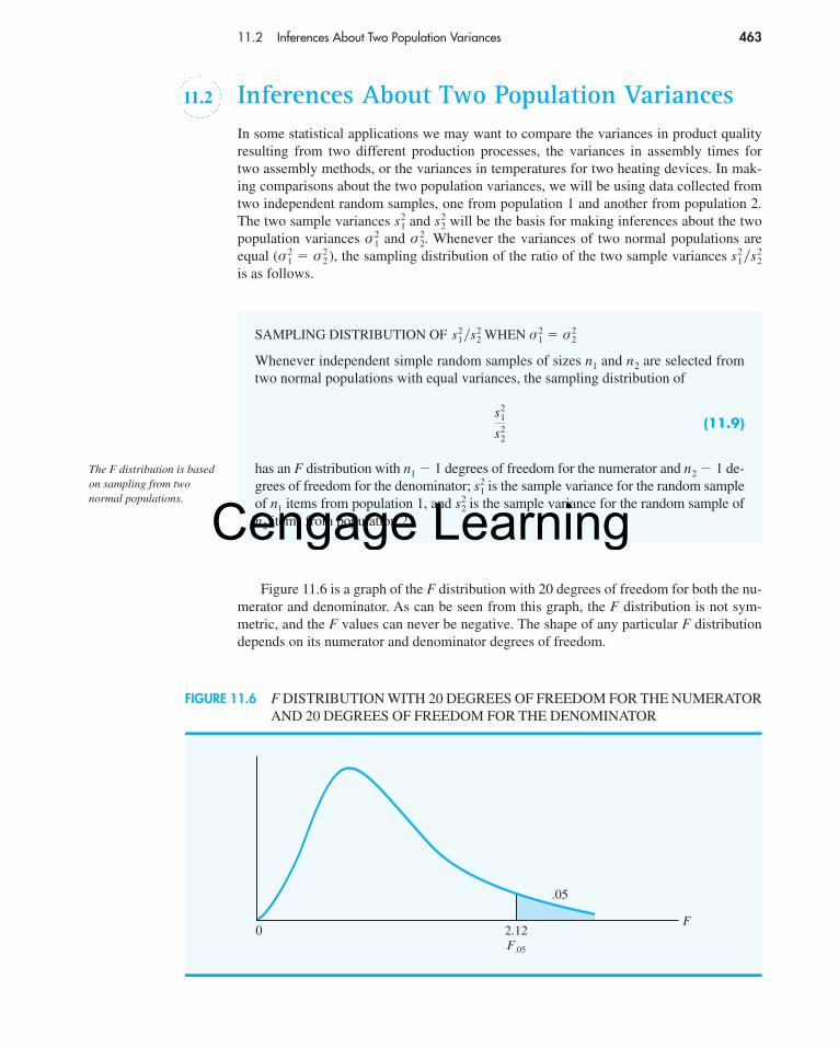
FIGURE 11.6 F DISTRIBUTION WITH 20 DEGREES OF FREEDOM FOR THE NUMERATORAND 20 DEGREES OF FREEDOM FOR THE DENOMINATOR
The F distribution is basedon sampling from twonormal populations.
SAMPLING DISTRIBUTION OF WHEN
Whenever independent simple random samples of sizes n1 and n2 are selected fromtwo normal populations with equal variances, the sampling distribution of
(11.9)
has an F distribution with n1 � 1 degrees of freedom for the numerator and n2 � 1 de-grees of freedom for the denominator; is the sample variance for the random sampleof n1 items from population 1, and is the sample variance for the random sample ofn2 items from population 2.
s22
s21
s21
s22
σ 21 � σ 2
2s21 �s2
2
Figure 11.6 is a graph of the F distribution with 20 degrees of freedom for both the nu-merator and denominator. As can be seen from this graph, the F distribution is not sym-metric, and the F values can never be negative. The shape of any particular F distributiondepends on its numerator and denominator degrees of freedom.
56130_11_ch11_p449-475.qxd 2/22/08 11:03 PM Page 463
Cengage Learning

464 Chapter 11 Inferences About Population Variances
We will use Fα to denote the value of F that provides an area or probability of α in theupper tail of the distribution. For example, as noted in Figure 11.6, F.05 denotes the uppertail area of .05 for an F distribution with 20 degrees of freedom for the numerator and 20 degrees of freedom for the denominator. The specific value of F.05 can be found by refer-ring to the F distribution table, a portion of which is shown in Table 11.3. Using 20 degreesof freedom for the numerator, 20 degrees of freedom for the denominator, and the row cor-responding to an area of .05 in the upper tail, we find F.05 � 2.12. Note that the table canbe used to find F values for upper tail areas of .10, .05, .025, and .01. See Table 4 of Ap-pendix B for a more extensive table for the F distribution.
Denominator Area in Numerator Degrees of FreedomDegrees Upper
of Freedom Tail 10 15 20 25 3010 .10 2.32 2.24 2.20 2.17 2.16
.05 2.98 2.85 2.77 2.73 2.70
.025 3.72 3.52 3.42 3.35 3.31
.01 4.85 4.56 4.41 4.31 4.25
15 .10 2.06 1.97 1.92 1.89 1.87.05 2.54 2.40 2.33 2.28 2.25.025 3.06 2.86 2.76 2.69 2.64.01 3.80 3.52 3.37 3.28 3.21
20 .10 1.94 1.84 1.79 1.76 1.74.05 2.35 2.20 2.12 2.07 2.04.025 2.77 2.57 2.46 2.40 2.35.01 3.37 3.09 2.94 2.84 2.78
25 .10 1.87 1.77 1.72 1.68 1.66.05 2.24 2.09 2.01 1.96 1.92.025 2.61 2.41 2.30 2.23 2.18.01 3.13 2.85 2.70 2.60 2.54
30 .10 1.82 1.72 1.67 1.63 1.61.05 2.16 2.01 1.93 1.88 1.84.025 2.51 2.31 2.20 2.12 2.07.01 2.98 2.70 2.55 2.45 2.39
Note: A more extensive table is provided as Table 4 of Appendix B.
TABLE 11.3 SELECTED VALUES FROM THE F DISTRIBUTION TABLE
Area orprobability
αF0
56130_11_ch11_p449-475.qxd 2/22/08 11:03 PM Page 464
Cengage Learning
11.2 Inferences About Two Population Variances 465
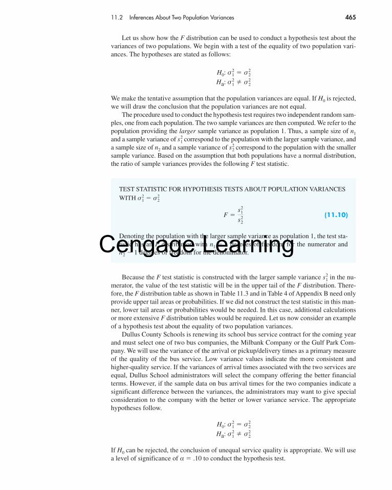
TEST STATISTIC FOR HYPOTHESIS TESTS ABOUT POPULATION VARIANCESWITH
(11.10)
Denoting the population with the larger sample variance as population 1, the test sta-tistic has an F distribution with n1 � 1 degrees of freedom for the numerator andn2 � 1 degrees of freedom for the denominator.
F �s2
1
s22
σ 21 � σ 2
2
Let us show how the F distribution can be used to conduct a hypothesis test about thevariances of two populations. We begin with a test of the equality of two population vari-ances. The hypotheses are stated as follows:
We make the tentative assumption that the population variances are equal. If H0 is rejected,we will draw the conclusion that the population variances are not equal.
The procedure used to conduct the hypothesis test requires two independent random sam-ples, one from each population. The two sample variances are then computed. We refer to thepopulation providing the larger sample variance as population 1. Thus, a sample size of n1
and a sample variance of correspond to the population with the larger sample variance, anda sample size of n2 and a sample variance of correspond to the population with the smallersample variance. Based on the assumption that both populations have a normal distribution,the ratio of sample variances provides the following F test statistic.
s22
s21
H0:
Ha: σ 2
1 � σ 22
σ 21 � σ 2
2
Because the F test statistic is constructed with the larger sample variance in the nu-merator, the value of the test statistic will be in the upper tail of the F distribution. There-fore, the F distribution table as shown in Table 11.3 and in Table 4 of Appendix B need onlyprovide upper tail areas or probabilities. If we did not construct the test statistic in this man-ner, lower tail areas or probabilities would be needed. In this case, additional calculationsor more extensive F distribution tables would be required. Let us now consider an exampleof a hypothesis test about the equality of two population variances.
Dullus County Schools is renewing its school bus service contract for the coming yearand must select one of two bus companies, the Milbank Company or the Gulf Park Com-pany. We will use the variance of the arrival or pickup/delivery times as a primary measureof the quality of the bus service. Low variance values indicate the more consistent andhigher-quality service. If the variances of arrival times associated with the two services areequal, Dullus School administrators will select the company offering the better financialterms. However, if the sample data on bus arrival times for the two companies indicate asignificant difference between the variances, the administrators may want to give specialconsideration to the company with the better or lower variance service. The appropriatehypotheses follow.
If H0 can be rejected, the conclusion of unequal service quality is appropriate. We will usea level of significance of α � .10 to conduct the hypothesis test.
H0:
Ha: σ 2
1 � σ 22
σ 21 � σ 2
2
s21
56130_11_ch11_p449-475.qxd 2/22/08 11:03 PM Page 465
Cengage Learning
466 Chapter 11 Inferences About Population Variances
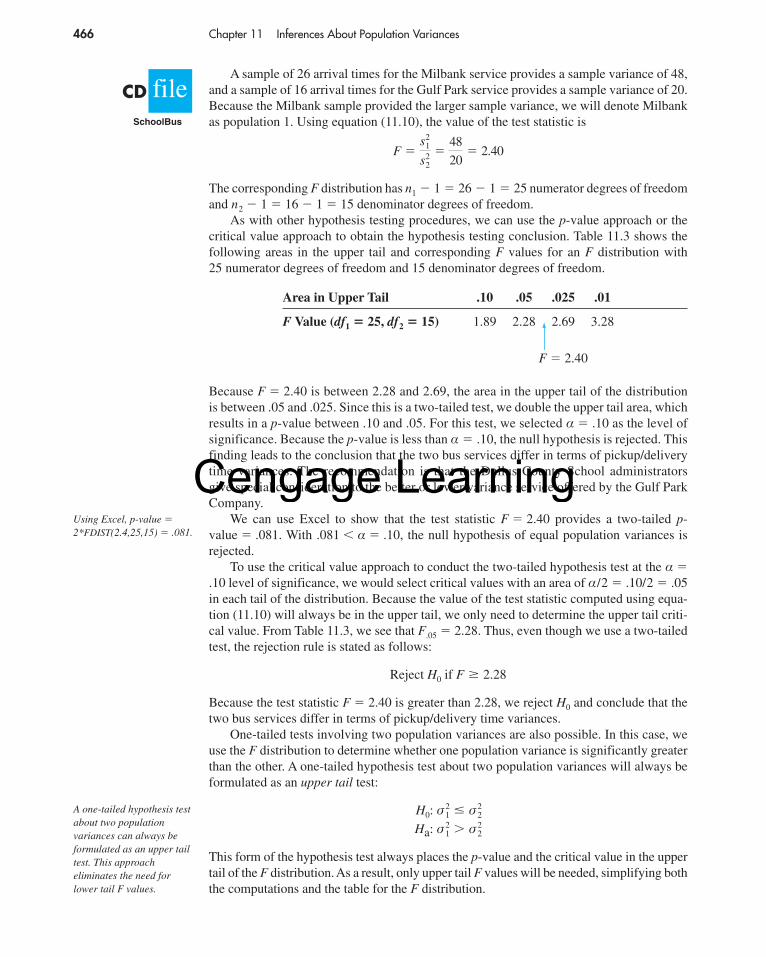
A sample of 26 arrival times for the Milbank service provides a sample variance of 48,and a sample of 16 arrival times for the Gulf Park service provides a sample variance of 20.Because the Milbank sample provided the larger sample variance, we will denote Milbankas population 1. Using equation (11.10), the value of the test statistic is
The corresponding F distribution has n1 � 1 � 26 � 1 � 25 numerator degrees of freedomand n2 � 1 � 16 � 1 � 15 denominator degrees of freedom.
As with other hypothesis testing procedures, we can use the p-value approach or thecritical value approach to obtain the hypothesis testing conclusion. Table 11.3 shows thefollowing areas in the upper tail and corresponding F values for an F distribution with 25 numerator degrees of freedom and 15 denominator degrees of freedom.
F �s2
1
s22
�48
20� 2.40
A one-tailed hypothesis testabout two populationvariances can always beformulated as an upper tailtest. This approacheliminates the need forlower tail F values.
fileCDSchoolBus
Area in Upper Tail .10 .05 .025 .01
F Value (df1 � 25, df2 � 15) 1.89 2.28 2.69 3.28
F � 2.40
Because F � 2.40 is between 2.28 and 2.69, the area in the upper tail of the distributionis between .05 and .025. Since this is a two-tailed test, we double the upper tail area, whichresults in a p-value between .10 and .05. For this test, we selected α � .10 as the level ofsignificance. Because the p-value is less than α � .10, the null hypothesis is rejected. Thisfinding leads to the conclusion that the two bus services differ in terms of pickup/deliverytime variances. The recommendation is that the Dullus County School administratorsgive special consideration to the better or lower variance service offered by the Gulf ParkCompany.
We can use Excel to show that the test statistic F � 2.40 provides a two-tailed p-value � .081. With .081 � α � .10, the null hypothesis of equal population variances isrejected.
To use the critical value approach to conduct the two-tailed hypothesis test at the α �.10 level of significance, we would select critical values with an area of α/2 � .10/2 � .05in each tail of the distribution. Because the value of the test statistic computed using equa-tion (11.10) will always be in the upper tail, we only need to determine the upper tail criti-cal value. From Table 11.3, we see that F.05 � 2.28. Thus, even though we use a two-tailedtest, the rejection rule is stated as follows:
Because the test statistic F � 2.40 is greater than 2.28, we reject H0 and conclude that thetwo bus services differ in terms of pickup/delivery time variances.
One-tailed tests involving two population variances are also possible. In this case, weuse the F distribution to determine whether one population variance is significantly greaterthan the other. A one-tailed hypothesis test about two population variances will always beformulated as an upper tail test:
This form of the hypothesis test always places the p-value and the critical value in the uppertail of the F distribution. As a result, only upper tail F values will be needed, simplifying boththe computations and the table for the F distribution.
H0:
Ha: σ 2
1 � σ 22
σ 21 � σ 2
2
Reject H0 if F � 2.28
Using Excel, p-value �
2*FDIST(2.4,25,15) � .081.
56130_11_ch11_p449-475.qxd 2/22/08 11:03 PM Page 466
Cengage Learning
11.2 Inferences About Two Population Variances 467
Let us demonstrate the use of the F distribution to conduct a one-tailed test about thevariances of two populations by considering a public opinion survey. Samples of 31 menand 41 women will be used to study attitudes about current political issues. The researcherconducting the study wants to test to see whether the sample data indicate that women showa greater variation in attitude on political issues than men. In the form of the one-tailed hy-pothesis test given previously, women will be denoted as population 1 and men will be de-noted as population 2. The hypothesis test will be stated as follows:
A rejection of H0 gives the researcher the statistical support necessary to conclude thatwomen show a greater variation in attitude on political issues.
With the sample variance for women in the numerator and the sample variance for menin the denominator, the F distribution will have n1 � 1 � 41 � 1 � 40 numerator degreesof freedom and n2 � 1 � 31 � 1 � 30 denominator degrees of freedom. We will use alevel of significance α � .05 to conduct the hypothesis test. The survey results provide asample variance of for women and a sample variance of for men. The teststatistic is as follows:
Referring to Table 4 in Appendix B, we find that an F distribution with 40 numerator degreesof freedom and 30 denominator degrees of freedom has F.10 � 1.57. Because the test statisticF � 1.50 is less than 1.57, the area in the upper tail must be greater than .10. Thus, we canconclude that the p-value is greater than .10. Excel can be used to show that F � 1.50 pro-vides a p-value � .1256. Because the p-value � α � .05, H0 cannot be rejected. Hence, thesample results do not support the conclusion that women show greater variation in attitude onpolitical issues than men. Table 11.4 provides a summary of hypothesis tests about two popu-lation variances.
F �s2
1
s22
�120
80� 1.50
s22 � 80s2
1 � 120
H0:
Ha: σ2
women � σ2men
σ2women � σ2
men
Upper Tail Test Two-Tailed Test
Hypotheses
Note: Population 1has the largersample variance
Test Statistic
Rejection Rule: Reject H0 if Reject H0 ifp-value Approach p-value � α p-value � α
Rejection Rule: Reject H0 if Reject H0 ifCritical Value F � Fα F � Fα/2
Approach
F �s2
1
s22
F �s2
1
s22
H0:
Ha: σ 2
1 � σ 22
σ 21 � σ 2
2
H0:
Ha: σ 2
1 � σ 22
σ 21 � σ 2
2
TABLE 11.4 SUMMARY OF HYPOTHESIS TESTS ABOUT TWO POPULATION VARIANCES
Using Excel, p-value �
2*FDIST(1.5,40,30) �
.1256.
56130_11_ch11_p449-475.qxd 2/22/08 11:03 PM Page 467
Cengage Learning

468 Chapter 11 Inferences About Population Variances
Using Excel to Conduct a Hypothesis TestExcel’s F-Test Two-Sample for Variances tool can be used to conduct a hypothesis testcomparing the variances of two populations. We illustrate by using Excel to conduct thetwo-tailed hypothesis test for the Dullus County School Bus study. Refer to Figure 11.7 andthe dialog box in Figure 11.8 as we describe the tasks involved.
Enter Data: Column A contains the sample of 26 arrival times for the Milbank Companyand column B contains the sample of 16 arrival times for the Gulf Park Company.
Apply Tools: The following steps describe how to use Excel’s F-Test Two-Sample forVariances tool.
Step 1. Click the Data tab on the RibbonStep 2. In the Analysis group, click Data AnalysisStep 3. When the Data Analysis dialog box appears,
Choose F-Test Two-Sample for Variances from the list of Analysis ToolsClick OK
Step 4. When the F-Test Two-Sample for Variances dialog box appears (Figure 11.8):Enter A1:A27 in the Variable 1 Range boxEnter B1:B17 in the Variable 2 Range boxSelect LabelsEnter .05 in the Alpha box
(Note: This Excel procedure uses alpha as the area in the upper tail.)Select Output Range and enter D1 in the boxClick OK
The output, P(F��f) one-tail �.0405, is the one-tail area associated with the test statisticF � 2.401. Thus, the two-tailed p-value is 2(.0405) � .081; we reject the null hypothesis atthe .10 level of significance. If the hypothesis test had been a one-tail test (with α � .05), theone-tail area in cell E9 would provide the p-value directly. We would not need to double it.
FIGURE 11.7 HYPOTHESIS TEST COMPARING VARIANCE IN PICKUP TIMES FOR TWO SCHOOLBUS SERVICES
A B C D E F G1 Milbank Gulf Park F-Test Two-Sample for Variances2 35.9 21.63 29.9 20.5 Milbank Gulf Park4 31.2 23.3 Mean 20.2308 20.24385 16.2 18.8 Variance 48.0206 20.00006 19.0 17.2 Observations 26 167 15.9 7.7 df 25 158 18.8 18.6 F 2.40109 22.2 18.7 P(F<=f) one-tail 0.040510 19.9 20.4 F Critical one-tail 2.279711 16.4 22.416 18.0 27.917 28.1 20.818 12.126 15.227 28.228
Note: Rows 12–15 and19–25 are hidden.
fileCDSchoolBus
56130_11_ch11_p449-475.qxd 2/22/08 11:03 PM Page 468
Cengage Learning

11.2 Inferences About Two Population Variances 469
NOTES AND COMMENTS
Research confirms the fact that the F distribution issensitive to the assumption of normal populations.The F distribution should not be used unless it is
reasonable to assume that both populations are atleast approximately normally distributed.
Exercises
Methods13. Find the following F distribution values from Table 4 of Appendix B.
a. F.05 with degrees of freedom 5 and 10b. F.025 with degrees of freedom 20 and 15c. F.01 with degrees of freedom 8 and 12d. F.10 with degrees of freedom 10 and 20
14. A sample of 16 items from population 1 has a sample variance � 5.8 and a sample of21 items from population 2 has a sample variance � 2.4. Test the following hypothesesat the .05 level of significance.
a. What is your conclusion using the p-value approach?b. Repeat the test using the critical value approach.
15. Consider the following hypothesis test.
H0:
Ha: σ 2
1 � σ 22
σ 21 � σ 2
2
H0:
Ha: σ 2
1 � σ 22
σ 21 � σ 2
2
s22
s21
FIGURE 11.8 DIALOG BOX FOR F-TEST TWO-SAMPLE FOR VARIANCES
testSELF
56130_11_ch11_p449-475.qxd 2/22/08 11:03 PM Page 469
Cengage Learning

470 Chapter 11 Inferences About Population Variances
a. What is your conclusion if n1 � 21, � 8.2, n2 � 26, and � 4.0? Use α � .05 andthe p-value approach.
b. Repeat the test using the critical value approach.
Applications16. Media Metrix and Jupiter Communications gathered data on the time adults and the time
teens spend online during a month (USA Today, September 14, 2000). The study concludedthat on average, adults spend more time online than teens. Assume that a follow-up studysampled 26 adults and 30 teens. The standard deviations of the time online during a monthwere 94 minutes and 58 minutes, respectively. Do the sample results support the conclu-sion that adults have a greater variance in online time than teens? Use α � .01. What isthe p-value?
17. Most individuals are aware of the fact that the average annual repair cost for an auto-mobile depends on the age of the automobile. A researcher is interested in finding outwhether the variance of the annual repair costs also increases with the age of the automo-bile. A sample of 26 automobiles 4 years old showed a sample standard deviation for annual repair costs of $170 and a sample of 25 automobiles 2 years old showed a samplestandard deviation for annual repair costs of $100.a. State the null and alternative versions of the research hypothesis that the variance in
annual repair costs is larger for the older automobiles.b. At a .01 level of significance, what is your conclusion? What is the p-value? Discuss
the reasonableness of your findings.
18. The standard deviation in the 12-month earnings per share for 10 companies in the airlineindustry was 4.27 and the standard deviation in the 12-month earnings per share for 7 com-panies in the automotive industry was 2.27 (BusinessWeek, August 14, 2000). Conduct atest for equal variances at α � .05. What is your conclusion about the variability in earn-ings per share for the airline industry and the automotive industry?
19. The variance in a production process is an important measure of the quality of the process.A large variance often signals an opportunity for improvement in the process by findingways to reduce the process variance. Conduct a statistical test to determine whether thereis a significant difference between the variances in the bag weights for the two machines.Use a .05 level of significance. What is your conclusion? Which machine, if either, pro-vides the greater opportunity for quality improvements?
s22s2
1
Machine 1 2.95 3.45 3.50 3.75 3.48 3.26 3.33 3.203.16 3.20 3.22 3.38 3.90 3.36 3.25 3.283.20 3.22 2.98 3.45 3.70 3.34 3.18 3.353.12
Machine 2 3.22 3.30 3.34 3.28 3.29 3.25 3.30 3.273.38 3.34 3.35 3.19 3.35 3.05 3.36 3.283.30 3.28 3.30 3.20 3.16 3.33
fileCDBags
20. On the basis of data provided by a Romac salary survey, the variance in annual salaries forseniors in public accounting firms is approximately 2.1 and the variance in annual salariesfor managers in public accounting firms is approximately 11.1. The salary data wereprovided in thousands of dollars. Assuming that the salary data were based on samples of25 seniors and 26 managers, test the hypothesis that the population variances in the salariesare equal. At a .05 level of significance, what is your conclusion?
testSELF
56130_11_ch11_p449-475.qxd 2/22/08 11:03 PM Page 470
Cengage Learning

Key Formulas 471
21. Fidelity Magellan is a large cap growth mutual fund and Fidelity Small Cap Stock is a smallcap growth mutual fund (Morningstar Funds 500, 2006). The standard deviation for bothfunds was computed based on a sample of size 26. For Fidelity Magellan, the sample stan-dard deviation is 8.89%; for Fidelity Small Cap Stock, the sample standard deviation is13.03%. Financial analysts often use the standard deviation as a measure of risk. Conducta hypothesis test to determine whether the small cap growth fund is riskier than the largecap growth fund. Use α � .05 as the level of significance.
22. A research hypothesis is that the variance of stopping distances of automobiles on wetpavement is substantially greater than the variance of stopping distances of automobileson dry pavement. In the research study, 16 automobiles traveling at the same speeds aretested for stopping distances on wet pavement and then tested for stopping distances ondry pavement. On wet pavement, the standard deviation of stopping distances is 32 feet.On dry pavement, the standard deviation is 16 feet.a. At a .05 level of significance, do the sample data justify the conclusion that the vari-
ance in stopping distances on wet pavement is greater than the variance in stoppingdistances on dry pavement? What is the p-value?
b. What are the implications of your statistical conclusions in terms of driving safetyrecommendations?
Summary
In this chapter we presented statistical procedures that can be used to make inferences aboutpopulation variances. In the process we introduced two new probability distributions: thechi-square distribution and the F distribution. The chi-square distribution can be used as the basis for interval estimation and hypothesis tests about the variance of a normal popu-lation, and the F distribution can be used to conduct hypothesis tests about the variances oftwo normal populations. In particular, we showed that with independent simple randomsamples of sizes n1 and n2 selected from two normal populations with equal variances
the sampling distribution of the ratio of the two sample variances has an F distribution with n1 � 1 degrees of freedom for the numerator and n2 � 1 degrees of free-dom for the denominator.
Key Formulas
Interval Estimate of a Population Variance
(11.7)
Test Statistic for Hypothesis Tests About a Population Variance
(11.8)
Test Statistic for Hypothesis Tests About Population Variances with
(11.10)F �s2
1
s22
σ 21 � σ
22
� 2 �(n � 1)s2
σ 20
(n � 1)s2
� 2α/2
� σ 2 �(n � 1)s2
� 2(1�α/2)
s21 �s2
2σ 21 � σ 2
2,
56130_11_ch11_p449-475.qxd 2/22/08 11:03 PM Page 471
Cengage Learning

472 Chapter 11 Inferences About Population Variances
Supplementary Exercises
23. Because of staffing decisions, managers of the Gibson-Marimont Hotel are interested inthe variability in the number of rooms occupied per day during a particular season of theyear. A sample of 20 days of operation shows a sample mean of 290 rooms occupied perday and a sample standard deviation of 30 rooms.a. What is the point estimate of the population variance?b. Provide a 90% confidence interval estimate of the population variance.c. Provide a 90% confidence interval estimate of the population standard deviation.
24. Initial public offerings (IPOs) of stocks are on average underpriced. The standard devia-tion measures the dispersion, or variation, in the underpricing-overpricing indicator. Asample of 13 Canadian IPOs that were subsequently traded on the Toronto Stock Exchangehad a standard deviation of 14.95. Develop a 95% confidence interval estimate of the pop-ulation standard deviation for the underpricing-overpricing indicator.
25. The estimated daily living costs for an executive traveling to various major cities follow.The estimates include a single room at a four-star hotel, beverages, breakfast, taxi fares,and incidental costs.
City Daily Living Cost ($) City Daily Living Cost ($)
Bangkok 242.87 Madrid 283.56Bogotá 260.93 Mexico City 212.00Bombay 139.16 Milan 284.08Cairo 194.19 Paris 436.72Dublin 260.76 Rio de Janeiro 240.87Frankfurt 355.36 Seoul 310.41Hong Kong 346.32 Tel Aviv 223.73Johannesburg 165.37 Toronto 181.25Lima 250.08 Warsaw 238.20London 326.76 Washington, D.C. 250.61
fileCDTravel
a. Compute the sample mean.b. Compute the sample standard deviation.c. Compute a 95% confidence interval for the population standard deviation.
26. Part variability is critical in the manufacturing of ball bearings. Large variances in the sizeof the ball bearings cause bearing failure and rapid wearout. Production standards call fora maximum variance of .0001 when the bearing diameters are measured in inches. Asample of 15 bearings shows a sample standard deviation of .014 inches.a. Use α � .10 to determine whether the sample indicates that the maximum acceptable
variance is being exceeded.b. Compute the 90% confidence interval estimate of the variance of the ball bearings in
the population.
27. The filling weight for boxes of cereal is designed to have a variance .02 ounces or less. Asample of 41 boxes of cereal shows a sample standard deviation of .16 ounces. Use α � .05to determine whether the variance in the cereal box filling weight is exceeding the designspecification.
28. City Trucking, Inc., claims consistent delivery times for its routine customer deliveries. Asample of 22 truck deliveries shows a sample variance of 1.5 minutes. Test to determinewhether H0: σ
2 � 1 can be rejected. Use α � .10.
29. A sample of 9 days over the past 6 months showed that a dentist treated the following num-bers of patients: 22, 25, 20, 18, 15, 22, 24, 19, and 26. If the number of patients seen per
56130_11_ch11_p449-475.qxd 2/22/08 11:03 PM Page 472
Cengage Learning

Case Problem Air Force Training Program 473
Case Problem Air Force Training ProgramAn Air Force introductory course in electronics uses a personalized system of instructionwhereby each student views a videotaped lecture and then is given a programmed instruc-tion text. The students work independently with the text until they have completed the train-ing and passed a test. Of concern is the varying pace at which the students complete thisportion of their training program. Some students are able to cover the programmed in-struction text relatively quickly, whereas other students work much longer with the text andrequire additional time to complete the course. The fast students wait until the slow studentscomplete the introductory course before the entire group proceeds together with otheraspects of their training.
A proposed alternative system involves use of computer-assisted instruction. In thismethod, all students view the same videotaped lecture and then each is assigned to a com-puter terminal for further instruction. The computer guides the student, working indepen-dently, through the self-training portion of the course.
day is normally distributed, would an analysis of these sample data reject the hypothesisthat the variance in the number of patients seen per day is equal to 10? Use a .10 level ofsignificance. What is your conclusion?
30. A sample standard deviation for the number of passengers taking a particular airline flightis 8. A 95% confidence interval estimate of the population standard deviation is 5.86 pas-sengers to 12.62 passengers.a. Was a sample size of 10 or 15 used in the statistical analysis?b. Suppose the sample standard deviation of s � 8 was based on a sample of 25 flights.
What change would you expect in the confidence interval for the populationstandard deviation? Compute a 95% confidence interval estimate of σ with a sam-ple size of 25.
31. Each day the major stock markets have a group of leading gainers in price (stocks that goup the most). On one day the standard deviation in the percentage change for a sample of10 NASDAQ leading gainers was 15.8. On the same day, the standard deviation in the per-centage change for a sample of 10 NYSE leading gainers was 7.9 (USA Today, September14, 2000). Conduct a test for equal population variances to see whether it can be concludedthat there is a difference in the volatility of the leading gainers on the two exchanges. Useα � .10. What is your conclusion?
32. The grade point averages of 352 students who completed a college course in financial ac-counting have a standard deviation of .940. The grade point averages of 73 students whodropped out of the same course have a standard deviation of .797. Do the data indicate adifference between the variances of grade point averages for students who completed a fi-nancial accounting course and students who dropped out? Use a .05 level of significance.Note: F.025 with 351 and 72 degrees of freedom is 1.466.
33. The accounting department analyzes the variance of the weekly unit costs reported by twoproduction departments. A sample of 16 cost reports for each of the two departments showscost variances of 2.3 and 5.4, respectively. Is this sample sufficient to conclude that the twoproduction departments differ in terms of unit cost variance? Use α � .10.
34. Two new assembly methods are tested and the variances in assembly times are reported.Use α � .10 and test for equality of the two population variances.
Method A Method B
Sample Size
Sample Variation s22 � 12s2
1 � 25
n 2 � 25n1 � 31
56130_11_ch11_p449-475.qxd 2/22/08 11:03 PM Page 473
Cengage Learning
474 Chapter 11 Inferences About Population Variances
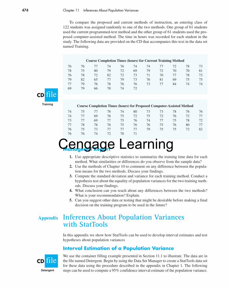
To compare the proposed and current methods of instruction, an entering class of 122 students was assigned randomly to one of the two methods. One group of 61 studentsused the current programmed-text method and the other group of 61 students used the pro-posed computer-assisted method. The time in hours was recorded for each student in thestudy. The following data are provided on the CD that accompanies this text in the data setnamed Training.
Course Completion Times (hours) for Current Training Method
76 76 77 74 76 74 74 77 72 78 7378 75 80 79 72 69 79 72 70 70 8176 78 72 82 72 73 71 70 77 78 7379 82 65 77 79 73 76 81 69 75 7577 79 76 78 76 76 73 77 84 74 7469 79 66 70 74 72
Course Completion Times (hours) for Proposed Computer-Assisted Method
74 75 77 78 74 80 73 73 78 76 7674 77 69 76 75 72 75 72 76 72 7773 77 69 77 75 76 74 77 75 78 7277 78 78 76 75 76 76 75 76 80 7776 75 73 77 77 77 79 75 75 72 8276 76 74 72 78 71
fileCDTraining
Managerial Report1. Use appropriate descriptive statistics to summarize the training time data for each
method. What similarities or differences do you observe from the sample data?2. Use the methods of Chapter 10 to comment on any difference between the popula-
tion means for the two methods. Discuss your findings.3. Compute the standard deviation and variance for each training method. Conduct a
hypothesis test about the equality of population variances for the two training meth-ods. Discuss your findings.
4. What conclusion can you reach about any differences between the two methods?What is your recommendation? Explain.
5. Can you suggest other data or testing that might be desirable before making a finaldecision on the training program to be used in the future?
Appendix Inferences About Population Variances with StatToolsIn this appendix we show how StatTools can be used to develop interval estimates and testhypotheses about population variances
Interval Estimation of a Population VarianceWe use the container filling example presented in Section 11.1 to illustrate. The data are inthe file named Detergent. Begin by using the Data Set Manager to create a StatTools data setfor these data using the procedure described in the appendix in Chapter 1. The followingsteps can be used to compute a 95% confidence interval estimate of the population variance.
fileCDDetergent
56130_11_ch11_p449-475.qxd 2/22/08 11:03 PM Page 474
Cengage Learning

Step 1. Click the StatTools tab on the RibbonStep 2. In the Analyses group, click Statistical InferenceStep 3. Choose the Confidence Interval optionStep 4. When the StatTools—Confidence Interval dialog box appears,
For Analysis Type, choose One-Sample AnalysisIn the Variables section, select OuncesIn the Confidence Intervals to Calculate section,
Select the For the Standard Deviation optionSelect 95% for the Confidence Level
Click OK
The StatTools output will provide a 95% confidence interval for the population standarddeviation. To compute the corresponding confidence interval for the population variance,simply square the lower and upper limits on the StatTools output.
Hypothesis TestingWe use the St. Louis Metro Bus Company example presented in Section 11.1 to illustrate.The data are in the file named BusTimes. Begin by using the Data Set Manager to create aStatTools data set for these data using the procedure described in the appendix in Chapter 1.The following steps can be used to test the hypothesis H0: σ 2 � 4 against Ha: σ 2 � 4. Be-cause the StatTools procedure works with the standard deviation, this is equivalent to test-ing the hypotheses H0: σ � 2 against Ha: σ � 2.
Step 1. Click the StatTools tab on the RibbonStep 2. In the Analyses group, click Statistical InferenceStep 3. Choose the Hypothesis Test optionStep 4. When the StatTools—Hypothesis Test dialog box appears,
For Analysis Type, choose One-Sample AnalysisIn the Variables section, select TimesIn the Hypothesis Tests to Perform section,
Select the Standard Deviation optionEnter 2 in the Null Hypothesis Value boxSelect the Greater Than Null Value (One-Tailed Test) in the Alter-
native Hypothesis Type boxClick OK
The hypothesis testing results will appear.
Appendix Inferences About Population Variances with StatTools 475
fileCDBusTimes
56130_11_ch11_p449-475.qxd 2/22/08 11:03 PM Page 475
Cengage Learning

Tests of Goodness of Fitand Independence
CONTENTS
STATISTICS IN PRACTICE: UNITED WAY
12.1 GOODNESS OF FIT TEST: AMULTINOMIAL POPULATIONUsing Excel to Conduct a
Goodness of Fit Test
12.2 TEST OF INDEPENDENCEUsing Excel to Conduct a Test of
Independence
12.3 GOODNESS OF FIT TEST:POISSON AND NORMALDISTRIBUTIONSPoisson DistributionUsing Excel to Conduct a
Goodness of Fit TestNormal DistributionUsing Excel to Conduct a
Goodness of Fit Test
CHAPTER 12
56130_12_ch12_p476-507.qxd 2/22/08 10:51 PM Page 476
Cengage Learning

Chapter 12 Tests of Goodness of Fit and Independence 477
United Way of Greater Rochester is a nonprofit organi-zation dedicated to improving the quality of life for allpeople in the seven counties it serves by meeting thecommunity’s most important human care needs.
The annual United Way/Red Cross fund-raisingcampaign, conducted each spring, funds hundreds ofprograms offered by more than 200 service providers.These providers meet a wide variety of human needs—physical, mental, and social—and serve people of allages, backgrounds, and economic means.
Because of enormous volunteer involvement, UnitedWay of Greater Rochester is able to hold its operatingcosts at just eight cents of every dollar raised.
The United Way of Greater Rochester decided toconduct a survey to learn more about community percep-tions of charities. Focus-group interviews were held withprofessional, service, and general worker groups to getpreliminary information on perceptions. The informationobtained was then used to help develop the questionnairefor the survey. The questionnaire was pretested, modi-fied, and distributed to 440 individuals; 323 completedquestionnaires were obtained.
A variety of descriptive statistics, includingfrequency distributions and crosstabulations, wereprovided from the data collected. An important part ofthe analysis involved the use of contingency tables andchi-square tests of independence. One use of suchstatistical tests was to determine whether perceptionsof administrative expenses were independent ofoccupation.
The hypotheses for the test of independence were:
H0: Perception of United Way administrativeexpenses is independent of the occupation ofthe respondent.
Ha: Perception of United Way administrativeexpenses is not independent of the occupationof the respondent.
Two questions in the survey provided the data for thestatistical test. One question obtained data on perceptionsof the percentage of funds going to administrative ex-penses (up to 10%, 11–20%, and 21% or more). The otherquestion asked for the occupation of the respondent.
The chi-square test at a .05 level of significance ledto rejection of the null hypothesis of independence andto the conclusion that perceptions of United Way’s ad-ministrative expenses did vary by occupation. Actual ad-ministrative expenses were less than 9%, but 35% of therespondents perceived that administrative expenses were21% or more. Hence, many had inaccurate perceptionsof administrative costs. In this group, production-line,clerical, sales, and professional-technical employees hadmore inaccurate perceptions than other groups.
The community perceptions study helped UnitedWay of Greater Rochester to develop adjustments to itsprogram and fund-raising activities. In this chapter, youwill learn how a statistical test of independence, such asthat described here, is conducted.
Statistical surveys help United Way adjust itsprogram to better meet the needs of the peopleit serves. Ed Bock/Corbis
UNITED WAY*ROCHESTER, NEW YORK
STATISTICS in PRACTICE
*The authors are indebted to Dr. Philip R. Tyler, Marketing Consultant tothe United Way, for providing this Statistics in Practice.
In Chapter 11 we showed how the chi-square distribution could be used in estimation andin hypothesis tests about a population variance. In Chapter 12, we introduce two additionalhypothesis testing procedures, both based on the use of the chi-square distribution. Likeother hypothesis testing procedures, these tests compare sample results with those that areexpected when the null hypothesis is true. The conclusion of the hypothesis test is based onhow “close” the sample results are to the expected results.
56130_12_ch12_p476-507.qxd 2/26/08 10:45 AM Page 477
Cengage Learning

478 Chapter 12 Tests of Goodness of Fit and Independence
In the following section we introduce a goodness of fit test for a multinomial popula-tion. Later we discuss the test for independence using contingency tables and then showgoodness of fit tests for the Poisson and normal distributions.
12.1 Goodness of Fit Test: A Multinomial PopulationIn this section we consider the case in which each element of a population is assigned to oneand only one of several classes or categories. Such a population is a multinomial population.The multinomial distribution can be thought of as an extension of the binomial distribution tothe case of three or more categories of outcomes. On each trial of a multinomial experiment,one and only one of the outcomes occurs. Each trial of the experiment is assumed to be inde-pendent, and the probabilities of the outcomes remain the same for each trial.
As an example, consider the market share study being conducted by Scott MarketingResearch. Over the past year market shares stabilized at 30% for company A, 50% for com-pany B, and 20% for company C. Recently company C developed a “new and improved”product to replace its current entry in the market. Company C retained Scott MarketingResearch to determine whether the new product will alter market shares.
In this case, the population of interest is a multinomial population; each customer is clas-sified as buying from company A, company B, or company C. Thus, we have a multinomialpopulation with three outcomes. Let us use the following notation for the proportions:
Scott Marketing Research will conduct a sample survey and compute the proportionpreferring each company’s product. A hypothesis test will then be conducted to see whetherthe new product caused a change in market shares. For the null hypothesis, we assume thatcompany C’s new product will not alter the market shares. The null and alternativehypotheses are stated as follows:
If the sample results lead to the rejection of H0, Scott Marketing Research will have evi-dence that the introduction of the new product affects market shares.
Let us assume that the market research firm has used a consumer panel of 200 customersfor the study. Each individual was asked to specify a purchase preference among the threealternatives: company A’s product, company B’s product, and company C’s new product.The 200 responses are summarized here.
H0:
Ha:
pA � .30, pB � .50, and pC � .20
The population proportions are notpA � .30, pB � .50, and pC � .20
pA �
pB �
pC �
market share for company A
market share for company B
market share for company C
The assumptions for themultinomial experimentparallel those for thebinomial experiment withthe exception that themultinomial has three ormore outcomes per trial.
Observed Frequency
Company A’s Company B’s Company C’sProduct Product New Product
48 98 54
The consumer panel of 200 customers in whicheach individual is askedto select one of threealternatives is equivalent toa multinomial experimentconsisting of 200 trials.
We now can perform a goodness of fit test that will determine whether the sample of200 customer purchase preferences is consistent with the null hypothesis. The goodness of
56130_12_ch12_p476-507.qxd 2/22/08 10:51 PM Page 478
Cengage Learning

12.1 Goodness of Fit Test: A Multinomial Population 479
Area in Upper Tail .10 .05 .025 .01
� 2 Value (2 df) 4.605 5.991 7.378 9.210
� 2 � 7.34
TEST STATISTIC FOR GOODNESS OF FIT
(12.1)
where
Note: The test statistic has a chi-square distribution with k � 1 degrees of freedomprovided that the expected frequencies are 5 or more for all categories.
fi �
ei �
k �
observed frequency for category i
expected frequency for category i
the number of categories
� 2 � �k
i�1
( fi � ei
)2
ei
The test for goodness of fitis always a one-tailed testwith the rejection occurringin the upper tail of the chi-square distribution.
An introduction to the chi-square distribution and the use of the chi-squaretable were presented inSection 11.1.
fit test is based on a comparison of the sample of observed results with the expected resultsunder the assumption that the null hypothesis is true. Hence, the next step is to compute ex-pected purchase preferences for the 200 customers under the assumption that pA � .30,pB � .50, and pC � .20. Doing so provides the expected results.
Thus, we see that the expected frequency for each category is found by multiplying the sample size of 200 by the hypothesized proportion for the category.
The goodness of fit test now focuses on the differences between the observed frequen-cies and the expected frequencies. Large differences between observed and expected fre-quencies cast doubt on the assumption that the hypothesized proportions or market sharesare correct. Whether the differences between the observed and expected frequencies are“large” or “small” is a question answered with the aid of the following test statistic.
Let us continue with the Scott Marketing Research example and use the sample data totest the hypothesis that the multinomial population retains the proportions pA � .30, pB �.50, and pC � .20. We will use an α � .05 level of significance. Let us proceed by using theobserved and expected frequencies to compute the value of the test statistic. With the ex-pected frequencies all 5 or more, the computation of the chi-square test statistic is shownin Table 12.1. At the bottom of the last column, we see that � 2 � 7.34.
We will reject the null hypothesis if the differences between the observed and expectedfrequencies are large. Large differences between the observed and expected frequencieswill result in a large value for the test statistic. Thus the test of goodness of fit will alwaysbe an upper tail test. We can use the upper tail area for the test statistic and the p-valueapproach to determine whether the null hypothesis can be rejected. With k � 1 � 3 � 1 � 2degrees of freedom, the chi-square table (Table 3 of Appendix B) provides the following:
Expected Frequency
Company A’s Company B’s Company C’sProduct Product New Product
200(.30) � 60 200(.50) � 100 200(.20) � 40
56130_12_ch12_p476-507.qxd 2/22/08 10:51 PM Page 479
Cengage Learning
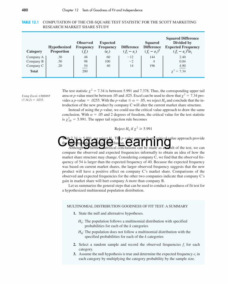
480 Chapter 12 Tests of Goodness of Fit and Independence
Squared DifferenceObserved Expected Squared Divided by
Hypothesized Frequency Frequency Difference Difference Expected FrequencyCategory Proportion ( fi) (ei) ( fi � ei) ( fi � ei)
2 ( fi � ei)2/ei
Company A .30 48 60 �12 144 2.40Company B .50 98 100 �2 4 0.04Company C .20 54 40 14 196 4.90
Total 200 � 2 � 7.34
TABLE 12.1 COMPUTATION OF THE CHI-SQUARE TEST STATISTIC FOR THE SCOTT MARKETINGRESEARCH MARKET SHARE STUDY
The test statistic �2 � 7.34 is between 5.991 and 7.378. Thus, the corresponding upper tailarea or p-value must be between .05 and .025. Excel can be used to show that �2 � 7.34 pro-vides a p-value � .0255. With the p-value � α � .05, we reject H0 and conclude that the in-troduction of the new product by company C will alter the current market share structure.
Instead of using the p-value, we could use the critical value approach to draw the sameconclusion. With α � .05 and 2 degrees of freedom, the critical value for the test statisticis The upper tail rejection rule becomes
With 7.34 � 5.991, we reject H0. The p-value approach and critical value approach providethe same hypothesis testing conclusion.
Although no further statistical conclusions can be made as a result of the test, we cancompare the observed and expected frequencies informally to obtain an idea of how themarket share structure may change. Considering company C, we find that the observed fre-quency of 54 is larger than the expected frequency of 40. Because the expected frequencywas based on current market shares, the larger observed frequency suggests that the newproduct will have a positive effect on company C’s market share. Comparisons of theobserved and expected frequencies for the other two companies indicate that company C’sgain in market share will hurt company A more than company B.
Let us summarize the general steps that can be used to conduct a goodness of fit test fora hypothesized multinomial population distribution.
Reject H0 if �2 � 5.991
� 2.05 � 5.991.
MULTINOMIAL DISTRIBUTION GOODNESS OF FIT TEST: A SUMMARY
1. State the null and alternative hypotheses.
H0: The population follows a multinomial distribution with specifiedprobabilities for each of the k categories
Ha: The population does not follow a multinomial distribution with thespecified probabilities for each of the k categories
2. Select a random sample and record the observed frequencies fi for eachcategory.
3. Assume the null hypothesis is true and determine the expected frequency ei ineach category by multiplying the category probability by the sample size.
Using Excel, CHIDIST(7.34,2) � .0255.
56130_12_ch12_p476-507.qxd 2/22/08 10:51 PM Page 480
Cengage Learning

A B C D E F G H I J K1 Customer Product Squared Diff.2 1 B Hyp. Obs. Exp. Squared Divided by3 2 A Category Proportion Freq. Freq. Diff. Diff. Exp. Freq.4 3 C Company A 0.3 =COUNTIF(B2:B201,"A") =E4*F7 =F4-G4 =H4^2 =I4/G45 4 C Company B 0.5 =COUNTIF(B2:B201,"B") =E5*F7 =F5-G5 =H5^2 =I5/G56 5 C Company C 0.2 =COUNTIF(B2:B201,"C") =E6*F7 =F6-G6 =H6^2 =I6/G67 6 A Total =SUM(F4:F6) =SUM(J4:J6)8 7 A9 8 A Number of Categories 3
10 9 C11 10 A Test Statistic =J712 11 C Degrees of Freedom =F9-113 12 B14 13 C p-value =CHIDIST(F11,F12)15 14 A
200 199 C201 200 C202
12.1 Goodness of Fit Test: A Multinomial Population 481
Using Excel to Conduct a Goodness of Fit TestExcel can be used to conduct a goodness of fit test for the Scott Marketing Research Study.Refer to Figure 12.1 as we describe the tasks involved. The formula worksheet is in thebackground; the value worksheet is in the foreground.
Enter Data: Column A is used to identify each of the 200 customers who made up the con-sumer panel in the study. Column B shows the purchase preference (A, B, or C) for eachcustomer. The hypothesized proportions, 0.3, 0.5, and 0.2, were entered into cells E4:E6.
4. Compute the value of the test statistic.
5. Rejection rule:
where α is the level of significance for the test and there are k � 1 degrees offreedom.
p-value approach:
Critical value approach:
Reject H0 if p-value � αReject H0 if �
2 � � 2α
� 2 � �k
i�1
( fi � ei)
2
ei
FIGURE 12.1 EXCEL WORKSHEET FOR GOODNESS OF FIT TEST CONCERNING MARKETSHARE CHANGE
A B C D E F G H I J K1 Customer Product Squared Diff.2 1 B Hyp. Obs. Exp. Squared Divided by3 2 A Category Proportion Freq. Freq. Diff. Diff. Exp. Freq.4 3 C Company A 0.3 48 60 -12 144 2.45 4 C Company B 0.5 98 100 -2 4 0.046 5 C Company C 0.2 54 40 14 196 4.97 6 A Total 200 7.348 7 A9 8 A Number of Categories 3
10 9 C11 10 A Test Statistic 7.3412 11 C Degrees of Freedom 213 12 B14 13 C p-value 0.025515 14 A
200 199 C201 200 C202
Note: Rows 16–199are hidden.
fileCDResearch
56130_12_ch12_p476-507.qxd 2/22/08 10:51 PM Page 481
Cengage Learning
482 Chapter 12 Tests of Goodness of Fit and Independence
Enter Functions and Formulas: The Excel formulas in cells F4:J7 are used to computethe chi-square test statistic in a fashion parallel to that shown in Table 12.1. The result is thechi-square test statistic shown in cell J7 (7.34). The number of categories, 3, was entered intocell F9 and the two inputs used by Excel’s CHIDIST function (test statistic and degrees offreedom) are in cells F11 and F12. The value computed in cell F14 using Excel’s CHIDISTfunction is the area in the upper tail of the chi-square distribution to the right of the test sta-tistic. So, this value is the appropriate p-value for our upper tail hypothesis test.
The value worksheet shows that the resulting p-value is 0.0255. Thus, with α � .05, wereject H0 and conclude that the introduction of the new product by company C will alter thecurrent market share structure.
Exercises
Methods1. Test the following hypotheses by using the � 2 goodness of fit test.
A sample of size 200 yielded 60 in category A, 120 in category B, and 20 in category C.Use α � .01 and test to see whether the proportions are as stated in H0.a. Use the p-value approach.b. Repeat the test using the critical value approach.
2. Suppose we have a multinomial population with four categories: A, B, C, and D. The nullhypothesis is that the proportion of items is the same in every category. The nullhypothesis is
A sample of size 300 yielded the following results.
Use α � .05 to determine whether H0 should be rejected. What is the p-value?
Applications3. During the first 13 weeks of the television season, the Saturday evening 8:00 p.m. to
9:00 p.m. audience proportions were recorded as ABC 29%, CBS 28%, NBC 25%, andindependents 18%. A sample of 300 homes two weeks after a Saturday night schedulerevision yielded the following viewing audience data: ABC 95 homes, CBS 70 homes, NBC89 homes, and independents 46 homes. Test with α � .05 to determine whether the view-ing audience proportions changed.
4. M&M/MARS, makers of M&M® Chocolate Candies, conducted a national poll in whichconsumers indicated their preference for colors. In the brochure “Colors,” made availableby M&M/MARS Consumer Affairs, the traditional distribution of colors for the plain can-dies is as follows:
A: 85 B: 95 C: 50 D: 70
H0: pA � pB � pC � pD � .25
H0:
Ha:
pA � .40, pB � .40, and pC � .20
The population proportions are notpA � .40, pB � .40, and pC � .20
testSELF
testSELF
Brown Yellow Red Orange Green Blue
30% 20% 20% 10% 10% 10%
56130_12_ch12_p476-507.qxd 2/22/08 10:51 PM Page 482
Cengage Learning

In a follow-up study, 1-pound bags were used to determine whether the reported percent-ages were valid. The following results were obtained for a sample of 506 plain candies.
12.1 Goodness of Fit Test: A Multinomial Population 483
Outlet Percentage Outlet Percentage
Wal-Mart 24 Kohl’s 8Traditional department stores 11 Mail order 12J.C. Penney 8 Other 37
In-Store Purchase Percentage
Credit card 22Debit card 21Personal check 18Cash 39
Brown Yellow Red Orange Green Blue
177 135 79 41 36 38
Use α � .05 to determine whether these data support the percentages reported by thecompany.
5. Where do women most often buy casual clothing? Data from the U.S. Shopper Databaseprovided the following percentages for women shopping at each of the various outlets (TheWall Street Journal, January 28, 2004).
The other category included outlets such as Target, Kmart, and Sears as well as numeroussmaller specialty outlets. No individual outlet in this group accounted for more than 5% ofthe women shoppers. A recent survey using a sample of 140 women shoppers in Atlanta,Georgia, found 42 Wal-Mart, 20 traditional department store, 8 J.C. Penney, 10 Kohl’s, 21 mail order, and 39 other outlet shoppers. Does this sample suggest that women shop-pers in Atlanta differ from the shopping preferences expressed in the U.S. Shopper Data-base? What is the p-value? Use α � .05. What is your conclusion?
6. The American Bankers Association collects data on the use of credit cards, debit cards, per-sonal checks, and cash when consumers pay for in-store purchases (The Wall Street Jour-nal, December 16, 2003). In 1999, the following usages were reported.
Asample taken in 2003 found that for 220 in-stores purchases, 46 used a credit card, 67 useda debit card, 33 used a personal check, and 74 used cash.a. At α � .01, can we conclude that a change occurred in how customers paid for in-store
purchases over the four-year period from 1999 to 2003? What is the p-value?b. Compute the percentage of use for each method of payment using the 2003 sample data.
What appears to have been the major change or changes over the four-year period?c. In 2003, what percentage of payments was made using plastic (credit card or debit
card)?
7. The Wall Street Journal’s Shareholder Scoreboard tracks the performance of 1000 major U.S.companies (The Wall Street Journal, March 10, 2003). The performance of each company israted based on the annual total return, including stock price changes and the reinvestment ofdividends. Ratings are assigned by dividing all 1000 companies into five groups from A (top
56130_12_ch12_p476-507.qxd 2/22/08 10:51 PM Page 483
Cengage Learning
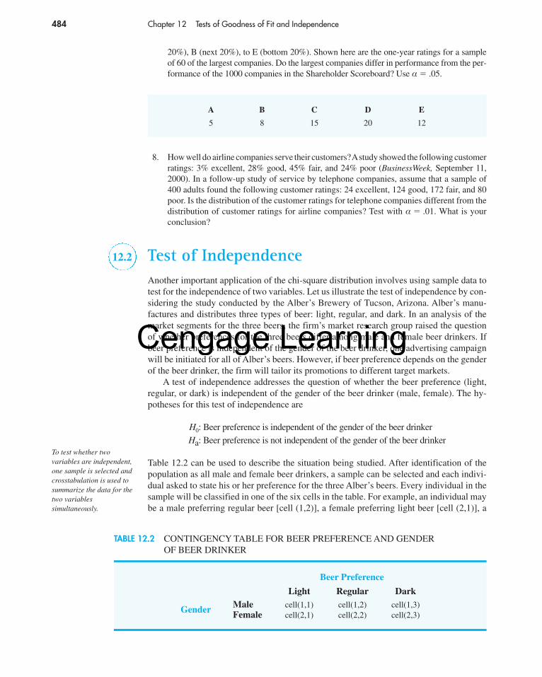
484 Chapter 12 Tests of Goodness of Fit and Independence
20%), B (next 20%), to E (bottom 20%). Shown here are the one-year ratings for a sampleof 60 of the largest companies. Do the largest companies differ in performance from the per-formance of the 1000 companies in the Shareholder Scoreboard? Use α � .05.
A B C D E
5 8 15 20 12
8. How well do airline companies serve their customers?Astudy showed the following customerratings: 3% excellent, 28% good, 45% fair, and 24% poor (BusinessWeek, September 11,2000). In a follow-up study of service by telephone companies, assume that a sample of400 adults found the following customer ratings: 24 excellent, 124 good, 172 fair, and 80poor. Is the distribution of the customer ratings for telephone companies different from thedistribution of customer ratings for airline companies? Test with α � .01. What is yourconclusion?
12.2 Test of IndependenceAnother important application of the chi-square distribution involves using sample data totest for the independence of two variables. Let us illustrate the test of independence by con-sidering the study conducted by the Alber’s Brewery of Tucson, Arizona. Alber’s manu-factures and distributes three types of beer: light, regular, and dark. In an analysis of themarket segments for the three beers, the firm’s market research group raised the questionof whether preferences for the three beers differ among male and female beer drinkers. Ifbeer preference is independent of the gender of the beer drinker, one advertising campaignwill be initiated for all of Alber’s beers. However, if beer preference depends on the genderof the beer drinker, the firm will tailor its promotions to different target markets.
A test of independence addresses the question of whether the beer preference (light, regular, or dark) is independent of the gender of the beer drinker (male, female). The hy-potheses for this test of independence are
Table 12.2 can be used to describe the situation being studied. After identification of thepopulation as all male and female beer drinkers, a sample can be selected and each indivi-dual asked to state his or her preference for the three Alber’s beers. Every individual in thesample will be classified in one of the six cells in the table. For example, an individual maybe a male preferring regular beer [cell (1,2)], a female preferring light beer [cell (2,1)], a
H0:
Ha: Beer preference is independent of the gender of the beer drinker
Beer preference is not independent of the gender of the beer drinker
Beer Preference
Light Regular DarkMale cell(1,1) cell(1,2) cell(1,3)Gender Female cell(2,1) cell(2,2) cell(2,3)
TABLE 12.2 CONTINGENCY TABLE FOR BEER PREFERENCE AND GENDER OF BEER DRINKER
To test whether twovariables are independent,one sample is selected andcrosstabulation is used tosummarize the data for thetwo variablessimultaneously.
56130_12_ch12_p476-507.qxd 2/22/08 10:51 PM Page 484
Cengage Learning

12.2 Test of Independence 485
female preferring dark beer [cell (2,3)], and so on. Because we have listed all possiblecombinations of beer preference and gender or, in other words, listed all possible contingen-cies, Table 12.2 is called a contingency table. The test of independence uses the contin-gency table format and for that reason is sometimes referred to as a contingency table test.
Suppose a simple random sample of 150 beer drinkers is selected. After tasting eachbeer, the individuals in the sample are asked to state their preference or first choice. Thecrosstabulation in Table 12.3 summarizes the responses for the study. As we see, the datafor the test of independence are collected in terms of counts or frequencies for each cell orcategory. Of the 150 individuals in the sample, 20 were men who favored light beer, 40 weremen who favored regular beer, 20 were men who favored dark beer, and so on.
The data in Table 12.3 are the observed frequencies for the six classes or categories.If we can determine the expected frequencies under the assumption of independence be-tween beer preference and gender of the beer drinker, we can use the chi-square distribu-tion to determine whether there is a significant difference between observed and expectedfrequencies.
Expected frequencies for the cells of the contingency table are based on the followingrationale. First we assume that the null hypothesis of independence between beer prefer-ence and gender of the beer drinker is true. Then we note that in the entire sample of 150 beer drinkers, a total of 50 prefer light beer, 70 prefer regular beer, and 30 prefer darkbeer. In terms of fractions we conclude that ⁵⁰⁄₁₅₀ � ¹⁄₃ of the beer drinkers prefer light beer,⁷⁰⁄₁₅₀ � ⁷⁄₁₅ prefer regular beer, and ³⁰⁄₁₅₀ � ¹⁄₅ prefer dark beer. If the independence assump-tion is valid, we argue that these fractions must be applicable to both male and female beerdrinkers. Thus, under the assumption of independence, we would expect the sample of 80 male beer drinkers to show that (¹⁄₃)80 � 26.67 prefer light beer, ( ⁷⁄₁₅)80 � 37.33 preferregular beer, and (¹⁄₅)80 � 16 prefer dark beer. Application of the same fractions to the 70 female beer drinkers provides the expected frequencies shown in Table 12.4.
Let eij denote the expected frequency for the contingency table category in row i andcolumn j. With this notation, let us reconsider the expected frequency calculation for males
Beer Preference
Light Regular Dark Total
Gender Male 20 40 20 80Female 30 30 10 70
Total 50 70 30 150
TABLE 12.3 SAMPLE RESULTS FOR BEER PREFERENCES OF MALE AND FEMALEBEER DRINKERS (OBSERVED FREQUENCIES)
Beer Preference
Light Regular Dark Total
Gender Male 26.67 37.33 16.00 80Female 23.33 32.67 14.00 70
Total 50.00 70.00 30.00 150
TABLE 12.4 EXPECTED FREQUENCIES IF BEER PREFERENCE IS INDEPENDENTOF THE GENDER OF THE BEER DRINKER
56130_12_ch12_p476-507.qxd 2/22/08 10:51 PM Page 485
Cengage Learning

486 Chapter 12 Tests of Goodness of Fit and Independence
(row i � 1) who prefer regular beer (column j � 2); that is, expected frequency e12. Follow-ing the preceding argument for the computation of expected frequencies, we can show that
This expression can be written slightly differently as
Note that 80 in the expression is the total number of males (row 1 total), 70 is the total num-ber of individuals preferring regular beer (column 2 total), and 150 is the total sample size.Hence, we see that
Generalization of the expression shows that the following formula provides the expectedfrequencies for a contingency table in the test of independence.
e12 �(Row 1 Total)(Column 2 Total)
Sample Size
e12 � (⁷�₁₅)80 � (⁷⁰�₁₅₀)80 �(80)(70)
150� 37.33
e12 � (⁷�₁₅)80 � 37.33
EXPECTED FREQUENCIES FOR CONTINGENCY TABLES UNDER THEASSUMPTION OF INDEPENDENCE
(12.2)eij �(Row i Total)(Column j Total)
Sample Size
TEST STATISTIC FOR INDEPENDENCE
(12.3)
where
fij � observed frequency for contingency table category in row i and column j
eij � expected frequency for contingency table category in row i and column jbased on the assumption of independence
Note: With n rows and m columns in the contingency table, the test statistic has a chi-square distribution with (n � 1)(m � 1) degrees of freedom provided that the ex-pected frequencies are 5 or more for all categories.
�2 � �i
�j
( fij � eij)2
eij
Using equation (12.2) for male beer drinkers who prefer dark beer, we find an expected frequency of e13 � (80)(30)/150 � 16.00, as shown in Table 12.4. Use equation (12.2) toverify the other expected frequencies shown in Table 12.4.
The test procedure for comparing the observed frequencies of Table 12.3 with theexpected frequencies of Table 12.4 is similar to the goodness of fit calculations made inSection 12.1. Specifically, the � 2 value based on the observed and expected frequencies iscomputed as follows.
56130_12_ch12_p476-507.qxd 2/22/08 10:51 PM Page 486
Cengage Learning
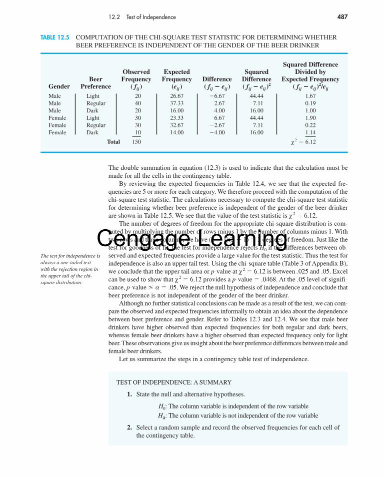
12.2 Test of Independence 487
The double summation in equation (12.3) is used to indicate that the calculation must bemade for all the cells in the contingency table.
By reviewing the expected frequencies in Table 12.4, we see that the expected fre-quencies are 5 or more for each category. We therefore proceed with the computation of thechi-square test statistic. The calculations necessary to compute the chi-square test statisticfor determining whether beer preference is independent of the gender of the beer drinkerare shown in Table 12.5. We see that the value of the test statistic is � 2 � 6.12.
The number of degrees of freedom for the appropriate chi-square distribution is com-puted by multiplying the number of rows minus 1 by the number of columns minus 1. Withtwo rows and three columns, we have (2 � 1)(3 � 1) � 2 degrees of freedom. Just like thetest for goodness of fit, the test for independence rejects H0 if the differences between ob-served and expected frequencies provide a large value for the test statistic. Thus the test forindependence is also an upper tail test. Using the chi-square table (Table 3 of Appendix B),we conclude that the upper tail area or p-value at � 2 � 6.12 is between .025 and .05. Excelcan be used to show that � 2 � 6.12 provides a p-value � .0468. At the .05 level of signifi-cance, p-value � α � .05. We reject the null hypothesis of independence and conclude thatbeer preference is not independent of the gender of the beer drinker.
Although no further statistical conclusions can be made as a result of the test, we can com-pare the observed and expected frequencies informally to obtain an idea about the dependencebetween beer preference and gender. Refer to Tables 12.3 and 12.4. We see that male beerdrinkers have higher observed than expected frequencies for both regular and dark beers,whereas female beer drinkers have a higher observed than expected frequency only for lightbeer. These observations give us insight about the beer preference differences between male andfemale beer drinkers.
Let us summarize the steps in a contingency table test of independence.
The test for independence isalways a one-tailed testwith the rejection region inthe upper tail of the chi-square distribution.
Squared DifferenceObserved Expected Squared Divided by
Beer Frequency Frequency Difference Difference Expected FrequencyGender Preference ( fij) (eij) ( fij � eij) ( fij � eij)
2 ( fij � eij)2/eij
Male Light 20 26.67 �6.67 44.44 1.67Male Regular 40 37.33 2.67 7.11 0.19Male Dark 20 16.00 4.00 16.00 1.00Female Light 30 23.33 6.67 44.44 1.90Female Regular 30 32.67 �2.67 7.11 0.22Female Dark 10 14.00 �4.00 16.00 1.14
Total 150 � 2 � 6.12
TABLE 12.5 COMPUTATION OF THE CHI-SQUARE TEST STATISTIC FOR DETERMINING WHETHERBEER PREFERENCE IS INDEPENDENT OF THE GENDER OF THE BEER DRINKER
TEST OF INDEPENDENCE: A SUMMARY
1. State the null and alternative hypotheses.
2. Select a random sample and record the observed frequencies for each cell ofthe contingency table.
H0:
Ha: The column variable is independent of the row variable
The column variable is not independent of the row variable
56130_12_ch12_p476-507.qxd 2/22/08 10:51 PM Page 487
Cengage Learning

A B C D E F G H I J1 Individual Gender Preference2 1 Female Light3 2 Female Regular Count of Individual Preference4 3 Male Regular Gender Light Regular Dark Grand Total5 4 Female Light Male 20 40 20 806 5 Female Light Female 30 30 10 707 6 Female Regular Grand Total 50 70 30 1508 7 Male Regular9 8 Female Dark Expected Frequencies
10 9 Female Regular Light Regular Dark11 10 Male Dark Male =F7*I5/I7 =G7*I5/I7 =H7*I5/I712 11 Male Regular Female =F7*I6/I7 =G7*I6/I7 =H7*I6/I713 12 Male Regular14 13 Female Regular p-value =CHITEST(F5:H6,F11:H12)15 14 Female Regular16 15 Male Light
149 148 Male Regular150 149 Female Light151 150 Female Regular152
488 Chapter 12 Tests of Goodness of Fit and Independence
Using Excel to Conduct a Test of IndependenceExcel can be used to conduct a test of independence for the Alber’s Brewery example. Re-fer to Figure 12.2 as we describe the tasks involved. The formula worksheet is in the back-ground; the value worksheet is in the foreground.
Enter Data: Column A is used to identify each of the 150 individuals in the study. ColumnB shows the gender and column C shows the beer preference (Light, Regular, or Dark) foreach individual.
Apply Tools: Using Excel’s PivotTable tool (see Section 2.4 for details regarding how touse this tool), we developed the crosstabulation shown in cells E3:I7. The values in cellsF5:H6 are the observed frequencies for the Alber’s Brewery study.
FIGURE 12.2 EXCEL WORKSHEET FOR THE ALBER’S BREWERY TEST OF INDEPENDENCE
3. Use equation (12.2) to compute the expected frequency for each cell.4. Use equation (12.3) to compute the value of the test statistic.5. Rejection rule:
where α is the level of significance, with n rows and m columns providing(n � 1)(m � 1) degrees of freedom.
p-value approach:
Critical value approach:
Reject H0 if p-value � αReject H0 if �
2 � � 2α
Note: Rows 17–148are hidden.
fileCDAlber’s
A B C D E F G H I J1 Individual Gender Preference2 1 Female Light3 2 Female Regular Count of Individual Preference4 3 Male Regular Gender Light Regular Dark Grand Total5 4 Female Light Male 20 40 20 806 5 Female Light Female 30 30 10 707 6 Female Regular Grand Total 50 70 30 1508 7 Male Regular9 8 Female Dark Expected Frequencies
10 9 Female Regular Light Regular Dark11 10 Male Dark Male 26.6667 37.3333 1612 11 Male Regular Female 23.3333 32.6667 1413 12 Male Regular14 13 Female Regular p-value 0.046815 14 Female Regular16 15 Male Light
149 148 Male Regular150 149 Female Light151 150 Female Regular152
56130_12_ch12_p476-507.qxd 2/22/08 10:51 PM Page 488
Cengage Learning
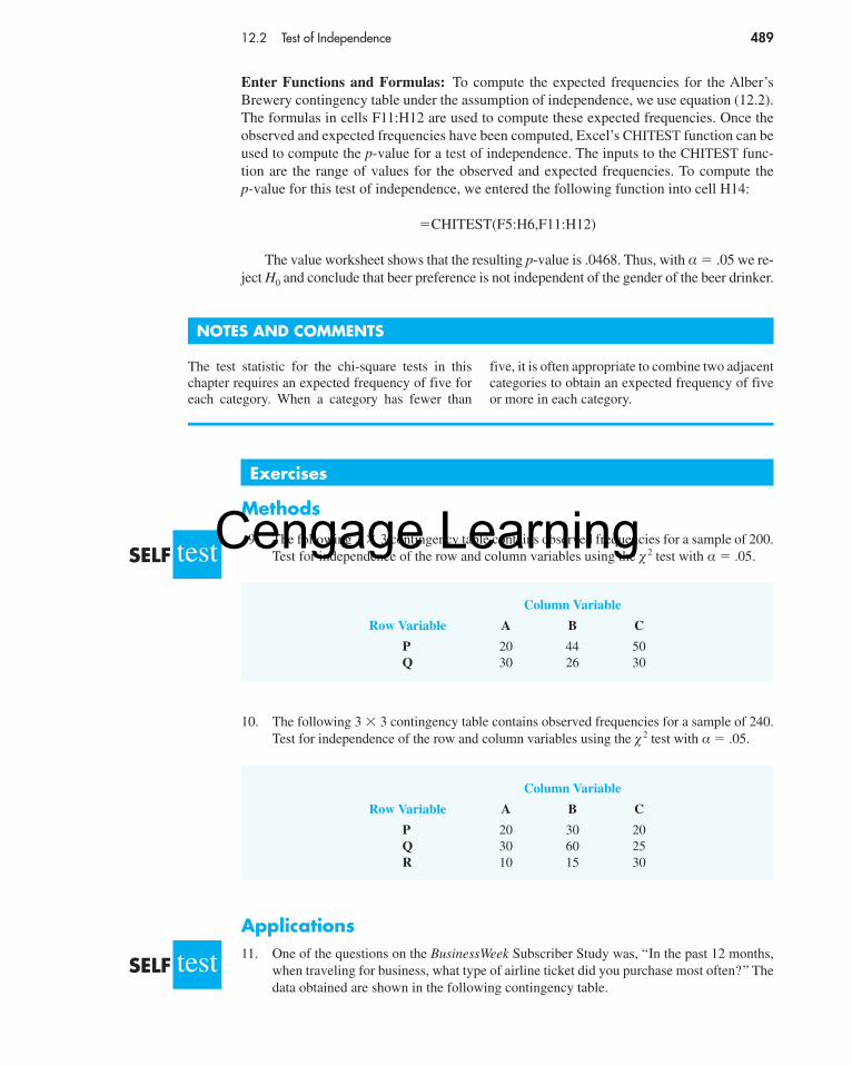
12.2 Test of Independence 489
Enter Functions and Formulas: To compute the expected frequencies for the Alber’sBrewery contingency table under the assumption of independence, we use equation (12.2).The formulas in cells F11:H12 are used to compute these expected frequencies. Once theobserved and expected frequencies have been computed, Excel’s CHITEST function can beused to compute the p-value for a test of independence. The inputs to the CHITEST func-tion are the range of values for the observed and expected frequencies. To compute the p-value for this test of independence, we entered the following function into cell H14:
The value worksheet shows that the resulting p-value is .0468. Thus, with α � .05 we re-ject H0 and conclude that beer preference is not independent of the gender of the beer drinker.
�CHITEST(F5:H6,F11:H12)
Exercises
Methods9. The following 2 � 3 contingency table contains observed frequencies for a sample of 200.
Test for independence of the row and column variables using the � 2 test with α � .05.
Column Variable
Row Variable A B C
P 20 30 20Q 30 60 25R 10 15 30
Column Variable
Row Variable A B C
P 20 44 50Q 30 26 30
testSELF
testSELF
NOTES AND COMMENTS
The test statistic for the chi-square tests in thischapter requires an expected frequency of five foreach category. When a category has fewer than
five, it is often appropriate to combine two adjacentcategories to obtain an expected frequency of fiveor more in each category.
10. The following 3 � 3 contingency table contains observed frequencies for a sample of 240.Test for independence of the row and column variables using the �2 test with α � .05.
Applications11. One of the questions on the BusinessWeek Subscriber Study was, “In the past 12 months,
when traveling for business, what type of airline ticket did you purchase most often?” Thedata obtained are shown in the following contingency table.
56130_12_ch12_p476-507.qxd 2/22/08 10:51 PM Page 489
Cengage Learning
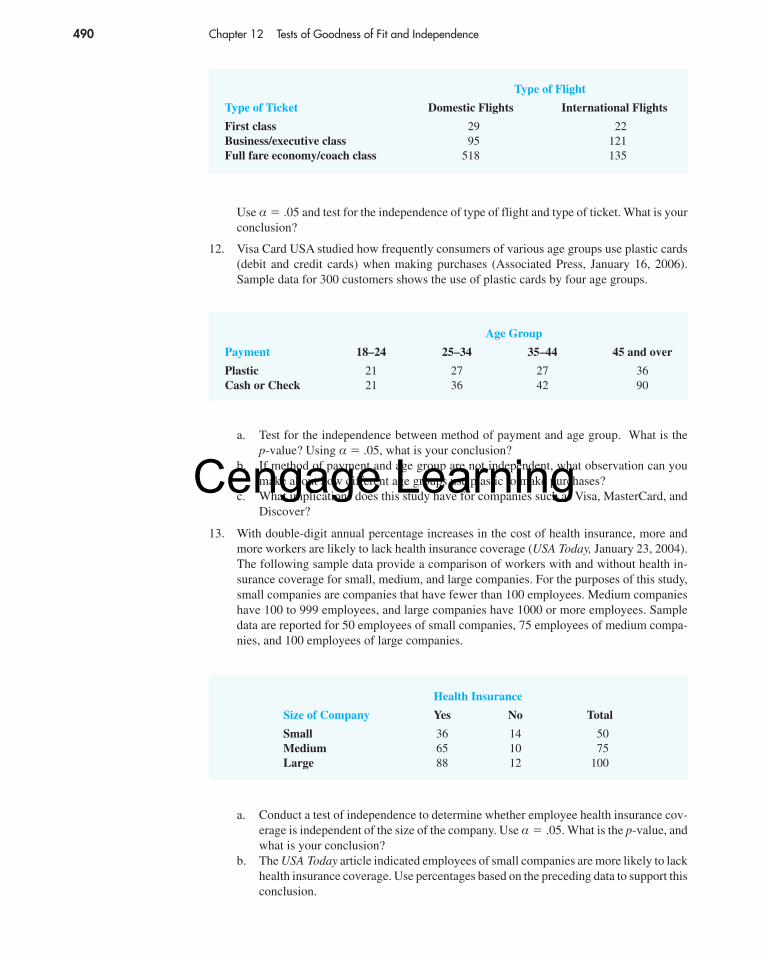
490 Chapter 12 Tests of Goodness of Fit and Independence
Use α � .05 and test for the independence of type of flight and type of ticket. What is yourconclusion?
12. Visa Card USA studied how frequently consumers of various age groups use plastic cards(debit and credit cards) when making purchases (Associated Press, January 16, 2006).Sample data for 300 customers shows the use of plastic cards by four age groups.
Type of Flight
Type of Ticket Domestic Flights International Flights
First class 29 22Business/executive class 95 121Full fare economy/coach class 518 135
Age Group
Payment 18–24 25–34 35–44 45 and over
Plastic 21 27 27 36Cash or Check 21 36 42 90
Health Insurance
Size of Company Yes No Total
Small 36 14 50Medium 65 10 75Large 88 12 100
a. Test for the independence between method of payment and age group. What is the p-value? Using α � .05, what is your conclusion?
b. If method of payment and age group are not independent, what observation can youmake about how different age groups use plastic to make purchases?
c. What implications does this study have for companies such as Visa, MasterCard, andDiscover?
13. With double-digit annual percentage increases in the cost of health insurance, more andmore workers are likely to lack health insurance coverage (USA Today, January 23, 2004).The following sample data provide a comparison of workers with and without health in-surance coverage for small, medium, and large companies. For the purposes of this study,small companies are companies that have fewer than 100 employees. Medium companieshave 100 to 999 employees, and large companies have 1000 or more employees. Sampledata are reported for 50 employees of small companies, 75 employees of medium compa-nies, and 100 employees of large companies.
a. Conduct a test of independence to determine whether employee health insurance cov-erage is independent of the size of the company. Use α � .05. What is the p-value, andwhat is your conclusion?
b. The USA Today article indicated employees of small companies are more likely to lackhealth insurance coverage. Use percentages based on the preceding data to support thisconclusion.
56130_12_ch12_p476-507.qxd 2/22/08 10:51 PM Page 490
Cengage Learning

12.2 Test of Independence 491
14. A State of Washington’s Public Interest Research Group (PIRG) study showed that 46% offull-time college students work 25 or more hours per week. The PIRG study provided dataon the effects of working on grades (USA Today, April 17, 2002). A sample of 200 studentsincluded 90 who worked 1 to 15 hours per week, 60 who worked 16 to 24 hours per week,and 50 who worked 25 to 34 hours per week. The sample number of students indicating theirwork had a positive effect, no effect, or a negative effect on grades is as follows.
Effect on Grades
Hours Worked per Week Positive None Negative Total
1–15 hours 26 50 14 9016–24 hours 16 27 17 6025–34 hours 11 19 20 50
Airline
Did It Fly? American Continental Delta United Total
Yes 48 69 68 25 210No 52 41 62 35 190
a. Conduct a test of independence to determine whether the effect on grades is indepen-dent of the hours worked per week. Use α � .05. What is the p-value, and what is yourconclusion?
b. Use row percentages to learn more about how working affects grades. What is yourconclusion?
15. FlightStats, Inc., collects data on the number of flights scheduled and the number of flightsflown at major airports throughout the United States. FlightStats data showed 56% offlights scheduled at Newark, La Guardia, and Kennedy airports were flown during a three-day snowstorm (The Wall Street Journal, February 21, 2006). All airlines say they alwaysoperate within set safety parameters—if conditions are too poor, they don’t fly. The fol-lowing data show a sample of 400 scheduled flights during the snowstorm.
Use the chi-square test of independence with a .05 level of significance to analyze the data.What is your conclusion? Do you have a preference for which airline you would choose tofly during similar snowstorm conditions? Explain.
16. Businesses are increasingly placing orders online. The Performance Measurement Groupcollected data on the rates of correctly filled electronic orders by industry (Investor’s Busi-ness Daily, May 8, 2000).Assume a sample of 700 electronic orders provided the followingresults.
a. Test a hypothesis to determine whether order fulfillment is independent of industry.Use α � .05. What is your conclusion?
b. Which industry has the highest percentage of correctly filled orders?
17. The National Sleep Foundation used a survey to determine whether hours of sleeping pernight are independent of age (Newsweek, January 19, 2004). The following table shows the
Industry
Order Pharmaceutical Consumer Computers Telecommunications
Correct 207 136 151 178Incorrect 3 4 9 12
56130_12_ch12_p476-507.qxd 2/22/08 10:51 PM Page 491
Cengage Learning

492 Chapter 12 Tests of Goodness of Fit and Independence
a. Conduct a test of independence to determine whether the hours of sleep on weeknightsare independent of age. Use α � .05. What is the p-value, and what is your conclusion?
b. What is your estimate of the percentage of people who sleep fewer than 6 hours, 6 to6.9 hours, 7 to 7.9 hours, and 8 or more hours on weeknights?
18. Samples taken in three cities, Anchorage, Atlanta, and Minneapolis, were used to learnabout the percentage of married couples with both the husband and the wife in the work-force (USA Today, January 15, 2006). Analyze the following data to see whether both thehusband and wife being in the workforce is independent of location. Use a .05 level of sig-nificance. What is your conclusion? What is the overall estimate of the percentage of mar-ried couples with both the husband and the wife in the workforce?
19. On a syndicated television show the two hosts often create the impression that theystrongly disagree about which movies are best. Each movie review is categorized as Pro(“thumbs up”), Con (“thumbs down”), or Mixed. The results of 160 movie ratings by thetwo hosts are shown here.
Hours of Sleep
Age Fewer than 6 6 to 6.9 7 to 7.9 8 or more Total
49 or younger 38 60 77 65 24050 or older 36 57 75 92 260
Location
In Workforce Anchorage Atlanta Minneapolis
Both 57 70 63Only One 33 50 90
Host B
Host A Con Mixed Pro
Con 24 8 13Mixed 8 13 11Pro 10 9 64
Use the chi-square test of independence with a .01 level of significance to analyze the data.What is your conclusion?
12.3 Goodness of Fit Test: Poisson and NormalDistributionsIn Section 12.1 we introduced the goodness of fit test for a multinomial population. In gen-eral, the goodness of fit test can be used with any hypothesized probability distribution. Inthis section we illustrate the goodness of fit test procedure for cases in which the popula-tion is hypothesized to have a Poisson or a normal distribution. As we shall see, the good-ness of fit test and the use of the chi-square distribution for the test follow the same generalprocedure used for the goodness of fit test in Section 12.1.
hours of sleep on weeknights for a sample of individuals age 49 and younger and for a sam-ple of individuals age 50 and older.
56130_12_ch12_p476-507.qxd 2/22/08 10:51 PM Page 492
Cengage Learning
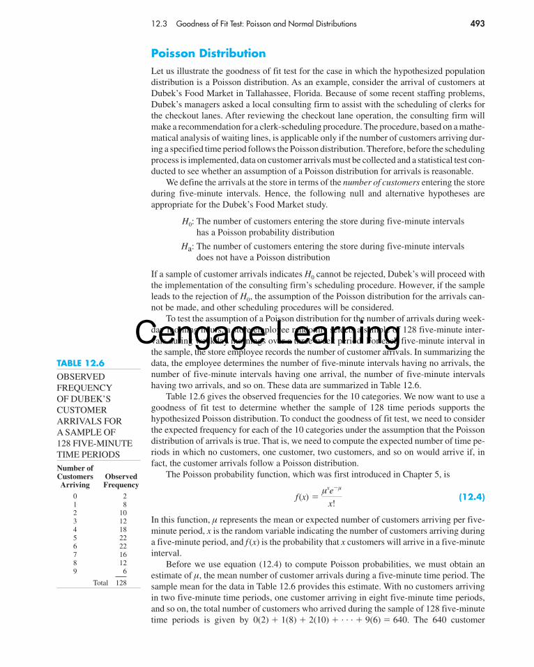
12.3 Goodness of Fit Test: Poisson and Normal Distributions 493
Poisson DistributionLet us illustrate the goodness of fit test for the case in which the hypothesized populationdistribution is a Poisson distribution. As an example, consider the arrival of customers atDubek’s Food Market in Tallahassee, Florida. Because of some recent staffing problems,Dubek’s managers asked a local consulting firm to assist with the scheduling of clerks forthe checkout lanes. After reviewing the checkout lane operation, the consulting firm willmake a recommendation for a clerk-scheduling procedure. The procedure, based on a mathe-matical analysis of waiting lines, is applicable only if the number of customers arriving dur-ing a specified time period follows the Poisson distribution. Therefore, before the schedulingprocess is implemented, data on customer arrivals must be collected and a statistical test con-ducted to see whether an assumption of a Poisson distribution for arrivals is reasonable.
We define the arrivals at the store in terms of the number of customers entering the storeduring five-minute intervals. Hence, the following null and alternative hypotheses areappropriate for the Dubek’s Food Market study.
H0: The number of customers entering the store during five-minute intervalshas a Poisson probability distribution
Ha: The number of customers entering the store during five-minute intervalsdoes not have a Poisson distribution
If a sample of customer arrivals indicates H0 cannot be rejected, Dubek’s will proceed withthe implementation of the consulting firm’s scheduling procedure. However, if the sampleleads to the rejection of H0, the assumption of the Poisson distribution for the arrivals can-not be made, and other scheduling procedures will be considered.
To test the assumption of a Poisson distribution for the number of arrivals during week-day morning hours, a store employee randomly selects a sample of 128 five-minute inter-vals during weekday mornings over a three-week period. For each five-minute interval inthe sample, the store employee records the number of customer arrivals. In summarizing thedata, the employee determines the number of five-minute intervals having no arrivals, thenumber of five-minute intervals having one arrival, the number of five-minute intervalshaving two arrivals, and so on. These data are summarized in Table 12.6.
Table 12.6 gives the observed frequencies for the 10 categories. We now want to use agoodness of fit test to determine whether the sample of 128 time periods supports thehypothesized Poisson distribution. To conduct the goodness of fit test, we need to considerthe expected frequency for each of the 10 categories under the assumption that the Poissondistribution of arrivals is true. That is, we need to compute the expected number of time pe-riods in which no customers, one customer, two customers, and so on would arrive if, infact, the customer arrivals follow a Poisson distribution.
The Poisson probability function, which was first introduced in Chapter 5, is
(12.4)
In this function, µ represents the mean or expected number of customers arriving per five-minute period, x is the random variable indicating the number of customers arriving duringa five-minute period, and f (x) is the probability that x customers will arrive in a five-minuteinterval.
Before we use equation (12.4) to compute Poisson probabilities, we must obtain anestimate of µ, the mean number of customer arrivals during a five-minute time period. The sample mean for the data in Table 12.6 provides this estimate. With no customers arrivingin two five-minute time periods, one customer arriving in eight five-minute time periods,and so on, the total number of customers who arrived during the sample of 128 five-minutetime periods is given by 0(2) � 1(8) � 2(10) � . . . � 9(6) � 640. The 640 customer
f(x) �µxe�µ
x!
TABLE 12.6OBSERVEDFREQUENCYOF DUBEK’SCUSTOMERARRIVALS FOR A SAMPLE OF 128 FIVE-MINUTE TIME PERIODS
Number ofCustomers ObservedArriving Frequency
0 21 82 103 124 185 226 227 168 129 6
Total 128
56130_12_ch12_p476-507.qxd 2/22/08 10:51 PM Page 493
Cengage Learning
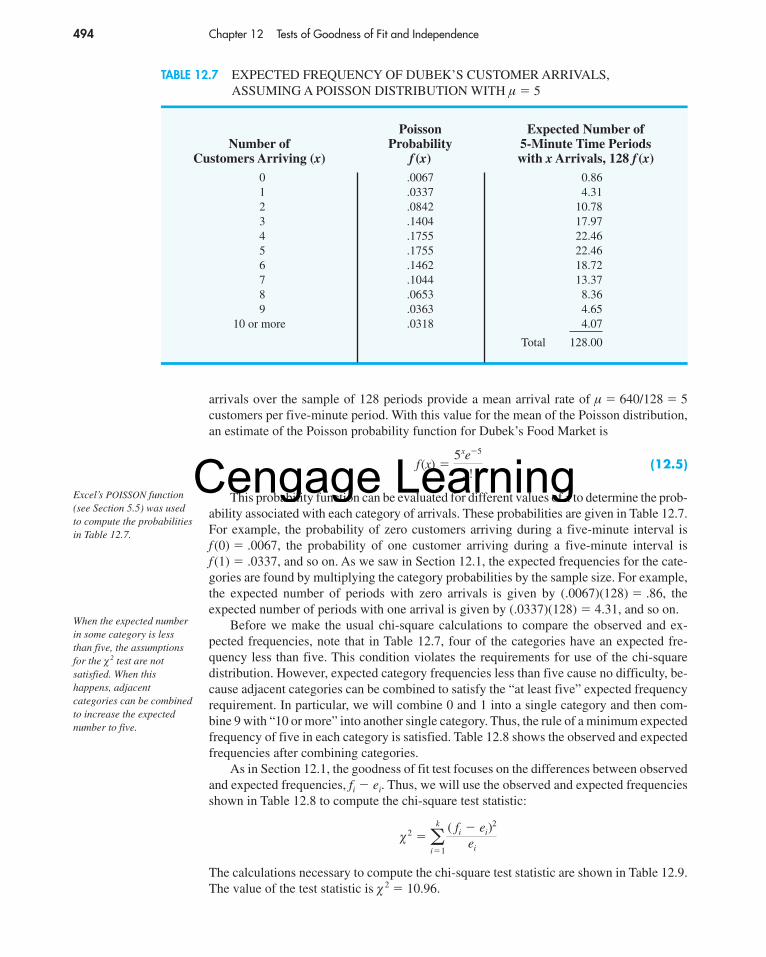
494 Chapter 12 Tests of Goodness of Fit and Independence
arrivals over the sample of 128 periods provide a mean arrival rate of µ � 640/128 � 5customers per five-minute period. With this value for the mean of the Poisson distribution,an estimate of the Poisson probability function for Dubek’s Food Market is
(12.5)
This probability function can be evaluated for different values of x to determine the prob-ability associated with each category of arrivals. These probabilities are given in Table 12.7.For example, the probability of zero customers arriving during a five-minute interval isf (0) � .0067, the probability of one customer arriving during a five-minute interval isf (1) � .0337, and so on. As we saw in Section 12.1, the expected frequencies for the cate-gories are found by multiplying the category probabilities by the sample size. For example,the expected number of periods with zero arrivals is given by (.0067)(128) � .86, theexpected number of periods with one arrival is given by (.0337)(128) � 4.31, and so on.
Before we make the usual chi-square calculations to compare the observed and ex-pected frequencies, note that in Table 12.7, four of the categories have an expected fre-quency less than five. This condition violates the requirements for use of the chi-squaredistribution. However, expected category frequencies less than five cause no difficulty, be-cause adjacent categories can be combined to satisfy the “at least five” expected frequencyrequirement. In particular, we will combine 0 and 1 into a single category and then com-bine 9 with “10 or more” into another single category. Thus, the rule of a minimum expectedfrequency of five in each category is satisfied. Table 12.8 shows the observed and expectedfrequencies after combining categories.
As in Section 12.1, the goodness of fit test focuses on the differences between observedand expected frequencies, fi � ei. Thus, we will use the observed and expected frequenciesshown in Table 12.8 to compute the chi-square test statistic:
The calculations necessary to compute the chi-square test statistic are shown in Table 12.9.The value of the test statistic is � 2 � 10.96.
�2 � �k
i�1
( fi � ei)
2
ei
f(x) �5xe�5
x!
Poisson Expected Number ofNumber of Probability 5-Minute Time Periods
Customers Arriving (x) f (x) with x Arrivals, 128 f (x)0 .0067 0.861 .0337 4.312 .0842 10.783 .1404 17.974 .1755 22.465 .1755 22.466 .1462 18.727 .1044 13.378 .0653 8.369 .0363 4.65
10 or more .0318 4.07
Total 128.00
TABLE 12.7 EXPECTED FREQUENCY OF DUBEK’S CUSTOMER ARRIVALS, ASSUMING A POISSON DISTRIBUTION WITH µ � 5
Excel’s POISSON function(see Section 5.5) was usedto compute the probabilitiesin Table 12.7.
When the expected numberin some category is lessthan five, the assumptionsfor the � 2 test are notsatisfied. When thishappens, adjacentcategories can be combinedto increase the expectednumber to five.
56130_12_ch12_p476-507.qxd 2/22/08 10:51 PM Page 494
Cengage Learning
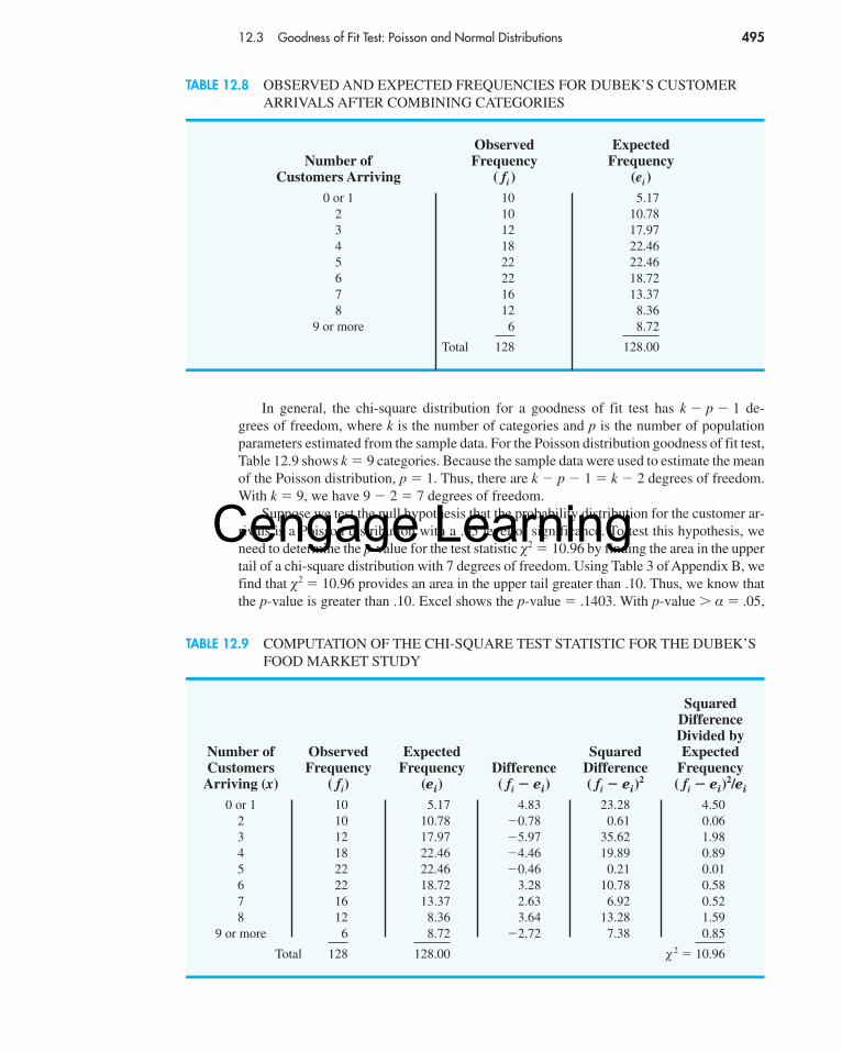
12.3 Goodness of Fit Test: Poisson and Normal Distributions 495
In general, the chi-square distribution for a goodness of fit test has k � p � 1 de-grees of freedom, where k is the number of categories and p is the number of populationparameters estimated from the sample data. For the Poisson distribution goodness of fit test,Table 12.9 shows k � 9 categories. Because the sample data were used to estimate the meanof the Poisson distribution, p � 1. Thus, there are k � p � 1 � k � 2 degrees of freedom.With k � 9, we have 9 � 2 � 7 degrees of freedom.
Suppose we test the null hypothesis that the probability distribution for the customer ar-rivals is a Poisson distribution with a .05 level of significance. To test this hypothesis, weneed to determine the p-value for the test statistic �2 � 10.96 by finding the area in the uppertail of a chi-square distribution with 7 degrees of freedom. Using Table 3 of Appendix B, wefind that �2 � 10.96 provides an area in the upper tail greater than .10. Thus, we know thatthe p-value is greater than .10. Excel shows the p-value � .1403. With p-value � α � .05,
SquaredDifferenceDivided by
Number of Observed Expected Squared ExpectedCustomers Frequency Frequency Difference Difference Frequency
Arriving (x) ( fi) (ei) ( fi � ei) ( fi � ei)2 ( fi � ei)
2/ei
0 or 1 10 5.17 4.83 23.28 4.502 10 10.78 �0.78 0.61 0.063 12 17.97 �5.97 35.62 1.984 18 22.46 �4.46 19.89 0.895 22 22.46 �0.46 0.21 0.016 22 18.72 3.28 10.78 0.587 16 13.37 2.63 6.92 0.528 12 8.36 3.64 13.28 1.59
9 or more 6 8.72 �2.72 7.38 0.85
Total 128 128.00 � 2 � 10.96
TABLE 12.9 COMPUTATION OF THE CHI-SQUARE TEST STATISTIC FOR THE DUBEK’SFOOD MARKET STUDY
Observed ExpectedNumber of Frequency Frequency
Customers Arriving ( fi) (ei)0 or 1 10 5.17
2 10 10.783 12 17.974 18 22.465 22 22.466 22 18.727 16 13.378 12 8.36
9 or more 6 8.72
Total 128 128.00
TABLE 12.8 OBSERVED AND EXPECTED FREQUENCIES FOR DUBEK’S CUSTOMERARRIVALS AFTER COMBINING CATEGORIES
56130_12_ch12_p476-507.qxd 2/22/08 10:51 PM Page 495
Cengage Learning

496 Chapter 12 Tests of Goodness of Fit and Independence
POISSON DISTRIBUTION GOODNESS OF FIT TEST: A SUMMARY
1. State the null and alternative hypotheses.
2. Select a random sample anda. Record the observed frequency fi for each value of the Poisson random
variable.b. Compute the mean number of occurrences µ.
3. Compute the expected frequency of occurrences ei for each value of the Pois-son random variable. Multiply the sample size by the Poisson probability ofoccurrence for each value of the Poisson random variable. If there are fewerthan five expected occurrences for some values, combine adjacent values andreduce the number of categories as necessary.
4. Compute the value of the test statistic.
5. Rejection rule:
where α is the level of significance and there are k – 2 degrees of freedom.
p-value approach:
Critical value approach:
Reject H0 if p-value � αReject H0 if �
2 � � 2α
� 2 � �k
i�1
( fi � ei)
2
ei
H0:
Ha: The population has a Poisson distribution
The population does not have a Poisson distribution
Using Excel to Conduct a Goodness of Fit TestIn Section 12.1 we showed how Excel could be used to conduct a multinomial goodness offit test. A similar approach can be used to conduct a Poisson distribution goodness of fit test.Refer to Figure 12.1 as we discuss the approach. The nine categories corresponding to thenumber of arrivals in Table 12.9 would replace the three companies listed in column D ofthe worksheet, and the probability associated with each category of arrivals would be com-puted in column E using Excel’s POISSON function. The only data are the observed fre-quencies, which would be typed directly into column F. The expected frequencies would becomputed in column G by multiplying the probabilities in column E by the sample size. Theformulas in columns H, I, and J used to compute the � 2 test statistic using equation (12.1)are the same as in the worksheet in Figure 12.1. The chi-square value obtained is 10.9628.The only other change necessary is that the cell formula for the degrees of freedom must bechanged from k � 1 for the multinomial goodness of fit test to k � 2 for the Poisson distri-bution goodness of fit test. With these changes, the p-value for the test is computed usingExcel’s CHIDIST function as we described in Section 12.1. For the Dubek’s Food Marketgoodness of fit test, CHIDIST(10.9628,7) provides a p-value of .1403. With .1403 � α � .05,we cannot reject the null hypothesis that the number of customers entering the store duringfive-minute intervals has a Poisson distribution.
we cannot reject H0. Hence, the assumption of a Poisson probability distribution for week-day morning customer arrivals cannot be rejected. As a result, Dubek’s management mayproceed with the consulting firm’s scheduling procedure for weekday mornings.
56130_12_ch12_p476-507.qxd 2/22/08 10:51 PM Page 496
Cengage Learning
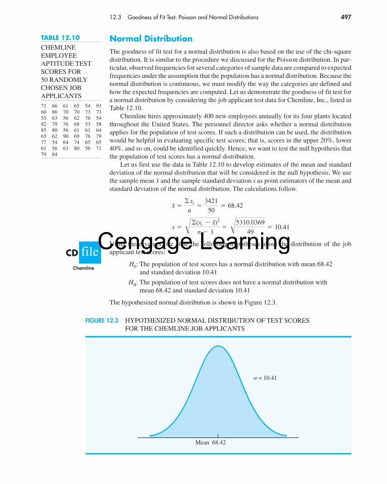
12.3 Goodness of Fit Test: Poisson and Normal Distributions 497
Normal DistributionThe goodness of fit test for a normal distribution is also based on the use of the chi-squaredistribution. It is similar to the procedure we discussed for the Poisson distribution. In par-ticular, observed frequencies for several categories of sample data are compared to expectedfrequencies under the assumption that the population has a normal distribution. Because thenormal distribution is continuous, we must modify the way the categories are defined andhow the expected frequencies are computed. Let us demonstrate the goodness of fit test fora normal distribution by considering the job applicant test data for Chemline, Inc., listed inTable 12.10.
Chemline hires approximately 400 new employees annually for its four plants locatedthroughout the United States. The personnel director asks whether a normal distributionapplies for the population of test scores. If such a distribution can be used, the distributionwould be helpful in evaluating specific test scores; that is, scores in the upper 20%, lower40%, and so on, could be identified quickly. Hence, we want to test the null hypothesis thatthe population of test scores has a normal distribution.
Let us first use the data in Table 12.10 to develop estimates of the mean and standarddeviation of the normal distribution that will be considered in the null hypothesis. We usethe sample mean and the sample standard deviation s as point estimators of the mean andstandard deviation of the normal distribution. The calculations follow.
Using these values, we state the following hypotheses about the distribution of the jobapplicant test scores:
H0: The population of test scores has a normal distribution with mean 68.42and standard deviation 10.41
Ha: The population of test scores does not have a normal distribution with mean 68.42 and standard deviation 10.41
The hypothesized normal distribution is shown in Figure 12.3.
s � � �(xi � x̄)2
n � 1� �5310.0369
49� 10.41
x̄ �� xi
n�
3421
50� 68.42
x̄
fileCDChemline
Mean 68.42
σ = 10.41
FIGURE 12.3 HYPOTHESIZED NORMAL DISTRIBUTION OF TEST SCORES FOR THE CHEMLINE JOB APPLICANTS
TABLE 12.10CHEMLINEEMPLOYEEAPTITUDE TESTSCORES FOR 50 RANDOMLYCHOSEN JOBAPPLICANTS
71 66 61 65 54 9360 86 70 70 73 7355 63 56 62 76 5482 79 76 68 53 5885 80 56 61 61 6465 62 90 69 76 7977 54 64 74 65 6561 56 63 80 56 7179 84
56130_12_ch12_p476-507.qxd 2/22/08 10:51 PM Page 497
Cengage Learning
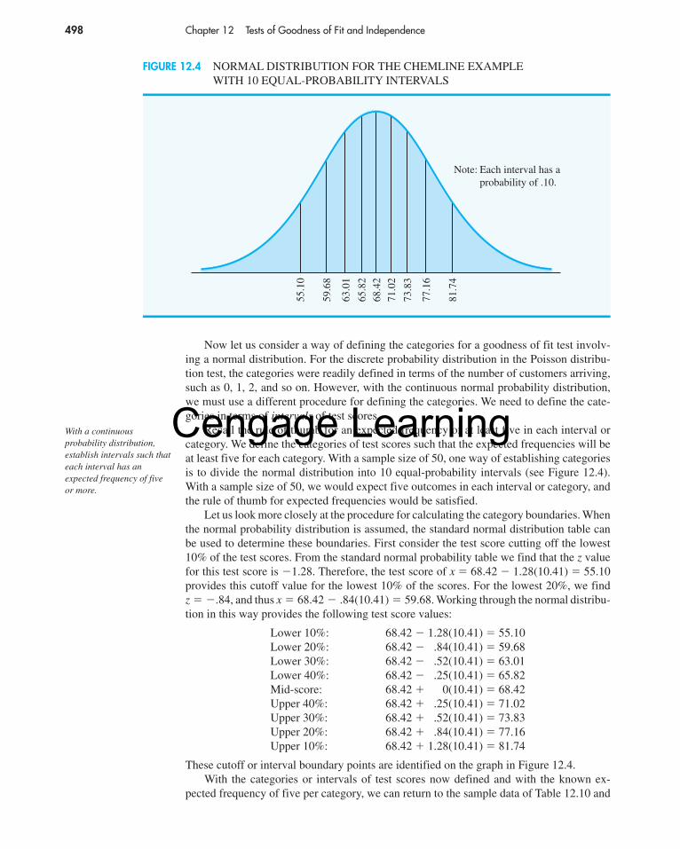
498 Chapter 12 Tests of Goodness of Fit and Independence
Now let us consider a way of defining the categories for a goodness of fit test involv-ing a normal distribution. For the discrete probability distribution in the Poisson distribu-tion test, the categories were readily defined in terms of the number of customers arriving,such as 0, 1, 2, and so on. However, with the continuous normal probability distribution,we must use a different procedure for defining the categories. We need to define the cate-gories in terms of intervals of test scores.
Recall the rule of thumb for an expected frequency of at least five in each interval orcategory. We define the categories of test scores such that the expected frequencies will beat least five for each category. With a sample size of 50, one way of establishing categoriesis to divide the normal distribution into 10 equal-probability intervals (see Figure 12.4).With a sample size of 50, we would expect five outcomes in each interval or category, andthe rule of thumb for expected frequencies would be satisfied.
Let us look more closely at the procedure for calculating the category boundaries. Whenthe normal probability distribution is assumed, the standard normal distribution table canbe used to determine these boundaries. First consider the test score cutting off the lowest10% of the test scores. From the standard normal probability table we find that the z valuefor this test score is �1.28. Therefore, the test score of x � 68.42 � 1.28(10.41) � 55.10provides this cutoff value for the lowest 10% of the scores. For the lowest 20%, we findz � �.84, and thus x � 68.42 � .84(10.41) � 59.68. Working through the normal distribu-tion in this way provides the following test score values:
Lower 10%: 68.42 � 1.28(10.41) � 55.10Lower 20%: 68.42 � .84(10.41) � 59.68Lower 30%: 68.42 � .52(10.41) � 63.01Lower 40%: 68.42 � .25(10.41) � 65.82Mid-score: 68.42 � 0(10.41) � 68.42Upper 40%: 68.42 � .25(10.41) � 71.02Upper 30%: 68.42 � .52(10.41) � 73.83Upper 20%: 68.42 � .84(10.41) � 77.16Upper 10%: 68.42 � 1.28(10.41) � 81.74
These cutoff or interval boundary points are identified on the graph in Figure 12.4.With the categories or intervals of test scores now defined and with the known ex-
pected frequency of five per category, we can return to the sample data of Table 12.10 and
Note:
55.1
0
59.6
8
63.0
1
65.8
2
68.4
2
71.0
2
73.8
3
77.1
6
81.7
4
Each interval has aprobability of .10.
FIGURE 12.4 NORMAL DISTRIBUTION FOR THE CHEMLINE EXAMPLE WITH 10 EQUAL-PROBABILITY INTERVALS
With a continuousprobability distribution,establish intervals such thateach interval has anexpected frequency of fiveor more.
56130_12_ch12_p476-507.qxd 2/22/08 10:51 PM Page 498
Cengage Learning

12.3 Goodness of Fit Test: Poisson and Normal Distributions 499
determine the observed frequencies for the categories. Doing so provides the results inTable 12.11.
With the results in Table 12.11, the goodness of fit calculations proceed exactly as be-fore. Namely, we compare the observed and expected results by computing a � 2 value. Thecomputations necessary to compute the chi-square test statistic are shown in Table 12.12.We see that the value of the test statistic is � 2 � 7.2.
To determine whether the computed �2 value of 7.2 is large enough to reject H0, we needto refer to the appropriate chi-square distribution tables. Using the rule for computing the num-ber of degrees of freedom for the goodness of fit test, we have k � p � 1 � 10 � 2 � 1 � 7degrees of freedom based on k � 10 categories and p � 2 parameters (mean and standarddeviation) estimated from the sample data.
Observed ExpectedFrequency Frequency
Test Score Interval ( fi) (ei)Less than 55.10 5 555.10 to 59.68 5 559.68 to 63.01 9 563.01 to 65.82 6 565.82 to 68.42 2 568.42 to 71.02 5 571.02 to 73.83 2 573.83 to 77.16 5 577.16 to 81.74 5 581.74 and Over 6 5
Total 50 50
TABLE 12.11 OBSERVED AND EXPECTED FREQUENCIES FOR CHEMLINE JOBAPPLICANT TEST SCORES
SquaredDifferenceDivided by
Observed Expected Squared ExpectedTest Score Frequency Frequency Difference Difference FrequencyInterval ( fi) (ei) ( fi � ei) ( fi � ei)
2 ( fi � ei)2/ei
Less than 55.10 5 5 0 0 0.055.10 to 59.68 5 5 0 0 0.059.68 to 63.01 9 5 4 16 3.263.01 to 65.82 6 5 1 1 0.265.82 to 68.42 2 5 �3 9 1.868.42 to 71.02 5 5 0 0 0.071.02 to 73.83 2 5 �3 9 1.873.83 to 77.16 5 5 0 0 0.077.16 to 81.74 5 5 0 0 0.081.74 and Over 6 5 1 1 0.2
Total 50 50 � 2 � 7.2
TABLE 12.12 COMPUTATION OF THE CHI-SQUARE TEST STATISTIC FOR THE CHEMLINE JOB APPLICANT EXAMPLE
Estimating µ and σ, the twoparameters of the normaldistribution, will cause aloss of two degrees offreedom in the � 2 test.
56130_12_ch12_p476-507.qxd 2/22/08 10:51 PM Page 499
Cengage Learning
500 Chapter 12 Tests of Goodness of Fit and Independence
NORMAL DISTRIBUTION GOODNESS OF FIT TEST: A SUMMARY
1. State the null and alternative hypotheses.
2. Select a random sample anda. Compute the sample mean and sample standard deviation.b. Define intervals of values so that the expected frequency is at least five for
each interval. Using equal probability intervals is a good approach.c. Record the observed frequency of data values fi in each interval defined.
3. Compute the expected number of occurrences ei for each interval of valuesdefined in step 2(b). Multiply the sample size by the probability of a normalrandom variable being in the interval.
4. Compute the value of the test statistic.
5. Rejection rule:
where α is the level of significance and there are k – 3 degrees of freedom.
p-value approach:
Critical value approach:
Reject H0 if p-value � αReject H0 if �
2 � � 2α
� 2 � �k
i�1
( fi � ei)
2
ei
H0:
Ha: The population has a normal distribution
The population does not have a normal distribution
Suppose that we test the null hypothesis that the distribution for the test scores is anormal distribution with a .10 level of significance. To test this hypothesis, we need todetermine the p-value for the test statistic � 2 � 7.2 by finding the area in the upper tail ofa chi-square distribution with 7 degrees of freedom. Using Table 3 of Appendix B, we findthat � 2 � 7.2 provides an area in the upper tail greater than .10. Thus, we know that the p-value is greater than .10. Using Excel the exact p-value � .4084. With the p-value �α � .10, the hypothesis that the probability distribution for the Chemline job applicant testscores is a normal distribution cannot be rejected. The normal distribution may be appliedto assist in the interpretation of test scores. A summary of the goodness fit test for a normaldistribution follows.
Using Excel to Conduct a Goodness of Fit TestIn Section 12.1 we showed how Excel could be used to conduct a multinomial goodnessof fit test. A similar approach can be used to conduct a normal distribution goodness of fit test. Refer to Figure 12.1 as we discuss the approach. The 10 categories correspond-ing to the test score intervals would replace the three companies listed in column D of the worksheet. The only data would be the observed and expected frequencies; they wouldbe typed directly into columns F and G. The formulas in columns H, I, and J used to com-pute the � 2 test statistic using equation (12.1) are the same as in the worksheet in Fig-ure 12.1. The only other change necessary is that the cell formula for the degrees of free-dom must be changed from k � 1 for the multinomial goodness of fit test to k � 3 for thenormal distribution goodness of fit test. With these changes, the p-value for the test iscomputed using Excel’s CHIDIST function as we described in Section 12.1. For the Chem-line goodness of fit test CHIDIST(7.2,7) provides a p-value of .4084. With .4084 � α �.10, we cannot reject the null hypothesis that the Chemline applicant test scores follow anormal distribution.
56130_12_ch12_p476-507.qxd 2/22/08 10:51 PM Page 500
Cengage Learning

12.3 Goodness of Fit Test: Poisson and Normal Distributions 501
Exercises
Methods20. Data on the number of occurrences per time period and observed frequencies follow. Use
α � .05 and the goodness of fit test to see whether the data fit a Poisson distribution.
21. The following data are believed to have come from a normal distribution. Use the good-ness of fit test and α � .05 to test this claim.
17 23 22 24 19 23 18 22 20 13 11 21 18 20 2121 18 15 24 23 23 43 29 27 26 30 28 33 23 29
Applications22. The number of automobile accidents per day in a particular city is believed to have a Pois-
son distribution. A sample of 80 days during the past year gives the following data. Dothese data support the belief that the number of accidents per day has a Poisson distribu-tion? Use α � .05.
Observed FrequencyNumber of Accidents (days)
0 341 252 113 74 3
Number of IncomingPhone Calls During
a One-Minute Interval Observed Frequency
0 151 312 203 154 135 46 2
Total 100
23. The number of incoming phone calls at a company switchboard during one-minute inter-vals is believed to have a Poisson distribution. Use α � .10 and the following data to testthe assumption that the incoming phone calls follow a Poisson distribution.
Number of Occurrences Observed Frequency
0 391 302 303 184 3
testSELF
testSELF
56130_12_ch12_p476-507.qxd 2/22/08 10:51 PM Page 501
Cengage Learning
502 Chapter 12 Tests of Goodness of Fit and Independence
24. The weekly demand for a product is believed to be normally distributed. Use a goodnessof fit test and the following data to test this assumption. Use α � .10. The sample mean is24.5 and the sample standard deviation is 3.
18 20 22 27 2225 22 27 25 2426 23 20 24 2627 25 19 21 2526 25 31 29 2525 28 26 28 24
25. Use α � .01 and conduct a goodness of fit test to see whether the following sample ap-pears to have been selected from a normal distribution.
55 86 94 58 55 95 55 52 69 95 90 65 87 50 5655 57 98 58 79 92 62 59 88 65
After you complete the goodness of fit calculations, construct a histogram of the data. Doesthe histogram representation support the conclusion reached with the goodness of fit test?(Note: and s � 17.)
Summary
In this chapter we introduced the goodness of fit test and the test of independence, both of which are based on the use of the chi-square distribution. The purpose of the good-ness of fit test is to determine whether a hypothesized probability distribution can be used as a model for a particular population of interest. The computations for conductingthe goodness of fit test involve comparing observed frequencies from a sample withexpected frequencies when the hypothesized probability distribution is assumed true. Achi-square distribution is used to determine whether the differences between observed and expected frequencies are large enough to reject the hypothesized probability dis-tribution. We illustrated the goodness of fit test for multinomial, Poisson, and normaldistributions.
A test of independence for two variables is an extension of the methodology employedin the goodness of fit test for a multinomial population. A contingency table is used to de-termine the observed and expected frequencies. Then a chi-square value is computed. Largechi-square values, caused by large differences between observed and expected frequencies,lead to the rejection of the null hypothesis of independence.
Glossary
Multinomial population A population in which each element is assigned to one and onlyone of several categories. The multinomial distribution extends the binomial distributionfrom two to three or more outcomes.Goodness of fit test A statistical test conducted to determine whether to reject a hypothe-sized probability distribution for a population.Contingency table A table used to summarize observed and expected frequencies for a testof independence.
x̄ � 71
56130_12_ch12_p476-507.qxd 2/22/08 10:51 PM Page 502
Cengage Learning

Supplementary Exercises 503
Key Formulas
Test Statistic for Goodness of Fit
(12.1)
Expected Frequencies for Contingency Tables Under the Assumption of Independence
(12.2)
Test Statistic for Independence
(12.3)
Supplementary Exercises
26. In setting sales quotas, the marketing manager makes the assumption that order potentialsare the same for each of four sales territories. A sample of 200 sales follows. Should themanager’s assumption be rejected? Use α � .05.
� 2 � �i
�j
( fij � eij)2
eij
eij �(Row i Total)(Column j Total)
Sample Size
� 2 � �k
i�1
( fi � ei
)2
ei
Sales Territories
I II III IV
60 45 59 36
Safety Rating Frequency
Very safe 48Somewhat safe 323Not very safe 79Not at all safe 16Not sure 63
Total 529
27. Seven percent of mutual fund investors rate corporate stocks “very safe,” 58% rate them“somewhat safe,” 24% rate them “not very safe,” 4% rate them “not at all safe,” and 7%are “not sure.” A BusinessWeek/Harris poll asked 529 mutual fund investors how theywould rate corporate bonds on safety. The responses are as follows.
Do mutual fund investors’ attitudes toward corporate bonds differ from their attitudes to-ward corporate stocks? Support your conclusion with a statistical test. Use α � .01.
28. Since 2000, the Toyota Camry, Honda Accord, and Ford Taurus have been the three best-selling passenger cars in the United States. Based on the 2003 sales data, the market sharesamong the top three are as follows: Toyota Camry 37%, Honda Accord 34%, and Ford Tau-rus 29% (The World Almanac, 2004). Assume a sample of 1200 sales of passenger carsduring the first quarter of 2004 shows the following.
56130_12_ch12_p476-507.qxd 2/22/08 10:51 PM Page 503
Cengage Learning

504 Chapter 12 Tests of Goodness of Fit and Independence
Can these data be used to conclude that the market shares among the top three passengercars have changed during the first quarter of 2004? What is the p-value? Use a .05 level ofsignificance. What is your conclusion?
29. A regional transit authority is concerned about the number of riders on one of its bus routes.In setting up the route, the assumption is that the number of riders is the same on every dayfrom Monday through Friday. Using the following data, test with α � .05 to determinewhether the transit authority’s assumption is correct.
30. The results of Computerworld’s Annual Job Satisfaction Survey showed that 28% ofinformation systems (IS) managers are very satisfied with their job, 46% are somewhatsatisfied, 12% are neither satisfied nor dissatisfied, 10% are somewhat dissatisfied, and 4%are very dissatisfied. Suppose that a sample of 500 computer programmers yielded thefollowing results.
Use α � .05 and test to determine whether the job satisfaction for computer programmersis different from the job satisfaction for IS managers.
31. A sample of parts provided the following contingency table data on part quality by pro-duction shift.
Number ofDay Riders
Monday 13Tuesday 16Wednesday 28Thursday 17Friday 16
Number ofCategory Respondents
Very satisfied 105Somewhat satisfied 235Neither 55Somewhat dissatisfied 90Very dissatisfied 15
Number NumberShift Good Defective
First 368 32Second 285 15Third 176 24
Use α � .05 and test the hypothesis that part quality is independent of the production shift.What is your conclusion?
Passenger Car Units Sold
Toyota Camry 480Honda Accord 390Ford Taurus 330
56130_12_ch12_p476-507.qxd 2/22/08 10:51 PM Page 504
Cengage Learning
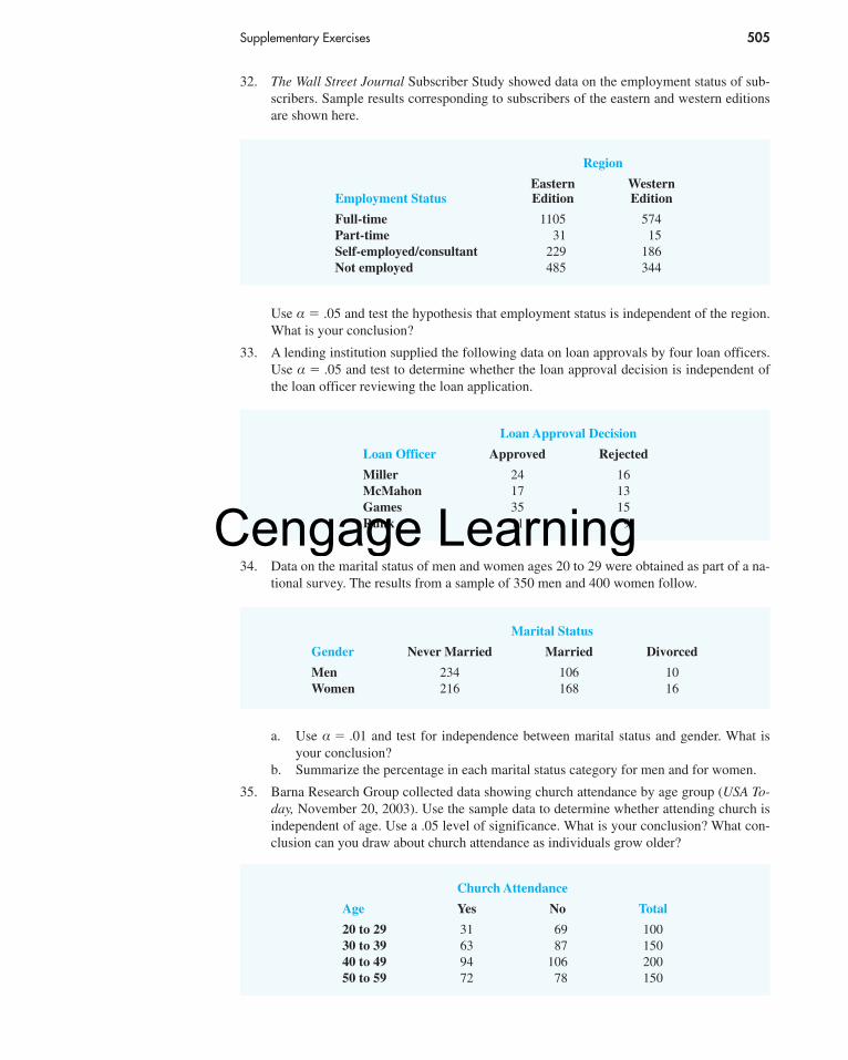
Supplementary Exercises 505
32. The Wall Street Journal Subscriber Study showed data on the employment status of sub-scribers. Sample results corresponding to subscribers of the eastern and western editionsare shown here.
Use α � .05 and test the hypothesis that employment status is independent of the region.What is your conclusion?
33. A lending institution supplied the following data on loan approvals by four loan officers.Use α � .05 and test to determine whether the loan approval decision is independent ofthe loan officer reviewing the loan application.
34. Data on the marital status of men and women ages 20 to 29 were obtained as part of a na-tional survey. The results from a sample of 350 men and 400 women follow.
Loan Approval Decision
Loan Officer Approved Rejected
Miller 24 16McMahon 17 13Games 35 15Runk 11 9
Marital Status
Gender Never Married Married Divorced
Men 234 106 10Women 216 168 16
a. Use α � .01 and test for independence between marital status and gender. What isyour conclusion?
b. Summarize the percentage in each marital status category for men and for women.
35. Barna Research Group collected data showing church attendance by age group (USA To-day, November 20, 2003). Use the sample data to determine whether attending church isindependent of age. Use a .05 level of significance. What is your conclusion? What con-clusion can you draw about church attendance as individuals grow older?
Church Attendance
Age Yes No Total
20 to 29 31 69 10030 to 39 63 87 15040 to 49 94 106 20050 to 59 72 78 150
Region
Eastern WesternEmployment Status Edition Edition
Full-time 1105 574Part-time 31 15Self-employed/consultant 229 186Not employed 485 344
56130_12_ch12_p476-507.qxd 2/22/08 10:51 PM Page 505
Cengage Learning

506 Chapter 12 Tests of Goodness of Fit and Independence
Day of Week
Sun Mon Tue Wed Thur Fri Sat Total
County Urban 61 48 50 55 63 73 43 393Rural 7 9 16 13 9 14 10 78
Total 68 57 66 68 72 87 53 471
Occupancy Status Los Angeles San Diego San Francisco San Jose
Occupied 160 116 192 174Vacant 40 34 33 26
Observed FrequencyNumber of Sales (days)
0 301 322 253 104 3
Total 100
36. The following data were collected on the number of emergency ambulance calls for an ur-ban county and a rural county in Virginia.
Conduct a test for independence using α � .05. What is your conclusion?
37. A random sample of final examination grades for a college course follows.
55 85 72 99 48 71 88 70 59 98 80 74 93 85 7482 90 71 83 60 95 77 84 73 63 72 95 79 51 8576 81 78 65 75 87 86 70 80 64
Use α � .05 and test to determine whether a normal distribution should be rejected as be-ing representative of the population’s distribution of grades.
38. The office occupancy rates were reported for four California metropolitan areas. Do thefollowing data suggest that the office vacancies were independent of metropolitan area?Use a .05 level of significance. What is your conclusion?
39. A salesperson makes four calls per day. A sample of 100 days gives the following fre-quencies of sales volumes.
Records show sales are made to 30% of all sales calls. Assuming independent sales calls,the number of sales per day should follow a binomial distribution. The binomial probabil-ity function presented in Chapter 5 is
For this exercise, assume that the population has a binomial distribution with n � 4,p � .30, and x � 0, 1, 2, 3, and 4.a. Compute the expected frequencies for x � 0, 1, 2, 3, and 4 by using the binomial prob-
ability function. Combine categories if necessary to satisfy the requirement that theexpected frequency is five or more for all categories.
b. Use the goodness of fit test to determine whether the assumption of a binomial distri-bution should be rejected. Use α � .05. Because no parameters of the binomial dis-tribution were estimated from the sample data, the degrees of freedom are k � 1 whenk is the number of categories.
f (x) �n!
x!(n � x)! px(1 � p)n�x
56130_12_ch12_p476-507.qxd 2/22/08 10:51 PM Page 506
Cengage Learning

Case Problem A Bipartisan Agenda for Change 507
Case Problem A Bipartisan Agenda for ChangeIn a study conducted by Zogby International for the Rochester Democrat and Chronicle,more than 700 New Yorkers were polled to determine whether the New York state govern-ment works. Respondents surveyed were asked questions involving pay cuts for state leg-islators, restrictions on lobbyists, term limits for legislators, and whether state citizensshould be able to put matters directly on the state ballot for a vote [Rochester Democratand Chronicle, December 7, 1997]. The results regarding several proposed reforms hadbroad support, crossing all demographic and political lines.
Suppose that a follow-up survey of 100 individuals who live in the western region of NewYork was conducted. The party affiliation (Democrat, Independent, Republican) of each in-dividual surveyed was recorded, as well as their responses to the following three questions.
1. Should legislative pay be cut for every day the state budget is late?Yes ____ No ____
2. Should there be more restrictions on lobbyists?Yes ____ No ____
3. Should there be term limits requiring that legislators serve a fixed number of years?Yes ____ No ____
The responses were coded using 1 for a Yes response and 2 for a No response. The completedata set is available on the data disk in the data set named NYReform.
Managerial Report1. Use descriptive statistics to summarize the data from this study. What are your pre-
liminary conclusions about the independence of the response (Yes or No) and partyaffiliation for each of the three questions in the survey?
2. With regard to question 1, test for the independence of the response (Yes and No)and party affiliation. Use α � .05.
3. With regard to question 2, test for the independence of the response (Yes and No)and party affiliation. Use α � .05.
4. With regard to question 3, test for the independence of the response (Yes and No)and party affiliation. Use α � .05.
5. Does it appear that there is broad support for change across all political lines? Explain.
fileCDNYReform
56130_12_ch12_p476-507.qxd 2/22/08 10:51 PM Page 507
Cengage Learning

Experimental Design and Analysis of Variance
CONTENTS
STATISTICS IN PRACTICE: BURKEMARKETING SERVICES, INC.
13.1 AN INTRODUCTION TOEXPERIMENTAL DESIGN ANDANALYSIS OF VARIANCEData CollectionAssumptions for Analysis of
VarianceAnalysis of Variance: A
Conceptual Overview
13.2 ANALYSIS OF VARIANCEAND THE COMPLETELYRANDOMIZED DESIGNBetween-Treatments Estimate of
Population VarianceWithin-Treatments Estimate of
Population VarianceComparing the Variance
Estimates: The F Test
ANOVA TableUsing ExcelTesting for the Equality of k
Population Means: AnObservational Study
13.3 MULTIPLE COMPARISONPROCEDURESFisher’s LSDType I Error Rates
13.4 RANDOMIZED BLOCKDESIGNAir Traffic Controller Stress TestANOVA ProcedureComputations and ConclusionsUsing Excel
13.5 FACTORIAL EXPERIMENTANOVA ProcedureComputations and ConclusionsUsing Excel
CHAPTER 13
56130_13_ch13_p508-560.qxd 2/22/08 11:04 PM Page 508
Cengage Learning

Chapter 13 Experimental Design and Analysis of Variance 509
Burke Marketing Services, Inc., is one of the most expe-rienced market research firms in the industry. Burkewrites more proposals, on more projects, every day thanany other market research company in the world. Sup-ported by state-of-the-art technology, Burke offers awide variety of research capabilities, providing answersto nearly any marketing question.
In one study, a firm retained Burke to evaluate po-tential new versions of a children’s dry cereal. To main-tain confidentiality, we refer to the cereal manufactureras the Anon Company. The four key factors that Anon’sproduct developers thought would enhance the taste ofthe cereal were the following:
1. Ratio of wheat to corn in the cereal flake2. Type of sweetener: sugar, honey, or artificial3. Presence or absence of flavor bits with a fruit taste4. Short or long cooking time
Burke designed an experiment to determine what effectsthese four factors had on cereal taste. For example, onetest cereal was made with a specified ratio of wheat tocorn, sugar as the sweetener, flavor bits, and a shortcooking time; another test cereal was made with a dif-ferent ratio of wheat to corn and the other three factorsthe same, and so on. Groups of children then taste-testedthe cereals and stated what they thought about the tasteof each.
Analysis of variance was the statistical method usedto study the data obtained from the taste tests. The resultsof the analysis showed the following:
• The flake composition and sweetener type werehighly influential in taste evaluation.
• The flavor bits actually detracted from the tasteof the cereal.
• The cooking time had no effect on the taste.
This information helped Anon identify the factors thatwould lead to the best-tasting cereal.
The experimental design employed by Burke andthe subsequent analysis of variance were helpful in mak-ing a product design recommendation. In this chapter,we will see how such procedures are carried out.
Burke uses taste tests to provide valuable statisticalinformation on what customers want from a product.© Laurence Mouton/Photo Alto/Getty Images
BURKE MARKETING SERVICES, INC.*CINCINNATI, OHIO
STATISTICS in PRACTICE
*The authors are indebted to Dr. Ronald Tatham of Burke MarketingServices for providing this Statistics in Practice.
In Chapter 1 we stated that statistical studies can be classified as either experimental orobservational. In an experimental statistical study, an experiment is conducted to generatethe data. An experiment begins with identifying a variable of interest. Then one or moreother variables, thought to be related, are identified and controlled, and data are collectedabout how those variables influence the variable of interest.
In an observational study, data are usually obtained through sample surveys and not acontrolled experiment. Good design principles are still employed, but the rigorous controls
56130_13_ch13_p508-560.qxd 2/22/08 11:04 PM Page 509
Cengage Learning

510 Chapter 13 Experimental Design and Analysis of Variance
associated with an experimental statistical study are often not possible. For instance, in astudy of the relationship between smoking and lung cancer the researcher cannot assign asmoking habit to subjects. The researcher is restricted to simply observing the effects ofsmoking on people who already smoke and the effects of not smoking on people whoalready do not smoke.
In this chapter we introduce three types of experimental designs: a completely ran-domized design, a randomized block design, and a factorial experiment. For each designwe show how a statistical procedure called analysis of variance (ANOVA) can be used toanalyze the data available. ANOVA can also be used to analyze the data obtained from anobservational study. For instance, we will see that the ANOVA procedure used for a com-pletely randomized experimental design also works for testing the equality of three or morepopulation means using data from an observational study. In the following chapters we willsee that ANOVA plays a key role in analyzing the results of regression studies involvingboth experimental and observational data.
In the first section, we introduce the basic principles of an experimental study and showhow they are employed in a completely randomized design. In the second section, we thenshow how ANOVA can be used to analyze the data from a completely randomized experi-mental design. In later sections we discuss multiple comparison procedures and two otherwidely used experimental designs, the randomized block design and the factorial experiment.
13.1 An Introduction to Experimental Design and Analysis of VarianceAs an example of an experimental statistical study, let us consider the problem facingChemitech, Inc. Chemitech developed a new filtration system for municipal water supplies.The components for the new filtration system will be purchased from several suppliers, andChemitech will assemble the components at its plant in Columbia, South Carolina. The in-dustrial engineering group is responsible for determining the best assembly method for thenew filtration system. After considering a variety of possible approaches, the group narrowsthe alternatives to three: method A, method B, and method C. These methods differ in thesequence of steps used to assemble the system. Managers at Chemitech want to determinewhich assembly method can produce the greatest number of filtration systems per week.
In the Chemitech experiment, assembly method is the independent variable or factor.Because three assembly methods correspond to this factor, we say that three treatments areassociated with this experiment; each treatment corresponds to one of the three assemblymethods. The Chemitech problem is an example of a single-factor experiment; it involvesone categorical factor (method of assembly). More complex experiments may consist ofmultiple factors; some factors may be categorical and others may be quantitative.
The three assembly methods or treatments define the three populations of interest forthe Chemitech experiment. One population is all Chemitech employees who use assemblymethodA, another is those who use method B, and the third is those who use method C. Notethat for each population the dependent or response variable is the number of filtration sys-tems produced per week, and the primary statistical objective of the experiment is todetermine whether the mean number of units produced per week is the same for all threepopulations (methods).
Suppose a random sample of three employees is selected from all assembly workers atthe Chemitech production facility. In experimental design terminology, the three randomlyselected workers are the experimental units. The experimental design that we will use forthe Chemitech problem is called a completely randomized design. This type of designrequires that each of the three assembly methods or treatments be assigned randomly to oneof the experimental units or workers. For example, method A might be randomly assigned
Cause-and-effectrelationships can bedifficult to establish inobservational studies; suchrelationships are easier toestablish in experimentalstudies.
Randomization is theprocess of assigning thetreatments to theexperimental units atrandom. Prior to the workof Sir R. A. Fisher,treatments were assignedon a systematic orsubjective basis.
Sir Ronald Alymer Fisher(1890–1962) invented thebranch of statistics knownas experimental design. In addition to beingaccomplished in statistics,he was a noted scientist inthe field of genetics.
56130_13_ch13_p508-560.qxd 2/22/08 11:04 PM Page 510
Cengage Learning
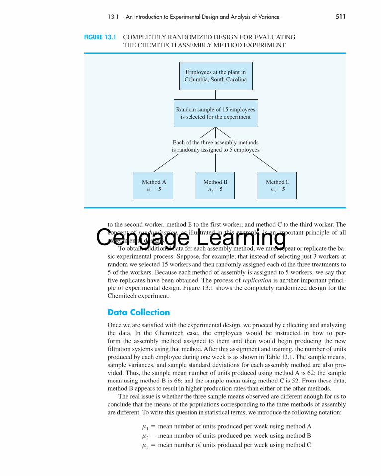
13.1 An Introduction to Experimental Design and Analysis of Variance 511
to the second worker, method B to the first worker, and method C to the third worker. Theconcept of randomization, as illustrated in this example, is an important principle of allexperimental designs.
To obtain additional data for each assembly method, we must repeat or replicate the ba-sic experimental process. Suppose, for example, that instead of selecting just 3 workers atrandom we selected 15 workers and then randomly assigned each of the three treatments to5 of the workers. Because each method of assembly is assigned to 5 workers, we say thatfive replicates have been obtained. The process of replication is another important princi-ple of experimental design. Figure 13.1 shows the completely randomized design for theChemitech experiment.
Data CollectionOnce we are satisfied with the experimental design, we proceed by collecting and analyzingthe data. In the Chemitech case, the employees would be instructed in how to per-form the assembly method assigned to them and then would begin producing the newfiltration systems using that method. After this assignment and training, the number of unitsproduced by each employee during one week is as shown in Table 13.1. The sample means,sample variances, and sample standard deviations for each assembly method are also pro-vided. Thus, the sample mean number of units produced using method A is 62; the samplemean using method B is 66; and the sample mean using method C is 52. From these data,method B appears to result in higher production rates than either of the other methods.
The real issue is whether the three sample means observed are different enough for us toconclude that the means of the populations corresponding to the three methods of assemblyare different. To write this question in statistical terms, we introduce the following notation:
µ1 � mean number of units produced per week using method A
µ2 � mean number of units produced per week using method B
µ3 � mean number of units produced per week using method C
Employees at the plant inColumbia, South Carolina
Random sample of 15 employeesis selected for the experiment
Method Bn2 = 5
Method An1 = 5
Method Cn3 = 5
Each of the three assembly methodsis randomly assigned to 5 employees
FIGURE 13.1 COMPLETELY RANDOMIZED DESIGN FOR EVALUATING THE CHEMITECH ASSEMBLY METHOD EXPERIMENT
56130_13_ch13_p508-560.qxd 2/22/08 11:04 PM Page 511
Cengage Learning
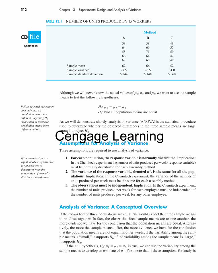
512 Chapter 13 Experimental Design and Analysis of Variance
Although we will never know the actual values of µ1, µ2, and µ3, we want to use the samplemeans to test the following hypotheses.
As we will demonstrate shortly, analysis of variance (ANOVA) is the statistical procedureused to determine whether the observed differences in the three sample means are largeenough to reject H0.
Assumptions for Analysis of VarianceThree assumptions are required to use analysis of variance.
1. For each population, the response variable is normally distributed. Implication:In the Chemitech experiment the number of units produced per week (response variable)must be normally distributed for each assembly method.
2. The variance of the response variable, denoted σ 2, is the same for all the pop-ulations. Implication: In the Chemitech experiment, the variance of the number ofunits produced per week must be the same for each assembly method.
3. The observations must be independent. Implication: In the Chemitech experiment,the number of units produced per week for each employee must be independent ofthe number of units produced per week for any other employee.
Analysis of Variance: A Conceptual OverviewIf the means for the three populations are equal, we would expect the three sample meansto be close together. In fact, the closer the three sample means are to one another, themore evidence we have for the conclusion that the population means are equal. Alterna-tively, the more the sample means differ, the more evidence we have for the conclusionthat the population means are not equal. In other words, if the variability among the sam-ple means is “small,” it supports H0; if the variability among the sample means is “large,”it supports Ha.
If the null hypothesis, H0: µ1 � µ2 � µ3, is true, we can use the variability among thesample means to develop an estimate of σ 2. First, note that if the assumptions for analysis
H0:
Ha: µ1 � µ2 � µ3
Not all population means are equal
If H0 is rejected, we cannotconclude that allpopulation means aredifferent. Rejecting H0
means that at least twopopulation means havedifferent values.
If the sample sizes areequal, analysis of varianceis not sensitive todepartures from theassumption of normallydistributed populations.
Method
A B C58 58 4864 69 5755 71 5966 64 4767 68 49
Sample mean 62 66 52Sample variance 27.5 26.5 31.0Sample standard deviation 5.244 5.148 5.568
TABLE 13.1 NUMBER OF UNITS PRODUCED BY 15 WORKERS
fileCDChemitech
56130_13_ch13_p508-560.qxd 2/22/08 11:04 PM Page 512
Cengage Learning
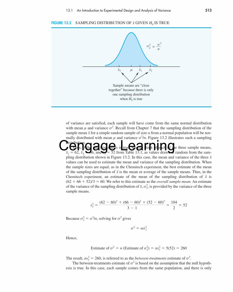
13.1 An Introduction to Experimental Design and Analysis of Variance 513
of variance are satisfied, each sample will have come from the same normal distributionwith mean µ and variance σ 2. Recall from Chapter 7 that the sampling distribution of thesample mean for a simple random sample of size n from a normal population will be nor-mally distributed with mean µ and variance σ 2/n. Figure 13.2 illustrates such a samplingdistribution.
Thus, if the null hypothesis is true, we can think of each of the three sample means,
1 � 62, 2 � 66, and 3 � 52 from Table 13.1, as values drawn at random from the sam-pling distribution shown in Figure 13.2. In this case, the mean and variance of the three values can be used to estimate the mean and variance of the sampling distribution. Whenthe sample sizes are equal, as in the Chemitech experiment, the best estimate of the meanof the sampling distribution of is the mean or average of the sample means. Thus, in theChemitech experiment, an estimate of the mean of the sampling distribution of is(62 � 66 � 52)/3 � 60. We refer to this estimate as the overall sample mean. An estimateof the variance of the sampling distribution of , , is provided by the variance of the threesample means.
Because � σ 2/n, solving for σ 2 gives
Hence,
The result, � 260, is referred to as the between-treatments estimate of σ 2.The between-treatments estimate of σ2 is based on the assumption that the null hypoth-
esis is true. In this case, each sample comes from the same population, and there is only
ns2x̄
Estimate of σ 2 � n (Estimate of σ 2x̄) � ns2
x̄ � 5(52) � 260
σ 2 � nσ 2x̄
σ 2x̄
s2x̄ �
(62 � 60)2 � (66 � 60)2 � (52 � 60)2
3 � 1�
104
2� 52
σ 2x̄x̄
x̄x̄
x̄x̄x̄x̄
x̄
2
x1
Sample means are “closetogether” because there is only
one sampling distributionwhen H0 is true
µ x2x3
=n
σ x
2σ
FIGURE 13.2 SAMPLING DISTRIBUTION OF GIVEN H0 IS TRUEx̄
56130_13_ch13_p508-560.qxd 2/22/08 11:04 PM Page 513
Cengage Learning
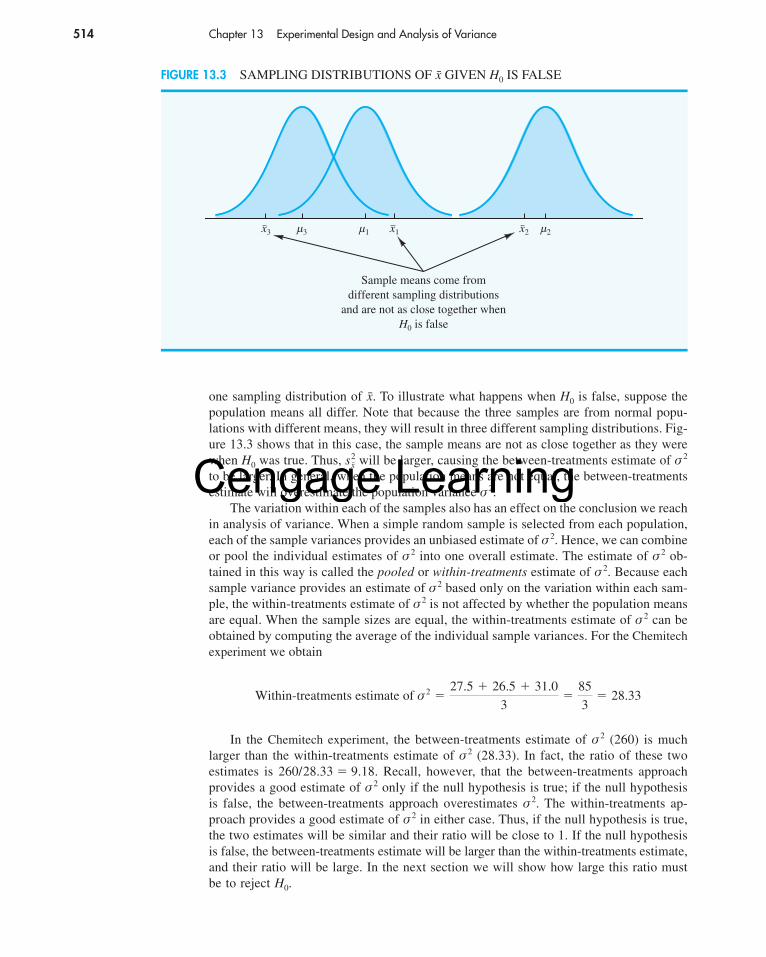
514 Chapter 13 Experimental Design and Analysis of Variance
one sampling distribution of . To illustrate what happens when H0 is false, suppose thepopulation means all differ. Note that because the three samples are from normal popu-lations with different means, they will result in three different sampling distributions. Fig-ure 13.3 shows that in this case, the sample means are not as close together as they werewhen H0 was true. Thus, will be larger, causing the between-treatments estimate of σ 2
to be larger. In general, when the population means are not equal, the between-treatmentsestimate will overestimate the population variance σ 2.
The variation within each of the samples also has an effect on the conclusion we reachin analysis of variance. When a simple random sample is selected from each population,each of the sample variances provides an unbiased estimate of σ 2. Hence, we can combineor pool the individual estimates of σ 2 into one overall estimate. The estimate of σ 2 ob-tained in this way is called the pooled or within-treatments estimate of σ 2. Because eachsample variance provides an estimate of σ 2 based only on the variation within each sam-ple, the within-treatments estimate of σ 2 is not affected by whether the population meansare equal. When the sample sizes are equal, the within-treatments estimate of σ 2 can beobtained by computing the average of the individual sample variances. For the Chemitechexperiment we obtain
In the Chemitech experiment, the between-treatments estimate of σ 2 (260) is muchlarger than the within-treatments estimate of σ 2 (28.33). In fact, the ratio of these twoestimates is 260/28.33 � 9.18. Recall, however, that the between-treatments approachprovides a good estimate of σ 2 only if the null hypothesis is true; if the null hypothesisis false, the between-treatments approach overestimates σ 2. The within-treatments ap-proach provides a good estimate of σ 2 in either case. Thus, if the null hypothesis is true,the two estimates will be similar and their ratio will be close to 1. If the null hypothesisis false, the between-treatments estimate will be larger than the within-treatments estimate,and their ratio will be large. In the next section we will show how large this ratio mustbe to reject H0.
Within-treatments estimate of σ 2 �27.5 � 26.5 � 31.0
3�
85
3� 28.33
s2x̄
x̄
µ1 x2x1x3 µ3 µ2
Sample means come fromdifferent sampling distributions
and are not as close together whenH0 is false
FIGURE 13.3 SAMPLING DISTRIBUTIONS OF GIVEN H0 IS FALSEx̄
56130_13_ch13_p508-560.qxd 2/22/08 11:04 PM Page 514
Cengage Learning
13.2 Analysis of Variance and the Completely Randomized Design 515
NOTES AND COMMENTS
1. Randomization in experimental design is theanalog of probability sampling in an observa-tional study.
2. In many medical experiments, potential biasis eliminated by using a double-blind experi-mental design. With this design, neither thephysician applying the treatment nor the sub-ject knows which treatment is being applied.Many other types of experiments could bene-fit from this type of design.
3. In this section we provided a conceptualoverview of how analysis of variance can beused to test for the equality of k population
means for a completely randomized experi-mental design. We will see that the same pro-cedure can also be used to test for the equalityof k population means for an observational ornonexperimental study.
4. In Sections 10.1 and 10.2 we presented statis-tical methods for testing the hypothesis that themeans of two populations are equal. ANOVAcan also be used to test the hypothesis that themeans of two populations are equal. In prac-tice, however, analysis of variance is usuallynot used except when dealing with three ormore population means.
13.2 Analysis of Variance and the CompletelyRandomized DesignIn this section we show how analysis of variance can be used to test for the equality of kpopulation means for a completely randomized design. The general form of the hypothesestested is
where
We assume that a simple random sample of size nj has been selected from each of the k popu-lations or treatments. For the resulting sample data, let
x ij �
nj �
x̄j �
s2j �
sj �
value of observation i for treatment j
number of observations for treatment j
sample mean for treatment j
sample variance for treatment j
sample standard deviation for treatment j
µj � mean of the jth population
H0:
Ha: µ1 � µ2 � . . . � µk
Not all population means are equal
In summary, the logic behind ANOVA is based on the development of two independentestimates of the common population variance σ 2. One estimate of σ 2 is based on the vari-ability among the sample means themselves, and the other estimate of σ 2 is based on thevariability of the data within each sample. By comparing these two estimates of σ 2, we willbe able to determine whether the population means are equal.
56130_13_ch13_p508-560.qxd 2/22/08 11:04 PM Page 515
Cengage Learning
516 Chapter 13 Experimental Design and Analysis of Variance
The formulas for the sample mean and sample variance for treatment j are as follows:
(13.1)
(13.2)
The overall sample mean, denoted , is the sum of all the observations divided by the totalnumber of observations. That is,
(13.3)
where
(13.4)
If the size of each sample is n, nT � kn; in this case equation (13.3) reduces to
(13.5)
In other words, whenever the sample sizes are the same, the overall sample mean is just theaverage of the k sample means.
Because each sample in the Chemitech experiment consists of n � 5 observations, theoverall sample mean can be computed by using equation (13.5). For the data in Table 13.1we obtained the following result:
If the null hypothesis is true ( µ1 � µ2 � µ3 � µ), the overall sample mean of 60 is the bestestimate of the population mean µ.
Between-Treatments Estimate of Population VarianceIn the preceding section, we introduced the concept of a between-treatments estimate of σ 2
and showed how to compute it when the sample sizes were equal. This estimate of σ 2 iscalled the mean square due to treatments and is denoted MSTR. The general formula forcomputing MSTR is
(13.6)
The numerator in equation (13.6) is called the sum of squares due to treatments and isdenoted SSTR. The denominator, k � 1, represents the degrees of freedom associatedwith SSTR. Hence, the mean square due to treatments can be computed using the followingformula.
MSTR �
�k
j�1
nj (x̄
j � x̄̄ )2
k � 1
x̄̄ �62 � 66 � 52
3� 60
x̄̄ �
�k
j�1
�nj
i�1
x ij
kn�
�k
j�1
�nj
i�1
x ij�n
k�
�k
j�1
x̄ j
k
nT � n1 � n2 � . . . � nk
x̄̄ �
�k
j�1
�nj
i�1
x ij
nT
x̄̄
s2j �
�nj
i�1
(x ij � x̄
j)2
nj � 1
x̄j ��
nj
i�1 x
ij
nj
56130_13_ch13_p508-560.qxd 2/22/08 11:04 PM Page 516
Cengage Learning

13.2 Analysis of Variance and the Completely Randomized Design 517
MEAN SQUARE DUE TO TREATMENTS
(13.7)
where
(13.8)SSTR � �k
j�1
nj (x̄
j � x̄̄ )2
MSTR �SSTR
k � 1
MEAN SQUARE DUE TO ERROR
(13.10)
where
(13.11)SSE � �k
j�1
(nj � 1)s2j
MSE �SSE
nT � k
If H0 is true, MSTR provides an unbiased estimate of σ 2. However, if the means of the kpopulations are not equal, MSTR is not an unbiased estimate of σ 2; in fact, in that case,MSTR should overestimate σ 2.
For the Chemitech data in Table 13.1, we obtain the following results:
Within-Treatments Estimate of Population VarianceEarlier, we introduced the concept of a within-treatments estimate of σ 2 and showed howto compute it when the sample sizes were equal. This estimate of σ 2 is called the meansquare due to error and is denoted MSE. The general formula for computing MSE is
(13.9)
The numerator in equation (13.9) is called the sum of squares due to error and is denotedSSE. The denominator of MSE is referred to as the degrees of freedom associated with SSE.Hence, the formula for MSE can also be stated as follows.
MSE �
�k
j�1
(nj � 1)s2j
nT � k
MSTR �SSTR
k � 1�
520
2� 260
SSTR � �k
j�1
nj (x̄
j � x̄̄ )2 � 5(62 � 60)2 � 5(66 � 60)2 � 5(52 � 60)2 � 520
Note that MSE is based on the variation within each of the treatments; it is not influenced bywhether the null hypothesis is true. Thus, MSE always provides an unbiased estimate of σ 2.
For the Chemitech data in Table 13.1 we obtain the following results:
MSE �SSE
nT � k�
340
15 � 3�
340
12� 28.33
SSE � �k
j�1
(nj � 1)s2j � (5 � 1)27.5 � (5 � 1)26.5 � (5 � 1)31 � 340
56130_13_ch13_p508-560.qxd 2/22/08 11:04 PM Page 517
Cengage Learning
518 Chapter 13 Experimental Design and Analysis of Variance
Using Excel, p-value � FDIST(9.18,2,12) � .004.
Comparing the Variance Estimates: The F TestIf the null hypothesis is true, MSTR and MSE provide two independent, unbiased estimatesof σ 2. Based on the material covered in Chapter 11 we know that for normal populations,the sampling distribution of the ratio of two independent estimates of σ 2 follows an F dis-tribution. Hence, if the null hypothesis is true and the ANOVA assumptions are valid, thesampling distribution of MSTR/MSE is an F distribution with numerator degrees of free-dom equal to k � 1 and denominator degrees of freedom equal to nT � k. In other words,if the null hypothesis is true, the value of MSTR/MSE should appear to have been selectedfrom this F distribution.
However, if the null hypothesis is false, the value of MSTR/MSE will be inflated be-cause MSTR overestimates σ 2. Hence, we will reject H0 if the resulting value of MSTR/MSEappears to be too large to have been selected from an F distribution with k � 1 numeratordegrees of freedom and nT � k denominator degrees of freedom. Because the decision toreject H0 is based on the value of MSTR/MSE, the test statistic used to test for the equalityof k population means is as follows.
TEST STATISTIC FOR THE EQUALITY OF k POPULATION MEANS
(13.12)
The test statistic follows an F distribution with k � 1 degrees of freedom in thenumerator and nT � k degrees of freedom in the denominator.
F �MSTR
MSE
Let us return to the Chemitech experiment and use a level of significance α � .05 toconduct the hypothesis test. The value of the test statistic is
The numerator degrees of freedom is k � 1 � 3 � 1 � 2 and the denominator degrees offreedom is nT � k � 15 � 3 � 12. Because we will only reject the null hypothesis for largevalues of the test statistic, the p-value is the upper tail area of the F distribution to the rightof the test statistic F � 9.18. Figure 13.4 shows the sampling distribution of F � MSTR/MSE, the value of the test statistic, and the upper tail area that is the p-value for thehypothesis test.
From Table 4 of Appendix B we find the following areas in the upper tail of an F dis-tribution with 2 numerator degrees of freedom and 12 denominator degrees of freedom.
F �MSTR
MSE�
260
28.33� 9.18
Area in Upper Tail .10 .05 .025 .01
F Value (df1 � 2, df2 � 12) 2.81 3.89 5.10 6.93
F � 9.18
An introduction to the F distribution and the use of the F distributiontable were presented inSection 11.2.
Because F � 9.18 is greater than 6.93, the area in the upper tail at F � 9.18 is less than .01.Thus, the p-value is less than .01. Excel can be used to show that the exact p-value is .004.With p-value � α � .05, H0 is rejected. The test provides sufficient evidence to concludethat the means of the three populations are not equal. In other words, analysis of variancesupports the conclusion that the population mean number of units produced per week forthe three assembly methods are not equal.
56130_13_ch13_p508-560.qxd 2/22/08 11:04 PM Page 518
Cengage Learning
13.2 Analysis of Variance and the Completely Randomized Design 519
As with other hypothesis testing procedures, the critical value approach may also beused. With α � .05, the critical F value occurs with an area of .05 in the upper tail of an Fdistribution with 2 and 12 degrees of freedom. From the F distribution table, we findF.05 � 3.89. Hence, the appropriate upper tail rejection rule for the Chemitech experiment is
With F � 9.18, we reject H0 and conclude that the means of the three populations are notequal. A summary of the overall procedure for testing for the equality of k population meansfollows.
Reject H0 if F � 3.89
F = 9.18MSTR/MSE
p-value
Sampling distributionof MSTR/MSE
FIGURE 13.4 COMPUTATION OF p-VALUE USING THE SAMPLING DISTRIBUTION OF MSTR/MSE
TEST FOR THE EQUALITY OF k POPULATION MEANS
TEST STATISTIC
REJECTION RULE
where the value of Fα is based on an F distribution with k � 1 numerator degrees offreedom and nT � k denominator degrees of freedom.
p-value approach:
Critical value approach:
Reject H0 if p-value � αReject H0 if F � Fα
F �MSTR
MSE
H0:
Ha: µ1 � µ2 � . . . � µk
Not all population means are equal
ANOVA TableThe results of the preceding calculations can be displayed conveniently in a table referredto as the analysis of variance or ANOVA table. The general form of the ANOVA table fora completely randomized design is shown in Table 13.2; Table 13.3 is the correspondingANOVA table for the Chemitech experiment. The sum of squares associated with the sourceof variation referred to as “Total” is called the total sum of squares (SST). Note that the re-sults for the Chemitech experiment suggest that SST � SSTR � SSE, and that the degrees
56130_13_ch13_p508-560.qxd 2/22/08 11:04 PM Page 519
Cengage Learning

520 Chapter 13 Experimental Design and Analysis of Variance
of freedom associated with this total sum of squares is the sum of the degrees of freedomassociated with the sum of squares due to treatments and the sum of squares due to error.
We point out that SST divided by its degrees of freedom nT � 1 is nothing more thanthe overall sample variance that would be obtained if we treated the entire set of 15 obser-vations as one data set. With the entire data set as one sample, the formula for computingthe total sum of squares, SST, is
(13.13)
It can be shown that the results we observed for the analysis of variance table for theChemitech experiment also apply to other problems. That is,
(13.14)
In other words, SST can be partitioned into two sums of squares: the sum of squares due totreatments and the sum of squares due to error. Note also that the degrees of freedom cor-responding to SST, nT � 1, can be partitioned into the degrees of freedom corresponding toSSTR, k � 1, and the degrees of freedom corresponding to SSE, nT � k. The analysis ofvariance can be viewed as the process of partitioning the total sum of squares and the de-grees of freedom into their corresponding sources: treatments and error. Dividing the sumof squares by the appropriate degrees of freedom provides the variance estimates, theF value, and the p-value used to test the hypothesis of equal population means.
Using ExcelExcel’s Anova: Single Factor tool can be used to conduct a hypothesis test about the dif-ference between the population means for the Chemitech experiment. Refer to the Excelworksheet shown in Figure 13.5 as we describe the tasks involved.
Enter Data: Columns A, B, and C contain labels and the number of filtration systemsproduced per week for each method of assembly.
SST � SSTR � SSE
SST � �k
j�1
�nj
i�1
(x ij � x̄̄
)2
Source Sum Degrees Meanof Variation of Squares of Freedom Square F p-value
Treatments SSTR
Error SSE
Total SST nT � 1
MSE �SSE
nT � knT � k
MSTR
MSEMSTR �
SSTR
k � 1k � 1
TABLE 13.2 ANOVA TABLE FOR A COMPLETELY RANDOMIZED DESIGN
Source Sum Degrees Meanof Variation of Squares of Freedom Square F p-valueTreatments 520 2 260.00 9.18 .004Error 340 12 28.33
Total 860 14
TABLE 13.3 ANOVA TABLE FOR THE CHEMITECH EXPERIMENT
Analysis of variance can bethought of as a statisticalprocedure for partitioningthe total sum of squaresinto separate components.
56130_13_ch13_p508-560.qxd 2/22/08 11:04 PM Page 520
Cengage Learning

13.2 Analysis of Variance and the Completely Randomized Design 521
Apply Tools: The following steps describe how to use Excel’s Anova: Single Factor toolto test the hypothesis that the mean number of units produced per week is the same for allthree methods of assembly.
Step 1. Click the Data tab on the RibbonStep 2. In the Analysis group, click Data AnalysisStep 3. Choose Anova: Single Factor from the list of Analysis ToolsStep 4. When the Anova: Single Factor dialog box appears (see Figure 13.6),
Enter A1:C6 in the Input Range boxSelect Grouped By: ColumnsSelect Labels in First RowEnter .05 in the Alpha boxSelect Output RangeEnter A8 in the Output Range box (to identify the upper left corner of
the section of the worksheet where the output will appear)Click OK
The output, titled Anova: Single Factor, appears in cells A8:G22 of the worksheet. CellsA10:E14 provide a summary of the data. Note that the sample mean and sample variancefor each method of assembly are the same as shown in Table 13.1. The ANOVA table, shownin cells A17:G22, is basically the same as the ANOVA table shown in Table 13.2. Excelidentifies the treatments source of variation using the label Between Groups and the errorsource of variation using the label Within Groups. In addition, the Excel output provides thep-value associated with the test as well as the critical F value.
FIGURE 13.5 EXCEL’S ANOVA: SINGLE FACTOR TOOL OUTPUT FOR THE CHEMITECHEXPERIMENT
A B C D E F G H1 Method A Method B Method C2 58 58 483 64 69 574 55 71 595 66 64 476 67 68 4978 Anova: Single Factor910 SUMMARY11 Groups Count Sum Average Variance12 Method A 5 310 62 27.513 Method B 5 330 66 26.514 Method C 5 260 52 31151617 ANOVA18 Source of Variation SS df MS F P-value F crit19 Between Groups 520 2 260 9.1765 0.0038 3.885320 Within Groups 340 12 28.33332122 Total 860 142324
56130_13_ch13_p508-560.qxd 2/22/08 11:04 PM Page 521
Cengage Learning

522 Chapter 13 Experimental Design and Analysis of Variance
We can use the p-value shown in cell F19, 0.0038, to make the hypothesis testing de-cision. Thus, at the α � .05 level of significance, we reject H0 because the p-value �0.0038 � α � .05. Hence, using the p-value approach we still conclude that the mean num-ber of units produced per week are not the same for the three assembly methods.
Testing for the Equality of k Population Means: An Observational StudyWe have shown how analysis of variance can be used to test for the equality of k populationmeans for a completely randomized experimental design. It is important to understand thatANOVA can also be used to test for the equality of three or more population means usingdata obtained from an observational study. As an example, let us consider the situation atNational Computer Products, Inc. (NCP).
NCP manufactures printers and fax machines at plants located in Atlanta, Dallas, andSeattle. To measure how much employees at these plants know about quality management,a random sample of 6 employees was selected from each plant and the employees selectedwere given a quality awareness examination. The examination scores for these 18 employ-ees are shown in Table 13.4. The sample means, sample variances, and sample standarddeviations for each group are also provided. Managers want to use these data to test thehypothesis that the mean examination score is the same for all three plants.
We define population 1 as all employees at the Atlanta plant, population 2 as allemployees at the Dallas plant, and population 3 as all employees at the Seattle plant. Let
�1 � mean examination score for population 1
�2 � mean examination score for population 2
�3 � mean examination score for population 3
Although we will never know the actual values of �1, �2, and �3, we want to use the sampleresults to test the following hypotheses:
H0: �1 � �2 � �3
Ha: Not all population means are equal
FIGURE 13.6 DIALOG BOX FOR ANOVA: SINGLE FACTOR
56130_13_ch13_p508-560.qxd 2/22/08 11:04 PM Page 522
Cengage Learning

13.2 Analysis of Variance and the Completely Randomized Design 523
Note that the hypothesis test for the NCP observational study is exactly the same as thehypothesis test for the Chemitech experiment. Indeed, the same analysis of variancemethodology we used to analyze the Chemitech experiment can also be used to analyze thedata from the NCP observational study.
Even though the sameANOVAmethodology is used for the analysis, it is worth noting howthe NCP observational statistical study differs from the Chemitech experimental statisticalstudy. The individuals who conducted the NCP study had no control over how the plants wereassigned to individual employees. That is, the plants were already in operation and a particularemployee worked at one of the three plants.All that NCPcould do was to select a random sam-ple of 6 employees from each plant and administer the quality awareness examination. To beclassified as an experimental study, NCP would have had to be able to randomly select 18 em-ployees and then assign the plants to each employee in a random fashion.
Plant 1 Plant 2 Plant 3Atlanta Dallas Seattle
85 71 5975 75 6482 73 6276 74 6971 69 7585 82 67
Sample mean 79 74 66Sample variance 34 20 32Sample standard deviation 5.83 4.47 5.66
TABLE 13.4 EXAMINATION SCORES FOR 18 EMPLOYEES
Exercise 8 will ask you toanalyze the NCP data usingthe analysis of varianceprocedure.
fileCDNCP
NOTES AND COMMENTS
1. The overall sample mean can also be computedas a weighted average of the k sample means.
In problems where the sample means are pro-vided, this formula is simpler thanequation(13.3)for computing the overall mean.
2. If each sample consists of n observations, equa-tion (13.6) can be written as
Note that this result is the same as presented inSection 13.1 when we introduced the concept
� ns2x̄
MSTR �
n �k
j� 1
(x̄ j � x̄̄)2
k � 1� n��
k
j� 1
(x̄ j � x̄̄)2
k � 1�
x̄̄ �n1x̄1 � n2 x̄2 � . . . � nk
x̄k
nT
of the between-treatments estimate of σ 2. Equa-tion (13.6) is simply a generalization of this resultto the unequal sample-size case.
3. If each sample has n observations, nT � kn;thus, nT � k � k(n � 1), and equation (13.9) canbe rewritten as
In other words, if the sample sizes are thesame, MSE is just the average of the k samplevariances. Note that it is the same result weused in Section 13.1 when we introducedthe concept of the within-treatments estimateof σ2.
MSE �
�k
j� 1
(n � 1)s2j
k(n � 1)�
(n � 1) �k
j� 1
s2j
k(n � 1)�
�k
j� 1
s2j
k
56130_13_ch13_p508-560.qxd 2/22/08 11:04 PM Page 523
Cengage Learning
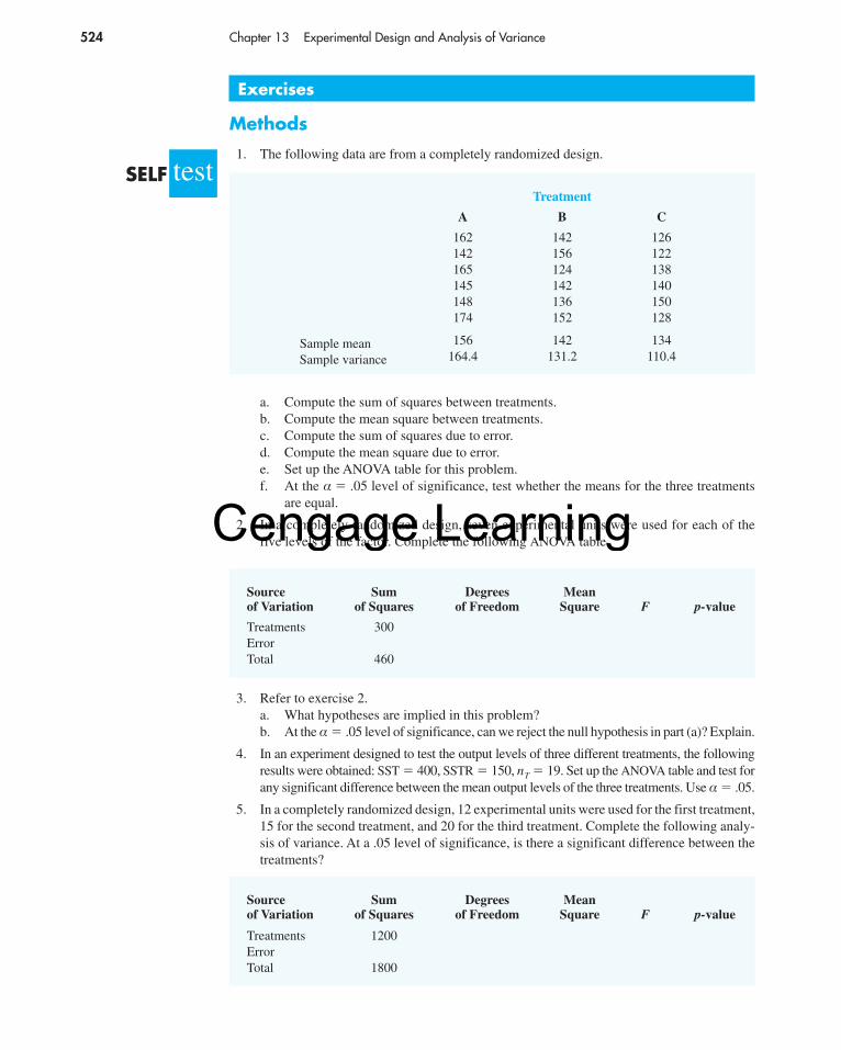
524 Chapter 13 Experimental Design and Analysis of Variance
Source Sum Degrees Meanof Variation of Squares of Freedom Square F p-value
Treatments 300 Error Total 460
Source Sum Degrees Meanof Variation of Squares of Freedom Square F p-value
Treatments 1200Error Total 1800
3. Refer to exercise 2.a. What hypotheses are implied in this problem?b. At the α � .05 level of significance, can we reject the null hypothesis in part (a)? Explain.
4. In an experiment designed to test the output levels of three different treatments, the followingresults were obtained: SST � 400, SSTR � 150, nT � 19. Set up the ANOVA table and test forany significant difference between the mean output levels of the three treatments. Use α � .05.
5. In a completely randomized design, 12 experimental units were used for the first treatment,15 for the second treatment, and 20 for the third treatment. Complete the following analy-sis of variance. At a .05 level of significance, is there a significant difference between thetreatments?
Treatment
A B C
162 142 126142 156 122165 124 138145 142 140148 136 150174 152 128
Sample mean 156 142 134
Sample variance 164.4 131.2 110.4
a. Compute the sum of squares between treatments.b. Compute the mean square between treatments.c. Compute the sum of squares due to error.d. Compute the mean square due to error.e. Set up the ANOVA table for this problem.f. At the α � .05 level of significance, test whether the means for the three treatments
are equal.
2. In a completely randomized design, seven experimental units were used for each of thefive levels of the factor. Complete the following ANOVA table.
Exercises
Methods1. The following data are from a completely randomized design.
testSELF
56130_13_ch13_p508-560.qxd 2/22/08 11:04 PM Page 524
Cengage Learning
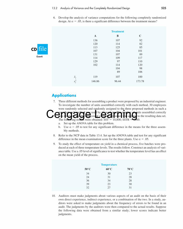
13.2 Analysis of Variance and the Completely Randomized Design 525
Applications7. Three different methods for assembling a product were proposed by an industrial engineer.
To investigate the number of units assembled correctly with each method, 30 employeeswere randomly selected and randomly assigned to the three proposed methods in such away that each method was used by 10 workers. The number of units assembled correctlywas recorded, and the analysis of variance procedure was applied to the resulting data set.The following results were obtained: SST � 10,800; SSTR � 4560.a. Set up the ANOVA table for this problem.b. Use α � .05 to test for any significant difference in the means for the three assem-
bly methods.
8. Refer to the NCP data in Table 13.4. Set up the ANOVA table and test for any significantdifference in the mean examination score for the three plants. Use α � .05.
9. To study the effect of temperature on yield in a chemical process, five batches were pro-duced at each of three temperature levels. The results follow. Construct an analysis of vari-ance table. Use a .05 level of significance to test whether the temperature level has an effecton the mean yield of the process.
Temperature
50°C 60°C 70°C
34 30 2324 31 2836 34 2839 23 3032 27 31
6. Develop the analysis of variance computations for the following completely randomizeddesign. At α � .05, is there a significant difference between the treatment means?
Treatment
A B C
136 107 92120 114 82113 125 85107 104 101131 107 89114 109 117129 97 110102 114 120
104 9889 106
119 107 100
146.86 96.44 173.78s2j
x̄j
fileCDExer6
10. Auditors must make judgments about various aspects of an audit on the basis of theirown direct experience, indirect experience, or a combination of the two. In a study, au-ditors were asked to make judgments about the frequency of errors to be found in anaudit. The judgments by the auditors were then compared to the actual results. Supposethe following data were obtained from a similar study; lower scores indicate betterjudgments.
56130_13_ch13_p508-560.qxd 2/22/08 11:04 PM Page 525
Cengage Learning
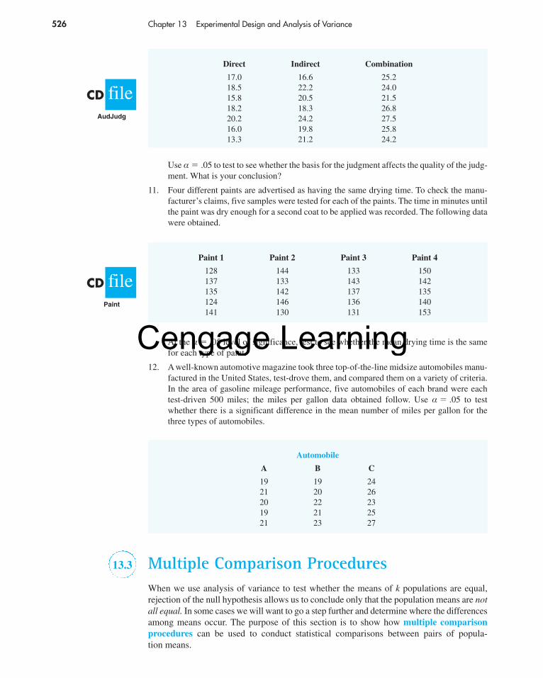
526 Chapter 13 Experimental Design and Analysis of Variance
At the α � .05 level of significance, test to see whether the mean drying time is the samefor each type of paint.
12. A well-known automotive magazine took three top-of-the-line midsize automobiles manu-factured in the United States, test-drove them, and compared them on a variety of criteria.In the area of gasoline mileage performance, five automobiles of each brand were eachtest-driven 500 miles; the miles per gallon data obtained follow. Use α � .05 to testwhether there is a significant difference in the mean number of miles per gallon for thethree types of automobiles.
Paint 1 Paint 2 Paint 3 Paint 4
128 144 133 150137 133 143 142135 142 137 135124 146 136 140141 130 131 153
fileCDPaint
Automobile
A B C
19 19 2421 20 2620 22 2319 21 2521 23 27
13.3 Multiple Comparison ProceduresWhen we use analysis of variance to test whether the means of k populations are equal,rejection of the null hypothesis allows us to conclude only that the population means are notall equal. In some cases we will want to go a step further and determine where the differencesamong means occur. The purpose of this section is to show how multiple comparisonprocedures can be used to conduct statistical comparisons between pairs of popula-tion means.
Use α � .05 to test to see whether the basis for the judgment affects the quality of the judg-ment. What is your conclusion?
11. Four different paints are advertised as having the same drying time. To check the manu-facturer’s claims, five samples were tested for each of the paints. The time in minutes untilthe paint was dry enough for a second coat to be applied was recorded. The following datawere obtained.
Direct Indirect Combination
17.0 16.6 25.218.5 22.2 24.015.8 20.5 21.518.2 18.3 26.820.2 24.2 27.516.0 19.8 25.813.3 21.2 24.2
fileCDAudJudg
56130_13_ch13_p508-560.qxd 2/22/08 11:04 PM Page 526
Cengage Learning

13.3 Multiple Comparison Procedures 527
Let us now apply this procedure to determine whether there is a significant differencebetween the means of population 1 (method A) and population 2 (method B) at the α � .05level of significance. Table 13.1 showed that the sample mean is 62 for method A and 66for method B. Table 13.3 showed that the value of MSE is 28.33; it is the estimate of σ2 andis based on 12 degrees of freedom. For the Chemitech data the value of the test statistic is
Because we have a two-tailed test, the p-value is two times the area under the curve forthe t distribution to the left of t � �1.19. Using Table 2 in Appendix B, the t distributiontable for 12 degrees of freedom provides the following information:
t �62 � 66
�28.33�1
5�
1
5�� �1.19
FISHER’S LSD PROCEDURE
TEST STATISTIC
(13.16)
REJECTION RULE
where the value of tα/2 is based on a t distribution with nT � k degrees of freedom.
p-value approach:
Critical value approach:
Reject H0 if p-value � αReject H0 if t � �tα/2 or t � tα/2
t �x̄i � x̄j
�MSE�1ni
�1nj�
H0:
Ha: µi � µj
µi � µj
Area in Upper Tail .20 .10 .05 .025 .01 .005
t Value (12 df ) .873 1.356 1.782 2.179 2.681 3.055
t � 1.19
Fisher’s LSDSuppose that analysis of variance provides statistical evidence to reject the null hypothesisof equal population means. In this case, Fisher’s least significant difference (LSD) proce-dure can be used to determine where the differences occur. To illustrate the use of Fisher’sLSD procedure in making pairwise comparisons of population means, recall the Chemitechexperiment introduced in Section 13.1. Using analysis of variance, we concluded that themean number of units produced per week are not the same for the three assembly methods.In this case, the follow-up question is: We believe the assembly methods differ, but wheredo the differences occur? That is, do the means of populations 1 and 2 differ? Or those ofpopulations 1 and 3? Or those of populations 2 and 3?
In Chapter 10 we presented a statistical procedure for testing the hypothesis that themeans of two populations are equal. With a slight modification in how we estimate thepopulation variance, Fisher’s LSD procedure is based on the t test statistic presented for the two-population case. The following table summarizes Fisher’s LSD procedure.
The t distribution table only contains positive t values. Because the t distribution is sym-metric, however, we can find the area under the curve to the right of t � 1.19 and doubleit to find the p-value corresponding to t � �1.19. We see that t � 1.19 is between .20 and
56130_13_ch13_p508-560.qxd 2/22/08 11:04 PM Page 527
Cengage Learning
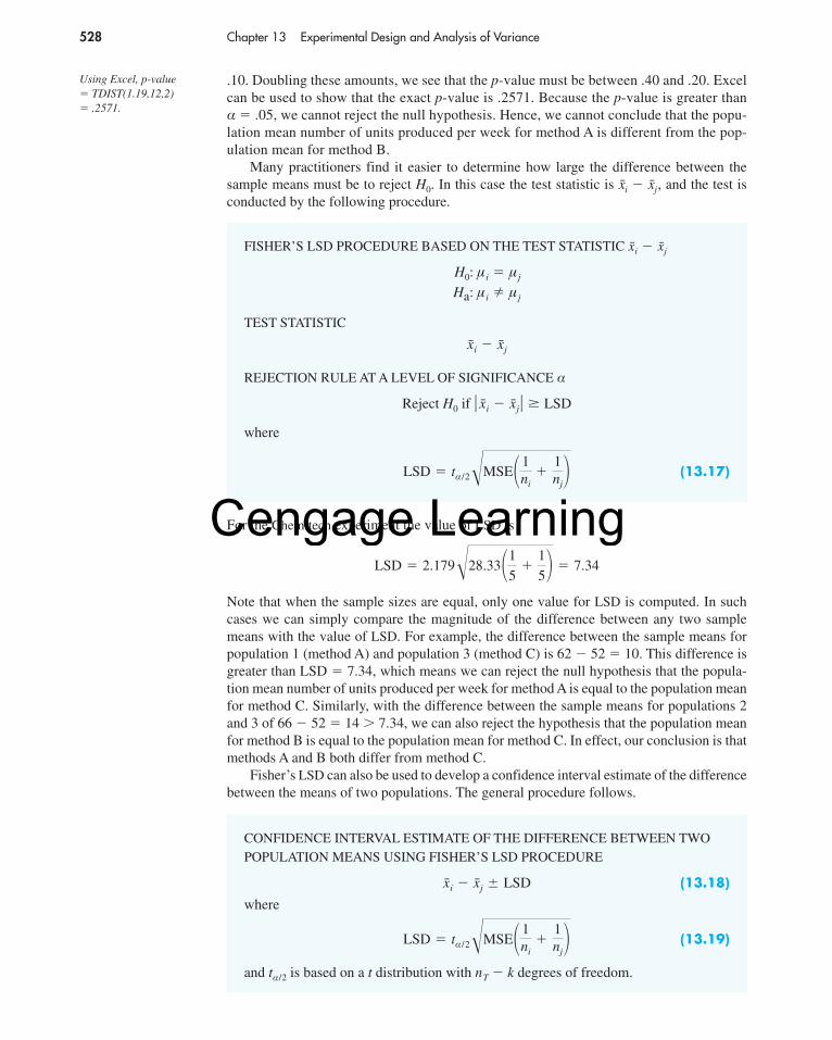
528 Chapter 13 Experimental Design and Analysis of Variance
For the Chemitech experiment the value of LSD is
Note that when the sample sizes are equal, only one value for LSD is computed. In suchcases we can simply compare the magnitude of the difference between any two samplemeans with the value of LSD. For example, the difference between the sample means forpopulation 1 (method A) and population 3 (method C) is 62 � 52 � 10. This difference isgreater than LSD � 7.34, which means we can reject the null hypothesis that the popula-tion mean number of units produced per week for method A is equal to the population meanfor method C. Similarly, with the difference between the sample means for populations 2and 3 of 66 � 52 � 14 � 7.34, we can also reject the hypothesis that the population meanfor method B is equal to the population mean for method C. In effect, our conclusion is thatmethods A and B both differ from method C.
Fisher’s LSD can also be used to develop a confidence interval estimate of the differencebetween the means of two populations. The general procedure follows.
LSD � 2.179�28.33�1
5�
1
5� � 7.34
FISHER’S LSD PROCEDURE BASED ON THE TEST STATISTIC
TEST STATISTIC
REJECTION RULE AT A LEVEL OF SIGNIFICANCE α
where
(13.17)LSD � tα/2�MSE�1ni
�1nj�
Reject H0 if � x̄i � x̄j� � LSD
x̄i � x̄j
H0:
Ha: µi � µj
µi � µj
x̄i � x̄j
CONFIDENCE INTERVAL ESTIMATE OF THE DIFFERENCE BETWEEN TWOPOPULATION MEANS USING FISHER’S LSD PROCEDURE
(13.18)
where
(13.19)
and tα/2 is based on a t distribution with nT � k degrees of freedom.
LSD � tα/2�MSE�1ni
�1nj�
x̄i � x̄j LSD
.10. Doubling these amounts, we see that the p-value must be between .40 and .20. Excelcan be used to show that the exact p-value is .2571. Because the p-value is greater thanα � .05, we cannot reject the null hypothesis. Hence, we cannot conclude that the popu-lation mean number of units produced per week for method A is different from the pop-ulation mean for method B.
Many practitioners find it easier to determine how large the difference between thesample means must be to reject H0. In this case the test statistic is and the test isconducted by the following procedure.
x̄i � x̄j,
Using Excel, p-value� TDIST(1.19,12,2) � .2571.
56130_13_ch13_p508-560.qxd 2/22/08 11:04 PM Page 528
Cengage Learning
13.3 Multiple Comparison Procedures 529
If the confidence interval in expression (13.18) includes the value zero, we cannot reject thehypothesis that the two population means are equal. However, if the confidence interval doesnot include the value zero, we conclude that there is a difference between the populationmeans. For the Chemitech experiment, recall that LSD � 7.34 (corresponding to t.025 � 2.179).Thus, a 95% confidence interval estimate of the difference between the means of populations1 and 2 is 62 � 66 7.34 � �4 7.34 � �11.34 to 3.34; because this interval includeszero, we cannot reject the hypothesis that the two population means are equal.
Type I Error RatesWe began the discussion of Fisher’s LSD procedure with the premise that analysis of vari-ance gave us statistical evidence to reject the null hypothesis of equal population means.We showed how Fisher’s LSD procedure can be used in such cases to determine wherethe differences occur. Technically, it is referred to as a protected or restricted LSD testbecause it is employed only if we first find a significant F value by using analysis of vari-ance. To see why this distinction is important in multiple comparison tests, we need toexplain the difference between a comparisonwise Type I error rate and an experimentwiseType I error rate.
In the Chemitech experiment we used Fisher’s LSD procedure to make three pairwisecomparisons:
Test 1 Test 2 Test 3
In each case, we used a level of significance of α � .05. Therefore, for each test, if the nullhypothesis is true, the probability that we will make a Type I error is α � .05; hence, theprobability that we will not make a Type I error on each test is 1 � .05 � .95. In discussingmultiple comparison procedures we refer to this probability of a Type I error (α � .05) asthe comparisonwise Type I error rate; comparisonwise Type I error rates indicate the level of significance associated with a single pairwise comparison.
Let us now consider a slightly different question. What is the probability that inmaking three pairwise comparisons, we will commit a Type I error on at least one of thethree tests? To answer this question, note that the probability that we will not make a TypeI error on any of the three tests is (.95)(.95)(.95) � .8574.1 Therefore, the probability ofmaking at least one Type I error is 1 � .8574 � .1426. Thus, when we use Fisher’s LSDprocedure to make all three pairwise comparisons, the Type I error rate associated withthis approach is not .05, but actually .1426; we refer to this error rate as the overall orexperimentwise Type I error rate. To avoid confusion, we denote the experimentwiseType I error rate as αEW.
The experimentwise Type I error rate gets larger for problems with more populations.For example, a problem with five populations has 10 possible pairwise comparisons. If wetested all possible pairwise comparisons by using Fisher’s LSD with a comparisonwise errorrate of α � .05, the experimentwise Type I error rate would be 1 � (1 � .05)10 � .40. Insuch cases, practitioners look to alternatives that provide better control over the experi-mentwise error rate.
One alternative for controlling the overall experimentwise error rate, referred to as theBonferroni adjustment, involves using a smaller comparisonwise error rate for each test. Forexample, if we want to test C pairwise comparisons and want the maximum probability ofmaking a Type I error for the overall experiment to be αEW, we simply use a comparisonwise
H0:
Ha: µ2 � µ3
µ2 � µ3
H0:
Ha: µ1 � µ3
µ1 � µ3
H0:
Ha: µ1 � µ2
µ1 � µ2
1The assumption is that the three tests are independent, and hence the joint probability of the three events can be obtainedby simply multiplying the individual probabilities. In fact, the three tests are not independent because MSE is used in each test;therefore, the error involved is even greater than that shown.
56130_13_ch13_p508-560.qxd 2/22/08 11:04 PM Page 529
Cengage Learning
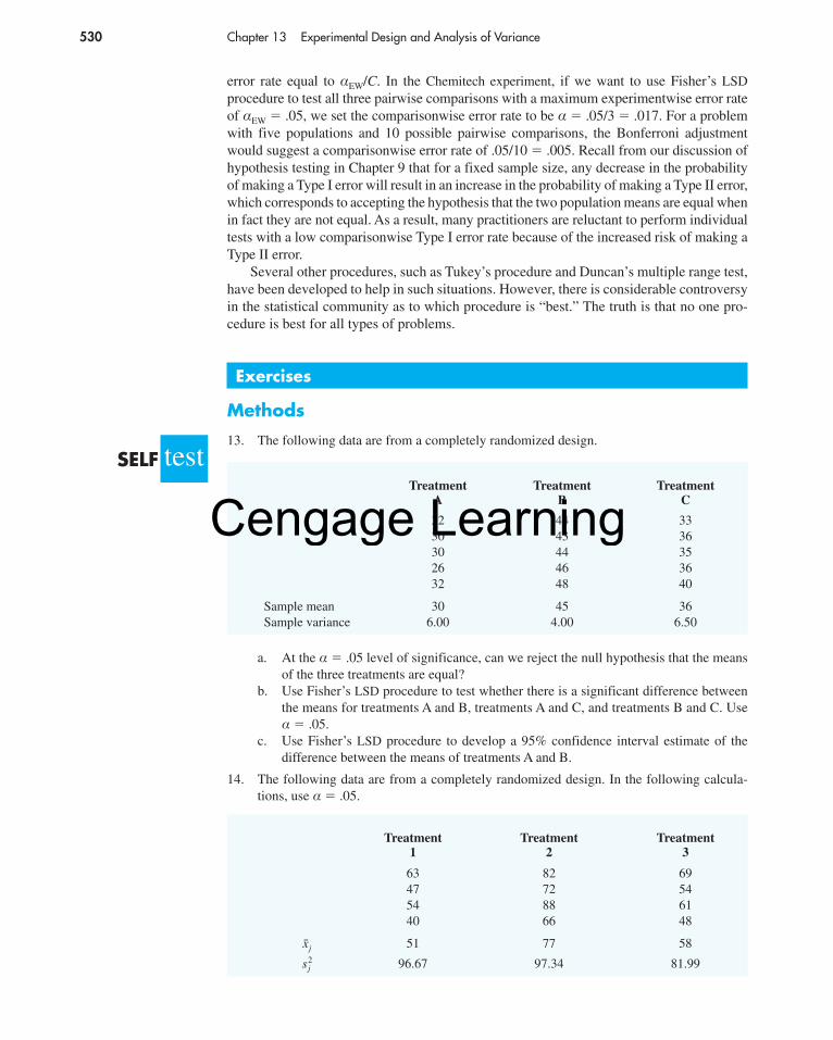
530 Chapter 13 Experimental Design and Analysis of Variance
error rate equal to αEW/C. In the Chemitech experiment, if we want to use Fisher’s LSDprocedure to test all three pairwise comparisons with a maximum experimentwise error rateof αEW � .05, we set the comparisonwise error rate to be α � .05/3 � .017. For a problemwith five populations and 10 possible pairwise comparisons, the Bonferroni adjustmentwould suggest a comparisonwise error rate of .05/10 � .005. Recall from our discussion ofhypothesis testing in Chapter 9 that for a fixed sample size, any decrease in the probabilityof making a Type I error will result in an increase in the probability of making a Type II error,which corresponds to accepting the hypothesis that the two population means are equal whenin fact they are not equal. As a result, many practitioners are reluctant to perform individualtests with a low comparisonwise Type I error rate because of the increased risk of making aType II error.
Several other procedures, such as Tukey’s procedure and Duncan’s multiple range test,have been developed to help in such situations. However, there is considerable controversyin the statistical community as to which procedure is “best.” The truth is that no one pro-cedure is best for all types of problems.
Exercises
Methods13. The following data are from a completely randomized design.
a. At the α � .05 level of significance, can we reject the null hypothesis that the meansof the three treatments are equal?
b. Use Fisher’s LSD procedure to test whether there is a significant difference betweenthe means for treatments A and B, treatments A and C, and treatments B and C. Useα � .05.
c. Use Fisher’s LSD procedure to develop a 95% confidence interval estimate of thedifference between the means of treatments A and B.
14. The following data are from a completely randomized design. In the following calcula-tions, use α � .05.
testSELFTreatment Treatment Treatment
A B C
32 44 3330 43 3630 44 3526 46 3632 48 40
Sample mean 30 45 36Sample variance 6.00 4.00 6.50
Treatment Treatment Treatment 1 2 3
63 82 6947 72 5454 88 6140 66 48
51 77 58
96.67 97.34 81.99s2j
x̄j
56130_13_ch13_p508-560.qxd 2/22/08 11:04 PM Page 530
Cengage Learning

13.3 Multiple Comparison Procedures 531
a. Use analysis of variance to test for a significant difference among the means of thethree treatments.
b. Use Fisher’s LSD procedure to determine which means are different.
Applications15. To test whether the mean time needed to mix a batch of material is the same for machines
produced by three manufacturers, the Jacobs Chemical Company obtained the following dataon the time (in minutes) needed to mix the material.
Manufacturer
1 2 3
20 28 2026 26 1924 31 2322 27 22
a. Use these data to test whether the population mean times for mixing a batch of materialdiffer for the three manufacturers. Use α � .05.
b. At the α � .05 level of significance, use Fisher’s LSD procedure to test for the equalityof the means for manufacturers 1 and 3. What conclusion can you draw after carryingout this test?
16. Refer to exercise 15. Use Fisher’s LSD procedure to develop a 95% confidence intervalestimate of the difference between the means for manufacturer 1 and manufacturer 2.
17. The following data are from an experiment designed to investigate the perception of cor-porate ethical values among individuals specializing in marketing (higher scores indicatehigher ethical values).
Marketing Managers Marketing Research Advertising
6 5 65 5 74 4 65 4 56 5 64 4 6
a. Use α � .05 to test for significant differences in perception among the three groups.b. At the α � .05 level of significance, we can conclude that there are differences in the
perceptions for marketing managers, marketing research specialists, and advertisingspecialists. Use the procedures in this section to determine where the differencesoccur. Use α � .05.
18. To test for any significant difference in the number of hours between breakdowns for fourmachines, the following data were obtained.
testSELF
testSELF
Machine 1 Machine 2 Machine 3 Machine 4
6.4 8.7 11.1 9.97.8 7.4 10.3 12.85.3 9.4 9.7 12.17.4 10.1 10.3 10.88.4 9.2 9.2 11.37.3 9.8 8.8 11.5
56130_13_ch13_p508-560.qxd 2/22/08 11:04 PM Page 531
Cengage Learning

532 Chapter 13 Experimental Design and Analysis of Variance
a. At the α � .05 level of significance, what is the difference, if any, in the populationmean times among the four machines?
b. Use Fisher’s LSD procedure to test for the equality of the means for machines 2 and4. Use a .05 level of significance.
19. Refer to exercise 18. Use the Bonferroni adjustment to test for a significant differencebetween all pairs of means. Assume that a maximum overall experimentwise error rate of.05 is desired.
20. Condé Nast Traveler conducts an annual survey in which readers rate their favorite cruiseships. Ratings are provided for small ships (carrying up to 500 passengers), medium ships(carrying more than 500 but less than 1500 passengers), and large ships (carrying a mini-mum of 1500 passengers). The following data show the service ratings for eight randomlyselected small ships, eight randomly selected medium ships, and eight randomly selectedlarge ships. All ships are rated on a 100-point scale, with higher values indicating betterservice (Condé Nast Traveler, February 2003).
a. Use α � .05 to test for any significant difference in the mean service ratings amongthe three sizes of cruise ships.
b. Use the procedures in this section to determine where the differences occur. Use α � .05.
13.4 Randomized Block DesignThus far we have considered the completely randomized experimental design. Recall thatto test for a difference among treatment means, we computed an F value by using the ratio
(13.20)
A problem can arise whenever differences due to extraneous factors (ones not consid-ered in the experiment) cause the MSE term in this ratio to become large. In such cases, theF value in equation (13.20) can become small, signaling no difference among treatmentmeans when in fact such a difference exists.
In this section we present an experimental design known as a randomized blockdesign. Its purpose is to control some of the extraneous sources of variation by removingsuch variation from the MSE term. This design tends to provide a better estimate of the trueerror variance and leads to a more powerful hypothesis test in terms of the ability to detect
F �MSTR
MSE
Small Ships Medium Ships Large Ships
Name Rating Name Rating Name Rating
Hanseactic 90.5 Amsterdam 91.1 Century 89.2Mississippi Queen 78.2 Crystal Symphony 98.9 Disney Wonder 90.2Philae 92.3 Maasdam 94.2 Enchantment of the Seas 85.9Royal Clipper 95.7 Noordam 84.3 Grand Princess 84.2Seabourn Pride 94.1 Royal Princess 84.8 Infinity 90.2Seabourn Spirit 100 Ryndam 89.2 Legend of the Seas 80.6Silver Cloud 91.8 Statendam 86.4 Paradise 75.8Silver Wind 95 Veendam 88.3 Sun Princess 82.3
fileCDShips
A completely randomizeddesign is useful when theexperimental units arehomogeneous. If theexperimental units areheterogeneous, blocking isoften used to formhomogeneous groups.
56130_13_ch13_p508-560.qxd 2/22/08 11:04 PM Page 532
Cengage Learning
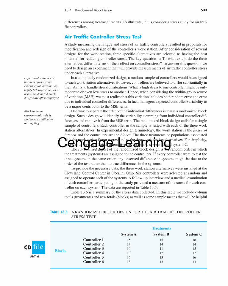
13.4 Randomized Block Design 533
differences among treatment means. To illustrate, let us consider a stress study for air traf-fic controllers.
Air Traffic Controller Stress TestA study measuring the fatigue and stress of air traffic controllers resulted in proposals formodification and redesign of the controller’s work station. After consideration of severaldesigns for the work station, three specific alternatives are selected as having the bestpotential for reducing controller stress. The key question is: To what extent do the threealternatives differ in terms of their effect on controller stress? To answer this question, weneed to design an experiment that will provide measurements of air traffic controller stressunder each alternative.
In a completely randomized design, a random sample of controllers would be assignedto each work station alternative. However, controllers are believed to differ substantially intheir ability to handle stressful situations. What is high stress to one controller might be onlymoderate or even low stress to another. Hence, when considering the within-group sourceof variation (MSE), we must realize that this variation includes both random error and errordue to individual controller differences. In fact, managers expected controller variability tobe a major contributor to the MSE term.
One way to separate the effect of the individual differences is to use a randomized blockdesign. Such a design will identify the variability stemming from individual controller dif-ferences and remove it from the MSE term. The randomized block design calls for a singlesample of controllers. Each controller in the sample is tested with each of the three workstation alternatives. In experimental design terminology, the work station is the factor ofinterest and the controllers are the blocks. The three treatments or populations associatedwith the work station factor correspond to the three work station alternatives. For simplicity,we refer to the work station alternatives as system A, system B, and system C.
The randomized aspect of the randomized block design is the random order in whichthe treatments (systems) are assigned to the controllers. If every controller were to test thethree systems in the same order, any observed difference in systems might be due to theorder of the test rather than to true differences in the systems.
To provide the necessary data, the three work station alternatives were installed at theCleveland Control Center in Oberlin, Ohio. Six controllers were selected at random andassigned to operate each of the systems. A follow-up interview and a medical examinationof each controller participating in the study provided a measure of the stress for each con-troller on each system. The data are reported in Table 13.5.
Table 13.6 is a summary of the stress data collected. In this table we include columntotals (treatments) and row totals (blocks) as well as some sample means that will be helpful
Experimental studies inbusiness often involveexperimental units that arehighly heterogeneous; as aresult, randomized blockdesigns are often employed.
Blocking in anexperimental study issimilar to stratification in sampling.
Treatments
System A System B System CController 1 15 15 18Controller 2 14 14 14
Blocks Controller 3 10 11 15Controller 4 13 12 17Controller 5 16 13 16Controller 6 13 13 13
TABLE 13.5 A RANDOMIZED BLOCK DESIGN FOR THE AIR TRAFFIC CONTROLLERSTRESS TEST
fileCDAirTraf
56130_13_ch13_p508-560.qxd 2/22/08 11:04 PM Page 533
Cengage Learning
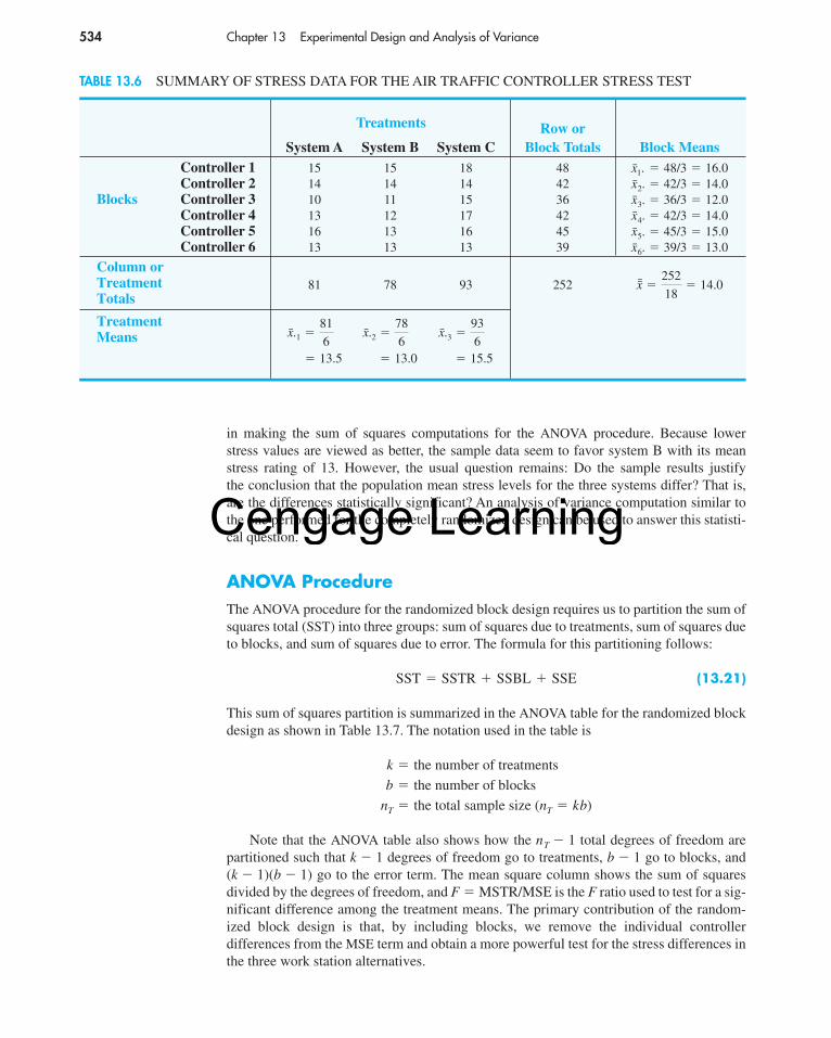
534 Chapter 13 Experimental Design and Analysis of Variance
in making the sum of squares computations for the ANOVA procedure. Because lowerstress values are viewed as better, the sample data seem to favor system B with its meanstress rating of 13. However, the usual question remains: Do the sample results justifythe conclusion that the population mean stress levels for the three systems differ? That is,are the differences statistically significant? An analysis of variance computation similar tothe one performed for the completely randomized design can be used to answer this statisti-cal question.
ANOVA ProcedureThe ANOVA procedure for the randomized block design requires us to partition the sum ofsquares total (SST) into three groups: sum of squares due to treatments, sum of squares dueto blocks, and sum of squares due to error. The formula for this partitioning follows:
(13.21)
This sum of squares partition is summarized in the ANOVA table for the randomized blockdesign as shown in Table 13.7. The notation used in the table is
Note that the ANOVA table also shows how the nT � 1 total degrees of freedom arepartitioned such that k � 1 degrees of freedom go to treatments, b � 1 go to blocks, and(k � 1)(b � 1) go to the error term. The mean square column shows the sum of squaresdivided by the degrees of freedom, and F � MSTR/MSE is the F ratio used to test for a sig-nificant difference among the treatment means. The primary contribution of the random-ized block design is that, by including blocks, we remove the individual controllerdifferences from the MSE term and obtain a more powerful test for the stress differences inthe three work station alternatives.
k �
b �
nT �
the number of treatments
the number of blocks
the total sample size (nT � kb)
SST � SSTR � SSBL � SSE
Treatments Row orSystem A System B System C Block Totals Block Means
Controller 1 15 15 18 48Controller 2 14 14 14 42
Blocks Controller 3 10 11 15 36Controller 4 13 12 17 42Controller 5 16 13 16 45Controller 6 13 13 13 39
81 78 93 252
� 15.5� 13.0� 13.5
x̄.3 �93
6x̄.2 �
78
6x̄.1 �
81
6
TreatmentMeans
x̄̄ �252
18� 14.0
Column orTreatmentTotals
x̄6. � 39/3 � 13.0x̄5. � 45/3 � 15.0x̄4. � 42/3 � 14.0x̄3. � 36/3 � 12.0x̄2. � 42/3 � 14.0x̄1. � 48/3 � 16.0
TABLE 13.6 SUMMARY OF STRESS DATA FOR THE AIR TRAFFIC CONTROLLER STRESS TEST
56130_13_ch13_p508-560.qxd 2/22/08 11:04 PM Page 534
Cengage Learning
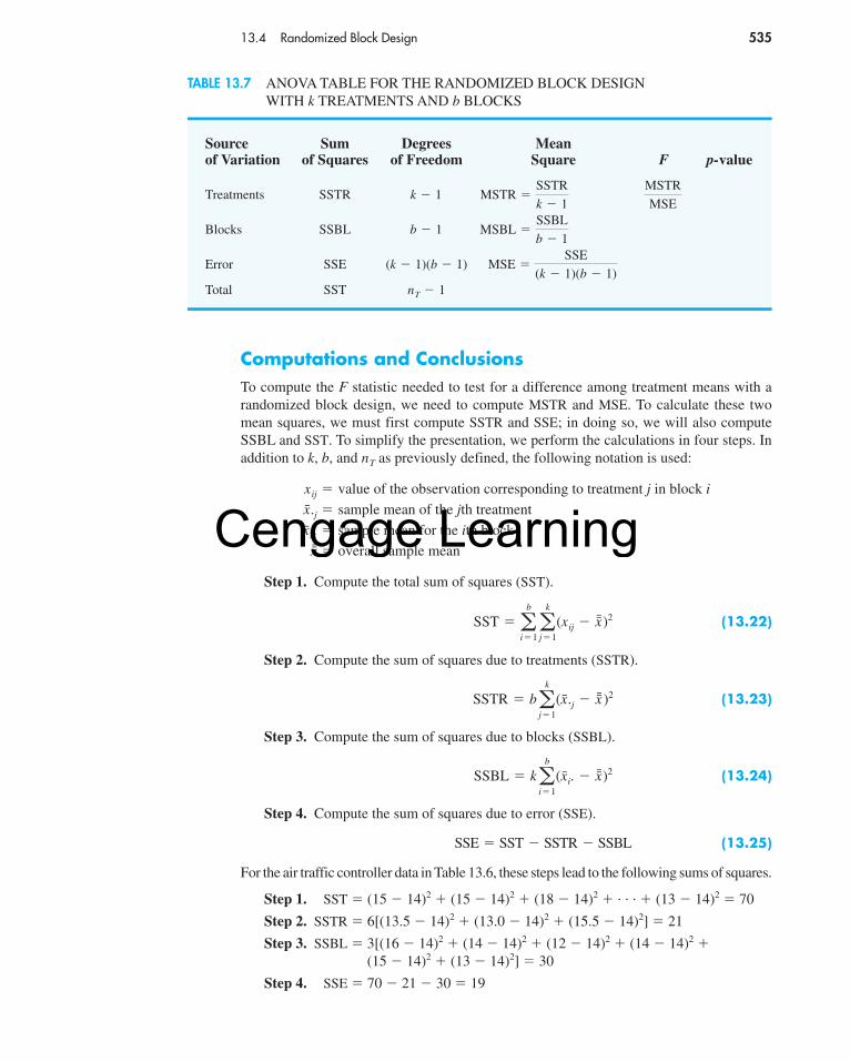
13.4 Randomized Block Design 535
Computations and ConclusionsTo compute the F statistic needed to test for a difference among treatment means with arandomized block design, we need to compute MSTR and MSE. To calculate these twomean squares, we must first compute SSTR and SSE; in doing so, we will also computeSSBL and SST. To simplify the presentation, we perform the calculations in four steps. Inaddition to k, b, and nT as previously defined, the following notation is used:
Step 1. Compute the total sum of squares (SST).
(13.22)
Step 2. Compute the sum of squares due to treatments (SSTR).
(13.23)
Step 3. Compute the sum of squares due to blocks (SSBL).
(13.24)
Step 4. Compute the sum of squares due to error (SSE).
(13.25)
For the air traffic controller data in Table 13.6, these steps lead to the following sums of squares.
Step 1. SST � (15 � 14)2 � (15 � 14)2 � (18 � 14)2 � . . . � (13 � 14)2 � 70
Step 2. SSTR � 6[(13.5 � 14)2 � (13.0 � 14)2 � (15.5 � 14)2] � 21
Step 3. SSBL � 3[(16 � 14)2 � (14 � 14)2 � (12 � 14)2 � (14 � 14)2 �(15 � 14)2 � (13 � 14)2] � 30
Step 4. SSE � 70 � 21 � 30 � 19
SSE � SST � SSTR � SSBL
SSBL � k �b
i�1
(x̄i. � x̄̄ )2
SSTR � b �k
j�1
(x̄.j � x̄̄ )2
SST � �b
i�1
�k
j�1
(xij � x̄̄)2
xij �
x̄.j �
x̄i. �
x̄̄ �
value of the observation corresponding to treatment j in block i
sample mean of the jth treatment
sample mean for the ith block
overall sample mean
Source Sum Degrees Meanof Variation of Squares of Freedom Square F p-value
Treatments SSTR
Blocks SSBL
Error SSE
Total SST nT � 1
MSE �SSE
(k � 1)(b � 1)(k � 1)(b � 1)
MSBL �SSBL
b � 1b � 1
MSTR
MSEMSTR �
SSTR
k � 1k � 1
TABLE 13.7 ANOVA TABLE FOR THE RANDOMIZED BLOCK DESIGN WITH k TREATMENTS AND b BLOCKS
56130_13_ch13_p508-560.qxd 2/22/08 11:04 PM Page 535
Cengage Learning
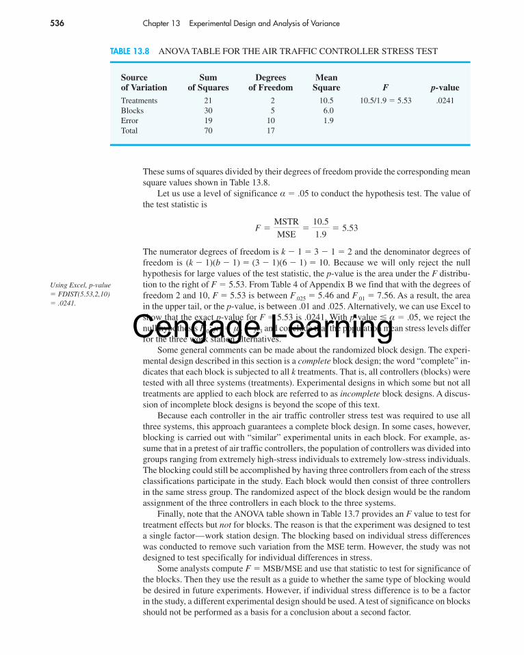
536 Chapter 13 Experimental Design and Analysis of Variance
These sums of squares divided by their degrees of freedom provide the corresponding meansquare values shown in Table 13.8.
Let us use a level of significance α � .05 to conduct the hypothesis test. The value ofthe test statistic is
The numerator degrees of freedom is k � 1 � 3 � 1 � 2 and the denominator degrees offreedom is (k � 1)(b � 1) � (3 � 1)(6 � 1) � 10. Because we will only reject the nullhypothesis for large values of the test statistic, the p-value is the area under the F distribu-tion to the right of F � 5.53. From Table 4 of Appendix B we find that with the degrees offreedom 2 and 10, F � 5.53 is between F.025 � 5.46 and F.01 � 7.56. As a result, the areain the upper tail, or the p-value, is between .01 and .025. Alternatively, we can use Excel toshow that the exact p-value for F � 5.53 is .0241. With p-value � α � .05, we reject thenull hypothesis H0: µ1 � µ2 � µ3 and conclude that the population mean stress levels differfor the three work station alternatives.
Some general comments can be made about the randomized block design. The experi-mental design described in this section is a complete block design; the word “complete” in-dicates that each block is subjected to all k treatments. That is, all controllers (blocks) weretested with all three systems (treatments). Experimental designs in which some but not alltreatments are applied to each block are referred to as incomplete block designs. A discus-sion of incomplete block designs is beyond the scope of this text.
Because each controller in the air traffic controller stress test was required to use allthree systems, this approach guarantees a complete block design. In some cases, however,blocking is carried out with “similar” experimental units in each block. For example, as-sume that in a pretest of air traffic controllers, the population of controllers was divided intogroups ranging from extremely high-stress individuals to extremely low-stress individuals.The blocking could still be accomplished by having three controllers from each of the stressclassifications participate in the study. Each block would then consist of three controllersin the same stress group. The randomized aspect of the block design would be the randomassignment of the three controllers in each block to the three systems.
Finally, note that the ANOVA table shown in Table 13.7 provides an F value to test fortreatment effects but not for blocks. The reason is that the experiment was designed to testa single factor—work station design. The blocking based on individual stress differenceswas conducted to remove such variation from the MSE term. However, the study was notdesigned to test specifically for individual differences in stress.
Some analysts compute F � MSB/MSE and use that statistic to test for significance ofthe blocks. Then they use the result as a guide to whether the same type of blocking wouldbe desired in future experiments. However, if individual stress difference is to be a factorin the study, a different experimental design should be used. A test of significance on blocksshould not be performed as a basis for a conclusion about a second factor.
F �MSTR
MSE�
10.5
1.9� 5.53
Source Sum Degrees Meanof Variation of Squares of Freedom Square F p-valueTreatments 21 2 10.5 10.5/1.9 � 5.53 .0241Blocks 30 5 6.0Error 19 10 1.9Total 70 17
TABLE 13.8 ANOVA TABLE FOR THE AIR TRAFFIC CONTROLLER STRESS TEST
Using Excel, p-value � FDIST(5.53,2,10) � .0241.
56130_13_ch13_p508-560.qxd 2/22/08 11:04 PM Page 536
Cengage Learning
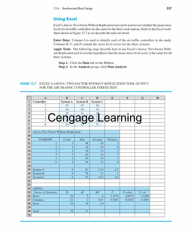
13.4 Randomized Block Design 537
Using ExcelExcel’s Anova: Two-Factor Without Replication tool can be used to test whether the mean stresslevels for air traffic controllers are the same for the three work stations. Refer to the Excel work-sheet shown in Figure 13.7 as we describe the tasks involved.
Enter Data: Column A is used to identify each of the air traffic controllers in the study.Columns B, C, and D contain the stress level scores for the three systems.
Apply Tools: The following steps describe how to use Excel’s Anova: Two-Factor With-out Replication tool to test the hypothesis that the mean stress level score is the same for allthree systems.
Step 1. Click the Data tab on the RibbonStep 2. In the Analysis group, click Data Analysis
FIGURE 13.7 EXCEL’S ANOVA: TWO-FACTOR WITHOUT REPLICATION TOOL OUTPUTFOR THE AIR TRAFFIC CONTROLLER STRESS TEST
A B C D E F G H1 Controller System A System B System C2 1 15 15 183 2 14 14 144 3 10 11 155 4 13 12 176 5 16 13 167 6 13 13 1389 Anova: Two-Factor Without Replication1011 SUMMARY Count Sum Average Variance12 1 3 48 16 313 2 3 42 14 014 3 3 36 12 715 4 3 42 14 716 5 3 45 15 317 6 3 39 13 01819 System A 6 81 13.5 4.320 System B 6 78 13 221 System C 6 93 15.5 3.5222324 ANOVA25 Source of Variation SS df MS F P-value F crit26 Rows 30 5 6 3.1579 0.0574 3.325827 Columns 21 2 10.5 5.5263 0.0242 4.102828 Error 19 10 1.92930 Total 70 1731
56130_13_ch13_p508-560.qxd 2/22/08 11:04 PM Page 537
Cengage Learning
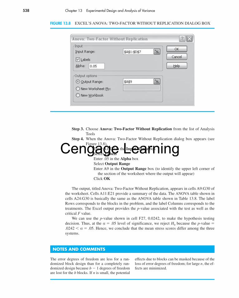
538 Chapter 13 Experimental Design and Analysis of Variance
NOTES AND COMMENTS
The error degrees of freedom are less for a ran-domized block design than for a completely ran-domized design because b � 1 degrees of freedomare lost for the b blocks. If n is small, the potential
effects due to blocks can be masked because of theloss of error degrees of freedom; for large n, the ef-fects are minimized.
Step 3. Choose Anova: Two-Factor Without Replication from the list of AnalysisTools
Step 4. When the Anova: Two-Factor Without Replication dialog box appears (seeFigure 13.8),
Enter A1:D7 in the Input Range boxSelect LabelsEnter .05 in the Alpha boxSelect Output RangeEnter A9 in the Output Range box (to identify the upper left corner of
the section of the worksheet where the output will appear)Click OK
The output, titled Anova: Two-Factor Without Replication, appears in cells A9:G30 ofthe worksheet. Cells A11:E21 provide a summary of the data. The ANOVA table shown incells A24:G30 is basically the same as the ANOVA table shown in Table 13.8. The labelRows corresponds to the blocks in the problem, and the label Columns corresponds to thetreatments. The Excel output provides the p-value associated with the test as well as thecritical F value.
We can use the p-value shown in cell F27, 0.0242, to make the hypothesis testingdecision. Thus, at the α � .05 level of significance, we reject H0 because the p-value �.0242 � α � .05. Hence, we conclude that the mean stress scores differ among the threesystems.
FIGURE 13.8 EXCEL’S ANOVA: TWO-FACTOR WITHOUT REPLICATION DIALOG BOX
56130_13_ch13_p508-560.qxd 2/22/08 11:04 PM Page 538
Cengage Learning

13.4 Randomized Block Design 539
Treatments
A B C
1 10 9 82 12 6 5
Blocks 3 18 15 144 20 18 185 8 7 8
Source Sum Degrees Meanof Variation of Squares of Freedom Square F
Treatments 900 Blocks 400 Error Total 1800
Use α � .05 to test for any significant differences.
22. The following data were obtained for a randomized block design involving five treatmentsand three blocks: SST � 430, SSTR � 310, SSBL � 85. Set up the ANOVA table and testfor any significant differences. Use α � .05.
23. An experiment has been conducted for four treatments with eight blocks. Complete the fol-lowing analysis of variance table.
Use α � .05 to test for any significant differences.
Applications24. An automobile dealer conducted a test to determine if the time in minutes needed to com-
plete a minor engine tune-up depends on whether a computerized engine analyzer or anelectronic analyzer is used. Because tune-up time varies among compact, intermediate, andfull-sized cars, the three types of cars were used as blocks in the experiment. The dataobtained follow.
Use α � .05 to test for any significant differences.25. Prices for vitamins and other health supplements increased over the past several years, and
the prices charged by different retail outlets often vary a great deal. The following datashow the prices for 13 products at four retail outlets in Rochester, New York [RochesterDemocrat and Chronicle, February 13, 2005].
Analyzer
Computerized Electronic
Compact 50 42Car Intermediate 55 44
Full-sized 63 46
Exercises
Methods21. Consider the experimental results for the following randomized block design. Make the
calculations necessary to set up the analysis of variance table.testSELF
56130_13_ch13_p508-560.qxd 2/22/08 11:04 PM Page 539
Cengage Learning
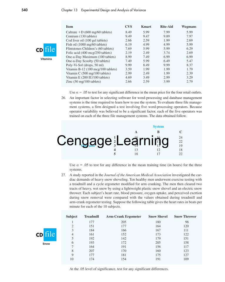
540 Chapter 13 Experimental Design and Analysis of Variance
Subject Treadmill Arm-Crank Ergometer Snow Shovel Snow Thrower
1 177 205 180 982 151 177 164 1203 184 166 167 1114 161 152 173 1225 192 142 179 1516 193 172 205 1587 164 191 156 1178 207 170 160 1239 177 181 175 127
10 174 154 191 109
fileCDSnow
System
A B C
1 16 16 242 19 17 22
Operator 3 14 13 194 13 12 185 18 17 22
Item CVS Kmart Rite-Aid Wegmans
Caltrate �D (600 mg/60 tablets) 8.49 5.99 7.99 5.99Centrum (130 tablets) 9.49 9.47 9.89 7.97Cod liver oil (100 gel tablets) 2.66 2.59 1.99 2.69Fish oil (1000 mg/60 tablets) 6.19 4.99 4.99 5.99Flintstones Children’s (60 tablets) 7.69 5.99 5.99 6.29Folic acid (400 mcg/250 tablets) 2.19 2.49 3.74 2.69One-a-Day Maximum (100 tablets) 8.99 7.49 6.99 6.99One-a-Day Scooby (50 tablets) 7.49 5.99 6.49 5.47Poly-Vi-Sol (drops, 50 ml) 9.99 8.49 9.99 8.37Vitamin B-12 (100 mcg/100 tablets) 3.59 1.99 1.99 1.79Vitamin C (500 mg/100 tablets) 2.99 2.49 1.99 2.39Vitamin E (200 IU/100 tablets) 4.69 3.49 2.99 3.29Zinc (50 mg/100 tablets) 2.66 2.59 3.99 2.79
fileCDVitamins
Use α � .05 to test for any significant difference in the mean price for the four retail outlets.
26. An important factor in selecting software for word-processing and database managementsystems is the time required to learn how to use the system. To evaluate three file manage-ment systems, a firm designed a test involving five word-processing operators. Becauseoperator variability was believed to be a significant factor, each of the five operators wastrained on each of the three file management systems. The data obtained follow.
Use α � .05 to test for any difference in the mean training time (in hours) for the threesystems.
27. A study reported in the Journal of the American Medical Association investigated the car-diac demands of heavy snow shoveling. Ten healthy men underwent exercise testing witha treadmill and a cycle ergometer modified for arm cranking. The men then cleared twotracts of heavy, wet snow by using a lightweight plastic snow shovel and an electric snowthrower. Each subject’s heart rate, blood pressure, oxygen uptake, and perceived exertionduring snow removal were compared with the values obtained during treadmill andarm-crank ergometer testing. Suppose the following table gives the heart rates in beats perminute for each of the 10 subjects.
At the .05 level of significance, test for any significant differences.
56130_13_ch13_p508-560.qxd 2/22/08 11:04 PM Page 540
Cengage Learning

13.5 Factorial Experiment 541
13.5 Factorial ExperimentThe experimental designs we have considered thus far enable us to draw statistical conclusionsabout one factor. However, in some experiments we want to draw conclusions about more thanone variable or factor. A factorial experiment is an experimental design that allows simulta-neous conclusions about two or more factors. The term factorial is used because the experi-mental conditions include all possible combinations of the factors. For example, for a levels offactor A and b levels of factor B, the experiment will involve collecting data on ab treatmentcombinations. In this section we will show the analysis for a two-factor factorial experiment.The basic approach can be extended to experiments involving more than two factors.
As an illustration of a two-factor factorial experiment, we will consider a study involvingthe Graduate Management Admissions Test (GMAT), a standardized test used by graduateschools of business to evaluate an applicant’s ability to pursue a graduate program in that field.Scores on the GMAT range from 200 to 800, with higher scores implying higher aptitude.
In an attempt to improve students’ performance on the GMAT exam, a major Texas uni-versity is considering offering the following three GMAT preparation programs.
1. A three-hour review session covering the types of questions generally asked on theGMAT.
2. A one-day program covering relevant exam material, along with the taking andgrading of a sample exam.
3. An intensive 10-week course involving the identification of each student’s weak-nesses and the setting up of individualized programs for improvement.
Hence, one factor in this study is the GMAT preparation program, which has three treat-ments: three-hour review, one-day program, and 10-week course. Before selecting thepreparation program to adopt, further study will be conducted to determine how the pro-posed programs affect GMAT scores.
The GMAT is usually taken by students from three colleges: the College of Business,the College of Engineering, and the College of Arts and Sciences. Therefore, a second factorof interest in the experiment is whether a student’s undergraduate college affects the GMATscore. This second factor, undergraduate college, also has three treatments: business, engi-neering, and arts and sciences. The factorial design for this experiment with three treatmentscorresponding to factor A, the preparation program, and three treatments corresponding tofactor B, the undergraduate college, will have a total of 3 3 � 9 treatment combinations.These treatment combinations or experimental conditions are summarized in Table 13.9.
Assume that a sample of two students will be selected corresponding to each of the ninetreatment combinations shown in Table 13.9: two business students will take the three-hourreview, two will take the one-day program, and two will take the 10-week course. In addi-tion, two engineering students and two arts and sciences students will take each of the threepreparation programs. In experimental design terminology, the sample size of two for eachtreatment combination indicates that we have two replications. Additional replications
Factor B: College
Business Engineering Arts and SciencesFactor A: Three-hour review 1 2 3Preparation One-day program 4 5 6Program 10-week course 7 8 9
TABLE 13.9 NINE TREATMENT COMBINATIONS FOR THE TWO-FACTOR GMAT EXPERIMENT
56130_13_ch13_p508-560.qxd 2/22/08 11:04 PM Page 541
Cengage Learning
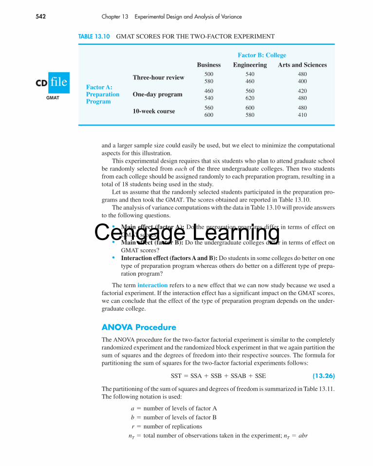
542 Chapter 13 Experimental Design and Analysis of Variance
and a larger sample size could easily be used, but we elect to minimize the computationalaspects for this illustration.
This experimental design requires that six students who plan to attend graduate schoolbe randomly selected from each of the three undergraduate colleges. Then two studentsfrom each college should be assigned randomly to each preparation program, resulting in atotal of 18 students being used in the study.
Let us assume that the randomly selected students participated in the preparation pro-grams and then took the GMAT. The scores obtained are reported in Table 13.10.
The analysis of variance computations with the data in Table 13.10 will provide answersto the following questions.
• Main effect (factor A): Do the preparation programs differ in terms of effect onGMAT scores?
• Main effect (factor B): Do the undergraduate colleges differ in terms of effect onGMAT scores?
• Interaction effect (factors A and B): Do students in some colleges do better on onetype of preparation program whereas others do better on a different type of prepa-ration program?
The term interaction refers to a new effect that we can now study because we used afactorial experiment. If the interaction effect has a significant impact on the GMAT scores,we can conclude that the effect of the type of preparation program depends on the under-graduate college.
ANOVA ProcedureThe ANOVA procedure for the two-factor factorial experiment is similar to the completelyrandomized experiment and the randomized block experiment in that we again partition thesum of squares and the degrees of freedom into their respective sources. The formula forpartitioning the sum of squares for the two-factor factorial experiments follows:
(13.26)
The partitioning of the sum of squares and degrees of freedom is summarized in Table 13.11.The following notation is used:
a �
b �
r �
nT �
number of levels of factor A
number of levels of factor B
number of replications
total number of observations taken in the experiment; nT � abr
SST � SSA � SSB � SSAB � SSE
Factor B: College
Business Engineering Arts and Sciences
Three-hour review 500 540 480
Factor A:580 460 400
Preparation One-day program 460 560 420
Program 540 620 480
10-week course 560 600 480600 580 410
TABLE 13.10 GMAT SCORES FOR THE TWO-FACTOR EXPERIMENT
fileCDGMAT
56130_13_ch13_p508-560.qxd 2/22/08 11:04 PM Page 542
Cengage Learning
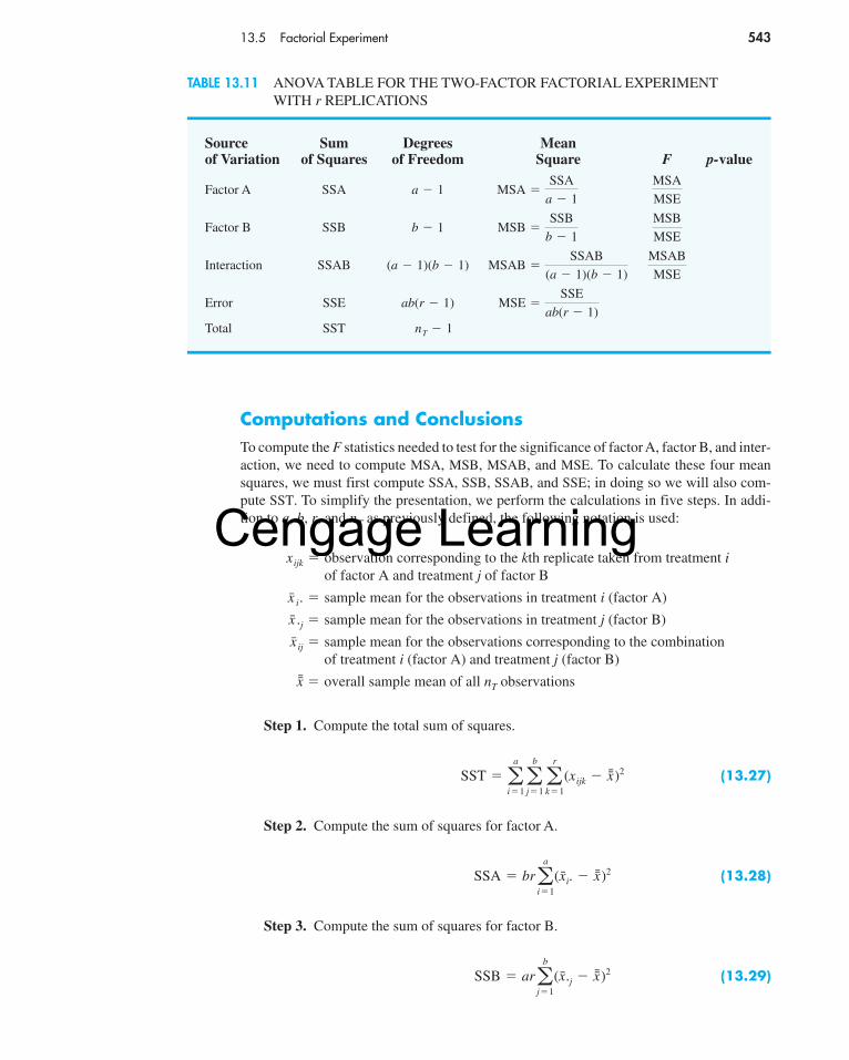
13.5 Factorial Experiment 543
Computations and ConclusionsTo compute the F statistics needed to test for the significance of factor A, factor B, and inter-action, we need to compute MSA, MSB, MSAB, and MSE. To calculate these four meansquares, we must first compute SSA, SSB, SSAB, and SSE; in doing so we will also com-pute SST. To simplify the presentation, we perform the calculations in five steps. In addi-tion to a, b, r, and nT as previously defined, the following notation is used:
Step 1. Compute the total sum of squares.
(13.27)
Step 2. Compute the sum of squares for factor A.
(13.28)
Step 3. Compute the sum of squares for factor B.
(13.29)SSB � ar �b
j�1
(x̄.j � x̄̄ )2
SSA � br �a
i�1
(x̄i. � x̄̄ )2
SST � �a
i�1
�b
j�1
�r
k�1
(xijk � x̄̄ )2
x̄̄ � overall sample mean of all nT observations
x̄ ij �
sample mean for the observations corresponding to the combinationof treatment i (factor A) and treatment j (factor B)
x̄ .j � sample mean for the observations in treatment j (factor B)
x̄ i. � sample mean for the observations in treatment i (factor A)
xijk �
observation corresponding to the kth replicate taken from treatment iof factor A and treatment j of factor B
Source Sum Degrees Meanof Variation of Squares of Freedom Square F p-value
Factor A SSA
Factor B SSB
Interaction SSAB
Error SSE
Total SST nT � 1
MSE �SSE
ab(r � 1)ab(r � 1)
MSAB
MSEMSAB �
SSAB
(a � 1)(b � 1)(a � 1)(b � 1)
MSB
MSEMSB �
SSB
b � 1b � 1
MSA
MSEMSA �
SSA
a � 1a � 1
TABLE 13.11 ANOVA TABLE FOR THE TWO-FACTOR FACTORIAL EXPERIMENTWITH r REPLICATIONS
56130_13_ch13_p508-560.qxd 2/22/08 11:04 PM Page 543
Cengage Learning

544 Chapter 13 Experimental Design and Analysis of Variance
Step 4. Compute the sum of squares for interaction.
(13.30)
Step 5. Compute the sum of squares due to error.
(13.31)
Table 13.12 reports the data collected in the experiment and the various sums thatwill help us with the sum of squares computations. Using equations (13.27) through(13.31), we calculate the following sums of squares for the GMAT two-factor factorialexperiment.
Step 1. SST � (500 � 515)2 � (580 � 515)2 � (540 � 515)2 � . . . �(410 � 515)2 � 82,450
Step 2. SSA � (3)(2)[(493.33 � 515)2 � (513.33 � 515)2 �(538.33 � 515)2] � 6100
Step 3. SSB � (3)(2)[(540 � 515)2 � (560 � 515)2 � (445 � 515)2] � 45,300
Step 4. SSAB � 2[(540 � 493.33 � 540 � 515)2 � (500 � 493.33 �560 � 515)2 � . . . � (445 � 538.33 � 445 � 515)2] � 11,200
Step 5. SSE � 82,450 � 6100 � 45,300 � 11,200 � 19,850
These sums of squares divided by their corresponding degrees of freedom provide the fol-lowing mean square values for testing the two main effects (preparation program and un-dergraduate college) and interaction effect.
Factor A:
Factor B:
Interaction:
Error:
Let us use a level of significance of α � .05 to conduct the hypothesis tests for the two-factor GMAT study. The F ratio used to test for differences among preparation programs(factor A) is F � MSA/MSE � 3050/2205.5556 � 1.3829. We can use Excel to show thatthe p-value corresponding to F � 1.3829 is .2994. Because the p-value � α � .05, wecannot reject the null hypothesis and must conclude that there is no significant differenceamong the three preparation programs. However, for the undergraduate college (factor B)effect, the p-value corresponding to F � MSB/MSE � 22,650/2205.5556 � 10.2695 is.0048. Hence, the analysis of variance results enable us to conclude that the GMAT testscores do differ among the three undergraduate colleges; that is, the three undergraduatecolleges do not provide the same preparation for performance on the GMAT. Finally, theinteraction F value of F � MSAB/MSE � 2800/2205.5556 � 1.2695 and its correspond-ing p-value of .3503 mean we cannot identify a significant interaction effect. Therefore,we have no reason to believe that the three preparation programs differ in their ability to
MSE �SSE
ab(r � 1)�
19,850
(3)(3)(2 � 1)� 2205.5556
MSAB �SSAB
(a � 1)(b � 1)�
11,200
(3 � 1)(3 � 1)� 2800
MSB �SSB
b � 1�
45,300
3 � 1� 22,650
MSA �SSA
a � 1�
6100
3 � 1� 3050
SSE � SST � SSA � SSB � SSAB
SSAB � r �a
i�1
�b
j�1
(x̄ ij � x̄i. � x̄.j � x̄̄ )2
Excel’s FDIST functionmakes it easy to computethe p-value for each Fvalue. For example, forfactor A, p-value � FDIST(1.3829,2,9) � .2994.
56130_13_ch13_p508-560.qxd 2/22/08 11:04 PM Page 544
Cengage Learning
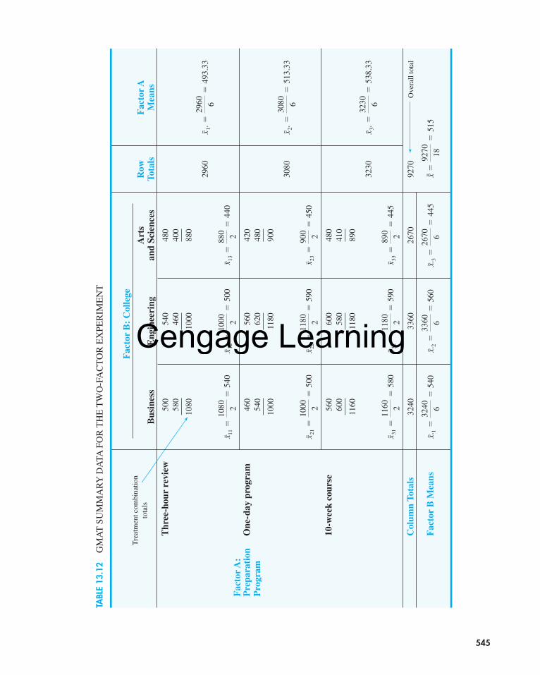
Fac
tor
B:
Col
lege
Art
sR
owF
acto
rA
Bus
ines
sE
ngin
eeri
ngan
d Sc
ienc
esTo
tals
Mea
ns
Thr
ee-h
our
revi
ew50
054
048
058
046
040
0
1080
1000
880
2960
Fac
tor
A:
Pre
para
tion
One
-day
pro
gram
460
560
420
Pro
gram
540
620
480
1000
1180
900
3080
10-w
eek
cour
se56
060
048
060
058
041
0
1160
1180
890
3230
Col
umn
Tota
ls32
4033
6026
7092
70
Fac
tor
B M
eans
x̄̄�
9270 18
�51
5x̄.
3�
2670 6
�44
5x̄.
2�
3360 6
�56
0x̄.
1�
3240 6
�54
0
x̄ 33
�89
0 2�
445
x̄ 32
�11
80 2�
590
x̄ 31
�11
60 2�
580
x̄ 3.�
3230 6
�53
8.33
x̄ 23
�90
0 2�
450
x̄ 22
�11
80 2�
590
x̄ 21
�10
00 2�
500
x̄ 2.�
3080 6
�51
3.33
x̄ 13
�88
0 2�
440
x̄ 12
�10
00 2�
500
x̄ 11
�10
80 2�
540
x̄ 1.�
2960 6
�49
3.33
TABL
E 13
.12
GM
AT
SUM
MA
RY
DA
TAFO
R T
HE
TW
O-F
AC
TO
R E
XPE
RIM
EN
T
Tre
atm
ent c
ombi
natio
nto
tals
Ove
rall
tota
l
545
56130_13_ch13_p508-560.qxd 2/22/08 11:04 PM Page 545
Cengage Learning

546 Chapter 13 Experimental Design and Analysis of Variance
Source Sum Degrees Meanof Variation of Squares of Freedom Square F p-valueFactor A 6,100 2 3,050 3,050/2206 � 1.3829 .2994Factor B 45,300 2 22,650 22,650/2206 � 10.2695 .0048Interaction 11,200 4 2,800 2,800/2206 � 1.2695 .3503Error 19,850 9 2,206Total 82,450 17
TABLE 13.13 ANOVA TABLE FOR THE TWO-FACTOR GMAT STUDY
prepare students from the different colleges for the GMAT. The ANOVA table shown inTable 13.13 provides a summary of these results for the two-factor GMAT study.
Undergraduate college was found to be a significant factor. Checking the calculationsin Table 13.12, we see that the sample means are: business students .1 � 540, engineer-ing students .2 � 560, and arts and sciences students .3 � 445. Tests on individual treat-ment means can be conducted; yet after reviewing the three sample means, we wouldanticipate no difference in preparation for business and engineering graduates. However,the arts and sciences students appear to be significantly less prepared for the GMAT thanstudents in the other colleges. Perhaps this observation will lead the university to con-sider other options for assisting these students in preparing for graduate managementadmission tests.
Using ExcelExcel’s Anova: Two-Factor With Replication tool can be used to analyze the data for thetwo-factor GMAT experiment. Refer to the Excel worksheet shown in Figure 13.9 as wedescribe the tasks involved.
Enter Data: Column A is used to identify each of the preparation programs (factor A) inthe study. Column B contains the GMAT scores for the Business students, column C con-tains the GMAT scores for the Engineering students, and column D contains the GMATscores for the Arts and Sciences students.
Apply Tools: The following steps describe how Excel’s Anova: Two-Factor With Repli-cation tool can be used to analyze the data for the two-factor GMAT experiment.
Step 1. Click the Data tab on the RibbonStep 2. In the Analysis group, click Data AnalysisStep 3. Choose Anova: Two-Factor With Replication from the list of Analysis ToolsStep 4. When the Anova: Two-Factor With Replication dialog box appears (see Fig-
ure 13.10),Enter A1:D7 in the Input Range boxEnter 2 in the Rows per sample boxEnter .05 in the Alpha boxSelect Output RangeEnter A9 in the Output Range box (to identify the upper left corner of
the section of the worksheet where the output will appear)Click OK
The output, titled Anova: Two-Factor With Replication, appears in cells A9:G44 of the worksheet. Cells A11:E34 provide a summary of the data. The ANOVA table, shown in
x̄x̄x̄
56130_13_ch13_p508-560.qxd 2/22/08 11:04 PM Page 546
Cengage Learning

13.5 Factorial Experiment 547
FIGURE 13.9 EXCEL’S ANOVA: TWO-FACTOR WITH REPLICATION TOOL OUTPUTFOR THE GMAT EXPERIMENT
A B C D E F G H1 Business Engineering Arts and Sciences2 3-hour review 500 540 4803 580 460 4004 1-day program 460 560 4205 540 620 4806 10-week course 560 600 4807 600 580 41089 Anova: Two-Factor With Replication
1011 SUMMARY Business Engineering Arts and Sciences Total12 3-hour review13 Count 2 2 2 614 Sum 1080 1000 880 296015 Average 540 500 440 493.333316 Variance 3200 3200 3200 3946.6671718 1-day program19 Count 2 2 2 620 Sum 1000 1180 900 308021 Average 500 590 450 513.333322 Variance 3200 1800 1800 5386.6672324 10-week course25 Count 2 2 2 626 Sum 1160 1180 890 323027 Average 580 590 445 538.333328 Variance 800 200 2450 5936.6672930 Total31 Count 6 6 632 Sum 3240 3360 267033 Average 540 560 44534 Variance 2720 3200 1510353637 ANOVA38 Source of Variation SS df MS F P-value F crit39 Sample 6100 2 3050 1.3829 0.2994 4.256540 Columns 45300 2 22650 10.2695 0.0048 4.256541 Interaction 11200 4 2800 1.2695 0.3503 3.633142 Within 19850 9 2205.55564344 Total 82450 1745
cells A37:G44, is basically the same as the ANOVA table shown in Table 13.13. The labelSample corresponds to factor A, the label Columns corresponds to factor B, and the labelWithin corresponds to error. The Excel output provides the p-value associated with each F test as well as the critical F values.
We can use the p-value of .2994 in cell F39 to make the hypothesis testing decision forfactor A (Preparation Program). At the α � .05 level of significance, we cannot reject H0
because the p-value � .2994 � α � .05. We can make the hypothesis testing decision
56130_13_ch13_p508-560.qxd 2/22/08 11:04 PM Page 547
Cengage Learning

548 Chapter 13 Experimental Design and Analysis of Variance
Factor B
Level 1 Level 2 Level 3
135 90 75Level 1 165 66 93
Factor A125 127 120
Level 2 95 105 136
testSELF
Test for any significant main effects and any interaction. Use α � .05.
29. The calculations for a factorial experiment involving four levels of factor A, three levelsof factor B, and three replications resulted in the following data: SST � 280, SSA � 26,SSB � 23, SSAB � 175. Set up the ANOVA table and test for any significant main effectsand any interaction effect. Use α � .05.
Applications30. A mail-order catalog firm designed a factorial experiment to test the effect of the size of
a magazine advertisement and the advertisement design on the number of catalogrequests received (data in thousands). Three advertising designs and two different-sizeadvertisements were considered. The data obtained follow. Use the ANOVA procedure for
for factor B (College) by using the p-value of 0.0048 shown in cell F40. At the α � .05 level of significance, we reject H0 because the p-value � .0048 � α � .05. Finally, theinteraction p-value of 0.3503 in cell F41 means that we cannot identify a significant inter-action effect.
Exercises
Methods28. A factorial experiment involving two levels of factor A and three levels of factor B resulted
in the following data.
FIGURE 13.10 EXCEL’S ANOVA: TWO-FACTOR WITH REPLICATION DIALOG BOX
56130_13_ch13_p508-560.qxd 2/22/08 11:04 PM Page 548
Cengage Learning

13.5 Factorial Experiment 549
factorial designs to test for any significant effects due to type of design, size of advertise-ment, or interaction. Use α � .05.
Type of Ride
Roller Coaster Screaming Demon Log Flume
Method 1 41 52 5043 44 46
Method 2 49 50 4851 46 44
Weekly Salary ($) Occupation Gender
872 Financial Manager Male859 Financial Manager Male
1028 Financial Manager Male1117 Financial Manager Male1019 Financial Manager Male519 Financial Manager Female702 Financial Manager Female805 Financial Manager Female558 Financial Manager Female591 Financial Manager Female747 Computer Programmer Male766 Computer Programmer Male901 Computer Programmer Male690 Computer Programmer Male
(continued)
fileCDSalaries
Size of Advertisement
Small Large
A 8 1212 8
Design B 22 2614 30
C 10 1818 14
31. An amusement park studied methods for decreasing the waiting time (minutes) for rides byloading and unloading riders more efficiently. Two alternative loading/unloading methodshave been proposed. To account for potential differences due to the type of ride and thepossible interaction between the method of loading and unloading and the type of ride, a fac-torial experiment was designed. Use the following data to test for any significant effect dueto the loading and unloading method, the type of ride, and interaction. Use α � .05.
32. The U.S. Bureau of Labor Statistics collects information on the earnings of men andwomen for different occupations. Suppose that a reporter for The Tampa Tribune wantedto investigate whether there were any differences between the weekly salaries of men and women employed as financial managers, computer programmers, and pharmacists. Asample of five men and women was selected from each of the three occupations, and theweekly salary for each individual in the sample was recorded. The data obtained follow.
56130_13_ch13_p508-560.qxd 2/22/08 11:04 PM Page 549
Cengage Learning
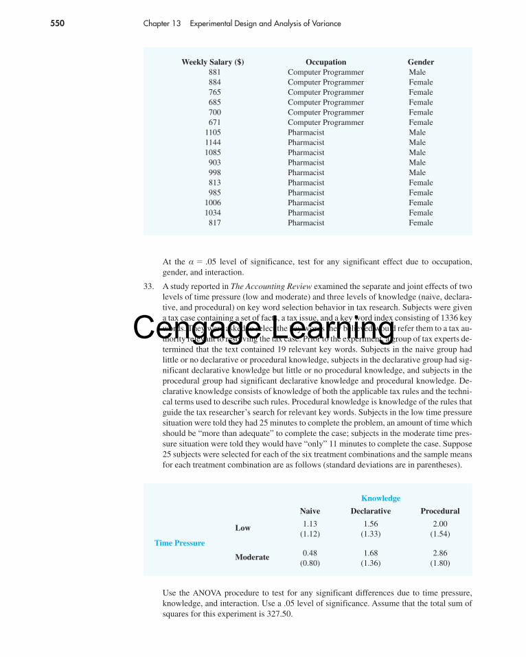
550 Chapter 13 Experimental Design and Analysis of Variance
At the α � .05 level of significance, test for any significant effect due to occupation,gender, and interaction.
33. A study reported in The Accounting Review examined the separate and joint effects of twolevels of time pressure (low and moderate) and three levels of knowledge (naive, declara-tive, and procedural) on key word selection behavior in tax research. Subjects were givena tax case containing a set of facts, a tax issue, and a key word index consisting of 1336 keywords. They were asked to select the key words they believed would refer them to a tax au-thority relevant to resolving the tax case. Prior to the experiment, a group of tax experts de-termined that the text contained 19 relevant key words. Subjects in the naive group hadlittle or no declarative or procedural knowledge, subjects in the declarative group had sig-nificant declarative knowledge but little or no procedural knowledge, and subjects in theprocedural group had significant declarative knowledge and procedural knowledge. De-clarative knowledge consists of knowledge of both the applicable tax rules and the techni-cal terms used to describe such rules. Procedural knowledge is knowledge of the rules thatguide the tax researcher’s search for relevant key words. Subjects in the low time pressuresituation were told they had 25 minutes to complete the problem, an amount of time whichshould be “more than adequate” to complete the case; subjects in the moderate time pres-sure situation were told they would have “only” 11 minutes to complete the case. Suppose25 subjects were selected for each of the six treatment combinations and the sample meansfor each treatment combination are as follows (standard deviations are in parentheses).
Knowledge
Naive Declarative Procedural
Low 1.13 1.56 2.00(1.12) (1.33) (1.54)
Time Pressure
Moderate 0.48 1.68 2.86(0.80) (1.36) (1.80)
Weekly Salary ($) Occupation Gender881 Computer Programmer Male884 Computer Programmer Female765 Computer Programmer Female685 Computer Programmer Female700 Computer Programmer Female671 Computer Programmer Female
1105 Pharmacist Male1144 Pharmacist Male1085 Pharmacist Male903 Pharmacist Male998 Pharmacist Male813 Pharmacist Female985 Pharmacist Female
1006 Pharmacist Female1034 Pharmacist Female817 Pharmacist Female
Use the ANOVA procedure to test for any significant differences due to time pressure,knowledge, and interaction. Use a .05 level of significance. Assume that the total sum ofsquares for this experiment is 327.50.
56130_13_ch13_p508-560.qxd 2/22/08 11:04 PM Page 550
Cengage Learning

Glossary 551
Summary
In this chapter we introduced the completely randomized design, the randomized block de-sign, and the two-factor factorial experiment. The completely randomized design and therandomized block design are used to draw conclusions about differences in the means ofa single factor. The primary purpose of blocking in the randomized block design is toremove extraneous sources of variation from the error term. Such blocking provides abetter estimate of the true error variance and a better test to determine whether the populationor treatment means of the factor differ significantly.
We showed how analysis of variance can be used to test for differences among meansof several populations or treatments. The basis for the statistical tests used in analysis ofvariance and experimental design is the development of two independent estimates of thepopulation variance σ 2. In the single-factor case, one estimator is based on the variation be-tween the treatments; this estimator provides an unbiased estimate of σ 2 only if the meansµ1, µ2, . . . , µk are all equal. A second estimator of σ 2 is based on the variation of the ob-servations within each sample; this estimator will always provide an unbiased estimate ofσ 2. By computing the ratio of these two estimators (the F statistic) we developed a rejec-tion rule for determining whether to reject the null hypothesis that the population or treat-ment means are equal. In all the experimental designs considered, the partitioning of thesum of squares and degrees of freedom into their various sources enabled us to compute theappropriate values for the analysis of variance calculations and tests. We also showed howFisher’s LSD procedure and the Bonferroni adjustment can be used to perform pairwisecomparisons to determine which means are different.
Glossary
Factor Another word for the independent variable of interest.Treatments Different levels of a factor.Single-factor experiment An experiment involving only one factor with k populations ortreatments.Response variable Another word for the dependent variable of interest.Experimental units The objects of interest in the experiment.Completely randomized design An experimental design in which the treatments arerandomly assigned to the experimental units.ANOVA table A table used to summarize the analysis of variance computations and results.It contains columns showing the source of variation, the sum of squares, the degrees of free-dom, the mean square, the F value(s), and the p-value(s).Partitioning The process of allocating the total sum of squares and degrees of freedom tothe various components.Multiple comparison procedures Statistical procedures that can be used to conductstatistical comparisons between pairs of population means.Comparisonwise Type I error rate The probability of a Type I error associated with asingle pairwise comparison.Experimentwise Type I error rate The probability of making a Type I error on at least oneof several pairwise comparisons.Blocking The process of using the same or similar experimental units for all treatments.The purpose of blocking is to remove a source of variation from the error term and henceprovide a more powerful test for a difference in population or treatment means.Randomized block design An experimental design employing blocking.Factorial experiment An experimental design that allows simultaneous conclusions abouttwo or more factors.
56130_13_ch13_p508-560.qxd 2/22/08 11:04 PM Page 551
Cengage Learning

552 Chapter 13 Experimental Design and Analysis of Variance
Replications The number of times each experimental condition is repeated in an experiment.Interaction The effect produced when the levels of one factor interact with the levels ofanother factor in influencing the response variable.
Key Formulas
Completely Randomized Design
Sample Mean for Treatment j
(13.1)
Sample Variance for Treatment j
(13.2)
Overall Sample Mean
(13.3)
(13.4)
Mean Square Due to Treatments
(13.7)
Sum of Squares Due to Treatments
(13.8)
Mean Square Due to Error
(13.10)
Sum of Squares Due to Error
(13.11)
Test Statistic for the Equality of k Population Means
(13.12)F �MSTR
MSE
SSE � �k
j�1
(nj � 1)s2j
MSE �SSE
nT � k
SSTR � �k
j�1
nj (x̄ j � x̄̄
)2
MSTR �SSTR
k � 1
nT � n1 � n2 � . . . � nk
x̄̄ ��
k
j�1
�nj
i�1
xij
nT
s2j �
�nj
i�1
(xij � x̄ j)
2
nj � 1
x̄ j ��nj
i�1
xij
nj
56130_13_ch13_p508-560.qxd 2/22/08 11:04 PM Page 552
Cengage Learning

Key Formulas 553
Total Sum of Squares
(13.13)
Partitioning of Sum of Squares
(13.14)
Multiple Comparison ProceduresTest Statistic for Fisher’s LSD Procedure
(13.16)
Fisher’s LSD
(13.17)
Randomized Block DesignTotal Sum of Squares
(13.22)
Sum of Squares Due to Treatments
(13.23)
Sum of Squares Due to Blocks
(13.24)
Sum of Squares Due to Error
(13.25)
Factorial ExperimentTotal Sum of Squares
(13.27)
Sum of Squares for Factor A
(13.28)SSA � br �a
i�1
(x̄ i. � x̄̄ )2
SST � �a
i�1
�b
j�1
�r
k�1
(xijk � x̄̄ )2
SSE � SST � SSTR � SSBL
SSBL � k �b
i�1
(x̄ i. � x̄̄ )2
SSTR � b �k
j�1
(x̄.j � x̄̄ )2
SST � �b
i�1
�k
j�1
(xij � x̄̄ )2
LSD � tα/2�MSE�1ni
�1nj�
t �x̄i � x̄j
�MSE�1ni
�1nj�
SST � SSTR � SSE
SST � �k
j�1
�nj
i�1
(xij � x̄̄)2
56130_13_ch13_p508-560.qxd 2/22/08 11:04 PM Page 553
Cengage Learning
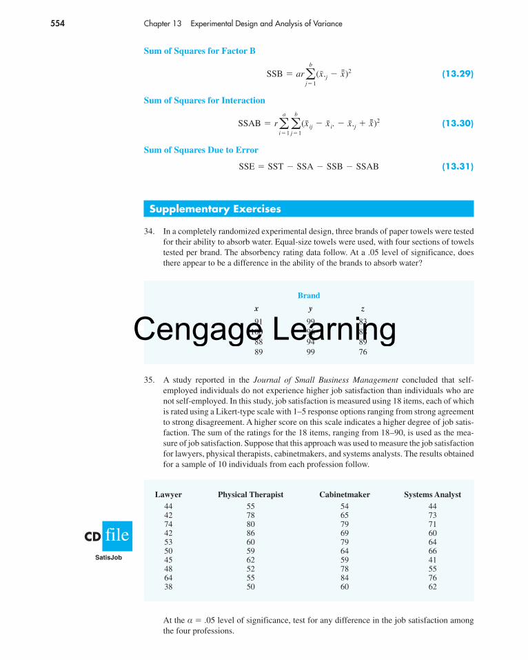
554 Chapter 13 Experimental Design and Analysis of Variance
Sum of Squares for Factor B
(13.29)
Sum of Squares for Interaction
(13.30)
Sum of Squares Due to Error
(13.31)
Supplementary Exercises
34. In a completely randomized experimental design, three brands of paper towels were testedfor their ability to absorb water. Equal-size towels were used, with four sections of towelstested per brand. The absorbency rating data follow. At a .05 level of significance, doesthere appear to be a difference in the ability of the brands to absorb water?
SSE � SST � SSA � SSB � SSAB
SSAB � r �a
i�1
�b
j�1
(x̄ ij � x̄ i. � x̄.j � x̄̄ )2
SSB � ar �b
j�1
(x̄.j � x̄̄ )2
Lawyer Physical Therapist Cabinetmaker Systems Analyst44 55 54 4442 78 65 7374 80 79 7142 86 69 6053 60 79 6450 59 64 6645 62 59 4148 52 78 5564 55 84 7638 50 60 62
fileCDSatisJob
35. A study reported in the Journal of Small Business Management concluded that self-employed individuals do not experience higher job satisfaction than individuals who arenot self-employed. In this study, job satisfaction is measured using 18 items, each of whichis rated using a Likert-type scale with 1–5 response options ranging from strong agreementto strong disagreement. A higher score on this scale indicates a higher degree of job satis-faction. The sum of the ratings for the 18 items, ranging from 18–90, is used as the mea-sure of job satisfaction. Suppose that this approach was used to measure the job satisfactionfor lawyers, physical therapists, cabinetmakers, and systems analysts. The results obtainedfor a sample of 10 individuals from each profession follow.
Brand
x y z
91 99 83100 96 8888 94 8989 99 76
At the α � .05 level of significance, test for any difference in the job satisfaction amongthe four professions.
56130_13_ch13_p508-560.qxd 2/22/08 11:04 PM Page 554
Cengage Learning

Supplementary Exercises 555
36. Money magazine reports percentage returns and expense ratios for stock and bond funds.The following data are the expense ratios for 10 midcap stock funds, 10 small-cap stockfunds, 10 hybrid stock funds, and 10 specialty stock funds (Money, March 2003).
Computers Construction Engineering
Job Salary Job Salary Job Salary
Data Mgr. 94 Administrator 55 Aeronautical 75Mfg. Mgr. 90 Architect 53 Agricultural 70Programmer 63 Architect Mgr. 77 Chemical 88Project Mgr. 84 Const. Mgr. 60 Civil 77Software Dev. 73 Foreperson 41 Electrical 89Sr. Design 75 Interior Design 54 Mechanical 85Staff Systems 94 Landscape Architect 51 Mining 96Systems Analyst 77 Sr. Estimator 64 Nuclear 105
fileCDJobSalary
Method
A B C
97 93 9973 100 9493 93 87
100 55 6673 77 5991 91 75
100 85 8486 73 7292 90 8895 83 86
fileCDAssembly
Use α � .05 to test for any significant difference in the mean expense ratio among the fourtypes of stock funds.
37. Business 2.0’s first annual employment survey provided data showing the typical annualsalary for 97 different jobs. The following data show the annual salary for 30 different jobsin three fields: computer software and hardware, construction, and engineering (Business2.0, March 2003).
Use α � .05 to test for any significant difference in the mean annual salary among the threejob fields.
38. Three different assembly methods have been proposed for a new product. A completelyrandomized experimental design was chosen to determine which assembly method resultsin the greatest number of parts produced per hour, and 30 workers were randomly selectedand assigned to use one of the proposed methods. The number of units produced by eachworker follows.
Midcap Small-Cap Hybrid Specialty
1.2 2.0 2.0 1.61.1 1.2 2.7 2.71.0 1.7 1.8 2.61.2 1.8 1.5 2.51.3 1.5 2.5 1.91.8 2.3 1.0 1.51.4 1.9 0.9 1.61.4 1.3 1.9 2.71.0 1.2 1.4 2.21.4 1.3 0.3 0.7
fileCDFunds
56130_13_ch13_p508-560.qxd 2/22/08 11:04 PM Page 555
Cengage Learning
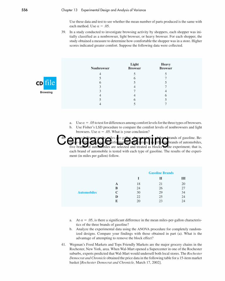
556 Chapter 13 Experimental Design and Analysis of Variance
Use these data and test to see whether the mean number of parts produced is the same witheach method. Use α � .05.
39. In a study conducted to investigate browsing activity by shoppers, each shopper was ini-tially classified as a nonbrowser, light browser, or heavy browser. For each shopper, thestudy obtained a measure to determine how comfortable the shopper was in a store. Higherscores indicated greater comfort. Suppose the following data were collected.
Gasoline Brands
I II III
A 18 21 20B 24 26 27
Automobiles C 30 29 34D 22 25 24E 20 23 24
a. Use α � .05 to test for differences among comfort levels for the three types of browsers.b. Use Fisher’s LSD procedure to compare the comfort levels of nonbrowsers and light
browsers. Use α � .05. What is your conclusion?
40. A research firm tests the miles-per-gallon characteristics of three brands of gasoline. Be-cause of different gasoline performance characteristics in different brands of automobiles,five brands of automobiles are selected and treated as blocks in the experiment; that is,each brand of automobile is tested with each type of gasoline. The results of the experi-ment (in miles per gallon) follow.
a. At α � .05, is there a significant difference in the mean miles-per-gallon characteris-tics of the three brands of gasoline?
b. Analyze the experimental data using the ANOVA procedure for completely random-ized designs. Compare your findings with those obtained in part (a). What is theadvantage of attempting to remove the block effect?
41. Wegman’s Food Markets and Tops Friendly Markets are the major grocery chains in theRochester, New York, area. When Wal-Mart opened a Supercenter in one of the Rochestersuburbs, experts predicted that Wal-Mart would undersell both local stores. The RochesterDemocrat and Chronicle obtained the price data in the following table for a 15-item marketbasket [Rochester Democrat and Chronicle, March 17, 2002].
Light HeavyNonbrowser Browser Browser
4 5 55 6 76 5 53 4 73 7 44 4 65 6 54 5 7
fileCDBrowsing
56130_13_ch13_p508-560.qxd 2/22/08 11:04 PM Page 556
Cengage Learning

Supplementary Exercises 557
Language
Spanish French German
System 1 8 10 1212 14 16
System 2 6 14 1610 16 22
At the .05 level of significance, test for any significant difference in the mean price for the15-item shopping basket for the three stores.
42. The U.S. Department of Housing and Urban Development provides data that show the fairmarket monthly rent for metropolitan areas. The following data show the fair marketmonthly rent ($) in 2005 for one-bedroom, two-bedroom, and three-bedroom apartmentsfor five metropolitan areas (The New York Times Almanac, 2006).
At the .05 level of significance, test whether the mean fair market monthly rent is the samefor each metropolitan area.
43. A factorial experiment was designed to test for any significant differences in the timeneeded to perform English to foreign language translations with two computerized lan-guage translators. Because the type of language translated was also considered a signifi-cant factor, translations were made with both systems for three different languages:Spanish, French, and German. Use the following data for translation time in hours.
Boston Miami San Diego San Jose Washington
One Bedroom 1077 775 975 1107 1045Two Bedrooms 1266 929 1183 1313 1187Three Bedrooms 1513 1204 1725 1889 1537
Item Tops Wal-Mart Wegmans
Bananas (1 lb.) 0.49 0.48 0.49Campbell’s soup (10.75 oz.) 0.60 0.54 0.77Chicken breasts (3 lbs.) 10.47 8.61 8.07Colgate toothpaste (6.2 oz.) 1.99 2.40 1.97Large eggs (1 dozen) 1.59 0.88 0.79Heinz ketchup (36 oz.) 2.59 1.78 2.59Jell-O (cherry, 3 oz.) 0.67 0.42 0.65Jif peanut butter (18 oz.) 2.29 1.78 2.09Milk (fat free, 1/2 gal.) 1.34 1.24 1.34Oscar Meyer hotdogs (1 lb.) 3.29 1.50 3.39Ragu pasta sauce (1 lb., 10 oz.) 2.09 1.50 1.25Ritz crackers (1 lb.) 3.29 2.00 3.39Tide detergent (liquid, 100 oz.) 6.79 5.24 5.99Tropicana orange juice (1/2 gal.) 2.50 2.50 2.50Twizzlers (strawberry, 1 lb.) 1.19 1.27 1.69
fileCDGrocery
Test for any significant differences due to language translator, type of language, and inter-action. Use α � .05.
44. A manufacturing company designed a factorial experiment to determine whether the num-ber of defective parts produced by two machines differed and if the number of defectiveparts produced also depended on whether the raw material needed by each machine was
56130_13_ch13_p508-560.qxd 2/22/08 11:04 PM Page 557
Cengage Learning

558 Chapter 13 Experimental Design and Analysis of Variance
loaded manually or by an automatic feed system. The following data give the numbers ofdefective parts produced. Use α � .05 to test for any significant effect due to machine,loading system, and interaction.
Data from Medical1 Data from Medical2
North NorthFlorida New York Carolina Florida New York Carolina
3 8 10 13 14 107 11 7 12 9 127 9 3 17 15 153 7 5 17 12 188 8 11 20 16 128 7 8 21 24 148 8 4 16 18 175 4 3 14 14 85 13 7 13 15 142 10 8 17 17 166 6 8 12 20 182 8 7 9 11 176 12 3 12 23 196 8 9 15 19 159 6 8 16 17 137 8 12 15 14 145 5 6 13 9 114 7 3 10 14 127 7 8 11 13 133 8 11 17 11 11
fileCDMedical1
fileCDMedical2
Loading System
Manual Automatic
Machine 1 30 3034 26
Machine 2 20 2422 28
Case Problem 1 Wentworth Medical CenterAs part of a long-term study of individuals 65 years of age or older, sociologists and physi-cians at the Wentworth Medical Center in upstate New York investigated the relationship be-tween geographic location and depression. A sample of 60 individuals, all in reasonably goodhealth, was selected; 20 individuals were residents of Florida, 20 were residents of New York,and 20 were residents of North Carolina. Each of the individuals sampled was given a stan-dardized test to measure depression. The data collected follow; higher test scores indicatehigher levels of depression. These data are available on the data disk in the file Medical1.
A second part of the study considered the relationship between geographic location anddepression for individuals 65 years of age or older who had a chronic health condition suchas arthritis, hypertension, and/or heart ailment. A sample of 60 individuals with such condi-tions was identified. Again, 20 were residents of Florida, 20 were residents of New York, and20 were residents of North Carolina. The levels of depression recorded for this study follow.These data are available on the CD accompanying the text in the file named Medical2.
56130_13_ch13_p508-560.qxd 2/22/08 11:04 PM Page 558
Cengage Learning

Case Problem 2 Compensation for Sales Professionals 559
Managerial Report1. Use descriptive statistics to summarize the data from the two studies. What are your
preliminary observations about the depression scores?2. Use analysis of variance on both data sets. State the hypotheses being tested in each
case. What are your conclusions?3. Use inferences about individual treatment means where appropriate. What are your
conclusions?
Case Problem 2 Compensation for Sales ProfessionalsSuppose that a local chapter of sales professionals in the greater San Francisco areaconducted a survey of its membership to study the relationship, if any, between theyears of experience and salary for individuals employed in inside and outside salespositions. On the survey, respondents were asked to specify one of three levels of yearsof experience: low (1–10 years), medium (11–20 years), and high (21 or more years). Aportion of the data obtained follows. The complete data set, consisting of 120 observa-tions, is available on the CD accompanying the text in the file named SalesSalary.
Observation Salary $ Position Experience
1 53938 Inside Medium2 52694 Inside Medium3 70515 Outside Low4 52031 Inside Medium5 62283 Outside Low6 57718 Inside Low7 79081 Outside High8 48621 Inside Low9 72835 Outside High
10 54768 Inside Medium• • • •• • • •• • • •
115 58080 Inside High116 78702 Outside Medium117 83131 Outside Medium118 57788 Inside High119 53070 Inside Medium120 60259 Outside Low
fileCDSalesSalary
Managerial Report1. Use descriptive statistics to summarize the data.2. Develop a 95% confidence interval estimate of the mean annual salary for all sales-
persons, regardless of years of experience and type of position.3. Develop a 95% confidence interval estimate of the mean salary for inside salespersons.4. Develop a 95% confidence interval estimate of the mean salary for outside sales-
persons.5. Use analysis of variance to test for any significant differences due to position. Use
a .05 level of significance, and for now, ignore the effect of years of experience.6. Use analysis of variance to test for any significant differences due to years of
experience. Use a .05 level of significance, and for now, ignore the effect of position.7. At the .05 level of significance test for any significant differences due to position,
years of experience, and interaction.
56130_13_ch13_p508-560.qxd 2/22/08 11:04 PM Page 559
Cengage Learning
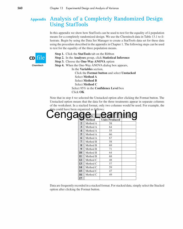
Appendix Analysis of a Completely Randomized DesignUsing StatToolsIn this appendix we show how StatTools can be used to test for the equality of k populationmeans for a completely randomized design. We use the Chemitech data in Table 13.1 to il-lustrate. Begin by using the Data Set Manager to create a StatTools data set for these datausing the procedure described in the appendix in Chapter 1. The following steps can be usedto test for the equality of the three population means.
Step 1. Click the StatTools tab on the RibbonStep 2. In the Analyses group, click Statistical InferenceStep 3. Choose the One-Way ANOVA optionStep 4. When the One-Way ANOVA dialog box appears,
In the Variables section,Click the Format button and select UnstackedSelect Method ASelect Method BSelect Method C
Select 95% in the Confidence Level boxClick OK
Note that in step 4 we selected the Unstacked option after clicking the Format button. TheUnstacked option means that the data for the three treatments appear in separate columnsof the worksheet. In a stacked format, only two columns would be used. For example, thedata could have been organized as follows:
560 Chapter 13 Experimental Design and Analysis of Variance
fileCDChemitech
Data are frequently recorded in a stacked format. For stacked data, simply select the Stackedoption after clicking the Format button.
A B C1 Method Units Produced2 Method A 583 Method A 644 Method A 555 Method A 666 Method A 677 Method B 588 Method B 699 Method B 71
10 Method B 6411 Method B 6812 Method C 4813 Method C 5714 Method C 5915 Method C 4716 Method C 4917
56130_13_ch13_p508-560.qxd 2/22/08 11:04 PM Page 560
Cengage Learning