Inference for a population mean

BPS chapter 18

© 2006 W. H. Freeman and Company

Objectives (BPS chapter 18)Inference about a Population Mean

Conditions for inference

The t distribution

The one-sample t confidence interval

Using technology

Matched pairs t procedures

Robustness of t procedures

Conditions for inference about a mean

We can regard our data as a simple random sample (SRS) from the

population. This condition is very important.

Observations from the population have a Normal distribution with mean

and standard deviation . In practice, it is enough that the distribution

be symmetric and single-peaked unless the sample is very small. Both

and standard deviation are unknown.

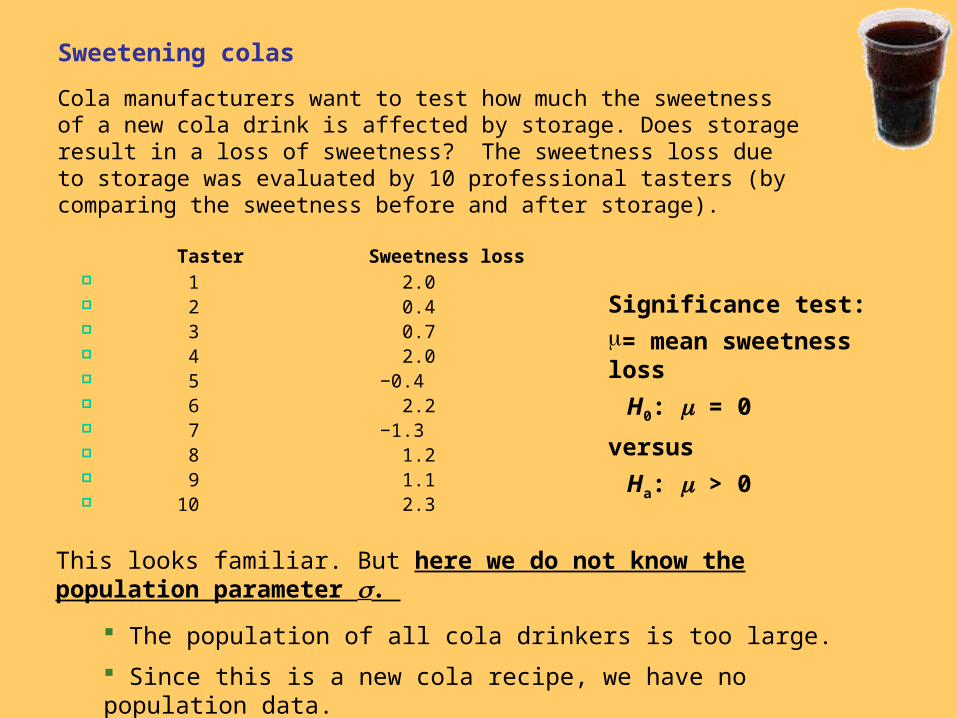
Sweetening colas

Cola manufacturers want to test how much the sweetness of a new cola drink is affected by storage. Does storage result in a loss of sweetness? The sweetness loss due to storage was evaluated by 10 professional tasters (by comparing the sweetness before and after storage).

Significance test:= mean sweetness loss

H0: = 0

versus

Ha: > 0

This looks familiar. But here we do not know the population parameter .

The population of all cola drinkers is too large.

Since this is a new cola recipe, we have no population data.

This situation is very common with real data.

Taster Sweetness loss 1 2.0 2 0.4 3 0.7 4 2.0 5 −0.4 6 2.2 7 −1.3 8 1.2 9 1.1 10 2.3

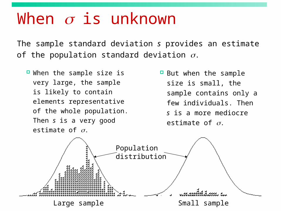
When is unknown

When the sample size is very

large, the sample is likely to

contain elements

representative of the whole

population. Then s is a very

good estimate of .

But when the sample size is

small, the sample contains

only a few individuals. Then s

is a more mediocre estimate

of .

The sample standard deviation s provides an estimate of the

population standard deviation .

Large sample Small sample

Populationdistribution

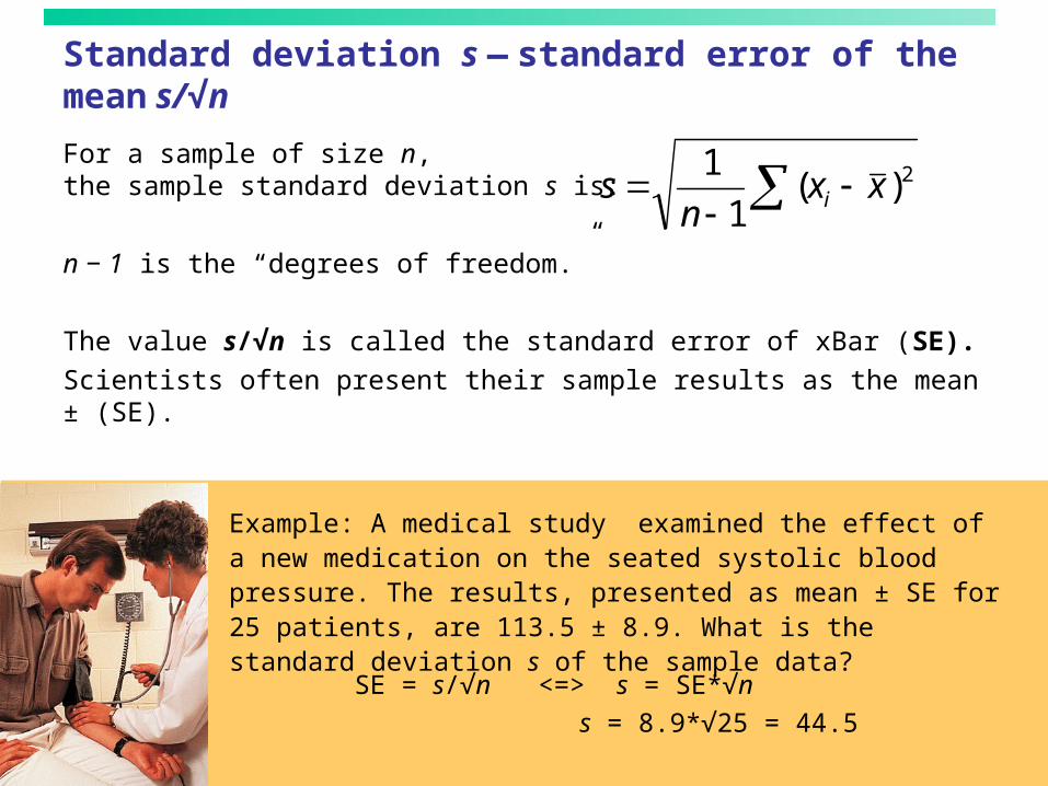
Example: A medical study examined the effect of a new medication on the seated systolic blood pressure. The results, presented as mean ± SE for 25 patients, are 113.5 ± 8.9. What is the standard deviation s of the sample data?

Standard deviation s — standard error of the mean s/√n

For a sample of size n,the sample standard deviation s is:

n − 1 is the “degrees of freedom.”

The value s/√n is called the standard error of xBar (SE).

Scientists often present their sample results as the mean ± (SE).

2)(1

1xx

ns i

SE = s/√n <=> s = SE*√n

s = 8.9*√25 = 44.5

The t distributions

We test a null and alternative hypotheses with one sample of size n from

a normal population N(µ,σ):

When is known, the sampling distribution is normal N(/√n).

When is estimated from the sample standard deviation s, then the

sampling distribution follows a t distribution t(,s/√n) with degrees of

freedom n − 1.

The value (s/√n) is the standard error of xBar (SE).

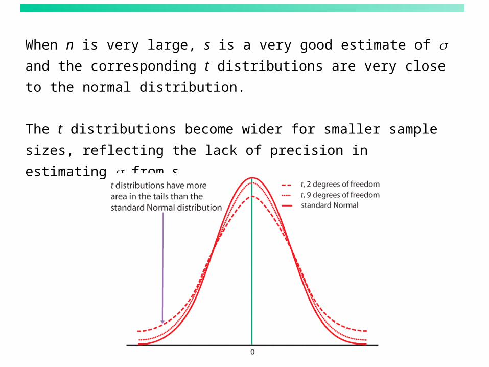
When n is very large, s is a very good estimate of and the

corresponding t distributions are very close to the normal distribution.

The t distributions become wider for smaller sample sizes, reflecting

the lack of precision in estimating from s.

Standardizing the data before using Table C

Here, is the mean (center) of the sampling distribution,

and the standard error of the mean s/√n is its standard deviation (width).

You obtain s, the standard deviation of the sample, with your calculator.

t

t x s n

As with the normal distribution, the first step is to standardize the data.

Then we can use a calculator or Table C to obtain the area under the

curve.

Sampling distribution of xBar

t()df = n − 1

x 0

1

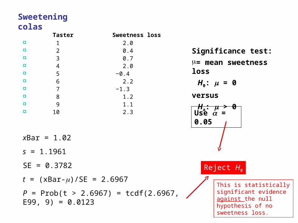
Sweetening colas

Significance test:= mean sweetness loss

H0: = 0

versus

Ha: > 0

Taster Sweetness loss 1 2.0 2 0.4 3 0.7 4 2.0 5 −0.4 6 2.2 7 −1.3 8 1.2 9 1.1 10 2.3

xBar = 1.02

s = 1.1961

SE = 0.3782

t = (xBar-)/SE = 2.6967

P = Prob(t > 2.6967) = tcdf(2.6967, E99, 9) = 0.0123

Use = 0.05

Reject H0

This is statistically significant evidence against the null hypothesis of no sweetness loss.

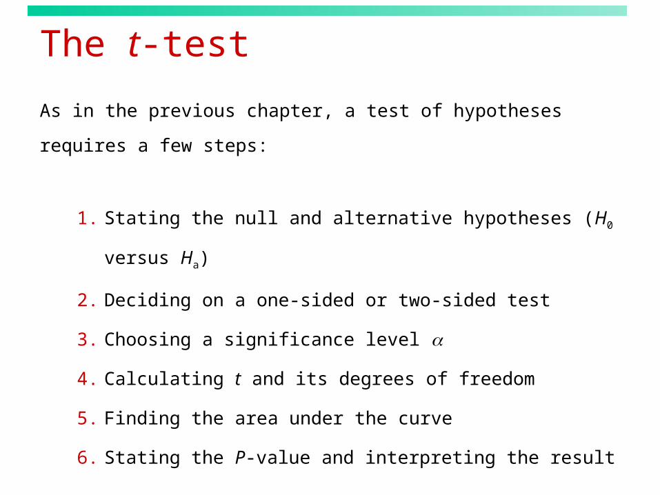
The t-test

As in the previous chapter, a test of hypotheses requires a few steps:

1. Stating the null and alternative hypotheses (H0 versus Ha)

2. Deciding on a one-sided or two-sided test

3. Choosing a significance level

4. Calculating t and its degrees of freedom

5. Finding the area under the curve

6. Stating the P-value and interpreting the result

t x s n

One-sided (one-tailed)

Two-sided (two-tailed)

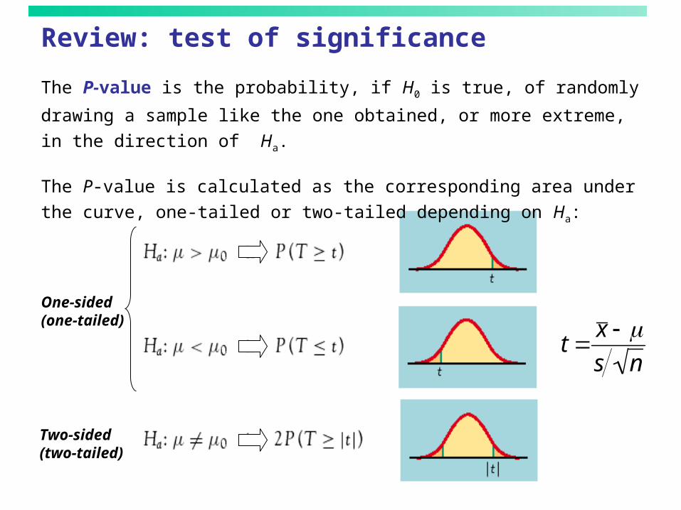
Review: test of significance

The P-value is the probability, if H0 is true, of randomly drawing a

sample like the one obtained, or more extreme, in the direction of Ha.

The P-value is calculated as the corresponding area under the curve,

one-tailed or two-tailed depending on Ha:

Confidence intervalsReminder: A confidence interval for is an interval that represents the

possible values for that are consistent with our random sample and our

chosen confidence level C. The confidence level C represents the

likelihood that a random sample will produce a confidence interval that

actually does contain the true mean .

C

t*−t*

m m

m t * s n

Practical use of t: t* C is the area under the t (df: n−1) curve between −t* and t*.We find t* using the TI-84 or Table C (for df = n−1 and confidence level C).The margin of error m is:

Red wine, in moderation

Drinking red wine in moderation may protect against heart attacks. The

polyphenols it contains act on blood cholesterol and thus are a likely cause.

To test the hypothesis that moderate red wine consumption increases the

average blood level of polyphenols, a group of nine randomly selected healthy

men were assigned to drink half a bottle of red wine daily for 2 weeks. Their

blood polyphenol levels were assessed before and after the study and the

percent change is presented here:

Firstly: Are the data approximately normal?

0.7 3.5 4 4.9 5.5 7 7.4 8.1 8.4

Normal?

When the sample size is small, histograms can be difficult to interpret.

Histogram

0

1

2

3

4

2.5 5 7.5 9 More

Percentage change in polyphenols blood levels

Fre

quen

cy

There is a low value, but overall the data can be considered reasonably normal.

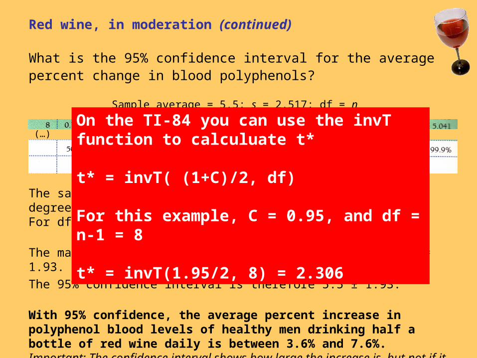
Red wine, in moderation (continued)

What is the 95% confidence interval for the average percent change in blood polyphenols?

Sample average = 5.5; s = 2.517; df = n − 1 = 8

(…)

The sampling distribution is a t distribution with n − 1 degrees of freedom. For df = 8 and C = 95%, t* = 2.306.

The margin of error m is : m = t*s/√n = 2.306*2.517/√9 ≈ 1.93.

The 95% confidence interval is therefore 5.5 ± 1.93.

With 95% confidence, the average percent increase in polyphenol blood levels of healthy men drinking half a bottle of red wine daily is between 3.6% and 7.6%. Important: The confidence interval shows how large the increase is, but not if it can have an impact on men’s health.

On the TI-84 you can use the invT function to calculuate t*

t* = invT( (1+C)/2, df)

For this example, C = 0.95, and df = n-1 = 8

t* = invT(1.95/2, 8) = 2.306

Matched pairs t proceduresSometimes we want to compare treatments or conditions at the

individual level. These situations produce two samples that are not

independent — they are related to each other. The members of one

sample are identical to, or matched (paired) with, the members of the

other sample.

Example: Pre-test and post-test studies look at data collected on the

same sample elements before and after some experiment is performed.

Example: Twin studies often try to sort out the influence of genetic

factors by comparing a variable between sets of twins.

Example: Using people matched for age, sex, and education in social

studies allows us to cancel out the effect of these potential lurking

variables.

In these cases, we use the paired data to test the difference in the two

population means. The variable studied becomes X = x1 − x2, and

H0: µdifference=0; Ha: µdifference>0 (or <0, or ≠0)

Conceptually, this does not differ from tests on one population.

Sweetening colas (revisited)

The sweetness loss due to storage was evaluated by 10 professional

tasters (comparing the sweetness before and after storage):

Taster Sweetness loss 1 2.0 2 0.4 3 0.7 4 2.0 5 −0.4 6 2.2 7 −1.3 8 1.2 9 1.1 10 2.3

We want to test if storage

results in a loss of

sweetness, thus

H0: = 0 versus Ha: > 0

Although the text did not mention it explicitly, this is a pre-/post-test design,

and the variable is the difference in cola sweetness before and after storage.

A matched pairs test of significance is indeed just like a one-sample test.

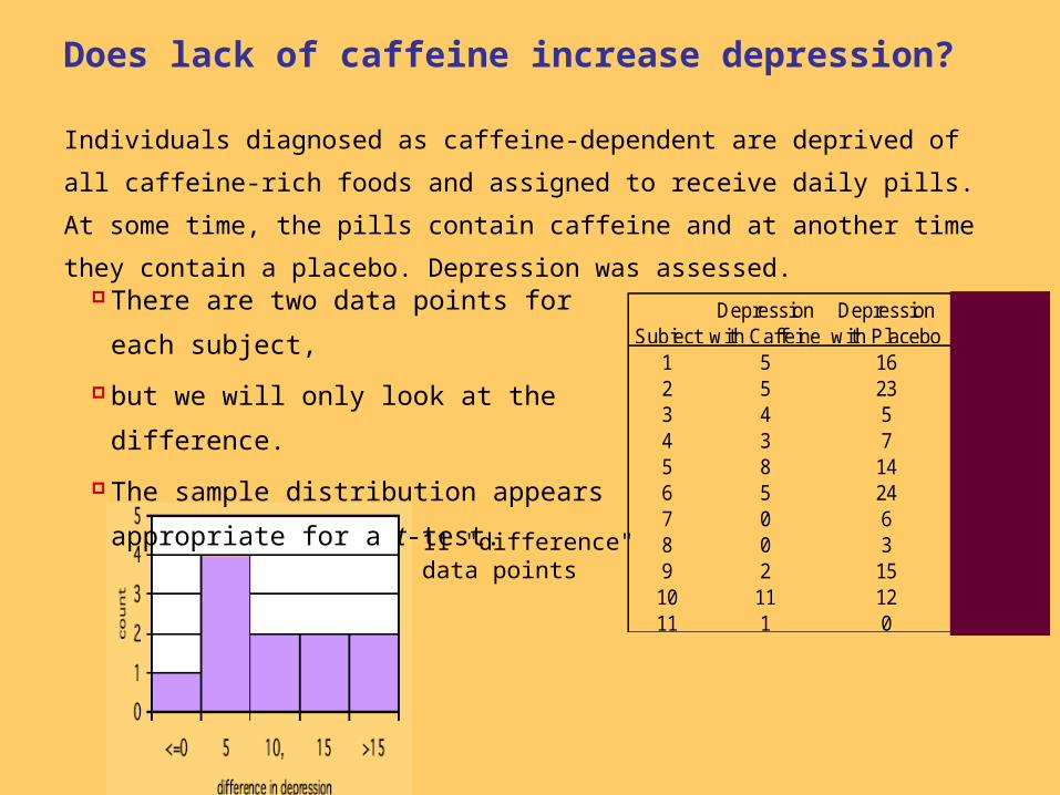
Does lack of caffeine increase depression?

Individuals diagnosed as caffeine-dependent are deprived of all caffeine-rich

foods and assigned to receive daily pills. At some time, the pills contain caffeine

and at another time they contain a placebo. Depression was assessed.

SubjectDepression

with CaffeineDepression

with PlaceboPlacebo - Cafeine

1 5 16 112 5 23 183 4 5 14 3 7 45 8 14 66 5 24 197 0 6 68 0 3 39 2 15 1310 11 12 111 1 0 -1

11 "difference" data points

There are two data points for each subject,

but we will only look at the difference.

The sample distribution appears

appropriate for a t-test.

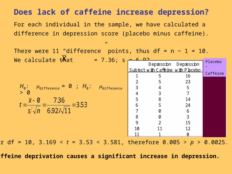
Does lack of caffeine increase depression?

For each individual in the sample, we have calculated a difference in depression

score (placebo minus caffeine).

There were 11 “difference” points, thus df = n − 1 = 10.

We calculate that = 7.36; s = 6.92

H0: difference = 0 ; H0: difference > 0

53.311/92.6

36.70

ns

xt

SubjectDepression

with CaffeineDepression

with PlaceboPlacebo - Cafeine

1 5 16 112 5 23 183 4 5 14 3 7 45 8 14 66 5 24 197 0 6 68 0 3 39 2 15 1310 11 12 111 1 0 -1

For df = 10, 3.169 < t = 3.53 < 3.581, therefore 0.005 > p > 0.0025.

Caffeine deprivation causes a significant increase in depression.

x Placebo -

Caffeine

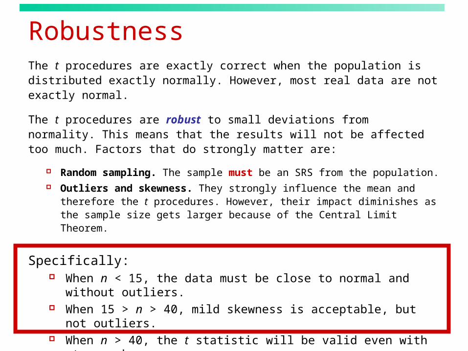
RobustnessThe t procedures are exactly correct when the population is distributed exactly normally. However, most real data are not exactly normal.

The t procedures are robust to small deviations from normality. This means that the results will not be affected too much. Factors that do strongly matter are:

Random sampling. The sample must be an SRS from the population. Outliers and skewness. They strongly influence the mean and

therefore the t procedures. However, their impact diminishes as the sample size gets larger because of the Central Limit Theorem.

Specifically: When n < 15, the data must be close to normal and without outliers. When 15 > n > 40, mild skewness is acceptable, but not outliers. When n > 40, the t statistic will be valid even with strong skewness.

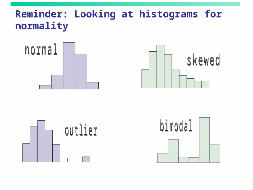
Reminder: Looking at histograms for normality