inf 2310 – digital bildebehandling• many problems cannot be solved using convolutional nets, so...

F1 21.08.18 IN 5520 1

IN55200 – Digital Image Analysis

Fritz Albregtsen & Anne H.S. Solberg 21.08.2018

IntroductIon

•Practical information

•What will you learn in this course? •Examples of applications of digital image analysis

•Repetition of key material from INF2310

F1 21.08.18 IN 5520 2

• Fritz Albregtsen – IFI/UiO (Fourth floor, room 4459, OJD building) – Telephone: 22852463 / 911 63 005 – Email: [email protected]

• Anne Schistad Solberg

– IFI/UiO (Fourth floor, room 4458, OJD building) – Telephone: 22852435 – Email: [email protected]

• Kristine – Email: [email protected]

Practical information - Lecturers

F1 21.08.18 IN 5520 3

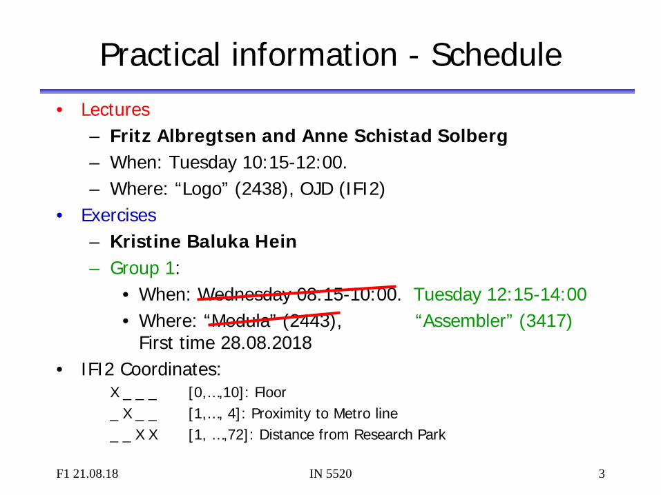
Practical information - Schedule • Lectures

– Fritz Albregtsen and Anne Schistad Solberg – When: Tuesday 10:15-12:00. – Where: “Logo” (2438), OJD (IFI2)

• Exercises – Kristine Baluka Hein – Group 1:

• When: Wednesday 08:15-10:00. Tuesday 12:15-14:00 • Where: “Modula” (2443), “Assembler” (3417)

First time 28.08.2018 • IFI2 Coordinates:

X _ _ _ [0,…,10]: Floor _ X _ _ [1,…, 4]: Proximity to Metro line _ _ X X [1, …,72]: Distance from Research Park

F1 21.08.18 IN 5520 4

Web page

• http://www.uio.no/studier/emner/matnat/ifi/IN5520/

– Information about the course – Lecture plan – Lecture notes – Exercise material – Course requisite description – Exam information – Messages

F1 21.08.18 IN 5520 5

Course material

• All slides will be made available on the course web site. • The slides define the course requisites. • Exercises will be introduced as we go along.

• No books defining all course requisites

– Gonzalez & Woods: Digital Image Processing, 3rd ed., 2008. + additional material

F1 21.08.18 IN 5520 6

Exercises

• The ordinary weekly exercises are NOT obligatory. – But definitely a good idea to do them anyway – The ordinary exercises can be solved in any programming

language, solutions will be provided in Matlab.

• Mandatory exercises (“term project”) – Two parts (October & November) – Individual work

– A little extra work for PhD-students taking this course as IN9520

F1 21.08.18 IN 5520 7

Exam

• Written exam ( 4 hours), date is not determined yet …

• No written sources of information allowed at exam

• A little extra work for PhD-students taking this course as IN9520

• Follow the web page for updates on the exam.

F1 21.08.18 IN 5520 8

Term project

• Sadly, we see plagiarism and cheating on term papers, but the reaction may be severe.

• Therefore you should read the following document: www.uio.no/studier/admin/obligatoriske-aktiviteter/mn-ifi-oblig.html (in Norwegian) Please notice routines on cheating and plagiarism!

• Using available source code and applications is perfectly

OK and will be credited as long as the origin is cited

• The term project is individual work, and the handed in result should clearly be your own work

F1 21.08.18 IN 5520 9

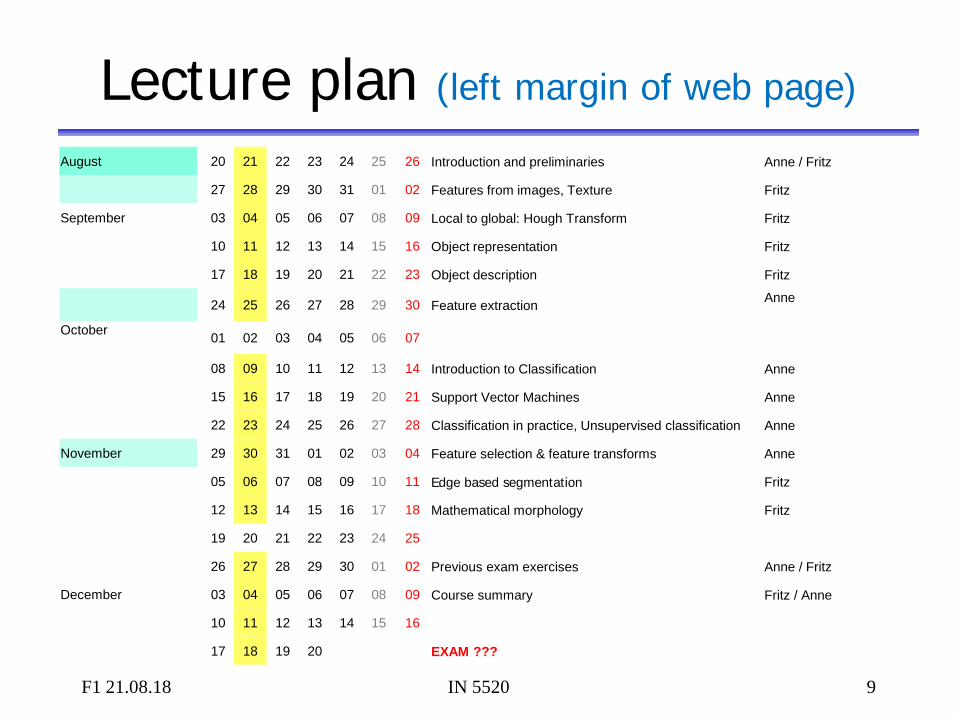
Lecture plan (left margin of web page)

August 20 21 22 23 24 25 26 Introduction and preliminaries Anne / Fritz

27 28 29 30 31 01 02 Features from images, Texture Fritz

September 03 04 05 06 07 08 09 Local to global: Hough Transform Fritz

10 11 12 13 14 15 16 Object representation Fritz

17 18 19 20 21 22 23 Object description Fritz

24 25 26 27 28 29 30 Feature extraction Anne

October 01 02 03 04 05 06 07

08 09 10 11 12 13 14 Introduction to Classification Anne

15 16 17 18 19 20 21 Support Vector Machines Anne

22 23 24 25 26 27 28 Classification in practice, Unsupervised classification Anne

November 29 30 31 01 02 03 04 Feature selection & feature transforms Anne

05 06 07 08 09 10 11 Edge based segmentation Fritz

12 13 14 15 16 17 18 Mathematical morphology Fritz

19 20 21 22 23 24 25

26 27 28 29 30 01 02 Previous exam exercises Anne / Fritz

December 03 04 05 06 07 08 09 Course summary Fritz / Anne

10 11 12 13 14 15 16

17 18 19 20 EXAM ???

F1 21.08.18 IN 5520 10

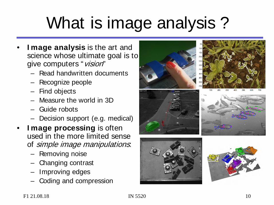
What is image analysis ? • Image analysis is the art and

science whose ultimate goal is to give computers “vision” – Read handwritten documents – Recognize people – Find objects – Measure the world in 3D – Guide robots – Decision support (e.g. medical)

• Image processing is often used in the more limited sense of simple image manipulations: – Removing noise – Changing contrast – Improving edges – Coding and compression

F1 21.08.18 IN 5520 11

From pixels to features to class

• Objects often correspond to regions. We need the spatial relationship between the pixels.

• For text recognition: the information is in the shape, not in the gray levels.

• Classification: learn features that are common for one type of objects.

Region features: •Area •Perimeter •Curvature •Moment of inertia •Topology •....

Region feature extraction

Segmentation Classification 3

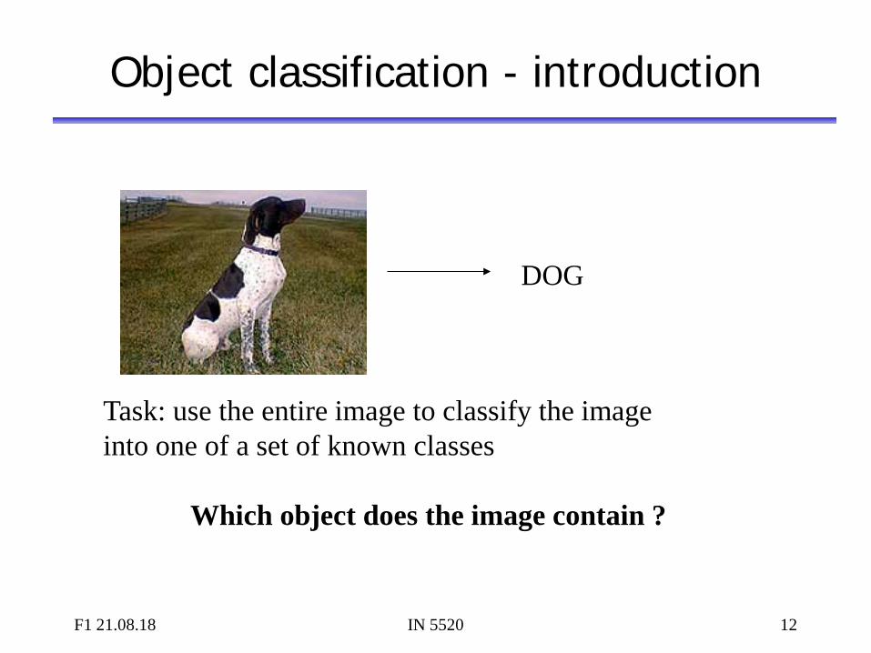
Object classification - introduction

F1 21.08.18 IN 5520 12

DOG

Task: use the entire image to classify the image into one of a set of known classes Which object does the image contain ?

IN 5520

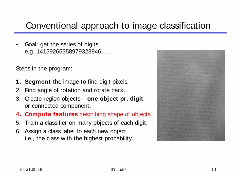
Conventional approach to image classification

• Goal: get the series of digits, e.g. 14159265358979323846……

Steps in the program:

1. Segment the image to find digit pixels. 2. Find angle of rotation and rotate back. 3. Create region objects – one object pr. digit

or connected component. 4. Compute features describing shape of objects 5. Train a classifier on many objects of each digit. 6. Assign a class label to each new object,

i.e., the class with the highest probability.

13 F1 21.08.18

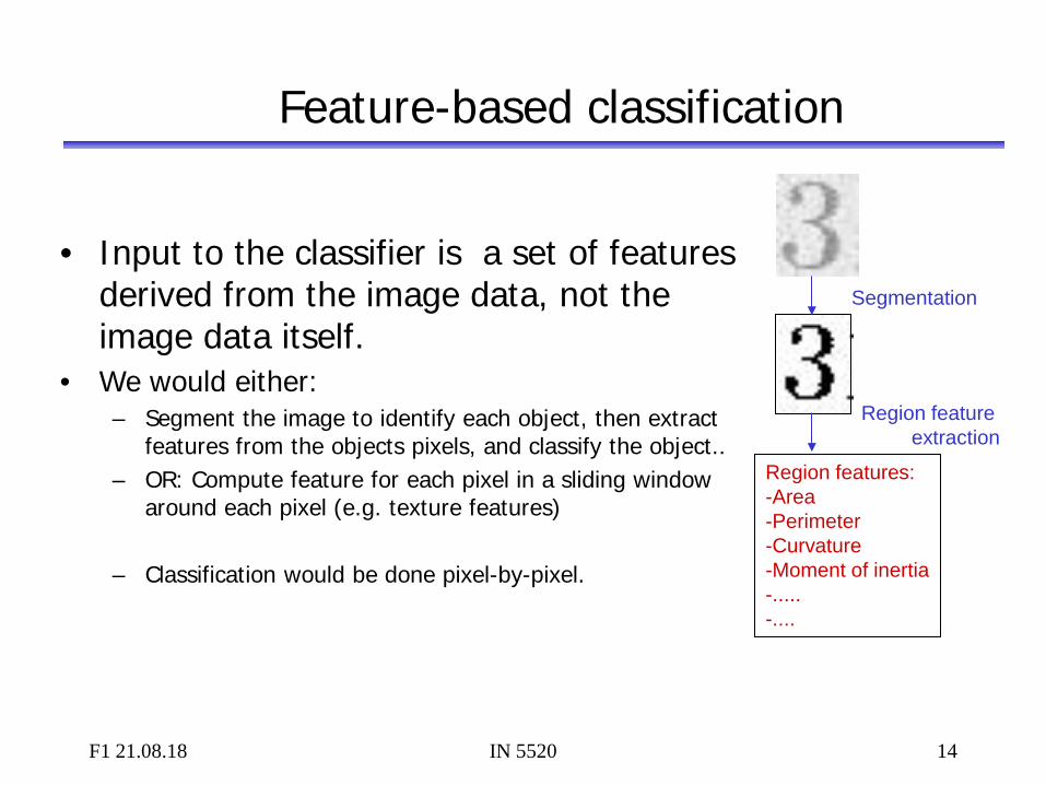
Feature-based classification

• Input to the classifier is a set of features

derived from the image data, not the image data itself.

• We would either: – Segment the image to identify each object, then extract

features from the objects pixels, and classify the object.. – OR: Compute feature for each pixel in a sliding window

around each pixel (e.g. texture features)

– Classification would be done pixel-by-pixel.

Region features: -Area -Perimeter -Curvature -Moment of inertia -..... -....

Region feature extraction

Segmentation

14 F1 21.08.18 IN 5520

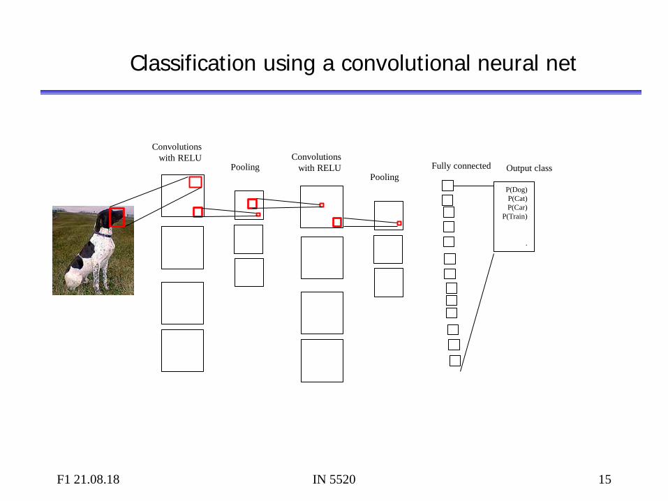
Classification using a convolutional neural net

F1 21.08.18 IN 5520 15

Convolutions with RELU

Pooling Convolutions

with RELU Pooling

Fully connected Output class

P(Dog) P(Cat) P(Car)

P(Train)

.

State-of-the art image classification

• Deep learning using convolutional nets (INF 5860)

can solve many image classification problems – In particular: classify ONE object in an image – Steady progress each year

• Many problems cannot be solved using convolutional nets,

so traditional image analysis methods are highly needed.

• A good basis for image analysis and machine learning is: – IN 55200 (Fall) – INF 5860 Machine learning for image analysis (Spring)

F1 21.08.18 IN 5520 16

F1 21.08.18 IN 5520 17

Applications of image analysis …

• Medical applications, e.g., ultrasound, MR, cell images • Industrial inspection • Traffic surveillance • Text recognition, document handling • Coding and compression • Biometry

– identification by face recognition, fingerprint or iris

• Earth resource mapping by satellite images • Sea-bed mapping (sonar) • Mapping of oil reservoirs (seismic)

F1 21.08.18 IN 5520 18

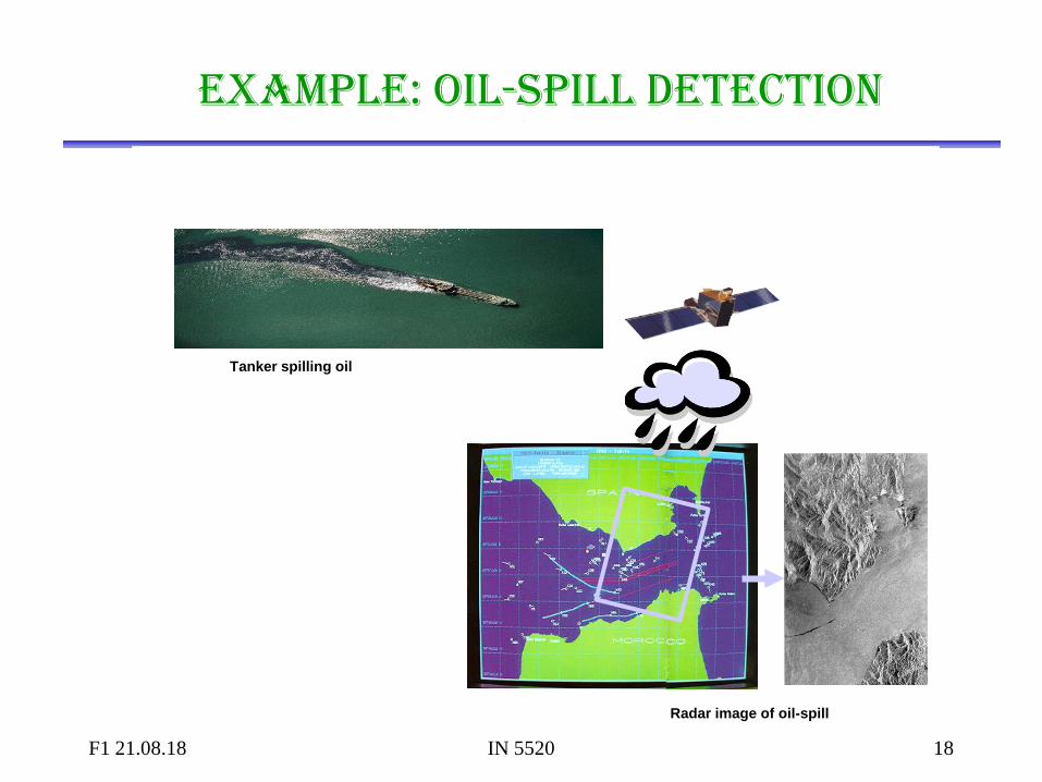
Deteksjon av oljesøl fra radarbilder

Tanker spilling oil

Radar image of oil-spill

ExamplE: oIl-spIll dEtEctIon

F1 21.08.18 IN 5520 19

ExamplE: tIssuE classIfIcatIon In mr ImagEs

MR images of brain

Classification into tissue

types. Tumor marked

in red.

F1 21.08.18 IN 5520 20

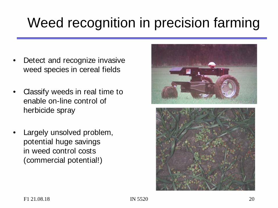
Weed recognition in precision farming

• Detect and recognize invasive weed species in cereal fields

• Classify weeds in real time to enable on-line control of herbicide spray

• Largely unsolved problem, potential huge savings in weed control costs (commercial potential!)

F1 21.08.18 IN 5520 21

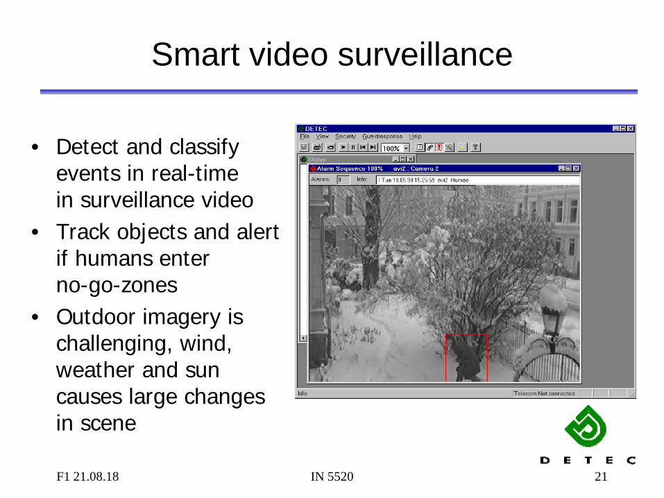
Smart video surveillance

• Detect and classify events in real-time in surveillance video

• Track objects and alert if humans enter no-go-zones

• Outdoor imagery is challenging, wind, weather and sun causes large changes in scene

F1 21.08.18 IN 5520 22

Tracking and classification of objects

Challenges: Objects may be poorly

segmented or occluded, so shape or appearance models may be useless

One blob may contain several objects

Solutions: Analyze motion patterns within

blobs (decide object class) Detect heads, arms and other

human parts (decide number of objects within blob)

F1 21.08.18 IN 5520 23

Automatic fish segmentation

• Pick single fish from underwater video of a fish farm

• Estimation of fish statistics – Size (for weight estimates) – Motion

• Challenges: – Illumination varies – Seawater murky, food / particles – No contrast – Fish overlap – Fish may swim in any direction

• Solution: – Active contours, initialized with a

fish-shape – Use information from two cameras

F1 21.08.18 IN 5520 24

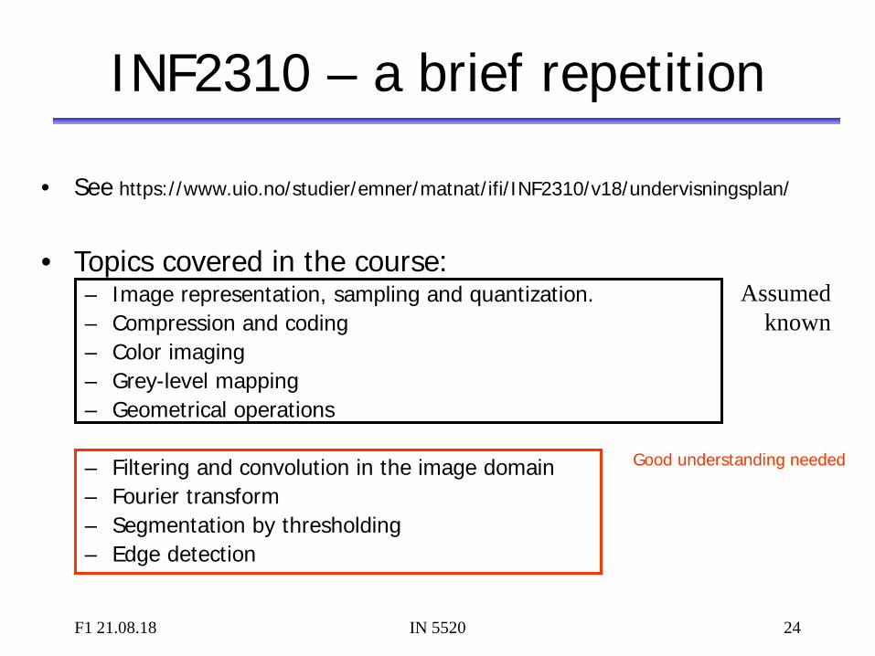
INF2310 – a brief repetition

• See https://www.uio.no/studier/emner/matnat/ifi/INF2310/v18/undervisningsplan/

• Topics covered in the course:

– Image representation, sampling and quantization. – Compression and coding – Color imaging – Grey-level mapping – Geometrical operations

– Filtering and convolution in the image domain – Fourier transform – Segmentation by thresholding – Edge detection

Assumed known

Good understanding needed

F1 21.08.18 IN 5520 25

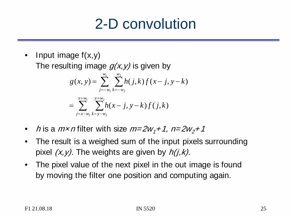
2-D convolution

• Input image f(x,y) The resulting image g(x,y) is given by

• h is a m×n filter with size m=2w1+1, n=2w2+1 • The result is a weighed sum of the input pixels surrounding

pixel (x,y). The weights are given by h(j,k). • The pixel value of the next pixel in the out image is found

by moving the filter one position and computing again.

∑ ∑

∑ ∑+

−=

+

−=

−= −=

−−=

−−=

1

1

2

2

1

1

2

2

),(),(

),(),(),(

wx

wxj

wy

wyk

w

wj

w

wk

kjfkyjxh

kyjxfkjhyxg

F1 21.08.18 IN 5520 26

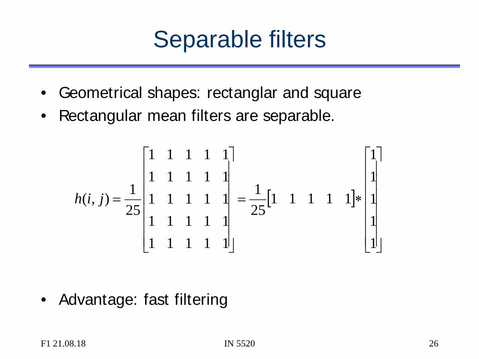
Separable filters

• Geometrical shapes: rectanglar and square • Rectangular mean filters are separable.

• Advantage: fast filtering

[ ]

∗=

=

11111

11111251

1111111111111111111111111

251),( jih

F1 21.08.18 IN 5520 27

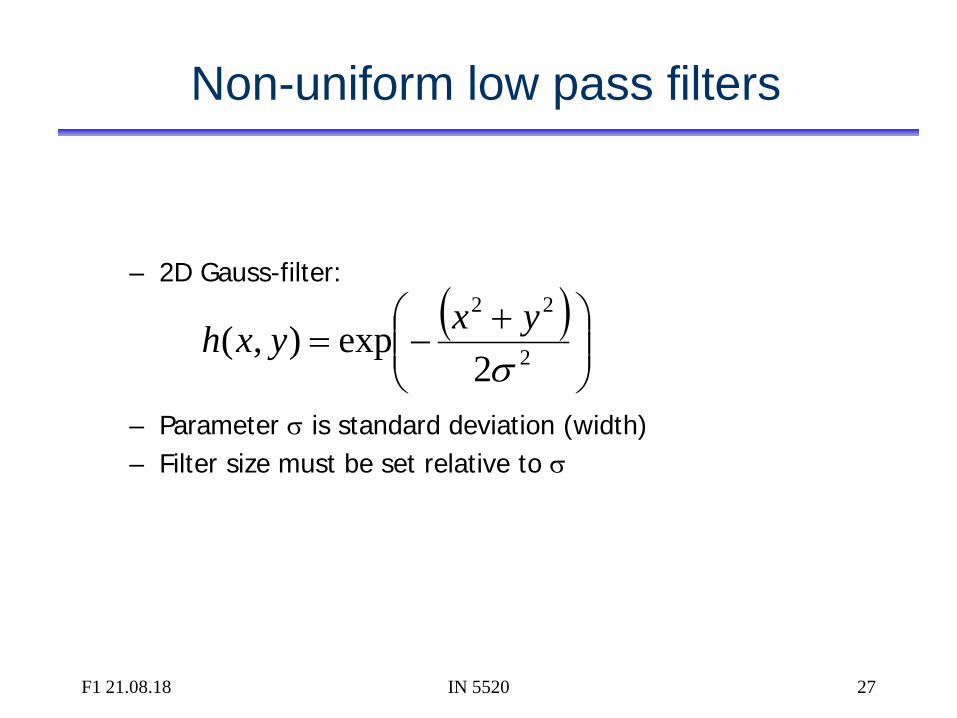
Non-uniform low pass filters

– 2D Gauss-filter:

– Parameter σ is standard deviation (width) – Filter size must be set relative to σ

( )

+−= 2

22

2exp),(

σyxyxh

F1 21.08.18 IN 5520 28

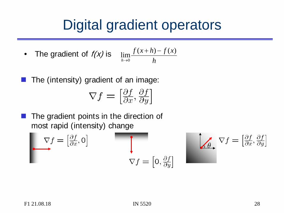
Digital gradient operators • The gradient of f(x) is

hxfhxf

h

)()(lim0

−+→

The (intensity) gradient of an image:

The gradient points in the direction of

most rapid (intensity) change

F1 21.08.18 IN 5520 29

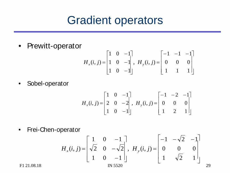
Gradient operators

• Prewitt-operator

• Sobel-operator

• Frei-Chen-operator

−−−=

−−−

=111000111

),(,101101101

),( jiHjiH yx

−−−=

−−−

=121000121

),(,101202101

),( jiHjiH yx

−−−=

−−−

=121000121

),(,101202

101),( jiHjiH yx

F1 21.08.18 IN 5520 30

Gradient direction and magnitude

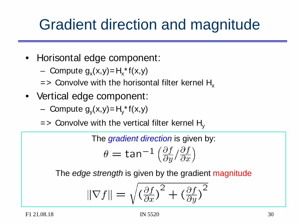
• Horisontal edge component: – Compute gx(x,y)=Hx*f(x,y) => Convolve with the horisontal filter kernel Hx

• Vertical edge component: – Compute gy(x,y)=Hy*f(x,y)

=> Convolve with the vertical filter kernel Hy

The gradient direction is given by:

The edge strength is given by the gradient magnitude

F1 21.08.18 IN 5520 31

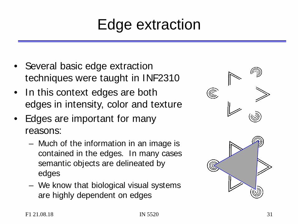
Edge extraction

• Several basic edge extraction techniques were taught in INF2310

• In this context edges are both edges in intensity, color and texture

• Edges are important for many reasons: – Much of the information in an image is

contained in the edges. In many cases semantic objects are delineated by edges

– We know that biological visual systems are highly dependent on edges

F1 21.08.18 IN 5520 32

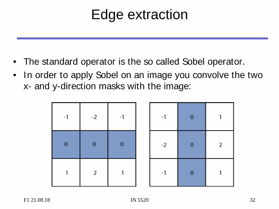
Edge extraction

• The standard operator is the so called Sobel operator. • In order to apply Sobel on an image you convolve the two

x- and y-direction masks with the image:

F1 21.08.18 IN 5520 33

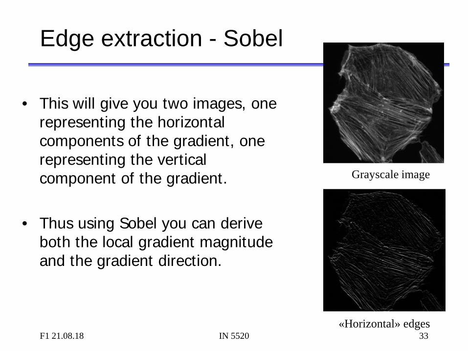
Edge extraction - Sobel

• This will give you two images, one representing the horizontal components of the gradient, one representing the vertical component of the gradient.

• Thus using Sobel you can derive both the local gradient magnitude and the gradient direction.

Grayscale image

«Horizontal» edges

F1 21.08.18 IN 5520 34

Edge extraction - Laplace

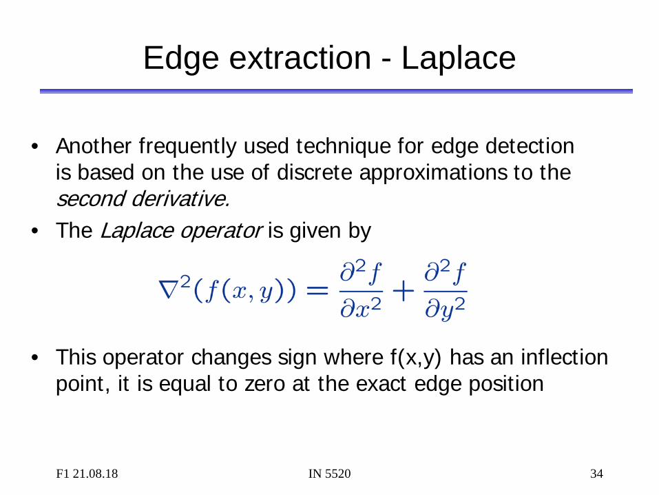
• Another frequently used technique for edge detection is based on the use of discrete approximations to the second derivative.

• The Laplace operator is given by

• This operator changes sign where f(x,y) has an inflection point, it is equal to zero at the exact edge position

F1 21.08.18 IN 5520 35

Edge extraction - Laplace

• Approximating second derivatives on images as finite differences gives the following mask

F1 21.08.18 IN 5520 36

Edge extraction - LoG

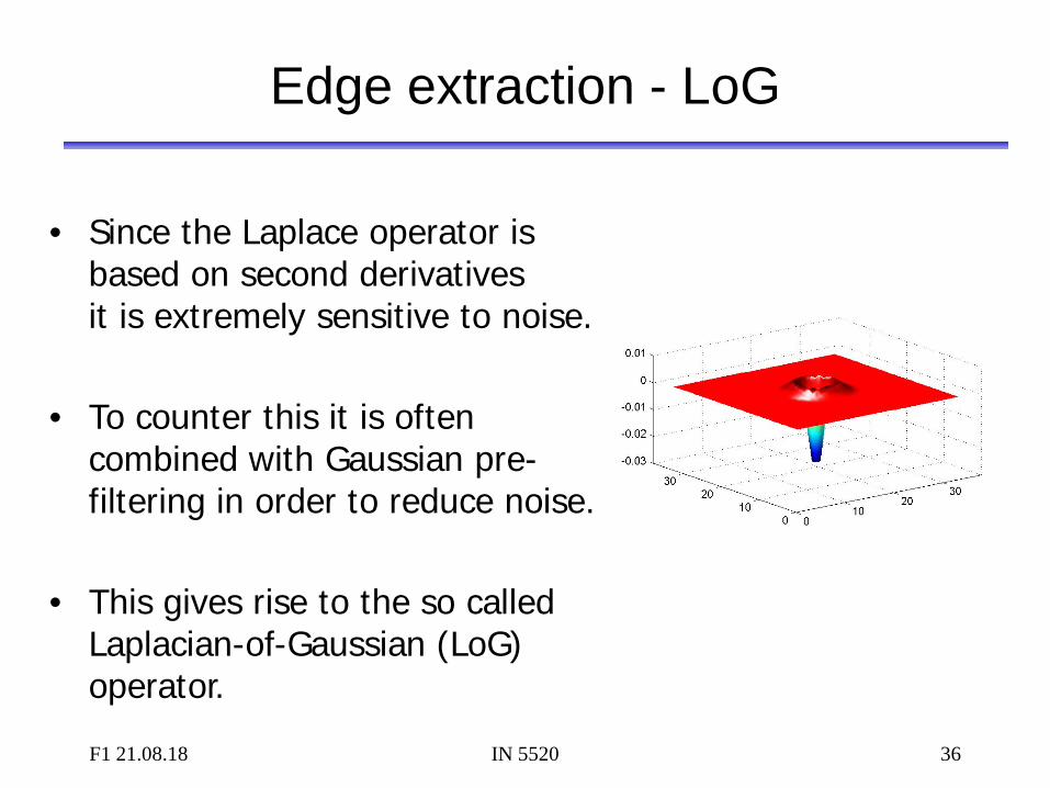
• Since the Laplace operator is based on second derivatives it is extremely sensitive to noise.

• To counter this it is often combined with Gaussian pre-filtering in order to reduce noise.

• This gives rise to the so called Laplacian-of-Gaussian (LoG) operator.

F1 21.08.18 IN 5520 37

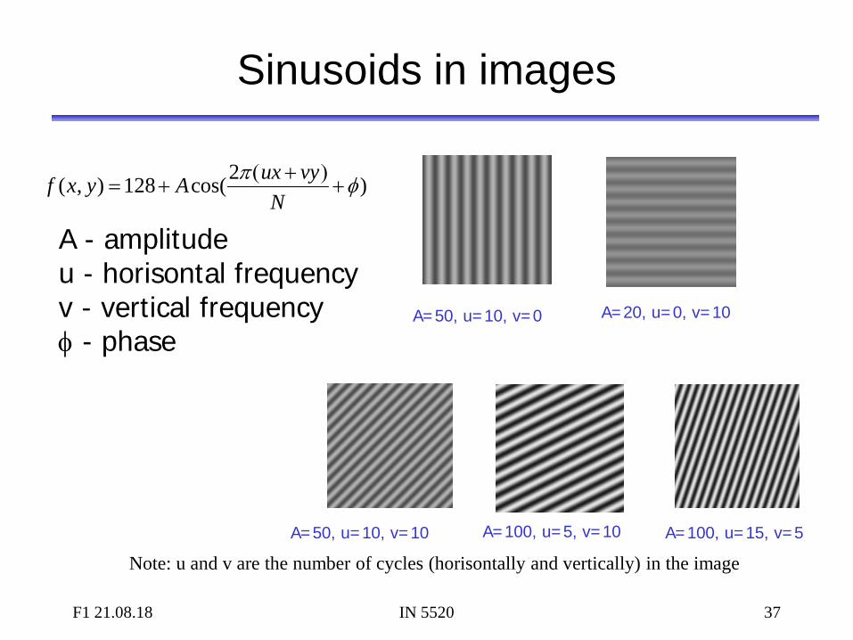
Sinusoids in images

A - amplitude u - horisontal frequency v - vertical frequency φ - phase

)2cos(128),( φπ+

)+(+=

NvyuxAyxf

A=50, u=10, v=0 A=20, u=0, v=10

A=100, u=15, v=5 A=100, u=5, v=10 A=50, u=10, v=10

Note: u and v are the number of cycles (horisontally and vertically) in the image

F1 21.08.18 IN 5520 38

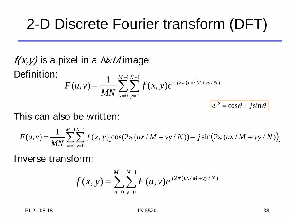
2-D Discrete Fourier transform (DFT)

f(x,y) is a pixel in a N×M image Definition: This can also be written: Inverse transform:

∑∑−

=

−

=

+−=1

0

1

0

)//(2),(1),(M

x

N

y

NvyMuxjeyxfMN

vuF π

( )[ ]∑∑−

=

−

=

+−+=1

0

1

0)//(2sin))//(2cos(),(1),(

M

x

N

yNvyMuxjNvyMuxyxf

MNvuF ππ

∑∑−

=

−

=

+=1

0

1

0

)//(2),(),(M

u

N

v

NvyMuxjevuFyxf π

θθθ sincos je j +=

F1 21.08.18 IN 5520 39

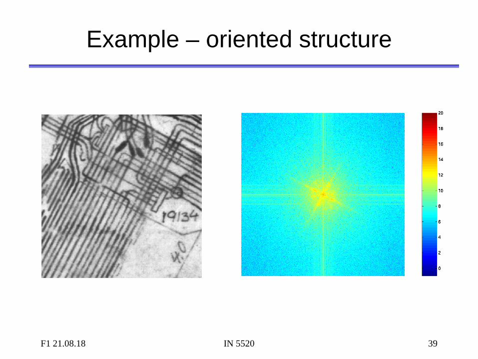
Example – oriented structure

F1 21.08.18 IN 5520 40

The convolution theorem

Convolution in the image domain ⇔

Multiplication in the frequency domain

Multiplication in the image domain ⇔

Convolution in the frequency domain

),(),(),(),( vuHvuFyxhyxf ⋅⇔∗

),(),(),(),( vuHvuFyxhyxf ∗⇔⋅

F1 21.08.18 IN 5520 41

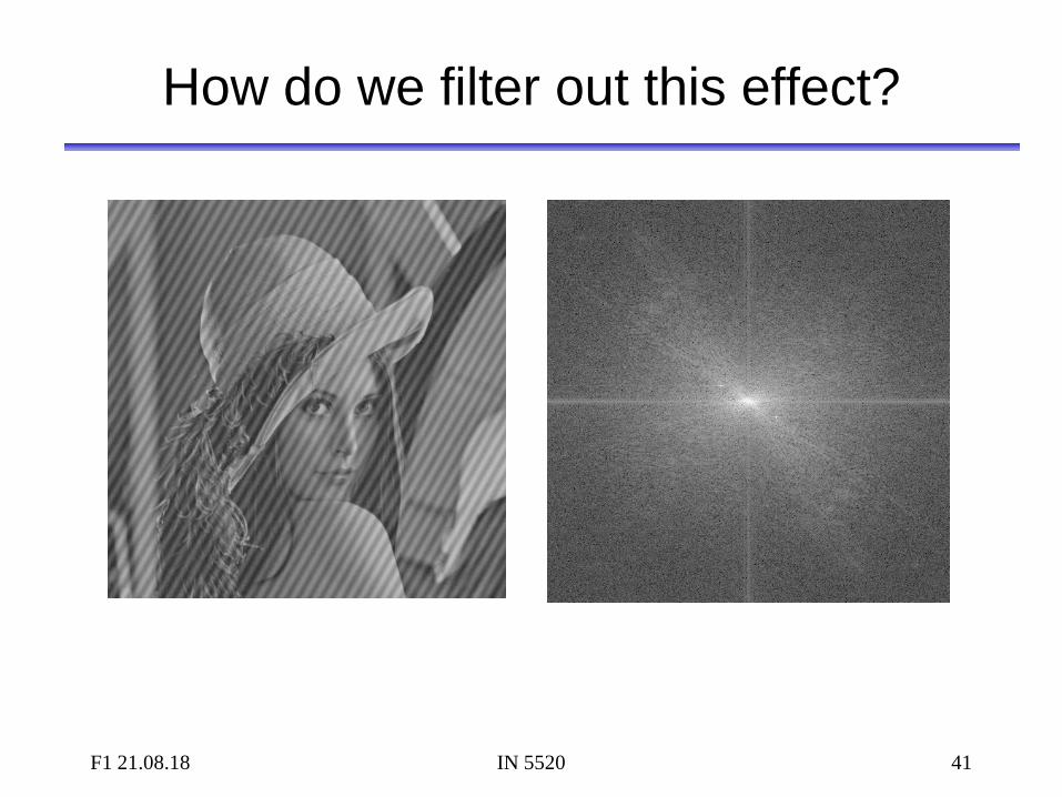
How do we filter out this effect?

F1 21.08.18 IN 5520 42

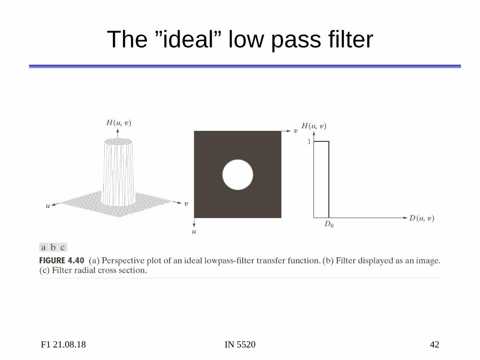
The ”ideal” low pass filter

F1 21.08.18 IN 5520 43

Example - ideal low pass

Original D0=0.2 D0=0.3

Look at these image in high resolution. You should see ringing effects in the two rightmost images.

F1 21.08.18 IN 5520 44

What causes the ringing effect?

• Note that the filter profile has negative coefficients

• It has similar profile to a Mexican-hat filter (Laplace-of-Gaussian)

• The radius of the circle and the number of circles per unit is inversely proportional to the cutoff frequency – Low cutoff gives large radius

in image domain

fft of H(u,v) for ideal lowpass

1D profile for ideal lowpass

Ideal lowpass in the image domain

F1 21.08.18 IN 5520 45

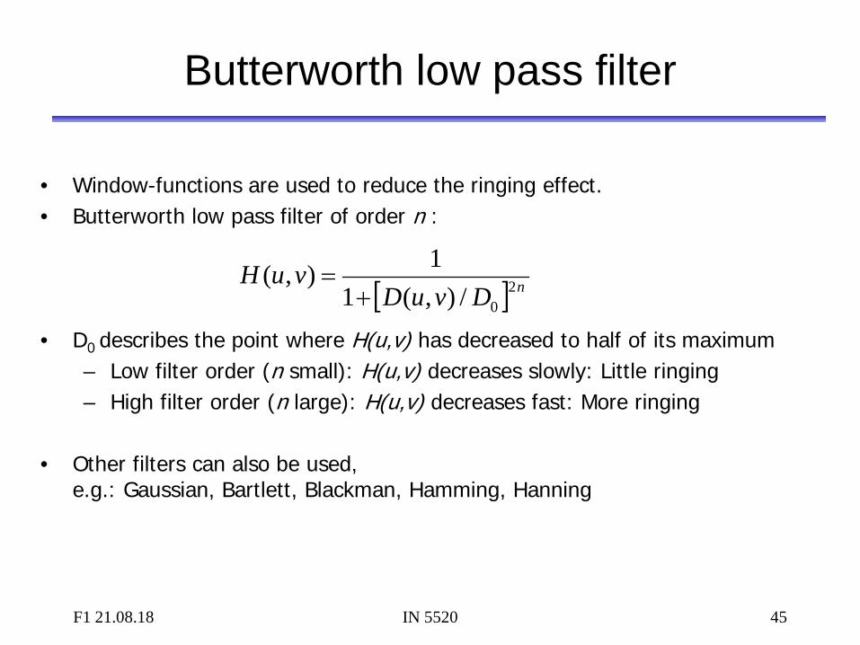
Butterworth low pass filter

• Window-functions are used to reduce the ringing effect. • Butterworth low pass filter of order n :

• D0 describes the point where H(u,v) has decreased to half of its maximum – Low filter order (n small): H(u,v) decreases slowly: Little ringing – High filter order (n large): H(u,v) decreases fast: More ringing

• Other filters can also be used,

e.g.: Gaussian, Bartlett, Blackman, Hamming, Hanning

[ ] nDvuDvuH 2

0/),(11),(

+=

F1 21.08.18 IN 5520 46

Gaussian lowpass filter

22 2/),(),( σvuDevuH −=

F1 21.08.18 IN 5520 47

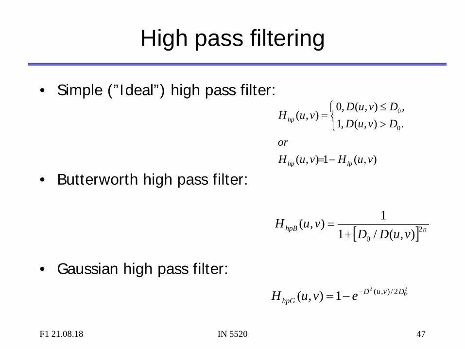
High pass filtering

• Simple (”Ideal”) high pass filter:

• Butterworth high pass filter:

• Gaussian high pass filter:

),(1),(

.),(,1,),(,0

),(0

0

vuHvuHor

DvuDDvuD

vuH

lphp

hp

−=

>≤

=

[ ] nhpB vuDDvuH 2

0 ),(/11),(

+=

20

2 2/),(1),( DvuDhpG evuH −−=

F1 21.08.18 IN 5520 48

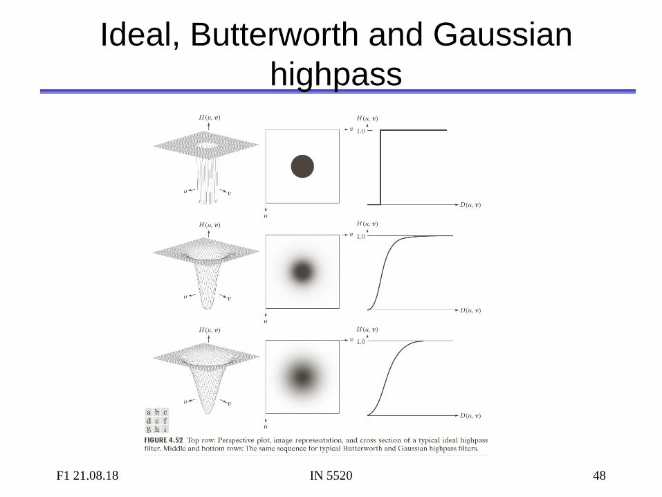
Ideal, Butterworth and Gaussian highpass

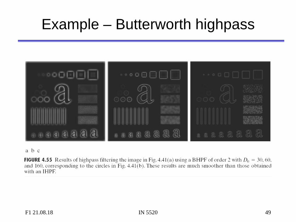
F1 21.08.18 IN 5520 49

Example – Butterworth highpass

F1 21.08.18 IN 5520 50

Bandpass and bandstop filters

• Bandpass filter: Keeps only the energy in a given frequency band <Dlow,Dhigh> (or <D0-W/2,D0+ W/2>)

• W is the width of the band • D0 is its radial center.

• Bandstop filter: Removes all energy in a given frequency band <Dlow,Dhigh>

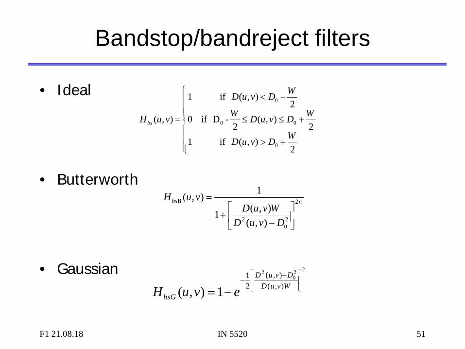
F1 21.08.18 IN 5520 51

Bandstop/bandreject filters

• Ideal

• Butterworth

• Gaussian

+>

+≤≤

−<

=

2),( if1

2),(

2-D if0

2),( if1

),(

0

00

0

WDvuD

WDvuDW

WDvuD

vuHbs

nbs

DvuDWvuD

vuH 2

20

2 ),(),(1

1),(

−

+

=B

220

2

),(),(

21

1),(

−−

−= WvuDDvuD

bsG evuH

F1 21.08.18 IN 5520 52

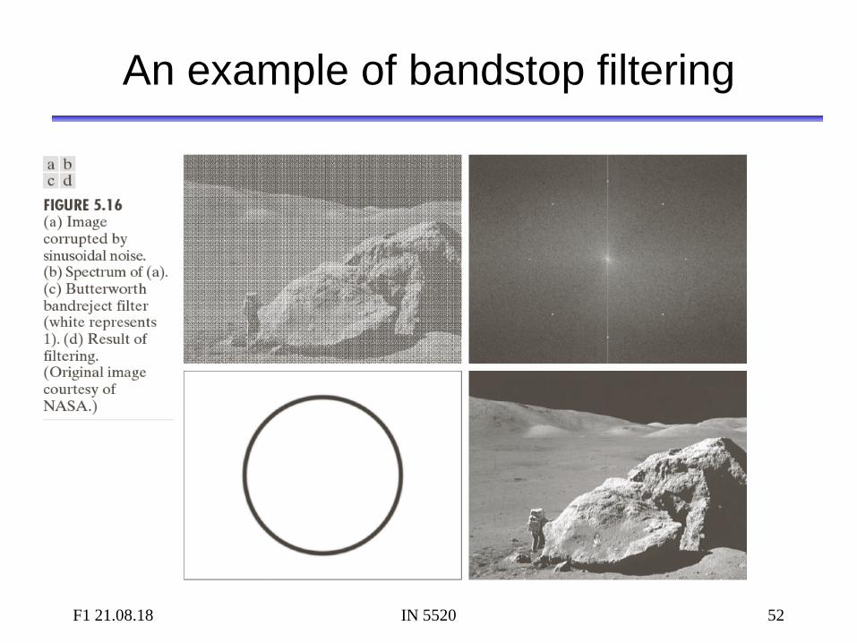
An example of bandstop filtering

F1 21.08.18 IN 5520 53

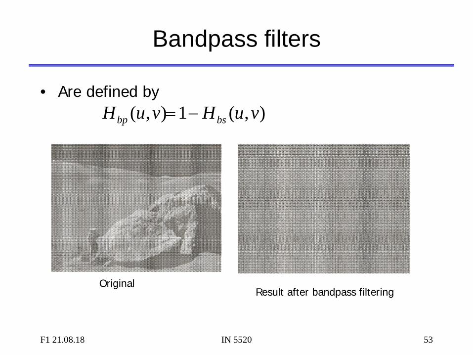
Bandpass filters

• Are defined by ),(1),( vuHvuH bsbp −=

Original Result after bandpass filtering

F1 21.08.18 IN 5520 54

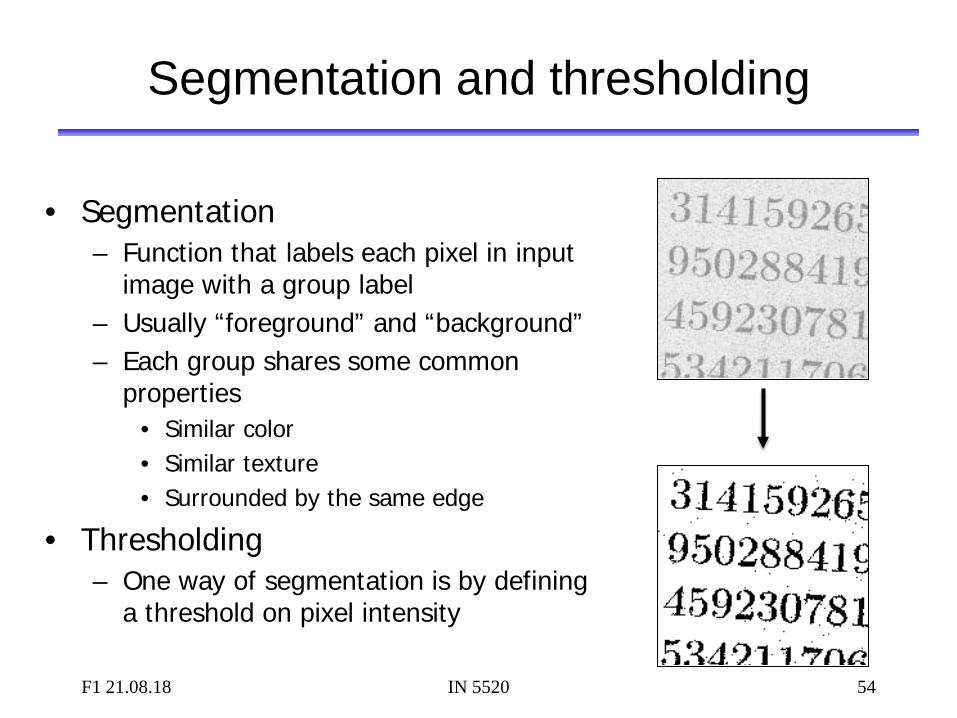
Segmentation and thresholding

• Segmentation – Function that labels each pixel in input

image with a group label – Usually “foreground” and “background” – Each group shares some common

properties • Similar color • Similar texture • Surrounded by the same edge

• Thresholding – One way of segmentation is by defining

a threshold on pixel intensity

F1 21.08.18 IN 5520 55


Remember, regions that have semantic importance do not always have any particular local visual distinction.

F1 21.08.18 IN 5520 56


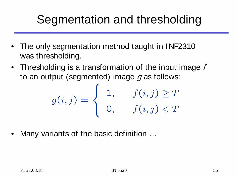
• The only segmentation method taught in INF2310 was thresholding.

• Thresholding is a transformation of the input image f to an output (segmented) image g as follows:

• Many variants of the basic definition …

F1 21.08.18 IN 5520 57


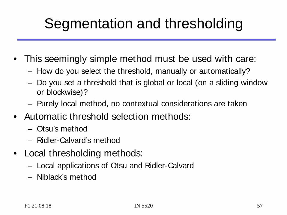
• This seemingly simple method must be used with care: – How do you select the threshold, manually or automatically? – Do you set a threshold that is global or local (on a sliding window

or blockwise)? – Purely local method, no contextual considerations are taken

• Automatic threshold selection methods: – Otsu’s method – Ridler-Calvard’s method

• Local thresholding methods: – Local applications of Otsu and Ridler-Calvard – Niblack’s method

F1 21.08.18 IN 5520 58


• Remember that you normally make an error performing a segmentation using thresholding:

F1 21.08.18 IN 5520 59


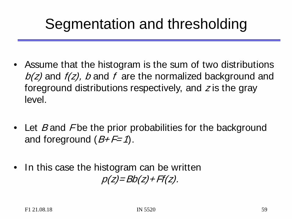
• Assume that the histogram is the sum of two distributions b(z) and f(z), b and f are the normalized background and foreground distributions respectively, and z is the gray level.

• Let B and F be the prior probabilities for the background and foreground (B+F=1).

• In this case the histogram can be written p(z)=Bb(z)+Ff(z).

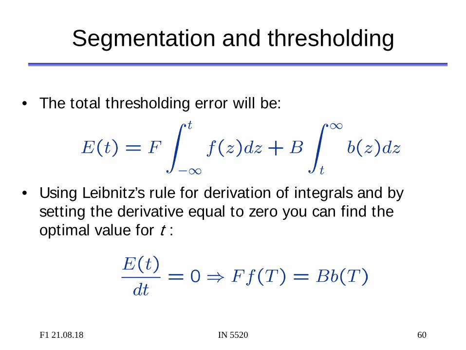
F1 21.08.18 IN 5520 60


• The total thresholding error will be:

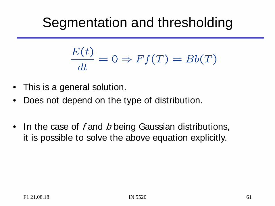
• Using Leibnitz’s rule for derivation of integrals and by setting the derivative equal to zero you can find the optimal value for t :

F1 21.08.18 IN 5520 61


• This is a general solution. • Does not depend on the type of distribution.

• In the case of f and b being Gaussian distributions,

it is possible to solve the above equation explicitly.

F1 21.08.18 IN 5520 62


• In INF2310 we introduced two methods

(Ridler-Calvard and Otsu) for determining segmentation thresholds automatically.

• Region- and edge-based methods will be covered in detail in the INF5520 lectures.

F1 21.08.18 IN 5520 63

Exercise & next lecture

• Exercise: Practical use of Matlab, see web page.

• Next lecture: Features from images – Texture analysis.

inf 2310 – digital bildebehandling• many problems cannot be solved using convolutional nets, so...

Documents