comparing convolutional neural networking and image

Comparing convolutional neural networking and image processing seismic fault

detection methods

Jie Qi, Bin Lyu, Xinming Wu, and Kurt Marfurt

[email protected], [email protected], [email protected], and [email protected]

Running Head: Deep learning application to seismic fault detection

Corresponding author:

Jie Qi

The University of Oklahoma, ConocoPhillips School of Geology and Geophysics

810E Sarkeys Energy Center

100 East Boyd Street

Norman, OK 73019

Abstract

Convolutional Neural Networks (CNN)-based fault detection is an emerging

technology that shows great promise for the seismic interpreter. One of the more successful

deep learning CNN methods uses synthetic data to train a CNN model. Although training

a CNN model is time-consuming, the CNN prediction and classification is extremely fast.

In this paper, we build a CNN architecture to predict faults from 3D seismic data. We begin

by building a U-net shape architecture CNN model, and then train this model with 250 3D

synthetic 128×128×128 voxel seismic amplitudesubvolumes where each voxel is labeled

as being a fault or not a fault. The training data exhibit different data quality, spectral

bandwidth, noise level, and structural complexity. After training, we apply the CNN to

detect faults on four different data volumes, each of which exhibits different noise levels

and geologic features. We compare the CNN results to a more conventional attribute-based

image processing fault enhancement and skeletonization workflow. When the faults cut the

stratigraphic reflectors close to perpendicular resulting in minimal stair step artifacts, the

traditional attribute-based approach provides higher resolution images than CNN. However,

when faults cut the reflectors at larger angles, the CNN-based approach provides more

continuous and less noisy fault images. Although not trained on listric faults, the CNN-

based approach provides promising results for listric faults where the attribute-based

approach totally fails. However, with the limited training data provided in this paper, the

CNN -based approach cannot map the sole of listric faults that are easily picked by a human

interpreter.

Introduction

Picking horizons and faults are key products of any seismic interpretation project.

Faults may cause a reservoir to seal or leak, Faults may indicate a wider, fractured fault

zone. Faults may provide a path for hydrocarbon migration and are critical to accurate

section restoration to map the evolution of the geologic structure through time. While good

horizon autopickers have been used for over thirty years, autopicking of faults has been

more problematic.

Traditional fault detection method is a time-consuming exercise based on hand-

picking a suite of fault sticks on a coarse grid of seismic lines, followed by passing a surface

between the sticks to form a fault surface. Seismic edge-detection attributes such as eigen-

structure coherence (Gersztenkorn and Marfurt, 1999), gradient structure tensor (Bakker,

2002), energy-ratio similarity (Chopra and Marfurt, 2007), variance (Van Bemmel and

Pepper, 200), automated fault extraction (Dorn et al., 2012), fault likelihood (Hale, 2013),

have been widely used to highlight faults on 3D seismic data for over two decades. Edge-

detection attributes can describe discontinuity surfaces, which can guide interpreters to

create fault patches using commercial interpretation tools. With the help of seismic

attributes computed on every line, the accuracy of seismic fault detection can be increased

and the time of fault picking accelerated.

Unfortunately, stratigraphic edges and seismic noise also give rise to discontinuities

in 3D seismic data, such that interpreters still need to spend time to differentiate fault from

other incoherent anomalies. Image processing filters and algorithms provide a partial

solution to this problem. Randen et al. (2001) and Pedersen et al. (2002) applied a swarm

intelligence algorithm. Cohen et al. (2006) proposed a local fault extraction that is based

on vertical and lateral directional filtering and thresholds. Barnes (2006) computed the

eigenvectors of a second-moment tensors then processed faults by dilation and expansion

on an edge-detection attribute. Wu and Hale (2016) proposed an automatic intersecting

fault interpretation technique based on directional voxel interpolation by fault likelihood,

dip, and strike. Dewett and Henza (2016) combined multiple spectrally limited coherence

images using a self-organizing map algorithm to enhance fault anomalies. Wu and Fomel

(2018) enhanced a fault detection attribute and generated fault surfaces using an optimal

surface voting method. Qi et al. (2017) improved on Barnes’ (2006) approach by applying

a Laplacian of a Gaussian filter, then skeletonized fault anomalies along fault surfaces. Qi

et al. (2018) further improved this workflow by preconditioning the data and attributes to

enhance and skeletonize faults.

Convolutional neural networks (CNN) is a rapidly evolving technology that has

applications that range from the recognition of faces for airport security to guiding

decisions made by self-driving cars. The typical use of fully-connected CNN methods for

computer visual recognition tasks requires large amounts of training data. As a supervised

deep learning algorithm, CNN contains feature extraction (convolution), feature learning,

parameter updating, and feature localizing steps (Figure 1). The size of a fully-connected

network can range from 8 to 10 layers, which result in millions of parameters. The use of

CNN in biomedical image processing (Ronneberger et al., 2015) is also one of the

important tasks in applications of deep learning methods. In applications of seismic

exploration, CNNs have been successfully applied to seismic stratigraphy interpretation

(Di et al., 2019; Wu and Zhang, 2019; Geng et al., 2019), seismic inversion (Das et al.,

2018; Biswas et al., 2019; Wang et al., 2019), salt interpretation (Shi et al., 2017;

Waldeland et al., 2018; Ye et al., 2019), first-break picking (Yuan et al., 2018), and seismic

facies analysis (Dramsch et al., 2018; Zhao, 2018). Among thrse, the CNN application to

fault detection has provided some of the more promising results. Over the past three years,

Huang et al. (2017), Guo et al. (2018), Zhao and Mukhopadhyay (2018), Xiong et al. (2018),

Li et al. (2019), Zhao (2019), and Wu et al. (2018, 2019) have shown that CNN can be

trained to detect faults, differentiating them from other non-fault discontinuities in the

seismic data.

In fault classification we have two classes: voxels that are a fault and voxels that

are not a fault. Using 3D blocks of seismic amplitude data that are 128 inlines by 128

crosslines by 128 samples in size, each of the 2,097,144 voxels in the block is assigned a

value of 1 (a fault) or 0 (not a fault) defining the labeled information needed for training.

Generating the training data using either carefully constructed synthetics or by manually

picking 3D data volumes is perhaps the most time-consuming component of CNN

classification. The actual training is also time consuming, although this process is computer

intensive rather than human interpreter intensive. Once trained, the actual application of

the CNN to a large 3D volume is quite fast – with the necessary convolutions being carried

out on a graphic processing unit with 4608 CUDA cores.

In this paper, we build a deep learning convolutional neural network trained on

synthetic training data and apply it to predict faults from three different data volumes. The

first dataset was acquired from offshore New Zealand and contains many vertical normal

faults. The second dataset is onshore data and was acquired in the Fort Worth Basin. The

third data set is from onshore Gulf of Mexico and exhibits listric faults. We analyze the

same data set using a more traditional seismic attribute/fault enhancement/skeletonization

workflow described by Qi et al. (2017 and 2018). We then compare the two results and

draw preliminary conclusions.

The CNN-based fault detection workflow

Training data preparing and augmentation

There are several tasks required in CNN image classification and segmentation.

First, we need to train the network using a suite of small 3D volumes that are “labeled”

voxel by voxel as to whether or not there is a faulting. The direct way to construct such

training data is to have an interpreter manually pick faults on a seismic amplitude volume.

The subsequent learning (such as a stochastic or mini-batch gradient descent) algorithm

then evaluates and updates the internal CNN model parameters. However, using real

seismic data to generate training data requires enormous amounts of data to work well,

with each block requiring the manual interpretation of 128 lines of seismic amplitude data.

An alternative method is to generate the training data by creating faulted synthetic

seismic amplitude volumes. An advantage of using synthetic data is that we can easily

define the size and the total number of training data pairs. In this paper, the dimension of

our 250 3D subvolumes measure 128×128×128. In each seismic data volume, parameters

of fault dip magnitude, dip azimuth, displacement, and the number of faults (between 1 and

8) are randomly chosen. The reflectors and stratigraphic variations are also randomly

generated by adding vertical planar shifts and lateral folds. The seismic spectrum and

bandwidth are additionally considered to vary across different training subvolumes. We

randomly generate reflector thickness and set the peak frequency of Ricker wavelet

between 30 Hz to 50 Hz. We add Gaussian noise to the synthetic seismic amplitude

data.wherethe standard deviation of Gaussian noise is randomly defined. to fall between 0

and 200% of the RMS amplitude of the reflectors. Representative training blocks are shown

in Figure 2. The first training sample exhibits very high signal-to-noise ratio with limited

lateral folding whereas the second training sample is noisy and its reflectors are strongly

folded. Note the steeply dipping faults in the second synthetic seismic model are difficult

to visually identify.

U-Net shape architecture CNN model

We build a modified U-Net architecture CNN model based on that proposed by

Ronneberger et al. (2015). We modify the number of filters and layers to evaluate the

performance of a pre-trained model applications to various faults in different real datasets.

Figure 3 show our U-Net architecture. We add nine blocks to extract features where each

block contains two filter layers followed by a max pooling operator. The input is fed into

a concatenation of different convolutional filters that are then fed into a decoder that

localizes the feature. Since we want to evaluate a trained model for different data fault

classification problems, the first convolution layer is with 32 3D filters, and the last

combination at the bottom of the U has 512 3D filters. The final network consists of 18

convolutional 3×3×3 filter layers with a stride of 1×1×1. Following each convolution filter

layer, we apply a Rectified Linear Unit (ReLU) as the activation function.

Unlike the typical autoencoder architecture that compresses data linearly, the U-

Net architecture performs deconvolution, such that the output size of the U-Net architecture

is equal to the input size. For this reason, we pad the output of each convolution to be the

same size as the input. The maximum pooling sizes are 2×2×2. In the expansive part, the

mathematically transposed convolutional operator are applied to perform upsampling of

the feature maps using the learnable parameters. Our model only outputs one channel

feature and uses a sigmoid activation function in the last layer.

U-Net model training

We feed the generated 250 synthetic amplitude volume and label pairs to the U-Net

shape architecture model for training. From these 250 pairs we randomly select 30 pairs

that are used to validate the training. The batch size of model training is 2, which means 2

training datasets go through through the mini-batch gradient descent learning algorithm

before updating the model parameters. Before training, we augment the data augmentation

through rotation, thereby increasing the number of models to 1000. Each model is rotated

by 90 degrees about the x, y, and z axes to create additional 3 volumes. The entire training

data is trained 50 times (resulting in 50 epochs). The learning rate is 0.0001, and the Adam

optimizer is implemented. We choose binary cross entropy to be the loss function:

𝐿(𝑦, �̂�) = −1

𝑁∑ (𝑦 ∗ log(�̂�) + (1 − 𝑦) ∗ log(1 − �̂�𝑖))𝑁𝑖=0 , (1)

where 𝑦 is the label, and �̂� is the predicted value, where our goal is minimize the distance

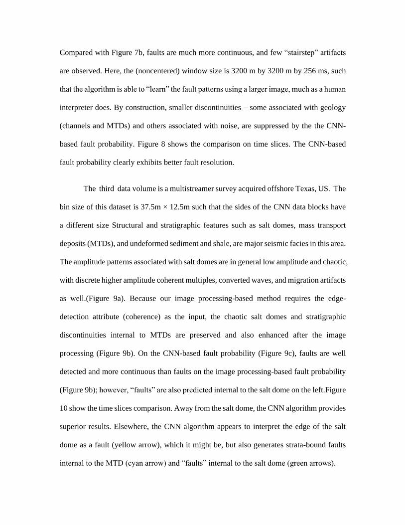
between the training and prediction labels. Figure 4 shows model accuracy and model loss.

Note the accuracy of the training is above 95%, and the validation loss is below 0.01.

Image processing-based fault detection workflow

For image processing-based fault detection method we use the fault enhancement

and skeletonization method described by Qi et al. (2017), Qi et al. (2018), and Lyu et al.

(2019).

. We begin with simple data conditioning that includes spectral balancing and

structure-oriented filtering which increases the bandwidth, improves the signal-to-noise

ratio, sharpens discontinuities, and suppress random and incoherent noise. The conditioned

data serve as input to multispectral coherence (Marfurt, 2017; Li et al. 2018). . For a poorly

defined fault, the coherence anomalies can be thought of as a cloud of values that can be

described by a center of mass, μ, and a 2nd moment tensor, I.. The mean value is defined

as :

𝜇𝑖 =∑ 𝑊𝑚𝑎𝑚𝑥𝑖𝑚𝑀𝑚=1

∑ 𝑊𝑚𝑀𝑚=1 𝑎𝑚

. (2)

where 𝑥𝑚the vector distance of the mth voxel from the center of the analysis window, 𝑎𝑚

is coherence anomalies within the analysis window and Wm is a measure of confidence in

our measure which we construct frp, the energy about each voxel. The second moment

tensor is

𝐼𝑗𝑘 = ∑ 𝑊𝑚(𝑥𝑗𝑚 − 𝜇𝑗)(𝑥𝑘𝑚 − 𝜇𝑘)𝑎𝑚𝑀𝑚=1 , (2)

To apply a directional Laplacian of Gaussian filter to fault anomalies in coherence, we

decompose the energy-weighted moment tensor to three eigenvectors 𝐯𝐣 . Taking into

account the hypothesized fault orientation (the eigenvectors 𝐯𝟏, 𝐯𝟐, and 𝐯𝟑), the Laplacian

of a Gaussian operator can directionally smooth parallel to fault surfaces and sharpen

perpendicular to fault surfaces. We iteratively apply the Laplacian of a Gaussian operator

until fault image is sufficiently smoothed and sharped. Finally, we skeletonize faults along

the perpendicular direction defined by the eigenvectors 𝐯𝟑.

Field data applications

We validate the CNN-based method and the image-processing based method to

three datasets. The first dataset is acquired from offshore New Zealand. We apply both

CNN-based and image processing-based fault detection methods to compute fault

probability. Figure 5 shows the comparison on vertical slices. Figure 5b shows the vertical

slice through seismic amplitude data co-rendered with the proposed CNN-based fault

probability, while Figure 5c shows seismic amplitude co-rendered with the image

processing-based fault enhancement and skeletonization fault probability. The image

processing-based fault probability exhibits good fault resolution. Note faults penetrating

the middle chaotic mass transport deposits are also detected. Figure 5c shows the fault

probability computed from the CNN U-Net architecture. Although the CNN fault

probability image exhibits less incoherent noise but also other non-fault related

discontinuities than the image processing-based fault probability image. More fault

anomalies can be observed in the CNN-based fault probability results. The image

processing-based fault probability is after skeletonization, thus the faults in Figure 5b

appear sharper than the faults in Figure 5c. Figure 6 shows time slice comparison. Note

faults in both fault probability results are continuous. The residual footprint anomalies

(blue arrow) can be observed on the image-processing based fault probability, but do not

exist on the CNN-based result.

Our second dataset is a early 3D single streamer marine data volume acquired on

the Louisiana Shelf, US. These data are contaminated by acquisition footprint and the

signal-to-noise ratio is low. The spectrum ranges between 10 Hz and 70 Hz. The major

faults in this dataset are high angle dipping faults, which cut each other and penetrate from

shallow to deep layers (Figure 7a). Figure 7b shows the vertical slice through seismic

amplitude co-rendered with the image processing-based fault probability. Fault anomalies

of Figure 7b exhibit strong “stairstep” artifacts (Lin and Marfurt, 20xx), which arise when

the orientation of the seismic wavelet (always perpendicular to the reflector) is not aligned

with the orientation of the fault. The size of the coherence computation was 50 m by 50 m

by 20 ms. The size of the LoG filter was 150 m by 150 m by 50 ms, such that the algorithms

do not “see” the larger fault pattern. Figure 7c shows the CNN-based fault probability.

Compared with Figure 7b, faults are much more continuous, and few “stairstep” artifacts

are observed. Here, the (noncentered) window size is 3200 m by 3200 m by 256 ms, such

that the algorithm is able to “learn” the fault patterns using a larger image, much as a human

interpreter does. By construction, smaller discontinuities – some associated with geology

(channels and MTDs) and others associated with noise, are suppressed by the the CNN-

based fault probability. Figure 8 shows the comparison on time slices. The CNN-based

fault probability clearly exhibits better fault resolution.

The third data volume is a multistreamer survey acquired offshore Texas, US. The

bin size of this dataset is 37.5m × 12.5m such that the sides of the CNN data blocks have

a different size Structural and stratigraphic features such as salt domes, mass transport

deposits (MTDs), and undeformed sediment and shale, are major seismic facies in this area.

The amplitude patterns associated with salt domes are in general low amplitude and chaotic,

with discrete higher amplitude coherent multiples, converted waves, and migration artifacts

as well.(Figure 9a). Because our image processing-based method requires the edge-

detection attribute (coherence) as the input, the chaotic salt domes and stratigraphic

discontinuities internal to MTDs are preserved and also enhanced after the image

processing (Figure 9b). On the CNN-based fault probability (Figure 9c), faults are well

detected and more continuous than faults on the image processing-based fault probability

(Figure 9b); however, “faults” are also predicted internal to the salt dome on the left.Figure

10 show the time slices comparison. Away from the salt dome, the CNN algorithm provides

superior results. Elsewhere, the CNN algorithm appears to interpret the edge of the salt

dome as a fault (yellow arrow), which it might be, but also generates strata-bound faults

internal to the MTD (cyan arrow) and “faults” internal to the salt dome (green arrows).

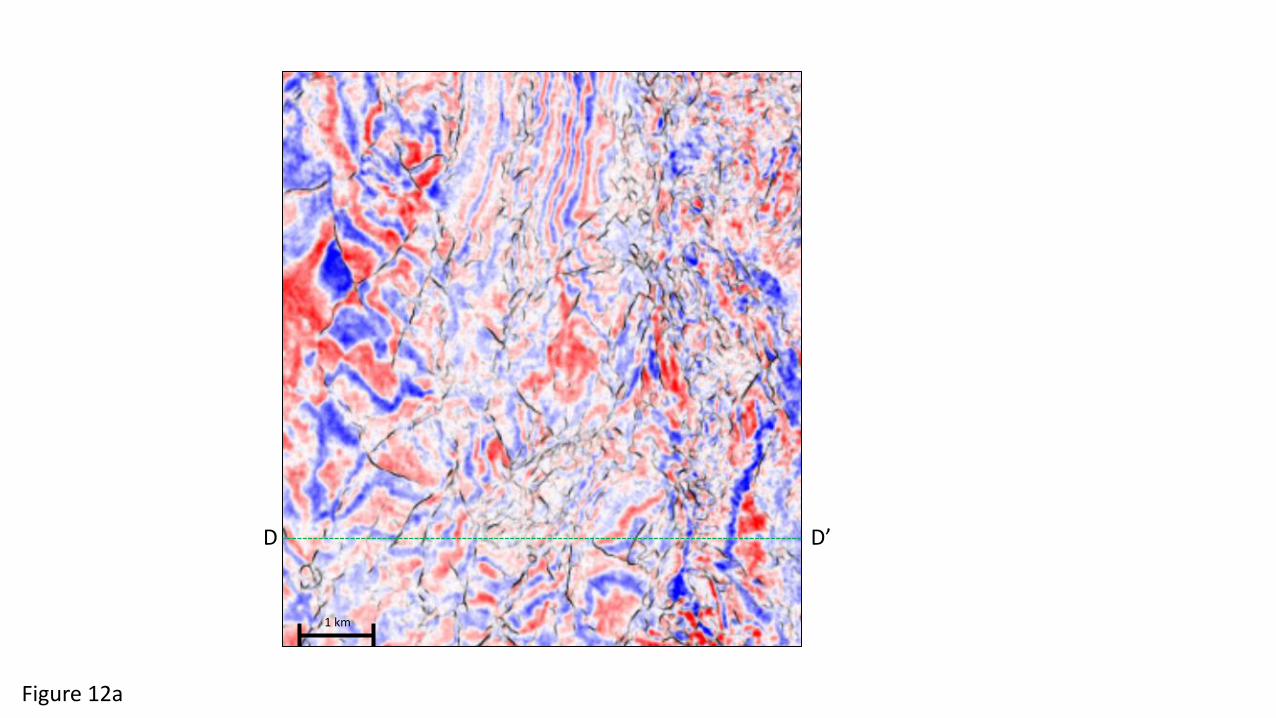
The fourth data volume comes from onshore south Texas, US, and exhibits high

angle listric faults that sole out into the deeper section.. This dataset is contaminated by

migration artifacts and random noise resulting in a lower signal-to-noise ratio, especially

in the deep area. Figure 11a show the vertical slices through the seismic amplitude volume.

We first compute the image processing-based fault probability (Figure 11b). Here, the

abundance of stairstep artifacts make the coherence image almost useless below t=1.8 s.

Figure 11c show the CNN fault probability, where the fault images are surprisingly good.

There are some obvious artifacts where the algorithm predicted faults subparallel to the

sedimentary reflectors (yellow arrows). The algorithm also does not continue the listric

fault on the right to region where it starts to sole out. Although CNN still shows non-fault

planar discontinuities, more of these artifacts are rejected compared with the image

processing fault probability.

We also compare the proposed CNN architecture with a simplified CNN

architecture. We simplify our proposed CNN architecture by decreasing layer and filter

number, which is similar to the one introduced by Wu et al. (2019). We train the new

simplified CNN model with the same training data and hyperparameters. The simplified

CNN result is shown in Figure 11d. Note that, the proposed complicated CNN workflow

shows slightly more continuous faults (indicated by green arrows in Figure 11c) and less

artifacts (indicated by orange arrows). Figure 12 compares time slices at t=1.52 s through

the CNN-based fault probability volumes comparing with image processing result. The

CNN result exhibits much better fault anomalies than the image processing-based result.

Discussions

We have compared the CNN method on fault detection with a more traditional fault

analysis workflows based on seismic attributes and image processing. Although the

synthetics we created to train the CNN mode are all normal faults, a common CNN practice

is to augment the training data by rotating and flipping each image. Different types of noise

are added to the synthetics to allow the algorithm to learn to see through the noise as a

human interpreter does. We add 9 blocks and a large number of filters into the CNN

architecture to extract fault features for fault detection on different dataset. The model is

well-trained after 50 epochs, and no over-training existed. In contrast to CNN, the image

processing “convolutions” have been predetermined based on geologic insight and

concepts of signal analysis. The image processing workflow includes noise suppression,

edge-detection attribute computation, image filter application, and image skeletonization.

In the first field data test, the data quality is good, and frequencies range between 5 and 80

Hz. The main challenge of fault detection in this dataset is to map faults penetrating through

mass transport deposits. The second example compares the capacity of these methods on

fault detection in the presence of strong seismic noise. This dataset is contaminated by

strong footprint (in the shallow area), and incoherent noise. When we created our synthetic

data, we explicitly included high angle dipping faults. For this reason, the CNN-based fault

probability is able to “learn” these large scale (128 x 128 x 128 voxel) patterns and does

not suffer from the stairstep artifacts associated with localized wavelet-by-wavelet

coherence algorithms. The third test example is to detect faults from other discontinuous

features. Salt edges, mass transport deposits, and stratigraphic discontinuities between

sediments often exhibit as the similar coherent anomalies as faults do in the coherence

attribute. The comparison shows that the CNN result is much less affected by other

discontinuities, because there are only fault and non-fault labels in the training data. Other

attributes provide (such as structural curvature) produce unusable results internal to salt

domes and other areas of random noise such as gas clouds. In these cases, the interpreter

should mentally or explicitly mute out such areas from their analysis, perhaps by

constructing some kind of mask. . The last example addresses the mapping of listric faults,

where coherence attributes almost always fail. Although we trained the CNN using simple,

planar normal faults, the CNN method can still map much of the listric. We hypothesize

that some of this capability is due to our having rotated the training data about the three

cartesian axes We also compared the proposed CNN model to a simplified CNN model.

In the first three datasets, the simplified CNN model results in very similar results to the

complicated CNN model, because the training samples for both models are identical. On

the fourth example, we note that more layer and filter number help extract more

complicated fault features. The complicated CNN architecture is probably 20% better than

the results computed from the simplified CNN architecture.

Training the CNN model using 250 data subvolumes that were each rotated three

times took 412 minutes. To compute the faults on a 1 GB data volume using an 8 Gb

graphical processing unit with 512 core took less than one minute. The computation cost

of the image processing method using 24 cores on an INTEL computer took 120 minutes.

Both workflows scale linearly with the size of the data volume analyzed. Because of the

simplicity of convolution and the computational power (and relatively low cost) of GPUs,

fault detection by the CNN-based method will be extremely fast.

Conclusions

In this paper, we have introduced a U-Net architecture to fault detection and

compared it to a more traditional attribute/image processing fault mapping workflow. We

trained the CNN model using synthetic seismic amplitude and fault labels computed for

normal faults. The U-Net architecture CNN performs well on fault detection without any

human-computer interactive work beyond that of constructing the original suite of

synthetic models. The computational cost of training a CNN model is high, but extremely

low on data prediction. The CNN method was trained only to be sensitive to faults,

resulting in two classes (fault and not-a-fault) which helped reject localized stratigraphic

discontinuities and several types of noise. The image processing fault probability exhibits

a better performance in detecting vertical normal faults in a higher signal-to-noise dataset.

The CNN method performs better than image processing method in detecting high angle

dipping faults, and performs better in detecting faults from other structural and stratigraphic

discontinuities. The CNN-based method does a reasonable job in mapping listric faults

even though no listric faults were used in the training. We suspect improved performance

by adding such training data and increasing the size of the training blocks.

References

Bakker, P., 2002, Image structure analysis for seismic interpretation: PhD thesis, Delft

University of Technology.

Barnes, A. E., 2006, A filter to improve seismic discontinuity data for fault interpretation:

Geophysics, 71, P1-P4.

Biswas, R., M. K. Sen, V. Das, and T. Mukerji, Pre-stack inversion using a physics-guided

convolutional neural network: 89th Annual International Meeting, SEG, Expanded

Abstracts, 4967-4971.

Chopra, S., and K. J. Marfurt, 2007, Seismic attributes for prospect identification and

reservoir characterization: Book, Society of Exploration Geophysics.

Cohen, I., and R. R. Coifman, 2002, Local discontinuity measures for 3-D seismic data:

Geophysics, 67, 1933–1945.

Das, V., A., Pollack, U., Wollner, and T., Mukerji, 2018, Convolutional neural network for

seismic impedance inversion: 88th Annual International Meeting, SEG, Expanded

Abstracts, 2071–2075.

Di, H., Z. Li, H. Maniar, and A. Abubakar, 2019, Seismic stratigraphy interpretation via

deep convolutional neural networks: 89th Annual International Meeting, SEG,

Expanded Abstracts, 2358-2362.

Dramsch, J. S., and M. Lüthje, 2018, Deep-learning seismic facies on state-of-the-art CNN

architectures: 88th Annual International Meeting, SEG, Expanded Abstracts, 2036–

2040.

Geng, Z., X. Wu, Y. Shi, S. Fomel, 2020, Deep learning for relative geologic time and

seismic horizons: Geophysics, 84, WA87-WA100.

Gersztenkorn, A., and K. J. Marfurt, 1999, Eigenstructure based coherence computations

as an aid to 3D structural and stratigraphic mapping: Geophysics, 64, 1468–1479.

Guitton, A., 2018, 3D convolutional neural networks for fault interpretation: 80th Annual

International Conference and Exhibition, EAGE, Extended Abstracts.

Guo, B., L. Li, and Y. Luo, 2018, A new method for automatic seismic fault detection using



Huang, L., X. Dong, and T. E. Clee, 2017, A scalable deep learning platform for identifying

geologic features from seismic attributes: The Leading Edge, 36, 249–256.

Li., F. J. Qi, B. Lyu, and K. J. Marfurt, 2018, Multispectral coherence: Interpretation, 9,

T61-T69.

Li, S., C. Yang, H. Sun, and H. Zhang, 2019, Seismic fault detection using an encoder–

decoder convolutional neural network with a small training gset, Journal of

Geophysics and Engineering, 16, 175–189.

Lyu, B., J. Qi, G. Machado, F. Li, and K. J. Marfurt, 2019, Seismic fault enhancement

using spectral decomposition assisted attributes: 89th Annual International Meeting,

SEG, Expanded Abstracts, 1938–1942.

Marfurt, K. J., 2017, Interpretational value of multispectral coherence: EAGE Technique

Expanded Abstracts.

Ronneberger, O., P. Fischer, and T. Brox, 2015, U-Net: Convolutional networks for

biomedical image segmentation: International Conference on Medical Image

Computing and Computer-Assisted Intervention, 234–241.

Randen, T., S. Pedersen, and L. Sønneland, 2001, Automatic extraction of fault surfaces

from three-dimensional seismic data: 71st Annual International Meeting, SEG,

Expanded Abstracts, 551–554.

Qi, J., B. Lyu, A. AlAli, G. Machado, Y. Hu, and K. J. Marfurt, 2018, Image processing of

seismic attributes for automatic fault extraction: Geophysics, 84, no. 1, O25–O37.

Qi, J., G. Machado, and K. J. Marfurt, 2017, A workflow to skeletonize faults and

stratigraphic features: Geophysics, 82, O57-O70.

Shi, Y., X.Wu, and S. Fomel, 2018, Automatic salt-body classification using a deep



Van Bemmel, P. P., and R. E. Pepper, 2000, Seismic signal processing method and

apparatus for generating a cube of variance values: U. S. Patent 6,151,555.

Waldeland, A. U., A. C. Jensen, L. J. Gelius, and A. H. S. Solberg, 2018, Convolutional

neural networks for automated seismic interpretation: The Leading Edge, 37, 529–

537.

Wang, K., L. Bandura, D. Bevc, S. Cheng, J. DiSiena, A. Halpert, K. Osypov, B. Power,

and E. Xu, End-to-end deep neural network for seismic inversion: 89th Annual

International Meeting, SEG, Expanded Abstracts, 4982-4986.

Wei, X., X. Ji, Y. Ma, Y.Wang, N. M. BenHassan, and Y. Luo, 2018, Seismic fault

detection with convolutional neural network: Geophysics, 83, O97-O103.

Wu, H., and B. Zhang, 2019, Semi-automated seismic horizon interpretation using

encoder-decoder convolutional neural network: 89th Annual International Meeting,

SEG, Expanded Abstracts, 2253-2257.

Wu, X., L. Liang, Y. Shi, and S. Fomel, 2019, FaultSeg3D: Using synthetic data sets to

train an end-to-end convolutional neural network for 3D seismic fault segmentation:

Geophysics, 84, IM35-IM45.

Wu, X., and D. Hale, 2015, 3D seismic image processing for faults: Geophysics, 81, IM1-

IM11.

Ye, R., Y. H. Cha, T. Disckens, T. Vdovina, C. MacDonald, H. Denli, W. Liu, M. Kovalski,

and V. som de Cerff, Multi-channel Convolutional Neural Network Workflow for

Automatic Salt Interpretation: 89th Annual International Meeting, SEG, Expanded


Yuan, S., J., Liu, S., Wang, T., Wang, and P., Shi, 2018, Seismic waveform classification

and first-break picking using convolution neural networks: IEEE Geoscience and

Remote Sensing Letters, 15, 272–276.

Zhao, T., and P. Mukhopadhyay, 2018, A fault-detection workflow using deep learning

and image processing: 88th Annual International Meeting, SEG, Expanded


Zhao, T., 2018, Seismic facies classification using different deep convolutional neural

networks: 88th Annual International Meeting, SEG, Expanded Abstracts, 2046–

2050.

Zhao, T., 2019, 3D convolutional neural networks for efficient fault detection and

orientation estimation: 89th Annual International Meeting, SEG, Expanded


LIST OF FIGURE CAPTIONS

Figure 1. The typical CNN deep learning workflow includes training and predicting stages.

For training, training images and label images are fed together into the network. Most linear

filters can be approximated by simple convolutional operators whereas nonlinear filters can

be approximated by the addition of activation functions, both of which are included in each

layer of CNN. These filters result in simple features that may or may not match the desired

output (labeled) image. For this reason, the CNN model parameters need to be updated to

better match the desired output (labeled data), resulting in a earning algorithm. Once the

parameters have been learned, the CNN is trained, and can be applied to the much larger

application data volume.

Figure 2. Inline, crossline, and time slices through (left) seismic amplitude synthetics and

(right) corresponding (labeled) faults. Each voxel in the 128 by 128 by 128 sample data

blocks is defined as either a fault (black) or not a fault (white). Thicker black zones indicate

faults that are subparallel to the displayed slice. Fault data blocks (a) with little folding and

high signal-to-noise ratio and (b) with moderate folding and lower signal-to-noise ratio.

Figure 3. A nine-block U-net shaped architecture CNN model. The input data blocks are

128×128×128. Note that concatenation is used to localize the extracted features. At the first

layer, there is 32 filters, while at the bottom layer, there are 512 filters. We use zero padding

following each convolution to fix the output to be the same 128×128×128 size as the input

cube.

Figure 4. The model (a) accuracy, and (b) the loss plots. We train the model using 50

epochs (or iterations). Note the model is well-trained, and the accuracy stably increases

after 30 epochs.

Figure 5. Vertical slices through (a) seismic amplitude, (b) seismic amplitude co-rendered

with image processing-based fault probability, and (c) co-rendered with the CNN-based

fault probability. Note the image processing result exhibits sharper fault anomalies, but

also finds many discontinuities in the mass transport deposit (MTD). Lighter shades of

gray indicate either less confidence or lesser significance of a given discontinuity. In

general, the CNN shows fewer features in the MTD. Cyan arrows indicate zones where the

image processing based workflow shows better fault continuity whereas yellow arrows

indicate zones where CNN-based fault images show better fault continuity.

Figure 6. Time slices at t=1.08s through seismic amplitude co-rendered with (a) image

processing-based fault probability, and (b) the CNN-based fault probability. Blue arrow

indicate residual footprint on image processing-based result.



fault probability. Note this dataset is noisier than the example shown in Figures 5 and 6,

and the faults cut the relatively flat reflectors at relatively high angle. For this reason, faults

imaged by coherence suffer from “stairstep” artifacts which are only partially fixed by

image processing in (b).


processing-based fault probability, and (b) the CNN-based fault probability. Fault

anomalies are more continuous and sharper on the CNN-based fault probability. The stair-

step anomalies seen in Figure 6b give rise to sewing-stitch appearance in (a).



fault probability. Note other structural and stratigraphic discontinuities can be seen on this

dataset. The image processing-based results exhibit strong chaotic noise on salt dome and

mass transport deposits. Faults on (c) are better and with less noisy.


processing-based fault probability, and (b) the CNN-based fault probability. Fault

anomalies are more continuous and sharper on the CNN-based fault probability.


with image processing-based fault probability, (c) co-rendered with the proposed (Figure

3) CNN-based fault probability, and (d) co-rendered with a simplified CNN fault

probability. Note the proposed complicated CNN model shows better fault continuities

(indicated by green arrows) and less fake faults (artifacts indicated by yellow arrows).


processing-based fault probability, and (b) the proposed CNN-based fault probability.

Deep learningWorkflow

Synthetic

dataSynthetic

dataTraining

data

Application data

Feature extraction

The label of the

application data

Training

Synthetic

dataSynthetic

dataTraining

label

Extracted

features

Deep learning

model

Trained Deep

learning model

Feature extractionExtracted

featuresPredicting

Convolution

Figure 1

1

128

1 128

Figure 2a

1

128

1 128

Figure 2b

128×128×128 1283

1

1283

1

Conv 3×3×3, ReLU

MaxPooling 2×2×2

Up-conv 2×2×2

Conv 1×1×1, Sigmoid

Concatenate

U-Net

32 32

32 6464

64 128 128 128

64

32 32

128 256

512

256

3264

64 64128

128

Concatenate 32×128×128×128

64×64×64×64

128×32×32×32128

256 256×16×16×16

512

512

256

256 256 256

643 643

323

323

163

83 83

163

Figure 3

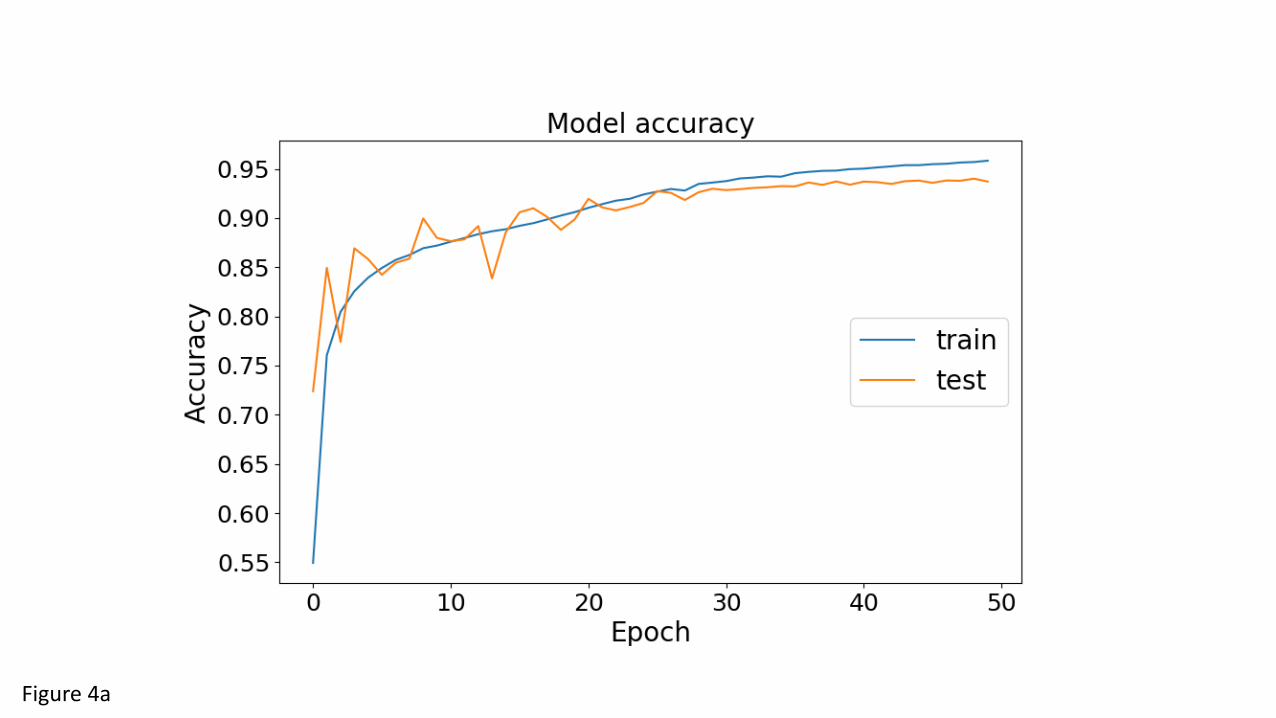
Figure 4a

Figure 4b

0.2

1.7

Tim

e (m

s)

Amp

Positive

0

Negative

Fault probability

1

0

Opacity

0.5

1 km

A A’

Figure 5a

0.2

1.7

Tim

e (m

s)A A’

Figure 5b

0.2

1.7

Tim

e (m

s)A A’

Figure 5c

1 km

A

A’

Amp

Positive

0

Negative

Fault probability

1

0

Opacity

0.5

Figure 6a

Figure 6b

0

4

Tim

e (m

s)

1 km

B B’

Amp

Positive

0

Negative

Fault probability

1

0

Opacity

0.5

Figure 7a

0

4

Tim

e (m

s)

B B’

Figure 7b

0

4

Tim

e (m

s)

B B’

Figure 7c

1 km

B

B’

Amp

Positive

0

Negative

Fault probability

1

0

Opacity

0.5

Figure 8a

Figure 8b

0

2

Tim

e (m

s)C C’

Amp

Positive

0

Negative

Fault probability

1

0

Opacity

0.5

Salt dome

Salt dome

MTD

MTD

Figure 9a

0

2

Tim

e (m

s)C C’

Figure 9b

0

2

Tim

e (m

s)C C’

Figure 9c

Salt dome

Salt dome

C C’ Amp

Positive

0

Negative

Fault probability

1

0

Opacity

0.5

1 km

MTD

Figure 10a

Figure 10b

1

3

Tim

e (m

s)

1 km

D D’

Amp

Positive

0

Negative

Fault probabilit

y1

0

Opacity

0.5

Figure 11a

1

3

Tim

e (m

s)D D’

Figure 11b

1

3

Tim

e (m

s)D D’

Figure 11c

1

3

Tim

e (m

s)D D’

Figure 11d

1 km

D D’

Figure 12a

Figure 12b

comparing convolutional neural networking and image

Documents