inelastic analysis of piping and tubular structures
TRANSCRIPT
REPORT NO.
UCBj EERC-82j 27
NOVEMBER 1982
PB<33-249987
EARTHQUAKE ENGINEERING RESEARCH CENTER
----------11--------------------------- -- -
INELASTIC ANALYSIS OF PIPINGAND TUBULAR STRUCTURES
by
MANA MAHASUVERACHAI
GRAHAM H. POWELL
Report to Sponsor:
National Science Foundation
--------~----------- -
-------I-::-If--I---I------- - --- - -
1.1-_~-A
r' . ·
------+-~--+_H_-...___l!__------- -- --
'-----------1------------- --- -
COLLEGE OF ENGINEERING
UNIVERSITY OF CALIFORNIA . Berkeley, CaliforniaREPROOUC EO BYNATIONAL TECHNICALINFORMATION SERVICE
us. DEPAR1MEHl Of COMMERCESPRiNGFiElD, VA. 22161
For sale by the National Tech nicall nformation Service, U.S. Departmentof Commerce,Springfield, Virginia 22161.
See back of report for up to date listing ofEERC reports.
DISCLAIMERAny opinions, findings, and conclusions orrecommendations expressed in this publication are those of the authors and do notnecessarily reflect the views of the NationalScience Foundation or the Earthquake Engineering Research Center, University ofCalifornia, Berkeley
INELASTIC ANALYSIS OF PIPING AND TUBULAR STRUCTURES
by
Mana MahasuverachaiGraduate Student
and
Graham H. PowellProfessor of Civil Engineering
Report toNational Science Foundationunder Grant No. CEE 8105790
Report No. UCB/EERC-82/27Earthquake Engineering Research Center
College of EngineeringUniversity of California
Berkeley, California
November 1982
l ~,, ,

ABSTRACT
Theories and computational techniques for three inelastic pipe
elements are presented. The elements can be used for inelastic stress
and deformation analysis of three-dimensional piping systems. pipelines
and tubular structures. The "fiber" procedure has been used to model
the inelastic behavior of the pipe section in all three cases. The
specific elements are as follows.
(1) A straight pipe element assuming a cubic shape function has been
developed and incorporated into the computer programs ANSR and
WIPS. This element is suitable for modeling inelastic behavior
of straight segments in piping systems, assuming closely-spaced
nodes.
(2) A curved pipe element has been developed and incorporated into
the computer programs ANSR and WIPS. This element is based on
a combination of beam and shell theories, retaining the essential
features of a beam element but introducing aspects of shell
behavior to account for cross-section ovalling. This element is
suitable for modeling inelastic behavior of curved segments in
piping systems, again assuming closely-spaced nodes.
(3) A straight pipe element which automatically determines an appro
priate shape function as the analysis progresses has been developed
and incorporated into the computer program ANSR. This is a beam
column element suitable ror modeling inelastic straight tubular
frame members, not necessarily with closely-spaced nodes.
The elements are all applicable for either small or large displace
ments analysis. The first tvlO elements also include options for the
effects of internal pressure and temperature change.
i
A number of example structures have been analyzed to test the
elements and to assess their acceptability for different applications.
These examples include: a pipeline sidebend subjected to internal
pressure and temperature changes; a pipe undergoing large displacements
following a postulated pipe rupture; and a tubular steel beam-column
with development of plastic zones near the member ends.
ii
ACKNOw~EDGEMENTS
The research described in this report was supported in part by the
National Science Foundation under Grant No. eEE 8105790 and in part by
Lawrence Livermore National Laboratory under Subcontract No. 3371609.
The authors wish to express their sincere appreciation for this support.
Sincere appreciation is also expressed to Linda Calvin for prepara
tion of the typescripts and to Gail Feazell and Mary Edmunds-Boyle for
preparation of the figures.
iii

TABLE OF CONTENTS
ABSTRACT ....
ACKNOWLEDGEMENTS
TABLE OF CONTENTS
i
iii
v
A.
B.
OBJECTIVE AND SCOPE • •
AI. INTRODUCTION .•.
Al . 1 GENERAL
Al.2 PIPE ELBOW ELEMENT
AI.3 TUBULAR BEAM-COLUMN ELEMENT
Al.4 FIBER VERSUS SECTION MODELS
A1.5 SCOPE
AI.6 REPORT LAYOUT
A2. REFERENCES
PIPE ELEMENT
Bl. INTRODUCTION.
B2. ELEMENT PROPERTIES •.
B3. CURVED ELEMENT THEORY
1
3
3
3
4
5
5
6
7
9
11
13
15
B3.I
B3.2
PROCEDURE AND ASSUMPTIONS
SLICE STIFFNESS
B3.2.1 Deformations and Actions.
B3.2.2 Subelement Strains due to Ovalling •
15
16
16
17
B3.2.3
B3.2.4
B3.2.5
B3.2.6
B3.2.7
B3.2.8
Strain-Deformation Relationships forSlice . . . . . . . . . .
Stress-Strain Relationship for SliceSubelements . . • .
Stiffness Matrix . . . . . .
Ovalling Resistance due to Pipe WallBending . . . . . • . . . .
Oval ling Stiffness due to InternalPressure . . . . . . . • . • • • • .
Condensed Slice Stiffness
18
18
19
20
21
22
B3.3 ELEMENT STIFFNESS
Preceding page blankv
23
Table of Contents (cont'd)
B3.3.1 Choice of Shape Function · · · · · 23
B3.3.2 Elastic Stiffness · · · · 23
B3.3.3 Displacement Transformation 25
B3.3.4 Element Stiffness 25
B3.4 INITIAL STRESS EFFECTS · · · · · 26
B3.4.1 General 26
B3.4.2 Pressure and Temperature Changes · 26
B3.4.3 Strain Rate Effects · · · · 27
B3.4.4 Round-Off in Mroz Material Calculations 29
B3.5 CHANGE OF SECTION GEOMETRY DUE TO OVALLING 29
B3.6 STATE DETERMINATION · · · · · 30
B4. STRAIGHT PIPE THEORY · · · · 33
B4.1 PROCEDURE AND ASSUMPTIONS 33
B4.2 SLICE STIFFNESS 34
B4.2.1 Deformations and Actions 34
B4.2.2 Strain-Deformation Relationships forSlice · · · · · · · · · · · · · 34
B4.2.3 Stress-Strain Relationships for SliceSubelement · · · · · · · 35
B4.2.4 Stiffness Matrix · · · · · 36
B4.3 ELEMENT STIFFNESS 36
B4.3.1 Deformations and Actions · · · · · 36
B4.3.2 Choice of Shape Function · 37
B4.3.3 Elastic Beam · · 37
B4.3.4 Inelastic Beam • · · · · · · · 39
B4.3.5 Internal Degrees of Freedom · · · · 39
B4.3.6 Shape Functions · · · · 39
B4.3.7 Element Stiffness · · · · · 41
B4.4 STATE DETERMINATION 42
B5. REFERENCES . . . . · · · · · · · 45
vi
Table of Contents
B6. ANSR-III USER GUIDE . 47
C. MULTI-SLICE TUBE ELEMENT . . 65
Cl. INTRODUCTION 67
Cl.l CONCEPT. 67
Cl.2 ELEMENT FEATURES 68
C2. ELEMENT PROPERTIES 69
C2.l ELEMENT GEOMETRY
C2.2 SLICE LOCATIONS.
69
69
C2.2.1
C2.2.2
C2.2.3
General •
Antisymmetrical Bending .
Other Bending Moment Variations
69
69
70
C2.3 SLICE MODELING 71
C2.4 COMPUTATIONAL PROCEDURE 71
C2.4.1
C2.4.2
Shape Function
Overshoot and Unloading Tolerances
71
72
C3. THEORY 73
C3.1 PROCEDURE AND ASSUMPTIONS • 73
C3.2 SLICE STIFFNESS .•... 74
C3.2.l Deformations and Actions 74
C3.2.2 Strain-Deformation Relationships forSlice . • . • . . • . . . • 74
· · · · 75
· · · · 76
· · · · 76
· · · · 77
77
77
. . . .
C3.4.1 Deformations and Actions
C3.2.3 Stress-Strain Relationships for SliceSubelement . . • •
C3.2.4 Stiffness Matrix
C3.4 ELEMENT STIFFNESS •
C3.4.2 Shape Function Calculation
C3.3 SLICE FLEXIBILITY.
vii
C3.5 STATE DETERMINATION ...
Table of Contents
C3.4.3
C3.4.4
C3.4.5
C3.4.6
C3.4.7
C3.4.8
C3.5.1
C3.5.2
C3.5.3
C3.5.4
C3.5.5
C4. REFERENCES
Stiffness Approach . . • • •
Weaknesses of Stiffness Approach
Flexibility Approach
Flexibility Calculation .
Shape Function
Element Stiffness
Basic Procedure .
Linearity in Mroz Material Calculations •
Linearity in Use of Shape Function
Prevention Approach .
Correction Approach •
77
79
79
80
81
81
82
82
83
83
84
86
89
D.
C5. ANSR-III USER GUIDE
EXAMPLES • . • . . .
DI. PIPE WITH AXIAL FORCE AND INTERNAL PRESSURE.
D1. I PURPOSE.
DI.2 CONFIGURATION.
91
101
103
103
103
D1.3 ANSR ANALYSIS MODEL · · · · · · 103
D1.3.I Assumptions for Analysis 103
D1.3.2 Loadings · · · · · · · · · 103
D1.3.3 ANSR Input 103
D1.4 RESULTS · . . · · · · · · · · · · · · 104
D1.5 CONCLUSION . · . . · · · · · · · · · 104
D2. BURIED PIPE BEND WITH TEMPERATURE AND PRESSURE LOADING 105
D2.I PURPOSE . . . · 105
D2.2 CONFIGURATION · · · · · · · . . . · · 105
D2.3 ANSR ANALYSIS MODEL · · · · · . . . · · · · · 105
viii
Table of Contents
D2.3.1 Assumptions of Analysis 105
D2.3.2 Loadings 105
D2.3.3 ANSR Input · · · · 106
D2.4 RESULTS · · · · · 106
D2.5 CONCLUSION · · . · . · · · · · · · · 106
D3. PIPE WHIP WITH LARGE DISPLACEMENTS 107
D3.1 PURPOSE · · · 107
D3.2 CONFIGURATION 107
D3.3 ANSR ANALYSIS MODEL · 108
D3.3.1 Geometry, Loading, and Pipe Properties 108
D3.3.2 Analysis Control Parameters · · 108
D3.3.3 ANSR Input 108
D3.4 RESULTS · · · · 109
D4. INELASTIC MULTI-SLICE BEAN COLUMN · 111
D4.1 PURPOSE · · · · . . · · · · · · 111
D4.2 CONFIGURATION · · 111
D4.3 ANSR ANALYSIS MODEL · · · · · 111
D4.3.1 Assumptions for Analysis · · · · 111
D4.3.2 ANSR Input 112
D4.4 RESULTS · · · · · . · · · · · · · · · 112
D4.4.1 Expected Behavior · · · . . 112
D4.4.2 Load Versus Deflection 112
D4.4.3 Curvature Versus Deflection · 113
D4.S CONCLUSION 114
D5. SUMMARY . . . · 115
DS.1 GENERAL · · · · · US
D6. REFERENCES · · . . 117
ix

A. OBJECTIVE AND SCOPE
This report is divided into four sections (A, B, C, and D). Section A explains the objec~
tive and scope of the research and explains the contents of Section B, C, and D.
1

At. INTRODUCTION
A1.1 GENERAL
The research described in this report is concerned with the inelastic stress and deforma
tion analysis of piping systems, pipelines and tubular structures. Specific applications which
have been considered are as follows.
(l) Analysis of pipe whip in power piping systems. The structural elements described in this
report are applicable to two- or three-dimensional pipe whip analysis, with consideration of
pipe yield, ovalling at pipe elbows, and large displacements of the piping system.
(2) Analysis of pipelines. The structural elements are applicable to both buried and above
ground pipeline systems, accounting for pipe yield, temperature changes, internal pres
sure, and large displacements.
(3) Analysis of tubular frame structures, with particular application to steel offshore plat·
forms. Analyses of piping systems and pipelines typically require that the piping be
divided into short elements, so that yielding is approximately uniform over any element.
Hence, "standard" finite element techniques using predetermined shape functions can be
applied to characterize the element behavior. For analysis of tubular frames, however, it
is desirable to use longer elements, such that the amount and location of yielding can vary
within a single element. In this case, standard finite element techniques may not work
well. To account for this problem, a new technique has been developed in which the
shape functions are updated as the analysis progresses and the state of the element
changes.
At.2 PIPE ELBOW ELEMENT
In the analysis of piping systems, it is essential to distinguish between straight and curved
segments, because a curved pipe is more flexible than a straight pipe of the same cross section.
This is due to the fact that the cross section of a curved pipe will deform (oval), which substan
tially reduces both the stiffness and strength of the pipe. Straight segments of pipe can, in
Preceding page blank3
general, be modeled adequately using straight beam-column elements with circular cross sec
tions. Curved segments are more complicated, however, and require special consideration,
especially when inelastic behavior is to be taken into account.
A commonly used procedure for the analysis of pipe bends is to use simple curved beam
theory, but with the flexural stiffness scaled by a flexibility factor to account for ovaIling [AI].
This is a simple and cheap approach, but it is applicable only for linear analysis. A more accu
rate procedure would be to use a mesh of shell finite elements to model each pipe bend. How
ever, this approach has the obvious disadvantage that computation costs are likely to be too
high for economical analysis of a complete piping system. A compromise procedure is to use
elements based on a combination of beam and shell theories, retaining the essential features of
a beam element but introducing aspects of shell behavior to account for cross-section ovalling
[A2,A3,A4]. Elements of this type can greatly reduce the computation cost compared to the
use of shell elements, while still providing good accuracy. A new element based on this
approach is described in Section B of this report.
For the special case of a straight element, the theory is substantially simpler. The straight
element theory and computational procedure are also described in Section B.
At.3 TUBULAR BEAM-COLUMN ELEMENT
In the analysis of tubular frame structures, beam-column finite elements based on
assumed cubic displaced shapes are commonly used. The use of a cubic shape function implies
a linear variation of curvature along the element length. This is correct for a uniform elastic
element but may be quite incorrect after yielding occurs. For accurate modeling, therefore, it
may be necessary to use short elements in the inelastic regions. It is generally not desirable,
however, to divide a beam-column member into short elements, because it increases the
numbers of nodes and elements which must be specified. A procedure is described in this
report which allows a long, inelastic beam-column member to be modeled accurately using a
single element. The procedure is based on varying the element shape function as the state of
the element changes, without introducing additional nodes or elements. The details of the
4
element are presented in Section C.
At." FIBER VERSUS SECTION MODELS
Two basic procedures may be used for modeling the inelastic behavior of a beam-column.
In the "section" type of model it is assumed that inelastic behavior is defined for the cross sec
tion as a whole, whereas in the "fiber" type of model the member cross section is divided into a
number of small areas (fibers). In the section model, stiffness and strength properties are
specified for the complete section, and only the stress and strain resultants need to be moni
tored. In the fiber model, properties are defined for the fibers, and the stresses and strains in
each fiber must be monitored. The fiber model thus tends to be more expensive computation
ally. However, the calculation of cross section properties for the section model may be a
difficult task, so that the fiber model tends to be both easier to use and more accurate.
For the pipe elbow element described in Section B, only the fiber type of model is
appropriate, whereas the beam-column theory described in Section C is applicable to either the
section or fiber type of model. In this report, however, only a fiber model has been developed,
for the particular casse of a tubular cross section. Other elements could be developed following
similar principles.
AI.S SCOPE
The purpose of the study described in this report has been to explore theoretical and com
putational techniques for modeling inelastic straight and curved pipe members using the "fiber"
type of model. Three separate elements have been developed, as follows.
(1) A straight pipe element assuming a cubic shape function has been developed and incor
porated into the computer programs ANSR-III [AS] and WIPS [A6]. This element is suit
able for modeling inelastic behavior of· straight segments in piping systems, assuming
closely-spaced nodes.
5
(2) A curved pipe element has been developed and incorporated into the computer programs
ANSR and WIPS. This element is suitable for modeling inelastic behavior of curved seg
ments in piping systems, again assuming closely-spaced nodes.
(3) A straight pipe element which automatically determines an appropriate shape function as
the analysis progresses has been developed and incorporated into the computer program
ANSR. This element is suitable for modeling inelastic straight tubular frame members,
not necessarily with closely-spaced nodes.
The elements are all applicable for either small or large displacements. The first two ele
ments include options for internal pressure and temperature change effects, making them suit
able for inelastic analysis of pipelines and piping systems. The third element has been
developed in only a preliminary form. Further work is needed on this element to add practical
features.
Al.6 REPORT LAYOUT
Section B presents the theory of the inelastic straight and curved pipe elements. Section
C presents the inelastic beam-column element for tubular frames. Both sections have been
written as self-contained reports. Examples using all three of the elements are contained in
Section D.
6
A2. REFERENCES
AI. Dodge, W. G. and Moore, S. E., "Stress Indices and Flexibility Factors for Moment Loadings on Elbows and Curved Pipes," Welding Research Council Bulletin 179, December1972.
A2. Marcal, P. V., "Elastic-Plastic Behavior of Pipe Bend with In-Plane Bending," J. StrainAnalysis, Vol. 2, No.1, pp. 84·96, 1967.
A3. Hibbitt, H. D., Sorensen, E. P., and Marcal, P. V., "The Elastic-Plastic and Creep Analysisof Pipelines by Finite Elements," in Pressure Vessel Technology, Pt. 1, ASME, pp. 239251, 1973.
A4. Ohtsubo, H. and Watanabe, 0., "Stress Analysis of Pipe Bend by Ring Elements," Trans.ASME, Ser. J, Vol. 100, pp. 112-122, 1978.
AS. Oughourlian, C. V., "General Purpose Computer Program for Nonlinear StructuralAnalysis," Ph.D. Thesis, Department of Civil Engineering, University of California, Berkeley, 1982.
A6. Powell, G. H., Hollings, J. P., Row, D. G., Chen, P. F-S., Hu, F-e., Mahasuverachai, M.,Mosaddad, B., Nicklin, P., Nour-Omid, S., Oughourlion, C. and Riahi, A., "WIPS - Computer Code for Whip and Impact Analysis of Piping Systems," Report to Lawrence Livermore National Laboratory, 1982.
7

B. PIPE ELEMENT
This section describes the theory of the straight-curved pipe element. The basic features of
the element are described in Chapters BI and B2. Details of the theory and computational pro
cedure are described in Chapter B3 for a curved (elbow) element and in Chapter B4 for a
straight element. Chapter BS contains references, and Chapter B6 describes the input data
required for the ANSR-III computer code.
Preceding page blank
9

BI. INTRODUCTION
The pipe type element has the following features.
(1) The element may be straight or curved, and arbitrarily oriented in space.
(2) If the element is straight, it is treated as a three-dimensional beam column. Inelastic
behavior is considered by dividing the cross section into subelements (or fibers), and
monitoring the behavior of each subelement. Longitudinal, circumferential, and torsional
stresses are considered.
(3) If the element is curved, it is similar in many respects to a straight element, but includes
additional deformations to account for ovalling. A number of simplifying assumptions are
made in developing the ovalling theory.
(4) The Mroz material model is used, with allowance for strain rate dependence if desired.
(5) The effects of internal pressure on ovalling stiffness and material yield are considered.
(6) Large displacement effects may be considered, if desired, using an engineering theory (j.e.
not a consistent continuum mechanics approach).
A general description of the element properties is presented in Chapter B2. Theoretical
details for the curved element are presented in Chapter B3 and for the straight element in
Chapter B4.
Preceding page blank
11
82. ELEMENT PROPERTIES
Beam-column finite elements based on assumed cubic displaced shapes are commonly
used for elastic and inelastic analysis. The straight pipe element is exactly of this type, and the
curved pipe element is essentially of this type. However, there are several complicating factors
introduced when the element is curved rather than straight. The assumptions and properties
are described in physical terms in this chapter. Full theoretical details are presented in Chapters
B3 and B4.
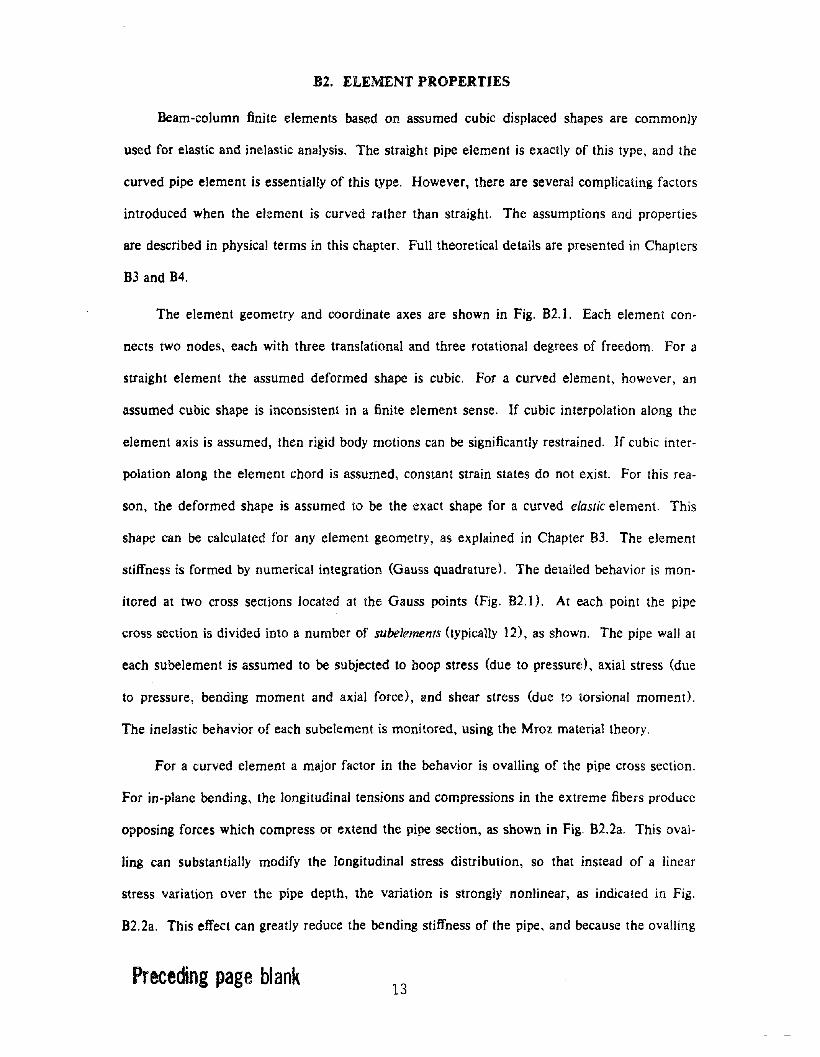
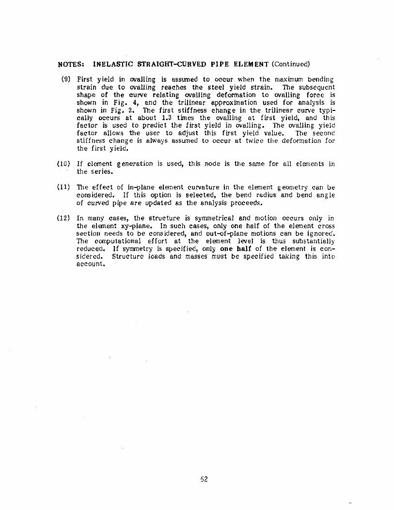
The element geometry and coordinate axes are shown in Fig. B2.1. Each element con
nects two nodes, each with three translational and three rotational degrees of freedom. For a
straight element the assumed deformed shape is cubic. For a curved element, however, an
assumed cubic shape is inconsistent in a finite element sense. If cubic interpolation along the
element axis is assumed, then rigid body motions can be significantly restrained. If cubic inter
polation along the element chord is assumed, constant strain states do not exist. For this rea
son, the deformed shape is assumed to be the exact shape for a curved elastic element. This
shape can be calculated for any element geometry, as explained in Chapter B3. The element
stiffness is formed by numerical integration (Gauss quadrature). The detailed behavior is mon
itored at two cross sections located at the Gauss points (Fig. B2.0. At each point the pipe
cross section is divided into a number of subelements (typically 12), as shown. The pipe wall at
each subelement is assumed to be subjected to hoop stress (due to pressure), axial stress (due
to pressure, bending moment and axial force), and shear stress (due to torsional moment>.
The inelastic behavior of each subelement is monitored, using the Mroz material theory.
For a curved element a major factor in the behavior is ovalling of the pipe cross section.
For in-plane bending, the longitudinal tensions and compressions in the extreme fibers produce
opposing forces which compress or extend the pipe section, as shown in Fig. B2.2a. This avaI
ling can substantially modify the longitudinal stress distribution, so that instead of a linear
stress variation over the pipe depth, the variation is strongly nonlinear, as indicated in Fig.
B2.2a. This effect can greatly reduce the bending stiffness of the pipe, and because the availing
Preceding page blank13
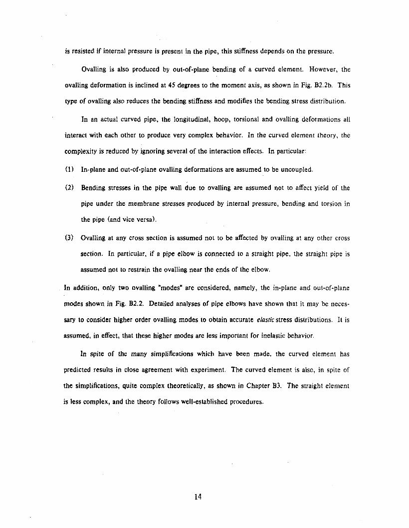
is resisted if internal pressure is present in the pipe, this stiffness depends on the pressure.
OvaIling is also produced by out-of-plane bending of a curved element. However, the
ovalling deformation is inclined at 45 degrees to the moment axis, as shown in Fig. B2.2b. This
type of ovalling also reduces the bending stiffness and modifies the bending stress distribution.
In an actual curved pipe, the longitudinal, hoop, torsional and ovaIling deformations all
interact with each other to produce very complex behavior. In the curved element theory, the
complexity is reduced by ignoring several of the interaction effects. In particular:
(l) In-plane and out-of-plane ovalling deformations are assumed to be uncoupled.
(2) Bending stresses in the pipe wall due to ovaIling are assumed not to affect yield of the
pipe under the membrane stresses produced by internal pressure, bending and torsion in
the pipe (and vice versa).
(3) OvalJing at any cross section is assumed not to be affected by ovaIling at any other cross
section. In particular, if a pipe elbow is connected to a straight pipe, the straight pipe is
assumed not to restrain the ovalling near the ends of the elbow.
In addition, only two ovalling "modes" are considered, namely, the in-plane and out-of-plane
modes shown in Fig. B2.2. Detailed analyses of pipe elbows have shown that it may be neces
sary to consider higher order ovaIling modes to obtain accurate elastic stress distributions. It is
assumed, in effect, that these higher modes are less important for inelastic behavior.
In spite of the many simplifications which have been made, the curved element has
predicted results in close agreement with experiment. The curved element is also, in spite of
the simplifications, quite complex theoreticallY, as shown in Chapter B3. The straight element
is less complex, and the theory follows well-established procedures.
14
B3. CURVED ELEMENT THEORY
B3.1 PROCEDURE AND ASSUMPTIONS
The stiffness and state determination calculations for the element are based on a combina
tion of beam and shell theory.
The element is modelled as shown in Fig. B3.I. At each of the two Gauss integration
points a beam slice is considered, and each slice is divided into a number of cross-section subele
ments. The subelement stiffnesses are constructed first, allowing for elasto-plastic behavior of
the pipe steel. The slice stiffnesses are constructed from the subelement stiffnesses by summa
tion. The complete element stiffness is then constructed from the slice stiffnesses by Gauss
quadrature.
The slice deformations consist of six beam-type deformations plus two ovalling deforma
tions. The beam deformations consist of axial deformation, torsional twist, in-plane and out
of-plane curvatures, and in-plane and out-of-plane flexural shear deformations. One ovaIling
deformation is associated with in-plane bending, and the second with out-of-plane bending (Fig.
B3.2).
The beam deformations at each slice are related to the element node displacements by a
deformation shape function. The ovalling deformations in any slice are assumed to be indepen
dent of the ovalling deformations at other slices. Hence, no shape function is assumed for vari
ation of ovalling along the element length. The ovaIling deformations are internal degrees of
freedom at each slice and are condensed out before the element stiffness is constructed from
the slice stiffnesses.
Each subelement is assumed to be in a state of plane stress, with axial, hoop, and shear
stresses. The axial strain in any subelement is affected by axial deformation and curvature of
the slice and by the ovalling deformations. The effects of axial deformation and curvature are
determined assuming plane (but not necessarily circular) cross sections. The effects of availing
are determined using the membrane equations for an axisymmetric shell. The shear strain in
15
any subelement is assumed to be affected by torsional twist only. Flexural shear effects are
assumed to be negligible at the subelement level and are ignored <they are introduced at the
slice level). The subelement shear strains due to twist are determined assuming plane, circular
cross sections.
Hoop strains are not determined from strain-displacement relationships. Rather, the hoop
stresses are governed by the equilibrium relationship between internal pressure and hoop stress.
The hoop strain in any subelement thus becomes an internal degree of freedom for the subele
ment and is condensed out before the slice stiffness is constructed.
The hoop stress in equilibrium with the internal pressure is the average value over the
pipe wall thickness. In addition, ovalling induces pipe wall bending, and hence stresses which
vary through the pipe wall thickness. It is assumed that yielding of slice subelements is not
affected by pipe wall bending, and correspondingly that flexural yield of the pipe wall due to
ovalling is not affected by subelement yield. That is, it is assumed that membrane and bending
effects in the pipe wall are uncoupled.
Although it is not essential to the theory, it is assumed that the centerline radius of the
bend is large compared with the pipe radius. This is not generally true for piping elbows. How
ever, in view of the many other assumptions made in developing the theory, this assumption is
believed to be reasonable. Ford and Turner [Bll have shown that the assumption produces
only small errors.
B3.2 SLICE STIFFNESS
B3.2.! Deformations and Actions
The slice deformation vector is ~s, given by
~! -= < 8 '" n 'Y II '" r 'Y r q, W II W r > (B3.0
in which 8 "" axial strain at pipe axis; q, co rate of torsional twist; '" n -= in-plane bending cur-
vature; '" r 0::: out-of-plane bending curvature; 'Y II 0::: in-plane flexural shear deformation; 'Y r =
out-of-plane flexural shear deformation; W II 0::: in-plane ovaIling (Fig. B3.2); and w, = out-of-
16
plane ovalling.
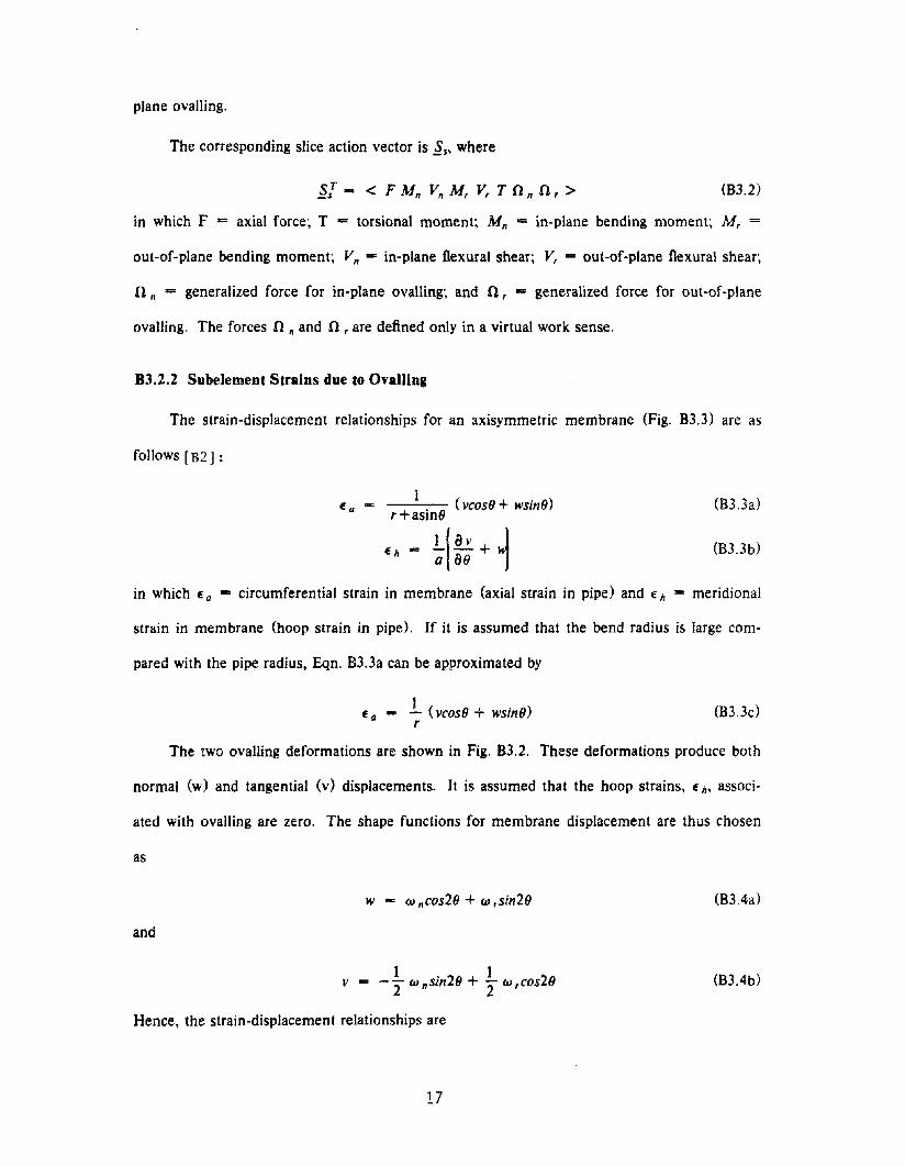
The corresponding slice action vector is J.s, where
J.I.. < F M n VnM, V, T n nn, > (B3.2)
in which F ... axial force~ T ... torsional moment; M n .... in-plane bending moment; M, =
out-of-plane bending moment~ V" -= in-plane flexural shear; V, ... out-of-plane flexural shear;
n n = generalized force for in-plane ovaIling; and n r ... generalized force for out-of-plane
ovalling. The forces n " and n , are defined only in a virtual work sense.
B3.2.2 Subelement Strains due to Ovalling
The strain-displacement relationships for an axisymmetric membrane (Fig. B3.3) are as
follows [B2] :
E a .. 1 ( vcos9 + wsin9)r+asin9
Eh ... i[!! + .Ja 89 1
(B3.3a)
(B3.3b)
in which E a ... circumferential strain in membrane (axial strain in pipe) and E h = meridional
strain in membrane (hoop strain in pipe). If it is assumed that the bend radius is large com-
pared with the pipe radius, Eqn. 83.3a can be approximated by
E a - 1 (vcos9 + wsin9)r
(B3.3d
The two ovalling deformations are shown in Fig. 83.2. These deformations produce both
normal (w) and tangential (v) displacements. It is assumed that the hoop strains, E h, associ-
ated with ovalling are zero. The shape functions for membrane displacement are thus chosen
as
w .. w "cos29 + w ,sin29
and
v .. - ~ w"sin29 + ~ w,cos29
Hence, the strain-displacement relationships are
17
(B3.4a)
(B3.4b)
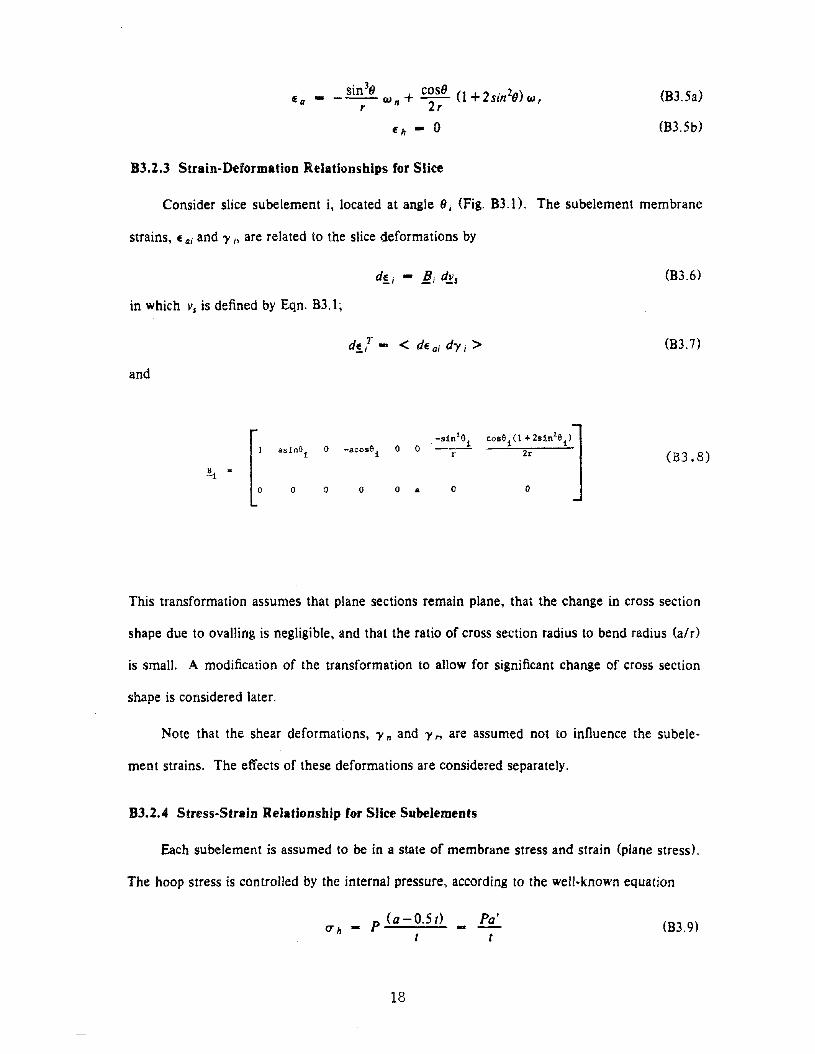
sin3(J + cos9 (1 +2 . 2.a)
iii a - - -- w -- Sin 17 W,r n 2r
Eh - 0
B3.2.3 Strain-Deformation Relationships for Slice
(B3.5a)
(B3.5b)
Consider slice subelement i, located at angle 9; (Fig. B3. I). The subelement membrane
strains, iii aj and')' ;, are related to the slice deformations by
(B3.6)
in which Vs is defined by Eqn. B3.1;
(B3.7)
and
[:asin6
10 -acos6
10 0
-sin 361 '0" , (I "",0".']
r 2r (B3.8)8 •-1
0 0 0 0 a 0 0
This transformation assumes that plane sections remain plane, that the change in cross section
shape due to ovalling is negligible, and that the ratio of cross section radius to bend radius (aIr)
is small. A modification of the transformation to allow for significant change of cross section
shape is considered later.
Note that the shear deformations, ')' nand ')'" are assumed not to influence the subele-
ment strains. The effects of these deformations are considered separately.
B3.2.4 Stress-Strain Relationship for SUce Subelements
Each subelement is assumed to be in a state of membrane stress and strain (plane stress).
The hoop stress is controlled by the internal pressure, according to the well-known equation
p (a-O.5t) _
t
18
Pa't
(B3.9)
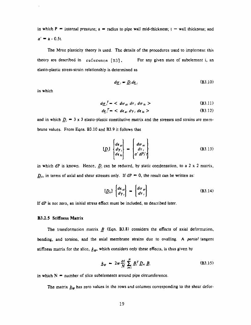
in which P .. internal pressure; a "'" radius to pipe wall mid-thickness; t = wall thickness; and
a' IE a • 0.5t.
The Mroz plasticity theory is used. The details of the procedures used to implement this
theory are described in reference [B3].
elasto-plastic stress-strain relationship is determined as
For any given state of subelement i, an
in which
du t - < du ai d'T i du hi >d!J - < dE ai dy i dE hi >
(B3.10)
(B3.1 I)
(B3.12)
and in which 12i .. 3 x 3 elasto-plastic constitutive matrix and the stresses and strains are mem-
brane values. From Eqns. 83.10 and B3.9 it follows that
IdE ail Idu ai J[D,] dy, ,dT I
dE hi a dP/(B3.13)
in which dP is known. Hence, Di can be reduced, by static condensation, to a 2 x 2 matrix,
Drio in terms of axial and shear stresses only. If dP -= 0, the result can be written as:
[D] IdE ail IdU ail-" dy I dT I
If dP is not zero, an initial stress effect must be included, as described later.
B3.2.5 Stiffness Matrix
(B3.14)
The transformation matrix ~ (Eqn. B3.8) considers the effects of axial deformation,
bending, and torsion, and the axial membrane strains due to ovaIling. A partial tangent
stiffness matrix for the slice, .!ssp, which considers only these effects, is thus given by
(B3.15)
in which N .. number of slice subelements around pipe circumference.
The matrix .!ssp has zero values in the rows and columns corresponding to the shear defor-
19
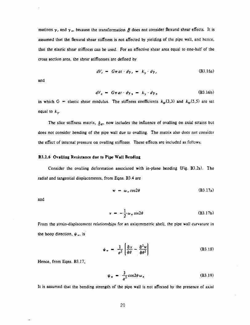
mations ')', and ')' n' because the transformation B does not consider flexural shear effects. It is
assumed that the flexural shear stiffness is not affected by yielding of the pipe wall, and hence,
that the elastic shear stiffness can be used. For an effective shear area equal to one-half of the
cross section area, the shear stiffnesses are defined by
dV, - G'IT at . d')', .., ky ' d')',
and
(B3.16a)
(B3.16b)
in which G ... elastic shear modulus. The stiffness coefficients kspO,3) and ksp(S,S) are set
equal to k y •
The slice stiffness matrix, .!ssp, now includes the influence of ovalling on axial strains but
does not consider bending of the pipe wall due to ovalling. The matrix also does not consider
the effect of internal pressure on ovalling stiffness. These effects are included as follows.
B3.2.6 Ovalling Resistance due to Pipe Wall Bending
Consider the ovalling deformation associated with in-plane bending (Fig. B3.2a). The
radial and tangential displacements, from Eqns. B3.4 are
W ... W n cos29
and
(B3.17a) .
v ... (B3.17b)
From the strain-displacement relationships for an axisymmetric shell, the pipe wall curvature in
the hoop direction, t/1 w, is
Hence, from Eqns. B3.17,
3t/1w ... -2coslOw n(J
(B3.18)
(B3.19)
It is assumed that the bending strength of the pipe wall is not affected by the presence of axial
20
and hoop membrane stresses. Hence, for any given steel stress-strain relationship, a moment-
curvature relationship can be determined for the pipe wall. For a given state of strain at loca-
tion (J on the pipe wall, let the moment-curvature relationship be
Hence, from Eqns. B3.19 and B3.20, a generalized ovalling stiffness can be defined by
9 2trdO hn ... 4 f cos226 . I .., . ad6 . dW n
a 0
or
dO hn ... kwh dW n
(B3.20)
(B3.21a)
(B3.21b)
By integrating around the pipe circumference, the relationship between 0 hn and W n can be
determined. When normalized to 0 lOy'" 1 and wiwy ... 1, where 0 y and wy = values at first
yield, the relationship depends on the steel stress-strain curve but is independent of the ratio of
pipe radius to wall thickness.
The normalized O-w relationships have been calculated for three different stress-strain
curves, as shown in Fig. B3.4. It can be seen that the shapes of the curves do not vary greatly.
Hence, for any given stress-strain curve, the !l-w relationship can be estimated from Fig. B3.4
without evaluating Eqn. B3.21.
For analysis, a trilinear relationship is assumed, as shown in Fig. B3.5. The same trilinear
relationship is used for both in-plane and out-of-plane ovalling, and it is further assumed that
the ovalling deformations W nand w, are uncoupled. Hence, the ovalling stiffness, kwh' is
added to the diagonal terms ksp (7,7) and ksp (8,8) of the slice stiffness matrix.
B3.2.7 Oulling Stiffness due to Internal Pressure
The equilibrium relationship between internal pressure and hoop stress is given by Eqn.
B3.9. This assumes that the pipe radius, a, remains constant. As the cross section ovals, how-
ever, the pipe radius changes, with the result that for constant hoop stress an equilibrium error
develops. This error can be regarded as an unbalanced internal pressure, which tends to resist
21
availing.
Consider in-plane Dvalling, W n (Fig. B3.2a). From Eqn. B3.19, the change in hoop curva-
ture at location 9 in the pipe wall is
3t/J '" .., -2cos29w n
o
Hence, the unbalanced pressure, Pu, is given by
Pu - Un tt/J", .., P{o - 0.5r) t/J ..
(B3.22)
(B3.23 )
in which P = internal pressure. Assuming tla is small, it follows from Eqns. B3.23 and B3.22
that
3PP .., - cos28wu 0 n
Hence, the generalized force associated with P", is given by
3P 2...n -= - f cos 228 . od8 . wpn 0 n
o
or
n pn ... 3PfTW n - k wp W n
(B3.24)
(B3.25a)
<B3.25b)
It is assumed that the same stiffness applies for both in-plane and out-of-plane ovalling and that
the stiffnesses are uncoupled. Hence, the stiffness kwp is added to the diagonal terms ksr (7.7)
and ksp{8,8) of the slice stiffness.
B3.2.8 Condensed Slice Stiffness
After addition of the ovalling stiffnesses, the partial slice stiffness, !ssp, becomes the slice
stiffness, .!ss. The ovalling deformations are assumed to be internal degrees of freedom for the
slice. Hence, the 8 x 8 matrix can be condensed to a 6 x 6 matrix, !5" in terms of the stress
resultants on the pipe cross section.
22
B3.3 ELEMENT STIFFNESS
B3.3.1 Choice of Shape Function
For straight beam elements, it is common to use a cubic shape function. For a curved
beam, however, the use of a cubic function may lead to substantial errors. For this reason, a
shape function is constructed which is exact for an elastic curved beam element, and this same
shape function is assumed also to apply for the inelastic element. The determination of the
shape function requires additional calculation. However, this calculation is performed only
once, at the beginning of the analysis, and does not add significantly to the total cost. The pro-
cedure is as follows.
B3.3.2 Elastic Stiffness
Consider an elastic curved beam, with nodal degrees of freedom as shown in Fig. B3.6.
The 12 nodal displacements can be transformed to 6 symmetric-antisymmetric deformation pat-
terns (Fig. B3.7) plus 6 rigid-body displacements. The elastic stiffness in terms of the
symmetric-antisymmetric deformations can be obtained in closed form as follows.
The equilibrium relationship between the slice stress resultants and the symmetric-
antisymmetric generalized forces is
in which
§! - < F M n Vn M, V, T >NT - < N) N2 N) N4 Ns N6 >
(B3.26)
(B3.27)
(B3.28)
o cosB -5 inB1rs in¢
r(casB-cos¢> -s1nBlsin4>(B3.29)
o sinS cosB/rsin¢
cosB sinB -cos¢sinB
23
o
-sinB
o
casB
-l/rsin¢
I - cospc~sint
and f3 (positive or negative) defines the slice location (Fig. B3.7).
The elastic slice flexibility is defined by
1's, .., Is §s,
in which
.il: ... < 81/1n 'Yn 1/1, 'Yr f/J >
and
. [1 1 2 1 2 11Is ... d,ag EA aEi GA aEI GA 2GI
(B3.30)
(B3.31)
(B3.32)
in which E = Young's modulus; G r.= shear modulus; A == cross section area; 1 = cross sec-
tion moment of inertia; and a = flexibility factor to account for ovaIling. The flexibility factor
follows from the ovaIling theory described in the preceding sections (from the reduced slice
stiffness, iss" for the elastic case, determine the effective EI value). The result is
9a -= 1 - -------,i-...".....----
10 + -!l- [..!!...]2 + 48Pr2
1-1I2 a2 Eat
(B3.33)
in which v = Poisson's ratio. The flexibility factor given by the well-known von Karman
theory [B41 is (for P=O)
a ... 1 - -1O-+-1-:~I-;~--:1"""'2
which is essentially identical to Eqn. B3.33.
(B3.34)
(B3.35)
From Eqns. B3.26 and B3.30, the element 6 x 6 flexibility matrix, EN, in symmetric-
antisymmetric coordinates follows as
EN ... 112'k Is 12N rd(3-<$>
in which rand (3 are defined in Fig. B3.7. The flexibility coefficients can be obtained by closed
form integration. The matrix EN uncouples into two 2 x 2 plus two 1 x 1 submatrices, so that
only 8 coefficients need to be evaluated.
24
The element stiffness, K N, in symmetric-antisymmetric coordinates is easily obtained by
inverting IN.
B3.3.3 Displacement Transformation
The deformations at a slice, ~sr, can be obtained as follows.
From Eqns. B3.30 and B3.26
(B3.36)
Hence,
~sr - [s ~N K N 11 - En 11 (B3.37)
in which 11 contains displacements corresponding to fl. A transformation between the
symmetric-antisymmetric deformations and the 12 local displacements (Fig. B3.6a) can easily be
constructed. This can then be combined with the well,known coordinate rotation transforma-
tion from local to global displacements, 1, (Fig. B3.6b). A combined transformation between
symmetric-antisymmetric deformations and global displacements follows in the form
n - a r- -'-Hence, from Eqn. B3.37,
<B3.38)
(B3.39)
Matrix E.sr is the required transformation between nodal displacements and slice deformations.
B3.3.4 Element Stiffness
The transformation matrix, !ls" is formed for each slice (Gauss poind in the element.
The element stiffness then follows as
K - ~ W i !ll!sr E.srj
in which Wi - Gauss quadrature weighting function and !sr is the 6 x 6 slice stiffness.
25
(B3.40)
83.4 INITIAL STRESS EFFECTS
B3.4.1 General
The effects of loads which originate at the element level are treated as initial stress effects.
Pipe elements can, in general, be subjected to initial stresses due to changes in temperature,
changes in internal pressure, and creep. Loads which originate at the element level are also
introduced when rate-dependent plasticity is considered. Temperature, pressure, and creep pro-
duce real initial stresses, with physical meanings. The initial stresses caused by strain rate
effects exist only in a mathematical sense.
Initial stresses affect the analysis in two ways. First, they contribute to the load vector;
and, second, they influence the state determination calculatiQn. Initial stresses do not affect the
stiffness calculation.
B3.4.2 Pressure and Temperature Cbanges
At a slice subelement, i, the tangent stress-strain relationship, including initial stress
effects, is
(B3.41)
in which dP .... pressure increment, dT .... temperature increment, and a .... coefficient of ther-
mal expansion. Eqn. 83.41 can be condensed to the form
Idf7 DII_ [Df/] IdE Dil + Idf7 DOlidT I dy I dT 01
or
df!..ri - Dr; d!.i + df!..or;
(B3.42)
(B3.43)
Application of the procedures of Section B3.2 produces the slice stiffness relationship
~s - lis d~s + ~so
in which lss is as defined in Section B3.2.8, and
2'ITot';' T~so - -N ~!li df!..or; +
i..1
26
'IT a'2
ooooooo
(B3.44)
(B3.45)
is the initial slice force. The last term in this equation is the axial force in the contained fluid
(pipe inside area times fluid pressure). Because the increment of slice ovalling forces is zero,
Eqn. B3.44 can be condensed to the form:
~sr - ksr d~sr + ~sor (B3.46)
By the procedure of Section B3.3, this relationship can be transformed to the following relation-
ship in symmetric-antisymmetric coordinates:
dN - K N dn + dNa
in which !i,!J. and K N are as defined in Section B3.3.3, and
dNa - I. Wi.!l!: ~sorii
(B3.47)
(B3.48)
in which Wi == Gauss weighting factor at slice i and the transformation En is defined by Eqn.
B3.37. Finally, dNa is transformed to global coordinates using the transformation of Eqn.
B3.38.
B3.4.3 Strain Rate Effects
The general theory for material strain rate dependence has been presented by Mosaddad
[B3]. Certain additional assumptions have been made in applying this theory to the pipe ele-
ment. A summary of the assumptions is as follows.
(a) It is assumed that strain rate effects influence only the membrane stresses. The bending
stiffness of the pipe wall is assumed to be rate independent.
(b) Strain increments are divided into elastic and plastic components:
d! - d!e + d!p
(c) Stress increments are divided into plastic and damping components:
du - du p + d!!..d
(d) Total stress increments and elastic strain increments are related by Hooke's law:
27
(B3.49)
(B3.50)
(B3.5})
(e) Mroz effective plastic stress increments are related to effective plastic strain increments by
the rate-independent Mroz model:
• T •dcr p... !!u dcr p- Kde p (B3.52)
(B3.53)
in which du; .... effective plastic stress increment; dE; ..., effective plastic strain incre
ment; n! == unit vector normal to the yield surface; and K == tangent plastic modulus.
(f) The damping stress increment is defined by:
dcrd'" C [~/!p-!pl
in which C .... damping coefficient, dt ..., time step, and !p is the plastic strain rate. This
equation assumes that the backward difference integration scheme is used.
(g) The flow rule is defined by:
(B3.54)
With these assumptions, the governing equations are obtained as follows. Premultiply
Eqn. B3.50 by!!! and substitute Eqns. B3.52 - B3.54 into Eqn. B3.50 to get the effective
plastic strain increment as:
• n! dcr + C!!! f. p
dE p ... K + C/dt
By virtue of Eqns. B3.51, B3.54, and B3.55, Eqn. B3.49 can be written as:
I
nn T I Cn TidE'" D-1 + _u_u dcr + _u p n- _f K + C/ dt - K + C/ dt _u
Inversion of Eqn. B3.56 by the Sherman-Morrison formula results in:
in which
and
28
(B3.55)
(B3.56)
(B3.57)
(B3.58)
(B3.59)
(B3.60)
For a finite time step, dt is replaced by A t. The last term in Eqn. B3.57, deY 0" is then treated
as an initial stress. In each time step, the initial stresses, deY or' are transformed to initial ele-
ment forces and assembled into the effective load vector for the step.
83.4.4 Round-Off in Mroz Material Calculations
In the state determination calculation for the Mroz material, the stresses calculated assum-
ing linear behavior are scaled so that the stress point lies exactly on the yield surface. This
means that the calculated hoop stress in any slice subelement may not exactly satisfy Eqn. B3.9.
If this error is not corrected, it may accumulate over a number of load increments and reach a
significant magnitude.
The error is corrected by determining, for each subelement, the internal pressure
corresponding to the calculated hoop stress. The difference between this pressure and the
actual pressure is then a pressure error. At each iteration, this value is added to dP in Eqn.
83.41 and treated as an initial stress effect. This prevents accumulation of error.
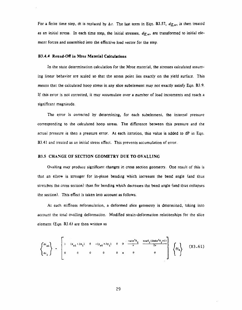
83.5 CHANGE OF SECTION GEOMETRY DUE TO OVALLING
Ovalling may produce significant changes in cross section geometry. One result of this is
that an elbow is stronger for in-plane bending which increases the bend angle (and thus
stretches the cross section) than for bending which decreases the bend angle (and thus collapses
the section). This effect is taken into account as follows.
At each stiffness reformulation, a deformed slice geometry is determined, taking into
account the total availing deformation. Modified strain-deformation relationships for the slice
element (Eqn. 83.6) are then written as
(Xoi
+lIxi
) 0 -(yoi +t.yi) 0. -sin 3S
i ,...,',.....,.,'"!{~}
0--2rr (B3.61)
0 0 0 0 a 0 0
29
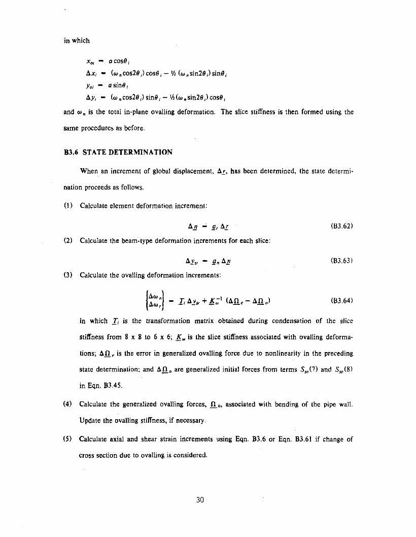
in which
xo; - acosO;
ax; - (w n cos20 ;) cosO; - Ih (w n sin20 ;) sinO;
Yo; - a sinO;
/1y; - (w n cos20 ;> sinO; - Ih (w n sin20 ;) cosO;
and W n is the total in-plane ovalling deformation. The slice stiffness is then formed using the
same procedures as before.
B3.6 STATE DETERMINATION
When an increment of global displacement, /1L, has been determined, the state determi-
nation proceeds as follows.
(I) Calculate element deformation increment:
/111 ... fir aL
(2) Calculate the beam-type deformation increments for each slice:
/1~sr - En al!(3) Calculate the ovalling deformation increments:
(B3.62)
(B3.63)
(B3.64)
in which I; is the transformation matrix obtained during condensation of the slice
stiffness from 8 x 8 to 6 x 6; K", is the slice stiffness associated with ovalling deforma
tions; /10 e is the error in generalized ovaIling force due to nonlinearity in the preceding
state determination; and a 0 0 are generalized initial forces from terms Sso (7) and Sso (8)
in Eqn. B3.45.
(4) Calculate the generalized ovalling forces, 0 h, associated with bending of the pipe wall.
Update the ovalling stiffness, if necessary.
(5) Calculate axial and shear strain increments using Eqn. B3.6 or Eqn. B3.61 if change of
cross section due to ovaIling is considered.
30
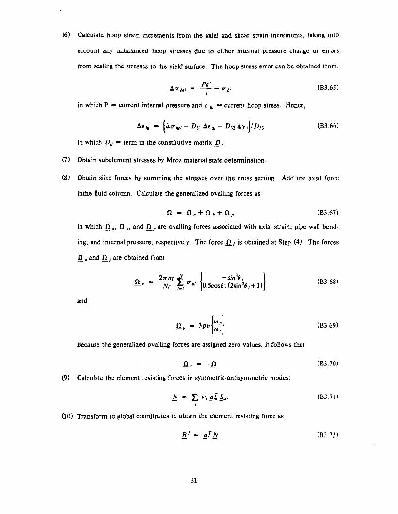
(6) Calculate hoop strain increments from the axial and shear strain increments, taking into
account any unbalanced hoop stresses due to either internal pressure change or errors
from scaling the stresses to the yield surface. The hoop stress error can be obtained from:
Po'IiCT ~-' - -- - CT h'"", t '
in which P ... current internal pressure and (T hi - current hoop stress. Hence,
liE hi - (IiCT hei - D 31liE ai - D n liy i)1 D33
in which Dij ... term in the constitutive matrix Di •
(7) Obtain subelement stresses by Mroz material state determination.
(B3.65)
(B3.66)
(8) Obtain slice forces by summing the stresses over the cross section. Add the axial force
inthe fluid column. Calculate the generalized ovalling forces as
(B3.67)
in which n a, 0 h, and n pare ovalling forces associated with axial strain, pipe wall bend-
ing, and internal pressure, respectively. The force 0 h is obtained at Step (4). The forces
o a and 0 p are obtained from
27Tat ~Oa ... -N L" CTai
r i-I
and
I -sin3() , I
O.5cos(} i (2sin2() i + 1)(B3.68)
Because the generalized ovalling forces are assigned zero values, it follows that
o --0_e _
(9) Calculate the element resisting forces in symmetric-antisymmetric modes:
N -. I. Wi E! ~srii
(to) Transform to global coordinates to obtain the element resisting force as
31
(B3.69)
(B3.70)
(B3.70
(B3.72)

B4. STRAIGHT PIPE THEORY
B4.1 PROCEDURE AND ASSUMPTIONS
The stiffness and state determination calculations for the element are based essentially on
beam theory.
The element can be modeled as either a "Gauss slice" model (Fig. B4.1a) or as an "end
slice" model (Fig. B4.1 b). For WIPS, the default option is the Gauss model. At each of the
two integration points, a beam slice is considered, and each slice is divided into a number of
cross section sube/ements. The subelement stiffnesses are constructed first, allowing for elasto
plastic behavior of the pipe steel. The slice stiffnesses are constructed from the subelement
stiffnesses by summation. The complete element stiffness is then constructed from the slice
stiffnesses by either Gauss quadrature (for the Gauss model) or by closed form integration (for
the end slice model).
The slice deformations consist of six beam type deformations, namely axial deformation,
torsional twist, in-plane and out-of-plane curvatures, and in-plane and out-of-plane flexural
shear deformations.
The complete element has six nodal degrees of freedom at each end (Fig. B4.2), which
provide six rigid body modes plus six element deformations. In addition, two internal degrees
of freedom are considered to allow linear variation of axial strain and torsional twist along the
element length. These degrees of freedom are added to avoid excessive constraint by allowing
linear strain variation along the element axis. A typical beam formulation allows only constant
strain, which is reasonable if the element axis is also the centroidal axis of the beam. In an ine
lastic element, however, the effective centroidal axis will shift as the cross section yields.
The slice deformations are related to the element deformations by shape functions which
include the effects of shear deformation. Each subelement of a slice is assumed to be in a state
of plane stress, with axial, hoop, and shear stresses. The effects of axial deformation and cur
vature on axial strains are determined assuming plane, circular cross sections. The shear strain
Preceding page blank33
is assumed to be affected by torsional twist only. Flexural shear effects are assumed to be
negligible at the subelement level and are ignored (they are introduced at the slice level). The
subelement shear strains due to twist are determined assuming plane, circular cross sections.
Hoop strains ,are not determined from strain-displacement relationships. Rather the hoop
stresses are governed by the equilibrium relationship between internal pressure and hoop stress.
The hoop strain in any subelement thus becomes an internal degree of freedom for the subele-
ment and is condensed out before the slice stiffness is constructed.
B4.2 SLICE STIFFNESS
B4.2.1 Deformations and Actions
The slice deformation vector, .!is' is given by:
(B4.D
in which 8 -= axial strain at pipe axis; l/J z -= bending curvature about element z axis; l/J y =
bending curvature about y axis; cP = rate of torsional twist; ')' xy == flexural shear deformation in
x-y plane; and')' xz == flexural shear deformation in x-z plane.
The corresponding slice action vector is §s, where
(B4.2)
in which F -= axial force; Mz and My .. bending moments; T .... torsional moment; and Vxy
and VXI ... flexural shear forces.
B4.2.2 Strain-Deformation Relationships for Slice
Consider slice subelement i, located at angle 9 i (as for a curved element, Fig. B3.D. The
subelement membrane strains, E oi and 'Y it are related to the slice deformations by:
in which .!'s is defined by Eqn. B4.1;
dE,r - < dE .d')'·>_I _01 ,
34
(B4.3)
(B4.4)
and
B [1 asin9; -acos9 i 0 0 oj_i - 0 0 0 a 0 0 (84.5)
This transformation assumes that plane sections remain plane and circular. It is also implied
that the pipe thickness is small compared to the pipe diameter.
Note that the slice shear deformations, 'Y xy and 'Y xz, are assumed not to influence the
subelement strains. The efl"ects of these deformations are considered separately.
84.2.3 Stress-Strain Relationships for Slice Subelement
Each subelement is assumed to be in a state of membrane stress and strain (plane stress).
The hoop stress is controlled by the internal pressure, according to the well-known equation
p (a-0.5t) Pa'CTh - --t t
(84.6)
in which P ... internal pressure; a ... radius to pipe wall mid-thickness; t ... wall thickness; and
a' = a - 0.51.
The Mroz plasticity theory is used. The details of the procedures used to implement this
theory have been described by Mosaddad [B3J and are not repeated here. For any given state
of subelement i, an elasto-plastic stress-strain relationship is determined as
in which
dfL T - < dCT ai dr i dCT hi >d!r - < deOi dYi dE hi >
(84.7)
(B4.8)
(B4.9)
and in which 12; -= 3 x 3 elasto-plastic constitutive matrix and the stresses and strains are mem-
brane values. From Eqns. 84.7 and 84.6 it follows that
IdE all IdCT 01 J12, - d*'Y i - dT,dE hi a/tiP/
(B4.1O)
in which dP is known. Hence, Di can be reduced, by static condensation, to a 2 x 2 matrix,
35
Dr;, in terms of axial and shear stresses only. If dP -= 0, the result can be written as:
[D .1IdEail_ldO' ail_f1 d')'i dTj
If dP is not zero, an initial stress effect must be included, as described later.
B4.2.4 Stiffness Matrix
(B4.10
The transformation matrix lJ. (Eqn. B4.5) considers the effects of axial deformation,
bending, and torsion. A tangent stiffness matrix for the slice, Bs, which considers only these
effects, is thus given by:
(B4.12)
in which N -= number of slice subelements around pipe circumference.
The matrix Bs has zero rows and columns corresponding to the shear deformations ')' xy
and')'=, because the transformation !l does not consider flexural shear effects. It is assumed
that the flexural shear stiffness is not affected by yielding of the pipe wall, and hence, that the
elastic shear stiffness can be used. For an effective shear area equal to one-half of the cross
section area, the shear stiffnesses are defined by:
dVxy .. G'Tr at • d')' xy .. k'Y' d')' xy
and
(B4.13a)
(B4.13b)
in which G -= elastic shear modulus. The stiffness coefficients ks(5,5) and ks(6,6) are set
equal to k'Y'
B4.3 ELEMENT STIFFNESS
84.3.1 Deformations and Actions
The element degrees of freedom, after deletion of the six rigid body modes, are given by:
<84.14)
36
in which Ux == axial extension; (J zi == z-axis rotation at element end i; (J zj = z-axis rotation at
end j; (J x .. torsional twist; 9yi .. y-axis rotation at end i; () y) .. y-axis rotation at end j; Uxm =
additional axial degree of freedom at element midpoint (displacement relative to the element
ends); and (J xm == additional torsional deformation at element midpoint (twist relative to ele
ment ends).
The corresponding element action vector is §.m' where
§! - <Fx M zi Mzj Tx M yi My) Fxm Txm > (B4.15)
The forces Fxm and Txm are defined only in a virtual work sense and are assigned zero values.
B4.3.2 Choice of Shape Function
For straight beam elements, it is common to use a cubic hermitian polynomial shape
function, which is exact for a uniform elastic beam. If shear deformations are included, the
shape can no longer be obtained from kinematic considerations only. Rather the equilibrium
relationship between moments and shears must be considered, with the result that the shape
function depends on the ratio of the flexural and shear stiffnesses. If a shape function is deter
mined using the elastic stiffness values, then when the beam becomes inelastic it is implied that
the ratio between the flexural and shear stiffnesses remains constant. This is unlikely to be
correct. A more reasonable assumption, in general, is that the flexural stiffness changes
whereas the shear stiffness remains constant. This assumption is made for the formulation of
the slice stiffness and must be retained at the element level to avoid inconsistencies. For this
reason, the shape function is continually updated as the analysis proceeds, using a strain energy
minimization procedure as follows.
84.3.3 Elastic Beam
A shape function is "exact" if it satisfies both the homogeneous governing equation for
the element and the displacement boundary conditions at the element ends. An important pro
perty of an exact shape function is that it corresponds to a strain energy which is an "absolute"
minimum.
37
For a uniform elastic beam element loaded only at its ends, the governing equation is a
homogeneous fourth order differential equation, and the exact displaced shape is at most cubic.
If shear deformations are ignored, the exact shape is the well-known cubic hermitian polyno-
miaI. If shear deformations are considered, the exact shape can be obtained by solving the
differential equation directly, or alternatively by using a linear combination of polynomials up to
cubic and choosing the combination factors to minimize the strain energy.
For a finite element formulation, the alternative method is preferable. Consider a uni-
form beam in which both flexural and shear deformations are present. Impose a unit rotation
at the end x .... 0, with the end x -= L fixed (Fig. B4.3a). The beam will have bending defor-
mation plus a constant shear deformation, y. If vex) defines the transverse displacement of
the beam axis, the boundary conditions are:
v(O) ... 0
V'(O} 1 - y
vel) 0
v'(L) ... -y
A combination of cubic and quadratic polynomials which satisfies these boundary conditions is:
I 2x2 x3! 1-(' [ ~Ivex) .. c x - - + - + -- x - -
L L 2 2 L
in which
c ... 1 - 2y
The strain energy of the beam is:
L
U .. lhf EJ( v"(x»2d.x + Ih GA L(y xy)2o
(B4.16)
(B4.17)
(B4.18)
Substitution of Eqns. B4.16 and B4.17 into Eqn. B4.18, and minimization with respect to c
results in:
in which
c -
38
(B4.19)
4 L [6 31Q - f £1 2._ - dx - 01 GA'L2 0 L2 L
and
(B4.20)
1 [ )2
4 £1 6x 3 dx131 - GA'L 2 0 7}- T.
These equations define the shape function.
B4.3.4 Inelastic Beam
12£/GA'L 2
(B4.2D
For an inelastic beam, the stiffness along the element length can vary, and hence, the
governing differential equation is generally not known. Thus, it is not generally possible to
obtain the shape function by a closed form solution. A simple and effective procedure is to
apply strain energy minimization with certain assumptions. In Eqn. B4.l6, the shape function
depends on the ratio of flexural stiffness to shear stiffness. As an approximation, the diagonal
terms of the slice stiffness matrix are assumed to define effective flexural stiffnesses, and the
slice shear stiffnesses are assumed to remain constant. The shape function is then obtained, as
described in Section B4.3.6.
84.3.5 Internal Degrees of Freedom
The two internal degrees of freedom, Uxm and 8 xm' are included to allow for linear varia-
tion of axial and torsional deformations along the element axis. The shape functions associated
with these degrees of freedom do not involve flexural or shear deformations. No strain energy
is associated with these deformations because the corresponding generalized forces are assigned
zero values.
B4.3.6 Shape Functions
Displacement shape functions relating element deformations to the longitudinal,
transverse, and twisting displacements along the element are obtained by strain energy minimi-
zatian. They can be expressed as:
Idu(x)Idv(x) _ N(x) dvdw(x) - _mdf/>(x)
39
(B4.22)
in which u .. longitudinal displacement; v and w .. transverse displacements in the y and z
directions, respectively; tb .. twist; and N is given by:
in which
xlL 0o N22o 0o 0
o 0 0 0N23 0 0 0o 0 N35 N36o xl L 0 0
N17 0o 0o 0o N48
(B4.23)
N48 - -4x2
+ 4xL
~:;: [x- 2t + ~:I+ ~~:;:) [x- ~l:~;: I~ - ~ 1+ ~;:;:) [~ -1::;; (x- 2t +~: 1+ ~~~;:) [x- ~ l~:;: I~~-II + ~~:;:) [I -1
The shape functions relating the element degrees of freedom to the slice deformations are
obtained by differentiating the displacement shape functions. They can be expressed as:
in which d,£s and d'£m are defined by Eqns. B4.1 and B4.14, and
(84.24)
IlL 0 0 0 0 0 -8q 0
0 8 22 8 23 0 0 0 0 0
0 0 0 0 8 35 8 36 0 0 B4.25).! .
0 0 0 llL 0 0 0 -8q
0 8 52 8 530 0 0 0 0
0 0 0 0 8 65 8 66 0 0
in which the transformation £ is defined in terms of dimensionless coordinates q (Fig. B4.3b)
as:
40
-6(l+a z}q+ 1;°22 (l+fjz)
-6(I-a z}q-1;023 - (I+fj z)
-6(l+ay}035 (I+fj) q + 1;
-6(I-a }036 - (I+{3J q-1;
({3z-a z)052 ..
20+{3z) L;
({3 z+a z)053 2(I+{3z} L;
({3y-a y)065 - 20+{3y} L;
({3y+a y)066 - 2(I+fjy) L;
lh
24 fa z 'L2 k/2,2} q dqGA -'h
'h
f3z - G~4,~2 £k s(2,2) q2 dq
'h24 fa y '2 ks(3,3) q dq
GA L -'h
'h
f3y .. 144 J ( ) 2GA'L 2 -lh ks 3,3 q dq
For the Gauss model, the integrals are obtained by Gauss quadrature. For the end slice model,
the integrals are evaluated in closed form, assuming that ks (2,2) and ks (3,3) vary linearly
along the element length.
The shape function is updated at each element stiffness reformulation. If shear deforma-
tions are ignored, reformulation is not necessary.
B4.3.7 Element Stiffness
For the Gauss model, the shape function, f!, is formed at each slice (Gauss point) in the
element. The element stiffness then follows as:
K - ~ W oT k· °_ ,l,. I _I _SI_'
i
(B4.26)
in which Wi -= Gauss quadrature weighting function at slice i, and isSi is the 6 x 6 stiffness at
41
slice i.
For the end slice model, the element stiffness is calculated assuming that the slice
stiffness, .5." varies linearly along the element length. Hence, the element stiffness can be
obtained by closed form integration as:
'h
K - L f 11 T !s 11 dq-'h
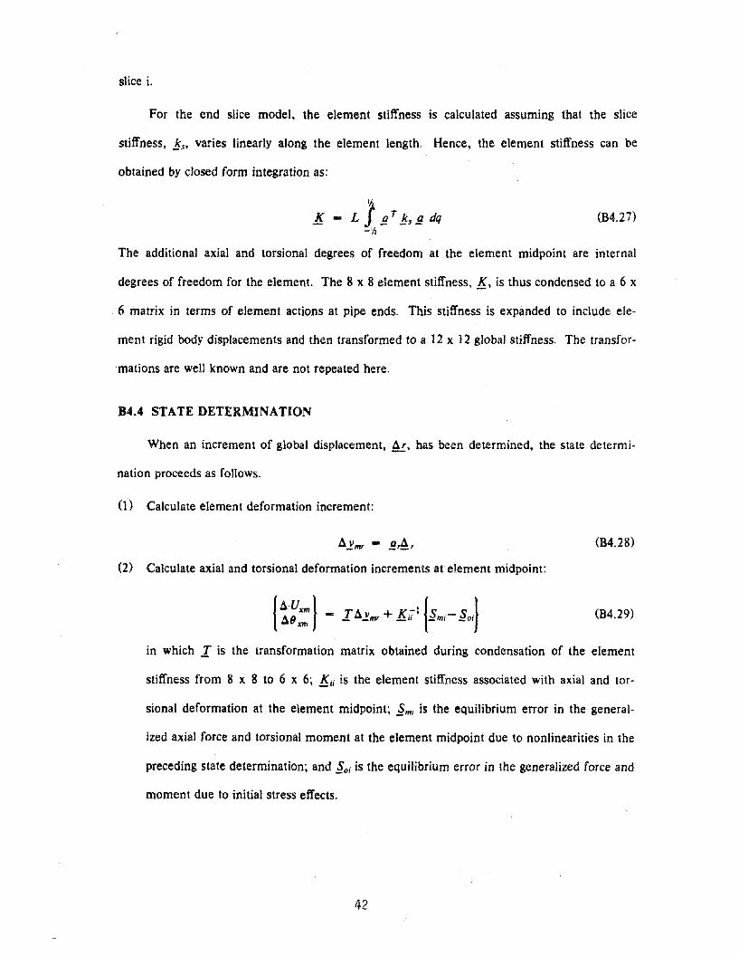
(B4.27)
The additional axial and torsional degrees of freedom at the element midpoint are internal
degrees of freedom for the element. The 8 x 8 element stiffness, K, is thus condensed to a 6 x
6 matrix in terms of element actions at pipe ends. This stiffness is expanded to include ele-
ment rigid body displacements and then transformed to a 12 x 12 global stiffness. The transfor-
mations are well known and are not repeated here.
B4.4 STATE DETERMINAnON
When an increment of global displacement, t:.,. has been determined. the state determi-
nation proceeds as follows.
(I) Calculate element deformation increment:
(B4.28)
(2) Calculate axial and torsional deformation increments at element midpoint:
(B4.29)
in which I is the transformation matrix obtained during condensation of the element
stiffness from 8 x 8 to 6 x 6; K ii is the element stiffness associated with axial and tor-
sional deformation at the element midpoint; ~mi is the equilibrium error in the general-
ized axial force and torsional moment at the element midpoint due to nonlinearities in the
preceding state determination; and ~Oi is the equilibrium error in the generalized force and
moment due to initial stress effects.
42
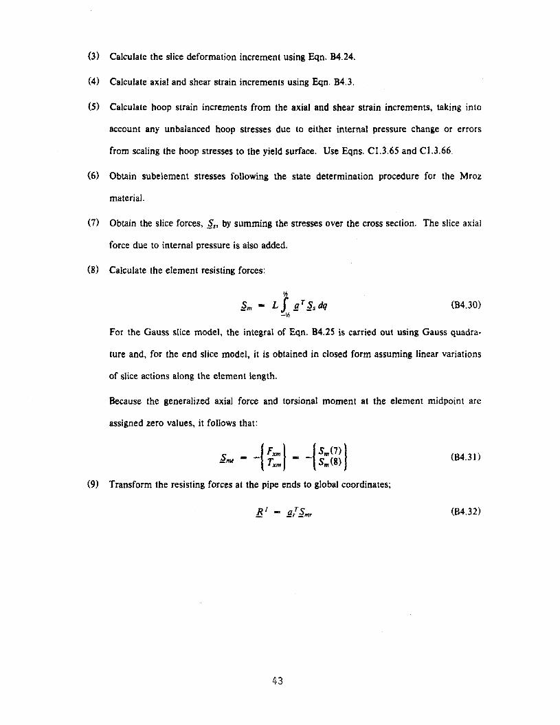
(3) Calculate the slice deformation increment using Eqn. B4.24.
(4) Calculate axial and shear strain increments using Eqn. B4.3.
(S) Calculate hoop strain increments from the axial and shear strain increments, taking into
account any unbalanced hoop stresses due to either internal pressure change or errors
from scaling the hoop stresses to the yield surface. Use Eqns. C1.3.6S and C1.3.66.
(6) Obtain subelement stresses following the state determination procedure for the Mroz
material.
(7) Obtain the slice forces, §s, by summing the stresses over the cross section. The slice axial
force due to internal pressure is also added.
(S) Calculate the element resisting forces:
'h
§m - L f !l T§s dq-'h
(B4.30)
For the Gauss slice model, the integral of Eqn. 84.25 is carried out using Gauss quadra-
ture and, for the end slice model, it is obtained in closed form assuming linear variations
of slice actions along the element length.
Because the generalized axial force and torsional moment at the element midpoint are
assigned zero values, it follows that:
(B4.31)
(9) Transform the resisting forces at the pipe ends to global coordinates;
(B4.32)
43

BS. REFERENCES
B1. Turner and Ford, "Examination of the Theories for Calculating the Stresses in Pipe BendsSubjected to In-Plane Bending," Proc. Ins!. Mech. Engrs., Vol. 171, pp. 513-525,1957.
B2. Timoshenko, S. P. and Woinowsky, S., Tbeory of Plates and Sbells, McGraw-Hill, 1959.
B3. Mosaddad, B., "Computational Models for Cyclic Plasticity, Rate Dependence and Creep,"Ph.D. Thesis, Civil Engineering Department, University of California, Berkeley, June1982.
B4. Von Karman, T., "Uber die Formauderung Dunnwanndiger Rohre," InnsbesonIngenieure, Vol. 55, pp. 1889-1895, 1911.
Preceding page blank45

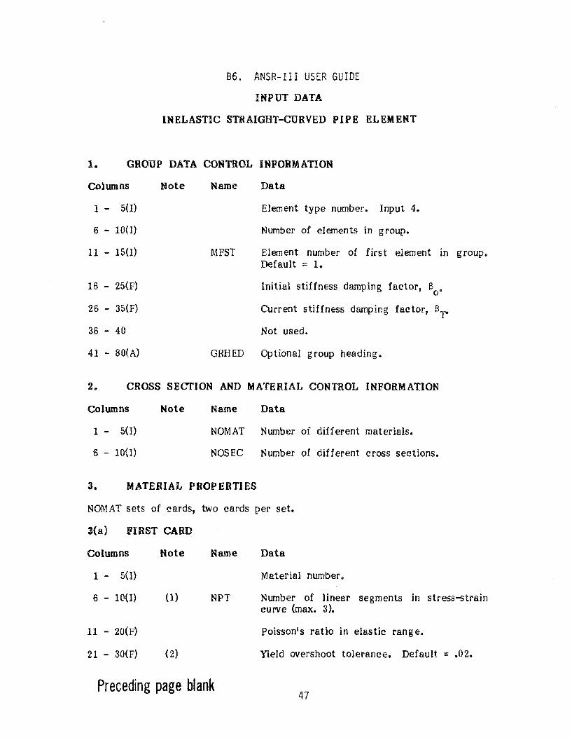
86. ANSR-III USER GUIDE
INPUT DATA
INELASTIC STRAIGHT-CURVED PIPE ELEMENT
1. GROUP DATA CONTROL INFORMATION
Columns
1 - 5(1)
6 - 10(1)
11 - 15(1)
16 - 25(F)
26 - 35(F)
36 - 40
Note Name
MFST
Data
Element type number. Input 4.
Number of elements in group.
Element number of first element in group.Default =1.
Initial stiffness damping factor, 80
•
Current stiffness damping factor, BT"
Not used.
41 - 80(A) GRHED Optional group heading.
2. CROSS SECTION AND MATERIAL CONTROL INFORMATION
Columns Note Name Data
1 - 5(1)
6 - 10(1)
NOM AT Number of different materials.
NOSEC Number of different cross sections.
3. MATERIAL PROPERTIES
NOMAT sets of cards, two cards per set.
3(8) FIRST CARD
Columns
1 - 5(1)
6 - 10(1)
11 - 20(F)
21 30(F)
Hote
(l)
(2)
Name
NPT
Data
Material number.
Number of linear segments in stress-straincurve (max. 3).
poisson's ratio in elastic range.
Yield overshoot tolerance. Default = .02.
Preceding page ~ank47
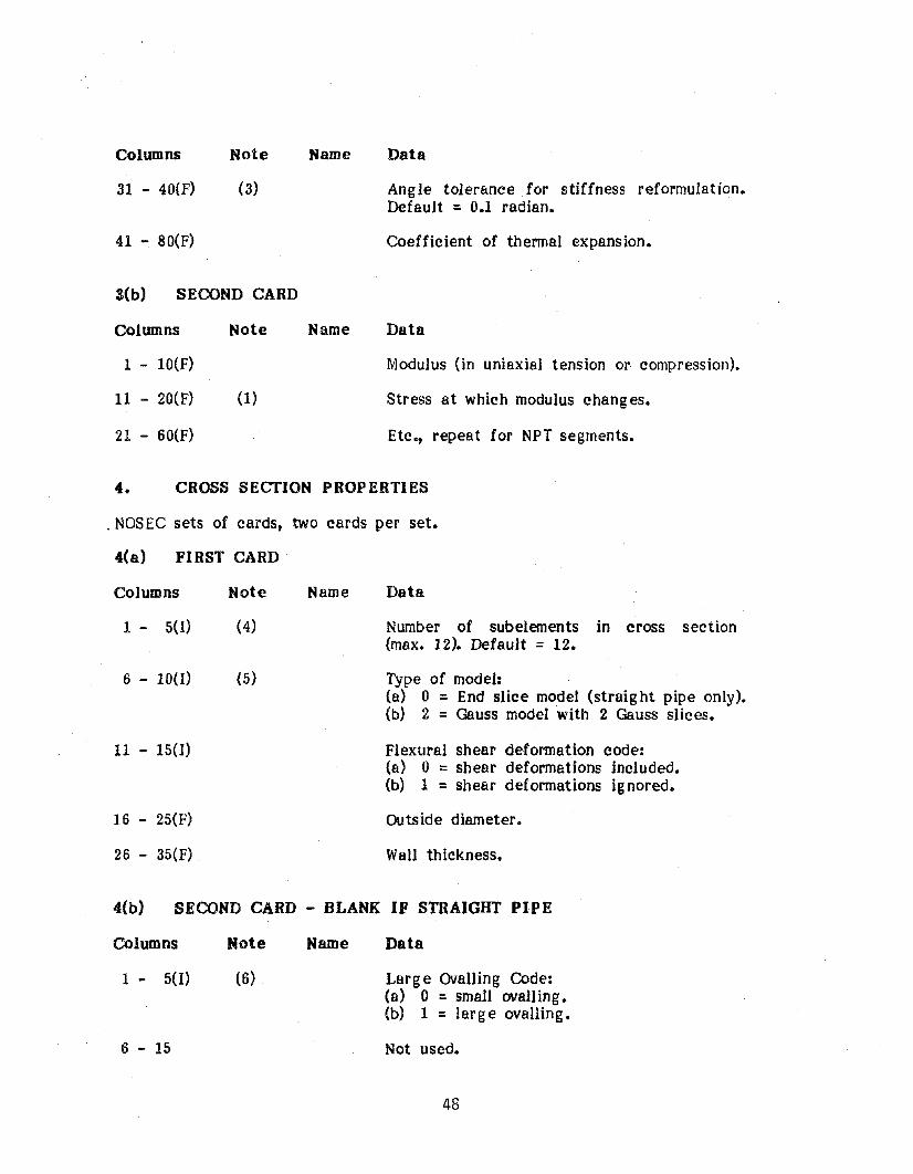
Columns
31 - 40(F)
41 - 80(F)
Note Name Data
Ang Ie tolerance. for stiffness reformulation.Default = 0.1 radian.
Coefficient of thermal expansion.
3(b) SECOND CARD
Columns
1 - 10(F)
11 - 20(F)
21 - 60(F)
Note
(1)
Name Data
Modulus (in uniaxial tension or compression).
Stress at which modulus changes.
Etc., repeat for NPT segments.
4. CROSS SECfION PROPERTIES
. NOSEC sets of cards, two cards per set.
4(a) FIRST CARD
Columns
1 - 5(1)
6 - 10(1)
11 - 15(1)
16 - 25(F)
26 - 35(F)
Note
(4)
(5)
Name Data
Number of subelements in cross section(max. 12). Default = 12.
Type of model:(a) 0 = End slice model (strai ght pipe only).(b) 2 = Gauss model with 2 Gauss slices.
Flexural shear deformation code:(a) 0 =shear deformations included.(b) 1 =shear deformations ignored.
Outside diameter.
Wall thickness•
.f(b) SECOND CARD - BLANK IF STRAIGHT PIPE
Columns
1 - 5(1)
6 - 15
Note
(6)
Name Data
Large avaIling Code:(a) 0 =small ovalling.(b) 1 =large ovaUing.
Not used.
48
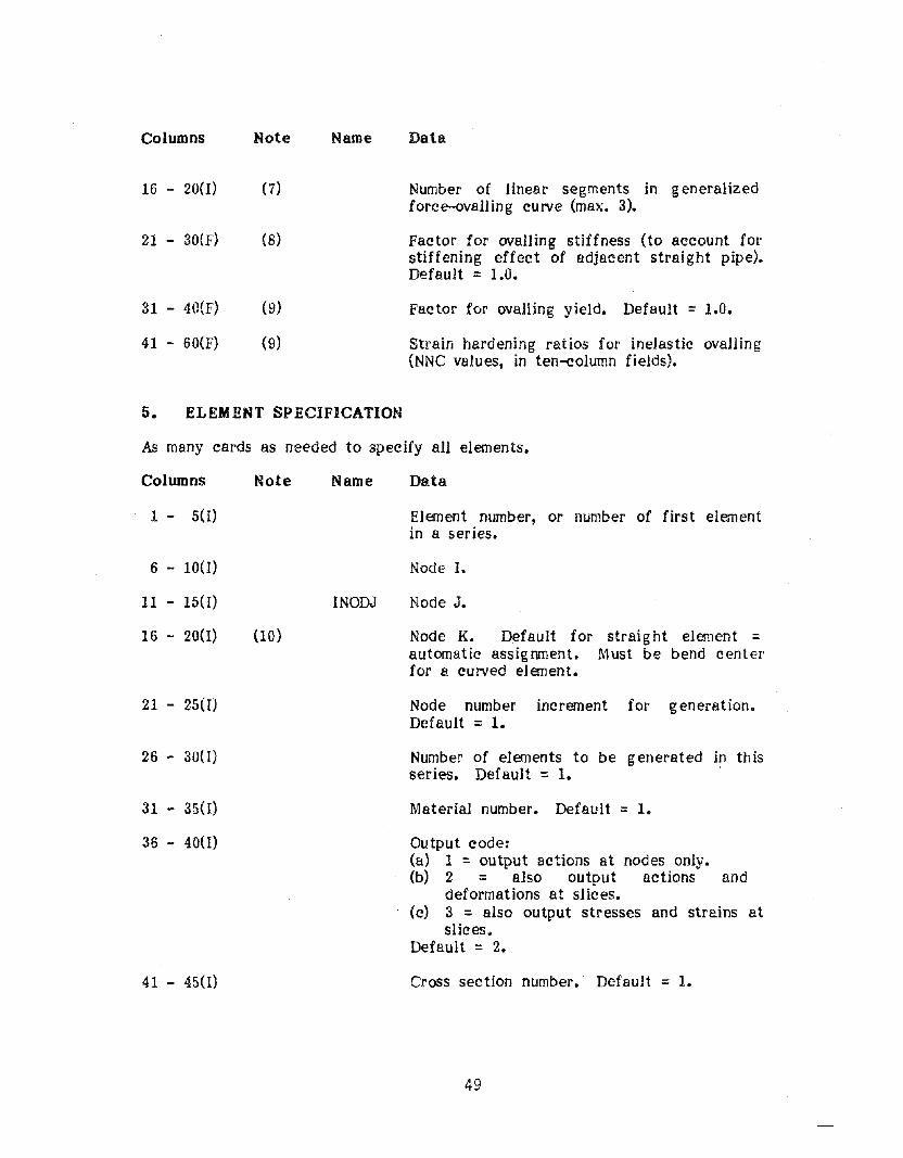
Columns
16 - 20(1)
21 - 30(F)
31 - 40(F)
41 - 6o(F)
Note
(7)
(8)
Name Data
Number of linear segments in generalizedforce-ovalling curve (max. 3).
Factor for ovaIling stiffness (to account forstiffening effect of adjacent straight pipe).Default :: 1.0.
Factor for ovalling yield. Default = 1.0.
Strain hardening ratios for inelastic ovalling(NNe values, in ten-column fields).
5. ELEMENT SPECIFICATION
As many cards as needed to specify all elements.
Columns
1 - 5(I)
6 - 10(1)
11 - 15(1)
16 - 20(1)
21 - 25(1)
26 - 300)
31 - 35(1)
36 - 40(1)
41 - 45(0
Note
(10)
Name
{NODJ
Data
Element number, or number of first elementin a series.
Node I.
Node J.
Node K. Default for straight element =automatic assignment. Must be bend centerfor a curved element.
Node number increment for generation.Default =1.
Number of elements to be generated in thisseries. Default:: 1.
Material number. Default = 1.
Output code:(a) 1 = output actions at nodes only.(b) 2 = also output actions and
deformations at slices.(c) 3 = also output stresses and strains at
slices.Default = 2.
Cross section number. Default = 1.
49
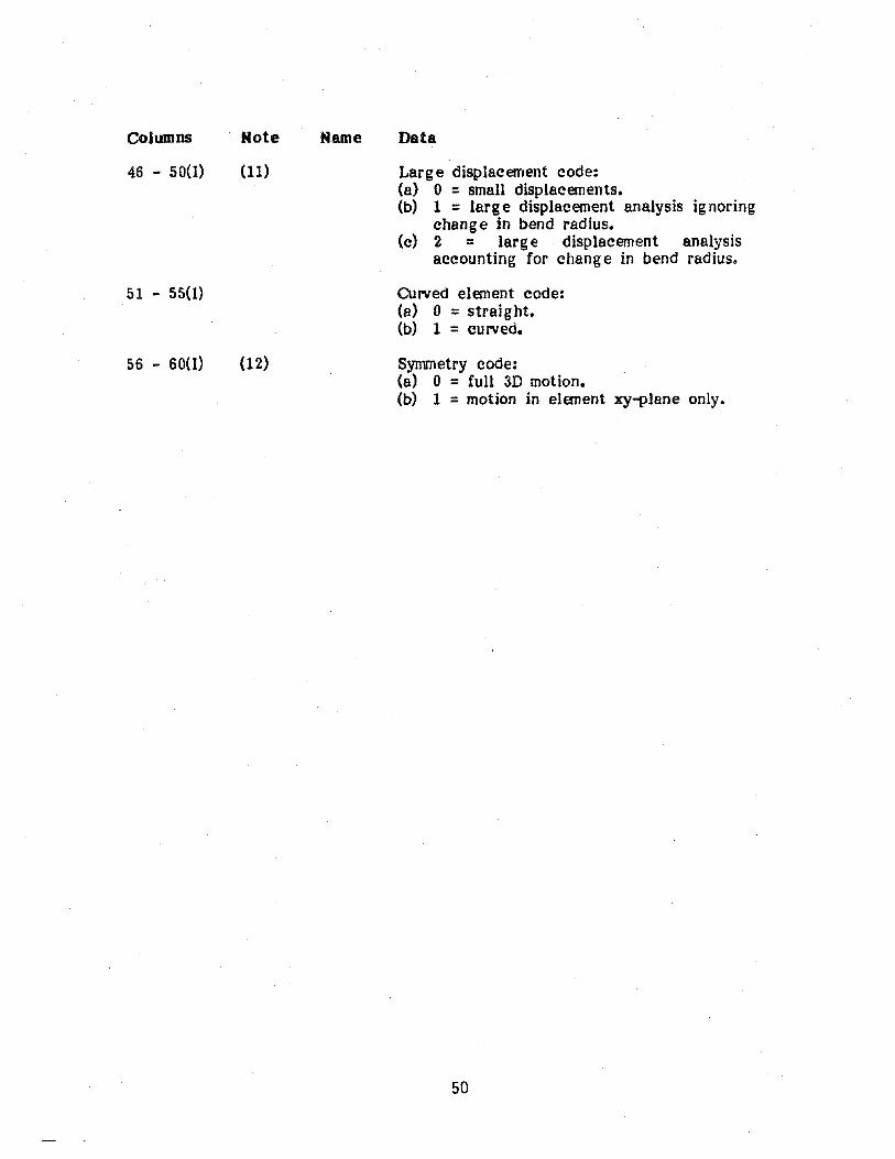
Columns
46 - 50(1)
51 - 55(1)
56 - 60(1)
Note
(11)
(12)
Name Data
Large displacement code:(a) 0 = small displacements.(b) 1 =large displacement analysis ignoring
change in bend radius.(c) 2 = larg e displacement analysis
accounting for change in bend radius.
Curved element code:(a) 0 =straight.(b) 1 = curved.
Symmetry code:(a) 0 =full 3D motion.(b) 1 =motion in element xy-plane only.
50
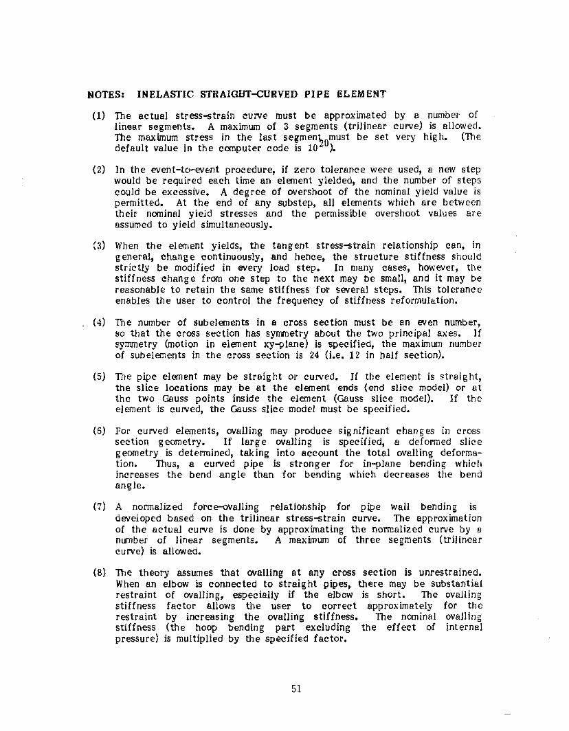
NOTES: INELASTIC STRAIGHT-CURVED PIPE ELEMENT
(1) The actual stress-strain curve must be approximated by a number oflinear segments. A maximum of 3 segments (trilinear curve) is allowed.The maximum stress in the lastsegmen~omust be set very hig h. (Thedefault value in the computer code is 10 ).
(2) In the event-tcr~event procedure, jf zero tolerance were used, a new stepwould be required each time an element yielded, and the number of stepscould be excessive. A degree of overshoot of the nominal yield value ispermitted. At the end of any substep, all elements which are betweentheir nominal yield stresses and the permissible overshoot values areassumed to yield simUltaneously.
(3) When the element yields, the tangent stress-strain relationship can, ingeneral, chang e continuously, and hence, the structure stiffness shouldstrictly be modified in every load step. In many cases, however, thestiffness change from one step to the next may be small, and it may bereasonable to retain the same stiffness for several steps. This toleranceenables the user to control the frequency of stiffness reformulation.
. (4) The number of subelements in a cross section must be an even number,so that the cross section has symmetry about the two principal axes. Ifsymmetry (motion in element xy-plane) is specified, the maximum numberof sub elements in the cross section is 24 (i.e. 12 in half section).
(5) The pipe element may be straight or curved. If the element is straight,the slice locations may be at the element ends (end slice model) or atthe two Gauss points inside the element (Gauss slice model). If theelement is curved, the Gauss slice model must be specified.
(6) For curved elements, ovaIling may produce significant changes in crosssection geometry. If large ovalling is specified, a deformed slicegeometry is determined, taking into account the total ovaIling deformation. Thus, a curved pipe is stronger for in-plane bending whichincreases the bend angle than for bending which decreases the bendangle.
(7) A normalized force-ovaUing relationship for pipe wall bending isdeveloped based on the trilinear stress-strain curve. The approximationof the actual curve is done by approximating the normalized curve by anumber of linear segments. A maximum of three segments (trilinearcurve) is allowed.
(8) The theory assumes that ovalling at any cross section is unrestrained.When an elbow is connected to straight pipes, there may be substantialrestraint of ovaIling, especially if the elbow is short. The ovallingstiffness factor allows the user to correct approximately for therestraint by increasing the ovaIling stiffness. The nominal ovaIlingstiffness (the hoop bending part excluding the effect of internalpressure) is multiplied by the specified factor.
51
NOTES: INELASTIC STRAIGHT-cDaVED PIPE ELEMENT (Continued)
(9) First yield in ovalling is assumed to occur when the maximum bendingstrain due to ovalling reaches the steel yield strain. The subsequentshape of the curve relating ovalling deformation to ovalling force isshown in Fig. 4, and the trilinear approximation used for analysis isshown in Fig. 2. The first stiffness change in the trilinear curve typically occurs at about 1.3 times the ovalling at first yield, and thisfactor is used to predict the first yield in ovaIling. The ovalling yieldfactor allows the user to adjust this first yield value. The secondstiffness change is always assumed to occur at twice the deformation forthe first yield.
(10) If element generation is used, this node is the same for all elements inthe series.
(11) The effect of in-plane element curvature in the element geometry can beconsidered. If this option is selected, the bend radius and bend ang Ieof curved pipe are updated as the analysis proceeds.
(12) In many cases, the structure is symmetrical and motion occurs only inthe element xy-plane. In such cases, only one half of the element crosssection needs to be considered, and out-of-plane motions can be ignored.The computational effort at the element level is thus SUbstantiallyreduced. If symmetry is specified, only one half of the element is considered. Structure loads and masses must be specified taking this intoaccount.
52
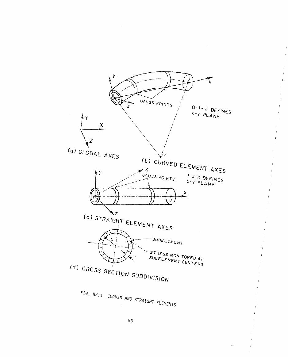
x
0- 1- J DEFINESX-y PLANE
1- J- K DEFINESX-y PLANE
STRESS MON/iORED AiSUBElEMENY C£N'rERS
-
/I
/1 /
\ /\\ /
_~x \\ /
\", /"'lo
(bl CURVED ELEMENT AXES
l
(c I STRAIGHT ELEMENT AXES
I
(d I CROSS SECTION SUBDIVISION
(0) GLOBAL AXES
FIG. 82.1 CURVED AND STRAIGHT ELEMENTS
53
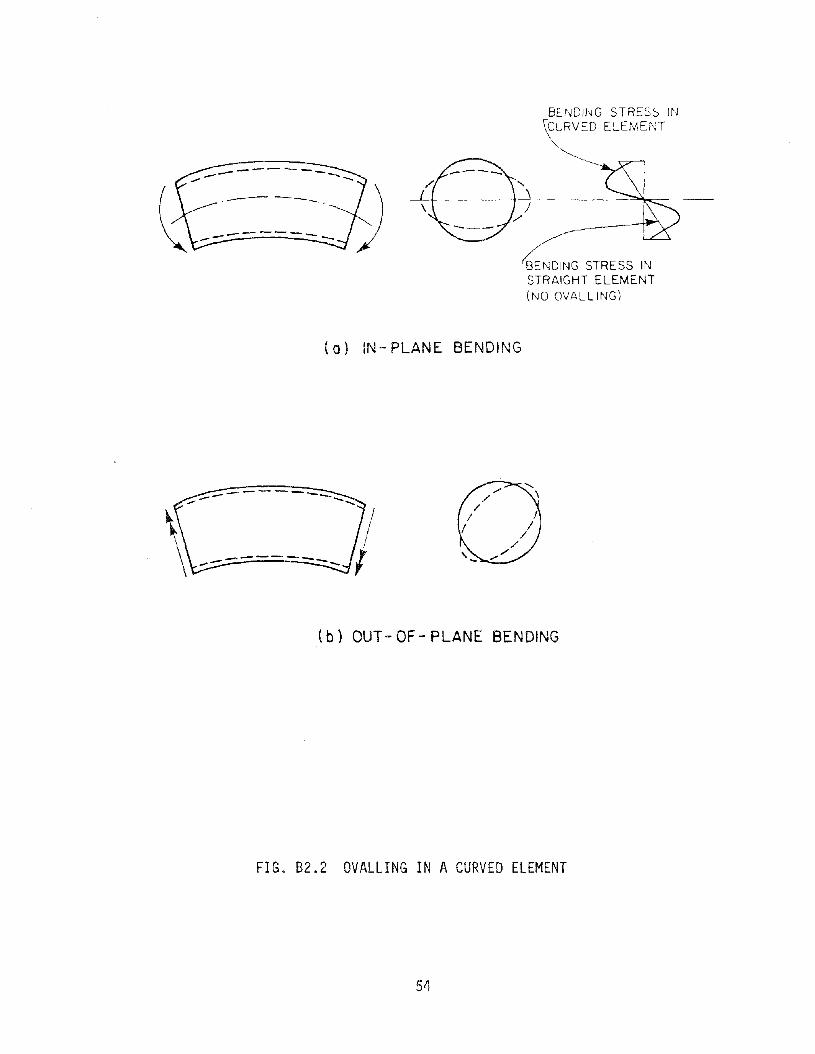
---------...---
BeNDING STRES~ IN\CURVED ELEMENT\
"'-....-...~
)./
~'NSTRAIGHT ELEMENT(NO OVALL ING)
(0) IN-PLANE BENDING
(b) OUT-OF - PLANE BENDING
FIG. 82.2 OVALLING IN A CURVED ELEMENT
54
ySLICES AT INTEGRATION POINTS
,///
__"-?~-----------~~---1I~----+-X
SU8-ELEMENTi
Tr
j jo
FIG. 83.1 CURVED PIPE ELEMENT
55
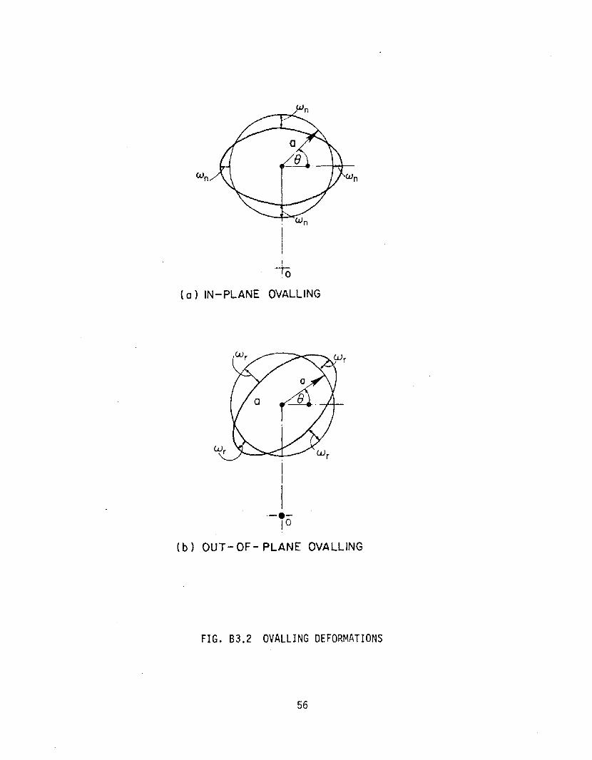
-+0(a) IN-PLANE OVALLING
.-.1°
(b) OUT-OF - PLANE OVALLING
FIG. 83.2 OVALLING DEFORMATIONS
56
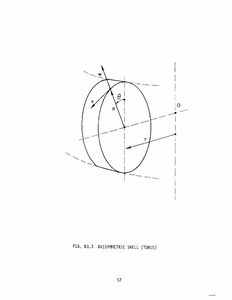
IIII1°
----1----1
FIG. 83.3 AXISYMMETRIC SHELL (TORUS)
57
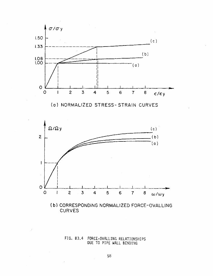
CJ/CJy
€/Ey
( c )
8
( b)
( a)
765432
--------------=--------
O"---_..L.-_...L-_...L..-..-.._...I...U-_-'---_-L-._...J--_...J-- ~
o
1.50
1.33
1.081.00
(0) NORMALIZED STRESS- STRAIN CURVES
8 wlwy76543
( c )
~-----
:;:;;;G===::::::::=========(b )~ (0)
2o ..L.-_...L..-_+-._-'----'---...J----'-----'---_~...
o
2
(b) CORRESPONDING NORMALIZED FORCE-OVALLINGCURVES
FIG. 83.4 FORCE-OVALLING RELATIONSHIPSDUE TO PIPE WALL BENDING
58
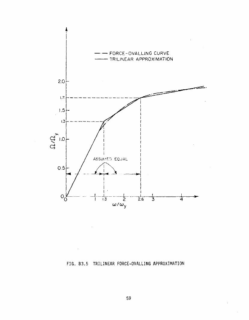
-'- FORCE-OVALLlNG CURVE-- TRILINEAR APPROXIMATION
2.0--.-- .
.~.~.1.71 ----------------
II
1.5 - III
1.3 III
>- I~ 1.0 I........ I~ I
II
ASSUtIE~ EQJAL I
-illI
0.5 I~I
I II II II II I
00 -----_.- _---'___-L.-__ ____i __ __. I I I ...I 1.3 2 2.6 3 4
W/W y
FIG. 83.5 TRILINEAR FORCE-OVALLING APPROXIMATION
59
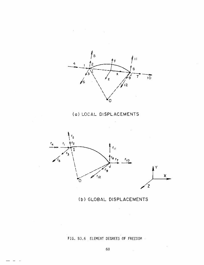
(0) LOCAL DISPLACEMENTS
y
x
(b) GLOBAL DISPLACEMENTS
FIG. 83.6 ELEMENT DEGREES OF FRE~DOM
60
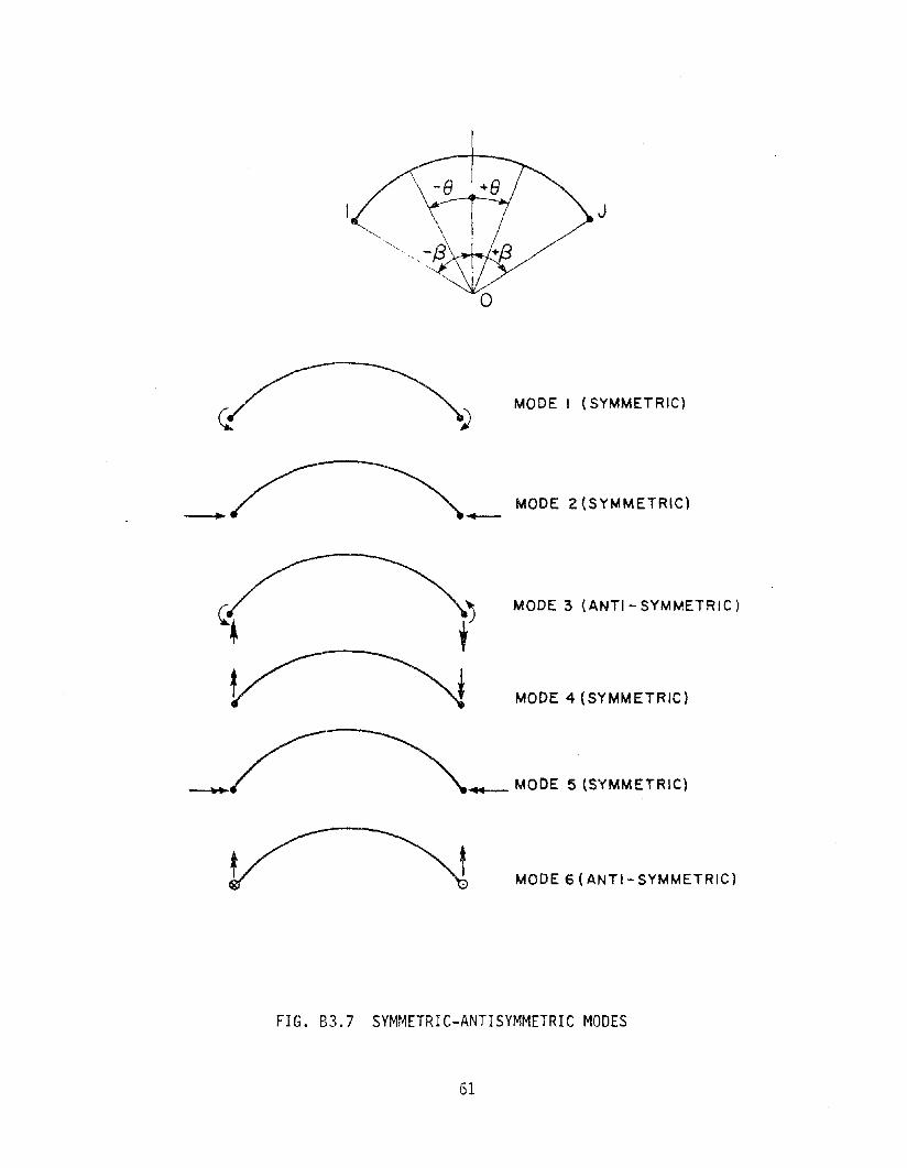
J
MODE I (SYMMETRIC)
MODE 2 (SYMMETRIC)-MODE 3 (ANTI-SYMMETRIC)
MODE 4 (SYMMETRIC)
_ MODE 5 (SYMMETRIC)
MODE 6 (ANT 1- SYMMETRIC)
FIG. B3.7 SYMMETRIC-ANTISYMMETRIC MODES
61
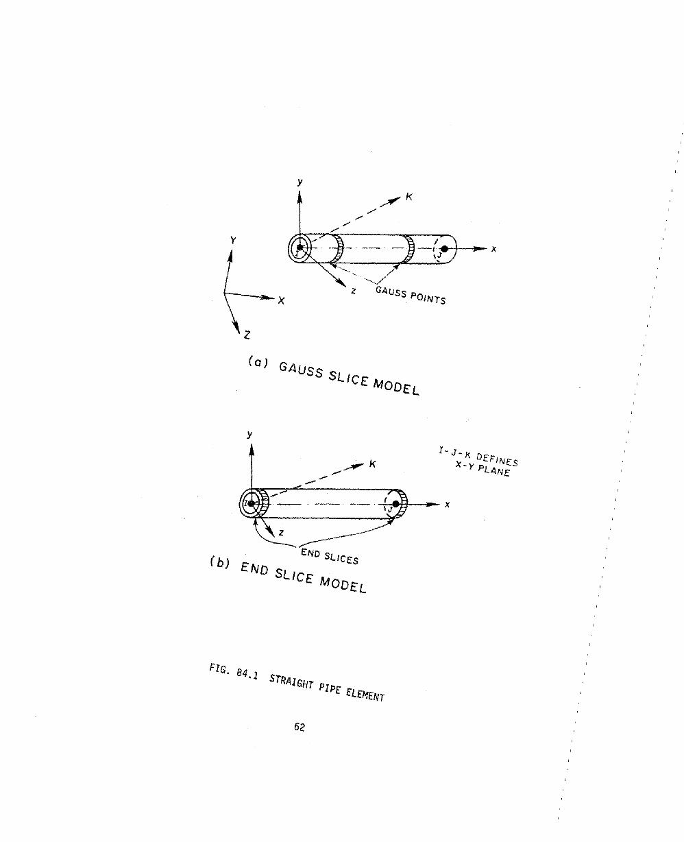
y
t-_-".,_ x
z
y
1- J - k: DEFINESX-y PL4N£
z
----.. END SLICES
(b) fND SliCf MODfL
FIG. 84.1 STRAIGHT PIPE ELEMENT
62
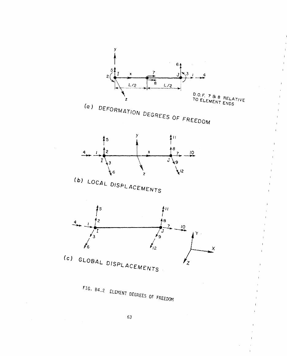
\
Z
x
L/2 ;l/2 -.j
D.O,F. 788 RELATIVETO ELEMENT ENDS
z
y 11/
t ~8 10
\~ -~~--+~--J 9
\12
(b) LOCA L DISPL ACE:ME:NTS
t'f 5
f8 7 104 J tI22------~1c79.J--.. y--.. -'·r
~ I.J' 1216
(e) GLOBAL DISPLACE:ME:NTS
FIG. 84.2 ELEMENT DEGREES OF FREEDOM
63
x
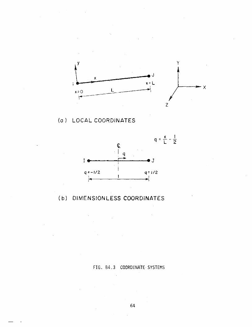
x Iq=--L 2
xx=L
)(=~O ~L__--""'\
\z
(a) LOCAL COORDINATES
~
I q
I ".---~r--""". J
y
J---.....-X
q =-1/2
I.q:: 1/2
~I
(b) DIMENSIONLESS COORDINATES
FIG. B4.3 COORDINATE SYSTEMS
64

C. MULTI·SLICE TUBE ELEMENT
This section describes the theory of the "multi-slice" tube element. The basic features of
the element are described in Chapters Cl and C2. Details of the theory and computational pro
cedure are described in Chapter C3. Chapter C4 contains references, and Chapter CS describes
the input data required for the ANSR-III computer code.
65

C1. INTRODUCTION
CI.I CONCEPT
For finite element analysis of beam-columns, the use of a cubic polynomial shape func
tion implies a linear variation of curvature along the element length. This is correct for a uni
form elastic beam. If the beam becomes inelastic, however, the assumption of linear curvature
variation is no longer correct.
Linear curvature variation within a single element may be reasonable if a complete beam
is subdivided into short elements. However, this is usually not desirable because it increases
the numbers of nodes and elements which must be specified. A compromise is to divide a
complete beam into short subelements and treat the beam as a substructure. This also intro
duces complications, however, one of which is that unbalanced forces will generally be associ
ated with the internal degrees of freedom of the substructure. The need to eliminate these
unbalances adds to the complexity of the analysis.
An alternative approach is to treat a complete beam as a single element and to vary the
shape function as the state of the element changes. Pecknold et al [el ] have used this
approach for reinforced concrete columns, varying the shape function according to predeter
mined rules as the element yields. Their procedure is applicable, however, only for special
cases in which the deformation modes of the element are known fairly accurately in advance.
For the general case it is not possible to establish predetermined rules for variation of the shape
function.
A new procedure has been explored for the "multi-slice" element described herein. With
this procedure, it is not necessary to establish predetermined rules for varying the shape func
tion. Instead, the procedure automatically determines appropriate functions as the analysis
progresses and the state of the element changes.
Preceding page blank67
Cl.2 ELEMENT FEATURES
The basic features of the multi-slice element are as follows. A more detailed qualitative
description is presented in Chapter C2. The theory is presented in Chapter C3.
(}) The element must be straight but may be arbitrarily oriented in space.
(2) Only small element deformations are considered (j.e. the element is assumed to remain
essentially straight>. However, large rigid body motions are permitted.
(3) The element behavior is monitored at a number of slices. one at each end and up to seven
within the element length. The internal slice locations must be specified by the analyst.
These locations must be selected so that spread of plasticity along the element length is
modeled accurately.
(4) Only a pipe cross section is currently permitted. The cross section is subdivided into a
number of subelements (fibers) at each slice. The inelastic behavior at each subelement
is monitored using the Mroz material theory.
68
C2. ELEMENT PROPERTIES
C2.t ELEMENT GEOMETRY
The element geometry and coordinate axes are shown in Fig. C2.l Each element connects
two nodes, each with three translational and three rotational degrees of freedom. The element
does not have any internal degrees of freedom (that is, the theory is not based on substructur
ing concepts).
C2.2 SLICE LOCATIONS
C2.2.1 General
Yielding of the element is monitored at up to 9 slices along the element length, one slice
at each end and up to 7 internal slices. The number of internal slices and their locations must
be specified by the analyst.
Inelastic behavior of a complete element is modeled by monitoring the inelastic behavior
of each slice and assuming linear variation of the inelastic properties between slices (the details
are presented in Chapter C3). The slices must be located in such a way that this linear varia
tion provides a close approximation of the true properties.
C2.2.2 Antisymmetrical Bending
Consider, as an example, an element subjected to equal and opposite end rotations (and
hence end moments), as shown in Fig. C22a. For a rotation value below that causing first
yield, the variations of both bending moment and curvature along the element are linear (Fig.
CZ.2b). The governing inelastic property in this example is the EI value, relating moment to
curvature, which for loading below yield is constant along the element length. Hence, the exact
result can be obtained with only two slices (one at each end), and internal slices are not
needed.
If the element end rotations exceed the yield values, the moment variation along the
length is still linear (because it is governed by equilibrium), but the curvature variation
69
becomes nonlinear (Fig. C2.2c). In this case, if only two slices are assumed, the curvature
variation in the mathematical model is still linear, and the relationship between the actual and
calculated curvatures would be as indicated in Fig. C2.2 d. The maximum curvature would thus
be grossly underestimated.
If, however, four slices are assumed, the curvature variation can be multilinear, for exam
ple, as shown in Fig. C2.2e. A much better approximation of the true curvature variation can
thus be obtained, and the maximum curvature can be predicted more accurately. It may be
noted that the theory actually assumes a linear variation of slice flexibility, represented in this
case by the value lIEI. When this is combined with the linear moment variation, a quadratic
curvature variation can result. This permits a closer approximation of the true curvature than
the multilinear variation shown in Fig. C2.2e.
As the number of slices is increased, the element becomes progressively more accurate.
This is the case, however, only if the additional slices are placed in the part of the element
which yields. Consider the same antisymmetric loading, and assume an elastic-perfectly-plastic
material. For this material, the bending shape factor for a pipe cross section is 1.28. Hence,
the maximum end moment is 1.28 My, where My :0=: moment at first yield, and the maximum
extent of yield in the element is as shown in Fig. C2.3a. In this case, the best results would be
obtained by placing a slice at each end, a slice at the end of each region of potential yield, and
additional slices within the regions of potential yield (Fig. C2.3b). It must be noted, however,
that for materials which are not elastic-perfectly-plastic, the regions of potential yield will be
longer. The situation is also more complex if the bending moment variation is not known, as
considered in the following section.
C2.2.3 Other Bending Moment Variations
Antisymmetrical (or essentially antisymmetricaJ) moment loads, as considered in the
preceding section, are commonly imposed on the members of flexural frames. If it is known in
advance that the element loading will be of antisymmetrical type, slice locations can be selected
as indicated in the preceding section. In general, however, the bending moment variation will
70

not be known in advance. In addition, (l) the moment variation may change progressively; (2)
loading, unloading, and reloading will occur for dynamic or cyclic static loading; and (3) an ele
ment will generally not be subjected to simple uniaxial bending, but to biaxial bending com
bined with axial force, possibly with substantial torsional moments also present. Because of
these factors, the variations of curvature (and other slice deformations) along the element
length may change greatly as a structure is loaded. The problem is more serious if a single ele
ment is used to model a long structural member, and less serious if long members are subdi
vided into several short elements.
At the time of writing, very little experience has been obtained with the multi-slice ele
ment, and resources are not sufficient to perform extensive studies. Hence, no recommenda
tions can be made on the number of slices required for specific cases, nor on their locations.
The examples in Section 0 can provide some guidance.
C2.3 SLICE MODELING
For each slice, the pipe cross section is divided into a number of subelements (typically
12), as shown in Fig. C2.1. The pipe wall at each subelement is assumed to be subjected to
hoop stress (due to pressure), axial stress (due to pressure, bending moment and axial force),
and shear stress (due to torsional moment). The inelastic behavior at the center of each
subelement is monitored using the Mroz material theory. OvaIling of cross sections is not con
sidered.
C2.4 COMPUTATIONAL PROCEDURE
C2.4.1 Shape Function
The computational procedure is described in detail in Chapter C3. The procedure is
essentially as follows.
At any time, the states of stress and strain at all subelements at all slices are known. A
tangent flexibility matrix (4 x 4) is constructed for each slice. For all other cross sections, the
71
flexibility is assumed to vary linearly between the flexibilities of the two adjacent slices. From
the slice flexibilities, a flexibility matrix for the element as a whole is formed (by closed form
integration). From this flexibility matrix, a shape function is constructed, which relates the
deformations at the slices to the displacements of the nodes at the element ends. This shape
function can be used to construct the element tangent stiffness matrix (which turns out, not
surprisingly, to be the inverse of the element flexibility matrix). More importantly, the shape
function is used to determine slice deformation increments in the state determination phase.
C2.4.2 Overshoot and Unloading Tolerances
Each time a cross section subelement yields or unloads, the element flexibility changes.
Hence, the element shape function also changes. For an exact result, the bending moments
must vary linearly along the element, and the axial force and torsional moment must be con
stant. An exact result will be obtained in the state determination phase only if the shape func
tion is recalculated each time a change occurs in the properties of a cross section subelement.
To avoid the computational cost associated with recalculating the shape function each time
a subelement changes its state, some yield overshoot is allowed at the subelement level. The
amount of overshoot is specified by the analyst (typically 2%-100/0 of the material yield
strength). The shape function is recalculated only when the stress in any subelement
overshoots the yield value by the specified overshoot. Several subelements may then have
changed state, and the number of shape function recalculations is reduced.
A similar stress tolerance is used for sUbelement unloading. In addition, it is possible for
the stress at a subelement to move around the Mroz yield surface so that the direction of plastic
flow changes. Such a change in direction changes the tangent stress-strain relationship, and
hence, also the slice and element stUfnesses. To avoid recalculation of the shape function each
time a flow direction changes slightly, the analyst is required to specify an angle tolerance (typi
cally about 0.1 radians). The shape function is recalculated only if the flow direction at any
subelement changes by more than this tolerance.
72
C3. THEORY
C3.1 PROCEDURE AND ASSUMPTIONS
The stiffness and state determination calculations for the element are based essentially on
beam theory. The theory is presented herein for a pipe element with a thin-walled circular
cross section. The theory can be modified for other cross section shapes.
The element is modeled as shown in Fig. C3.1. One beam slice is located at each element
end, and a maximum of seven additional slices may be specified at arbitrary locations along the
element length. Each slice is divided into a number of cross section subelements. The subele
ment stiffnesses are constructed first, allowing for elasto-plastic behavior of the pipe steel. The
slice stiffnesses are constructed from the subelement stiffnesses by summation. The slice flexi
bilities are obtained by inverting the slice stiffnesses, and a complete element flexibility is con
structed from the slice flexibilities by closed-form integration. The element stiffness is then
obtained by inverting the element flexibility.
The deformations at any slice consist of six beam-type deformations, namely axial defor
mation, torsional twist, major plane and minor plane curvatures, and major plane and minor
plane flexural shear deformations. The major plane is assumed to be the local xy plane.
Cross-section warping is not considered in the theory presented herein.
The complete element has six nodal degrees of freedom at each end, which provide six
rigid body modes plus six element deformations. The slice deformations are related to the ele
ment deformations by shape functions, which are progressively updated as the element yields.
Each subelement is assumed to be in a state of plane stress, with axial, hoop, and shear
stresses. The effects of axial deformation and curvature on the axial strains are determined
assuming a plane, circular cross section. The shear strain is assumed to be affected by torsional
twist only. Flexural shear effects are assumed to be negligible at the subelement level and are
ignored (they are introduced at the slice level). The subelement shear strains due to twist are
determined assuming plane, circular cross sections.
73
Hoop strains are not determined from strain-displacement relationships. Rather, the hoop
stresses are governed by the equilibrium relationship between internal pressure and hoop stress.
The hoop strain in any subelement thus becomes an internal degree of freedom for the subele-
ment and is condensed out before the slice stiffness is calculated.
C3.2 SLICE STIFFNESS
C3.2.t Deformations and Actions
The slice deformation vector, l's. is given by:
(C3. J)
in which B -= axial strain at pipe axis; '"z ... bending curvature about element z axis; '" y =
bending curvature about yaxis; rJ> .. rate of torsional twist; 'Y.xy .. flexural shear deformation in
x-y plane; and 'Y xz ... flexural shear deformation in x-z plane.
The corresponding slice action vector is ~s, where
(C3.2)
in which F == axial force; Mz and My .. bending moments; T .. torsional moment; and V.x)
and Vxx .. flexural shear forces.
C3.2.2 Strain-Deformation Relationships for Slice
Consider slice subelement i, located at angle (J i (Fig. C2.l(b». The subelement mem-
brane strains, E Qi and 'Y it are related to the slice deformations by:
in which
dE r - < dE . d'Y >_I _QI I
(C3.3)
(C3.4)
!Oi .. axial strain in subelement i; 'Y i .. torsional shear strain; l's is defined by Eqn. C3.1; and
B 11 asin8 i -aeos9 i 0 0 01_i - 0 0 0 a 0 0 (C3.5)
This transformation assumes that plane sections remain plane and circular. It is also implied
74
(C3.6)
that the pipe thickness is small compared to the pipe diameter.
Note that the slice shear deformations, 'Y xy and 'Y XI' are assumed not to influence the
subelement strains. The effects of these deformations are considered separately.
C3.2.3 Stress-Strain Relationships for Slice S3llbeJement
Each subelement is assumed to be in a state of membrane stress and strain (plane stress).
The hoop stress is controlled by the internal pressure, according to the well-known equation
p (a-O.5t) Po'fTh- ---
t t
in which P = internal pressure; a = radius to pipe wall mid-thickness; t == wall thickness~ and
0' - a-0.5t.
The Mroz plasticity theory is used to model subelement yield. The details of the pro-
cedures used to implement this theory have been described in detail by Mosaddad [e 2J and
are not repeated here. For any given state of subelement i, an elasto-plastic stress-strain rela-
tionship is determined as
in which
dfT T - < dfT ai dT; dfT hi >
d!.I - < dE ai dy; dE hi >
(C3.7)
(C3.8)
(C3.9)
where fT hi = hoop stress in subelement i (the same in all subelements); E hi = hoop strain in
subelement i; and !2; = 3 x 3 elasto-plastic constitutive matrix. From Eqns. C3.7 and C3.6 it
follows that
(C.lIO)
in which dP is known. Hence,.Q; can be reduced, by static condensation, to a 2 x 2 matrix,
/2,;, in terms of axial and shear stresses only. If dP = 0, the result can be written as:
lDJ! dE Oil _ !dfT a'i-" dy i d'T;
75
(C3.II)
If dP is not zero, an initial stress effect must be included.
C3.2.4 Stiffness Matrix
The transformation matrix .u (Eqn. C3.5) considers the effects of axial deformation,
bending, and torsion. A tangent stiffness matrix for the slice, !s' which considers only these
effects, is thus given by:
(C3.12)
in which N .... number of slice subelements around pipe circumference.
The matrix !s has zero rows and columns corresponding to the shear deformations y xy
and y xz, because the transformation .u does not consider flexural shear effects. It is assumed
that the flexural shear stiffness is not affected by yielding of the element, and hence, that the
elastic shear stiffness can be used. For an effective shear area equal to one-half of the cross
section area, the shear stiffnesses are defined by:
dVxy - G'lrot· dy xy - k y ' dy xy
and
<C3.13a)
<C3.13b)
in which G .... elastic shear modulus. The slice stiffness coefficients ks(S,S) and ks<6,6) are set
equal to kyo
C3.3 SLICE FLEXIBILITY
The slice flexibility, is' is obtained by inverting the slice stiffness. That is,
(C3.14)
In the computer coding, the 4 x 4 slice stiffness without the shear stiffness is first inverted, and
the flexibility coefficients Is(5,5) and Is(6,6) are set equal to 1/ kyo
76
C3.4 ELEMENT STIFFNESS
C3.4.1 Deformations and Actions
The element deformations and displacements are shown in Fig. C3.2. The element
degrees of freedom, after deletion of the six rigid body modes, are defined by the vector .l'm,
where:
.!! .. < Ux 9zi Bzj Bx Byi Byj > (C3.IS)
where Ux .. axial extension; 9zi ... z-axis rotation at element end i; () zj = z-axis rotation at end
j~ Bx ... torsional twist; 9yi ... y-axis rotation at end i~ and 9yj = y-axis rotation at end j.
The corresponding element action vector is §m, where:
(C3.I6)
C3.4.2 Shape Function Calculation
For finite element analysis of straight beams, it is common to use a cubic Hermitian poly
nomial shape function. This permits a linear curvature variation and is exact for a uniform
elastic beam loaded only at its ends. If the beam becomes inelastic, however, the assumption
of linear curvature variation is no longer correct and equilibrium within the element is violated.
This can lead to serious errors. For the multi-slice element, however, it is possible to calculate,
for any state of the element, an "exact" shape function. This shape function is calculated by the
computer program and is progressively updated as the state of the element changes.
A multi-slice shape function can be calculated using either a stiffness or a flexibility
approach. Both approaches have been explored and that based on flexibility has been found to
be superior. For completeness, the steps for both approaches are considered in the following
sections.
C3.4.3 Stiffness Approach
The stiffness approach is based on substructuring theory, in which a complete element is
regarded as a substructure divided at the internal slices into a number of substructure elements
77

(Fig. C3.3 ). The steps in the computation are as follows.
(}) For each slice, form the current tangent stiffness, 55' using Eqn. C3.12.
(2) Place "external" nodes at the two end slices and an "internal" node at each internal slice,
dividing the substructure into several elements. Each node has three translational and
three rotational degrees of freedom. The properties of each substructure element are
determined by the properties of the two slices which the element joins.
(3) For each substructure element assume a cubic shape function, and assume that the
stiffness varies linearly along the element length (j.e., interpolate between the slice
stiffnesses, 55' for the slices which the element joins). With this assumption a stiffness
matrix can be calculated in closed form for each substructure element.
(4) Assemble the element stiffnesses to obtain a complete substructure stiffness, in terms of 6
displacements at each internal node and a total of 6 displacements at the two external
nodes. The external node displacements are conveniently chosen as those shown in Fig.
C3.3.
(5) Select one of the 6 external node displacements. Impose a unit value of this displace
ment, with the remaining 5 external displacements constrained to be zero and all internal
displacements unrestrained. Solve for the internal displacements.
(6) Using the displacements from Step (5) and the cubic shape functions for the substructure
elements, calculate the slice deformations at the two ends of each element. Two slice
deformation vectors will be calculated for each internal slice, and these will not necessarily
be equal. Average the two vectors to obtain the slice deformations.
(7) The slice deformations from Step (6) define one column of the shape function for the
complete element (i.e. the deformations at all slices for a unit value of one external dis
placement). Repeat Steps (5) and (6) for each external displacement in turn to obtain a
complete displacement transformation matrix.
78

C3.4.4 Weaknesses of Stiffness Approach
The procedure described in the preceding section has been explored and found to have a
number of weaknesses when compared with the flexibility approach. These weaknesses are as
follows.
(I) The calculated slice deformations are discontinuous at the internal nodes, and average
values are used to obtain the shape functions. This averaging is not necessary in the flexi
bility approach.
(2) The calculated element stiffness is only approximate, whereas that obtained by the flexi
bility approach is "exact".
(3) The computational cost is higher than for the flexibility approach.
C3.4.5 Flexibility Approach
The flexibility approach also considers a complete element as a substructure consisting of
a number of substructure elements. However, the substructure flexibility properties are deter
mined, rather than its stiffness properties. The flexibility properties are then used to determine
both the stiffness matrix for the complete element and the element shape function. The pro
cedure is as follows.
(1) For each slice, form the current tangent flexibility, is, using Eqn. C3.14.
(2) Select the displacements shown in Fig. C3.4 as the substructure deformations, and the
corresponding forces as the substructure actions. The substructure is thus statically deter
minate.
(3) From equilibrium Oinear variation of slice actions along the substructure length), express
the actions at each slice in terms of the substructure end actions. This defines a force
transformation matrix.
(4) Assume that the slice flexibility varies linearly between each pair of slices. Hence, using
the force transformation from Step (3), determine the substructure flexibility matrix.
79
(5) Obtain the shape function using the substructure flexibility from Step (4), the slice flexi-
bilities from Step (I), and the force transformation from Step 0), The theory is
presented in the next section. Also obtain the substructure (j.e. complete element)
stiffness as the inverse of the substructure flexibility.
C3.4.6 Flexibility Calculation
An element flexibility in terms of the element degrees of freedom after deletion of the six
rigid body modes is first obtained. This flexibility is then used to obtain the shape functions.
The element actions correspond to the six deformations shown in Fig. C3.4. The equili-
brium relationship between the slice actions and the element actions is:
in which ~s and §m are defined by Eqns. (C3.2) and (C3.l6), respectively, and
(C3.17)
b
1 0 0 0o 1-xl L - xl L 0o 0 0 0o 0 0 1o II L II L 0o 0 0 0
o 0o 0
I-xl L -xlLo 0o 0
-IlL -IlL
(C3.I8)
A slice flexibility relationship can be written as:
d~s ... Is §s
in which [s is the inverse of the slice stiffness, !s' developed in Section C3.2.
(C3.19)
Equations C3.17 and C3.19, plus a standard application of the virtual forces principle, lead
to the element flexibility relationship:
in which
d~m - 1m dJm (C3.20)
(C3.21)
After transformation to dimensionless coordinates, q, as shown in Fig. C3.5, Eqn. C3.2I
becomes:
'Ii
1m - t L i J l!llsilli dqi-I -Iii
80
(C3.22)
in which n = number of substructure elements (equal to the number of slices minus one)~ and
L; -= length of element i. The integration in Eqn. C3.22 can be carried out in closed form if it
is assumed that the slice flexibility, is> varies linearly between slices.
C3.4.7 Shape Function
The deformation increments at any slice, d~s' can be obtained in terms of the element
deformations (Fig. C3.4 ), as follows.
From Eqns. C3.17 and C3.19:
Hence, from Eqn. C3.20:
d~s - is.!! ~m (C3.23)
(C3.24)
The shape functions relating increments of slice deformation to increments of element defor-
mation can thus be expressed as:
(C3.25)
C3.4.8 Element Stiffness
From the slice stiffness relationship of Eqn. C3.12, the transformation relating slice defor-
mations and element deformations (Eqn. C3.25) and standard application of the virtual dis-
placements principle, the complete element stiffness can be obtained as:
(C3.26)
Hence, substitute E from Eqn. C3.25 into Eqn. C3.26, and note that is -= lss-I, to get:
L
K f [;;I!?Tislssis!?i;,1 dxo
i -I JbTL b dx '1- 1m _ s_ m
o(C3.27)
That is, the element stiffness matrix obtained using the shape function is the same as that
obtained by inverting the element flexibility. Computationally, the element stiffness is obtained
81
from Eqn. C3.27 and the shape function is thus used only in the state determination phase.
The stiffness K is in terms of element deformations only. It is expanded to include the ele
ment rigid body displacements, and then transformed to the 12 x 12 global stiffness. The
transformations are well known and are not repeated here.
C3.S STATE DETERMINATION
C3.S.l Basic PrOtedure
The shape function, fl, defined by Eqn. C3.25 is exact for an infinitesimally small dis-
placement increment. For such an increment, the slice deformation increment is obtained
using the shape function as:
Hence, the slice action increment is:
dJs .. lis dl's
!isE d1m
(C3.28)
(C3.29)
From Eqns. C3.25 and Cl27, this is the same as:
~s .. !isis! K d.!m
.. pK d.!m (C3.30)
Alternatively, the slice action increment can be obtained directly from the equilibrium relation-
ship as:
d§s .p d§m
.. .p K dlm (C3.31)
These two approaches thus given the same result, which reflects the fact that the shape function
is "exact" for infinitesimal element deformations. In an actual state determination, however,
the element deformation wiU be finite. This introduces two complications, one associated with
the material calculations, and a more important one associated with change in the shape rune-
tion. These complications are considered in the following sections.
82
C3.S.2 Linearity in Mroz Material Calculations
In the state determination calculation for the Mroz material, the stresses are calculated
assuming linear behavior. They are then scaled so that the stress point lies exactly on the yield
surface. This means that the calculated hoop stress in any slice subelement may not exactly
satisfy £qn. C3.6. If this error is not corrected, it may accumulate over a number of load incre
ments and introduce significant inaccuracy in the solution.
The error is corrected by determining, for each slice subelement, the internal pressure
corresponding to the calculated hoop stress. The difference between this pressure and the
actual pressure is then a "pressure error." At each iteration, this pressure error is added to dP in
£qn. C3.10 and treated as an initial stress effect.
C3.S.3 Linearity in Use of Shape Function
If the shape function is assumed not to change for a finite deformation increment of the
element, the slice deformation increments are given by Eqn. C3.28. The strains in the slice,
and hence the subelement stresses and slice actions, then follow. However, if the slice defor
mation increments are sufficiently large that additional yielding (or unloading) occurs, the shape
function will change, and hence the calculated slice actions will not satisfy the equilibrium
requirement (£qn. C3.l7). If equilibrium errors develop and are not corrected, they can accu
mulate over a number of load increments and reach a significant magnitude.
Internal equilibrium errors may be avoided by either a "prevention" or a "correction"
approach. In the prevention approach, the state determination calculation is divided into small
steps so that no significant equilibrium errors develop. In the correction approach, large steps
are allowed and equilibrium errors are permitted to develop. These errors are then eliminated
by applying corrections in subsequent state determinations. Both approaches have been
explored, and that based on prevention has been found to be more stable. For completeness
the procedures for both approaches are described in the following sections.
83
C3.S.4 Prevention Approach
The prevention approach seeks to prevent significant internal equilibrium errors from
developing by adjusting the shape function, 0, each time a significant change (an "event")
oceurs in the element state. An event occurs if significant yielding or unloading occurs in any
slice subelement. The definition of "significant" is controlled by means of an overshoot toler-
anee, which allows subelements to go somewhat beyond new yield or unloading before an event
is detected.
When an increment of global displacement, 41, has been determined, the state determi-
nation proceeds as follows.
(1 ) Calculate the element deformation increment:
(C3.32)
in which Er is a well known displacement transformation matrix.
(2) Calculate the slice deformation increments:
(C3.33)
using the current shape function, E.
(3) Calculate the subelement axial and shear strain increments from Eqn. C3.3.
(4) Calculate the subelement hoop strain increments from:
<C3.34)
in which Dlj == term in the constitutive matrix, ]2, and the hoop stress error is obtained
from:
no'Ao- h = L=- - 0- h
• t(C3.35 )
(5) Calculate, for each subelement, an event factor, allowing for overshoot of yield or unload-
ing.
(6) Use the minimum event factor from Step (5) to scale the subelement strain and element
deformation increments. Using the scaled strain increments. obtain the subelement stress
84
(7) If no event has occurred, the state determination is complete. If an event has occurred,
recalculate the shape function.
(8) Apply the remainder of the element deformation increment, and repeat from Step (2).
When the final subelement stresses have been calculated, the slice actions are obtained by sum-
mation over the slice cross sections. If the slice actions were to satisfy equilibrium exactly (j.e.
linear variation along the element length), the element end actions would be simply the actions
on the two end slices. In fact, the slice actions will not exactly satisfy internal element equili-
brium, and it is advisable to obtain the element actions using the virtual displacements princi-
pIe.
In applying the virtual displacements principle, the natural approach would be to impose a
virtual displacement defined by the current shape function, £. This is not essential, however.
It is interesting to note that if the slice actions satisfy equilibrium (linear variation), then any
virtual displacement which satisfies compatibility will give the same result (namely that the ele-
ment end actions equal the actions on the end slices). If the slice actions do not exactly satisfy
equilibrium, then the element end actions calculated by the virtual displacements principle will
not be the same for all virtual displacements. However, the differences should be small, and
one virtual displacement is not necessarily better than any other. For the ANSR-III implemen-
tation, the linear elastic shape function, g/, has been used to define the virtual displacement,
and the element end actions are thus obtained as:
<C3.36)
This equation has the advantage that £/ defines a linear variation of deformation along the ele-
ment length, and the integral is easily evaluated in closed form. If the current shape function,
g, is used, the deformations vary quadratically, and evaluation of the integral is more difficult.
The use of £1 is equivalent to assuming that the element is unloaded by an infinitesimal
amount, so that it becomes elastic but the slice actions do not change. The "current" shape
function thus becomes !!/, which is then used to define the virtual displacement.
85

C3.S.S Correction Approach
The correction approach allows large steps to be taken and avoids event calculations.
However, substantial equilibrium errors may result, which must be corrected in subsequent
state determinations. The corrections are made by introducing internal degrees of freedom into
the element to allow the element to adjust its shape internally, and hence, satisfy internal
equilibrium.
One possible approach is to add internal nodes to the element and let the displacements of
these nodes be the internal degrees of freedom. This approach, however, is exactly the same as
substructuring. It requires that the analyst select appropriate internal nodes and substantially
complicates the computational procedure. Hence, this approach was not considered.
An alternative approach is to select one or more generalized internal degrees of freedom
(j.e., not necessarily physical displacements) and to let the shape functions associated with
these degrees of freedom vary during the analysis. This approach is consistent with the variable
shape function concept used for the element end displacements (the external degrees of free-
dom). It has been explored, as follows, for a single internal degree of freedom.
Let the added internal degree of freedom be Va' and let its shape function at any time be
fla. Hence, slice deformation increments are given by:
(C3.37)
If a set of virtual element actions, §m, is applied, the rolJowing virtual work equation must be
satisfied:
~;;; d~m - f §td~s dxL
... §;;; .f }Tfl dx . dl'm + ~;;; .f }TEo dx . dvoL L
From this equation it follows that:
(C3.38)
1 (C3.39)
in which 1 is a unit matrix, and:
86
in which 1 is a unit matrix, and:
in which Q is a null vector.
o (C3.40)
Equation C3.39 is satisfied automatically. The shape function associated with the internal
degree of freedom must satisfy Eqn. C3.40. A convenient choice for flo is t>.!J., which is the
change in !J. when it was last reformed. Because Eqn. C3.39 is satisfied for both !J. (the current
shape function) and !J. - t>.fl (the preceding shape function), it follows that Eqn. C3.40 is
satisfied by flo = t>.!J.. The computational procedure for the state determination is as follows.
(I) Calculate the element deformation increment from Eqn. C3.32.
(2) Calculate the slice deformation increment:
(C3.41 )
in which t>.iso is an initial slice deformation increment obtained from the previous state
determination, as described later in Step (I 0),
(3) Calculate the axial, shear, and hoop strain increments from Eqns. C3.3 and C3.34.
(4) Obtain the subelement stresses by Mroz material state determination.
(5) Reform the shape function, fl, if substantial yielding or unloading has occurred. Hence.
also obtain, t>.!J..
(6) Obtain the slice forces, §.s, by summing the stresses over the cross section.
(7) Calculate the element end actions, §.m, from Eqn. C3.36.
(8) Calculate the equilibrium error at the slices, t>.~e, as:
(C3.42)
(9) Calculate slice force increments associated with a unit increment in the internal degree of
freedom, t>. Vo = 1, as:
(C3.4Jl
87
(0) Obtain the value of a Va which minimizes the slice force errors. That is, select al'a so
that, say, the RMS value of:
a~e - 4~a 4 Va
is a minimum. The slice deformations:
(C3.44)
become initial slice deformations to be taken into account in the next state determination
(Step 2).
A number of analyses were carried out to explore this procedure. The results were
encouraging provided only small element deformation increments were allowed in any load
step. If large deformation increments were allowed, however, the initial slice deformations,
4l'so' tended to dominate the response. There was then a tendency for successive yielding and
unloading to occur within the element, leading to numerical instability. For this reason it was
decided to implement only the "prevention" approach in the ANSR-III element.
88
C04. REFERENCES
Cl. Suharwardy, M.I.H. and D. A. Pecknold, "Inelastic Response of Reinforced ConcreteColumns Subjected to Two-Dimensional Earthquake Motions," Structural Research SeriesNo. 455, Department of Civil Engineering, University of Illinois at Urbana-Champaign,October 1978.
C2. Mosaddad, B., "Computational Models for Cyclic Plasticity, Rate Dependence and Creep,"Ph.D. Thesis, Civil Engineering Department, University of California, Berkeley, June1982.
89

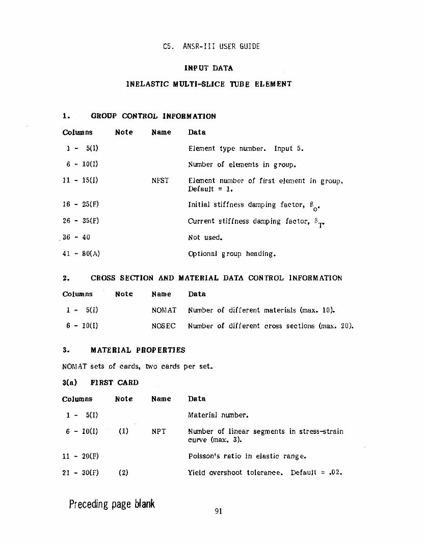
C5. ANSR-III USER GUIDE
INPUT DATA
INELASTIC MULTI-SLICE ruBE ELEMENT
1. GROUP CONTROL INFORMATION
Columns
1 - 5(1)
6 - 10(1)
11 - 15(1)
16 - 25(F)
26 - 35(F)
36 - 40
41 - BO(A)
Note Name
NFST
Data
Element type number. Input 5.
Number of elements in group.
Element number of first element in group.Default = 1.
Initial stiffness damping factor, So.
Current stiffness damping factor, Sr
Not used.
~tional g roup heading.
2. CROSS SECTION AND MATERIAL DATA CONTROL INFORMATION
Columns Note Name Data
1 - 5(I)
6 - 10(1)
NOMAT Number of different materials (max. 10).
NOSEC Number of different cross sections (max. 20).
3. MATERIAL PROPERTIES
NOMAT sets of cards, two cards per set.
3(a) FIRST CARD
Columns
1 - 5(1)
6 - 10(1)
11 - 20(F)
21 - 30(F)
Note
(1)
(2)
Name
NPT
Data
Material number.
Number of linear segments in stress-straincurve (max. 3).
Poisson's ratio in elastic range.
Yield overshoot tolerance. Default = .02.
Preceding page blank91
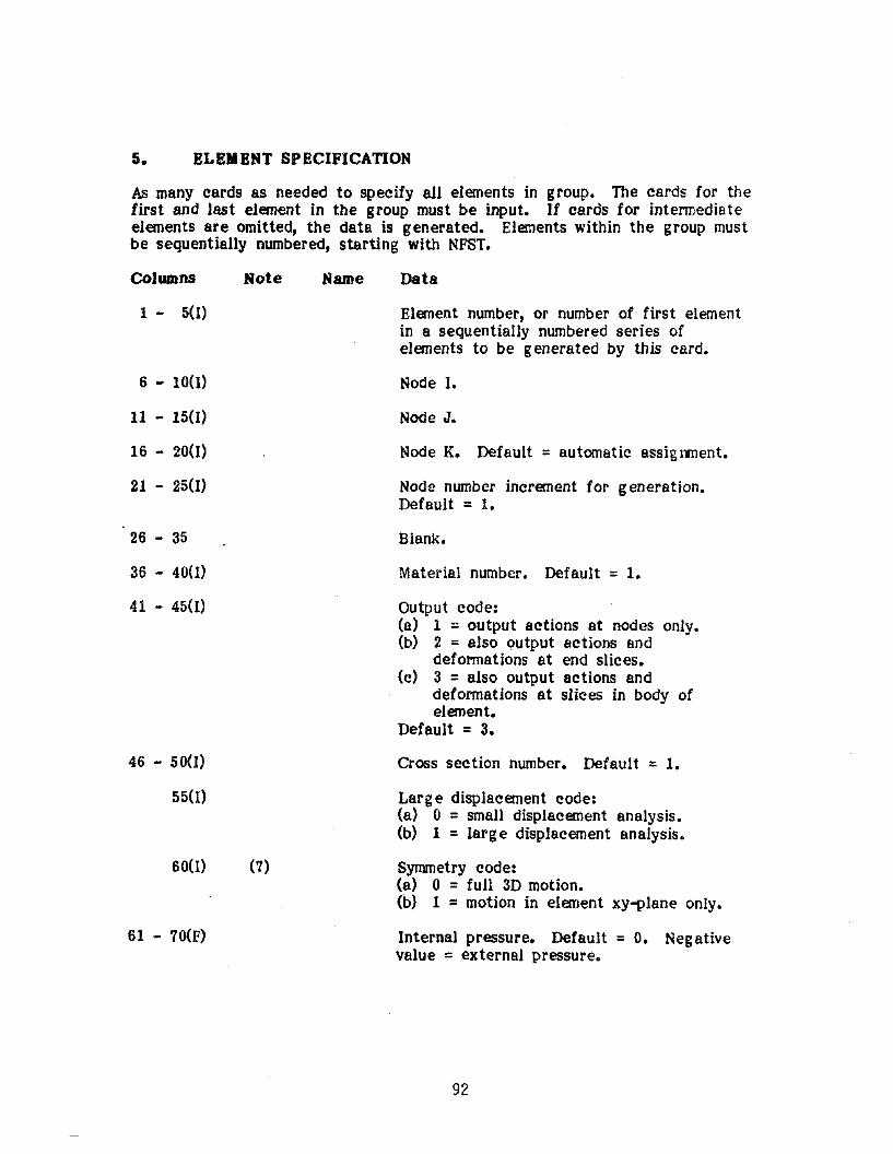
5. ELEMENT SPECIFICATION
As many cards as needed to specify all elements in group. The cards for thefirst and last element in the group must be input. If cards for intermediateelements are omitted, the data is generated. Elements within the group mustbe sequentially numbered, starting with NFST.
Columns
1 - 5(1)
6 - 10(1)
11 - 15(1)
16 - 20(1)
21 - 25(1)
26 - 35
36 - 40(1)
41 - 45(1)
46 - 50(I)
55(I)
60(I)
61 - 70(F)
Note
(7)
Name Data
Element number, or number of first elementin a sequentially numbered series ofelements to be generated by this card.
Node I.
Node J.
Node K. Default =automatic assignment.
Node number increment for generation.Default =1.
Blank.
Material number. Default =1.
Output code:(a) 1 =output actions at nodes only.(b) 2 = also output actions and
deformations at end slices.(c) 3 =also output actions and
deformations at slices in body ofelement.
Default =3.
Cross section number. Default =1.
Larg e displacement code:(a) 0 =small displacement analysis.(b) 1 =large displacement analysis.
Symmetry code:(a) 0 =full 3D motion.(b) 1 =motion in element xy~lane only.
Internal pressure. Default = O. Negativevalue =external pressure.
92
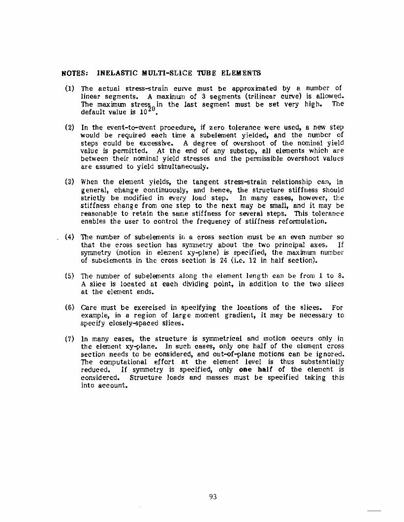
NOTES: INELASTIC MULTI-SLICE TUBE ELEMENTS
(1) The actual stress-strain curve must be approximated by a number oflinear segments. A maximum of 3 segments (trilinear curve) is allowed.The maximwn stres~o in the last segment must be set very high. Thedefault value is 10 •
(2) In the event-to-event procedure, if zero tolerance were used, a new stepwould be required each time a subelernent yielded, and the number ofsteps could be excessive. A degree of overshoot of the nominal yieldvalue is permitted. At the end of any substep, all elements which arebetween their nominal yield stresses and the permissible overshoot valuesare assumed to yield simultaneously.
(3) When the element yields, the tang ent stress-strain relationship can, ingeneral, change continuously, and hence, the structure stiffness shouldstrictly be modified in every load step. In many cases, however, thestiffness chang e from one step to the next may be small, and it may bereasonable to retain the same stiffness for several steps. This toleranceenables the user to control the frequency of stiffness reformulation.
. (4) The number of subelements in a cross section must be an even number sothat the cross section has symmetry about the two principal axes. Ifsymmetry (motion in element xy-plane) is specified, the maximum numberof subelements in the cross section is 24 (i.e. 12 in half section).
(5) The number of subelements along the element length can be from 1 to 8.A slice is located at each dividing point, in addition to the two slicesat the element ends.
(6) care must be exercised in specifying the locations of the slices. Forexample, in a region of large moment gradient, it may be necessary tospecify closely-spaced slices.
(7) In many cases, the structure is symmetrical and motion occurs only inthe element xy-plane. In such cases, only one half of the element crosssection needs to be considered, and out-{)f-plane motions can be ignored.The computational effort at the element level is thus SUbstantiallyreduced. If symmetry is specified, only one half of the element isconsidered. StructUre loads and masses must be specified taking thisinto account.
93

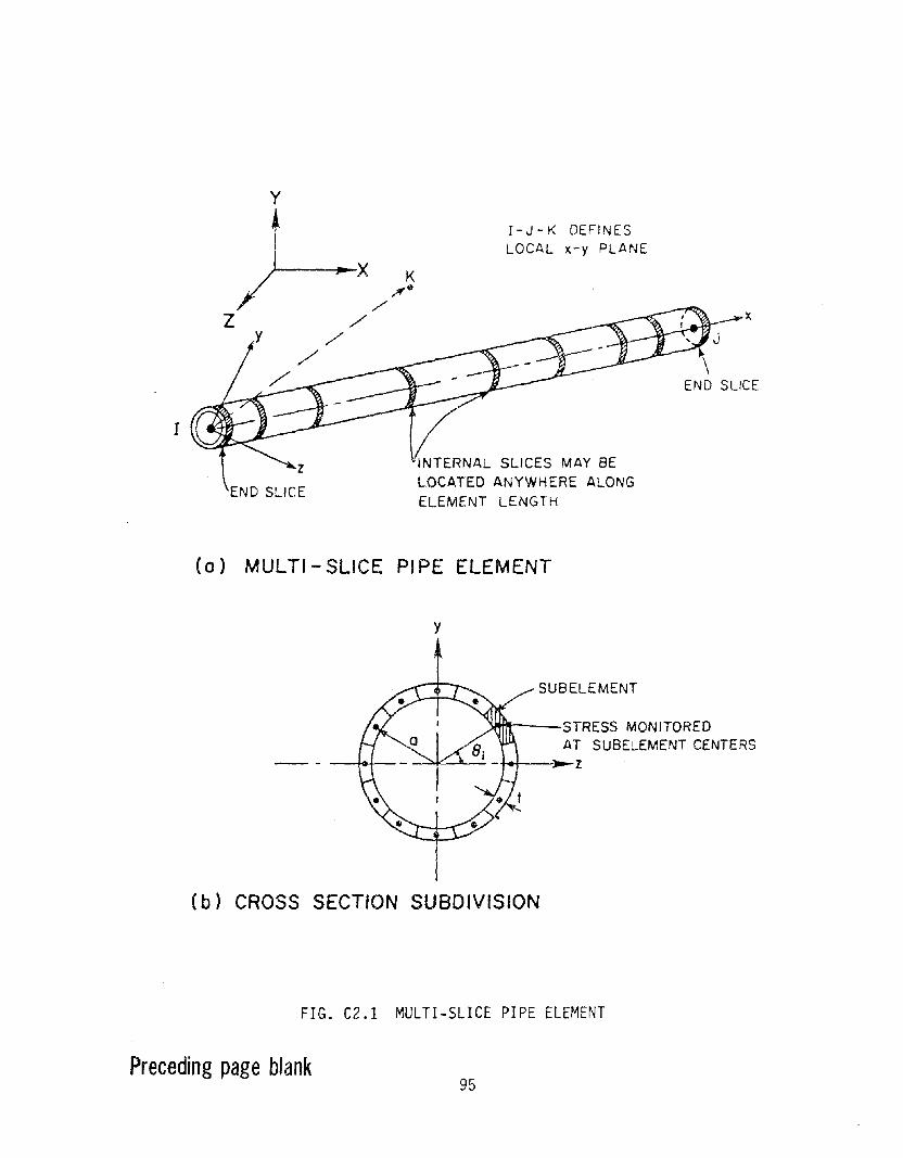
r
y
t)---
x K",,0
./'Z /'
/'/
/
I-J-K DEFINESLOCAL x-y PLANE
INTERNAL SLICES MAY BELOCATED ANYWHERE ALONGELEMENT LENGTH
x
(0) MULTI- SLICE PI PE ELEMENT
y
- - -#+--
SUB ELEMENT
WI*--STRESS MONITOREDAT SUBELEMENT CENTERS
~----z
(b) CROSS SECTION SUBDIVISION
FIG. C2.1 MULTI-SLICE PIPE ELEMENT
Preceding page blank95
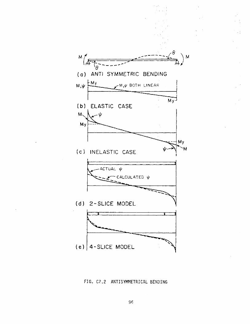
M f ~ ... 2<_-------£8 ) M
(~ -t :.- - ---- ~8 --( a) ANTI SYMMETRIC BENDING
M.o/~BO~ jMy
( b)
M
CASE
INELASTIC CASE
ACTUAL 0/
- -- r- CALCULATED \f!
---
(d) 2 - SLICE MODEL
( e) 4 - SLICE MODEL
FIG. C2.2 ANTISYMMETRICAL BENDING
96
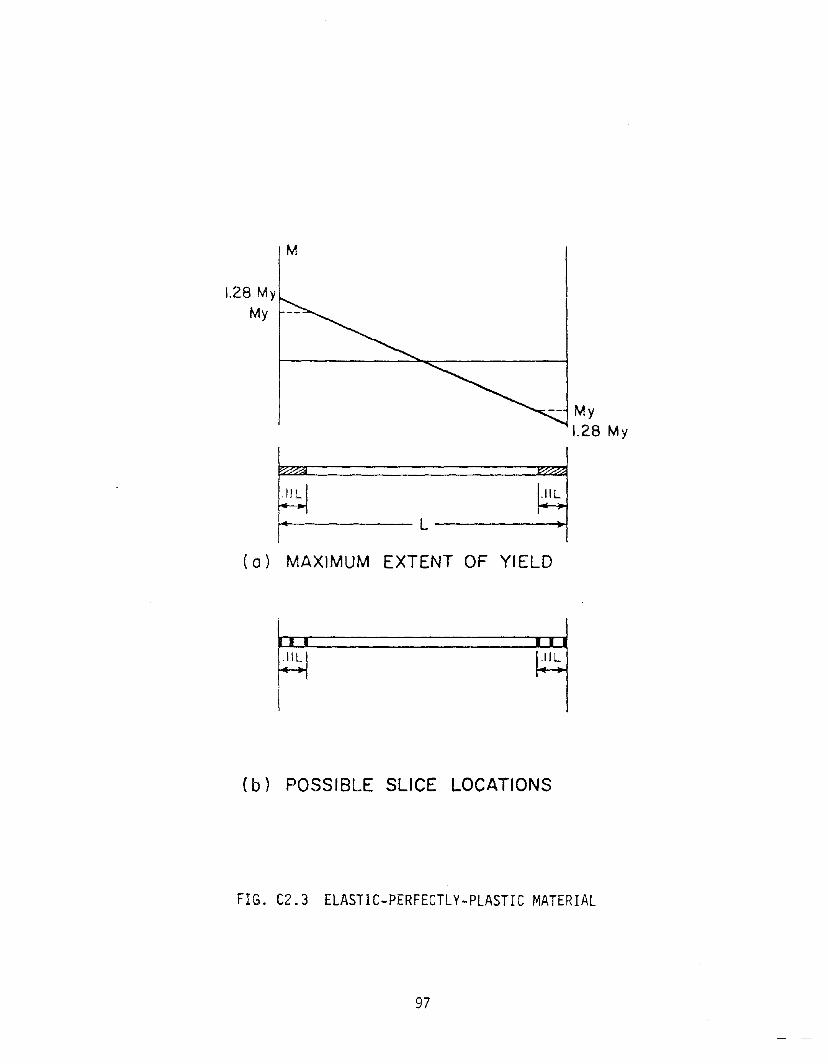
M
1.28 MyMy --
-- My1.28 My
~----- L-----~
(a) MAXIMUM EXTENT OF YIELD
II I I I
.IIL~
(b) POSSIBLE SLICE LOCATIONS
FIG. C2.3 ELASTIC-PERFECTLY-PLASTIC MATERIAL
97
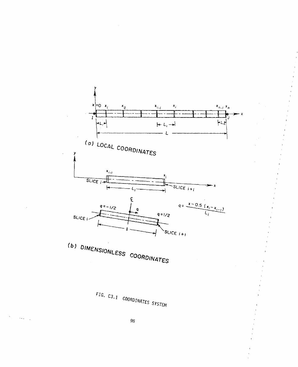
y
SLICE i)(jX~i_I:"- --:-==~ ~_ )(
SLJCEi+/
q....---.....- - ---.1-'__
~J~ SlICEi+1
SLICE i
(b) DIM£NSIONL£SS COORDIN4T£S
FI G. C3. 1 COORDI NATES SYSTfM
98
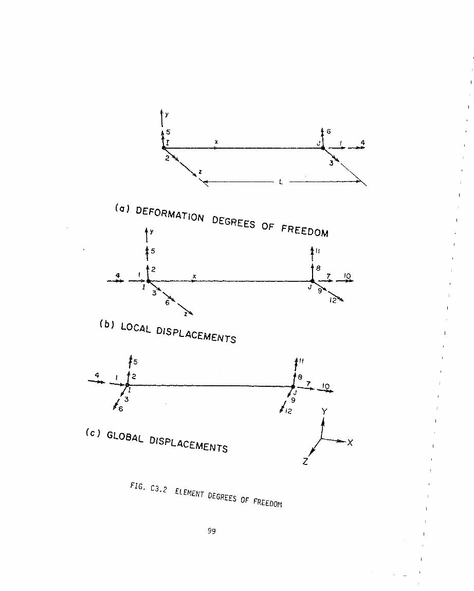
ty
J~~tk",--Z-:..:----l- 3 ~'~----
(0) DEFORMATION DEGREES OF FREEDOM
t'lk:~~
J 9 ..........li-....
(c) GLOBAL DISPLACEMENTS
z
FIG. C3.2 ELEMENT DEGREES OF FREEDOl1
99
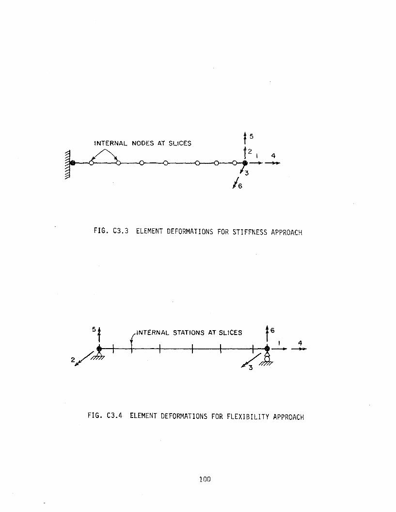
INTERNAL STATIONS AT SLICES
INTERNAL NODES AT SLICES
43i.---6---o----<:~-o_--_o_-o_-o_.. --+-~
FIG. C3.3 ELEMENT DEFORMATIONS FOR STIFFNESS APPROACH
t6
I 4....-4---4----+----+---;-----t-.-.~
FIG. C3.4 ELEMENT DEFORMATIONS FOR FLEXIBILITY APPROACH
100

D. EXAMPLES
This section describes a number of examples which have been used to test the straight
curved pipe and multi-slice tube elements.
101

Dl. PIPE WITH AXIAL FORCE AND INTERNAL PRESSURE
Dl.1. PURPOSE
The purpose of this example is to check the inelastic behavior of the pipe element under
combined axial and hoop sstresses and to verify that the Mroz material model has been
correctly implemented.
D1.2 CONFIGURAnON
A cantilever pipe as shown in Fig. D 1. I(a) is considered. The pipe length is lOO feet.
with 48-in. outside diameter and 0.6-in. wall thickness. The material stress-strain curve is
assumed to be trilinear, as shown in Fig. D1.l(b). Poisson's ratio is 0.3.
D1.3 ANSR ANALYSIS MODEL
D1.3.1 Assumptions for Analysis
The cantilever pipe was modeled by a single straight pipe element, with one end fixed and
the other free. The element was specified to have two Gauss points. Because no bending
moment exists, the pipe cross section was subdivided into only two subelements (fibers) around
the pipe circumference.
D1.3.2 Loadings
A uniform internal pressure of 864 psi was first applied. This pressure produced hoop and
axial stresses, with a von Mises effective stress just below yield. An axial tensile load of 2500
kips was then applied at the free end in five equal steps.
D1.3.3 ANSR Input
The ANSR-I1I input file for the example is listed in Table D 1.1.
Preceding page blank103
D1.4 RESULTS
The computed von Mises effective stresses and strains in the pipe wall are shown in Fig.
D 1.1 (b). All points lie on the "virgin" uniaxial stress-strain curve. The variation of axial stress
with axial strain is shown in Fig. D1.l(c).
These results were compared with the results obtained from the well-established pipeline
analysis program PIPLIN [D.11, which uses the Mroz theory but with a significantly different
computational scheme. The results from the two analyses were virtually identical.
D1.5 CONCLUSION
This example indicates that the pipe element gives correct results for inelastic behavior
under combined axial and hoop stresses and that the Mroz material model has been correctly
implemented.
104
D2. BURIED PIPE BEND WITH TEMPERATURE AND PRESSURE LOADING
02.1 PURPOSE
This example tests the inelastic behavior of the pipe element under temperature change,
internal pressure, and bending.
D2.2 CONFIGURATION
The structural configuration is shown in Fig. D2.1 (a). It represents a 12-degree, 120-f1.
radius sidebend in a pipeline, with virtual anchors (fixed supports) at both ends. The pipe is
modeled using straight and bend elements, with 48-in. outside diameter and 0.6-in. wall thick
ness. Because of symmetry, only one-half of the structure needs to be modeled, with a roller
support at the axis of symmetry. The pipe material stress-strain curve is assumed to be tri
linear, as shown inn Fig. D2.I(b). Poisson's ratio is 0.3, and the coefficient of thermal expan
sion 0.00001 per degree.
D2.3 ANSR ANALYSIS MODEL
D2.3.1 Assumptions of Analysis
The structure was modeled using six pipe elements, three straight elements for the
straight segment and three curved elements for the curved segment. Each element was
specified to have two Gauss points. The pipe cross section was divided into six subelements
(fibers) around one-half of the pipe circumference.
02.3.2 Loadings
A uniform temperature and internal pressure (equal values at all nodes) were applied to
the analysis model as follows.
(I) Apply internal pressure of 1750 psi in ten steps.
(2) Decrease internal pressure to zero in ten steps.
105
(3) Re-apply internal pressure to 1750 psi in ten steps.
(4) Apply k.nperature change of -100 degrees F in ten steps.
D2.3.3 ANSR Input
The ANSR-III input file for this example is listed in Table D 1.2.
D2.4 RESULTS
Load sequence (l) causes initial yiieJding of the pipe and causes outward movement of
the side bend (Fig. D2.2). After the pressure is removed in sequence (2), a small inward
deflection is present at the midpoint of the model (Fig. D2.2). Re-application of the internal
pressure in sequence (3) returns the sidebend segment back to the location at the end of
sequence (D. The temperature decrease then causes inward movement of the bend (Fig.
D2.2). The computed displacements are shown in Fig. D2.2 and the computed pipe moments
in Fig. D2.3. The corresponding results obtained using PIPLIN aTe also shown in Figs. D2.3
and D2.5. It can be seen that the results are in close agreement.
D2.5 CONCLUSION
The ANSR results are in agreement with those obtained by PIPLIN, which has been
widely used and carefully validated. This indicates that the pipe element is applicable for inelas
tic temperature and internal pressure loading.
106
D3. PIPE WHIP WITH LARGE DISPLACEMENTS
D3.1 PURPOSE
This example tests the straight-curved pipe element with large displacements and dynamic
loading.
D3.2 CONFIGURATION
Analyses of a cantilevered pipe with large displacements and impact have been reported
by Hibbitt and Karlsson [D.2l. The dimensions of the pipe are shown in Fig. 03.1.
ANSR-III V-bar elements are located at nodes 16 through 19, with initial gaps specified to
represent a flat surface. Each element is arbitrarily assigned a stiffness of 104 k/in, which
allows a small amount of flexibility after gap closure. In the analysis reported in fD.21, the flat
surface was assigned a very large mass, rather than an elastic stiffness. Because impact of an
actual pipe would involve substantial local deformation of the pipe, and probably significant
deformation of the impacted wall, the assumption of an essentially rigid surface is not realistic,
and the computed impact forces are likely to be much larger than those which would occur in
actual practice.
The analysis in [D.2l considered a "follower" jet force, acting parallel to line 19-20.
Because ANSR-III does not currently include a follower force option for dynamic loads, the
analysis was carried out assuming a vertical jet force. The results are thus not directly compar
able with those in [0.21, especially after impact. The straight-curved pipe element has also
been incorporated into WIPS [0.3], a special purpose computer code for pipe whip analysis. In
the verification studies for WIPS, a similar analysis has been carried out with a follower jet
force.
The stress-strain relationship for the pipe steel is shown in Table 03.1. The blowdown
forcing function is shown in Table 03.2.
107
D3.3 ANSR ANALYSIS MODEL
D3.3.1 Geometry. Loading. and Pipe Properties
The PIPE element subdivision is shown in Fig. D3.1. This is similar to the subdivision
used in [D.2J. It may be noted that only a single element is used in the vertical leg between
nodes 19 and 20. This introduces a significant error in the rotational inertia of this leg, and for
practical analysis a larger number of nodes is probably desirable.
Motion was permitted in the XY plane only. The default ovalling strengths and
stiffnesses were assumed for the curved PIPE elements, with small availing assumed. Twelve
subelements (the default value) were used in each PIPE element cross section.
The jet force was applied at node 20 in the vertical direction. To allow for the symmetry.
the jet forces shown in Table D3.2 were multiplied by 0.5 (because only half of the element
strengths and stiffnesses are used in symmetrical segments of the analysis moden.
D3.3.2 Analysis Control Parameters
The Newmark scheme with automatic time step selection was used, with the following
parameters.
Initial time step = 5 x 10⁻⁴ sec.
Minimum time step
Maximum time step
5 X 10⁻⁶ sec.
10-3 sec.
Initial {3 o/~.t = 0.1
Lower midstep tolerance 50 k
Upper midstep tolerance = 250 k
D3.3.3 ANSR Input
The ANSR-III input file for the example is listed in Table 03.3.
108
D3.4 RESULTS
Deflected shapes at several times are shown in Fig. 03.2. This figure demonstrates that
the computational scheme can consider very large displacements. No results are available for
confirmation that the analysis is correct. A more detailed comparison with the results from
[0.21 is presented in (D.31, using the WIPS version of the element.
The analysis required a total of 228 time steps, 107 up to gap closure at 0.106 seconds,
and 121 for the remaining 0.029 seconds. The maximum time step was 0.00100 seconds Gn
the period before gap closure) and the minimum step was 0.000125 seconds On the period
shortly after gap closure).
109

D4. INELASTIC MULTI-SLICE BEAM COLUMN
D4.1 PURPOSE
This example tests the multi-slice tube element for its ability to capture the inelastic cur
vature variation along a single beam-column member. Four different cases have been con
sidered, each with a different number of slices. The load-deflection relationships and the calcu
lated curvature variations are compared, to study how accurately the different cases predict the
member behavior. This is only a preliminary test of the multi-slice element. Further work is
needed to test the element thoroughly and to study its characteristics in detail.
D4.2 CONFIGURATION
The tubular beam-column shown in Fig. 04.1 (a) has its bottom end fixed and its top end
restrained by an elastic rotational spring. The spring stiffness of 42,650 k/radian is chosen so
that the bending moments at the top and bottom ends are in essentially the ratio 2: 1 in the elas
tic state. The material stress-strain curves for the pipe steel were as shown in Fig. 04.1 (bi.
Two different strain hardening ratios were considered for each model, namely 1% and .01%.
Four different models, each with a different number of slices, have been specified. The
num bers of slices and their locations are shown in Table 04.1.
D4.3 ANSR ANALYSIS MODEL
D4.3.1 Assumptions for Analysis
Each slice cross section was subdivided into 8 subelements (fibers) around one-half of the
pipe circumference (to account for symmetry only one-half of the beam-column strengths and
stiffnesses were used in the analysis modej).
For each model, a lateral displacement of 2.2 inches (approximately 4 times the yield dis
placement) was applied at the top end, in two increments. In the first increment a displacement
magnitude of 0.5 inches was applied in one step. This brought the beam-column close to first
yield. In the second increment a displacement of 1.7 inch was applied in twenty equal steps.
Preceding page blank 111
Constant displacement iteration was specified for all cases.
D4.3.2 ANSR Input
The ANSR-III input data file for the 7-slice model, with strain hardening 0.01 %, is listed
in Table D4.2. The remaining data files were similar and are not listed.
D4.4 RESULTS
D4.4.1 Expected Behavior
In the elastic range, the bending moment at the bottom of the member is 2.04 times that
at the top. Simple hand calculation shows that first yield occurs at a load of 3.33 k and a
deflection of 0.53 inches. (This load is on one-half of the member because symmetry is
assumed,)
After yield, redistribution of moment occurs, and the top moment increases more rapidly
than the bottom moment. For an elastic-perfectly-plastic material, the collapse load is reached
when plastic hinges form at both the top and bottom of the member. The plastic moment capa
city is 1.28 times the yield moment for a tubular section. Hence, the rigid-plastic collapse load
is 5.75 k.
No exact solution is available for the behavior between first yield and collapse. However,
a load-deflection relationship can be obtained assuming that ideal plastic hinges develop at the
member ends. With this assumption, a hinge forms at the bottom at a load of 0.28)(3.33) =
4.26 k. The stiffness then reduces to one-fourth the elastic value, until a hinge forms at the
top at the collapse load. The strength then remains constant. The load-deflection curve for this
simple "elastic-ideal-hinge" assumption is shown on the figures to provide a reference.
D4.4.2 Load Versus Deflection
The calculated load-deflection curves for a substantial strain hardening ratio (l %) are
shown in Fig. D4.2. The results for the seven- and nine-slice models are closely similar, and
are believed to be close to the "exact" behavior. The four-slice model gives reasonably accurate
112
results. However, the two-slice model gives poor results.
The load-deflectiion curves with negligible strain hardening ratio (0.01%) are shown in
Fig. 04.3. Again, the seven- and nine-slice models give closely similar results. In both of
these models, a plastic mechanism forms at approximately two inches deflection, with the
correct collapse strength. Note that the elastic-ideal-hinge model forms a mechanism at 1.84
inches deflection. The four-slice model again gives fair results, and the two-slice model gives
very poor results.
The reason why the two-slice model gives poor results is that the variation of cross section
flexibility between slices is obtained by linear interpolation. With only two slices, this provides
inaccurate values, and the element is much too flexible. With four slices, the flexibility varia
tion is estimated more accurately, but substantial error still exists. With either seven or nine
slices, the linear interpolation appears to give accurate results.
For the seven- and nine-slice models, the ultimate load capacity is some 3% larger than
that predicted for the elastic-ideal-hinge model. Approximately I% of this difference can be
attributed to strain hardening. The remaining difference occurs because the slice bending
moments in the multi-slice model do not lie exactly on a straight line. This is because the
shape function is recalculated only at discrete intervals, so that some error can develop. The
result is that the effective end bending moments (obtained by virtual work) are somewhat
larger than the bending moments on the end slices. The calculated strength is thus also slightly
too large. This aspect of the multi-slice model requires further study.
D4.4.3 Curvature Versus Deflection
The calculated curvatures at the top and bottom of the member are listed in Tables D4.3
and 04.4, for 1% and .01 % strain hardening, respectively. For each case the calculated curva
tures for the four-, seven-, and nine-slice models are of the same order of magnitude. How
ever, those for the two-slice model are much lower. This again indicates that the two-slice
model does not predict the inelastic deformation accurately. The four-slice model is also
113
significantly inaccurate, whereas the seven- and nine-slice models give closely similar results.
Note that the calculated curvatures with the elastic-plastic material (0.01 % strain harden
ing) are much larger than for the material with significant hardening (l%). This indicates that
material properties must be carefully specified if ductility demands based on curvature (or
strain) are to be calculated.
D4.5 CONCLUSION
This example, although limited in scope, suggests that the multi-slice element has the
ability to calculate accurate curvatures and load-deflection relationships for beam-column
members. The example suggests that a seven-slice model should be adequate for practical com
putation, and shows that calculated curvatures can be sensitive to the material stress-strain
curve.
Although the results are not shown here, an analysis was also performed with an
extremely low strain hardening ratio OO-Ill{>;o). For reasons which are not clear, the results
were poor for all cases <including seven and nine slices). Hence, it is recommended that if the
element is used, a strain hardening ratio of at least 0.01% be specified.
Additional study is needed 'to test the multi-slice element thoroughly and to develop
guidelines for its use. Time and resources have not been available to perform these additional
studies under the current project. Nevertheless, it can be concluded that the multi-slice con
cept is very attractive for modeling beam columns when curvature or strain ductilities are to be
calculated.
114
D5. SUMMARY
D5.1 GENERAL
This section has presented three examples using the straight-curved pipe element and one
example using the multi-slice beam-column element.
The examples with the straight-curved pipe element have all been carried out using the
ANSR-III computer code and have only exercised the element for two-dimensional behavior.
The element has also been incorporated into the WIPS code (D.3l. In the verification studies
for WIPS, the element was also exercised for three-dimensional behavior. However, these ana
lyses are not reported here.
The example with the multi-slice element is very limited in scope, exercising the element
only in two dimensions and ignoring axial force and torsion.
Elements such as those described in this report are very complex. Developing, testing
and documenting them is time-consuming and costly. Time and resources have not permitted
thorough testing. If the elements are used in practical applications, the analyst is cautioned to
perform additional tests to ensure that the elements are performing correctly.
115

D6. REFERENCES
D.l Structural Software Development, Inc., PIPLIN, Proprietary Computer Code and Documentation, Berkeley, California.
0.2 Hibbitt and Karlsson, Inc., "Analysis of Pipe Whip," Report EPRJ NP-12 08, Providence,Rhode Island, November 1979.
0.3 Powell, G. H. et aI, "WIPS: Computer Code for Whip and Impact Analysis of Piping Systerns," Report to Lawrence Livermore National Laboratory, Department of CivilEngineering, University of California, Berkeley, 1982 (to be published as a Nuclear Regulatory Commission NUREG document>.
Preceding page b!ank
117

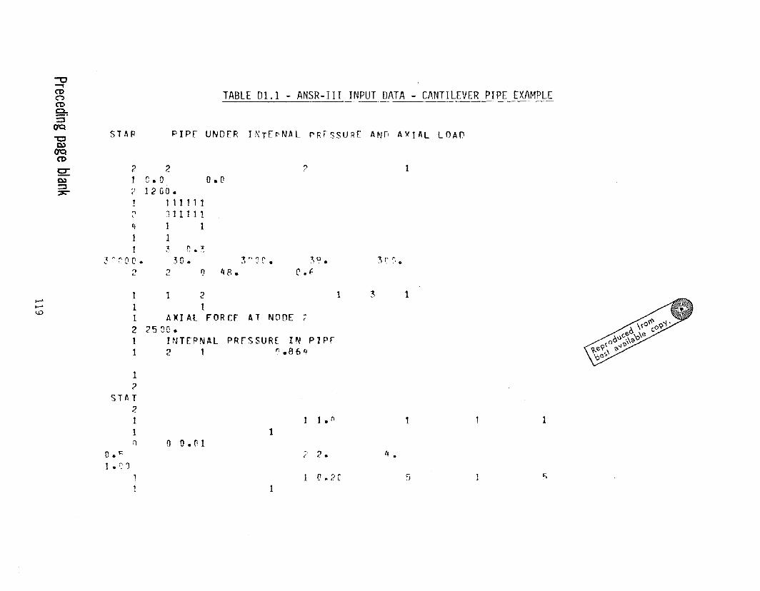
ST~R PIP[ UNDER I~TErNAL rRFsSURE ANn A~TAL LOAr
TABLE 01.1 - ANSR-III INPUT DATA - CANTILEVER PIPE EXAMPLE
I?O.C!
n .....,
2
:3
2411
21 C. 0;-' 12GO.
111111JIlll11 I1
-0~
('t)o('t)
~::;]
(7Q
"'C0)
Ot::l('D
cr0)::;]
="
3~;'OQ.
')L.. 2
,30.rJ 48.
'7 !"1 " f"l"I ,,-' \.. • ?:~ '? •
o•F:H ~'.
1 I 2 1I-'I-' I 11.0
1 AXIAL FORCE AT NODE ;:-
2 25 80.1 INTEPNAL PRfSSURE IN PIPfI 2 1 ".861;
:3 1
1?
STAT;?
1 ] 1 • n 11 1n 0 0.(11
o• t::., 2. II •"
1 • ~' D1 1 (1.2 C 51 1
1
s
•
•C\J
....o
• c>c:; •....
u-,•
Ci
wo..ZO01;;;: l/.l
120
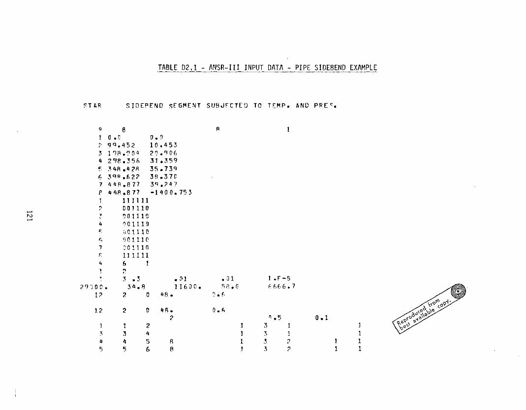
TABLE 02.1 - ANSR-III INPUT DATA - PIPE SIDEBEND EXAMPLE
~TAR SIDEPEND sfGMENT SU8JFCTEO TO T[MP. AND PRE <::.
Q 8 A
o•c 0.0? qq.'fS2 10.4533 19R.t?04 21].9064 2q8.356 31.359s:- ~ 4A .4 2R 35.73'1~I
r:, 3qQ.62? 38 .. 37C7 44R.A77 39.247r 44P..871 -1400.7531 111111? 001110.....
N ? 'JOllIe.......4 ~I01110
~ :JOII10r.. SC11H'7 ;01110r 1111114 6 1
?, 3 .3 .81 • J 1 1 • r-5
21]:;00. 34.8 116[)O. t:JH.O {'666.7
12 2 0 if 8 • J.f
12 2 0 ItR. D.F.2 1'\ .5 0.1
1 1 2 1 :3 1 13 3 4 1 3 1 14 1I 5 8 1 3 ? 1 1r; 5 6 8 1 3 ? 1 1
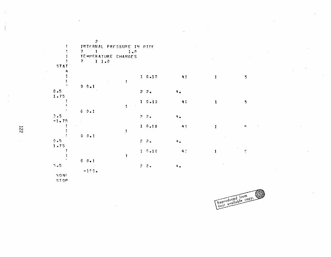
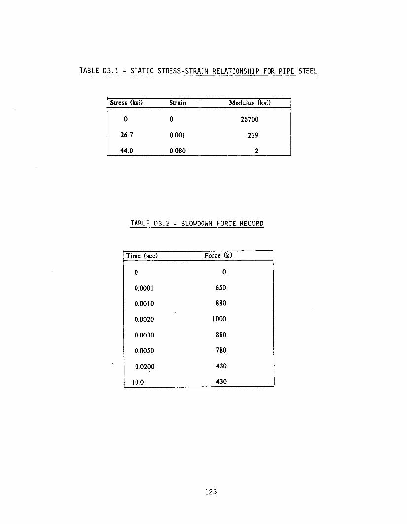
TABLE 03.1 - STATIC STRESS-STRAIN RELATIONSHIP FOR PIPE STEEL
Stress (ksj)
o
26.7
0«.0
Strain
o
0.001
0.080
Modulus (ksi)
26700
219
2
TABLE 03.2 - BLOWDOWN FORCE RECORD
Time (seC> Force (k)
0 0
0.0001 650
0.0010 880
0.0020 1000
0.0030 880
0.0050 780
0.0200 430
10.0 430
123
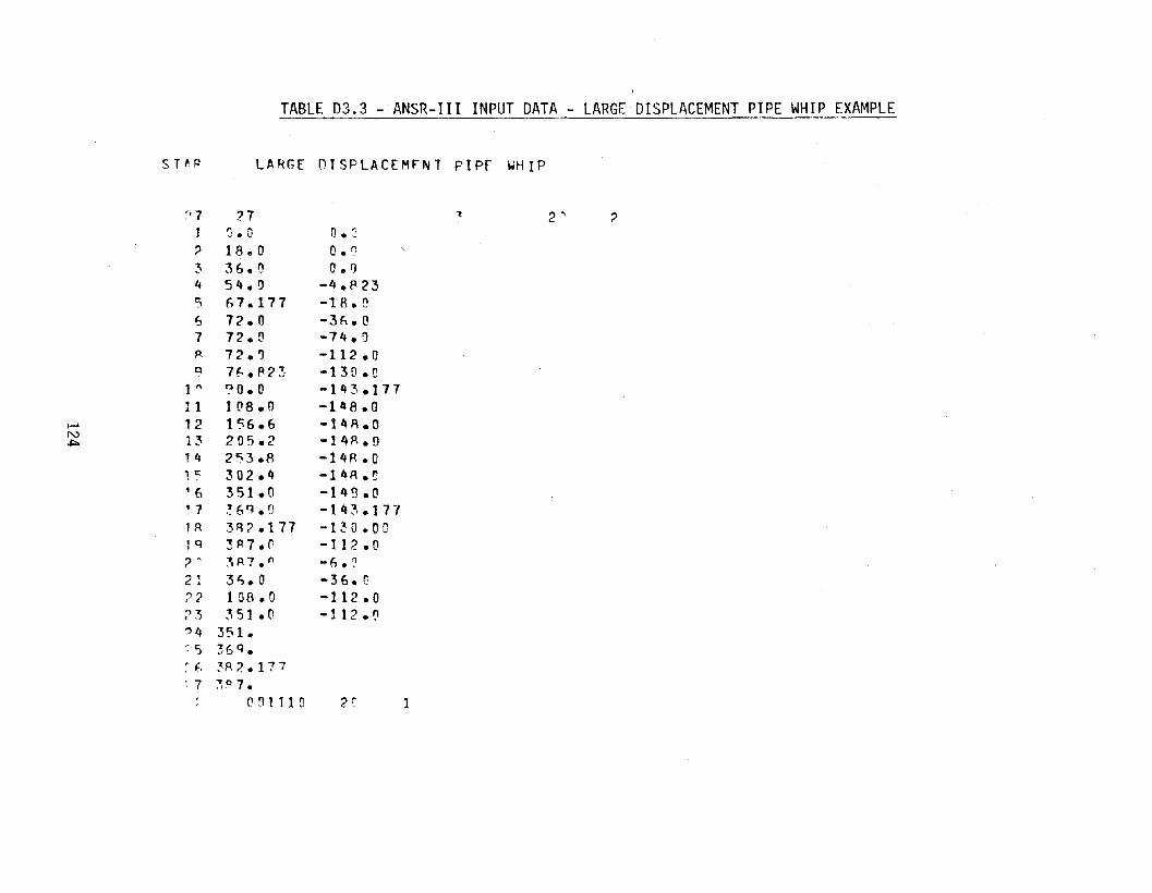
TABLE 03.3 - ANSR-III INPUT DATA - LARGE DISPLACEMENT PIPE WHIP EXAMPLE
S T!' P LA RGE OISPLACEMFNT PI pr IoiH IP
~17 27 "t 2 ., ')
J ~ • 0 o• ':, 18.0 o• 0
3 36.1) 0.1)4 54.!) -4.823'5 67.177 -1 H. !:'6 72.0 -3(,.07 72.0 -14.JP. 72.'1 -112 .09 U· .P23 -13D.1J
1 " ~O.O -143.17711 ](18.0 -148.0
I-' 12 156.6 -14A.ON
13 205.2 -14A.D.j::;:o
1 4 253.8 -14A .01 c: 302.4 -14A.1J1 f, 351.0 -149.Q'1 ~·6q.Q -143.1771A .3~;:>.177 -1~O.OC
1 q 3R7.0 -112.0,.~R7.'" -('.:'
2 1 3".0 -36. 0:'2 1 DB .0 -112.0~3 351 .0 -112.~
"4 351.~, ') 36q.~ .. r. ~A ? 1 7 7
~ 7 !. 07.(1~1110 2 C'
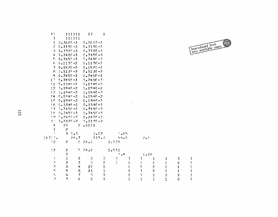
?: 111111 27 11 1111111 a.:'i6()~-3 (103~ CE-:3:> (I.719r~-3 0.719(-:',3 O.13?F -3 1J.732(-34 (1.745[-3 0.745E-3i; 0.745·-3 'l.745[-~
~ ').11 '3~-2 1J.11~E-?
7 Q.15 2E-2 1J.152".::-:'P. Q.1l3r--2 0.113E-:>'3 0.745[-3 O.74sr-3
1~ 'J.745 r -3 1J.745r-~,
U 0.134[-2 ~.1~4F:-?
! 2 :'l.lQ4[-2 0.1°4[-21 3 0.194·-2 0.194[-2! 4 C.1 Cl 4'-2 0.194(-2I ~ (!.1941'-2 O.194C::-:>1 [. [.134[-2 Q.134[-?
..... ~ 7 ~.745r-3 1J.745r-~
N 1 r. Q.745[-3 J.74Sr-:t,U1 • q r .'41)·-2 CI.2 4 °1'-:'
2 ~ G.?l?'-2 J.21 ?r-24 19 1 .00011 ?
3 C • ~ G.e? " .0 l)
'2f:.7[ ~. ';>(-.7 2I g. J 44.0 ? ri
, :> ? (' 2 II • C I • t:; : 1
~ ? ;> r 24.0 1.l):'tl~ n .4 (;.081 2 0 C " 1 1 1 1 0 1"
~ ;:> .3 ,j [1 " 1 1 1 1 0 1~ 3 4 21 1 1 1 2 1 1 1
.I.
r:; 5 ~ 21 1 I 1 ? 1 1 Ic) (, 7 '1 0 1 1 1 1 0 t7 7 8 0 0 1 1 1 1 0 1
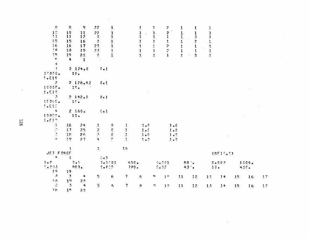
~\ 8 9 n 1 1 1 2 1 1 11 " 10 11 22 1 1 1 2 1 1 1l·
11 11 12 0 1 1 1 1 1 D 115 15 16 0 1 1 1 1 1 C 116 16 17 23 1 1 • :> 1 1 1~
! R 18 19 2~ 1 1 1 " 1 1 1..19 19 20 0 1 1 1 1 1 0 1~ ~ 14
1 2 124.0 C.l1I'ODC. 10.~.E10
? 2 12A.R2 0.11coer. 1C.I • El ']
3 2 142. a 0.1traGc. 1 r •~ • E 1 C
4 2 160. hIl')nr~l. 1 n•
....... 1 • r 1 ,.,NO"l 1 16 24 1 (1 1 1 • C 1.0
17 25 ') e 1 1 • C 1 .0'-., IP, 2" :. 0 1 1.0 1 • f)II 19 27 4 f', 1 ] • C! 1 • a
1 1 If,JET FOReE (fIF1r:.~)
Q 1 ~'. 50.(' a• IJ ~.Ol·Ol 650. ::; • C0 1 88 .• 0.002 1 COO.':.['·J3 88D. ~.(,:5 1PO. ~.O2 43'. 10. 43(1.
1 q 19:::> 3 4 5 (, 7 8 q 1 n 11 12 13 14 15 16 17
1 R tt) 2C''0 3 4 5 6 7 R g 1 '! 11 12 13 14 15 16 17<.
1R lq 20

I •
o•
C'v
o,.-:.
-c CJLI"l • •• 0a
r:;
-.L C\JW
•U"'. -c:> -<::> 0L' C'
• •0 U-' If').... I"'l 0 C\J-0
LJ"' • •c, 0 CI
0C' Co' r Lo-: 0.
Z CJ C-. .... Z ~.
>- 0 c 0 r0-
O • .-. Z V)e-
127
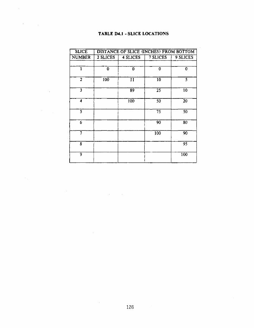
TABLE D4.1 - SLICE LOCATIONS
SLICE DISTANCE OF SLICE (INCHES) FROM BOTTOMNUMBER 2 SLICES 4 SLICES 7 SLICES 9 SLICES
1 0 0 0 0
2 100 11 10 5
3 89 25 10
4 100 50 20
5 75 50
6 90 80
7 100 90
8 95
9 100
128
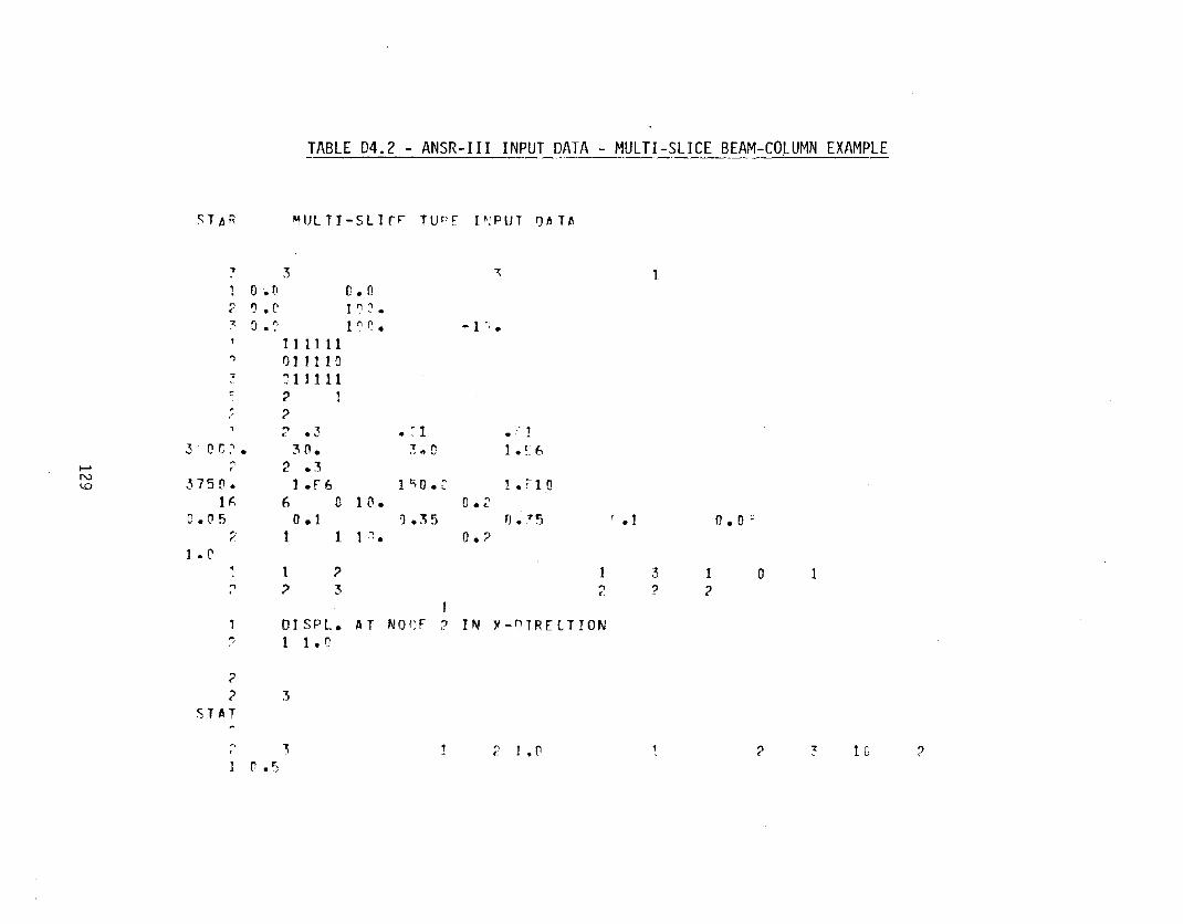
TABLE D4.2 - ANSR-III INPUT DATA - MULTI-SLICE BEAM-COLUMN EXAMPLE
~TAR ~ULTI-Sllr~ TUP[ I~PUT QAT~
7 3o •(I
;: o. C7, o. ':'
"1
<:
"
'>;
-1 '; •
ll:iO.: 1. rIO1 {l. 0.;'
1.:')5 rJ .75t"': • o.?
......N~
:3 () C" •
37S().1F.
O.(l5?
~ .330.
2 .31 • r 6
6 00.1
1 1
• ~ 1"' n.~ • oJ
.' I1 • !~ £,
r .1 o• 0 c
1 • C'
",1?
?3 "<.
3?
1;>
o 1
01 S PL. AT NO I: r ? IN Y- n TRE (T ION~ 1 1. Q
?? 3
STAT
", "3(l .5
2 1. (I 1 ? :: 1 G ?
u;o•
c· 0 c c'
• • • •.... .... ....
- .... ..,., ~,...•-
::'\. .- , ('., C.,; L... '-Z C
U"'l,.... 0 ~
• • &. v:= ....
130
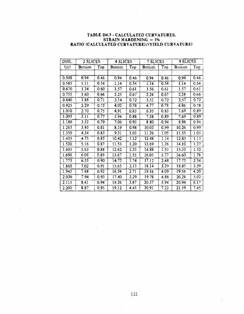
TABLE D4.3 - CALCULATED CURVATURES.STRAIN HARDENING = 1%
RATIO (CALCULATED CURVATURE)/(YIELD CURVATURE)
DISL. 2 SLICES 4 SLICES 7 SLICES 9 SLICES(in) Bottom Top Bottom Top Bottom Top Bottom Top
0.500 0.94 0.46 0.94 0.46 0.94 0.46 0.94 0.460.585 1.11 0.54 1.14 0.54 1.14 0.54 1.14 0.540.670 1.34 0.60 1.57 0.61 1.56 0.61 1.57 0.610.755 1.60 0.66 2.25 0.67 2.24 0.67 2.28 0.660.840 1.88 0.71 3.14 0.72 3.51 0.72 3.57 0.720.925 2.29 0.73 4.02 0.78 4.77 0.78 4.86 0.78
1.010 2.70 0.75 4.91 0.83 6.35 0.83 7.69 0.891.095 3.11 0.77 5.94 0.88 7.58 0.89 7.69 0.891.180 3.52 0.79 7.06 0.93 8.80 0.94 8.98 0.941.265 3.93 0.81 8.19 0.98 10.03 0.99 10.26 0.991.350 4.34 0.83 9.31 1.03 11.26 1.05 11.55 1.051.435 4.75 0.85 10.42 1.12 12.48 1.14 12.83 1.15
1.520 5.16 0.87 11.53 1.20 13.69 1.26 14.10 1.27
1.605 5.63 0.88 12.62 1.35 14.88 1.53 15.35 1.52
1.690 6.09 0.89 13.67 1.55 16.05 1.77 16.60 1.781.775 6.55 0.90 14.72 1.74 17.12 2.48 17.75 2.54
1.860 7.02 0.91 15.65 2.13 18.14 3.29 18.85 3.391.945 7.48 0.92 16.54 2.71 19.16 4.09 19.56 4.202.030 7.94 0.93 17.40 3.29 19.78 4.88 20.28 5.022.115 8.41 0.94 18.26 3.87 20.37 5.94 20.94 6.17
2.200 8.87 0.95 19.12 4.45 20.91 7.22 21.59 7.45 -
131
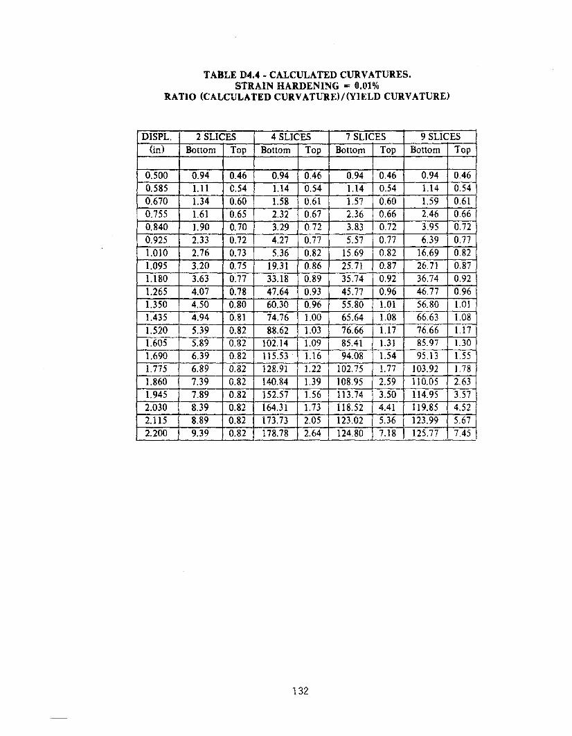
TABLE D4.4 • CALCULATED CURVATURES.STRAIN HARDENING == 0.01%
RATIO (CALCULATED CURVATURE)!(YIELD CURVATURE)
DISPL. 2 SLICES 4 SLICES 7 SLICES 9 SLICES(in) Bottom Top Bottom Top Bottom Top Bottom Top
0.500 0.94 0.46 0.94 0.46 0.94 0.46 0.94 0.460.585 1.11 0.54 1.14 0.54 1.14 0.54 1.14 0.540.670 1.34 0.60 1.58 0.61 1.57 0.60 1.59 0.610.755 1.61 0.65 2.32 0.67 2.36 0.66 2.46 0.66
0.840 1.90 0.70 3.29 0.72 3.83 0.72 3.95 0.72
0.925 2.33 0.72 4.27 0.77 5.57 0.77 6.39 0.77
1.010 2.76 0.73 5.36 0.82 15.69 0.82 16.69 0.82
1.095 3.20 0.75 19.31 0.86 25.71 0.87 26.71 0.87
1.180 3.63 0.77 33.18 0.89 35.74 0.92 36.74 0.92
1.265 4.07 0.78 47.64 0.93 45.77 0.96 46.77 0.961.350 4.50 0.80 60.30 0.96 55.80 1.01 56.80 1.011.435 4.94 0.81 74.76 1.00 65.64 1.08 66.63 1.081.520 5.39 0.82 88.62 1.03 76.66 1.17 76.66 1.171.605 5.89 0.82 102.14 1.09 85.41 1.31 85.97 1.30
1.690 6.39 0.82 115.53 1.16 94.08 1.54 95.13 1.551. 775 6.89 0.82 128.91 1.22 102.75 1.77 103.92 1.781.860 7.39 0.82 140.84 1.39 108.95 2.59 110.05 2.631.945 7.89 0.82 152.57 1.56 113.74 3.50 114.95 3.572.030 8.39 0.82 164.31 1.73 118.52 4.41 119.85 4.522.115 8.89 0.82 173.73 2.05 123.02 5.36 123.99 5.672.200 9.39 0.82 178.78 2.64 124.80 7.18 125.77 7.45
132
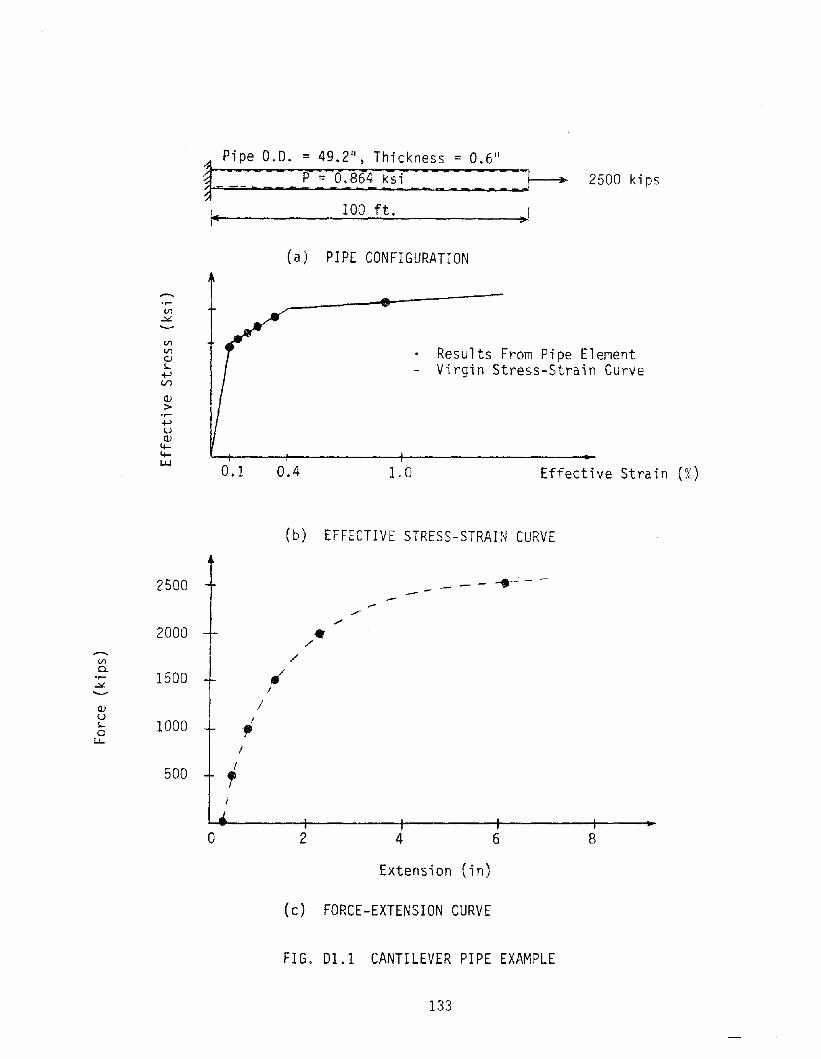
Pipe 0.0. = 49.2", Thickness = 0.6"
~: • ::: P :::0:,8!{ §i ::::-::::: :J--+ 2500 kips
I- 100 ft. ~,
(a) PIPE CONFIGURATION
. Results From Pipe Element- Virgin Stress-Strain Curve
V1V1ClJS~
V)
ClJ>~
uClJ
44l..LJ
0.1 0.4 1.0 Effective Strain (%)
V10......
ClJUSou...
2500
2000
1500
1000
500
/,/
I
r
//
(b) EFFECTIVE STRESS-STRAIN CURVE
....-- --- -
.../
/
o 2 4 6 8
Extension (in)
(c) FORCE-EXTENSION CURVE
FIG. 01.1 CANTILEVER PIPE EXAMPLE
133
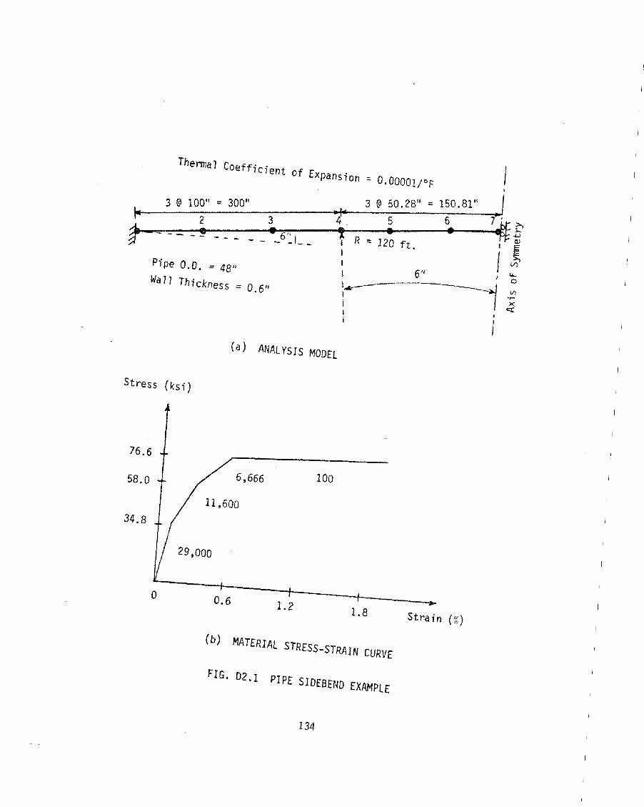
(/).......><"
Thermal Coefficient of Expansion
Pipe 0.0. ::: 48"
Wall Thickness::: 0.6"
I::: a.DDDOI/oF I
3 @ 50.2811::: 150.81 11 ..f~--':3~@~1~0~0::'11 "::::~30~O~II_3 :.~.r:.=~j5~===~6.:==q7~ €
"'::~~~2::~;=;=~~6":liT'::-::--1~I~Rl\::::-1~2~~~ft~'--""--/1 ,ll' ---- -~ - -'- - I 6" , :;;
IIIIIi
(a) ANALYSIS MODEL
Stress (ksi)
76.6
6,666 10058.0
11 ,60034.8
29,000
o 0.6 1.2 1.8 Strain (%)
(b) MATERIAL STRESS-STRAIN CURVE
FIG. 02.1 PIPE SIDEBEND EXAMPLE
134
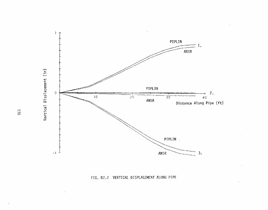
PIPLIN
ANSR1.
..-...t:::.,..
.........+Jt:::
PIPLINOJ
I 2.
E
°t~o, !
OJ
I !
40
uI
30
rt:I
20
Distance Along Pipe (ft)
..-
ANSR0..1Il,..
0
..-rt:IU...... .,..W+J(J1s..OJ
::>
PIPLIN
-1 3.
FIG. 02.2 VERTICAL DISPLACEMENT ALONG PIPE
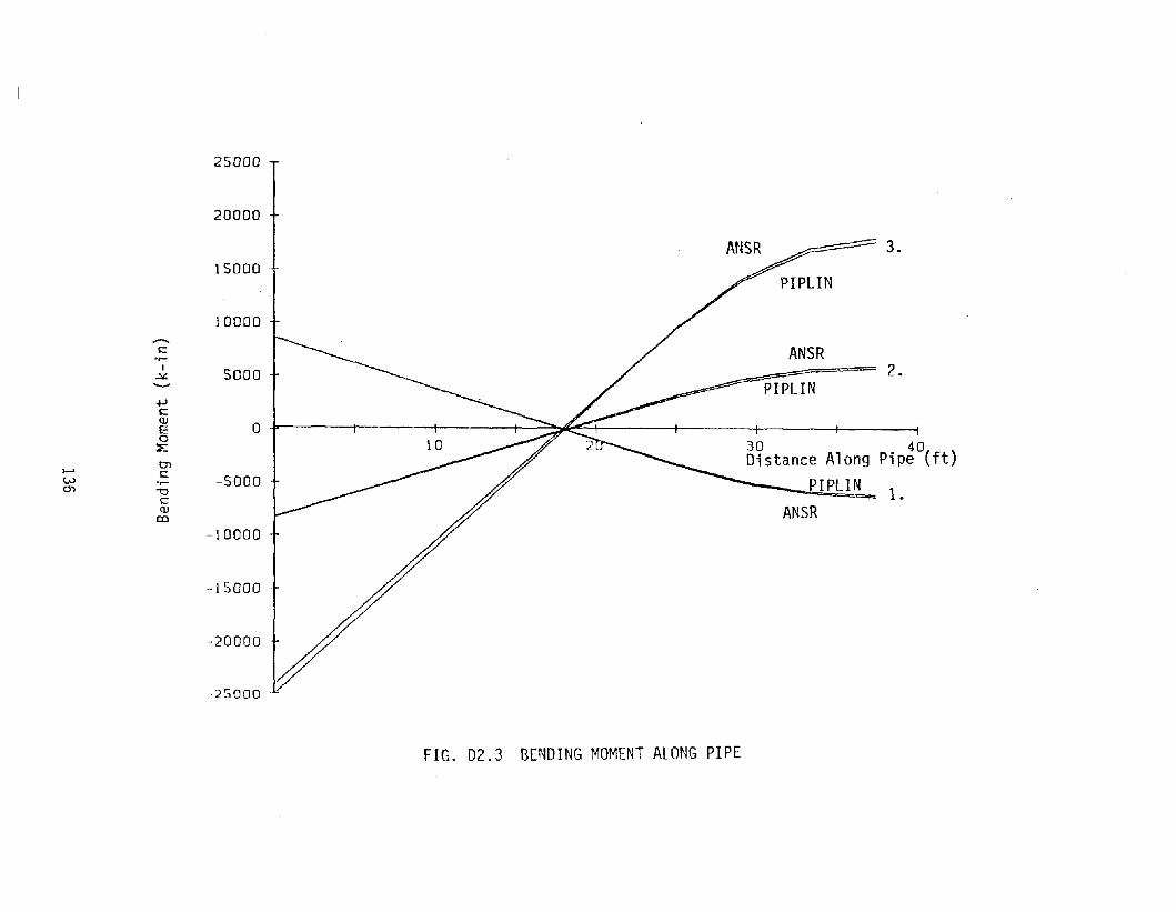
25000
20000II
3.15000
~
10000-c:or-
I 5000 1--------
/ = 2.~ --==.........pc:Q) aE0 10
-;7~ 2 30 40
...... 0'1 Distance Along Pipe (ft)c:w .... -soDa PIPLIN()) -0 l.c:Q) ANSR0)
-10000
-15000
·-20000
-25000
FIG. 02.3 BENDING MOMENT ALONG PIPE
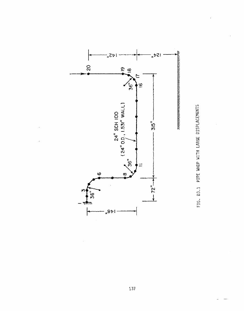
- (,/)...J r-...J zlJ.J0 <!::E:5: lJ.J0U= c::r:
J: -U') ...Jr-")0-U l{') r-") (,/)U) .......Cl
V lJ.J(.!}N0::c::r:...J
::I:r-.....::;:
0-..-.::I:::;:
<.D WJ0-......0-
-N ~.,....(')
Cl
-l .(.!}..-.W-
I~ ..817\ ~l
1--1t217 I ·1- 1t t721
0 (J) CDN~
<D
137
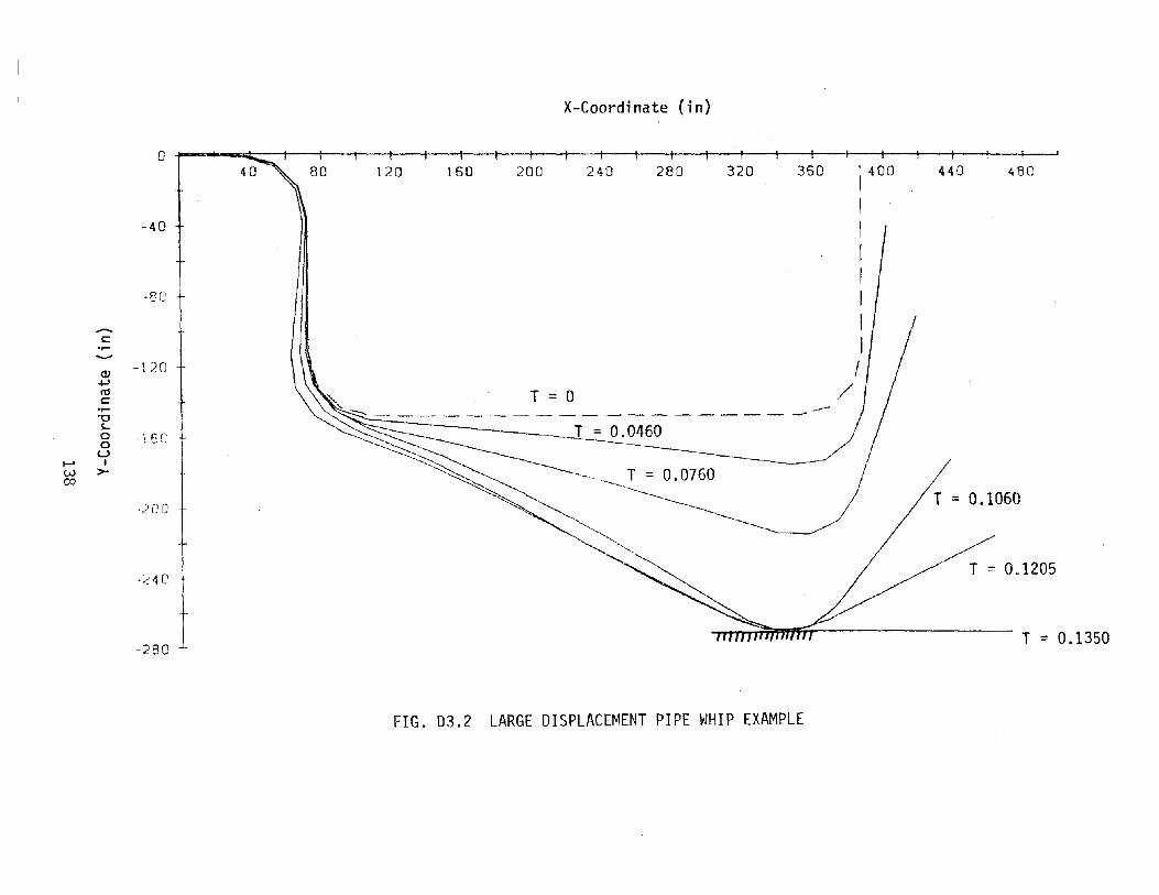
X-Coordinate (in)
o I I ~l I I I I I I I I I I I I I I , I I I I ! I I
440 480
T =0.1060
360320280240200160120 . 400IIIIIIIII
/--T=O _~ - - - - - -T~O.0460~~--- --------~~. - - T==0.0760~~--------- - .--------
80
-40
-eo
--c.~
........<V
-120+.J10C.~
"'0s-o - i r. (,0
.._,'..;
U...... IW >-co
-2 [; 0
-'" 4 C'
-280 -
T == 0.1205
T == 0.1350
FIG. 03.2 LARGE DISPLACEMENT PIPE WHIP EXAMPLE
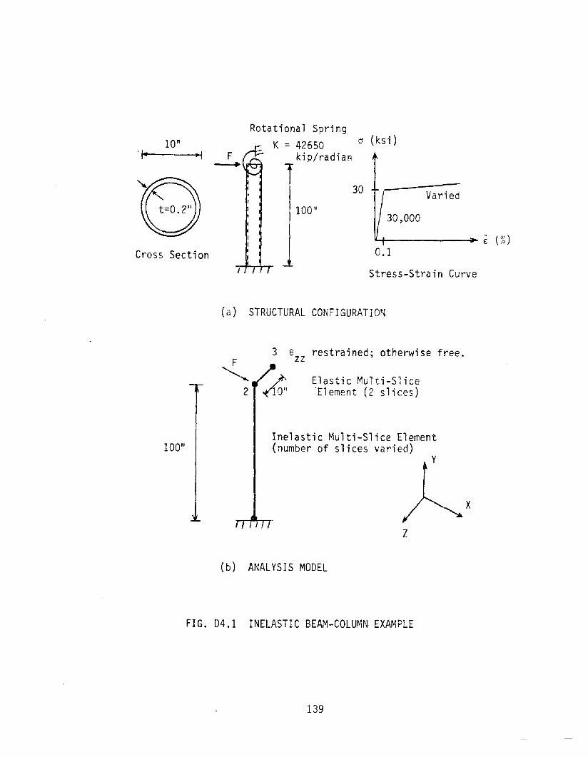
10"
Rotational SpringK = 42650
kip/radial1a (ks i)
100"
30 Varied
30,000
~------ E (%)Cross Section 0.1
Stress-Strain Curve
(a) STRUCTURAL CONFIGURATION
Elastic Multi-Slice-Element (2 slices)
3 8 restrained; otherwise free.zzF
"; ~,
laO"Inelastic Multi-Slice Element(number of slices varied)
Y
z
x
(b) ANALYSIS MODEL
FIG. 04.1 INELASTIC BEAM-COLUMN EXAMPLE
139
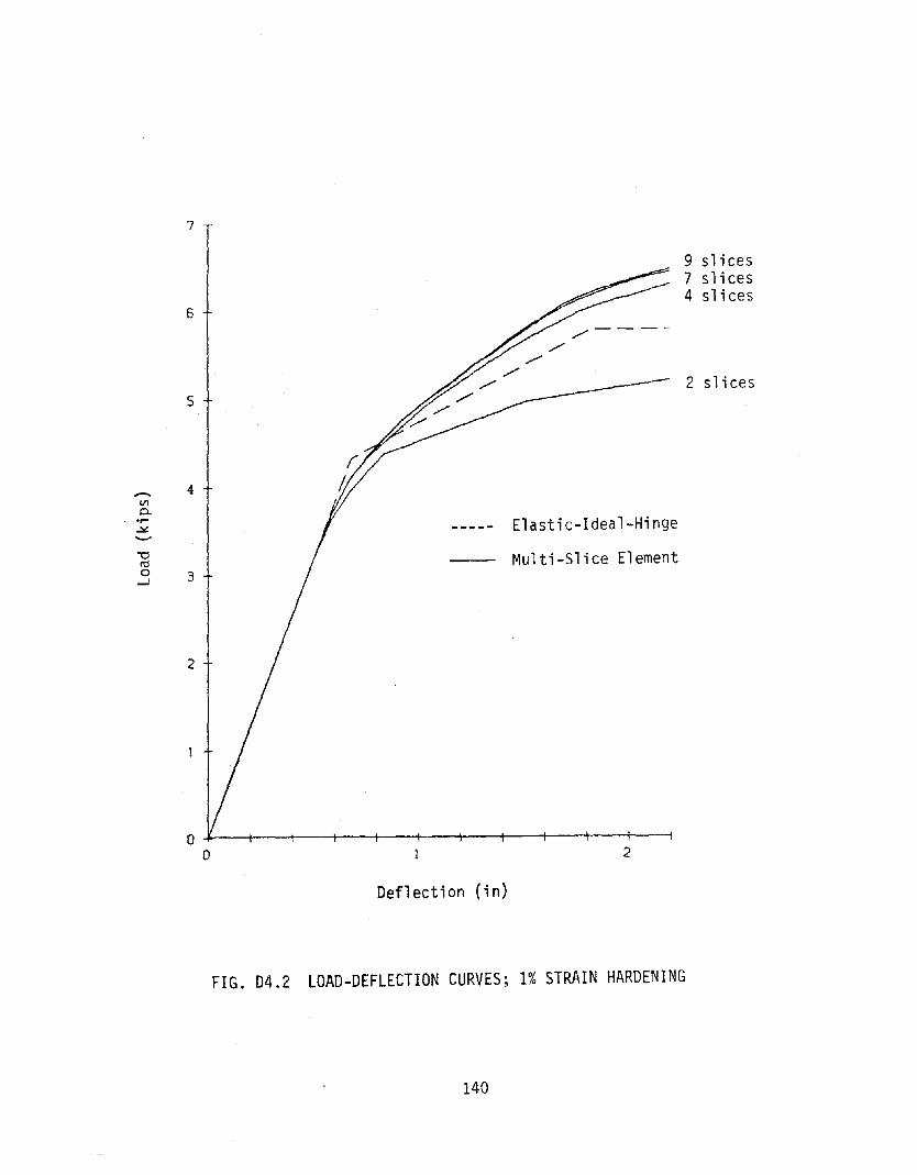
7
2 slices
9 slices7 slices4 slices
2
2
5
6
o........--+---t--t----1r----t-..-;---+--+--t----t---1o
....... 4III0-
o .r- Elastic-Ideal-Hinge~---"0 Multi-Slice Elementttl0 3-l
Deflection (in)
FIG. 04.2 LOAD-DEFLECTION CURVES; 1% STRAIN HARDENING
140
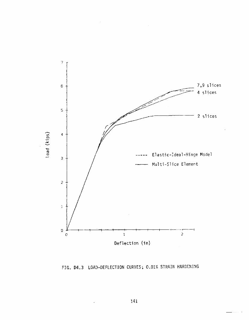
7
6
5
-til 40.
3
2
oo
Deflection (in)
7,9 slices4 slices
2 slices
Elastic-Ideal-Hinge Model
Multi-Slice Element
2
FIG. 04.3 LOAD-DEFLECTION CURVES; 0.01% STRAIN HARDENING
141

EARTHQUAKE ENGINEERING RESEARCH CENTER REPORTS
NOTE: Numbers in parentheses are Accession Numbers assigned by the National Technical Information Service; these arefollowed by a price code. Copies of the reports may be ordered from the National Technical Information Service, 5285Port Royal Road, Springfield, Virginia, 22161. Accession Numbers should be quoted on orders for reports (PB --- ---)and remittance must accompany each order. Reports without this information were not available at time of printing.The complete list of EERC reports (from EERC 67-1) is available upon request from the Earthquake Engineering ResearchCenter, University of California. Berkeley, 47th Street and Hoffman Boulevard, Richmond, California 94804.
UCB/EERC-77/01 "PLUSH - A Computer Program for Probabilistic Finite Element Analysis of Seismic Soil-Structure Interaction," by M.P. Romo Organista, J. Lysmer and H.B. Seed - 1977 (PB81 177 651))\05
UCB/EERC-77/02 "Soil-Structure Interaction Effects at the Humboldt Bay Power Plant in the Ferndale Earthquake of June7, 1975," by J.E. Valera, H.B. Seed, C.F. Tsai and J. Lysmer - 1977 (PB 265 795)A04
UCB/EERC-77/03 "Influence of Sample Disturbance on Sand Response to Cyclic Loading," by K. Mori, H.B. Seed and C.K.Chan - 1977 (FB 267 352)A04
UCB/EERC-77/04 "Seismological Studies of Strong Motion Records," by J. Shoja-Taheri - 1977 (FB 269 655)AIO
UCB/EERC-77/05 Unassigned
UCB/EERC-77/06 "Developing Methodologies for Evaluating the Earthquake safety of Existing Buildings," by 110. 1 -B. Bresler; No.2 - B. Bresler, T. Okada and D. Zisling; No.3 - T. Okada and B. Bresler; 110. 4 - V.V.Bertero and B. Bresler - 1977 (FB 267 354)A08
UCB/EERC-77/07 "A Literature Survey - :'ransverse Strength of Masonry Walls," by Y. Ornote, R.L. Mayes, S. W. C,en andR.W. Clough - 1977 (FB 277 933)A07
UCB/EERC-77/08 "DRAIN-TABS: A Computer Program for Inelastic Earthquake Response of Three Dinensional Buildings," byR. Guendelman-Israel and G.H. Powell - 1977 (PB 270 693)1'.07
UCS/EERC-77/09 "SUBWALL: A Special Purpose Finite Element Computer Program for Practical Slastic Analysi3 ~nd Desi~n
of Structural Nalls with Substructure Option, II by 0.'2. Le, H. Pecerson and :S.P. Popov - 1977(PB 270 567)A05
UCB/EERC-77/10 "Experimental Evaluation of Seismic Design Methods for Broad Cylindrical Tanks," by D.P. Clough(PB 272 280) AU
UCE/EERC-77/ll "Earthquake Engineering Research at Berkeley - 1976," - 1977 (FB 273 507)A09
UCE/EERC-77/12 "Automated Design of Earthquake Resistant Multistory Steel Build~ng Frames," by N.D. Walker, Jr. - 1977(FE 276 526)A09
UCB/EERC-77 /13 "Concrete Confined by Rectangular Hoops Subjected to Axial Loads," by J. Vallenas, V.V. Bertero andE.P. Fopov - 1977 (PB 275 165)A06
UCB/EERC-77/14 "Seismic Strain Induced in the Ground During Earthquakes," by 1. Sugimura - 1977 (PB 284 201),,04
UCB/EERC-77/1S Unassigned
UCB/EERC-77/16 "Computer Aided Optimum Design of Ductile Reinforced Concrete Moment Resist~ng Frames," by S. vi.Zagajeski and V.V. Bertero - 1977 (PB 280 137)A07
UCB/EERC-77/17 "Earthquake Simulation Testing of a Stepping Frame with Energy-Absorbing Devices," by J.t1. Kelly andD.F. Tsztoo - 1977 (PB 273 506)A04
UCE/EERC-77/1S "Inelastic Behavior of Eccentrically Braced Steel Frames under Cyclic Loadings," by C.W. Roeder andE.P. Popov - 1977 (PB 275 526)A15
UCB/EERC-77/19 "A Simplified Procedure for Estimating Earthquake- Induced Deformations in Dams and Embankments," by F. 1.Makdisi and H.B. Seed - 1977 (PE 276 820)A04
UCB/EERC-77/2C1 "The Performance of Earth Dams during Earthquakes," by H.B. Seed, F.r. Makdisi and P. de Alba - 1977(PB 276 821)1'.04
UCB/EERC-77/21 "Dynamic Plastic Analysis using Stress Resultant Finite Element formulation," by P. Lukkunapvasit andJ.M. Kelly - 1977 (PB 275 453)A04
UCB/EERC-77/22 "Preliminary Experimental Study of Seismic uplift of a Steel Frame," by R.W. Clough and A.A. Huckelbridge1977 (PB 278 769)A08
UCB/EERC-77/23 "Earthquake Simulator Tests of a Nine-Story Steel Frame with Columns Allowed to Uplift," by A.A.Huckelbridge - 1977 (PB 277 944)A09
UCB/EERC-77/24 "Nonlinear Soil-Structure Interaction of Ske·.... Highway Bridges," by M. -C. Chen andJ. Penzien - 1977(FB 276 176)A07
UCB/EERC-77/25 "Seismic Analysis of an Offshore Structure Supported on Pile Foundations," by D.D.-N. Liou and J. Penzien1977 (PB 283 180)A06
UCB/EERC-77/26 "!)ynamic Stiffness Matrices for Homogeneous ViscoelastiC Half-Planes," by~. Dasgupta and .".K. Chopra 1977 (PB 279 654)A06
Preceding page blank 143
UCB/EERC-77/27 "A Practical Soft Story Earthquake Isolation System," by J.M. Kelly, 3 .•\1. Eidinger and C.J. Derham _1977 (PB 276 814}A07
UCB/EERC-77/28 "Seismic Safety of Existing Buildings and Incentives for Hazard Mitigation in San Francisco: AnExploratory Study," by A.J. Meltsner - 1977 (PB 281 970)AOS
UCB/EERC-77/29 "Dynamic Analysis of Electrohydraulic Shaking Tables," by D. Rea, S. Abedi-Hayati and Y. Takahashi1977 (PB 282 S69}A04
UCB/EERC-77/30 "An Approach for Improving Seismic - Resistant Behavior of Reinforced Concrete Interior Joints," byE. Galunic, V.V. Bertero and E.P. Popov - 1977 (PB 290 870)1'1.06
UCB/EERC-78/01 "The Development of Energy-Absorbing Devices for Aseismic Base Isolation Systems," by J.M. Kelly andD.F. Tsztoo - 1978 (PB 284 978)A04
UCB/EERC-78/02 "Effect of Tensile Prestrain on the Cyclic Response of Structural Steel Connections, by J.G. Bouwkampand A. Mukhopadhyay - 1978
UCB/EERC-78/03 "Experimental Results of an Earthquake Isolation System using Natural Rubber Bearings," by J. ~1.
Eidinger and J.M. Kelly - 1978 (PE 281 686)1'1.04
UCB/EERC-78/:J4 "Seismic 8ehavior of Tall Liquid Storage Tanks," by A. Niwa - 1978 (PB 284 017)1'1.14
UCE/EERC-78/0S
UCB/EERC-78/06
UCB/EERC-78/Q7
lJCBIt:2RC-78/D8
UCB/EERC-78/09
\JCB/EERC-78/1Q
UCB/EERC- 7 8/11
UCB/EERC-78/12
UCB/EERC- 78/13
UCB/EERC-78/14
LTCB/EERC-78/1S
UCB/EERC-78/16
UCB/EERC-78/17
UCB/EERC-78/18
UCB/EERC-78/19
UCB/EERC-78/20
UCB/EERC-78/21
UCB/EERC-78/22
UCB/EERC-78/23
UCB/EERC-78/24
UCB/EERC-78/25
"Hysteretic Behavior 0 f ReInforced Concrete Columns Subjected to High .<;xial and Cyclic Shear :orces, 11
by S.W. Zagajeski, V.V. Bertero and J.G. BOUWkamp - 1978 (PB 283 85811'1.13
"Three Dimensional Inela.stic Frame Elements for the P-.NSR-! Program,1I by A. Ria.hi, D.G. Row :3.ndG.H. Powell - 1978 (PB 29S 75S)A04
"Studies of Structural Response to Earthquake Ground (-'lotion, U by O.A. Lopez and A.K. Chopra - 19'78(PB 282 790)AOS
"A Laboratory Study of the Fluid-Structure InteraC1:10n of Submerged Tanks and Caissons in Earthquakes, ,I
by R.C. Byrd - 1978 (PB 284 9S7)AG8
Unassigne'd
"Seismic Performance of Ncnst~uct'...lral and Secondary Structural Elements," by I. Sakamoto - 1978(PBal 154 593)1'1.05
1I~·1athematical t-1odelling of Hysteresis Loops for Reinforced concrete Columns, II by S. Nakata, T. Sprouland J. Penzien - 1978 (PB 298 274)A05
"Damageability in Existing Buildings," by T. Blejwas and B. Bresler - 1978 (PB 80 166 9781AOS
"Dynamic Behavior of a Pedestal Base Multistory Building," by R.M. Stephen, B.L. Wilson, J.G. Bouwkampand M. Button - 1978 (PB 286 650)1'1.08
"Seismic Response of Bridges - Case Studies," by R.A. Imbsen, V. Nutt and J. Penzien - 1978(PB 286 S03)AIO
"A Substructure Technique for Nonlinear Static and Dynamic Analysis," by D.G. Rowand G.H .. Powell 1978 iPB 288 077)AIO
"Seismic Risk Studies for San Francisco and for the Greater San Francisco Bay Area," by C.. S. Oliveira 1978 (PS 81 120 115)AD7
"Strength of Timber Roof Connections Subjected to Cyclic Loads," by P. GUlkan, R.L. Mayes and R.W.Clough - 1978 (HUD-OOO 1491)A07
"Response of K-Braced Steel Frame Models to Lateral Loads," ~y J.G. Bouwkamp, R.M. Stephen andE.P. Popov - 1978
"Rational Design Methods for Light Equipment in Structures Subjected to Ground Motion," byJ.L. Sackman and J.M. Kelly - 1978 (PB 292 357)A04
"Testing of a Wind Restraint for Aseismic Base Isolation," by J.M. Kelly and D.E. Chitty - 1978(PB 292 833)A03
"APOLLO - A Computer Program for the Analysis of Pore Pressure Generation and Dissipation in HorizontalSand Layers During Cyclic or Earthquake Loading," by P.P. Martin and H.B. Seed - 1978 (PB 292 835)A04
"Optimal Design of an Earthquake Isolation System," by M.A. Bhatti, K.S. Fister and E. Polak - 1978(PB 294 73S)A06
"MASH - A Computer Program for the Non-Linear Analysis of vertically Propagating Shear Waves inHorizontally Layered Deposits," by P.P. Martin and H.B. Seed - 1978 (PB 293 101)A05
"Investigation of the Elastic Characteristics of a Three Story Steel Frame Using System Identification,"by I. Kaya and H.D. McNiven - 1978 (PB 296 22S)A06
"Investigation of the Nonlinear Characteristics of a Three-Story Steel Frame Using SystemIdentification," by I. Kaya and H.D. McNiven - 1978 (PE 301 363)A05
144
UCB/EERC-78/26 "Studies of Strong Ground Motion in Taiwan," by Y.M. Hsiung, B.A. Bolt and J. Penzien - 1976(PB 298 436).1\06
rJCB/EERC-78/27 "Cyclic Loading Tests of c.lasonry Single Piers: Volume 1 - Height to I'hdth Ratio of 2," by P ,A. Hidalgo,R.L. ~ayes, H.D. ~cNiven and R.W. Clough - 1976 (PS 296 211).1\07
'JCB/ESRC-78/28 "Ci'clic Leading Tests of Ylasonry Single Piers: Vol tune 2 - Height ~o Width Ratio ofP.A. Hidal.go, R.L. Mayes, R.',v, Clough and H.D. ~1cNiven - 1978 (PS 296 212).1\09
'; tl~, by S.-W.J. Chen,
'-'C3/EERC-78/29 "~.nal'!tL:al ;orocedures i.n Soil Dynamics," by J. Lysme1C - 1978 (FB 298 445)';06
UC3/EERC-79/01 "Hysteret~c Behavior 0 f Lightweight R:ir.forced Conc::ete Beam-Colulnn Subassemblages, " by B. Forzani,E.P. Popov and V.V. Bertero - April 1979(PB 298 267)A06
liCB/EERC-79/02 "The Development of a Mathematical Model to Predict t."e Flexural Response of Reinforced Concrete Beamsto Cyclic Loads, Usir.g System Identification," by J. Scanton & H. McNiven - Jan. 1979(PS 295 875)A10
UCB/EERC-79/03 "Linear and ~onlinear Earthquake Response of Simple Torsionally Coupled Systems," by C.L. Kan andA.K. Chopra - Feb. 1979(PB 298 262)A06
:';C3/EERC-79/04 lOA :vlat~ematical .YkJdel of MasonrJ for Predicting its Linear Seismi8 ResFOnse Characteristics, It byY. ~engi and H.D. McNiven - ?eb. 1979(PS 298 266)A06
:JCB/EERC-79/0S "~·1echanical Behavior of Lightweight Concrete Confined by Different Types of Lateral Reinforcement, II
by M.A. Manrique, V.V. Bertero and E.P. Popcv - May 1979(PS 301 114)A06
CCB/EERC-79/C6 "Static Tilt Tests of a Tall Cylindrical Liquid Storage Tank," by R.W. clough aDd rl. ::riwa - Feb. 1979(;OS 301 167) A06
:;CB/EEF.C- 79/D7 liThe 'Design of Steel Energy Absorbir.g Restrainers and Their Incor;:>oration into Nuclear Po\.;er Plantsfor Enhanced Safety: Volume 1 - SumInary ReI?Ort," by ?N. Spencer, V.F. zackay, and E.R. Parker Feb. 1979(UCB/EERC-79/07)A09
iJC3/EERC-79/08 HThe Design of Steel Energy hbsorbing Restrainers a:-:c. Their Incorporation into Nuclear PeHer Plantsfor Enhanced Safety: Volume 2 - The Jevelopment 0: A......alyses for R.eactor system piping,""SimFle Systems"by ~'1.C. Lee, J. Penzien, A.:-:. Chopra and K, Suzuki 1(Comolex Syste~srl by C.H. Powell, E.L. Hilson,R.W, Clough and D,G. Rcw - ?eb. 1979(GCS/EERC-79/08)A10
UCB/EERC-79/09 "The Design of Steel Energy ~bsorbing Restrainers and Their Incorporation into Nuclear Power Pl~~ts
for Enhanced~Sa£ety: Volume 3 - Evalt~ation of Commercial Steels," by W.S. 0..;eo, R.M.N. Pellol.\'x,R.O. Ritchie, ~1. Faral, T. Ohhashi, J. Toplosky,. S.J. !iartman, V.F. Zackay and E.R. Parker-?eb. 1979 (UCB/EERC-79/09) ,0.04
UCBiEEP.C-79/10 "The Design of Steel Energy Absorbing Restrainers and Their Incor?oration into Nuclear Power Plantsfor E!"'~'1anced Safety: Volume 4 - A Review of Energy-Absorbing Devices," by J. M. Kelly andM.S. Skinner - Feb. 1979(UCB/EERC-79/10)A04
UCB/EERC-79/11 "Conservatism In Summation "ules for Closely Spaced ~10des," by J. M. Kelly and J. L. Sackman - May1979(PB 301 328)A03
uCB/EERC-79/12 "Cy-:::lic :.oading Tests of ~'lasonry Single Piers; iJoltL'T!e 3 - Height to :~idt.~ Ratio of ;J.5," byP.A. Hidalgo, R.L. Mayes, H,D. McNiven and R,W. Clough - May 1979(PS 301 321)A08
CCS/EERC- 79/13 "Cyclic Behavior of Dense Course-Grained ~late::ials in Relation ::0 me Seismic S tabili ty of Dams," by'l.G. Banerjee, H.B. Seed and C.K. Chan - June 1979(PS 301 373).0.13
UCB/EERC-79/14 "Seismic Behavior of Reinfo::ced Concrete Interior Beam-Col umn Subassemblages," by S. Viwathanatepa,E.? Popov and V.V. Be::tero - June 1979(PS 301 326)';:0
GCB/EERC-79/l5 "Optlmal Design of Localized Nonlinear Systems wit." Dual Performance CriCeria Under EarthquakeExciCations," by M.~.. Shatt~ - July 1979(PB 80 167 l09)A06
UCB/EERC-79/16 "OPTDYN - A General Purpose Optimization Proqram for Problems wi t.'1 or wi thout Dynamic Cons craints,"by M.A. Bhatti, E. Polak and K.S. Pister - July 1979(PS 80 167 091)A05
UCB/EERC-79/17 ";""'lSR-II, Analysis of Nonlinea!" Structural Response, Users Manual," by D.P. Mond'<:ar and G.H. PowellJuly 1979(PS 80 113 301)A05
UCB/EERC-'i9/18 "Soil Structure Interaction in Different Seismic Environments," A. Gomez-Masso, J. Lysmer, J.-C. C:.~en
and H.B. Seed - August 1~79(PB 60 101 520)A04
UCB/EERC-79/19
UCB/EERC-79/20
UCB/EERC-79/21
UCB/EERC-79/22
UCB/EERC-79/23
UCB/EERC-79/24
"AR.'!A ~dels for Earthquake Ground Motions," by M.K. Chang, J.W. Kwiatkowski, R.F. Nau, R. .'!. Oliverand K.S. Pister - July 1979(PB 301 166)';05
"Hysteretic Behavior of Reinforced Concrete Structural Walls," by J. M. vallenas, V. V. Bertero andE.? Popov - August 1979(PB 80 165 905)Al.2
"Studies on High-F!"equency Vibrations of Buildings - 1: The Column Effect." by J. Lubliner - August 1979(PB 80 158 553)';03
"Effects of Generalized Loadings on Sond Reinforcing Bars Embedded in Confined Concrete Blocks," byS. Viwathanatepa, E.P. Popov and V.V. Be::tero - August 1979(PB 81 124 018)A14
"Shaking Table Study of Single-Stor! Masonry Houses, Volume 1 : Test Structures 1 and 2, " by P. GUlka..'1,R.L. Mayes and R.W. Clough - Sept. 1979 (HUD-OOO l763)A12
lIShaking Table Study of Single-Story ,lasonry Houses, volume 2 : Test Structures 3 and 4, " by P. Gulkan,R.L. ,!ayes and R.W. Clough - Sept. 1979 (HUD-OOO 1836)A12
UCB/EERC-79/25 "Shaking Table Study of Single-Stor! Masonry Houses, Volume 3: Summary, Conclusions and Recommendations,"by R.W. Clough, R.L. Mayes and P. Gulkan - Sept. 1979 (HUD-OOO 1837)A06
145
UCB/EERC-79/26 "Recommendations tor a U.S. -Japan Cooperative Research Program Utilizing Large-Scale Testing Facilities ,"by U.S.-Japan Planning Group - Sept. 1979(PB 301 407)A06
UCB/EERC-79/27 "Earthquake-Induced Liquefaction Near Lake Amatitlan, Guatemala," by H.B. Seed, I. Arango, C.K. Chan,A. Gomez-Masso and R. Grant de Ascoli - Sept. 1979(tWREG-CRlJ41)A03
UCB/EERC-79/28 "Infill Panels; Their Influence on Seismic Response of Buildings," by J .1'1. Axley and 'J. V. BerteroSept. 1979(PB 80 163 371)AlO
UCB/EERC-79/29 "3D Truss Bar Element (Type 1) for the ANSR-II Program," by D.P. Mondkar and G.H. Powell - Nov. 1979(PB 80 169 709) A02
UCB/EERC-79/30 "20 Beam-COlumn Element (Type 5 - Parallel Element Theory) for the ANSR-II Program," by D.G. Row,G.H. Powell and D.P. Mondkar - Dec. 1979(PB 80 167 224)A03
UCB/EERC-79/31 "3D Beam-Column Element (Type 2 - Parallel Element Theory) for the ANSR-II Program," by A. Riahi,G.H. Powell and D.P. Mandkar - Dec. 1979(PB 80 167 216)A03
UCB/EERC-79/32 "On Response of Structures to Stationary Excitation," by A. Der Kiureghian - Dec. 1979(PB 80166929) A03
UCB/EERC-79/33 "Undisturbed Sampling and cyclic Load Testing of Sands," by S. Singh, H.B. Seed and C.K. ChanDec. 1979(ADA 087 298/A07
UCB/EERC-79/34 "Interaction Effects of Simultaneous Torsional and Compressional Cyclic Loading of Sand," byP.M. Griffin and W.N. Houston - Dec. 1979(ADA 092 352)A15
UCB/EERC-8G/Ol "Earthquake Response of Concrete Gravity Dams Including Hydrodynamic and Foundation Inten.ctlonEffects," by A.K. Chopra, P. Chakrabarti and S. Gupta - Jan. 1980(AD-A087297)AIO
UCB/EERC-BO/02 "Rocking Response of Rigid Blocks to Earthquakes," by C.S. Yim, A.K. Chopra and J. Penzien - Jan. 1980(PBBO 166 002)A04
UCB/E2RC-80/03 "Optimum Inelastic Design 0 f Seismic-Resistant Reinforced Concrete Frame Structures, II by .3. ~v. Zagaj eskl.and V.V. Bertero - Jan. 1930(PB80 164 635)A06
UCB/EERC-BO/04 "Effects of Amount and Arrangeme~t of Wall-Panel Reinforcement on Hysteretic Behavior of ReinforcedConcrete Halls," by R. Ili'la and V.'J. Bertero - Feb. 1980(PBBl 122 525),,09
UC3/EERC-80/0S "Shaking Table Research on Concrete Dam "todels," by.'.. Niwa and R. 'tJ. Clough - Sept. 1980! PB8l 122 368) A06
UCB/"EERC-80/06 "The Design of Steel Snergy-Absorbing Eestrainers and their Incorporation into Nuclear PO'.-:er ?lants forEnhanced Safety (VoIlA): ?iping ~ith Energy Absorbing Restrainers: Parameter Study on S~all Systems,"by G.H. Powell, C. Ouqhourlian and J. Simons - June 1980
UCB/EERC-80/07 "Inelastic Torsional Response of Structures Subjected to Earthquake Ground Motions," by Y. YamazakiApril 1980(PB81 122 327)AOB
UCB/EERC-80/08 "Study of X-Braced Steel Frame Structures Under Earthquake Simulation," by Y. Ghanaat - April 19BO(PB81 122 335)All
UCB/EERC-80/09 "Hybrid Modelling of Soil-Structure Interaction," by S. Gupta, T.W. Lin, J. Penzien and C.S. YehMay 19BO(PBBl 122 319)A07 .
UCB/EERC-80/10 "General Applicability of a ;.lonlinear t10del of a One Story Steel frame," by B.1. Sveinsson andH.D. McNiven - May 1980(PB81 124 877)A06
;JCB/EERC-80/11 "A Green-Function l1ethod :or I'lave l;nteraction with a Submerged Body," by W. Kioka - April 1980(PBBl 122 269)A07
UCB/EERC-80/12 "Hydrodynamic Pressure and Added 1lass for Axisymmetric Bodies," by F. Nilrat - "lay 19BO (PBSl 122 343) A08
UCB/EERC-BO/13 "Treatment of Non-Linear Drag Forces Aoting on Offshore Platforms," by B.V. Dao and J. PenzienMay 1980(PB81 153 413)A07
UCB/EERC-80/14 "2D Plane/Axisymmetric Solid Element (Type 3 - Elastic or Elastic-Perfectly Plastic) for the ANSR-IIProgram," by D.P. Mondkar and G.H. Powell - July 1980(PB81 122 350)A03
UCB/EERC-BO/15 "A Response Spectrum Method for Random Vibrations," by A. Der Kiureghian - June 19BO (PBBl 122 301) A03
UCB/EERC-80/16 "Cyclic Inelastic BUCkling of Tubular Steel Braces," by V.A. Zayas, E. P. Popov and S. A. :·IahinJune 19BO(PBBl 124 385)AIO
UCB/EERC-80/17 "Dynamic Response of Simple Arch Dams InclUding Hydrodynamic Interaction," by C.S. Por"Cer andA.K. Chopra - July 19~0(PB81 124 000)A13
UCB/EERC-BO/18 "Experimental Testing of a Friction Damped Aseismic Base Isolation System with Fail-SafeCharacteristics," by J.M. Kelly, K.E. Beucke and M.S. Skinner - July 1980(PBSl 148 595)A04
UCB/EERC-80/19 "The Design of Steel Energy-Absorbing Restrainers and their Incorporation into Nuclear Power Plants forEnhanced Safety (Vol IB): Stochastic Seismic Analyses of Nuclear Power Plant Structures and PipingSystems Subjected to Multiple Support Excitations," bv M.C. Lee and J. Penzien - June 1980
UCB/EERC-80/20 "The Design of Steel Energy-Absorbing Restrainers and their Incorporation into ;.luclear POwer Plantsfor Enhanced Safety (Vol lC): Numerical Method for Dynamic Substructure Analysis," by J.M. Dickensand E.L. Wilson - June 1980
UCB/EERC-80/2l "The Design of Steel Energy-Absorbing Restrainers and their Incorporation into Nuclear Power Plantsfor Enhanced Safety (Vol 2); Development and Testing of Restraints for Nuclear Piping Systems," byJ.M. Kelly and M.S. Skinner - June 1980
UCB/EERC-80/22 "3D Solid Element (Type 4-Elastic or Elastic-Perfectly-Plastic) for the ANSR-II Program," byD.P. Mondkar and G.H. Powell - July 19BO(PBBl 123 242)A03
UCB/EERC-BO/23 "Gap-Friction Element (Type 5) for the ANSR-II Program," by D.P. Mondkar and G.H. Powell - July 1980(PB81 122 285)A03
146
UCB/EERC-80/24 "U-Bar "estraint Element (Type 11) for the ANSR-II Program," by C. Oughourlian and G.H. PowellJuly 1980(PB81 122 293)A03
UCB/EERC-80/25 "Testing of a Natural Rubber Sase Isolation System by an Explosi'Jely Simulated Earthquake," byJ.~. Kelly - August 1980(PB81 201 360)A04
UCB/EERC-80/26 "Input Identification from Structural Vibrational Response," by Y. Hu - August 1980(PB81 152 308);"05
UCB/EERC-30/27 "Cyclic Inelastic Behavior of Steel Offshore Structures," by V.A. Zayas, S.A. l1ahi!l and E.? PopovAugust 1980(PB81 196 180)A15
UCS/EERC-30/28 "Shaking Table Testing of a Reinforced Concrete Frame 'Hi th Biaxial Response," by 11. G. alivaOCtober 1980(PB81 154 304)AIO
UCB/EERC-80/29 "Dynamic Properties of a Twelve-Story Prefabricated Panel Building," by J.G. Bouwk=p, J.P. Kolleggerand R.I1. Stephen - October 1980(PB82 117 128)A06
UCB/EERC-80/30 "Dynamic Properties of an Eight-Story Prefabricated. panel Building," by J. G. Bouwkamp, J.P. Kolleggerand R.M. Stephen - October 1980(P881 200 313)A05
UCB/EERC-80/31 "Predictive Dynamic Response of Panel Type Structures Under Earthquakes," by J.P. Kollegg"r andJ.G. Bouwkamp - October 1980(PB81 152 316)A04
UC3/EERC-80/32 "7he Jesign of Steel Energy-Absorbing Restrainers and their Incorporation into Nuclear Power Plantsfor Enhanced Safety (Vol 3): Testing of :orr,tnerc:ial Steels in LOI,';-C'lcle Torsional Fatigue," byP. c~~~~~r, E.R. Parker, E. Jongewaard ~nd M. Drory
UCB/E=:'RC-30/33 "T:le L:}e~ign of Steel Enerqy-,~sorbing Restrainers a:1d their Incorporation into Nuclear POwdr Plants':or Enhanced Safety (Vol c.l): Shaking Table Tests of Piping SysteMS 'with Energy-Absorbinq Rest~ainers,"
by S.? Stiemer and W.~. Godden - Sept. 1980
UC3/EERC-30/34 "The 8esign of Steel Energy-AlJsorbir.g Restrainers an.j their Incor'poration into Nuclear Power Plantsfor Erthanced Safety (\101 S): Summary Report," by P. Spencer
IJC3/EERC-8C/35 "Experimental Testing of de Energy-Absorbing Base Isolation System, II by ... \~ Kelly, >1. S. S~ir.ner 3.r.d~.E. 3eucke - October 198C(?B81 15~)72)AO~
~CB/:SERc-aO/3o "Simulat.ing and f1.nalyzing .~,~tificidl Non-Stationary 2arthquake G:cound ~lotions," by F.. F. Nau, R.:·L Oliverand K.S. Pister - October 1980(P881 153 397jA04
UC8/EE?C-80/37 "Earthquake Engineering at Berkeley - 1980," - Se"t. 1980(PB81 2':;53-:'4) A09
CCS/2ERC-8C/38 "Inelastic Seismic .i\nalysis of Large Panel Buildings," by V. Schr-icker and C.H. Powell - Sept. 1980(PB81 154 338)A13
UCB/EE;<'C-80/39 "Synamic Response of Embankment, Concrete-Gravity and P.rch Dams Including Hydrodynamic Interaction,"by J.F. Hall and A.K. Chopra - October 1980(PB81 152 324)All
UCB/EERC-80/40 "Inelastic Buckling of Steel Struts Under Cyclic Load Reversal," by R.G, Black, W.A. Wenger andE.P, Popov - October 1980(PB81 154 312)A08
UCB/EERC-80/41 "Inflaence of Site Characteristics on Building Damage During the October 3, 1974 Lima Earthquake," byP. Repetto, I. Arango and H.B. Seed - Sept. 1980(PB81 161 739)A05
UCS/EERC-80/42 "Evaluation of a Shaking Table Test Program on Response Behavior of a ~NO Story Reinforced ConcreteFrame," by J.M. Blondet, R.~v. Clough and S.A. ~1ahin
UCB/EERC-80/43 ":r!odelling of Scil-Structu:ce Interaction by Finite and Infinite Elerr:ents, II by _. ~'1edina December 1980(P881 229 270jP.04
UCB/EERC-8l/01 "Control of Seismic Response of Piping Systems and Other Structures by Base Isolation," edited by J.~.
Kelly - January 1981 (PB8l 200 735)A05
UCB/EERC-81/02 "OPTNSR - An Interactive Software System for Optimal Design of Statically and Dyna~ically LoadedStructures with Nonlinear Response," by M.A. Bhatti, V. Ciampi and K.S. Pister - ,Tanuary J.981(PB81 218 851)A09
UCB/EERC-81/03 "Analysis of Local Variations in Free Field Seismic Ground l1otions," by J.-C. Chen, J. Lysmer and H.B.Seed - January 1981 (AD-A099508)A13
UCB/EERC-81/04 "Inelastic Structural Modeling of Braced Offshore Platforms for Seismic Loading," by V.A. Zayas,P.-S.B. Shing, S.A. Mahin and E.P. Popov - January 1981(PB82 138 777)A07
UCB/EERC-81/05 "Dynamic Response of 'Light Equipment in Structures," by A. Der Kiureghian, J.L. Sackman and 3. NourOmid - April 1981 (PB81 218 497)A04
UCB/EERC-81/06 "Preliminary Experimental Investigation of a Broad Base LiqUid Storage Tank," by J.G. Bouwkamp, J.P.Kol1egger and R.M. Stephen - May 1981(PB82 140 385)A03
UCB/EERC-81/07 "The Seismic Resistlant Design of Reinforced Concrete Coupled Structural 'lialls," by .J<. E. Aktan and V, V.Bertero - June 1981(PB82 113 358)All
UCB/EERC-81/08 "The Undrained Shearing Resistance of Cohesive Soils at Large Deformations," by M.R. P:/les and H.B.Seed - August 1981
UCB/EERC-8l/09 "Experimental Behavior of a Spatial Piping System with Steel Energy Absorbers Subjected to a SimulatedDifferential Seismic Input," by S.F. Stiemer, W.G. Godden and J.M. Kelly - July 1981
147
UCB/EERC-Bl/lO "Evaluation of Seismic Design Provisions for Masonry in the United States," by B. 1. Sveinsson, R.L.Mayes and H.D. McNiven - August 1981
UCB/EERC-8l/1l "'l'.lo-Dimensional Hybrid Modelling of Soil-Structure Interaction," by T. -J. Tzong, S. Gupta and J.Penzien - August 1981(PBB2 142 11B)A04
UCB/EERC-81/12 "Studies on Effects of Infills in Seismic Resistant RIC Construction," by S. Brokken and V.V. Bertero september 1981
UCB/EERC-81/13 "Linear Models to Predict the Nonlinear Seismic Behavior of a One-Story Steel Frame," by H. Valdimarsson,A.H. Shah and H.D. McNiven - September 1981{PB82 138 793)A07
UCB/EERC-8l/l4 "TLUSH: A Computer Program for the Three-Dimensional Dynamic Analysis of Earth Dams," by T. Kagawa,L.H. Mejia, H.B. Seed and J. Lysmer - September 1981(PB82 139 940)A06
UCB/EERC-8l/l5 "Three Dimensional Dynamic Response Analysis of Earth Dams," by L.H. Mejia and H.B. Seed - September 1981{PB82 137 274)A12
UCB/EERC-81/16 "Experimental Study of Lead and Elastomeric Dampers for Base Isolation Systems," by J.M. Kelly andS.B. Hodder - October 1981 (PB82 166 l82)A05
UCB/EERC-81/l7 "The Influence of Base Isolation on the Seismic Response of Light Secondary Equipment," by J.M. Kelly April 1981 {PB82 255 266)A04
UCB/EERC-8l/lB "Studies on Evaluation of Shaking Table Response Analysis Procedures," by J. Marcial Blondet - November1981 (PB82 197 27s)A10
UCB/EERC-8l/l9 "DELIGHT.STRUCT: A Computer-Aided Design Environment for Structural Engineering," by R.J. Balling,K.S. Pister and E. Polak - December 1981 (PBB2 218 496)A07
UCB/EERC-8l/20 "optimal Design of Seismic-Resistant Planar Steel Frames," by R.J. Balling, V. Ciampi, K.S. Pister andE. Polak - December 1981 (PB82 220 l79)A07
UCB/EERC-82/01 "Dynamic Behavior of Ground for Seismic Analysis of Lifeline Systems," by T. Sato and A. Der Kiureghi~ January 1982 (PB82 218 926)A05
UCB/EERC-82/02 "SluLking Table Tests of a Tubular steel Frame Model,~ by Y. Ghanaat and R. W. Clough - January 1982(PB82 220 161)A07
UCBjEERC-82/03 "Experimental Behavior of a Spatial piping System with Shock Arrestors and Energy Absorbers underseismic Excitation," by S. Schneider, H.-M. Lee and G. W. Godden - May 1982
UCB/EERC-82/04 "New Approaches for the Dynamic Analysis of Large Structural systems," by E. L. Wilson - June 1982(PB83 148 080)A05
UCB/EERC-82/05 "Model Study of Effects of Damage on ti,e Vibration Properties of Steel Offshore Platforms," byF. Shahrivar and J. G. Bouwkamp - June 1982
UCB/EERC-82/06 "States of the Art and Practice in the Optimum Seismic Design and Analytical, Response Prediction ofRiC Frame-Wall Structures," by A. E. Aktan and V. V. Bertero - July 1982 (PB83 147 736)A05
UCB/EERC-82/07 "Further Study of the Earthquake Response of a Broad Cylindrical Liquid-Storage Tank Model," byG. C. Manos and R. W. Clough - July 1982 (PB83 "'47 744)All
UCB/EERC-82/08 "An Evaluation of the Design and Analytical Seismic Response of a Seven Story Reinforced ConcreteFrame - Wall Structure," by F. A. Charney and V. V. Bertero - July 1982
UCB/EERC-82/09 "Fluid-structure Interactions: Added Mass Co:!!putations f'or Incompressible Fluid," by J. S.-H. Kuo August 1982
UCBjEERJ:-82/l0 "Joint-opening Nonlinear Mechanism: Interface Smeared Crack Model," by J. S.-H. Kuo August 1982 (PB83 149 195)A05
UCB/EERC-82/ll "Dynamic Response Analysis of Techi Dam," by R. W. Clough, R. M. Stephen and J. S.-H. Kuo August 1982 (PB83 147 496)A06
UCB/EERC-B2/12 "Prediction of the seismic Responses of RiC Frame-Coupled Wall Structures," by A. E. Aktan, V. V.Bertero and M. piazza - August 1982 {PB83 149 203~09
UCB/EERC-B2/13 "Preliminary Report on the SMART 1 Strong Motion Array in Taiwan," by B. A. Bolt, C. H. Loh, J.Penzien, Y. B. Tsai and Y. T. Yeh - AugUst 1982
UCB/EERC-82/l4 "Shaking-Table StUdies of an Eccentrically X-Braced Steel Structure," by M. S. Yang - September1982
UCB/EERC-82/15 "The Performance of Stairways in Earthquakes," by C. Roha, J. W. Axley and V. V. Bertero - september1982
148
UCB/EERC-82/16 "The Behavior of Submerged Multiple Bodies in Earthquakes," by W.-G. Liao - September 1982
Uca/EERC-82/17 "Effects of Concrete Types and Loading Conditions on Local Bond-Slip Relationships," by A. D. Cowell,E. P. Popov and V. V. Bertero - September 1982
UCB/EERC-82/18 "Mechanical Behavior of Shear Wall Vertical Boundary Members: An Experimental Investigation," byM. T. Wagner and V. V. Bertero - October 1982
UCB/EERc--82/19 "Experimental StUdies of Multi-support Seismic Loading on Piping systems," by J. M. Kelly andA. D. Cowell - November 1982
Uca/EERC-82/20 "Generalized Plastic Hinge Concepts for 3D Beam-Column Elements," by P. F.-S. Chen and G. H. Powell November 1982
UCB/EERC-82/2l "ANSR-III: General Purpose Computer Program for Nonlinear Structural Analysis," by C. V. Oughourlianand G. H. Powell - November 1982
UCB/EERC-82/22 "Solution Strategies for Statically Loaded Nonlinear Structures," by J. W. Simons and G. H. Powell November 1982
UCB/EERC-82/23 "Analytical Model of Deformed Bar Anchorages under Generalized Excitations," by V. Ciampi, R.Eligehausen, V. V. Bertero and E. P. Popov - November 1982
UCB/EERC-82/24 "A Mathematical Model for the Response of Masonry Walls to Dynamic Excitations," by H. Sucuoglu,Y. Mengi and H. D. McNiven - November 1982
UCB/EERC-82/25 "Earthquake Response Considerations of Broad Liquid Storage Tanks," by F. J. Cambra - November 1982
UCB/EERC-82/26 "Computational Models for cyclic Plasticity, Rate Dependence and Creep," by B. Mosaddad and G. H.Powell - November 1982
UCB/EERC-82/27 "Inelastic Analysis of Piping and Tubular Structures," by M. Mahasuverachai and G. H. powell - November1982
149