industrial power and automation lab manual · reliable, low latency, high speed communications over...
TRANSCRIPT

Department of Electrical Enggineering National Institute of Technology Calicut
INDUSTRIAL POWER AND AUTOMATION LAB MANUAL
NATIONAL INSTITUTE OF TECHNOLGY CALICUT NITC CAMPUS P.O. CALICUT
KERALA. PIN-673601 AUGUST 2011

Department of Electrical Engg. National Institute of Technology Calicut
POWER ENGINEERING LABORATORY
MANUAL
NATIONAL INSTITUTE OF TECHNOLGY CALICUT
NITC CAMPUS P.O. CALICUT
KERALA. PIN-673601
JULY 2009
Department of Electrical Engg. National Institute of Technology Calicut
List of Experiments
Experiment
I SCADA Experiments
a) Experiments on Transmission Module
Local Mode
1. Simulation of Faults
1.1 Line to Ground Faults (LG)
1.2 Line to Line Faults (LL)
1.3 Line to Line to Line Faults (LLL)
1.4 Line to Line to Ground Faults (LLG)
1.5 Line to Line to Line to Ground Faults (LLLG)
2. Ferranti Effect
3. Transmission Line Loading
1.1 Resistive Loading
1.2 Inductive Loading
1.3 Resistive and Inductive Loading
4. Transformer Loading
1.1 Resistive Loading
1.2 Inductive Loading
1.3 Resistive and Inductive Loading
5. VAR compensation
1.1 Series Compensation
1.2 Shunt Compensation
6. Sudden Load Rejection
Remote Mode
1. Simulation of Faults
1.1 Line to Ground Faults (LG)
1.2 Line to Line Faults (LL)
1.3 Line to Line to Line Faults (LLL)
1.4 Line to Line to Ground Faults (LLG)
2. Ferranti Effect
3. Transmission Line Loading
1.4 Resistive Loading
1.5 Inductive Loading
1.6 Resistive and Inductive Loading
4. Transformer Loading
Department of Electrical Engg. National Institute of Technology Calicut
1.4 Resistive Loading
1.5 Inductive Loading
1.6 Resistive and Inductive Loading
5. VAR compensation
1.3 Series Compensation
1.4 Shunt Compensation
6. Sudden Load Rejection
7. Operation of OLTC Transformer
b) Experiments on Distribution Module
Local Mode
1. Relay Co-ordination
2. PF Control/Voltage Regulation
3. Transformer Loading
Remote Mode
1. Relay Co-ordination
2. PF Control/Voltage Regulation
3. Transformer Loading
4. Demand Side Management
II Programmable Logic Controller Experiments
1. Speed Control of AC Servomotor
2. Batch Process Reactor Control
3. Lift Control
III Variable Frequency Drive Experiments
1. Comparison of Performance of Centrifugal Pump by Throttling
and Variable Frequency drive
IV Microcontroller Experiments
1. 80196 Experiments
1.1 Generation of PWM Signal
1.2 Generation of Saw-Tooth Signal
2. 8051 Experiments
2.1 Generation of PWM Signal
2.2 Generation of Saw-Tooth Signal

Department of Electrical Engg. National Institute of Technology Calicut
V DSP Experiments
1. Speed Control of Motor Using Digital Signal Processor
VI Power Quality Testing Experiments
1. Investigation on Power Quality Issues of Motor Under
Different Starting Conditions
2. Testing of UPS with Non Linear Loads
VII Eddy Current Drive Experiments
VIII Distributed Control System Experiments

Department of Electrical Engg. National Institute of Technology Calicut
SCADA Experiments
Introduction
ELECTRICAL power is one of the most important infrastructure inputs necessary for the
rapid economic development of a country. The ever-rising demand of electrical energy has led to
the installation and incorporation of a large number of electrical power generation units, with
increased capacities in a common power grid, making the operation of the entire system sensitive
to the prevailing conditions. Therefore, the extensive and complex power systems have become
unmanageable using the conventional instrumentation and control schemes. Intelligent systems
based on microprocessors and computers have been employed for online monitoring and control
of modern large-scale power systems, in generation, transmission and distribution, thereby
overcoming the complexities and drawbacks of the conventional instrumentation schemes.
The term “Automation”
Automation is the use of scientific and technological principles in the manufacture of
machines that take over work normally done by humans. This definition has been disputed by
professional scientists and engineers, but in any case, the term is derived from the longer term
“automatization” or from the phrase “automatic operation”. Delmar S. Harder, a plant manager
for General Motors, is credited with first having used the term in 1935.
History of Automation
Ideas for ways of automating tasks have been in existence since the time of the ancient
Greeks. The Greek inventor Hero (fl. about A.D. 50), for example, is credited with having
developed an automated system that would open a temple door when a priest lit a fire on the
temple altar. The real impetus for the development of automation came, however, during the
Industrial Revolution of the early eighteenth century. Many of the steam-powered devices built
by James Watt, Richard Trevithick, Richard Arkwright, Thomas Savery, Thomas Newcomen,
and their contemporaries were simple examples of machines capable of taking over the work of
humans. One of the most elaborate examples of automated machinery developed during this
period was the draw loom designed by the French inventor Basile Bouchon in 1725. The
instructions for the operation of the Bouchon loom were recorded on sheets of paper in the form
of holes. The needles that carried thread through the loom to make cloth were guided by the
presence or absence of those holes. The manual process of weaving a pattern into a piece of cloth
through the work of an individual was transformed by the Bouchon process into an operation that
could be performed mindlessly by merely stepping on a pedal.
Automation Applications
Manufacturing companies in virtually every industry are achieving rapid increases in
productivity by taking advantage of automation technologies. When one thinks of automation in
manufacturing, robots usually come to mind. The automotive industry was the early adopter of
robotics, using these automated machines for material handling, processing operations, and
Department of Electrical Engg. National Institute of Technology Calicut
assembly and inspection. Donald A. Vincent, executive vice president, Robotic Industries
Association, predicts a greater use of robots for assembly, paint systems, final trim, and parts
transfer will be seen in the near future.
One can break down automation in production into basically three categories: fixed
automation, programmable automation, and flexible automation. The automotive industry
primarily uses fixed automation. Also known as "hard automation," this refers to an automated
production facility in which the sequence of processing operations is fixed by the equipment
layout. A good example of this would be an automated production line where a series of
workstations are connected by a transfer system to move parts between the stations. What starts
as a piece of sheet metal in the beginning of the process, becomes a car at the end.
Programmable automation is a form of automation for producing products in batches. The
products are made in batch quantities ranging from several dozen to several thousand units at a
time. For each new batch, the production equipment must be reprogrammed and changed over to
accommodate the new product style.
Flexible automation is an extension of programmable automation. Here, the variety of
products is sufficiently limited so that the changeover of the equipment can be done very quickly
and automatically. The reprogramming of the equipment in flexible automation is done off-line;
that is, the programming is accomplished at a computer terminal without using the production
equipment itself.
Computer numerical control (CNC) is a form of programmable automation in which a
machine is controlled by numbers (and other symbols) that have been coded into a computer.
The program is actuated from the computer's memory. The machine tool industry was the first to
use numerical control to control the position of a cutting tool relative to the work part being
machined. The CNC part program represents the set of machining instructions for the particular
part, while the coded numbers in the sequenced program specifies x-y-z coordinates in a
Cartesian axis system, defining the various positions of the cutting tool in relation to the work
part.
SCADA
SCADA is an acronym that stands for Supervisory Control and Data Acquisition. SCADA
refers to a system that collects data from various sensors at a factory, plant or in other remote
locations and then sends this data to a central computer which then manages and controls the
data. SCADA is a term that is used broadly to portray control and management solutions in a
wide range of industries. SCADA generally refers to an industrial control system: a computer
system monitoring and controlling a process. The process can be industrial, infrastructure or
facility based as described below:

Department of Electrical Engg. National Institute of Technology Calicut
� Industrial processes include those of manufacturing, production, power
generation, fabrication, and refining, and may run in continuous, batch, repetitive, or discrete
modes.
� Infrastructure processes may be public or private, and include water treatment and
distribution, wastewater collection and treatment, oil and gas pipelines, electrical power
transmission and distribution, civil defense siren systems, and large communication systems.
� Facility processes occur both in public facilities and private ones, including buildings,
airports, ships, and space stations. They monitor and control HVAC, access, and energy
consumption.
SCADA as a System
There are many parts of a working SCADA system. A SCADA system usually includes
signal hardware (input and output), controllers, networks, user interface (HMI),
communications equipment and software. All together, the term SCADA refers to the entire
central system. The central system usually monitors data from various sensors that are either in
close proximity or off site (sometimes miles away).
For the most part, the brains of a SCADA system are performed by the Remote
Terminal Units (sometimes referred to as the RTU). The Remote Terminal Units consists of a
programmable logic converter. The RTU are usually set to specific requirements, however,
most RTU allow human intervention, for instance, in a factory setting, the RTU might control
the setting of a conveyer belt, and the speed can be changed or overridden at any time by
human intervention. In addition, any changes or errors are usually automatically logged for
and/or displayed. Most often, a SCADA system will monitor and make slight changes to
function optimally; SCADA systems are considered closed loop systems and run with
relatively little human intervention.
One of key processes of SCADA is the ability to monitor an entire system in real time.
This is facilitated by data acquisitions including meter reading, checking statuses of sensors, etc
that are communicated at regular intervals depending on the system. Besides the data being
used by the RTU, it is also displayed to a human that is able to interface with the system to
override settings or make changes when necessary.
SCADA can be seen as a system with many data elements called points. Usually each
point is a monitor or sensor. Usually points can be either hard or soft. A hard data point can be
an actual monitor; a soft point can be seen as an application or software calculation. Data
elements from hard and soft points are usually always recorded and logged to create a time
stamp or history. A SCADA System usually consists of the following subsystems:
� A Human-Machine Interface or HMI is the apparatus which presents process data to a
human operator, and through this, the human operator monitors and controls the process.
� A supervisory (computer) system, gathering (acquiring) data on the process and sending
commands (control) to the process.
Department of Electrical Engg. National Institute of Technology Calicut
� Remote Terminal Units (RTUs) connecting to sensors in the process, converting sensor
signals to digital data and sending digital data to the supervisory system.
� Programmable Logic Controller (PLCs) used as field devices because they are more
economical, versatile, flexible, and configurable than special-purpose RTUs.
� Communication infrastructure connecting the supervisory system to the Remote Terminal
Units
There is, in several industries, considerable confusion over the differences between SCADA
systems and Distributed control systems (DCS). Generally speaking, a SCADA system usually
refers to a system that coordinates, but does not control processes in real time. The discussion
on real-time control is muddied somewhat by newer telecommunications technology, enabling
reliable, low latency, high speed communications over wide areas. Most differences between
SCADA and DCS are culturally determined and can usually be ignored. As communication
infrastructures with higher capacity become available, the difference between SCADA and DCS
will fade.
System Concept
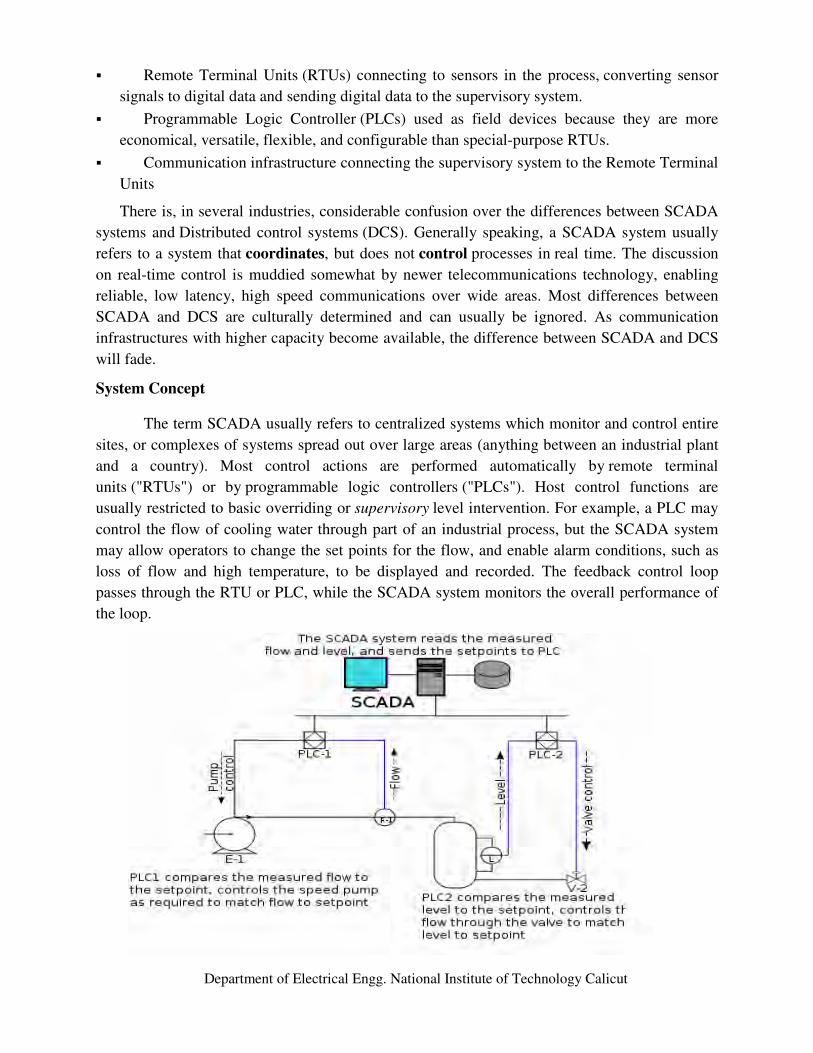
The term SCADA usually refers to centralized systems which monitor and control entire
sites, or complexes of systems spread out over large areas (anything between an industrial plant
and a country). Most control actions are performed automatically by remote terminal
units ("RTUs") or by programmable logic controllers ("PLCs"). Host control functions are
usually restricted to basic overriding or supervisory level intervention. For example, a PLC may
control the flow of cooling water through part of an industrial process, but the SCADA system
may allow operators to change the set points for the flow, and enable alarm conditions, such as
loss of flow and high temperature, to be displayed and recorded. The feedback control loop
passes through the RTU or PLC, while the SCADA system monitors the overall performance of
the loop.
Department of Electrical Engg. National Institute of Technology Calicut
Data acquisition begins at the RTU or PLC level and includes meter readings and
equipment status reports that are communicated to SCADA as required. Data is then compiled
and formatted in such a way that a control room operator using the HMI can make supervisory
decisions to adjust or override normal RTU (PLC) controls. Data may also be fed to a Historian,
often built on a commodity Database Management System, to allow trending and other analytical
auditing.
SCADA systems typically implement a distributed database, commonly referred to as
a tag database, which contains data elements called tags or points. A point represents a single
input or output value monitored or controlled by the system. Points can be either "hard" or "soft".
A hard point represents an actual input or output within the system, while a soft point results
from logic and math operations applied to other points. (Most implementations conceptually
remove the distinction by making every property a "soft" point expression, which may, in the
simplest case, equal a single hard point.) Points are normally stored as value-timestamp pairs: a
value, and the timestamp when it was recorded or calculated. A series of value-timestamp pairs
gives the history of that point. It's also common to store additional data with tags, such as the
path to a field device or PLC register, design time comments, and alarm information.
Substation Automation with SCADA
The substation SCADA system provides a common interface for various types of
equipments/devices used in the substation. Display & Database tools are used to configure the
interfaces used for controlling & monitoring the different equipment and the settings required for
protection, regulation or loading limits. The usage of alarm management systems prompts
various warning tags, control interlock logics relating to the current/past operations. The
graphical screens provide current information on all critical parameters. All the equipments can
be controlled & monitored through a single computer. Parameters such as actual & reactive
power, Energy, transformer temperature, Tap positions, Voltage, Current, Frequency, Power
factor, relay status & protection settings etc are collected and displayed in a user friendly
graphical format.
Substation automation can give adequate self checking, diagnostic features which helps
in providing proactive measures to establish a healthy system. The functions like Voltage
regulation, load management are implemented in substation software which reduces the usage of
complex components.
SCADA Lab Setup
The SCADA lab setup comprises of the following
Transmission Model (400/220 kV)
1. Panel 1: Station Model (415 V/110 V 3Φ transformer 1 KVA, Protection Relay Class-
1, 3Φ Energy Meters , PLC )
2. Panel 2: Transmission Line Model ( Resistors, Inductors & Capacitors), Series
compensators

Department of Electrical Engg. National Institute of Technology Calicut
3. Panel 3: Load Model for Transmission Line ( Dimmer, Resistors & Inductors) Shunt
Compensators, 3Φ Energy Meter
Distribution Model (11 kV)
4. Panel 4: Distribution Model (415 V/110 V 1Φ transformer 1 KVA, Protection Relay
Class-1, 3Φ Energy Meters , PLC, Dimmers, Resistors, Inductors & Capacitors)
The system consists of 400/220 kV transmission model & 11kV distribution substation
model, metering, protection and control devices, and a multi-tier SCADA system with scalable
distributed architecture. The proposed solution is based on the latest international standards in
substation communication and automation such as IEC 61850 and IEC 60870-5. The module
consists of RTU, protection relay, circuit breakers and energy meter for control, protection and
metering functions. PC based SCADA server/workstation is provided for local operation, data
logging, metering and sequence of events. The substation automation system is built on IEC
61850 open standard communication architecture. The software supplied is flexible and
compatible with above system to control entire substation modules and interfaces, simulate
power system distribution and network with single line diagrams. The SCADA software
monitors, communicates and operate RTUs, breakers and relays. Display for KWH, KVA, V, I,
Hz, Pf and kVAR is provided. The Control center consists of remote SCADA system for
operation, training & monitoring of the electrical network. The system communicates with
Transmission model in IEC 870-5-101 standard protocol.
Transmission Line Model
1) The model consists of 400/220 kV receiving substation with a 220 kV out going line.
2) One typical 220 kV transmission line also is modeled for a distance of 200 km.
3) The Communication System is built on the newest substation Communication
Architecture of IEC 61850.
Load Model
(R,L &C Load)
200 KM
Transmission Line Model
(8 pi Sections each of 25 km)
400/220 kV SS

Department of Electrical Engg. National Institute of Technology Calicut
Single Line
Diagram
Fuse
VM AM
Relay
1
Prot
CT 1/1 A
Metering
CT 1/1
Auxiliary Sup
ply
400/11
0 V
500 VA
, 1-Ph
3-Ph
Supply
Breaker
4 pole 32 A
C4C3C2C1
L, 1 kVA
R, 0.33 kV
AR/Ph,
5 A, 38.5 mH/
Ph
Contactor 1
10 V
4 pole 32 A
Contactor 1
10 V
4 pole, 32 A
R, 1 kW, 0
.33 kW
/Ph
5 A, 110
V
12.1 Ohm
/Ph
Load
Mod
el
3 ph
, 4 W
ire
12 ohm
Dimmer
3 ph
, 4 W
ire
12 oh
m Dimmer
Metering
CT 2.5/1 A
VM
Faul
t Thr
ow
Switc
hEM
1
C10
C4 C5
Capa
citor
Ban
k0.1
KVA
/Ph
0.3 K
VA/3-
Ph10
Nos
.
EM 1
AM VM
Metering
CT 2.5/1 A
MCB
32 A
400/
220
kV
Subs
tation
Mod
el
C2
VM AM
Metering
CT 2.5/1 A
C3Tr
ansm
ission
Line
8-Pi
secti
ons
220
kV, 2
00 K
MTr
ansm
ission
Lin
e M
odel
C6
C1
Serie
s
Compensation
415/110 V
1 KV
A, 12.5%
EM 2
EM 3
Department of Electrical Engg. National Institute of Technology Calicut
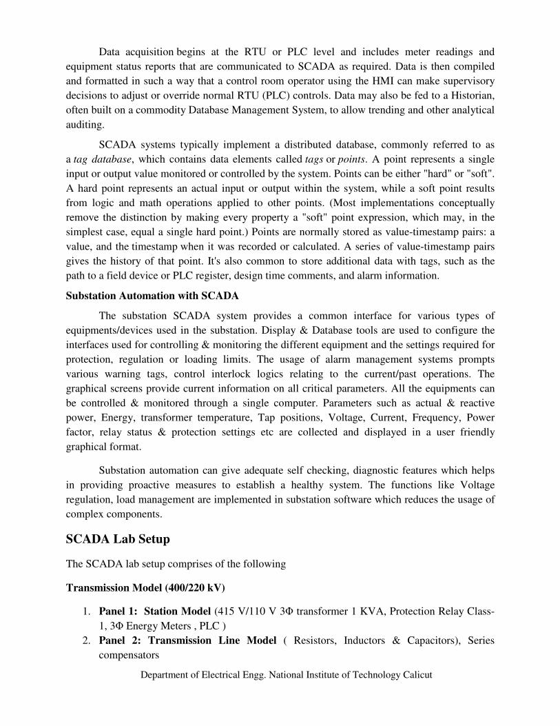
Communication Architecture
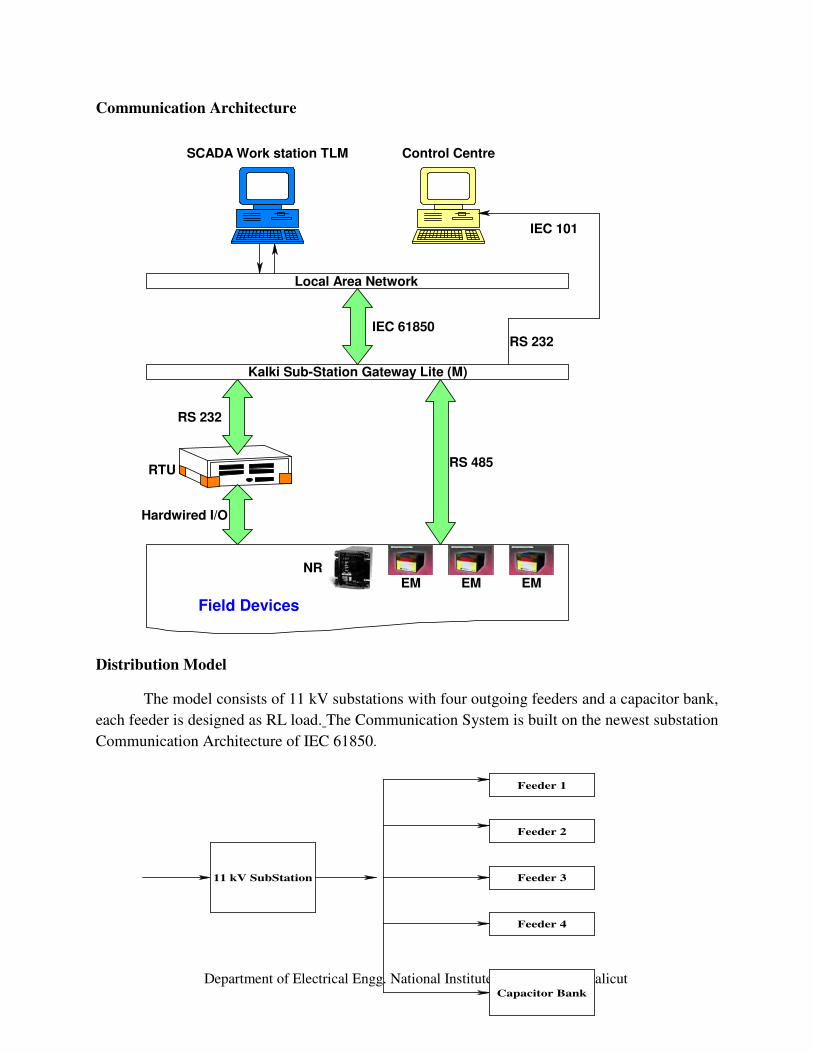
Distribution Model
The model consists of 11 kV substations with four outgoing feeders and a capacitor bank,
each feeder is designed as RL load. The Communication System is built on the newest substation
Communication Architecture of IEC 61850.
Kalki Sub-Station Gateway Lite (M)
Local Area Network
SCADA Work station TLM Control Centre
EM EM EMNR
Field Devices
IEC 61850
RS 485
IEC 101
RS 232
Hardwired I/O
RS 232
RTU
11 kV SubStation
Feeder 2
Feeder 1
Feeder 4
Feeder 3
Capacitor Bank

Department of Electrical Engg. National Institute of Technology Calicut
Single Line Diagram
16 A
Fuse1-Ph
Supply
MCB
1-Ph
16 A
C1
16 A
16 A
16 A
Capacitor Bank0.5 KVAR
1-Ph, LT, 5 Nos.
Prot CT
10/1
Metr CT
10/1
Feeder 1
Feeder 2
Feeder 3
Feeder 4
L, 4 taps230 V, 50 Ohm
L, 4 taps230 V, 50 Ohm
R 1KW230 V, 52.9 Ohm
R, 1 KW230 V, 52.9 Ohm
R, 1 KW230 V, 52.9 Ohm
R, 1 KW230 V, 52.9 Ohm
L, 4 taps230 V, 50 Ohm
L, 4 taps230 V, 50 Ohm
Prot CT
25/1 A
Metr CT
25/1 A
Metr CT
5/1 A
Metr CT
5/1 A
Metr CT
5/1 A
AM
AM
AM
AM
16 A
16 A
16 A
16 A
16 A
C3
C4
C6
C4
16 A
415/230 V, 1:1
5 KVA, 1-Ph, 5%
32 A
Metr CT
5/1 A
EM
EM
EM
EM
Relay
VM
AM
EM
C7
C8
C9
C10
C11
C2
Relay
EM
VM
AM
11 KV Distribution Model

Department of Electrical Engg. National Institute of Technology Calicut
EXPERIMENTS ON TRANSMISSION MODULE
Experiment Setup - Transmission Module
Precautions:
1. Once an experiment is selected in the SCADA system until it is completed and stopped
by clicking the stop button we shouldn’t click the main screen.
2. While closing the Circuit breaker make sure that the status of the breaker icon is updated
before going to close the next breaker (Vertical line on the breaker will be changed to
horizontal line)
3. Whenever a question mark (?) appears on the breaker icons, wait till the status is updated
without disturbing it, because it’s the problem of communication.
4. Always click the STOP button before going to the next experiment
Fuse
Relay 1
3-Ph Supply
Breaker4 pole 32 A
C4
C3
C2
C1
L, 1 kVAR, 0.33 kVAR/Ph,5 A, 38.5 mH/Ph
Contactor 110 V4 pole 32 A
Contactor 110 V4 pole, 32 A
R, 1 kW, 0.33 kW/Ph5 A, 110 V
12.1 Ohm/Ph
Load Model
3 ph, 4 Wire12 ohm Dimmer
3 ph, 4 Wire12 ohm Dimmer
Fault ThrowSwitch
EM 1
C10
Capacitor Bank0.1 KVA/Ph
0.3 KVA/3-Ph10 Nos.
MCB
32 A
400/220 kV Substation Model
220 kV, 200 KMTransmission Line
Model
C1
Series Compensation
415/110 V1 KVA, 12.5%
EM 2
EM 3
Prot CT 2.5/1 A
MeteringCT 2.5/1
Metering CT 5/1 A
MeteringCT 5/1 A
C2 C3 IN
R
X
CBM
Auxiliary Supply415/110 V500 VA, 1-Ph
Transmission Line8-Pi sections

Department of Electrical Engg. National Institute of Technology Calicut
Experiments overview – Transmission Model
The following experiments can be done using the Transmission Model both in Local and Remote
mode.
1. Fault Test
a. Line to Line Faults (LL)
b. Line to Ground Faults (LG)
c. Line to Line to Line Fault (LLL)
d. Line to Line to Ground Faults (LLG)
2. Ferranti Effect
3. Transmission Line Loading
a. Resistive Loading (R Load)
b. Inductive Loading (L load)
c. Resistive & inductive Loading (R & L Load)
4. Transformer Loading
a. Resistive Loading (R Load)
b. Inductive Loading (I load)
c. Resistive & Inductive Loading (R & L Load)
5. VAR Compensation
a. Shunt Compensation
b. Series compensation
i. Mid Point Compensation
ii. Sending End Compensation
iii. Receiving End Compensation
6. Operation of OLTC (Tap changing of transformer)
7. Sudden Load rejection
Common Procedure to All Experiments
1. Assemble S/S panel, Station Model, Transmission model & Load model.
2. Keep the Local/Remote selector in proper Position.
3. Keep all the Emergency Push buttons in released condition.
4. In the station model connect the energy meter & relay through the cables provided to the

Department of Electrical Engg. National Institute of Technology Calicut
corresponding pins.
5. Interconnect Station model & Transmission model using power cable
6. In the transmission model Connect the 3 Phase supply (R-Y-B) to the corresponding Input
pins of pin no. 4(4th pie section) & connect the O/p of 4th Pie to 5th pie & so on up to 8th Pie
O/p to the end pins of the pie section using cables provided. (Note: Phase lines should not be
interchanged)
7. Connect the transmission model & load Model using the power cable.
8. Change the phase current setting of the relay based on the load
9. Switch on the SCADA system & enter your login ID
10. Click ON the experiments screen

Department of Electrical Engg. National Institute of Technology Calicut
Local Mode Experiments
Exp No: Simulation of Faults (Local mode) Date:
L-G Fault
Aim:
Relay sensing and tripping and observe the fault current
Procedure:
1. Close the Incomer C1 by pressing the ON push button.
2. Configure the relay for the earth current settings, time multiplier for earth current & curve
number
3. Close the Breaker C2 by pressing the ON push button.
4. Close the Breaker C3 by clicking the Breaker icon in the SLD & follow the instructions
5. Select the system for simulating fault in the particular distance (100th KM, 150th
KM, and
175th KM) by closing the contactors 100th
KM, 150th
KM, 175th
KM by pressing the
corresponding ON push button.
6. Create the particular fault ( R-G, Y-G, B-G) by pressing the ON push buttons of L1, L2, L3
and G
7. The relay will trip the Line depending on the phase current setting and the time setting set on
the relay.
8. Once the system is tripped reset the relay manually
9. Click the back button & select the test results
10. The test results will display the details regarding the fault current & Nature of fault
11. Repeat the experiment for various phase currents and the time settings in the relay
12. Note the Fault current, Voltage & time to trip for various settings
13. Plot the current vs. time graph
After completing the experiment please de-energize/open all the breakers by pressing the OFF
push button of the corresponding contactors.
Observations:
Result:
It is observed that relay tripping is based on the current setting and time multiplier setting. It took
different time for different current values.
Sl No Current (%) Time(sec) Voltage
1
2
3

Department of Electrical Engg. National Institute of Technology Calicut
L-L Fault
Aim:
Relay sensing and tripping and observe the fault current
Procedure:
1. Close the Incomer C1 by pressing the ON push button.
2. Configure the relay for the earth current settings, time multiplier for earth current & curve
number
3. Close the Breaker C2 by pressing the ON push button.
4. Close the Breaker C3 by clicking the Breaker icon in the SLD & follow the instructions
5. Select the system for simulating fault in the particular distance (100th KM, 150th
KM, and
175th KM) by closing the contactors 100th
KM, 150th
KM, 175th
KM by pressing the
corresponding ON push button.
6. Create the particular fault (R-Y, Y-B, R-B) by pressing the ON push buttons of L1, L2, L3
7. Click the experiments screen & select the L-L Fault button, Configure the system for the
particular distance (100th KM, 150th KM, 175th KM)
8. The relay will trip the Line depending on the time setting set on the relay
9. Once the system is tripped reset the relay manually
10. Click the back button & select the test results
11. The test results will display the details regarding the fault current & Nature of fault
12. Repeat the experiment for various time settings in the relay
13. Note the Fault current, Voltage & time to trip for various settings
14. Plot the current vs. time graph
After completing the experiment please de-energize/open all the breakers by pressing the OFF
push button of the corresponding contactors.
Observations:
Result:
It is observed that relay tripping is based on the current setting and time multiplier setting. It took
different time for different current values.
Sl No Current (%) Time(sec) Voltage
1
2
3

Department of Electrical Engg. National Institute of Technology Calicut
L-L-L Fault
Aim:
Relay sensing and tripping and observe the fault current
Procedure:
1. Close the Incomer C1 by pressing the ON push button.
2. Configure the relay for the earth current settings, time multiplier for earth current & curve
number
3. Close the Breaker C2 by pressing the ON push button.
4. Close the Breaker C3 by clicking the Breaker icon in the SLD & follow the instructions
5. Select the system for simulating fault in the particular distance (100th KM, 150th
KM, and
175th KM) by closing the contactors 100th
KM, 150th
KM, 175th
KM by pressing the
corresponding ON push button.
6. Create the particular fault (R-Y, Y-B, R-B) by pressing the ON push buttons of L1, L2, L3
7. Click the experiments screen & select the L-L Fault button, Configure the system for the
particular distance (100th KM, 150th KM, 175th KM)
8. The relay will trip the Line depending on the time setting set on the relay
9. Once the system is tripped reset the relay manually
10. Click the back button & select the test results
11. The test results will display the details regarding the fault current & Nature of fault
12. Repeat the experiment for various time settings in the relay
13. Note the Fault current, Voltage & time to trip for various settings
14. Plot the current vs. time graph
After completing the experiment please de-energize/open all the breakers by pressing the OFF
push button of the corresponding contactors.
Observations:
Result:
It is observed that relay tripping is based on the current setting and time multiplier setting. It took
different time for different current values.
Sl No Current (%) Time(sec) Voltage
1
2
3

Department of Electrical Engg. National Institute of Technology Calicut
L-L-G Fault
Aim:
Relay sensing and tripping and observe the fault current
Procedure:
1. Close the Incomer C1 by pressing the ON push button.
2. Configure the relay for the earth current settings, time multiplier for earth current & curve
number
3. Close the Breaker C2 by pressing the ON push button.
4. Close the Breaker C3 by clicking the Breaker icon in the SLD & follow the instructions
5. Select the system for simulating fault in the particular distance (100th KM, 150th
KM, and
175th KM) by closing the contactors 100th
KM, 150th
KM, 175th
KM by pressing the
corresponding ON push button.
6. Create the particular fault (R-Y, Y-B, R-B) by pressing the ON push buttons of L1, L2, L3
and G
7. Click the experiments screen & select the L-L Fault button, Configure the system for the
particular distance (100th KM, 150th KM, 175th KM)
8. The relay will trip the Line depending on the time setting set on the relay
9. Once the system is tripped reset the relay manually
10. Click the back button & select the test results
11. The test results will display the details regarding the fault current & Nature of fault
12. Repeat the experiment for various time settings in the relay
13. Note the Fault current, Voltage & time to trip for various settings
14. Plot the current vs. time graph
After completing the experiment please de-energize/open all the breakers by pressing the OFF
push button of the corresponding contactors.
Observations:
Result:
It is observed that relay tripping is based on the current setting and time multiplier setting. It took
different time for different current values.
Sl No Current (%) Time(sec) Voltage
1
2
3

Department of Electrical Engg. National Institute of Technology Calicut
L-L-L-G Fault
Aim:
Relay sensing and tripping and observe the fault current
Procedure:
1. Close the Incomer C1 by pressing the ON push button.
2. Configure the relay for the earth current settings, time multiplier for earth current & curve
number
3. Close the Breaker C2 by pressing the ON push button.
4. Close the Breaker C3 by clicking the Breaker icon in the SLD & follow the instructions
5. Select the system for simulating fault in the particular distance (100th KM, 150th
KM, and
175th KM) by closing the contactors 100th
KM, 150th
KM, 175th
KM by pressing the
corresponding ON push button.
6. Create the particular fault (R-Y, Y-B, R-B) by pressing the ON push buttons of L1, L2, L3
and G
7. Click the experiments screen & select the L-L Fault button, Configure the system for the
particular distance (100th KM, 150th KM, 175th KM)
8. The relay will trip the Line depending on the time setting set on the relay
9. Once the system is tripped reset the relay manually
10. Click the back button & select the test results
11. The test results will display the details regarding the fault current & Nature of fault
12. Repeat the experiment for various time settings in the relay
13. Note the Fault current, Voltage & time to trip for various settings
14. Plot the current vs. time graph
After completing the experiment please de-energize/open all the breakers by pressing the OFF
push button of the corresponding contactors.
Observations:
Result:
It is observed that relay tripping is based on the current setting and time multiplier setting. It took
different time for different current values.
Sl No Current (%) Time(sec) Voltage
1
2
3

Department of Electrical Engg. National Institute of Technology Calicut
Exp No: Ferranti Effect (Local mode) Date:
Aim:
Simulating Ferranti effect in SCADA setup and observe the results
Procedure:
1. Close the Incomer C1 by pressing the ON push button
2. Close the Breaker C2 by pressing the ON push button
3. Close the Breaker C3 incomer for transmission line model by pressing the ON push button
4. Close the Breaker C3 for load model by pressing the ON push button
5. Check the Energy meter voltage of Energy meter 2 & Energy Meter 3.
6. Observe the Voltage at receiving end (EM3) and sending end (EM2) of the transmission line.
7. After completing the experiment please de-energize/open all the breakers by pressing the
OFF push button of the corresponding contactors.
Observations:
Sl No. Description Energy Meter 2 Energy Meter 3
Voltage (V) 1
Current (A)
Voltage (V) 2
Current (A)
Voltage (V) 3
Current (A)
Result:
Ferranti effect is observed in the experiment

Department of Electrical Engg. National Institute of Technology Calicut
Exp No: Transmission Line Loading (Local mode) Date:
Resistive Loading
Aim:
Load the transmission line by a resistive load and observe voltage and current profile
Procedure:
1. Close the Incomer C1 by pressing the ON push button
2. Close the Breaker C2 by pressing the ON push button
3. Close the Breaker C3 for transmission line model by pressing the ON push button
4. Close the Breaker C3 of the load model by pressing the ON push button
5. Close the breaker R by pressing the ON push button of the variable resistance.
6. Increase the load by rotating the dimmer check the current value in the screen and in the
EM3 for the receiving end parameters.
7. Click the test results & note the values as shown in the tabular column
8. Repeat the experiment for various current values. (Max up to 3A)
9. After completing the experiment please de-energize/open all the breakers by pressing the
OFF push button of the corresponding contactors.
Observations:
Sl No. Description Sending end Measurements Receiving end Measurements
1 Voltage (V)
2 Current (A)
3 Power (W)
4 VAR
5 Power Factor
Result:
Resistive loading of transmission line for 200km is conducted and observed the voltage and
current profiles.

Department of Electrical Engg. National Institute of Technology Calicut
Inductive Loading
Aim:
Load the transmission line by an inductive load and observe voltage and current profile
Procedure:
1. Close the Incomer C1 by pressing the ON push button
2. Close the Breaker C2 by pressing the ON push button
3. Close the Breaker C3 for transmission line model by pressing the ON push button
4. Close the Breaker C3 of the load model by pressing the ON push button
5. Close the breaker X by pressing the ON push button of the variable Inductance.
6. Increase the load by rotating the dimmer for inductance & check the current value in the
screen for the receiving end energy meter
7. Click the test results & note the values as shown in the tabular column
8. Repeat the experiment for various current values. (Max up to 3 A)
9. After completing the experiment please de-energize/open all the breakers by pressing the
OFF push button of the corresponding contactors.
Observations:
Sl No. Description Sending end Measurements Receiving end Measurements
1 Voltage (V)
2 Current (A)
3 Power (W)
4 VAR
5 Power Factor
Result:
Inductive loading of transmission line for 200km is conducted and observed the voltage and
current profiles.

Department of Electrical Engg. National Institute of Technology Calicut
Resistive and Inductive Loading
Aim:
Load the transmission line by resistive and inductive loads and observe voltage and current
profile
Procedure:
1. Close the Incomer C1 by pressing the ON push button
2. Close the Breaker C2 by pressing the ON push button
3. Close the Breaker C3 for transmission line model by pressing the ON push button
4. Close the Breaker C3 of the load model by pressing the ON push button
5. Close the breaker R by pressing the ON push button of a variable Resistance.
6. Close the breaker X by pressing the ON push button of a variable Inductance
7. Increase the load by rotating the dimmer for inductance & resistance, check the current value
in the screen for the receiving end energy meter
8. Click the test results & note the values as shown in the tabular column
9. Repeat the experiment for various current values. (Max up to 3 A)
10. After completing the experiment please de-energize/open all the breakers by pressing the
OFF push button of the corresponding contactors.
Observations:
Sl No. Description Sending end Measurements Receiving end Measurements
1 Voltage (V)
2 Current (A)
3 Power (W)
4 VAR
5 Power Factor
Result:
Resistive and inductive loading of transmission line for 200km is conducted and observed the
voltage and current profiles.

Department of Electrical Engg. National Institute of Technology Calicut
Exp No: Transformer Loading (Local mode) Date:
Resistive Loading
Aim:
Load the transformer by a resistive load and observe voltage and current profile
Procedure:
1. Close the Breaker C1 by pressing the ON push button
2. Close the Breaker C2 by pressing the ON push button
3. Close the Breaker C3 of the load model by pressing the ON push button
4. Close the breaker R by pressing the ON push button of the variable resistance
5. Increase the load by varying the dimmer positions, check the current value in the screen
for the receiving end energy meter
6. Click the test results & note the values as shown in the tabular column
7. Repeat the experiment for various current values. (Max up to 3 A)
8. After completing the experiment please de-energize/open all the breakers by pressing the
OFF push button of the corresponding contactors.
Observations:
Result:
Resistive loading of transformer is conducted and observed the voltage and current profiles.
Sl No. Description Incomer Measurements Sending end Measurements
1 Voltage (V)
2 Current (A)
3 Power (W)
4 VAR
5 Power Factor

Department of Electrical Engg. National Institute of Technology Calicut
Inductive Loading
Aim:
Load the transformer by an inductive load and observe voltage and current profile
Procedure:
1. Close the Breaker C1 by pressing the ON push button
2. Close the Breaker C2 by pressing the ON push button
3. Close the Breaker C3 of the load model by pressing the ON push button
4. Close the breaker X by pressing the ON push button of the variable Inductance
5. Increase the load by varying the dimmer positions, check the current value in the screen for the
receiving end energy meter
6. Click the test results & note the values as shown in the tabular column
7. Repeat the experiment for various current values. (Max up to 3 A)
8. After completing the experiment please de-energize/open all the breakers by pressing the
OFF push button of the corresponding contactors.
Observations:
Sl No. Description Incomer Measurements Sending end Measurements
1 Voltage (V)
2 Current (A)
3 Power (W)
4 VAR
5 Power Factor
Result:
Inductive loading of transformer is conducted and observed the voltage and current profiles.

Department of Electrical Engg. National Institute of Technology Calicut
Resistive and Inductive Loading
Aim:
Load the transmission line by resistive and inductive loads and observe voltage and current
profile
Procedure:
1. Close the Breaker C1 by pressing the ON push button
2. Close the Breaker C2 by pressing the ON push button
3. Close the Breaker C3 of the load model by pressing the ON push button
4. Close the breaker R by pressing the ON push button of the variable resistance.
5. Close the breaker X by pressing the ON push button of the variable Inductance
6. Increase the load by varying both the dimmer positions (resistance & inductance), check the
current value in the screen for the receiving end energy meter
7. Click the test results & note the values as shown in the tabular column
8. Repeat the experiment for various current values. (Max up to 3A at the receiving end)
9. After completing the experiment please de-energize/open all the breakers by pressing the
OFF push button of the corresponding contactors.
Observations:
Sl No. Description Incomer Measurements Sending end Measurements
1 Voltage (V)
2 Current (A)
3 Power (W)
4 VAR
5 Power Factor
Result:
Resistive and inductive loading of transformer is conducted and observed the voltage and current
profiles.

Department of Electrical Engg. National Institute of Technology Calicut
Exp No: VAR Compensation (Local mode) Date:
Series Compensation
Aim:
Study of series Var compensation at different points of transmission network and observe the
comparison
Procedure:
1. Close the Breaker C1 by pressing the ON push button
2. Close the Breaker C2 by pressing the ON push button
3. Close the Breaker C3 of the load model by pressing the ON push button
4. Close the breaker R by pressing the ON push button of the variable resistance.
5. Close the breaker X by pressing the ON push button of the variable Inductance
6. Increase the load by rotating the dimmer for inductance & resistance, check the current value
in the screen for the receiving end energy meter
7. Click the test results & note the values as shown in the tabular column
8. Open the Breaker C3 for Transmission line model by pressing the ON push button
For Sending End compensation
9. In the transmission model Connect the 3 Phase supply (R-Y-B) to the corresponding Input
pins I1, I2, I3 respectively & connect the O/p O1, O2, O3 to the input pins of the 1st pie
section using cables provided. (Note: Phase lines should not be interchanged)
For Receiving End compensation
10. In the transmission model Connect the 3 Phase supply (R-Y-B) to the corresponding Input
pins of 1st pie section & connect the O/p of 4th Pie to 5th Pie I/p & so on up to 8th Pie O/P.
Connect the 8th Pie O/p to input pins I1, I2, I3 respectively & connect the O/p O1, O2, O3 to
the 3 Phase output pins of the PI section using cables provided. (Note: Phase lines should not
be interchanged)
For Mid Point compensation
11. In the transmission model Connect the 3 Phase supply (R-Y-B) to the corresponding Input
pins of 1st PI section & connect the O/p of 4th Pie to input pins I1, I2, I3 respectively &
connect the O/p O1, O2, O3 to 5th Pie I/p and all other PI sections should be connected in
series & so on up to 8th Pie O/P & to the end pins of the pie section using cables provided.
(Note: Phase lines should not be interchanged)
12. Close the Breaker C3 of the transmission line model by pressing the ON push button.
13. Compare the values for different compensations without changing the load.
14. Click the test results & note the values as shown in the tabular column
15. After completing the experiment please de-energize/open all the breakers by pressing the
OFF push button of the corresponding contactors.

Department of Electrical Engg. National Institute of Technology Calicut
Observations:
Before
Compensation
Sending end
Compensation
Mid point
Compensation
Receiving
End compensation
S
No.
Description
Sending Receiving Sending Receiving Sending Receiving Sending Receiving
1 Voltage
(V)
2 Current
(A)
3 Power (W)
4 VAR
5 Power
Factor
Result:
Var compensation at different of transmission line is simulated and observed the voltage and
current profiles.

Department of Electrical Engg. National Institute of Technology Calicut
Shunt Compensation (Regulation of bus voltage)
Aim:
Study of shunt Var compensation at different points of transmission network and observe the bus
voltage.
Procedure:
1. Close the Breaker C1 by pressing the ON push button
2. Close the Breaker C2 by pressing the ON push button
3. Close the Breaker C3 of the load model by pressing the ON push button
4. Close the breaker R by pressing the ON push button of the variable resistance.
5. Close the breaker X by pressing the ON push button of the variable Inductance and vary
the corresponding dimmer so that the energy meter shows a lagging PF (i.e. 0.8 and less)
6. Close the breaker Capacitor Bank main of the capacitor bank main by pressing the ON
push button
7. Close the breakers CB1, CB2 in the branch carefully one by one until the power factor is
compensated for a value up to .99 lagging (i.e. unity power factor) (Note: Don’t close all
the capacitance breakers simultaneously as it will imbalance the complete system)
8. Click the test results & note the values as shown in the tabular column
9. After completing the experiment please de-energize/open all the breakers by pressing the
OFF push button of the corresponding contactors.
Observations:
Receiving end Measurements S No. Description
Before After
1 Voltage (V)
2 Current (A)
3 Power (W)
4 VAR
5 Power Factor
Result:
Shunt Var compensation is simulated in the system and bus voltage profile is observed

Department of Electrical Engg. National Institute of Technology Calicut
Exp No: Sudden Load Rejection (Local mode) Date:
Aim:
Apply the sudden load rejection to the transmission network and observe the voltage profiles.
Procedure:
1. Close the Breaker C1 by pressing the ON push button
2. Close the Breaker C2 by pressing the ON push button
3. Close the Breaker C3 of the load model by pressing the ON push button
4. Close the breaker R by pressing the ON push button of the variable resistance.
5. Close the breaker X by pressing the ON push button of the variable inductance.
6. Increase the load by varying the dimmer positions for inductance & resistance, check the
current value in the screen for the receiving end energy meter
7. Open the Breaker C3 by pressing the OFF push button.
8. Click the test results & note the values as shown in the tabular column
9. Repeat the experiment for various current values. (Max up to 2 A)
10. After completing the experiment please de-energize/open all the breakers by pressing the
OFF push button of the corresponding contactors.
Observations:
Receiving end Measurements S No. Description
Before c3 open After c3 open
Voltage (V) 1
Current (A)
Voltage (V) 2
Current (A)
Result:
Sudden load rejection is applied to the transmission network and the voltage profile is observed.

Department of Electrical Engg. National Institute of Technology Calicut
Remote Mode Experiments
Exp No: Simulation of Faults (Remote mode) Date:
L-G Fault
Aim:
Relay sensing and tripping and observe the fault current
Procedure:
1. Click the experiments screen & select the L-G Fault button, Configure the system for the
particular distance (100th KM, 150th
KM, 175th
KM)
2. Click the back button after configuring & go to the main screen
3. Close the Incomer C1 by clicking the Breaker icon in the SLD & follow the instructions
4. Configure the relay for the earth current settings, time multiplier for earth current & curve
number
5. Close the Breaker C2 by clicking the Breaker icon in the SLD & follow the instructions
6. Close the Breaker P2 by clicking the Breaker icon in the SLD & follow the instructions
7. Click on the Pie section in SLD screen
8. A screen showing the connections of Pie section will appear, Click the create fault screen
9. Select the particular fault (R-G, Y-G, B-G) by clicking the radio button & click apply
10. The relay will trip the Line depending on the phase current setting and the time setting set on
the relay.
11. Once the system is tripped reset the relay manually
12. Click the back button & select the test results
13. The test results will display the details regarding the fault current & Nature of fault
14. Repeat the experiment for various phase currents and the time settings in the relay
Observations:
Result:
It is observed that relay tripping is based on the current setting and time multiplier setting. It took
different time for different current values.
Sl No Current (%) Time(sec) Voltage
1
2
3

Department of Electrical Engg. National Institute of Technology Calicut
L-L Fault
Aim:
Relay sensing and tripping and observe the fault current
Procedure:
1. Click the experiments screen & select the L-L Fault button, Configure the system for the
particular distance (100th KM, 150th KM, 175th KM)
2. Click the back button after configuring & go to the main screen
3. Close the Incomer C1 by clicking the Breaker icon in the SLD & follow the instructions
4. Configure the relay for the Phase current settings, time multiplier for Phase current & curve
number
5. Close the Breaker C2 by clicking the Breaker icon in the SLD & follow the instructions
6. Close the Breaker P2 by clicking the Breaker icon in the SLD & follow the instructions
7. Click on the Pie section in SLD screen
8. A screen showing the connections of Pie section will appear, Click the create fault screen
9. Select the particular fault (R-Y, Y-B, R-B) by clicking the radio button & click apply
10. The relay will trip the Line depending on the time setting set on the relay
11. Once the system is tripped reset the relay manually
12. Click the back button & select the test results
13. The test results will display the details regarding the fault current & Nature of fault
Observations:
Result:
It is observed that relay tripping is based on the current setting and time multiplier setting. It took
different time for different current values.
Sl No Current (%) Time(sec) Voltage
1
2
3

Department of Electrical Engg. National Institute of Technology Calicut
L-L-L Fault
Aim:
Relay sensing and tripping and observe the fault current
Procedure:
1. Click the experiments screen & select the L-L-L Fault button, Configure the system for the
particular distance (100th KM, 150th KM, 175th KM)
2. Click the back button after configuring & go to the main screen
3. Close the Incomer C1 by clicking the Breaker icon in the SLD & follow the instructions
4. Configure the relay for the earth current settings, time multiplier for Phase current & curve
number
5. Close the Breaker C2 by clicking the Breaker icon in the SLD & follow the instructions
6. Close the Breaker P2 by clicking the Breaker icon in the SLD & follow the instructions
7. Click on the Pie section in SLD screen
8. A screen showing the connections of Pie section will appear, Click the create fault screen
9. Select the particular fault (R-Y-B) by clicking the radio button & click apply
10. The relay will trip the Line depending on the time setting set on the relay
11. Once the system is tripped reset the relay manually
12. Click the back button & select the test results
13. The test results will display the details regarding the fault current & Nature of fault
14. Repeat the experiment for various time settings in the relay
15. Note the Fault current, Voltage & time to trip for various settings
16. Plot the current vs. time graph
17. After completing the experiment please click close button to close the experiment
Observations:
Result:
It is observed that relay tripping is based on the current setting and time multiplier setting. It took
different time for different current values.
Sl No Current (%) Time(sec) Voltage
1
2
3

Department of Electrical Engg. National Institute of Technology Calicut
L-L-G Fault
Aim:
Relay sensing and tripping and observe the fault current
Procedure:
1. Click the experiments screen & select the L-L-G Fault button, Configure the system for the
particular distance (100th KM, 150th KM, 175th KM)
2. Click the back button after configuring & go to the main screen
3. Close the Incomer C1 by clicking the Breaker icon in the SLD & follow the instructions
4. Configure the relay for the Phase current setting, time multiplier for Phase current, curve
number, Earth current setting, Time multiplier for earth current & curve number
5. Close the Breaker C2 by clicking the Breaker icon in the SLD & follow the instructions
6. Close the Breaker P2 by clicking the Breaker icon in the SLD & follow the instructions
7. Click on the Pie section in SLD screen
8. A screen showing the connections of Pie section will appear, Click the create fault screen
9. Select the particular fault (R-Y-G, Y-B-G, R-B-G) by clicking the radio button & click apply
10. The relay will trip the Line depending on the time setting set on the relay
11. Once the system is tripped reset the relay manually
12. Click the back button & select the test results
13. The test results will display the details regarding the fault current & Nature of fault
14. Note the Fault current, for various settings
Observations:
Result:
It is observed that relay tripping is based on the current setting and time multiplier setting. It took
different time for different current values.
Sl No Current (%) Time(sec) Voltage
1
2
3

Department of Electrical Engg. National Institute of Technology Calicut
Exp No: Ferranti Effect (Remote mode) Date:
Aim:
Simulating Ferranti effect in SCADA setup and observe the results
Procedure:
1. Click the experiments screen & select the Ferranti effect button
2. Click the back button after configuring & go to the main screen
3. Close the Incomer C1 by clicking the Breaker icon in the SLD & follow the instructions
4. Close the Breaker C2 by clicking the Breaker icon in the SLD & follow the instructions
5. Close the Breaker P2 for panel 2 by clicking the Breaker icon in the SLD & follow the
instructions
6. Close the Breaker C3 by clicking the Breaker icon in the SLD & follow the instructions
7. Check the Energy meter voltage of Energy meter 2 & Energy Meter 3.
8. Observe the Voltage at receiving end (EM3) and sending end (EM2) of the transmission line.
Observations:
Sl No. Description Energy Meter 2 Energy Meter 3
Voltage (V) 1
Current (A)
Voltage (V) 2
Current (A)
Voltage (V) 3
Current (A)
Result:
Ferranti effect is observed in the experiment

Department of Electrical Engg. National Institute of Technology Calicut
Exp No: Transmission Line Loading (Remote mode) Date:
Resistive Loading
Aim:
Load the transmission line by a resistive load and observe voltage and current profile
Procedure:
1. Click the experiments screen & select the Transmission line loading button & select the
resistive load button
2. Click the back button after configuring & go to the main screen
3. Close the Incomer C1 by clicking the Breaker icon in the SLD & follow the instructions
4. Close the Breaker C2 by clicking the Breaker icon in the SLD & follow the instructions
5. Close the Breaker P2 for panel 2 by clicking the Breaker icon in the SLD & follow the
instructions
6. Close the Breaker C3 of the load model by clicking the Breaker icon in the SLD & follow the
instructions
7. Close the breaker C4 in the SLD which shows a variable resistance.
8. Increase the load by rotating the dimmer check the current value in the screen for the
receiving end energy meter
9. Click the test results & note the values as shown in the tabular column
10. Repeat the experiment for various current values.
Observations:
Sl No. Description Sending end Measurements Receiving end Measurements
1 Voltage (V)
2 Current (A)
3 Power (W)
4 VAR
5 Power Factor
Result:
Resistive loading of transmission line for 200km is conducted and observed the voltage and
current profiles.

Department of Electrical Engg. National Institute of Technology Calicut
Inductive Loading
Aim:
Load the transmission line by an inductive load and observe voltage and current profile
Procedure:
1. Click the experiments screen & select the Transmission line loading button & select the
inductive loading button
2. Click the back button after configuring & go to the main screen
3. Close the Incomer C1 by clicking the Breaker icon in the SLD & follow the instructions
4. Close the Breaker C2 by clicking the Breaker icon in the SLD & follow the instructions
5. Close the Breaker P2 for panel 2 by clicking the Breaker icon in the SLD & follow the
instructions
6. Close the Breaker C3 of the load model by clicking the Breaker icon in the SLD & follow the
instructions
7. Close the breaker C5 in the SLD, which shows a variable Inductance.
8. Increase the load by rotating the dimmer for inductance & check the current value in the
screen for the receiving end energy meter
9. Click the test results & note the values as shown in the tabular column
10. Repeat the experiment for various current values.
Observations:
Sl No. Description Sending end Measurements Receiving end Measurements
1 Voltage (V)
2 Current (A)
3 Power (W)
4 VAR
5 Power Factor
Result:
Inductive loading of transmission line for 200km is conducted and observed the voltage and
current profiles.

Department of Electrical Engg. National Institute of Technology Calicut
Resistive and Inductive Loading
Aim:
Load the transmission line by resistive and inductive loads and observe voltage and current
profile
Procedure:
1. Click the experiments screen & select the Transmission line loading button & select the R &
L button
2. Click the back button & after configuring go to the main screen
3. Close the Incomer C1 by clicking the Breaker icon in the SLD & follow the instructions
4. Close the Breaker C2 by clicking the Breaker icon in the SLD & follow the instructions
5. Close the Breaker P2 for panel 2 by clicking the Breaker icon in the SLD & follow the
instructions
6. Close the Breaker C3 by clicking the Breaker icon in the SLD & follow the instructions
7. Close the breaker C4 in the SLD, which shows a variable Resistance.
8. Close the breaker C5 in the SLD which shows a variable Inductance
9. Increase the load by rotating the dimmer for inductance & resistance, check the current value
in the screen for the receiving end energy meter
10. Click the test results & note the values as shown in the tabular column
11. Repeat the experiment for various current values. (Max up to 3 A)
Observations:
Sl No. Description Sending end Measurements Receiving end Measurements
1 Voltage (V)
2 Current (A)
3 Power (W)
4 VAR
5 Power Factor
Result:
Resistive and inductive loading of transmission line for 200km is conducted and observed the
voltage and current profiles.

Department of Electrical Engg. National Institute of Technology Calicut
Exp No: Transformer Loading (Remote mode) Date:
Resistive Loading
Aim:
Load the transformer by a resistive load and observe voltage and current profile
Procedure:
1. Click the experiments screen & select the Transformer loading button & select the R load
button
2. Click the back button & after configuring go to the main screen
3. Close the Incomer C1 by clicking the Breaker icon in the SLD & follow the instructions
4. Close the Breaker C2 by clicking the Breaker icon in the SLD & follow the instructions
5. Close the Breaker C3 of the load model by clicking the Breaker icon in the SLD & follow the
instructions
6. Close the breaker C4 in the SLD, which shows a variable Resistance.
7. Increase the load by varying the dimmer positions, check the current value in the screen for
the receiving end energy meter
8. Click the test results & note the values as shown in the tabular column
9. Repeat the experiment for various current values. (Max up to 3 A)
Observations:
Result:
Resistive loading of transformer is conducted and observed the voltage and current profiles.
Sl No. Description Incomer Measurements Sending end Measurements
1 Voltage (V)
2 Current (A)
3 Power (W)
4 VAR
5 Power Factor

Department of Electrical Engg. National Institute of Technology Calicut
Inductive Loading
Aim:
Load the transformer by an inductive load and observe voltage and current profile
Procedure:
1. Click the experiments screen & select the Transformer loading button & select the Inductive
load button
2. Click the back button & after configuring go to the main screen
3. Close the Incomer C1 by clicking the Breaker icon in the SLD & follow the instructions
4. Close the Breaker C2 by clicking the Breaker icon in the SLD & follow the instructions
5. Close the Breaker C3 of the load model by clicking the Breaker icon in the SLD & follow the
instructions
6. Close the breaker C5 in the SLD, which shows a variable inductance.
7. Increase the load by varying the dimmer positions, check the current value in the screen for
the receiving end energy meter
8. Click the test results & note the values as shown in the tabular column
9. Repeat the experiment for various current values.
Observations:
Sl No. Description Incomer Measurements Sending end Measurements
1 Voltage (V)
2 Current (A)
3 Power (W)
4 VAR
5 Power Factor
Result:
Inductive loading of transformer is conducted and observed the voltage and current profiles.

Department of Electrical Engg. National Institute of Technology Calicut
Resistive and Inductive Loading
Aim:
Load the transmission line by resistive and inductive loads and observe voltage and current
profile
Procedure:
1. Click the experiments screen & select the Transformer loading button & select the R & L
button
2. Click the back button & after configuring go to the main screen
3. Close the Incomer C1 by clicking the Breaker icon in the SLD & follow the instructions
4. Close the Breaker C2 by clicking the Breaker icon in the SLD & follow the instructions
5. Close the Breaker C3 of the load model by clicking the Breaker icon in the SLD & follow the
instructions
6. Close the breaker C4 in the SLD, which shows a variable resistance.
7. Close the breaker C5 in the SLD, which shows a variable inductance.
8. Increase the load by varying both the dimmer positions (resistance & inductance), check the
current value in the screen for the receiving end energy meter
9. Click the test results & note the values as shown in the tabular column
10. Repeat the experiment for various current values. (Max up to 3A at the receiving end)
Observations:
Sl No. Description Incomer Measurements Sending end Measurements
1 Voltage (V)
2 Current (A)
3 Power (W)
4 VAR
5 Power Factor
Result:
Resistive and inductive loading of transformer is conducted and observed the voltage and current
profiles.

Department of Electrical Engg. National Institute of Technology Calicut
Exp No: VAR Compensation (Remote mode) Date:
Series Compensation
Aim:
Study of series Var compensation at different points of transmission network and observe the
comparison
Procedure:
1. Click the experiments screen & select the VAR compensation button & select the Series
compensation
2. Click the back button & after configuring go to the main screen
3. Close the Incomer C1 by clicking the Breaker icon in the SLD & follow the instructions
4. Close the Breaker C2 by clicking the Breaker icon in the SLD & follow the instructions
5. Close the Breaker P2 for panel 2 by clicking the Breaker icon in the SLD & follow the
instructions
6. Close the Breaker C3 by clicking the Breaker icon in the SLD & follow the instructions
7. Close the breaker C4 in the SLD, which shows a variable Resistance.
8. Close the breaker C5 in the SLD which shows a variable Inductance
9. Increase the load by rotating the dimmer for inductance & resistance, check the current value
in the screen for the receiving end energy meter
10. Click the test results & note the values as shown in the tabular column
11. Open the Breaker P2 for panel 2 by clicking the Breaker icon in the SLD & follow the
instructions
For Sending End compensation
12. In the transmission model Connect the 3 Phase supply (R-Y-B) to the corresponding Input
pins I1, I2, I3 respectively & connect the O/p O1, O2, O3 to the input pins of the 1st pie
section using cables provided. (Note: Phase lines should not be interchanged)
For Receiving End compensation
13. In the transmission model Connect the 3 Phase supply (R-Y-B) to the corresponding Input
pins of 1st pie section & connect the O/p of 4th Pie to 5th Pie I/p & so on up to 8th Pie O/P.
Connect the 8th Pie O/p to input pins I1, I2, I3 respectively & connect the O/p O1, O2, O3 to
the 3 Phase output pins of the PI section using cables provided. (Note: Phase lines should not
be interchanged)
For Mid Point compensation
14. In the transmission model Connect the 3 Phase supply (R-Y-B) to the corresponding Input
pins of 1st PI section & connect the O/p of 4th Pie to input pins I1, I2, I3 respectively &
connect the O/p O1, O2, O3 to 5th Pie I/p and all other PI sections should be connected in
series & so on up to 8th Pie O/P & to the end pins of the pie section using cables provided.
(Note: Phase lines should not be interchanged)

Department of Electrical Engg. National Institute of Technology Calicut
15. Close the Breaker P2 by clicking the Breaker icon in the SLD & follow the instructions after
connecting the cables by selecting any of the compensations
16. Compare the values for different compensations with out changing the load.
17. Click the test results & note the values as shown in the tabular column
Observations:
Before
Compensation
Sending end
Compensation
Mid point
Compensation
Receiving
End compensation
S
No.
Description
Sending Receiving Sending Receiving Sending Receiving Sending Receiving
1 Voltage
(V)
2 Current
(A)
3 Power (W)
4 VAR
5 Power
Factor
Result:
Var compensation at different of transmission line is simulated and observed the voltage and
current profiles.

Department of Electrical Engg. National Institute of Technology Calicut
Shunt Compensation (Regulation of bus voltage)
Aim:
Study of shunt Var compensation at different points of transmission network and observe the bus
voltage.
Procedure:
1. Click the experiments screen & select the VAR Compensation button & select the Shunt
Compensation
2. Click the back button & after configuring go to the main screen
3. Close the Incomer C1 by clicking the Breaker icon in the SLD & follow the instructions
4. Close the Breaker C2 by clicking the Breaker icon in the SLD & follow the instructions
5. Close the Breaker P2 for panel 2 by clicking the Breaker icon in the SLD & follow the
instructions
6. Close the Breaker C3 by clicking the Breaker icon in the SLD & follow the instructions
7. Close the breaker C4 in the SLD, which shows a variable Resistance.
8. Close the breaker C5 in the SLD which shows a variable Inductance and vary the
corresponding dimmer so that the energy meter shows a lagging PF
9. Close the breaker C6 in the SLD which shows a mains capacitance branch with 10 breakers
10. Close the breakers in the branch carefully one by one until the power factor is compensated
for a value up to .99 lagging (ie. unity power factor) (Note: Don’t close all the capacitance
breakers simultaneously as it will imbalance the complete system)
11. Click the test results & note the values as shown in the tabular column
12. Repeat the experiment for various current values. (Max up to 3 A)
Observations:
Receiving end Measurements S No. Description
Before After
1 Voltage (V)
2 Current (A)
3 Power (W)
4 VAR
5 Power Factor
Result:
Shunt Var compensation is simulated in the system and bus voltage profile is observed

Department of Electrical Engg. National Institute of Technology Calicut
Exp No: Sudden Load Rejection (Remote mode) Date:
Aim:
Apply the sudden load rejection to the transmission network and observe the voltage profiles.
Procedure:
1. Click the experiments screen & select the Transmission line loading button & select the R &
L button
2. Click the back button & after configuring go to the main screen
3. Close the Incomer C1 by clicking the Breaker icon in the SLD & follow the instructions
4. Close the Breaker C2 by clicking the Breaker icon in the SLD & follow the instructions
5. Close the Breaker P2 for panel 2 by clicking the Breaker icon in the SLD & follow the
instructions
6. Close the Breaker C3 by clicking the Breaker icon in the SLD & follow the instructions
7. Close the breaker C4 in the SLD, which shows a variable Resistance.
8. Close the breaker C5 in the SLD which shows a variable Inductance
9. Increase the load by varying the dimmer positions for inductance & resistance, check the
current value in the screen for the receiving end energy meter
10. Open the Breaker C3 by clicking the Breaker icon in the SLD & follow the instructions
11. Click the test results & note the values as shown in the tabular column
12. Repeat the experiment for various current values. (Max up to 2 A)
Observations:
Receiving end Measurements S No. Description
Before c3 open After c3 open
Voltage (V) 1
Current (A)
Voltage (V) 2
Current (A)
Result:
Sudden load rejection is applied to the transmission network and the voltage profile is observed.

Department of Electrical Engg. National Institute of Technology Calicut
Exp No: Operation of OLTC Transformer (Remote mode) Date:
Aim:
Study the operation of OLTC transformer and observe the voltage regulation at sending end
Procedure:
1. Click the experiments screen & select the OLTC button
2. Click the back button & after configuring go to the main screen
3. Close the Incomer C1 by clicking the Breaker icon in the SLD & follow the instructions
4. Close the Breaker C2 by clicking the Breaker icon in the SLD & follow the instructions
5. Close the Breaker P2 for panel 2 by clicking the Breaker icon in the SLD & follow the
instructions
6. Close the Breaker C3 by clicking the Breaker icon in the SLD & follow the instructions
7. Close the breaker C4 in the SLD, which shows a variable Resistance.
8. Close the breaker C5 in the SLD which shows a variable Inductance
9. Increase the load by varying the dimmer positions for inductance & resistance, check the
current value in the screen for the receiving end energy meter
10. Once the load current is increased, the voltage will decrease then increase voltage by
changing the tap position of the transformer. Click the tap button above the transformer
symbol. A popup screen will appear, Raise the tap to increase the voltage/tap position or
lower it to reduce the voltage at lower loads
11. Click the test results & note the values as shown in the tabular column
Observations:
Sl.No. Tap position Sending end voltage (v)
1
2
3
4
5
Result:
Operation of OLTC transformer is studied and voltage regulation at the sending end is observed

Department of Electrical Engg. National Institute of Technology Calicut
EXPERIMENTS ON DISTRIBUTION MODULE
Experiment Setup - Distribution Module
Fuse1-Ph
Supply
MCB1-Ph
16 A
16 A
16 A
16 A
Feeder 1
Feeder 2
Feeder 3
Feeder 4
L, 4 taps230 V, 50 Ohm
L, 4 taps230 V, 50 Ohm
R 1KW230 V, 52.9 Ohm
R, 1 KW230 V, 52.9 Ohm
R, 1 KW230 V, 52.9 Ohm
R, 1 KW230 V, 52.9 Ohm
L, 4 taps230 V, 50 Ohm
L, 4 taps230 V, 50 Ohm
Prot CT
25/1 A
Metr CT
25/1 A
Metr CT
5/1 A
Metr CT
5/1 A
Metr CT
5/1 A
16 A
415/230 V, 1:1
5 KVA, 1-Ph, 5%
32 A
Metr CT
5/1 A
Relay
11 KV Distribution Model
EM
EM
EM
EM
EM
Capacitor Bank0.5 KVAR
1-Ph, LT, 5 Nos.
16 A
16 A
16 A
16 A
16 A
IN
F1
F2
F3
F4
CB1CB
CB2
CB3
CB4
CB5
Experiments overview- Distribution Model
The following experiments can be done using the Distribution Model
1. Relay Coordination
2. PF Control\Voltage Regulation
3. Transformer Loading
4. Demand side management
These experiments can be done in two modes i.e., Remote Mode and Local Mode.
Common Procedure to All Experiments:
1. Assemble Distribution Model.
2. Keep the Local/Remote selector in Local Position.
3. Keep the Emergency Push buttons in released condition.
4. Switch on the supply to the module by closing the MCB
5. Configure the Incomer relay for the current setting, time multiplier and curve number for
Phase current & Earth fault current

Department of Electrical Engg. National Institute of Technology Calicut
6. Configure the Feeder relay for the current setting, time multiplier and curve number for
Phase current & Earth fault current
7. Switch on the SCADA system & enter your login ID for observing the real Trends
8. Click the real trend icon on the main screen and select the parameters to observe with the
select pen option provided at the right side of the screen.
Precautions:
1. Once an experiment is selected in the SCADA system until it is completed and stopped
by clicking the stop button we shouldn’t click the main screen.
2. While closing the Circuit breaker make sure that the status of the breaker icon is updated
before going to close the next breaker (Vertical line on the breaker will be changed to
horizontal line)
3. Whenever a question mark (?) appears on the breaker icons, wait till the status is updated
without disturbing it, because it’s the problem of communication.
4. Always click the STOP button before going to the next experiment.

Department of Electrical Engg. National Institute of Technology Calicut
Local Mode Experiments
Exp No: Relay Co-ordination (Local mode) Date:
Aim:
Configure the protection relays to trip the circuit during overloading
Procedure:
1. Close the Sec contactor C1 (main incomer) by pressing the ON push button (Green)
2. Close the Feeder contactor F1 by pressing the ON push button.
3. Close the Feeder contactor F2 by pressing the ON push button.
4. Close the Feeder contactor F3 by pressing the ON push button.
5. Close the Feeder contactor F4 by pressing the ON push button.
6. Increase the load by varying the dimmer positions slowly for all the feeders & monitor the
load current in the energy meter as well as in the SCADA.
7. The relay will trip the Line depending on the time setting set on the relay & the overload.
8. The relay which have the lower current setting will trip first
9. The time settings can be synchronized in such a way that the feeder relay will pick up for
over load & the secondary relay will trip based on the overload condition
10. The test results will display the details regarding the fault current & Nature of fault
11. Repeat the experiment for various time settings in the relay
12. Note the Fault current, Voltage & time to trip for various settings
13. Plot the current vs. time graph
14. After completing the experiment please de-energize/open all the breakers by pressing the
OFF push button of the corresponding breakers provided on the module.
Observations:
Result:
Relay co-ordination is simulated and observed.
Sl No Current (%) Time(sec) Voltage
1
2
3

Department of Electrical Engg. National Institute of Technology Calicut
Exp No: PF Control/Voltage Regulation (Local mode) Date:
Aim:
Observe the voltage profile & PF at incomer and feeder side
Procedure:
1. Close the Sec contactor C1 (main incomer) by pressing the ON push button.
2. Close the Feeder contactor F1 by pressing the ON push button.
3. Close the Feeder contactor F2 by pressing the ON push button.
4. Close the Feeder contactor F3 by pressing the ON push button.
5. Close the Feeder contactor F4 by pressing the ON push button.
6. Increase the load by varying the dimmer positions slowly for all the feeders & monitor
the load current in the energy meter as well as in the SCADA.
7. Close the Capacitor Bank Contactor by pressing the ON push button of Capacitor bank
main
8. Note the PF & Voltage of the secondary side energy meter & the feeders
9. Close the Capacitor Bank branch Contactor one by one by pressing the ON push button
of CB1, CB2, CB3, CB4, and CB5. (Note: don’t switch on all the capacitor banks, check
the Pf profile accordingly switch on the capacitor banks based on the load)
10. The test results will display the details regarding Current, Voltage & PF
11. Repeat the experiment for various Load currents
12. Click the test results & note the values as shown in the tabular column
13. Repeat the experiment for various current values. (Max up to 3 A)
14. After completing the experiment please de-energize/open all the breakers by pressing the
OFF push button of the corresponding breakers.
Observations:
S
No.
Description Incomer
Measurements
Feeder (1,2,3,4)
Measurements
Remarks
1 Voltage (V)
2 Current (A)
3 Power (W)
4 VAR
5 Power Factor
6 VA
Result:
By using capacitor banks, pf can be adjusted and voltage regulation can be obtained.

Department of Electrical Engg. National Institute of Technology Calicut
Exp No: Transformer Loading (Local mode) Date:
Aim:
Load the transformer by increasing the feeder loads and observe voltage and current profile
Procedure:
1. Close the Sec contactor C1 by pressing the ON push button.
2. Close the Feeder contactor F1 by pressing the ON push button.
3. Close the Feeder contactor F2 by pressing the ON push button.
4. Close the Feeder contactor F3 by pressing the ON push button.
5. Close the Feeder contactor F4 by pressing the ON push button.
6. Increase the load by varying the dimmer positions slowly for all the feeders & monitor the
load current in the energy meter as well as in the SCADA.
7. Repeat the experiment for various Load currents
8. Click the test results & note the values as shown in the tabular column
9. Repeat the experiment for various current values. (Max up to 3 A)
10. After completing the experiment please de-energize/open all the breakers by pressing the
OFF push button of the corresponding breakers.
Observations:
S
No.
Description Incomer
Measurements
Feeder
Measurements
Remarks
1 Voltage (V)
2 Current (A)
3 Power (W)
4 VAR
5 Power Factor
6 VA
Result:
Transformer is loaded with the feeder and voltage and current profiles are observed.

Department of Electrical Engg. National Institute of Technology Calicut
Remote Mode Experiments
Exp No: Relay Co-ordination (Remote mode) Date:
Aim:
Configure the protection relays to trip the circuit during overloading
Procedure:
1. Click the experiments screen & select the Relay coordination, Configure the system
2. Click the back button after configuring & click the start button
3. Close the Sec contactor C1 by clicking the Breaker icon in the SLD & follow the instructions
4. Close the Feeder contactor C2 by clicking the Breaker icon in the SLD & follow the
instructions
5. Close the Feeder contactor C3 by clicking the Breaker icon in the SLD & follow the
instructions
6. Close the Feeder contactor C4 by clicking the Breaker icon in the SLD & follow the
instructions
7. Close the Feeder contactor C5 by clicking the Breaker icon in the SLD & follow the
instructions
8. Increase the load by varying the dimmer positions slowly for all the feeders & monitor the
load current in the energy meter.
9. The relay will trip the Line depending on the time setting set on the relay & the overload.
10. The relay which have the lower current setting will trip first
11. The time settings can be synchronized in such a way that the feeder relay will pick up for
over load & the secondary relay will trip based on the overload condition
12. The test results will display the details regarding the fault current & Nature of fault
13. Repeat the experiment for various time settings in the relay.
14. Note the Fault current, Voltage & time to trip for various settings
15. Plot the current vs. time graph
16. After completing the experiment, click close button to close the experiment
Observations:
Result:
Relay co-ordination is simulated and observed.
Sl No Current (%) Time(sec) Voltage
1
2
3

Department of Electrical Engg. National Institute of Technology Calicut
Exp No: PF Control/Voltage Regulation (Remote mode) Date:
Aim:
Observe the voltage profile & PF at incomer and feeder side
Procedure:
1. Click the experiments screen & select the PF\ Voltage Regulation, Configure the system
2. Click the back button after configuring & click the start button.
3. Close the Sec contactor C2 by clicking the Breaker icon in the SLD & follow the
instructions
4. Close the Feeder contactor C3 by clicking the Breaker icon in the SLD & follow the
instructions
5. Close the Feeder contactor C4 by clicking the Breaker icon in the SLD & follow the
instructions
6. Close the Feeder contactor C5 by clicking the Breaker icon in the SLD & follow the
instructions
7. Close the Feeder contactor C6 by clicking the Breaker icon in the SLD & follow the
instructions
8. Increase the load by varying the dimmer positions slowly for all the feeders & monitor
the load current in the energy meter
9. Close the Capacitor Bank Contactor by clicking the Breaker icon in the SLD & follow
the instructions
10. Note the PF & Voltage of the secondary side energy meter & the feeders
11. Close the Capacitor Bank branch Contactor one by one by clicking the Breaker icon in
the SLD & follow the instructions. The test results will display the details regarding
Current, Voltage & PF. Click the test
12. Repeat the experiment for various current values. (Max up to 3 A)
Observations:
S
No.
Description Incomer
Measurements
Feeder (1,2,3,4)
Measurements
Remarks
1 Voltage (V)
2 Current (A)
3 Power (W)
4 VAR
5 Power Factor
6 VA
Result:
By using capacitor banks, pf can be adjusted and voltage regulation can be obtained.

Department of Electrical Engg. National Institute of Technology Calicut
Exp No: Transformer Loading (Remote mode) Date:
Aim:
Load the transformer by increasing the feeder loads and observe voltage and current profile
Procedure:
1. Click the experiments screen & select the Transformer loading, Configure the system
2. Click the back button after configuring & click the start button.
3. Close the Sec contactor C1 by clicking the Breaker icon in the SLD & follow the instructions
4. Close the Feeder 1 contactor C2 by clicking the Breaker icon in the SLD & follow the
instructions
5. Close the Feeder 2 contactor C3 by clicking the Breaker icon in the SLD & follow the
instructions
6. Close the Feeder 3 contactor C4 by clicking the Breaker icon in the SLD & follow the
instructions
7. Close the Feeder 4 contactor C5 by clicking the Breaker icon in the SLD & follow the
instructions
8. Increase the load by varying the dimmer positions slowly for all the feeders & monitor the
load current in the energy meter
9. Repeat the experiment for various Load currents
10. Click the test results & note the values as shown in the tabular column
11. Repeat the experiment for various current values. (Max up to 3 A)
12. After completing the experiment please click close button to close the experiment
Observations:
S
No.
Description Incomer
Measurements
Feeder
Measurements
Remarks
1 Voltage (V)
2 Current (A)
3 Power (W)
4 VAR
5 Power Factor
6 VA
Result:
Transformer is loaded with the feeder and voltage and current profiles are observed.

Department of Electrical Engg. National Institute of Technology Calicut
Exp No: Demand Side Management (Remote mode) Date:
Aim:
Apply demand side management in the present system and observe the load management results
Procedure:
1. Click the experiments screen & select the Demand side Management (Load management),
Configure the system
2. In the configuration screen select the different priorities for different feeders (1- 4).
3. Click the back button after configuring & click the start button.
4. Close the Sec contactor C1 by clicking the Breaker icon in the SLD & follow the instructions
5. Close the Feeder 1 contactor C2 by clicking the Breaker icon in the SLD & follow the
instructions
6. Close the Feeder 2 contactor C3 by clicking the Breaker icon in the SLD & follow the
instructions
7. Close the Feeder 3 contactor C4 by clicking the Breaker icon in the SLD & follow the
instructions
8. Close the Feeder 4 contactor C5 by clicking the Breaker icon in the SLD & follow the
instructions
9. Rotate the dimmer slowly for all the feeders & monitor the load current in the energy meter
10. Once the load is increased greater than the secondary feeder the least priority feeder will trip
to compensate the overload.
11. Repeat the experiment for various Load currents
12. Click the test results & note the values as shown in the tabular column
13. Repeat the experiment for various current values. (Max up to 3 A)
14. After completing the experiment please click close button to close the experiment
Observations:
S
No.
Description Sending end
Measurements
Feeder
Measurements
Remarks
1 Voltage (V)
2 Current (A)
3 Power (W)
4 VAR
5 Power Factor
6 VA
Results:
Demand side load management strategy is observed.

Department of Electrical Engg. National Institute of Technology Calicut
Programmable Logic Controller Experiments
Introduction
The programmable logic controller (PLC) is a solid state electronic device designed in the
early 1970’s to replace electromechanical relays, timers, counters and sequences, which uses a
programmable memory for the internal storage of user oriented instructions for implementing
specific functions such as logic sequencing timing, country and arithmetic control through digital
or analog inputs and outputs, various types of machines or processes.
The introduction of microprocessor changed the PLC industry .PLC have been reduced in size,
processing power increased and PLCs are now capable at the most complex program
algorithms. Originally PLC s were programmed only in RLL, they can now be programmed in
several styles and types of programming languages such as SFC (sequential function chart), state
language, control block languages and statement languages such as BASIC. With the growth in
technology PLCs are now capable of advanced data manipulations, communications and process
controls. Benefits of using PLC in industries are
1. The PLC is a hardened industrial computer designed to withstand the harsh
factory environment.
2. PLSs is reusable they contain a changeable program that eliminators extensive
and component changes.
3. PLCs offer easy troubleshooting
4. PLCs feature easy installation and small size.
The PLC has the basic structure shown in figure. It has four main units.
1. The Programme Memory – The instructions for the logical control sequences are stored
here.
2. The Data Memory – The status of switches, interlocks, past values of data and other
working data is stored here.
3. The Output Device – These are hardware/software drivers for the industrial process
actuators, such as solenoids switches, motors and valves.
4. The Input Devices – These are hardware/software drivers for industrial process sensors
such as switch status sensors, proximity detectors. Interlocks settings and so on.
5. In addition to this the PLC has a programming unit. This is either a special module, a
PC connected to the PLC by the serial link, or both. The programming unit is used to
build, test and edit the logical sequence that the PLC will execute.
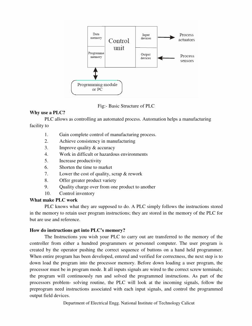
Department of Electrical Engg. National Institute of Technology Calicut
Fig:- Basic Structure of PLC
Why use a PLC?
PLC allows as controlling an automated process. Automation helps a manufacturing
facility to
1. Gain complete control of manufacturing process.
2. Achieve consistency in manufacturing
3. Improve quality & accuracy
4. Work in difficult or hazardous environments
5. Increase productivity
6. Shorten the time to market
7. Lower the cost of quality, scrap & rework
8. Offer greater product variety
9. Quality charge over from one product to another
10. Control inventory
What make PLC work
PLC knows what they are supposed to do. A PLC simply follows the instructions stored
in the memory to retain user program instructions; they are stored in the memory of the PLC for
but are use and reference.
How do instructions get into PLC’s memory?
The Instructions you wish your PLC to carry out are transferred to the memory of the
controller from either a hundred programmers or personnel computer. The user program is
created by the operator pushing the correct sequence of buttons on a hand held programmer.
When entire program has been developed, entered and verified for correctness, the next step is to
down load the program into the processor memory. Before down loading a user program, the
processor must be in program mode. It all inputs signals are wired to the correct screw terminals;
the program will continuously run and solved the programmed instructions. As part of the
processors problem- solving routine, the PLC will look at the incoming signals, follow the
preprogram need instructions associated with each input signals, and control the programmed
output field devices.

Department of Electrical Engg. National Institute of Technology Calicut
Some of the used Instructions
Bit Instructions
The following instructions are used with fixed, SLC 5/01, SLC 5/02, SLC 5/03, and SLC 5/04
processors.
If you want to: Use this Instruction:
Examine a bit for an On conditions XIC
Examine a bit for an Off conditions XIO
Turn a bit On or Off OTE
Turn a bit On OLT
Turn a bit Off OUT
Trigger a one time event OSR
Examine if Closed (XIC)
Use the XIC instruction in your ladder to determine if a bit is on. When the
instruction is executed, if the bit addressed is on (1), then the instruction is
evaluated as true. When the instruction is executed, if the bit addressed off (0),
then the instruction is evaluated as false.
Examine if Open (XIO)
Use an XIO instruction in your ladder program to determine if a bit is off. When
the instruction is executed, if the bit addressed is off (0), then the instruction is
evaluated as true. When the instruction is evaluated as false.
Output Energize
Use an OTE instruction in your ladder program to turn on a bit when rung
conditions are evaluated as true.
Output Latch (OTL)
The OTL instruction is a retentive output instruction that can only turn on a bit. It
cannot turn off a bit. This instruction is traditionally used in pairs with an Output
Unlatch (OUT) instruction, with both instructions addressing the same bit. You
can also use this to initialize data values at the bit level.
Output Unlatch (OTU)
The OTU instruction is a retentive output instruction that can only turn off a bit. If
cannot turn on a bit. This instruction is traditionally used in pairs with an Output
Latch (OTL) instruction, with both instructions addressing the same bit. You can
use this to initialize data values at the bit level.
] [
] [
( )
(L)
(U)

Department of Electrical Engg. National Institute of Technology Calicut
One Short Rising (OSR)
The OSR instruction is a retentive input instruction that triggers an event to occur
one time. Use the OSR instruction when an event must start based on the change
of state of the rung from false to true, not on the resulting status. Applications
include starting events triggered by a pushbutton switch. An example is freezing
rapidly displayed LED values.
Timer and Counter Instructions
Timers and counters are output instructions. Use the following instructions with fixed, SLC 5/01,
SLC 5/02, SLC 5/02, SLC 5/03, and SLC 5/04 processors.
If you want to: Use this instruction:
Count time base intervals when the instruction is true TON
Count time base intervals when the Instruction is false TOF
Count time base intervals when the instruction is true and
retain the accumulated value when the instruction
goes false
RTO
Increment the count at each false–to–true transition. CTU
Decrement the count at each false-to-true transition CTD
Count high-speed pulses from a fixed
Controller High-speed input HSE
Reset the accumulated value and status bits of a timer or
counter. Do not use with TOF timers. RES
Timer On-Delay (TON)
Use the TON instruction to turn an output on or off after the timer
has been on for a preset time interval. The TON instruction begins
to count time base intervals when rung conditions become true. As
long as rung conditions remain true, the timer adjusts its
accumulated value (ACC) each evaluation until it reaches the
preset value (PRE). The accumulated value is reset when rung
conditions go false, regardless of whether the timer has timed out.
Timer Off-Delay (TOF)
Use the TOF instruction to turn an output on or off after is rung has
been off for a preset time interval. The TOF instruction begins to
count time base intervals when the rung makes a true-to-false
transition. As long as rung conditions remain false, the timer
increments its accumulated value (ACC) each scan until it reaches
] OSR [
TON
TIMER ON DELAY
Timer T4: 0
Timer Base 0.01
TOF
TIMER OFF DELAY
Timer T4:1
Time base 0.01

Department of Electrical Engg. National Institute of Technology Calicut
the preset value (PRE). The accumulated value is reset when rung
conditions go true regardless of whether the timer has timed out.
Retentive Timer (RTO)
Use the RTO instruction to turn an output on or off after its timer
has been on for a preset time interval. The RTO instruction is a
retentive instruction that begins to count time base intervals when
rung conditions become true. As long as rung conditions remain
true, the timer increments its accumulated value (ACC) until it
reaches the preset value (PRE).
Using counters
Counter instructions have three word data file elements. Word 0 is the control word, containing
the status bits of the instructions. Word 1 is the preset value; word 2 is the accumulated value.
How Counters Work: The figure below demonstrates how a counter works. The count value
must remain in the range of –32768, a counter status overflow (OV) or underflow (UN) bit is set.
Count Up (CTU)
The CTU is a retentive output instruction that counts false-to-true
rung transitions. Rung transitions can be caused by events
occurring in the program such as parts traveling past a detector or
actuating a limit switch.
Count Down (CTD)
The CTD is a retentive output instruction that counts false-to-true
rung transitions Rung transitions can be caused by events
occurring in the program such as parts traveling past a detector or
actuating a limit switch.
High-Speed Counter (HSC)
The High-Speed Counter is a variation of the CTU counter. The
HSC instruction is enabled when the rung logic is true and disabled
when the rung logic is false.
RTO
RETENTIVE TIMER
ON
Timer T4: 2
Time base 0.01
CTU
COUNT UP
Counter C5:0
Preset 120
CTD
COUNT DOWN
Counter C5:1
Preset 120
HSC
HIGH SPEED
COUNTER
Counter
C5:0
Preset 120

Department of Electrical Engg. National Institute of Technology Calicut
Reset (RES)
Use a RES instruction to reset a timer or counter. When the RES
instruction is enabled, it resets the retentive on-delay timer, count
up, or countdown instruction having the same address as the RES
instruction.
Math Instruction
The following output instruction allows you to perform computation and math operations on
individual words. Use these instructions with fixed. SLC 5/01, SLC 5/02, SLC 5/03, and SLC
5/04 processors, except where noted.
If you want to: Use this instruction
Add two values ADD
Subtract two values SUB
Multiply one value from another MUL
Divide one value by another DIV
Perform a double divide DDV
Change the sign of the
source value and place it in the destination NEG
Set all bits of a world to zero CLR
Convert an integer to BCD TOD
Convert a BCD value to an integer value FRD
Multiplex data DCD
Find the square roof of a value SQR
Scale a value SCL
Add (ADD)
Use the ADD instruction to add one value (source A) to another value
(source B) and place the result in the destination.
Subtract (SUB)
Use the SUB instruction to subtract one value (Source B) from another
(Source A) and place the result in the destination.
ADD
Source A
Source B
Dest
SUB
Subtract
Source A
Source B
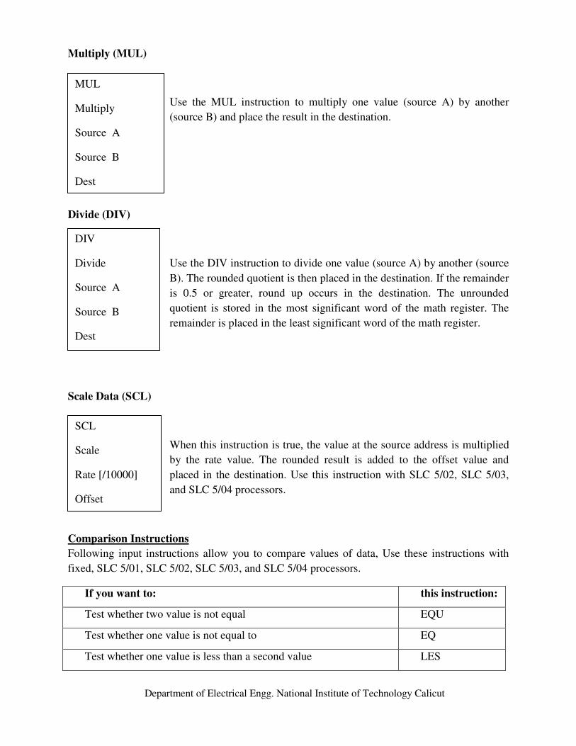
Department of Electrical Engg. National Institute of Technology Calicut
Multiply (MUL)
Use the MUL instruction to multiply one value (source A) by another
(source B) and place the result in the destination.
Divide (DIV)
Use the DIV instruction to divide one value (source A) by another (source
B). The rounded quotient is then placed in the destination. If the remainder
is 0.5 or greater, round up occurs in the destination. The unrounded
quotient is stored in the most significant word of the math register. The
remainder is placed in the least significant word of the math register.
Scale Data (SCL)
When this instruction is true, the value at the source address is multiplied
by the rate value. The rounded result is added to the offset value and
placed in the destination. Use this instruction with SLC 5/02, SLC 5/03,
and SLC 5/04 processors.
Comparison Instructions
Following input instructions allow you to compare values of data, Use these instructions with
fixed, SLC 5/01, SLC 5/02, SLC 5/03, and SLC 5/04 processors.
If you want to: this instruction:
Test whether two value is not equal EQU
Test whether one value is not equal to EQ
Test whether one value is less than a second value LES
MUL
Multiply
Source A
Source B
Dest
DIV
Divide
Source A
Source B
Dest
SCL
Scale
Rate [/10000]
Offset

Department of Electrical Engg. National Institute of Technology Calicut
Test whether one value is less than or equal to a second value LEQ
Test whether one equal to second value is greater than another GRT
Test whether one value is greater than or equal to a second value GEQ
Test portions of two values to see whether they are equal MEQ
Test whether one value is within the limit range of two other values LIM
Equal (EQU)
Use the EQU instruction to test whether two values are equal. If source
A and source B are equal, the instruction is logically true. If these
values are not equal, the instruction is logically false.
Not Equal (NEQ)
Use the NEQ instruction to test whether two values are not equal. If
source A and source B are not equal, the instruction is logically true. If
the two values are equal, the instruction is logically false.
Less Than (LES)
Use the LES instruction to test whether one value (source A) is less
than another (source B). If source A is less than the value at source B
the instruction is logically true. If the value at source A is greater than
or equal to the value at source B, the instruction is logically false.
Less Than or Equal (LEQ)
Use the LEQ instruction to test whether one value (source A) is less
than or equal to another (source B). If the value at source A is less
than or equal to the value at source B, the instruction is logically
EQU
EQUAL
Source A
Source B
NEQ
NOT EQUAL
Source A
Source B
LES
LESS THAN
Source A
Source B
LEQ
LESS THAN OR
EQUAL
Source A
Source B

Department of Electrical Engg. National Institute of Technology Calicut
true. If the value at source A is greater than the value at source B, the
instruction is logically false.
Greater Than (GRT)
Use the GRT instruction to test whether one value (source A) is
greater than another (source B). If the value at source A is greater
than the value at source B. The instruction is logically true. If the
value at source A is less than or equal to the value at source B, the
instruction is logically false.
Greater Than or Equal (GEQ)
Use the GEQ instruction to test whether one value (source A) is
greater than or equal to another (source B). If the value at source A is
greater than or equal to the value at source B, the instruction is
logically true. If the value at source A is less than the value at source
B, the instruction is logically false.
Masked Comparison for Equal MEQ)
Use the MEQ instruction to compare data at a source address with
data at a reference address. Use of this instruction allows portions of
the data to be masked by a separate word.
Limit Test (LIM)
Use the LIM instruction to test for value within or outside a specified
range, depending on how you set the limits. Use this instruction with
5/02 and 5/03 processors.
GRT
GREATER THAN
Source A
Source B
GEQ
GREATER THAN
OR EQUAL
Source A
Source B
MEQ
MASKED EQUAL
Source
Mask
Compare
LIM
LIMIT TEST
Test
High Lim
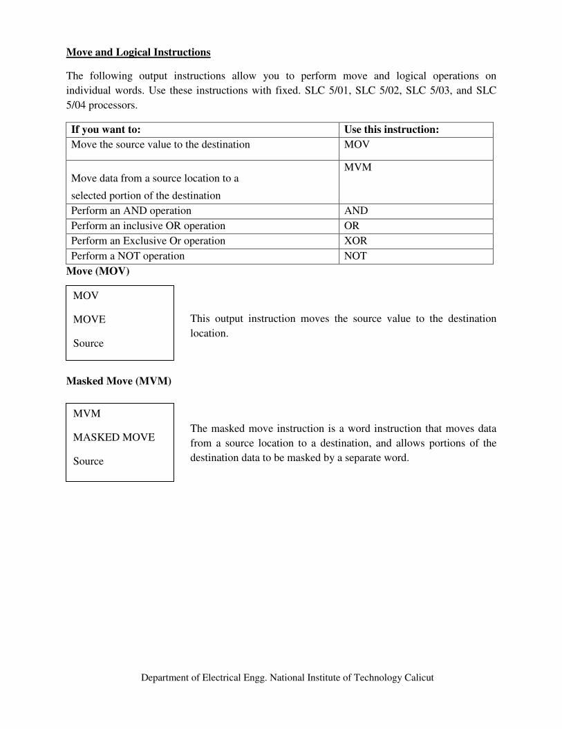
Department of Electrical Engg. National Institute of Technology Calicut
Move and Logical Instructions
The following output instructions allow you to perform move and logical operations on
individual words. Use these instructions with fixed. SLC 5/01, SLC 5/02, SLC 5/03, and SLC
5/04 processors.
If you want to: Use this instruction:
Move the source value to the destination MOV
Move data from a source location to a
selected portion of the destination
MVM
Perform an AND operation AND
Perform an inclusive OR operation OR
Perform an Exclusive Or operation XOR
Perform a NOT operation NOT
Move (MOV)
This output instruction moves the source value to the destination
location.
Masked Move (MVM)
The masked move instruction is a word instruction that moves data
from a source location to a destination, and allows portions of the
destination data to be masked by a separate word.
MOV
MOVE
Source
MVM
MASKED MOVE
Source

Department of Electrical Engg. National Institute of Technology Calicut
EXPERIMENTS
Exp No: SPEED CONTROL OF AC SERVO MOTOR Date:
Aim:
To control the speed of an AC servomotor by implementing pi controller using PLC ladder
logic program.
Theory:
Proportional Control
The controller is proportional; it will produce a control signal, which is proportional to
the input error signal, i.e., signal proportional to the difference between actual level and desired
level. When the error is high the controller will send the signal according the error. In the graph
we can see the same.
When it is in position control, the control signal is almost a straight line and has no
relation with error but in P- controller we can see that the controller output is varying according
the error.
Let the signal be u (t) which is proportional to the input error signal, e (t). Then we can
obtain a relation
U (t) = kpe (t)
Where Kp proportional gain (or) constant
U(s)
------ = Kp
E(s)
Hence, we can say that the proportional controller amplifies the error signal by an amount Kp.
Also the introduction of the controller on the system increases the loop gain by an amount Kp.
The increase in loop gain improves the steady state tracking accuracy, disturbance signal
rejection and the relative stability and also makes the system less sensitive to parameter
variations. But increasing the gain to very large values may lead to instability of the system. The
demerit of P- controller is that it leads to a constant steady state error.

Department of Electrical Engg. National Institute of Technology Calicut
Proportional + Integral Controller
The integral (or) reset action combine with proportional control gives us a controller
which will always act to maintain the control variable as its desired value (set point). The
proportional mode provides a stabilizing influence while the integral mode will help to overcome
the OFFSET. Integral controller will provide corrective action as long as there is a deviation in
the controlled variable from the set point value. Integral control has a phase lag of 900
proportional controls. This lagging feature of reset will result in a slow responses & oscillation
will come in to picture.
The proportional & integral controller produce an output signal consisting of 2-terms, one
is proportional to error signal & the other proportional to the integral of the error signal.
U(s) 1
We write -------- = Kp [ 1 + ----- ]
E(s) Ti S
The advantage of both P & I controller are combined in P-I controller, the proportional
action increased the loop gain & makes the system less sensitive to variations of system
parameters. The integral action eliminates (or) reduces the steady state error.
The integral action is adjusted by varying the integral time. The inverse of integral time
T is called the reset value.
Proportional + Integral + Derivative Control
When the all three control effects are combined together we obtain the benefits of each
control action & more over the effect duplicates the action of good human operator on a control
application. A three controller contains the stability of P- controller and the ability to eliminate
offset because of reset control and ability to provide an immediate corrective action for the
magnitude of a disturbance because of rate control.
Kp de(t)
µ(t) = µ0 + Kp e(t) + ------ ∫ e(t)dt + KPTD [ -------- ]
Ti dt
KD = KPTD

Department of Electrical Engg. National Institute of Technology Calicut
Apparatus required:
1. AC servomotor kit
2. PLC (Allen Bradley Micrologix 1500 LRP series C)
3. PC with Versapro Software
4. RS232 cable
5. Patch chords
Procedure:
1. Load the Versapro software to the PC
2. Open the Versapro software
3. Switch on the PLC trainer and lift controls system
4. Connect PLC with AC servomotor kit.
5. Open the New folder and draw the ladder logic program
6. Select the correct hardware configuration.
7. Store the Program to PLC
8. Run the program
9. Verify the performance to the control AC servomotor.
Description:
Applying different voltages can control speed of the AC servomotor. For this purpose AC
voltage controller has been used. Accordingly triggering angle control for this circuit has
accomplished by plc ladder logic program. For measurement of speed an optocoupler is used in
conjunction with a square geared wheel connected to the shaft of the motor. The optocoupler
measures speed of motor by noting the number of tooth that it encountered in a fixed time. The
optocoupler output is given to the analog input port of plc kit. Then control algorithm will
compare this value with the default set point value, which give an error signal. This error signal
is used in manipulating the firing angle of thyristor circuit to control applied voltage to the
servomotor. Ladder logic program also facilitates the user to tune the controller parameters to
change the performance of the controller and to set desired speed value.
Observations:
What do you infer from the controller output oscillations? By varying the proportional gain,
integral gain, what would be the merits and demerits?
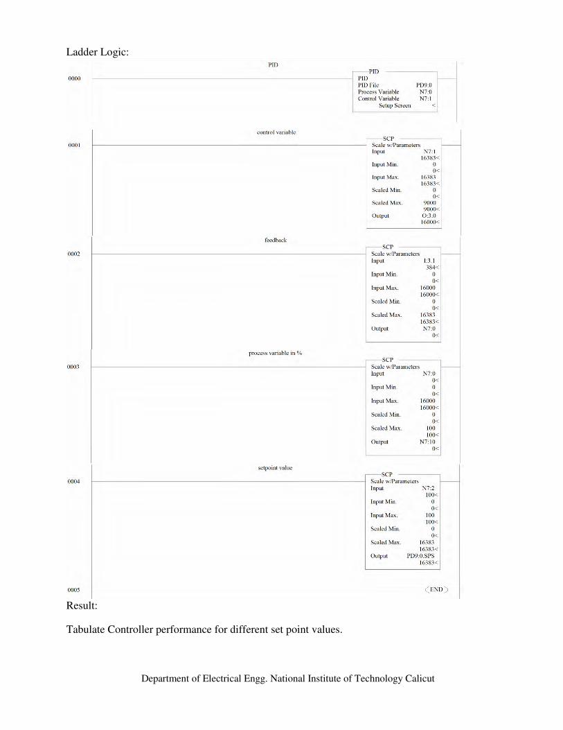
Department of Electrical Engg. National Institute of Technology Calicut
Ladder Logic:
Result:
Tabulate Controller performance for different set point values.

Department of Electrical Engg. National Institute of Technology Calicut
Exp No: BATCH PROCESS REACTOR USING Date:
PROGRAMMABLE LOGIC CONTROLLER
Aim:
To control the batch process reactor (VPAT 05) using programmable logic controller.
Apparatus required:
1. Batch process trainer kit
2. PLC (Allen Bradley Micrologix 1500 LRP series C)
3. PC with Versapro Software
4. RS232 cable
5. Patch chords
Procedure:
1. Load the Versapro software to the PC
2. Open the Versapro software
3. Switch On the PLC trainer and lift controls system
4. Connect PLC with Batch process control kit.
5. Open the New folder and draw the ladder logic program
6. Select the correct hardware configuration.
7. Store the Program to PLC
8. Run the program
9. Verify the performance to the Batch process control.
Process description:
Batch process reactor is a blending process, where two liquids are mixed together to get
the output mixture. The programmable logic controller is used to control the whole process. The
process tanks 1 & 2 consist of two liquids, which are blended in process tank 3. The process tank
1 & 2 consists of a low liquid level sensor and a high liquid level sensor. The liquids are pumped
to the process tanks using respective pumps.
The two liquids are mixed in the process tank 3 using a stirrer. Heater is used to heat the mixture.
The solenoid valves provide the liquids to the process tank 3 when the mixture level is low.
Solenoid valve 3 is connected to the output of the process tank 3, which feeds mixed liquid to a
vessel when it is sensed by the vessel proximity sensor. The container is fed through a conveyor
belt run by stepper motor. Two solenoid valves 1 & 2 control the flow of two liquids to the tank
3. The level sensors sense the level in the process tanks 1,2&3. The level sensor is a magnetic
sensor and when the liquid level is above the high level sensor a HL (high level) signal is send to
the PLC. When the liquid level goes down the low level sensor LL (low level) signal is send to
the PLC. The PLC checks the signals send by these sensors through its input port and give the
proper signals through its output port as per the ladder logic program.

Department of Electrical Engg. National Institute of Technology Calicut
Various process control actions done by the PLC are
1. When the low level sensor is sensed respective pump is on.
2. When the high level sensor is sensed respective pump is off
3. When the low level sensor in process plant 3 is sensed solenoid valve 1 and solenoid
valve 2 are made ON. (The duration of each valve in ON condition depends on its
composition)
4. When the proximity sensor senses a level, solenoid valve 3 is made on for a particular
time as set in the program.
5. Process is on a stepper motor is made ON to run the conveyor belt.

Department of Electrical Engg. National Institute of Technology Calicut
Ladder Logic:
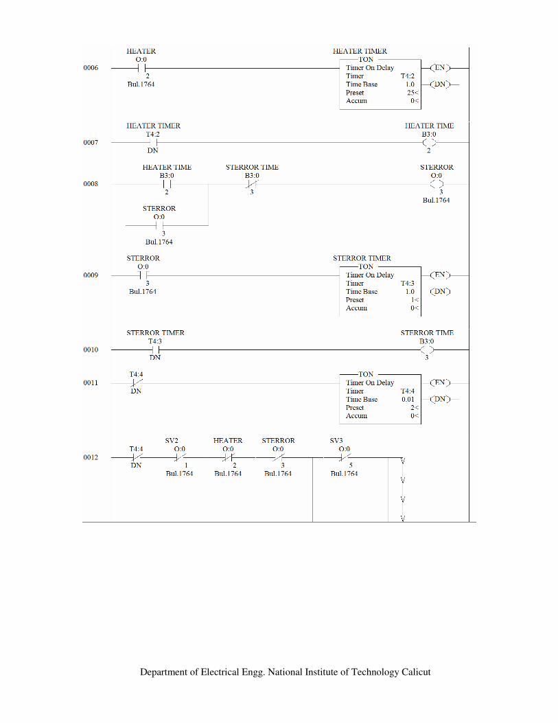
Department of Electrical Engg. National Institute of Technology Calicut
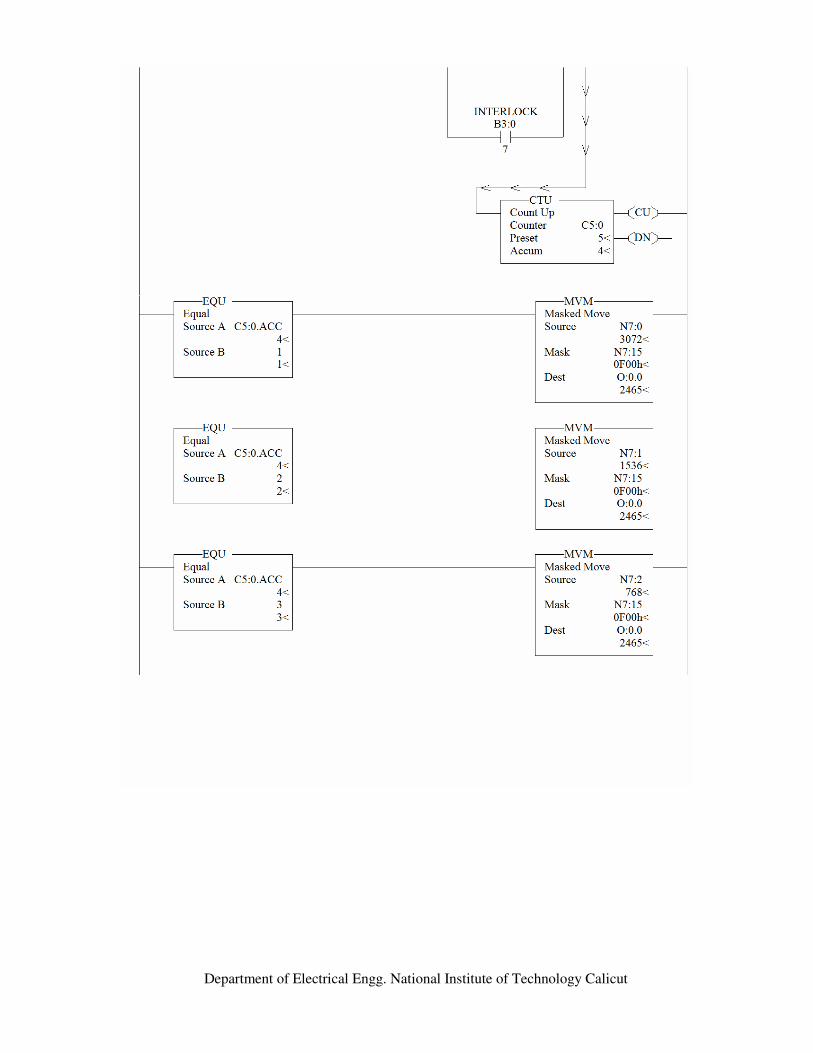
Department of Electrical Engg. National Institute of Technology Calicut

Department of Electrical Engg. National Institute of Technology Calicut

Department of Electrical Engg. National Institute of Technology Calicut
The block diagram of the batch process reactor is shown below
BATCH PROCESS REACTOR T RAINER ( VPAT 05)
Plant
1
Plant 2
Plant
resorvior
Conveyor
Stirrer
Valve
Pump 1 & 2
Valve
HEATER
Result:
The Batch process reactor was set up and controlled by using PLC ladder logic program.
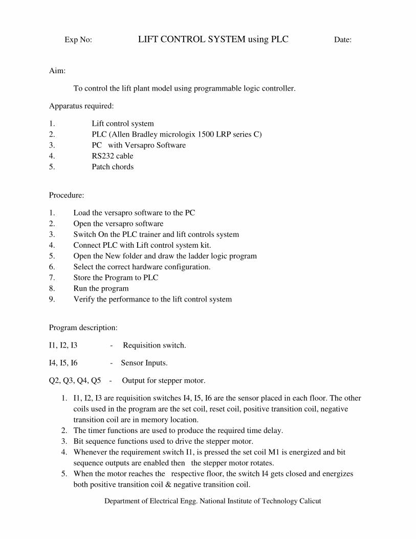
Department of Electrical Engg. National Institute of Technology Calicut
Exp No: LIFT CONTROL SYSTEM using PLC Date:
Aim:
To control the lift plant model using programmable logic controller.
Apparatus required:
1. Lift control system
2. PLC (Allen Bradley micrologix 1500 LRP series C)
3. PC with Versapro Software
4. RS232 cable
5. Patch chords
Procedure:
1. Load the versapro software to the PC
2. Open the versapro software
3. Switch On the PLC trainer and lift controls system
4. Connect PLC with Lift control system kit.
5. Open the New folder and draw the ladder logic program
6. Select the correct hardware configuration.
7. Store the Program to PLC
8. Run the program
9. Verify the performance to the lift control system
Program description:
I1, I2, I3 - Requisition switch.
I4, I5, I6 - Sensor Inputs.
Q2, Q3, Q4, Q5 - Output for stepper motor.
1. I1, I2, I3 are requisition switches I4, I5, I6 are the sensor placed in each floor. The other
coils used in the program are the set coil, reset coil, positive transition coil, negative
transition coil are in memory location.
2. The timer functions are used to produce the required time delay.
3. Bit sequence functions used to drive the stepper motor.
4. Whenever the requirement switch I1, is pressed the set coil M1 is energized and bit
sequence outputs are enabled then the stepper motor rotates.
5. When the motor reaches the respective floor, the switch I4 gets closed and energizes
both positive transition coil & negative transition coil.

Department of Electrical Engg. National Institute of Technology Calicut
6. The positive transition coil energizes one more set coil, which is used to enable the timer.
7. This is used to give time delay for the lift in each floor.
8. The negative transition coil, which was energized, is used to reset the requisition.
9. The above functions are repeated in each floor.
Conditions for rotation of Motor:
1. Consider the lift is in ground floor, when the requisition is given from first floor or
second floor the motor has to move forward.
2. If the lift is in top floor then it has to move in the reverse direction.
3. If the lift is in middle floor then according to the requisition, lift will move in forward or
reverse direction.
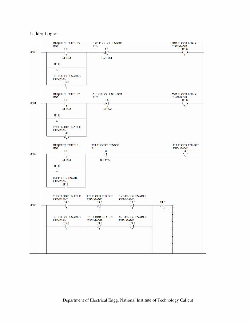
Department of Electrical Engg. National Institute of Technology Calicut
Ladder Logic:

Department of Electrical Engg. National Institute of Technology Calicut

Department of Electrical Engg. National Institute of Technology Calicut

Department of Electrical Engg. National Institute of Technology Calicut
Result:
It is observed that lift is controlled smoothly by using programmable logic controller.

Department of Electrical Engg. National Institute of Technology Calicut
Variable Frequency Drive Experiments
Introduction
A variable-frequency drive (VFD) is a system for controlling the rotational speed of an
alternating current (AC) electric motor by controlling the frequency of the electrical power
supplied to the motor. A variable frequency drive is a specific type of adjustable-speed drive.
Variable frequency drives are also known as adjustable frequency drives (AFD), variable-speed
drives (VSD), AC drives, micro drives or inverter drives. Since the voltage is varied along with
frequency, these are sometimes also called VVVF (variable voltage variable frequency) drives.
Variable-frequency drives are widely used. For example, in ventilations systems for large
buildings, variable-frequency motors on fans save energy by allowing the volume of air moved
to match the system demand. Variable frequency drives are also used on pumps, conveyor and
machine tool drives.
Operating principle
The synchronous speed of an AC motor is determined by the frequency of the AC supply and the
number of poles in the stator winding, according to the relation:
Where RPM = Revolutions per minute, f = AC power frequency (hertz), p = Number of poles (an
even number).
The constant, 120, is 60 cycles per minute multiplied by 2 poles per pole pair. Sometimes 60 is
used as the constant and p is stated as pole pairs rather than poles. By varying the frequency of
the voltage applied to the motor, its speed can be changed. Synchronous motors operate at the
synchronous speed determined by the above equation. The speed of an induction motor is
slightly less than the synchronous speed.
An inverter is an electronic power unit for generating AC power. By using an
inverter-type AC drive, the speed of a conventional AC motor can be varied through a wide
speed range from zero through the base (60 Hz) speed and above (often to 90 or 120 hertz).
When the frequency applied to an induction motor is reduced, the applied voltage must also be
reduced to limit the current drawn by the motor at reduced frequencies. (The inductive reactance
of an AC magnetic circuit is directly proportional to the frequency according to the formula, XL
= 2 ∏ f L . Variable speed AC drives will maintain a constant volts/hertz relationship from 0 - 60
Hertz. To calculate this ratio divides the motor voltage by 60 Hz. At low frequencies the voltage
will be low, as the frequency increases the voltage will increase. (Note: this ratio may be varied
somewhat to alter the motor performance characteristics such a providing a low-end boost to

Department of Electrical Engg. National Institute of Technology Calicut
improve starting torque.) Depending on the type of AC Drive, the microprocessor control adjusts
the output voltage waveform, by one of several methods, to simultaneously change the voltage
and frequency to maintain the constant volts/hertz ratio throughout the 0 - 60 Hz range. On most
AC variable speed drives the voltage is held constant above the 60 hertz frequency. The diagram
below illustrates this voltage/frequency relationship.
In Constant Torque Area - VFD supplies rated motor nameplate voltage and motor
develops full horsepower at 60 hertz base frequency. In Constant Horsepower Area - VFD
delivers motor nameplate rated voltage from 60 Hertz to 120 hertz (or drive maximum). Motor
horsepower is constant in this range but motor torque is reduced as frequency increases.
Initially standard AC motors were employed on inverter drives. Most motor
manufacturers now offer Inverter Duty Motors which provide improved performance and
reliability when used in Variable Frequency Applications. These special motors have insulation
designed to withstand the steep-wave-front voltage impressed by the VFD waveform, and are
redesigned to run smoother and cooler on inverter power supplies.
Variable VFD types
All VFDs use their output devices (IGBTs, transistors, thyristors) only as switches,
turning them only on or off. Attempting to use a linear device such as transistor in its linear
mode would be impractical, since power dissipated in the output devices would be about as much
as power delivered to the load.
Drives can be classified as: Constant voltage, Constant current, Cycloconverter
In a constant voltage converter, the intermediate DC link voltage remains approximately constant
during each output cycle.
In constant current drives, a large inductor is placed between the input rectifier and the output
bridge, so the current delivered is nearly constant.
A cycloconverter has no input rectifier or DC link and instead connects each output terminal to
the appropriate input phase.
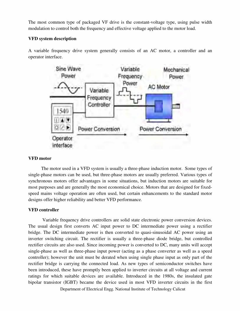
Department of Electrical Engg. National Institute of Technology Calicut
The most common type of packaged VF drive is the constant-voltage type, using pulse width
modulation to control both the frequency and effective voltage applied to the motor load.
VFD system description
A variable frequency drive system generally consists of an AC motor, a controller and an
operator interface.
VFD motor
The motor used in a VFD system is usually a three-phase induction motor. Some types of
single-phase motors can be used, but three-phase motors are usually preferred. Various types of
synchronous motors offer advantages in some situations, but induction motors are suitable for
most purposes and are generally the most economical choice. Motors that are designed for fixed-
speed mains voltage operation are often used, but certain enhancements to the standard motor
designs offer higher reliability and better VFD performance.
VFD controller
Variable frequency drive controllers are solid state electronic power conversion devices.
The usual design first converts AC input power to DC intermediate power using a rectifier
bridge. The DC intermediate power is then converted to quasi-sinusoidal AC power using an
inverter switching circuit. The rectifier is usually a three-phase diode bridge, but controlled
rectifier circuits are also used. Since incoming power is converted to DC, many units will accept
single-phase as well as three-phase input power (acting as a phase converter as well as a speed
controller); however the unit must be derated when using single phase input as only part of the
rectifier bridge is carrying the connected load. As new types of semiconductor switches have
been introduced, these have promptly been applied to inverter circuits at all voltage and current
ratings for which suitable devices are available. Introduced in the 1980s, the insulated gate
bipolar transistor (IGBT) became the device used in most VFD inverter circuits in the first
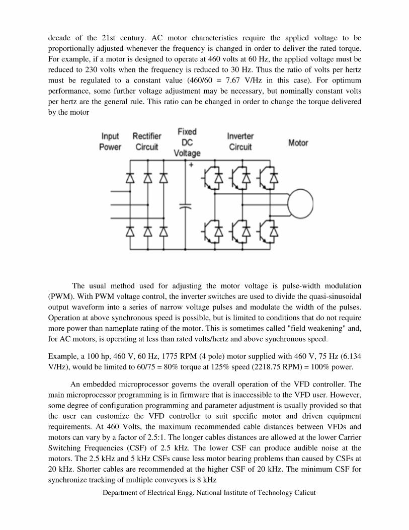
Department of Electrical Engg. National Institute of Technology Calicut
decade of the 21st century. AC motor characteristics require the applied voltage to be
proportionally adjusted whenever the frequency is changed in order to deliver the rated torque.
For example, if a motor is designed to operate at 460 volts at 60 Hz, the applied voltage must be
reduced to 230 volts when the frequency is reduced to 30 Hz. Thus the ratio of volts per hertz
must be regulated to a constant value (460/60 = 7.67 V/Hz in this case). For optimum
performance, some further voltage adjustment may be necessary, but nominally constant volts
per hertz are the general rule. This ratio can be changed in order to change the torque delivered
by the motor
The usual method used for adjusting the motor voltage is pulse-width modulation
(PWM). With PWM voltage control, the inverter switches are used to divide the quasi-sinusoidal
output waveform into a series of narrow voltage pulses and modulate the width of the pulses.
Operation at above synchronous speed is possible, but is limited to conditions that do not require
more power than nameplate rating of the motor. This is sometimes called "field weakening" and,
for AC motors, is operating at less than rated volts/hertz and above synchronous speed.
Example, a 100 hp, 460 V, 60 Hz, 1775 RPM (4 pole) motor supplied with 460 V, 75 Hz (6.134
V/Hz), would be limited to 60/75 = 80% torque at 125% speed (2218.75 RPM) = 100% power.
An embedded microprocessor governs the overall operation of the VFD controller. The
main microprocessor programming is in firmware that is inaccessible to the VFD user. However,
some degree of configuration programming and parameter adjustment is usually provided so that
the user can customize the VFD controller to suit specific motor and driven equipment
requirements. At 460 Volts, the maximum recommended cable distances between VFDs and
motors can vary by a factor of 2.5:1. The longer cables distances are allowed at the lower Carrier
Switching Frequencies (CSF) of 2.5 kHz. The lower CSF can produce audible noise at the
motors. The 2.5 kHz and 5 kHz CSFs cause less motor bearing problems than caused by CSFs at
20 kHz. Shorter cables are recommended at the higher CSF of 20 kHz. The minimum CSF for
synchronize tracking of multiple conveyors is 8 kHz

Department of Electrical Engg. National Institute of Technology Calicut
VFD operator interface
The operator interface, also commonly known as an HMI (Human Machine Interface),
provides a means for an operator to start and stop the motor and adjust the operating speed.
Additional operator control functions might include reversing and switching between manual
speed adjustment and automatic control from an external process control signal. The operator
interface often includes an alphanumeric display and/or indication lights and meters to provide
information about the operation of the drive. An operator interface keypad and display unit is
often provided on the front of the VFD controller. The keypad display can often be cable-
connected and mounted a short distance from the VFD controller. Most are also provided with
input and output (I/O) terminals for connecting pushbuttons, switches and other operator
interface devices or control signals. A serial communications port is also often available to allow
the VFD to be configured, adjusted, monitored and controlled using a computer.
VFD Operation
When a VFD starts a motor, it initially applies a low frequency and voltage to the motor.
The starting frequency is typically 2 Hz or less. Starting at such a low frequency avoids the high
inrush current that occurs when a motor is started by simply applying the utility (mains) voltage
by turning on a switch. When a VFD starts, the applied frequency and voltage are increased at a
controlled rate or ramped up to accelerate the load without drawing excessive current. This
starting method typically allows a motor to develop 150% of its rated torque while drawing only
50% of its rated current. When a motor is simply switched on at full voltage, it initially draws at
least 300% of its rated current while producing less than 50% of its rated torque. As the load
accelerates, the available torque usually drops a little and then rises to a peak while the current
remains very high until the motor approaches full speed. A VFD can be adjusted to produce a
steady 150% starting torque from standstill right up to full speed while drawing only 50%
current

Department of Electrical Engg. National Institute of Technology Calicut
With a VFD, the stopping sequence is just the opposite as the starting sequence. The frequency
and voltage applied to the motor are ramped down at a controlled rate. When the frequency
approaches zero, the motor is shut off. A small amount of braking torque is available to help
decelerate the load a little faster than it would stop if the motor were simply switched off and
allowed to coast. Additional braking torque can be obtained by adding a braking circuit to
dissipate the braking energy or return it to the power source.
Applications considerations
The output voltage of a PWM VFD consists of a train of pulses switched at the carrier
frequency. Because of the rapid rise time of these pulses, transmission line effects of the cable
between the drive and motor must be considered. Since the transmission-line impedance of the
cable and motor are different, pulses tend to reflect back from the motor terminals into the cable.
If the cable is long enough, the resulting voltages can produce up to twice the rated line voltage,
putting high stress on the cable and eventual insulation failure. Because of the standard ratings of
cables, this phenomenon is of little concern for 230 volt motors, may be a consideration for long
runs and 480 volt motors, and frequently a concern for 600 v motors.
Available VFD power ratings
Variable frequency drives are available with voltage and current ratings to match the
majority of 3-phase motors that are manufactured for operation from utility (mains) power. VFD
controllers designed to operate at 110 volts to 690 volts are often classified as low voltage units.
Low voltage units are typically designed for use with motors rated to deliver 0.2 kW or 1/4
horsepower (hp) up to at least 750 kW or 1000 hp.
Medium voltage VFD controllers are designed to operate at 2400/4160 volts (60 Hz), 3000 volts
(50 Hz) or up to 10 kV. In some applications a step up transformer is placed between a low
voltage drive and a medium voltage load. Medium voltage units are typically designed for use
with motors rated to deliver 375 kW or 500 hp and above. Medium voltage drives rated above 7
kV and 5000 or 10000 hp should probably be considered to be one-of-a-kind (one-off) designs.
A Few Considerations while selecting VFD for speed control
• Motors operated by VFD’s run hotter than motors operated across the line. Heat deteriorates
motor insulation over time. When supplying motors for variable frequency operation,
manufacturers typically use more expensive motors with a higher insulation class than motors
used in a similar non-drive application.
• The motor manufacturer should be consulted for operational limitations. Most variable
frequency drives restrict the minimum continuous speed to some percentage of the nameplate
speed. Below this minimum speed, temperature rise may damage the motor. Every 10oC rise
above the rated temperature in a motor reduces the insulation life by half.
• The motor manufacturer should be consulted before applying a VFD to an existing motor. In
addition to higher temperatures, non-VFD motors may have component natural frequencies

Department of Electrical Engg. National Institute of Technology Calicut
that will conflict with the drive output frequencies, resulting in noise, vibration, and premature
failure.
• Explosion proof motors must be rated as certified for VFD operation before they can be used
with a VFD. Qualified motors will state on the nameplate that they are certified as explosion
proof for VFD operation, as well as any operational limitations.
• Variable frequency drives should be placed near the motor. A large distance between the drive
unit and the motor may result in increased motor voltages and temperatures that stress the
conductor insulation. Special inverter duty motors are available that are made to withstand
these higher voltages. When installing long cables, special filters may be required to reduce
these effects.
• Another problem that has come to light in recent years is stray electrical currents induced into
the motor shaft by the variable frequency drive output signal. These stray currents cause
electrostatic discharges across the bearings, resulting in bearing damage. To avoid this
problem, brushes or slip rings are applied to provide a different path to ground for these
currents.
• Some centrifugal pumps have integral shaft driven circulation devices to support bearing or
mechanical seals. The pump manufacturer should be consulted regarding the minimum speed
at which these devices will operate properly. This newsletter touches just a few of the issues
that should be considered when applying a variable frequency drive. All of these potential
problems are avoidable by working closely with the manufacturer in the selection and
application of the drive and motor. Variable frequency drives provide very economical and
reliable control when selected properly and applied to the right applications.

Department of Electrical Engg. National Institute of Technology Calicut
Exp No: COMPARISON OF PERFORMANCE OF Date:
CENTRIFUGAL PUMP BY THROTTLING AND VARIABLE FREQUENCY
DRIVES
Aim:
To compare and study the performance of centrifugal pump by throttling and variable frequency
drives.
Objective:
1. To operate the pump to give different discharges using throttling with a valve
2. To operate the pump to give different discharges using a variable frequency drive.
3. To compare the performance of the pump with valve operation and variable frequency
drive.
Apparatus Required:
1. Centrifugal pump with starter
2. Variable Frequency Drive
3. Throttling valve
4. Power analyzer for input measurement
Motor Name Plate Details:
0.7kW, 415 V, 2870 rpm, 50 Hz, 3 phase, 6/22.5 m Head.
Tank Dimensions:
Length: 1.35m, Breadth: 0.68m, Height: 0.34m, Head: 2.8m.
Procedure:
Throttling:
Keep the valve at different position and run the pump at rated frequency. Observe and measure
the required parameters for efficiency calculation.
Variable Frequency Drive(VFD):
Run the pump at different frequency using VFD by keeping valve fully opened position. Observe
and measure the required parameters for efficiency calculation.
Calculate the efficiency for both the cases and compare the result by plotting the efficiency
curve.

Department of Electrical Engg. National Institute of Technology Calicut
Observation:
Throttling:
Sl
No
Valve Position
Initial
Height
(cm)
Final
Height
(cm)
Time
Required
(sec)
Discharge
m3/s
Head
(m)
O/p
(W)
I/p
(W)
η
1 Fully Opened
2 Quarter Closed
3 Half Closed
4 Quarter Opened
Variable frequency drive:
Sl
No
Frequency
(Hz)
Initial
Height
(cm)
Final
Height
(cm)
Time
Required
(sec)
Discharge
m3/s
Head
(m)
O/p
(W)
I/p
(W)
η
1
2
3
4
5
6
7
Sample Calculation:
Discharge = Volume of water pumped/ Time
= (Final Height-Initial Height) * Base Area of the tank / Time
= ……..m3/sec
Output = Water Density * Discharge * g * Head

Department of Electrical Engg. National Institute of Technology Calicut
= ……….watts
Input = …… watts
Efficiency = (Output power) / (Input power) x 100 %
output vs efficeincy
0
5
10
15
20
25
30
35
40
45
50
0 20 40 60 80 100 120
output in watts
% e
ffic
ien
cy
throttling
vfd
Result:
The performance of the centrifugal pump with throttling and variable frequency drive is studied.

Department of Electrical Engg. National Institute of Technology Calicut
Microcontroller Experiments
80196 Microcontrollers
Architecture
The 80c196 is mainly based on :
A CPU which is turn composed of a 16-bit ALU with temporary registers, a 256-byte RAM
used as 24 special registers and 232 general registers, and a microprogrammed sequencer.
A memory controller with a 4-byte FIFO queue to prefetch instructions and data from the
programmemory.
A set of I/O interfaces.
The CPU gets his information only through the memory controller and the special registers also
called Special Function Registers (SFRs).
The ALU, is associated to a set of temporary registers (with shifter, counter, constants) and thus
called RALU (Register ALU). The RALU doesn't use an accumulator but instead is ablt to
directly work with any of the 256 special or general registers
All I/O operations are controlled through the SFRs.

Department of Electrical Engg. National Institute of Technology Calicut
Memory controller
All of the program memory and external data memory are transferred to the CPU through the
memory controller. The memory controller consists of a slave program counter, an instruction
queue and a bus controller. The slave program counter keeps track of the instructions fetched
from the program memory. Instructions fetched by the memory controller are stored in the
queue. The slave program counter may be up to four bytes ahead of the main program counter
(which is located in the RALU), because it is pre-fetching the instructions. The bus controller
access program memory (on-chip EPROM) and external data memory and arbitrates between
instruction fetches and data reads and writes. The bus controller supports both 8-bit and 16-bit
external bus modes. Memory access requests to the bus controller can come from either the
RALU or the queue, with priority given to the queue accesses. If the address sequence changes
because of a jump interrupt, call or return, the slave PC is loaded with a new value, and the
queue is flushed. Reloading the slave PC, flushing the queue and fetching the first byte of the
new instruction stream takes 4 state times. This is reflected in the conditional jump taken/not-
taken execution times.
The CPU
The CPU is controlled by a microcode sequencer and can perform operations on any byte, word
or double-word in the 256-byte register space. Instructions to the CPU are taken from the pre-
fetch queue and temporarily stored in the instruction register. The sequencer decodes the
instruction and generates the correct sequence of events to have the RALU perform the desired
operation.
The RALU
Most calculations performed by the 80c196 take place in the RALU. The RALU contains a 17-
bit ALU - Arithmetic and Logic Unit, the flag register also called PSW - Program Status Word,
the main PC - Program Counter, a loop counter and three temporary registers. All registers are
16-bits or 17-bits wide. The PC has a separate incrementor as to access operands. However, PC
changes due to jumps, interrupts, calls and returns are handled through the ALU. Two of the
temporary registers have their own shift logic. These registers are used for the instructions which
require logical shifts, including Normalize, Multiply and Divide. The upper word and lower
word registers are used together for the 32-bit instructions and as temporary registers for many
other instructions. Repetitive shifts are counted by the 6-bit loop counter. A third temporary
register stores the second operand of two-operand instructions. To perform subtractions the
output of this register can be complemented before being placed into the input of the ALU. The
RALU also stores several constants such as 0,1 and 2 to speed up certain operations like getting a
2's complement, incrementing or decrementing.

Department of Electrical Engg. National Institute of Technology Calicut
The
Register Arithmetic and Logic Unit
Addressable space
The addressable memory space of the 80c196 consists of 64k bytes. However, not all these
addresses are available to the user. Addresses 0000H through 00FFH and 1FFEH through 207FH
are reserved for special purposes. All other locations can be used for either program or data
storage, or for memory-mapped I/O.
FFFFH +-------------------------+
| |
| External memory or I/O |
| |
4000H +-------------------------+
| Internal ROM/EPROM or |
| external memory or I/O |
2080H +-------------------------+
| Reserved |
2040H +-------------------------+
| 8 interrupt vectors |
2030H +-------------------------+
| ROM/EPROM security key |
2020H +-------------------------+
| Reserved |
2019H +-------------------------+
| Chip Configuration byte |
2018H +-------------------------+
| Reserved |
2014H +-------------------------+
| 10 interrupt vectors |
2000H +-------------------------+
| Port 3 and port 4 |
1FFEH +-------------------------+
| External memory or I/O |
0200H +-------------------------+

Department of Electrical Engg. National Institute of Technology Calicut
| 80c196KC internal RAM |
0100H +-------------------------+
| Registers and SFRs |
0000H +-------------------------+
80c196 addressable space
Registers (internal RAM)
Locations 00H through OFFH contain the 232 general registers and the 24 SFRs - Special
Function Registers. The RALU can operate on any of these 256 internal register locations, but
code cannot be executed from them. If attempt is made to execute instructions from locations 00H
through OFFH, the instructions will be fetched from external memory. This section of external
memory is generally used by the Intel development tools. Locations 018H through OFFH are the
general registers. These locations can be accessed as byte, word or double-word registers, and
can be essentially considered as 232 accumulators. Locations 018H and O19H contain the stack
pointer. Operations to the stack cause it to be built down and the stack pointer is pre-
decremented, so the stack must be initialized by the user program to 2 bytes above the highest
stack location. The stack pointer must point to a word (even) address.
Special Function Registers (SFRs)
Locations 00H through O17H are the I/O control registers or SFRs. All of the peripheral devices
of the 80c196 except ports 3 and 4 are controlled through these registers. SFR functions are
controlled through 3 windows. Switching between the windows is done using the WSR -
Window Select Register located at address 014H. SFR windows other than WSR = 0 are out of
the scope of this course. Some of the Special Function Registers have different meanings if read
from or written to.
Reserved memory locations
Locations 1FFEH and O1FFFH are used for Ports 3 and 4 respectively. Many reserved and
special locations are in the memory area between 2000H and 2080H. The 18 interrupt vectors,
the chip configuration byte and the security key are located in this area. All the addresses marked
Reserved in this area have to be programmed with value 0FFH. 2080H is the normal program
start address. A reset interrupt restarts the program at address 2080H.
External memory
There are several modes of system bus operation on the 80c196. The standard bus mode uses a
16-bit multiplexed address/data bus. Other bus modes include an 8-bit mode and a mode in
which the bus size can be dynamically switched between 8-bits and 16-bits. In addition, there are
several options available on the type of bus control signals which make an external bus simple to
design.
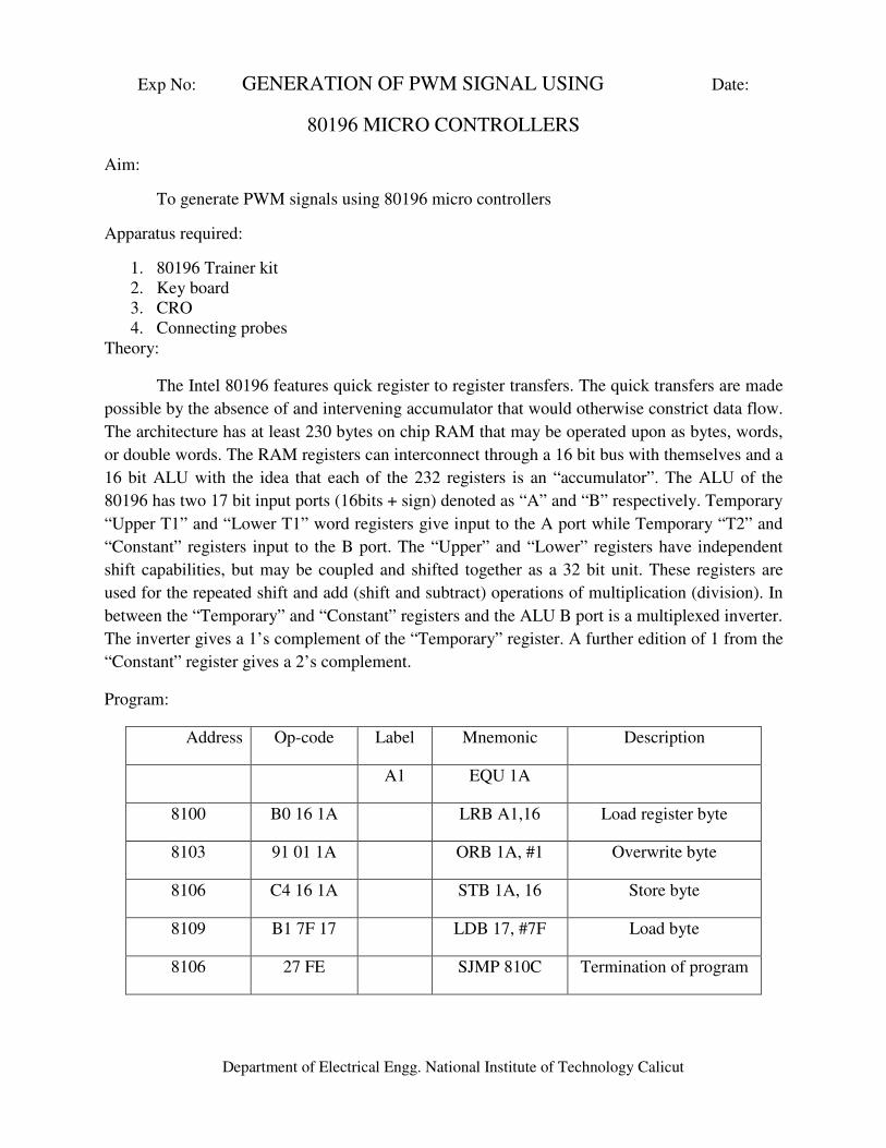
Department of Electrical Engg. National Institute of Technology Calicut
Exp No: GENERATION OF PWM SIGNAL USING Date:
80196 MICRO CONTROLLERS
Aim:
To generate PWM signals using 80196 micro controllers
Apparatus required:
1. 80196 Trainer kit
2. Key board
3. CRO
4. Connecting probes
Theory:
The Intel 80196 features quick register to register transfers. The quick transfers are made
possible by the absence of and intervening accumulator that would otherwise constrict data flow.
The architecture has at least 230 bytes on chip RAM that may be operated upon as bytes, words,
or double words. The RAM registers can interconnect through a 16 bit bus with themselves and a
16 bit ALU with the idea that each of the 232 registers is an “accumulator”. The ALU of the
80196 has two 17 bit input ports (16bits + sign) denoted as “A” and “B” respectively. Temporary
“Upper T1” and “Lower T1” word registers give input to the A port while Temporary “T2” and
“Constant” registers input to the B port. The “Upper” and “Lower” registers have independent
shift capabilities, but may be coupled and shifted together as a 32 bit unit. These registers are
used for the repeated shift and add (shift and subtract) operations of multiplication (division). In
between the “Temporary” and “Constant” registers and the ALU B port is a multiplexed inverter.
The inverter gives a 1’s complement of the “Temporary” register. A further edition of 1 from the
“Constant” register gives a 2’s complement.
Program:
Address Op-code Label Mnemonic Description
A1 EQU 1A
8100 B0 16 1A LRB A1,16 Load register byte
8103 91 01 1A ORB 1A, #1 Overwrite byte
8106 C4 16 1A STB 1A, 16 Store byte
8109 B1 7F 17 LDB 17, #7F Load byte
8106 27 FE SJMP 810C Termination of program

Department of Electrical Engg. National Institute of Technology Calicut
Procedure:
1. Enter the above program
2. Using an oscilloscope, observe the PWM output at 12th
pin of the analog I/O
connector P2 (now the duty cycle is 50%)
Output:
Frequency:
Amplitude:
Result:
PWM signal is generated using 80196 micro controller kit, with 50% duty ratio.
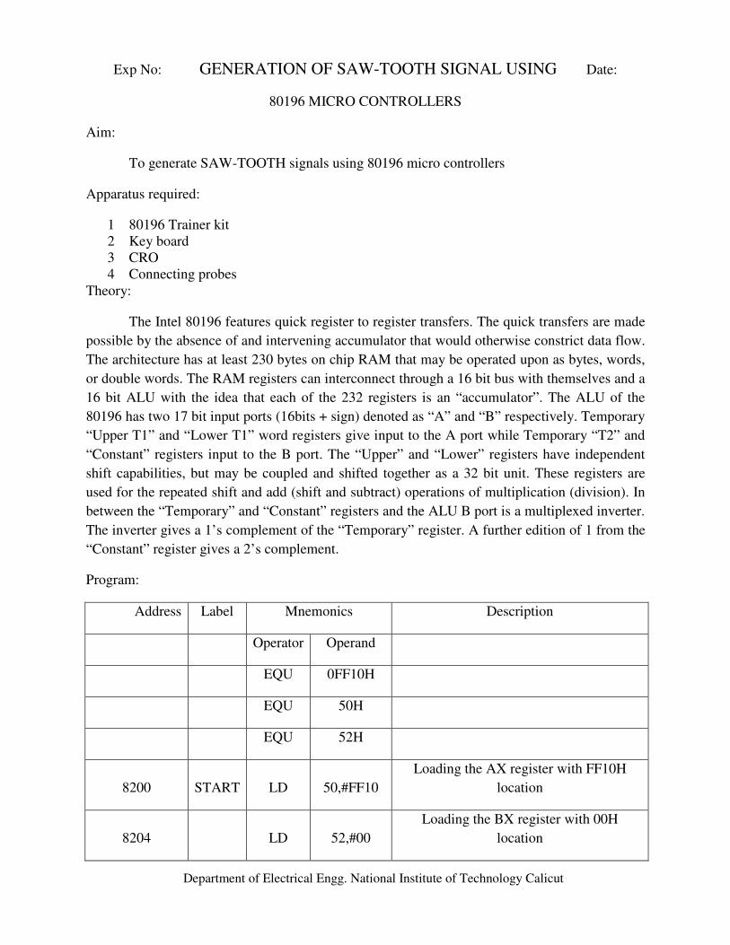
Department of Electrical Engg. National Institute of Technology Calicut
Exp No: GENERATION OF SAW-TOOTH SIGNAL USING Date:
80196 MICRO CONTROLLERS
Aim:
To generate SAW-TOOTH signals using 80196 micro controllers
Apparatus required:
1 80196 Trainer kit
2 Key board
3 CRO
4 Connecting probes
Theory:
The Intel 80196 features quick register to register transfers. The quick transfers are made
possible by the absence of and intervening accumulator that would otherwise constrict data flow.
The architecture has at least 230 bytes on chip RAM that may be operated upon as bytes, words,
or double words. The RAM registers can interconnect through a 16 bit bus with themselves and a
16 bit ALU with the idea that each of the 232 registers is an “accumulator”. The ALU of the
80196 has two 17 bit input ports (16bits + sign) denoted as “A” and “B” respectively. Temporary
“Upper T1” and “Lower T1” word registers give input to the A port while Temporary “T2” and
“Constant” registers input to the B port. The “Upper” and “Lower” registers have independent
shift capabilities, but may be coupled and shifted together as a 32 bit unit. These registers are
used for the repeated shift and add (shift and subtract) operations of multiplication (division). In
between the “Temporary” and “Constant” registers and the ALU B port is a multiplexed inverter.
The inverter gives a 1’s complement of the “Temporary” register. A further edition of 1 from the
“Constant” register gives a 2’s complement.
Program:
Address Label Mnemonics Description
Operator Operand
EQU 0FF10H
EQU 50H
EQU 52H
8200 START LD 50,#FF10
Loading the AX register with FF10H
location
8204 LD 52,#00
Loading the BX register with 00H
location

Department of Electrical Engg. National Institute of Technology Calicut
8208 ST 52,[50]
Storing Accumulator content to BX
register
820B ADD 52,#01 Pointing BX register to next location
820F CMP 52,#0FFFH Comparing BX location with 0FFFH
8213 JNE 8208 Jump to location 8208H
8215 SJMP START To get next cycle
Procedure:
1 Enter the above program
2 Using an oscilloscope, observe the SAW-TOOTH output at the port
Output:
Frequency:
Amplitude:
Result:
The SAW-TOOTH wave is generated using 80196 micro controller kit

Department of Electrical Engg. National Institute of Technology Calicut
80C51 Microcontroller
Memory Organization
All 80C51 devices have separate address spaces for program and data memory, as shown in
Figures 1 and 2. The logical separation of program and data memory allows the data memory to
be accessed by 8-bit addresses, which can be quickly stored and manipulated by an 8-bit CPU.
Nevertheless, 16-bit data memory addresses can also be generated through the DPTR register.
Program memory (ROM, EPROM) can only be read, not written to. There can be up to 64k bytes
of program memory. In the 80C51, the lowest 4k bytes of program are on-chip. In the ROM less
versions, all program memory is external. The read strobe for external program memory is the
PSEN (program store enable). Data Memory (RAM) occupies a separate address space from
Program Memory. In the 80C51, the lowest 128 bytes of data memory are on-chip. Up to 64k
bytes of external RAM can be addressed in the external Data Memory space. In the ROM less
version, the lowest 128 bytes are on-chip. The CPU generates read and write signals, RD and
WR, as needed during external Data Memory accesses. External Program Memory and external
Data Memory may be combined if desired by applying the RD and PSEN signals to the inputs of
an AND gate and using the output of the gate as the read strobe to the external Program/Data
memory.

Department of Electrical Engg. National Institute of Technology Calicut
Program Memory
Figure 3 shows a map of the lower part of the Program Memory. After reset, the CPU begins
execution from location 0000H. As shown in Figure 3, each interrupt is assigned a fixed location
in Program Memory. The interrupt causes the CPU to jump to that location, where it commences
execution of the service routine. External Interrupt 0, for example, is assigned to location 0003H.
If External Interrupt 0 is going to be used, its service routine must begin at location 0003H. If the
interrupt is not going to be used, its service location is available as general purpose Program
Memory.
The interrupt service locations are spaced at 8-byte intervals: 0003H for External Interrupt 0,
000BH for Timer 0, 0013H for External Interrupt 1, 001BH for Timer 1, etc. If an interrupt
service routine is short enough (as is often the case in control applications), it can reside entirely
within that 8-byte interval. Longer service routines can use a jump instruction to skip over
subsequent interrupt locations, if other interrupts are in use.
The lowest 4k bytes of Program Memory can either be in the on-chip ROM or in an external
ROM. This selection is made by strapping the EA (External Access) pin to either VCC, or VSS.
In the 80C51, if the EA pin is strapped to VCC, then the program fetches to addresses 0000H
through 0FFFH are directed to the internal ROM. Program fetches to addresses 1000H through
FFFFH are directed to external ROM.
If the EA pin is strapped to VSS, then all program fetches are directed to external ROM. The
ROM less parts (8031, 80C31, etc.) must have this pin externally strapped to VSS to enable them
to execute from external Program Memory.

Department of Electrical Engg. National Institute of Technology Calicut
The read strobe to external ROM, PSEN, is used for all external program fetches. PSEN is not
activated for internal program fetches. The hardware configuration for external program
execution is shown in Figure 4. Note that 16 I/O lines (Ports 0 and 2) are dedicated to bus
functions during external Program Memory fetches. Port 0 (P0 in Figure 4) serves as a
multiplexed address/data bus. It emits the low byte of the Program Counter (PCL) as an address,
and then goes into a float state awaiting the arrival of the code byte from the Program Memory.
During the time that the low byte of the Program Counter is valid on Port 0, the signal ALE
(Address Latch Enable) clocks this byte into an address latch. Meanwhile, Port 2 (P2 in Figure 4)
emits the high byte of the Program Counter (PCH). Then PSEN strobes the EPROM and the
code byte is read into the microcontroller.
Program Memory addresses are always 16 bits wide, even though the actual amount of Program
Memory used may be less than 64k bytes. External program execution sacrifices two of the 8-bit
ports, P0 and P2, to the function of addressing the Program Memory.
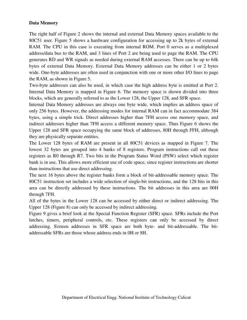
Department of Electrical Engg. National Institute of Technology Calicut
Data Memory
The right half of Figure 2 shows the internal and external Data Memory spaces available to the
80C51 user. Figure 5 shows a hardware configuration for accessing up to 2k bytes of external
RAM. The CPU in this case is executing from internal ROM. Port 0 serves as a multiplexed
address/data bus to the RAM, and 3 lines of Port 2 are being used to page the RAM. The CPU
generates RD and WR signals as needed during external RAM accesses. There can be up to 64k
bytes of external Data Memory. External Data Memory addresses can be either 1 or 2 bytes
wide. One-byte addresses are often used in conjunction with one or more other I/O lines to page
the RAM, as shown in Figure 5.
Two-byte addresses can also be used, in which case the high address byte is emitted at Port 2.
Internal Data Memory is mapped in Figure 6. The memory space is shown divided into three
blocks, which are generally referred to as the Lower 128, the Upper 128, and SFR space.
Internal Data Memory addresses are always one byte wide, which implies an address space of
only 256 bytes. However, the addressing modes for internal RAM can in fact accommodate 384
bytes, using a simple trick. Direct addresses higher than 7FH access one memory space, and
indirect addresses higher than 7FH access a different memory space. Thus Figure 6 shows the
Upper 128 and SFR space occupying the same block of addresses, 80H through FFH, although
they are physically separate entities.
The Lower 128 bytes of RAM are present in all 80C51 devices as mapped in Figure 7. The
lowest 32 bytes are grouped into 4 banks of 8 registers. Program instructions call out these
registers as R0 through R7. Two bits in the Program Status Word (PSW) select which register
bank is in use. This allows more efficient use of code space, since register instructions are shorter
than instructions that use direct addressing.
The next 16 bytes above the register banks form a block of bit-addressable memory space. The
80C51 instruction set includes a wide selection of single-bit instructions, and the 128 bits in this
area can be directly addressed by these instructions. The bit addresses in this area are 00H
through 7FH.
All of the bytes in the Lower 128 can be accessed by either direct or indirect addressing. The
Upper 128 (Figure 8) can only be accessed by indirect addressing.
Figure 9 gives a brief look at the Special Function Register (SFR) space. SFRs include the Port
latches, timers, peripheral controls, etc. These registers can only be accessed by direct
addressing. Sixteen addresses in SFR space are both byte- and bit-addressable. The bit-
addressable SFRs are those whose address ends in 0H or 8H.

Department of Electrical Engg. National Institute of Technology Calicut

Department of Electrical Engg. National Institute of Technology Calicut
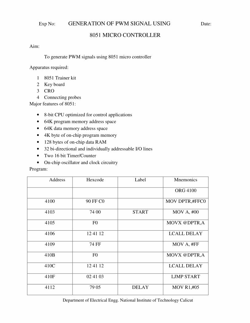
Department of Electrical Engg. National Institute of Technology Calicut
Exp No: GENERATION OF PWM SIGNAL USING Date:
8051 MICRO CONTROLLER
Aim:
To generate PWM signals using 8051 micro controller
Apparatus required:
1 8051 Trainer kit
2 Key board
3 CRO
4 Connecting probes
Major features of 8051:
• 8-bit CPU optimized for control applications
• 64K program memory address space
• 64K data memory address space
• 4K byte of on-chip program memory
• 128 bytes of on-chip data RAM
• 32 bi-directional and individually addressable I/O lines
• Two 16 bit Timer/Counter
• On-chip oscillator and clock circuitry
Program:
Address Hexcode Label Mnemonics
ORG 4100
4100 90 FF C0 MOV DPTR,#FFC0
4103 74 00 START MOV A, #00
4105 F0 MOVX @DPTR,A
4106 12 41 12 LCALL DELAY
4109 74 FF MOV A, #FF
410B F0 MOVX @DPTR,A
410C 12 41 12 LCALL DELAY
410F 02 41 03 LJMP START
4112 79 05 DELAY MOV R1,#05

Department of Electrical Engg. National Institute of Technology Calicut
4114 7A FF LOOP MOV R2, #FF
4116 DA FE DJNZ R2, HERE
4118 D9 FA DJNZ R1, LOOP
411A 22 RET
411B 80 E6 SJMP START
Procedure:
1. Enter the above program
2. Using an oscilloscope, observe the PWM output at the port
Result:
PWM signal is generated using 8051 micro controller kit with 50% duty ratio.
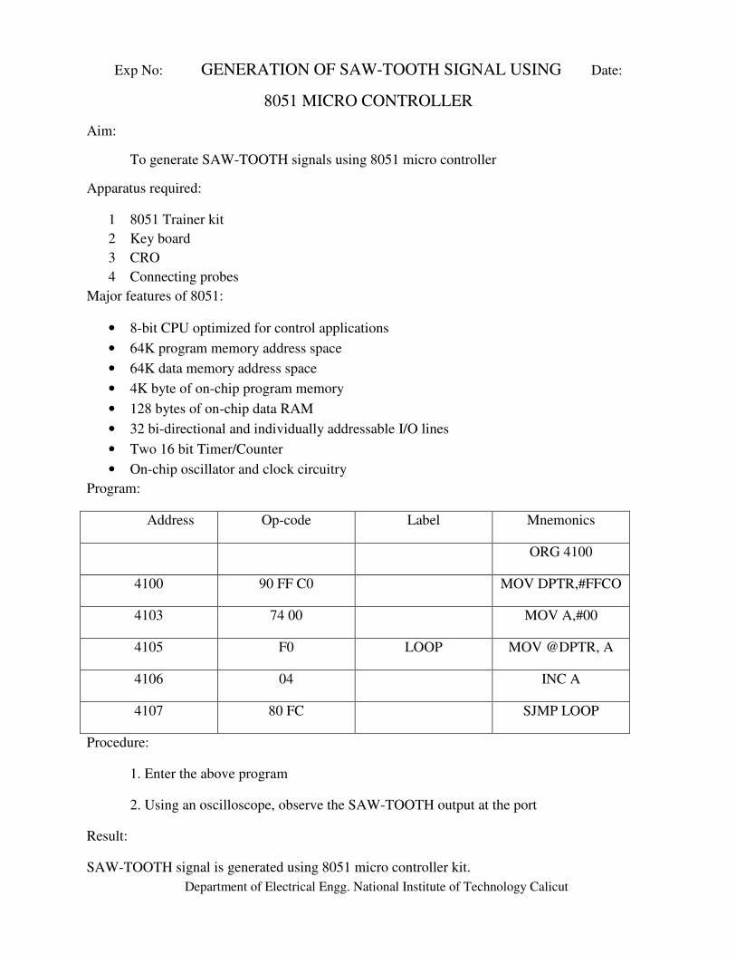
Department of Electrical Engg. National Institute of Technology Calicut
Exp No: GENERATION OF SAW-TOOTH SIGNAL USING Date:
8051 MICRO CONTROLLER
Aim:
To generate SAW-TOOTH signals using 8051 micro controller
Apparatus required:
1 8051 Trainer kit
2 Key board
3 CRO
4 Connecting probes
Major features of 8051:
• 8-bit CPU optimized for control applications
• 64K program memory address space
• 64K data memory address space
• 4K byte of on-chip program memory
• 128 bytes of on-chip data RAM
• 32 bi-directional and individually addressable I/O lines
• Two 16 bit Timer/Counter
• On-chip oscillator and clock circuitry
Program:
Address Op-code Label Mnemonics
ORG 4100
4100 90 FF C0 MOV DPTR,#FFCO
4103 74 00 MOV A,#00
4105 F0 LOOP MOV @DPTR, A
4106 04 INC A
4107 80 FC SJMP LOOP
Procedure:
1. Enter the above program
2. Using an oscilloscope, observe the SAW-TOOTH output at the port
Result:
SAW-TOOTH signal is generated using 8051 micro controller kit.
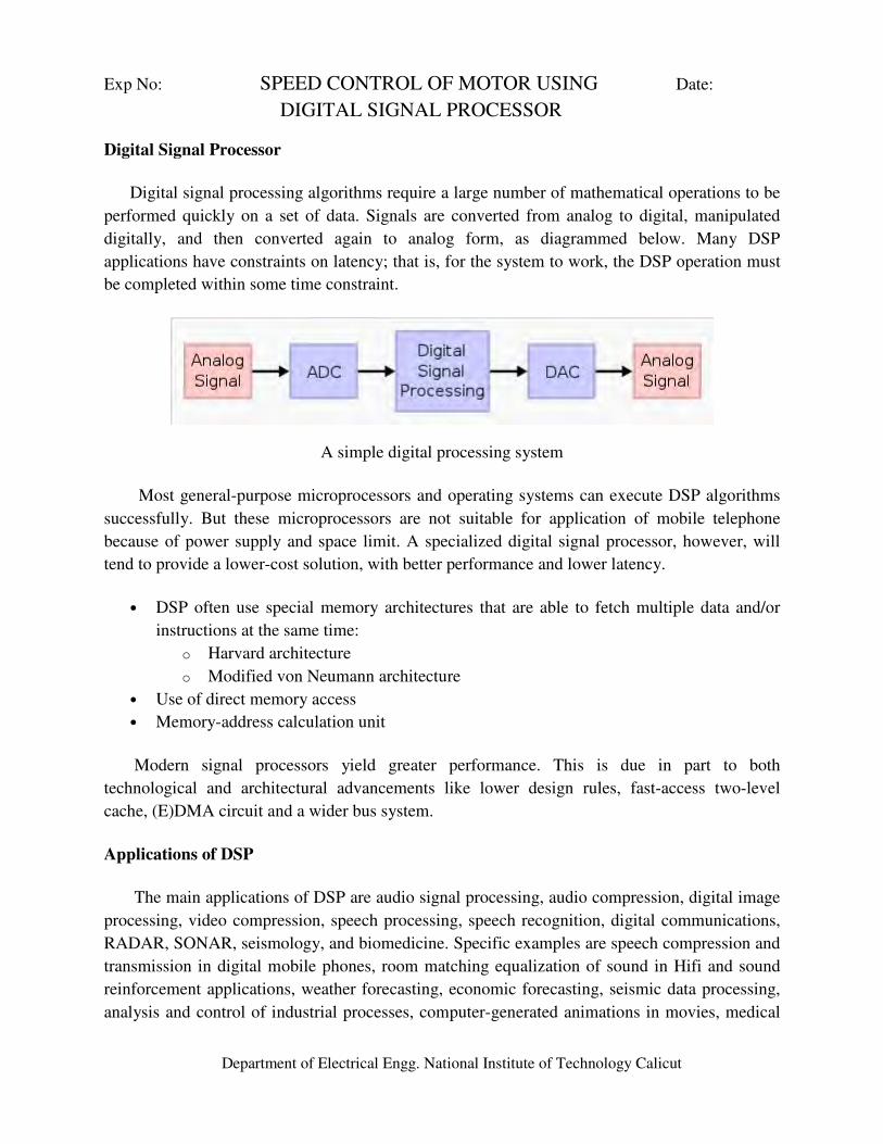
Department of Electrical Engg. National Institute of Technology Calicut
Exp No: SPEED CONTROL OF MOTOR USING Date:
DIGITAL SIGNAL PROCESSOR
Digital Signal Processor
Digital signal processing algorithms require a large number of mathematical operations to be
performed quickly on a set of data. Signals are converted from analog to digital, manipulated
digitally, and then converted again to analog form, as diagrammed below. Many DSP
applications have constraints on latency; that is, for the system to work, the DSP operation must
be completed within some time constraint.
A simple digital processing system
Most general-purpose microprocessors and operating systems can execute DSP algorithms
successfully. But these microprocessors are not suitable for application of mobile telephone
because of power supply and space limit. A specialized digital signal processor, however, will
tend to provide a lower-cost solution, with better performance and lower latency.
• DSP often use special memory architectures that are able to fetch multiple data and/or
instructions at the same time:
o Harvard architecture
o Modified von Neumann architecture
• Use of direct memory access
• Memory-address calculation unit
Modern signal processors yield greater performance. This is due in part to both
technological and architectural advancements like lower design rules, fast-access two-level
cache, (E)DMA circuit and a wider bus system.
Applications of DSP
The main applications of DSP are audio signal processing, audio compression, digital image
processing, video compression, speech processing, speech recognition, digital communications,
RADAR, SONAR, seismology, and biomedicine. Specific examples are speech compression and
transmission in digital mobile phones, room matching equalization of sound in Hifi and sound
reinforcement applications, weather forecasting, economic forecasting, seismic data processing,
analysis and control of industrial processes, computer-generated animations in movies, medical

Department of Electrical Engg. National Institute of Technology Calicut
imaging such as CAT scans and MRI, MP3 compression, image manipulation, high fidelity
loudspeaker crossovers and equalization, and audio effects for use with electric guitar amplifiers.
Implementation of DSP
Digital signal processing is often implemented using specialized microprocessors such as the
DSP56000, the TMS320, or the SHARC. These often process data using fixed-point arithmetic,
although some versions are available which use floating point arithmetic and are more powerful.
For faster applications FPGAs might be used. Beginning in 2007, multicore implementations of
DSPs have started to emerge from companies including Freescale and Stream Processors, Inc.
For faster applications with vast usage, ASICs might be designed specifically. For slow
applications, a traditional slower processor such as a microcontroller may be adequate.
Aim:
1. To control the speed of motor using DSP controller.
2. To study the variation in settling time and peak overshoot by the variation of the
PID controller settings
Apparatus required:
1. DSP Trainer Kit(TMS320F2407)
2. 3 phase induction motor (2.2kW, 415V, 4.4A, 50Hz, 1435rpm) with speed sensor
3. 3 phase autotransformer
4. IPM based power module
5. PC with DSP software(C2407 serial Monitor software)
Procedure:
1. Load the software to the PC
2. Open the software
3. Switch on the DSP trainer kit and the motor starter.
4. Connect the DSP kit and controller module
5. Open the folder and select the control required
6. Give the PID parameters
7. Run the program
8. Verify the speed response of the motor by varying the controller settings.
Description:
Speed of the AC induction motor can be controlled by varying the input voltage to the
motor. This can be achieved by using a DSP kit to produce variable voltage. Variable voltage is
produced by triggering the IGBT’s in the power module at different angles. DSP processor is
producing the necessary PWM gating signals for the IGBT triggering. Speed sensor will sense
the speed and gives equivalent voltage signals to the power module. From power module, control

Department of Electrical Engg. National Institute of Technology Calicut
signals are fed to the DSP through ADC. PWM signals from the DSP are given back to the
power module which controls the speed of the motor. Hence it is a feedback system. We can
vary the PI controller settings and verify the controller performance.
Observation:
Open loop control
P
I
D CURRENT
%
OVERSHOOT
SETTLING
TIME
Closed loop control
P
I
D
CURRENT
%
OVERSHOOT
SETTLING
TIME
Result:
Speed of AC motor is controlled by using digital signal processor. The controller settings are
varied and observed the behavior of the system according to the different settings.

Department of Electrical Engg. National Institute of Technology Calicut
Power Quality Testing Experiments
Introduction
Proliferation of non-linear loads (rectifiers, arc furnace, variable speed drives, UPS,
computers, printers, domestic electronic equipment etc.) and motors at industrial, commercial
and residential sectors over the last few years have resulted in the degradation of power quality
all over the world. These devices with power electronic controllers draw a distorted, non-
sinusoidal current waveform. The harmonics injected by these devices results in many problems
such as burning out of capacitors, increased heating loss, fire hazards, malfunctioning of
protection and control gears, metering errors, data loss in computers.
Power quality problems created by drive such as voltage surges, voltage dips, etc lead to
the malfunctioning of the sophisticated and costlier devices connected to the system. It may also
lead to cogging and crawling in motors, low starting torque etc. Motors have the undesirable
effect of drawing several times their full load current while starting, which also will lead to
voltage surges, voltage dips etc.
The poor power quality can affect the safe and reliable operation of all devices including
drives. Some of the effects of poor power quality on drives are improper start up which may
cause damage to the motor, overheating of rotors, pulsating torques, increased losses etc. Various
regulatory authorities like IES, BIS, and IEEE have brought out statutory requirements on the
amount of harmonics, sags, swells, dips etc.
Power Quality
The term ‘power quality’ has come into the vocabulary of many industrial and
commercial electricity end-users in recent years. Power quality problems can be simplistically
defined as cases where the electric quantities (voltage or current) diverge from the ideal. The
ever-expanding application of power electronic loads and the increasing dependency upon
information processing systems have produced serious concerns about power quality (PQ). The
typical power quality problems, its sources and some mitigation techniques are described below.
Types of PQ issues
The following paragraphs introduce the main definitions of power quality measurable
quantities or occurrences:
♦ A voltage dip is a reduction in the RMS voltage in the range of 0.1 to 0.9 p.u for duration
greater than half a mains cycle and less than 1 minute, often referred to as ’sag’. Caused
by faults, increased load demand and transitional events such as large motor starting.
♦ A voltage swell is an increase in the RMS voltage in the range of 1.1 to 1.8 p.u for a
duration greater than half a mains cycle and less than 1 minute. Caused by system faults,
load switching and capacitor switching.
♦ A transient is an undesirable momentary deviation of the supply voltage or load current.

Department of Electrical Engg. National Institute of Technology Calicut
♦ Harmonics are periodic sinusoidal distortions of the supply voltage or load current caused
by non-linear loads. Harmonics are measured in integer multiples of fundamental supply
frequency. The distortion factor or total harmonic distortion may be defined as
2
1
2
2
a
a
THD nn∑
∞
== where n=2,3,4….
componentlfundumemtatheofmagnitudea
sfrequencieharmonictheofmagnitudean
=
=
1
♦ Voltage unbalance is defined as a deviation in the magnitude and/or phase of one or more
of the phases, of a three-phase supply, with respect to the magnitude of the other phases
and the normal phase angle (120°).
♦ Frequency deviation is a variation of frequency from the sinusoidal supply frequency
above/below a predetermined level, normally ±0.1%.
♦ A transient interruption is defined as a reduction in the supply voltage, or load current, to
a level less than 0.1 p.u. for a time of not more than 1 minute. Interruptions can be caused
by system faults, system equipment failures or control and protection malfunctions.
♦ A flicker can be defined as the perceptible change in a lamp output produced by a sudden
change in supply voltage, caused by the loads like arc furnaces and pulsating loads.
♦ An outage is defined as an interruption that has duration lasting in excess of one minute.
♦ An under voltage is a drop in service voltage below the proper nominal operating low
voltage limit for several seconds in duration.
♦ An over voltage is the steady state voltage for several seconds or longer which is above
the upper source voltage limit. Over voltages usually occurs due to the improper
adjustment of voltage regulators, capacitors etc.
Sources of PQ issues
The sources of power quality problems are discussed as follows.
Power electronic devices:
Power electronic devices are non-linear loads that create harmonic distortion and can be
susceptible to voltage dips if not adequately protected. The most common ‘economically
damaging’ power quality problem encountered involves the use of variable-speed drives.
Variable-speed motor drives or inverters are highly susceptible to voltage dip disturbances
and cause particular problems in industrial processes where loss of mechanical synchronism
is an issue.

Department of Electrical Engg. National Institute of Technology Calicut
IT and office equipment:
IT equipment power supplies consist of a switched mode power supply (SMPS) and are the
cause of a significant increase in the level of 3rd, 5th and 7th harmonic voltage distortion in
recent years. Because the third harmonic is a ‘triplen’ harmonic it is of zero order phase
sequence and therefore adds in the neutral of a balanced three-phase system.
Arcing devices:
Electric arc furnaces, arc welders and electric discharge lamps are all forms of electric
arcing device. These devices are highly non-linear loads. All arcing devices are sources of
harmonic distortion. The arcing load can be represented as a relatively stable source of voltage
harmonics. The effects of arc furnaces are difficult to mitigate. Arc welders commonly cause
transients in the local network due to the intermittent switching and therefore some electronic
equipment may require protection from the impulsive spikes generated.
Load switching:
The effect of heavy load switching on the local network is a fairly common problem
causing transients to propagate to other ‘electrically close’ equipment. These transients can be of
surprisingly large voltage magnitude, but have very little energy due to their short duration,
which is normally measured in terms of milliseconds. Electronic devices that may be sensitive to
these voltage impulses can have their operation impaired. This type of transient might occur as
the result of switching in a heavy single-phase load, the effect seen on the voltage measured
nearby other equipment can be protected from these switching transients by electrically isolating
them from the affecting equipment.
Larger motor starting:
The dynamic nature of induction machines means that they draw current depending on the
mode of operation; during starting this current can be as high as six times the normal rated
current. This increased loading on the local network has the effect of causing a voltage dip, the
magnitude of which is dependent on the system impedance. Most modern motors employ a
sophisticated power electronic converter ‘drive’, which in most cases will control the motor’s
starting current to a reasonable level. These components are then switched out once the motor’s
rated speed has been reached.

Department of Electrical Engg. National Institute of Technology Calicut
Exp No: INVESTIGATIONS ON POWER QUALITY Date:
ISSUES OF MOTOR UNDER DIFFERENT STARTING CONDITIONS
Introduction
Many industrial applications require rotating electric drive. Electric motors are used in a
big power range, from a few watts to thousands of kilowatts. In many applications optimum
performance and efficiency are the main concern. The selection of an appropriate motor and
controller is becoming increasingly critical as industries and utilities attempt to maximize their
distribution system capabilities. Importance of power quality as it relates to the starting and
operation of induction motors is widely recognized. General symptoms arising from inadequate
power quality in distribution systems directly supplying motors include abnormal motor heating
and vibration. Voltage transients within a facility associated with starting large motors are
gaining more attention. Add the fact that the new energy-efficient motors have higher starting
currents than we are used to, and it becomes increasingly important to have a good handle on the
starting methods of large heavier equipment motors.
Different Starting Methods
A.C. Induction motors are traditionally started and stopped by applying and removing the
A.C. supply. In some cases, a full voltage start is acceptable, but in many situations, the start
current must be reduced, and so a reduced voltage starter is employed. The methods of starting of
three-phase induction motors are generally classified into four basic categories: direct online
starting, electromechanical reduced- voltage starting, solid-state reduced-voltage starting, and
variable-frequency drive (VFD) starting. A brief discussion on each of these starters is given
below.
Direct Online Starting
The simplest and the cheapest form of motor starter for the induction motor is the Direct
On Line starter, which results in low maintenance, simple training requirements, and the highest
starting torque but the major disadvantage is large initial current surge leading to voltage dips in
the supply system. The DOL starter comprises a switch and an overload protection relay. The
switch may be a manually operated load break switch or circuit breaker, but more commonly it
would be an electromagnetic contactor which can be opened by the thermal overload relay
under fault conditions. Typically, the contactor will be controlled by separate start and stop
buttons, and an auxiliary contact on the contactor is used, across the start button, as a hold in
contact. i.e. the contactor is electrically latched closed while the motor is operating.

Department of Electrical Engg. National Institute of Technology Calicut
To start, the contactor is closed, applying full line voltage to the motor windings. The
motor will draw a very high inrush current for a very short time, to establish the magnetic field in
the iron, and then the current will be limited to the Locked Rotor Current of the motor. The
motor will develop Locked Rotor Torque and begin to accelerate towards full speed. As the
motor accelerates, the current will begin to drop, but will not drop significantly until the motor is
at a high speed, typically about 85% of synchronous speed. The start time is dependent on the
acceleration torque and the load inertia. DOL starting results in maximum start current and
maximum start torque. This may cause an electrical problem with the supply, or it may cause a
mechanical problem with the driven load. Direct across the line starting can be used whenever
the driven load can withstand the shock of instantaneously applying full voltage to the motor and
where line disturbances can be tolerated.
Electromechanical Reduced Voltage Starting
The reduced-voltage starting may be considered if full-voltage starting creates
objectionable line disturbances on the distribution system or where reduction of mechanical
stress to a gear box or belt drive system is required. It must be noted that when the voltage is
reduced from nominal, a decrease in inrush current will occur. The motor torque will also
decrease at a rate roughly proportional to the square of the decrease in voltage. This phenomenon
also occurs in the opposite manner when the voltage is increased. Electromechanical reduced-
voltage starting comprises auto transformer starting, star/delta starting and resistor/reactor
starting. Among these, star/delta starting is more popular since it is cheap, compact and causes
no power loss. However the method can be applied only for normally delta-connected stator
provided with six leads. Conventional starting elements require some type of mechanical switch
or contact and have several drawbacks such as the need for frequent inspection and
maintenance, non simultaneous switching of motor phases to the supply etc
(a) Auto transformer starter
Autotransformer starting systems reduce the voltage, current, and torque to the motor
according to the tap setting used on the autotransformer during the start sequence. A three-coil
autotransformer is connected in a wye configuration and connected to the motor in such a way as
to supply reduced voltage to the motor when the line voltage is applied to the autotransformer.
Several sets of taps are usually available to the user to provide different values of reduced
voltage (NEMA standards are 80%, 65%, and 50% of the full line voltage). Additional taps can
also be requested for supplementary reduced voltage ranges.
DOL Starter
3phase
supply

Department of Electrical Engg. National Institute of Technology Calicut
The most significant advantage of the autotransformer starting method is that the motor
current and line current are not equal, as they are with a primary reactor or solid-state soft starter.
The supply current flows into the primary circuit of a transformer, and the secondary current is
applied to the motor. The transformer reduces the primary current by the same ratio as the
voltage reduction. If the motor is connected to the 50% tap of the transformer, the voltage across
the motor terminals will be 50%. This would suggest that the lowest starting current will be
achieved by the use of an auto transformer starter. In most instances, the load will require an
increasing torque as it accelerates, and so often a higher tap must be selected in order to
accelerate the load to full speed before the step to full voltage occurs.
(b) Star/delta starters
The Star Delta starter can only be used with a motor, which is rated for connection in
delta operation at the required line voltage, and has both ends each of the three windings
available individually. At Start, the line voltage is applied to one end of each of the three
windings, with the other end bridged together, effectively connecting the windings in a star
connection. Under this connection, the voltage across each winding is 1/(rt 3) of line voltage and
so the current flowing in each winding is also reduced by this amount. The resultant current
flowing from the supply is reduced by a factor of 1/3 as is the torque. To step to full voltage, the
star connection is opened, effectively open circuiting the motor, and the ends of the windings are
then connected to the three phase supply in a fashion to create a delta connection. This type of
starter is an open transition starter and so the switch to delta is accompanied by a very high
torque and current transient. In most situations, there would be less damage to the equipment and
less interference to the supply if a DOL starter was employed.
(c) Primary resistance starting
The Primary Resistance starter will have one or more sets of resistors which, during start,
are connected in series with the supply to the motor. The series resistors limit the starting current
drawn by the motor, and thus reduce the starting torque of the motor.
Once the motor is up to full speed (or after a period of time) the resistors are bridged by a
contactor to apply full voltage to the motor. If the full details of the motor starting characteristics
are known, and the starting characteristics of the load are also known, it is practical to determine
the correct value of the resistors to provide enough start torque for the load while minimizing the
Primary resistance starter
3phase
supply

Department of Electrical Engg. National Institute of Technology Calicut
starting current. In this case, the transition to full voltage only occurs once the impedance of the
motor has risen, and the resulting current is much less than the Locked Rotor current of the
motor. The improved starting characteristics with some loads can be achieved by the use of
several stages of resistance and bridging out increasing amounts of resistance as the motor
accelerates. With the primary resistance starter, it is not easy to alter the resistance and hence the
starting characteristics once the starter is built. Therefore, it is important that the correct resistors
are selected in the first place. The primary resistance starter reduces the voltage applied to the
motor terminals while passing the full starting current to the motor. Consequently, there is a very
high power dissipation in the resistors, resulting in the requirement for very high power rated
resistors.
(d) Primary reactance starting
A Primary reactance starter is similar to a primary resistance starter except that the
resistors are replaced by a three-phase reactor to limit the starting current. The operation of the
primary reactance starter is essentially the same as that of the primary resistance starter, but the
use of a three-phase reactor in place of the resistors offers the advantage of reduced heat loss and
greater ease of start current setting due to the ability to change taps on the reactor. The use of a
reactor during starting results in an exceptionally low starting power factor. However, reactors
must be carefully designed and applied since any saturation in the reactor will produce inrush
currents close to those seen during full-voltage starting.
(e) Rotor resistance starter for slip ring induction machines
The Slip Ring motor is essentially similar to the standard cage induction motor except
that the winding on the rotor has far more turns and instead of being short circuited, is brought
out to a set of slip rings for external connection. The torque speed curve and the current speed
curve can be altered by the rotor winding termination. A very high value of resistance on the
rotor termination will give a very low locked rotor current, and a low locked rotor torque.
Reducing the termination resistance, will increase both the locked rotor current and the locked
rotor torque up to the point where maximum torque is available under locked rotor conditions.
Further reduction of termination resistance will reduce the locked rotor torque by shifting the
maximum (Pull Up) from zero speed towards synchronous speed. A short circuit across the rotor
will result in the maximum torque occurring a t a very low slip. It is imperative that there must
be resistance in the rotor circuit of a slip ring motor during start if any starting torque is to be
developed at a realistic starting current.
Typically, the slip ring motor is started by a multistage starter which is connected to the
rotor circuit. By stepping through lower resistor values as the motor accelerates, the maximum
torque is kept in step with the actual rotor speed and thus the maximum acceleration of a very
difficult load can be achieved in minimum time and with maximum efficiency. The major
disadvantage of the slip ring motor is that the ring gear suffers wear and requires regular
maintenance, as does the starter, particularly if an electromechanical sequencer is used.

Department of Electrical Engg. National Institute of Technology Calicut
Solid State Reduced Voltage Starting (Soft Starter)
Availability of high-power devices has led to the development of solid-state starters
replacing conventional starters. These thyristorised starters, commonly known as ‘soft starters’,
which apply reduced voltage to the motor at starting are simple, reliable, economically viable
and compact and are increasingly employed in industry nowadays.
The soft starter is similar to a primary resistance or primary reactance starter in that it is
in series with the supply to the motor. That is, the current into the starter equals the current out.
The soft starter employs solid-state devices to control the current flow and therefore the voltage
applied to the motor. In theory, soft starters can be connected in series with the line voltage
applied to the motor, or can be connected inside the delta loop of a delta connected motor,
controlling the voltage applied to each winding.
Voltage control is achieved by means of solid state A.C. switches in series with one or
more phases. These switches comprise either: 1 x Triac per phase, or 1 x SCR and 1 x Diode
reverse parallel connected per phase or 2 x SCRs reverse parallel connected per phase.
The average voltage is controlled by varying the conduction angle of the switches.
Increasing the conduction angle will increase the average output voltage. Controlling the average
output voltage by means of solid state switches has a number of advantages, one of the major
advantages being the vast improvement in efficiency relative to the primary resistance starter,
due to the low on state voltage of the solid state switches. Typically, the power dissipation in the
starter, during start, will be less than 1% of the power dissipated in a primary resistance starter
during start. Another major advantage of the solid state starter is that the average voltage can be
easily altered to suit the required starting conditions. By variation of the conduction angle, the
output voltage can be increased or reduced, and this can be achieved automatically by the control
electronics.
The soft starter can be designed to control one phase, reducing the torque but not the
current on two phases, (Fig.a) (SCR/Diode cannot be used in this connection), or two phases
reducing the torque but the current will not be optimally reduced or balanced, there will be
negative sequence currents heating the rotor and reducing the torque per unit start current, (Fig.b)
(SCR/Diode cannot be used in this connection) or three phases, reducing current and torque,
providing the optimum results for torque generated per unit of start current (Fig.c).
(a)1 Triac per phase (b) 1 SCR and 1 Diode connected (c) 2 x SCRs connected ani-parallel
anti-parallel per phase . per phase
Fig. a Fig. b Fig. c

Department of Electrical Engg. National Institute of Technology Calicut
There are two types of control strategy for the soft starter: (1) open loop ,(2) closed loop.
Open Loop Control
Open Loop soft starters are soft starters producing a start voltage profile which is independent of
the current drawn, or the speed of the motor. The start voltage profile is programmed to follow a
predetermined contour against time. Here a controlled increase of voltage from 0 Vac (voltage
ramp) or from a preset level, to the full system voltage over an adjustable ramp time is provided.
As indicated previously, the reduction of starting voltage also reduces the available torque to the
driven load by the square of the voltage. This conflict between torque and current requirements
of induction motors is one typical dilemma facing in the use of reduced-voltage starting
equipment.
.
Closed Loop Control
Closed Loop starters monitor an output characteristic or effect from the starting action
and dynamically modify the start voltage profile to cause the desired response. The most
common closed loop soft starter is the controlled current soft starter where the current drawn by
the motor during start is monitored and controlled to give either a constant current, or a current
ramp soft start. A much rarer closed loop format is the constant acceleration soft start where the
motor speed is monitored by a tachogenerator or shaft encoder and the voltage is controlled to
maintain a constant rate of acceleration or a linear increase in motor speed.
A constant current starter will start initially at zero volts and rapidly increase the output
voltage until the required current is delivered to the motor, and then adjust the output voltage
while the motor is starting until either full voltage is reached, or the motor overload protection
operates. Constant current starters are ideal for high inertia loads, or loads where the starting
torque requirements do not alter.
Open loop control

Department of Electrical Engg. National Institute of Technology Calicut
The current ramp soft starter operates in the same manner as the constant current soft
starter except that the current is ramped from an initial start current to a current limit setting over
a period of time. A comprehensive closed loop soft starter will monitor the current on all three
phases and dynamically change the output voltage to correct the start current to the required
profile. This system is able to both increase and reduce the start voltage to suit the application.
Soft stop
Soft starters can have soft stop included for no extra cost. Soft stop is the opposite of soft
start. The voltage is gradually reduced, reducing the torque capacity of the motor. The reduction
of available torque causes the motor to begin to stall when the shaft torque of the motor is less
than the torque that is required by the load. As the torque is reduced, the speed of the load will
reduce to the point where the load torque equals the shaft torque. Typically, the soft stop used is
an open loop voltage ramp, but there are some torque control soft stop systems that use torque
feedback to provide better control over the deceleration of the motor. Open loop soft stop
performance is very dependent on the characteristics of the motor and driven load.
Variable Frequency Drive Starting
Traditionally, variable voltage drives have been used primarily with dc motors. However,
with the increased need for variable-speed control of ac motors throughout industry, the use of
VF ac drives for MV motors has dramatically increased. A VFD allows for the most flexibility in
controlling an MV motor. Any value of motor torque from full load to about 80% breakdown can
be achieved across the entire speed range from zero speed to base speed, assuming the drive has
the necessary current capability. The VFD will provide smooth speed changes and tight speed
regulation. In addition, when equipped with a suitable controller arrangement, the drive can be
by-passed to provide maximum flexibility.
An additional benefit is that full-voltage inrush is never seen by either the motor or the
connected power system. Typically, maximum drive currents are 100%-150% of full load
current. The VFD may provide the best control for starting any load. However, the VFD is
typically the most expensive and complex of all motor controllers and other methods of starting
and is not generally preferred as starting equipment.
Aim:
To study the power quality effects of induction motor under different starting conditions
Apparatus required:
1. Autotransformer starter, DOL starter, Soft Starter, VFD
2. Induction motor with loading arrangements
3. Power Analyzer

Department of Electrical Engg. National Institute of Technology Calicut
Details of Machine used:
kW/Hp : 0.75/1.0
VOLTS : 415 V
SPEED :2870 RPM
HEAD : 6/22.5 M
CURRENT : 2.1 AMP
CONNECTION : STAR
3 PHASE 50 HZ
Specification of starters:
DOL STARTER Transformer Starter with Taps Soft Starter
Air Break Direct online
starter
Type MF2A
AC3, 415v, 3Ph,50Hz,
Relay 1.8-2.2 A
KW/HP 0.75/1.0
COIL 415(260-460)V
3PH, 415v
with 80%, 60%. 50% tappings
Starting time ranges from 3sec to
120sec with a step of 3sec
3 ph, 400v, 50/60Hz, 3kw
5000 AIC rms sym @
400v~
Auxiliary contact 250v ac-
2A 30v dc-2A
Procedure:
1. Start the motor with different starters
2. Take the input and output readings
3. Calculate the THD
4. Observe the voltage and current waveforms

Department of Electrical Engg. National Institute of Technology Calicut
Observations:
THD under No Load Conditions
Soft starter with different start time settings
DOL Starter 2 sec 4 sec 6 sec 8sec 10 sec
A
B
C
Vo
ltag
e
har
mo
nic
s (%
)
N
A
B
C
Cu
rren
t
har
mo
nic
s (%
)
N
THD under Loaded conditions
Soft starter with different start time settings
DOL Starter
2 sec 4 sec 6 sec 8sec 10 sec
A
B
C
Vo
ltag
e
har
mo
nic
s (%
)
N
A
B
C
Cu
rren
t
har
mo
nic
s (%
)
N
Result:
Power quality issues of induction motor under different starting conditions is tested and verified.

Department of Electrical Engg. National Institute of Technology Calicut
Exp No: TESTING OF UPS WITH NON LINEAR LOADS Date:
Introduction
Power quality is a major concern about modern electrical systems due to increasing of
non linear loads like computers, energy saving lamps etc. Because of this non linearity, lot of
harmonics injected into the power system which is undesirable. It causes nuisance tripping of
relays, heating problems in neutral wire and many hazards which can destroy the total power
system or can make power system failure. Normally UPS can reduce this kind of harmonic
hazards from the supply side. But there will be harmonics from the non linear load which can
affect the performance of the linear loads, thereby affects the performance itself. Usually UPSs
are equipped with harmonic filters at the supply side so that any disturbance from the supply side
can be reduced and loads are protected. As pointed out earlier, non linear loads produces
harmonics (triplen harmonics more), causes waveform distortion. UPS cannot do anything on
this kind of problems unless it is equipped with isolation transformers. Here a study on power
quality analysis on a UPS connected to a non linearity loads is conducted. For this, a power
quality analyzer is required for taking measurements on harmonics, phase differences, voltage
sag/swell etc. Measurements are taken both at the input side and output side of the UPS. Usually
according to the IS standards, THD of voltage harmonics should be less than 1.5% and current
harmonics should be less than 12%.
Aim:
Test an UPS with linear and non linear loads and to find the harmonic conditions of input side
and output side.
Apparatus required:
1. UPS
2. Harmonic Analyzer
3. Loading Rheostat
4. Rectifier Load
Procedure:
1. Configure the UPS in bypass mode/inverter mode.
2. Connect the harmonic analyzer at the input side and output side.
3. Load the UPS with linear as well as non linear loads
4. Measure the readings of harmonic contents and THD
5. Analyze the result

Department of Electrical Engg. National Institute of Technology Calicut
Observations:
Harmonics
V A kW kVar kVA pf Freq. Voltage
THD
(%)
Current
THD
(%)
Overall
Efficiency
(%)
I/p Non
linear
load
(Rectifier) O/p
I/p Linear
load O/p
Result:
It is found that, non linear loads produce harmonic contents which are harmful to the entire
power network.