induction as consequence finding - rd.springer.commach.0000023149.7212… · based on inverse...

Machine Learning, 55, 109–135, 2004c© 2004 Kluwer Academic Publishers. Manufactured in The Netherlands.

Induction as Consequence Finding

KATSUMI INOUE [email protected] Institute of Informatics, 2-1-2 Hitotsubashi, Chiyoda-ku, Tokyo 101-8430

Editors: Celine Rouveirol and Michele Sebag

Abstract. This paper presents a general procedure for inverse entailment which constructs inductive hypothesesin inductive logic programming. Based on inverse entailment, not only unit clauses but also characteristic clausesare deduced from a background theory together with the negation of positive examples. Such clauses can becomputed by a resolution method for consequence finding. Unlike previous work on inverse entailment, ourproposed method called CF-induction is sound and complete for finding hypotheses from full clausal theories,and can be used for inducing not only definite clauses but also non-Horn clauses and integrity constraints. Wealso show that CF-induction can be used to compute abductive explanations, and then compare induction andabduction from the viewpoint of inverse entailment and consequence finding.

Keywords: induction, abduction, consequence finding, inverse entailment

1. Introduction

Both induction and abduction are ampliative reasoning, and agree with the logic to seekhypotheses which account for given observations or examples. That is, given a backgroundtheory B and observations (or positive examples) E , the task of induction and abduction iscommon in finding a hypothesis H such that

B ∧ H |= E, (1)

where B ∧ H is consistent (Helft, 1989; Dimopoulos & Kakas, 1996; Gregoire & Saıs,1996; Lachiche, 2000). While the logic is in common, they differ in the usage in applications.According to Peirce (1932, Paragraph 777), abduction infers a cause of an observation, andcan infer something quite different from what is observed. On the other hand, inductioninfers something to be true through generalization of a number of cases of which the samething is true. The relation, difference, similarity, and interaction between abduction andinduction are extensively studied by authors in Flach and Kakas (2000).

Compared with automated abduction, one of the major drawbacks of automated induc-tion is that computation of inductive hypotheses requires a large amount of search that ishighly expensive. General mechanisms to construct hypotheses rely on refinement of currenthypotheses, which has a lot of alternative choices unless good heuristics is incorporated insearch. We thus need a logically principled way to compute inductive hypotheses. One sucha promising method to compute hypotheses H in (1) is based on inverse entailment, which

110 K. INOUE

transforms the Eq. (1) into

B ∧ ¬E |= ¬H. (2)

The Eq. (2) says that, given B and E , any hypothesis H deductively follows from B ∧ ¬Ein its negated form. For example, suppose that

B1 = human(s), E1 = mortal(s)

are given. Then,

H1 = ∀x (human(x) ⊃ mortal(x))

satisfies (1). In fact,

human(s) ∧ ¬mortal(s) |= ∃x (human(x) ∧ ¬mortal(x)),

that is, B1 ∧¬E1 |= ¬H1. The Eq. (2) is seen in literature, e.g., (Inoue, 1992) for abductionand Muggleton (1995) for induction.

While the Eq. (2) is useful for computing abductive explanations of observations inabduction, it is more difficult to apply it to compute inductive hypotheses. In abduction,without loss of generality, E is written as a ground atom, and each H is usually assumed tobe a conjunction of literals. These conditions make abductive computation relatively easy,and consequence finding algorithms (Inoue, 1992; del Val, 1999; Marquis, 2000) can bedirectly applied.

In induction, however, E can be clauses and H is usually a general rule. Universallyquantified rules for H cannot be easily obtained from the negation of consequences ofB ∧ ¬E . Then, Muggleton (1995) introduced a “bridge” formula U between B ∧ ¬E and¬H :

B ∧ ¬E |= U, U |= ¬H.

As such a bridge formula U , Muggleton considers the conjunction of all unit clauses thatare entailed by B ∧ ¬E . In this case, ¬U is a clause called the bottom clause ⊥(B, E).A hypothesis H is then constructed by generalizing a sub-clause of ⊥(B, E), i.e., H |=⊥(B, E).

While this method with ⊥(B, E) is adopted in Progol (Muggleton, 1995), it is incompletefor finding hypotheses satisfying (1) (Yamamoto, 1997). Then, several improvements havebeen reported to make inverse entailment complete (Muggleton, 1998; Furukawa, 1998;Yamamoto & Fronhofer, 2000) or to characterize inverse entailment precisely(Yamamoto, 1997, 2000; Furukawa, 1997; Muggleton & Bryant, 2000). However, suchimproved inductive procedures are not very simple when compared with abductive com-putation. More seriously, some improved procedures are unsound even though they are

INDUCTION AS CONSEQUENCE FINDING 111

complete. Another difficulty in most previous inductive methods lies in the facts: (i) eachconstructed hypothesis in H is usually assumed to be a Horn clause, (ii) the example E isgiven as a single Horn clause, and (iii) the background theory B is a set of Horn clauses.Finding full clausal hypotheses from full clausal theories has not been received much at-tention so far.

In this paper, we propose a simple, yet powerful method to handle inverse entailment(2) for computing inductive hypotheses. Unlike previous methods based on the bottomclause, we do not restrict the consequences of B ∧ ¬E to literals, but consider the charac-teristic clauses of B ∧ ¬E , which were originally proposed for AI applications (includingabduction) of consequence finding (Inoue, 1992). Using our method, sound and completehypothesis finding from full clausal theories can be realized, and not only definite clausesbut also non-Horn clauses and integrity constraints can be constructed as H . In this way, in-ductive algorithms can be designed with deductive procedures, which reduce search space asmuch as possible like in computing abduction. In this paper, we also clarify the relationshipand difference between abductive and inductive computation.

This paper is an extended version of Inoue (2001), and contains a variety of new materialincluding complete proofs of all theorems, extensive discussion on inverse entailment, im-plementation issues, and comparison with related work. This paper is organized as follows.Section 2 introduces the theoretical background in this paper. Section 3 reviews previousapproaches to inverse entailment, in which abduction is characterized as a consequencefinding method. Section 4 provides the basic idea called CF-induction to construct induc-tive hypotheses using a consequence finding method. Section 5 compares induction withabduction in the context of consequence finding. Section 6 discusses related work, andSection 7 is the conclusion. The proof of the main theorem is given in the appendix.

2. Background

2.1. Inductive logic programming

Here, we review the terminology of inductive logic programming (ILP). A clause is a dis-junction of literals, and is often denoted by the set of its disjuncts.A clause {A1, . . . , Am, ¬B1, . . . ,¬Bn}, where each Ai , B j is an atom, is also written asB1 ∧ · · · ∧ Bn ⊃ A1 ∨ · · · ∨ Am . Any variable in a clause is assumed to be universallyquantified at the front. A definite clause is a clause which contains only one positive literal.A positive (negative) clause is a clause whose disjuncts are all positive (negative) literals.A negative clause is often called an integrity constraint. A Horn clause is a definite clauseor negative clause; otherwise it is non-Horn. The length of a clause is the number of literalsit contains. A unit clause is a clause with the length 1, i.e., a literal. A clausal theory � isa finite set of clauses. A clausal theory is full if it contains non-Horn clauses. On the otherhand, a Horn program is a clausal theory containing Horn clauses only.

A (universal) conjunctive normal form (CNF) formula is a conjunction of clauses, and adisjunctive normal form (DNF) formula is a disjunction of conjunctions of literals. A clausaltheory � is identified with the CNF formula that is the conjunction of all clauses in �. Wedefine the complement of a clausal theory, � = C1 ∧ · · · ∧ Ck where each Ci is a clause, as

112 K. INOUE

the DNF formula ¬C1σ1 ∨ · · · ∨ ¬Ckσk , where ¬Ci = B1 ∧ · · · ∧ Bn ∧ ¬A1 ∧ · · · ∧ ¬Am

for Ci = (B1 ∧ · · · ∧ Bn ⊃ A1 ∨ · · · ∨ Am), and σi is a substitution which replaces eachvariable x in Ci with a Skolem constant skx . This replacement of variables reflects the factthat each variable in ¬Ci is existentially quantified at the front. Since there is no ambiguity,we write the complement of � as ¬�.

Let C and D be two clauses. C subsumes D if there is a substitution θ such that Cθ ⊆ D.C properly subsumes D if C subsumes D but D does not subsume C . For a clausal theory�, µ� denotes the set of clauses in � not properly subsumed by any clause in �.

Let B, E , and H be clausal theories, representing a background theory, (positive) exam-ples, and a hypothesis, respectively. The most popular formalization of concept-learning islearning from entailment (or explanatory induction), in which the task is: given B and E ,find H such that B ∧ H |= E and B ∧ H is consistent. Note here that negative examplesdo not appear in this definition. We will consider negative examples in Section 4.5. Onthe other hand, in the case of abduction, E and H are usually called observations and anexplanation, respectively, for the same task as induction. Precise definitions for abductionand induction are given in Section 3.

2.2. Consequence finding

For a clausal theory �, a consequence of � is a clause entailed by �. We denote by T h(�) theset of all consequences of �. The consequence finding problem was first addressed by Lee(1967) in the context of the resolution principle. Lee proved that, for any non-tautologicalconsequence D of �, the resolution principle can derive a clause C from � such that Centails D. In this sense, the resolution principle is said to be complete for consequencefinding. In Lee’s theorem, “C entails D” can be replaced with “C subsumes D”. Hence,the consequences of � that are derived by the resolution principle includes µT h(�), andare equivalent under subsumption to the clauses of µT h(�). The notion of consequencefinding is used as the theoretical background for discussing the completeness of ILP systems(Nienhuys-Cheng & de Wolf, 1997). In ILP, the completeness result of consequence findingis often called the subsumption theorem (Nienhuys-Cheng & de Wolf, 1997).

By extending the notion of consequence finding, Inoue (1992) defined characteristicclauses to represent “interesting” clauses for a given problem. Each characteristic clauseis constructed over a sub-vocabulary of the representation language called a “productionfield”. Formally, a production field P is a pair, 〈 L, Cond 〉, where L is a set of literals closedunder instantiation, and Cond is a certain condition to be satisfied, e.g., the maximum lengthof clauses, the maximum depth of terms, etc. When Cond is not specified, P = 〈 L, ∅ 〉 issimply denoted as L. A clause C belongs to P = 〈 L, Cond 〉 if every literal in C belongsto L and C satisfies Cond. For a set � of clauses, the set of logical consequence of �

belonging to P is denoted as T hP (�). Then, the characteristic clauses of � with respectto P are defined as:

Carc(�,P) = µ ThP (�) . (3)

Here, we do not include any tautology ¬L ∨ L (≡ True) in Carc(�,P) even when both Land ¬L belong to P . Note that the empty clause is the unique clause in Carc(�,P) if and


only if � is unsatisfiable and P is a stable production field.1 This means that proof findingis a special case of consequence finding.

The use of characteristic clauses enables us to characterize various reasoning problems ofinterest to AI, such as nonmonotonic reasoning, diagnosis, and knowledge compilation aswell as abduction (Inoue, 1992, 2002). In the propositional case, each characteristic clauseof � is a prime implicate of �.

When a new clause C is added to a clausal theory �, some consequences are newlyderived with this new information. Such a new and “interesting” clause is called a “new”characteristic clause. Formally, the new characteristic clauses of C with respect to � andP are:

NewCarc(�, C,P) = µ [ T hP (� ∧ C) − T h(�) ]. (4)

It is shown in Inoue (1992, Proposition 2.7) that the definition (4) is equivalent to

NewCarc(�, C,P) = Carc(� ∧ C,P) − Carc(�,P).

Example 2.1. The axioms � of an associative system with a left inverse and a left identityare given as (Lee, 1967):

¬p(x, y, u) ∨ ¬p(y, z, v) ∨ ¬p(x, v, w) ∨ p(u, z, w),

¬p(x, y, u) ∨ ¬p(y, z, v) ∨ ¬p(u, z, w) ∨ p(x, v, w),

p(e, x, x),

p(i(x), x, e).

By putting the production field as

P = 〈 {p( , , )}+, length ≤ 1 and term-depth ≤ 1 〉,

where {p( , , )}+ is the set of all positive literals whose predicate symbol is p. If wechoose C1 as the first clause of �, then we obtain the new characteristic clauses N =NewCarc(� − {C1}, C1,P) as

N = p(x, i(x), e)) ∧ p(x, e, x) ∧ p(e, e, i(e)) ∧p(i(x), x, i(e)) ∧ p(i(e), x, x) ∧ p(i(e), i(e), e).

Note here that we do not have the axiom i(e) = e. The first and second clauses in N arethe desired ones, which represent that the left inverse is also a right inverse and that the leftidentity is also a right identity.

114 K. INOUE

When a new formula is not a single clause but a CNF formula F = C1 ∧· · ·∧Cm , whereeach Ci is a clause, NewCarc(�, F,P) can be decomposed into m NewCarc operationswhere each of the added new formulas is a single clause (Inoue, 1992, Proposition 2.8):

NewCarc(�, F,P) = µ

[ m∧i=1

NewCarc(�i , Ci ,P)

], (5)

where �1 = �, and �i+1 = �i ∧ Ci , for i = 1, . . . , m − 1. This incremental computationcan be applied to get the characteristic clauses of � with respect to P as follows.

Carc(�,P) = NewCarc(True, �,P). (6)

The Eqs. (5) and (6) are independent of the order of the clauses in F and �. For example,when � = (¬p ∨ q) ∧ p,

Carc(�,L) = NewCarc(True, (¬p ∨ q) ∧ p,L)

= µ [NewCarc(True, ¬p ∨ q,L) ∧ NewCarc(¬p ∨ q, p,L)]

= µ [(¬p ∨ q) ∧ (p ∧ q)]

= p ∧ q,

where L = {p, ¬p, q, ¬q}, and similarly,

Carc(�,L) = NewCarc(T rue, p ∧ (¬p ∨ q),L)

= µ [NewCarc(T rue, p,L) ∧ NewCarc(p, ¬p ∨ q,L)]

= µ [p ∧ q]

= p ∧ q.

Several procedures have been proposed to compute (new) characteristic clauses. Forexample, SOL resolution (Inoue, 1992) is an extension of the Model Elimination (ME)calculus to which the Skip rule is introduced. In computing NewCarc(�, C,P), SOL res-olution treats a newly added clause C as the top clause input to ME, and derives thoseconsequences relevant to C directly. With the Skip rule, SOL resolution focuses on derivingonly those consequences belonging to the production field P . Various pruning methods arealso introduced to enhance the efficiency of SOL resolution in a connection-tableau format(Iwanuma, Inoue, & Satoh, 2000). Instead of ME, SFK resolution (del Val, 1999) is a vari-ant of ordered resolution, which is enhanced with the Skip rule for finding characteristicclauses. An extensive survey of consequence finding algorithms in propositional logic isgiven by Marquis (2000).

3. Inverting entailment for abduction and induction

This section reviews previous approaches to hypothesis finding through inverse entailmentfor abduction and induction. Recall that the logical setting of both inductive logic program-ming (ILP) and abductive logic programming (ALP) is given as follows.


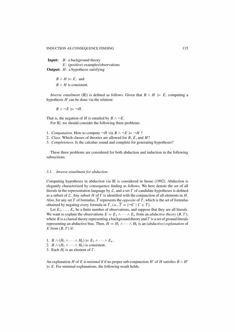
Input: B: a background theoryE : (positive) examples/observations

Output: H : a hypothesis satisfying

B ∧ H |= E, and

B ∧ H is consistent.

Inverse entailment (IE) is defined as follows. Given that B ∧ H |= E , computing ahypothesis H can be done via the relation:

B ∧ ¬E |= ¬H.

That is, the negation of H is entailed by B ∧ ¬E .For IE, we should consider the following three problems.

1. Computation. How to compute ¬H via B ∧ ¬E |= ¬H ?2. Class. Which classes of theories are allowed for B, E , and H?3. Completeness. Is the calculus sound and complete for generating hypotheses?

These three problems are considered for both abduction and induction in the followingsubsections.

3.1. Inverse entailment for abduction

Computing hypotheses in abduction via IE is considered in Inoue (1992). Abduction iselegantly characterized by consequence finding as follows. We here denote the set of allliterals in the representation language by L, and a set � of candidate hypotheses is definedas a subset of L. Any subset H of � is identified with the conjunction of all elements in H .Also, for any set T of formulas, T represents the opposite of T , which is the set of formulasobtained by negating every formula in T , i.e., T = {¬C | C ∈ T }.

Let E1, . . . , En be a finite number of observations, and suppose that they are all literals.We want to explain the observations E = E1 ∧ · · · ∧ En from an abductive theory (B, �),where B is a clausal theory representing a background theory and � is a set of ground literalsrepresenting an abductive bias. Then, H = H1 ∧ · · · ∧ Hk is an (abductive) explanation ofE from (B, �) if:

1. B ∧ (H1 ∧ · · · ∧ Hk) |= E1 ∧ · · · ∧ En ,

2. B ∧ (H1 ∧ · · · ∧ Hk) is consistent,3. Each Hi is an element of �.

An explanation H of E is minimal if if no proper sub-conjunction H ′ of H satisfies B ∧ H ′

|= E . For minimal explanations, the following result holds.

116 K. INOUE

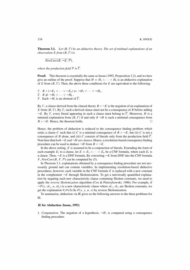
Theorem 3.1. Let (B, �) be an abductive theory. The set of minimal explanations of anobservation E from (B, �) is:

NewCarc(B, ¬E,P) ,

where the production field P is �.

Proof: This theorem is essentially the same as Inoue (1992, Proposition 3.2), and we heregive an outline of the proof. Suppose that H = H1 ∧ · · · ∧ Hk is an abductive explanationof E from (B, �). Then, the above three conditions for E are equivalent to the following:

1′. B ∧ (¬E1 ∨ · · · ∨ ¬En) |= ¬H1 ∨ · · · ∨ ¬Hk ,

2′. B �|= ¬H1 ∨ · · · ∨ ¬Hk ,

3′. Each ¬Hi is an element of �.

By 1′, a clause derived from the clausal theory B ∧ ¬E is the negation of an explanation ofE from (B, �). By 2′, such a derived clause must not be a consequence of B before adding¬E . By 3′, every literal appearing in such a clause must belong to �. Moreover, H is aminimal explanation from (B, �) if and only if ¬H is such a minimal consequence fromB ∧ ¬E . Hence, the theorem holds.

Hence, the problem of abduction is reduced to the consequence finding problem whichseeks a clause C such that (i) C is a minimal consequence of B ∧ ¬E , but (ii) C is not aconsequence of B alone, and (iii) C consists of literals only from the production field �.Note here that both ¬E and ¬H are clauses. Hence, a resolution-based consequence findingprocedure can be used to deduce ¬H from B ∧ ¬E .

In the above setting, E is assumed to be a conjunction of literals. Extending the form ofeach example Ei to a clause, let E = E1 ∧ · · · ∧ En be a CNF formula, where each Ei isa clause. Then, ¬E is a DNF formula. By converting ¬E from DNF into the CNF formulaF , NewCarc(B, F,P) can be computed by (5).

In Theorem 3.1, explanations obtained by a consequence finding procedure are not nec-essarily ground and can contain variables. In implementing resolution-based abductiveprocedures, however, each variable in the CNF formula E is replaced with a new constantin the complement ¬E through Skolemization. To get a universally quantified explana-tion by negating each new characteristic clause containing Skolem constants, we need toapply the reverse Skolemization algorithm (Cox & Pietrzykowski, 1986). For example, if¬P(x, sky, u, skv) is a new characteristic clause where sky, skv are Skolem constants, weget the explanation ∀y∀v∃x∃u P(x, y, u, v) by reverse Skolemization.

To summarize, abduction via IE gives us the following answers to the three problems forIE.

IE for Abduction (Inoue, 1992)

1. Computation. The negation of a hypothesis, ¬H , is computed using a consequencefinding procedure.


2. Class. In the basic setting, we consider

B: a full clausal theory (containing non-Horn clauses),E : a conjunction of (existentially-quantified) literals,H : a conjunction of literals (belonging to the abductive bias).

3. Completeness. For the above class, the IE calculus is sound and complete for computingabductive explanations.

3.2. Inverse entailment for induction

Computing hypotheses in induction via IE was first considered by Muggleton (1995) in theProgol system. Muggleton considered a Horn program for a background theory B, a singleHorn clause as an example E , and a single Horn clause as a hypothesis H . Even in thissetting, however, neither ¬E nor ¬H is a single clause. Moreover, both ¬E and ¬H containexistentially quantified variables. This means that a simple application of a resolution-based procedure is not sufficient to compute inductive hypothesis. Then, Muggleton (1995)introduced the bottom clause:

⊥(B, E) = {¬L | L is a literal and B ∧ ¬E |= L}, (7)

and a hypothesis H is constructed by generalizing a sub-clause of ⊥(B, E), i.e.,

H |= ⊥(B, E). (8)

Any hypothesis H obtained in this way is correct, that is, it satisfies B ∧ H |= E . Yamamoto(2000) used two special consequence finding procedures to implement IE in this way.However, Yamamoto (1997) also showed that this method is incomplete for finding inductivehypotheses (see Example 4.3 in this paper). Sufficient conditions for the completeness tohold have been investigated in Yamamoto (1997) and Furukawa (1997). See the details ofthese previous works in Section 6.

Hence, induction via IE by Muggleton (1995) can be summarized as follows.

IE for Induction (Muggleton, 1995)

1. Computation. The negation of a hypothesis, ¬H , is computed using consequence findingprocedures (Yamamoto, 2000).

2. Class. In the original setting, we consider

B: a Horn program,E : a Horn clause,H : a Horn clause.

3. Completeness. For the above class, the IE calculus is sound but incomplete for computinginductive hypotheses (Yamamoto, 1997).

In the next section, we introduce a new approach to IE called CF-Induction. Insteadof computing the bottom clause ⊥(B, E), CF-induction computes characteristic clauses

118 K. INOUE

of B ∧ ¬E , hence any resolution-based consequence finding procedure can be used. CF-induction includes all previous approaches to IE as special cases, in particular, includesabductive computation.

The specification of CF-induction is as follows. The details are given in Section 4.

CF-Induction1. Computation. A consequence finding procedure is used.2. Class. The most general class is considered:

B: a full clausal theory,E : a full clausal theory,H : a full clausal theory.

3. Completeness. The IE calculus is sound and complete for computing inductive hypothe-ses.

4. Induction as consequence finding

In this section, we characterize explanatory induction by consequence finding.

4.1. CF-induction

Suppose that we are given a background theory B and examples E , both of which are clausaltheories (or CNF) possibly containing non-Horn clauses. Recall that explanatory inductionseeks a clausal theory H such that:

B ∧ H |= E,

B ∧ H is consistent.

These two are equivalent to

B ∧ ¬E |= ¬H, (9)

B �|= ¬H. (10)

Like inverse entailment, we are interested in some formulas derived from B ∧ ¬E that arenot derived from B alone. Here, instead of the negation of the bottom clause ⊥(B, E) inMuggleton (1995), we consider some clausal theory CC(B, E) as a “bridge” formula U .Then, Eq. (9) can be written as

B ∧ ¬E |= CC(B, E), (11)

CC(B, E) |= ¬H. (12)

The latter (12) is also written as

H |= ¬CC(B, E). (13)


Also, by (10) and (12), we have

B �|= CC(B, E). (14)

By (11), CC(B, E) is obtained by computing the characteristic clauses of B ∧¬E becauseany other consequence of B ∧¬E belonging to P can be obtained by constructing a clausethat is subsumed by a characteristic clause. Hence,

Carc(B ∧ ¬E,P) |= CC(B, E), (15)

where the production fieldP = 〈 L, Cond 〉 is defined as a pair of a set L of literals reflectingan inductive bias in the complement form and a certain condition Cond. When no inductivebias is considered, P is just set to L, which is the set of all literals in the first-order language.The other requirement for CC(B, E) is Eq. (14), which is satisfied if at least one of theclauses in CC(B, E) is not a consequence of B; otherwise, CC(B, E) is entailed by B.This is realized by including a clause from NewCarc(B, ¬E,P) in CC(B, E).

In constructing a hypothesis H from the clausal theory CC(B, E), notice that ¬CC(B, E)is entailed by H in (13). Since ¬CC(B, E) is DNF, we convert it into the CNF formula F ,i.e.,

F ≡ ¬CC(B, E). (16)

Then, H is constructed as a clausal theory which entails F , i.e.,

H |= F. (17)

In ILP, there are several methods to compute a new clausal theory H which entails agiven clausal theory F . A procedure to construct such a more general clausal theory iscalled a generalizer (Yamamoto & Fronhofer, 2000) (see Section 4.2). Note that applyingan arbitrary generalizer to F may cause an inconsistency of H with B. To ensure thatB ∧ H is consistent, the clauses of H must keep those literals that are generalizations ofthe complement of at least one clause from NewCarc(B, ¬E,P).

Now, the whole algorithm to construct inductive hypotheses is as follows.

Definition 4.1. Let B and E be clausal theories. A clausal theory H is derived by a CF-induction from B and E if H is constructed as follows.

Step 1. Compute Carc(B ∧ ¬E,P);Step 2. Construct CC(B, E) = C1 ∧ · · · ∧ Cm , where each Ci is a clause satisfying the

conditions:

(a) Each Ci is an instance of a clause in Carc(B ∧ ¬E,P);(b) At least one Ci is an instance of a clause from NewCarc(B, ¬E,P);

Step 3. Convert ¬CC(B, E) into the CNF formula F ;Step 4. H is obtained by applying a generalizer to F under the constraint that B ∧ H is

consistent.

120 K. INOUE

Several remarks are necessary for the definition of CF-induction.

1. At Step 1, the number of characteristic clauses in Carc(B ∧ ¬E,P) may be large orinfinite in general. Hence, this step should be interleaved on demand with constructionof each Ci at Step 2 in practice.

2. At Step 2, a selected clause Ci in CC(B, E) can contain variables. In this case, eachvariable x in Ci is replaced with a Skolem constant skx in the complement ¬Ci at Step 3,in which x is interpreted as existentially quantified. Sometimes we need multiple Skolemconstants sk1

x , sk2x , · · · for each variable x of ¬Ci , depending on how many times Ci

is used in deriving ¬H from B ∧ ¬E . See 7 in the appendix for further details and anexample.

3. At Step 3, a DNF formula ¬CC(B, E) is converted to CNF. The complexity of thiscomputation is high, that is, in the class #P (Yamamoto & Fronhofer, 2000). Of course,we do not need this conversion if we allow a DNF hypothesis as H .

4.2. Generalizers

At Step 4 of CF-induction, we need a generalizer. The task of a generalizer is, given a CNFformula F , to find a CNF formula H such that

H |= F.

There are several methods to realize a generalizer. For example, the following techniquesare well-known, and can be jointly used as a generalizer.

• Reverse Skolemization (Cox & Pietrzykowski, 1986): Skolem constants/functions areconverted to existentially quantified variables.

• Anti-instantiation: ground terms are replaced with variables.• Anti-subsumption (dropping): some literals are dropped from a clause.• Strengthening (anti-weakening): some clauses are added. Yamamoto (2001) argued that

the application of anti-weakening might cause difficulties because any clausal theory F ′

that is a superset of F is derived as a correct hypothesis H with this operation. Hence,anti-weakening should be used in a restricted way so that H does not contain any clausewhich is not used to explain E .On the other hand, anti-weakening is necessary to assure the completeness of CF-induction (Theorem 4.4 in Section 4.4). For instance, any hypothesis which containredundant clauses can be obtained only by anti-weakening. This fact indicates that a realimplementation is incomplete if it avoids producing some redundant hypotheses.

• Inverse resolution (Muggleton & Buntine, 1988): the inverse of the resolution principleis applied. In some cases, this is reduced to the folding operation in logic program-ming (Pettorossi & Proietti, 1994). This operation is useful for introducing new predi-cates/literals not appearing in F .

• Least generalization (Plotkin, 1971): a least general generalization is constructed frommultiple clauses.


Note that if the “entailment” relation |= is replaced with the weaker “subsumption”relation in H |= F , the completeness in Theorem 4.1 (shown in Section 4.4) does notprecisely hold. When a hypothesis H such that H subsumes F is found, B ∧ H |= E doesnot necessarily hold, but it holds that H subsumes E relative to B in the sense of Plotkin(1971). See Yamamoto (1997) for details.

4.3. Examples

Example 4.1. For the introductory example shown in Section 1, B1 = human(s) andE1 = mortal(s). Then,

Carc(B1 ∧ ¬E1,L) = human(s) ∧ ¬mortal(s),

where ¬mortal(s) is the clause in NewCarc(B1, ¬E1,L). In this case, CC(B1, E1) is set toCarc(B1 ∧ ¬E1,L). Then,

F1 ≡ ¬CC(B1, E1) = ¬human(s) ∨ mortal(s).

By applying anti-instantiation to F1 with s/x , we get

H1 = (human(x) ⊃ mortal(x)).

Example 4.2. The following theory is a variant of an example in Buntine, 1988, and isoften used to illustrate how the bottom clause is used in inverse entailment (Yamamoto,1997, 2000, 2001). Consider

B2 = (cat(x) ⊃ pet(x)) ∧(small(x) ∧ fluffy(x) ∧ pet(x) ⊃ cuddly pet(x)),

E2 = (fluffy(x) ∧ cat(x) ⊃ cuddly pet(x)).

Then, the complement of E2 is

¬E2 = fluffy(skx) ∧ cat(skx) ∧ ¬cuddly pet(skx),

and NewCarc(B2, ¬E2,L) is

¬E2 ∧ pet(skx ) ∧ ¬small(skx ).

Let CC(B2, E2) = NewCarc(B2, ¬E2,L). In this case, F2 = ¬CC(B2, E2) is equivalentto ⊥(B2, E2). By applying reverse Skolemization (or anti-instantiation) to F2, we get thehypothesis:

H2 = (fluffy(x) ∧ cat(x) ∧ pet(x) ⊃ cuddly pet(x) ∨ small(x)).

122 K. INOUE

While in the above cited references the subclause of H2:

fluffy(x) ∧ cat(x) ⊃ small(x)

is often adopted as a definite clause, H2 is the most-specific hypothesis in the sense ofMuggleton (1995).

In Yamamoto (2001), the following hypothesis:

H ′2 = (pet(x) ⊃ dog(x)) ∧ (dog(x) ⊃ small(x))

is shown as another correct hypothesis if dog is a predicate symbol in the language. This isobtained if we take CC ′(B2, E2) = pet(skx )∧¬small(skx ). That is, F ′

2 = ¬CC ′(B2, E2) =(pet(skx ) ⊃ small(skx )). Then, H ′

2 is constructed by applying anti-instantiation and inverseresolution (or folding).

Example 4.3. This example (Yamamoto, 1997) illustrates the incompleteness of inverseentailment based on the bottom clause in Muggleton (1995). Consider the backgroundtheory and the example:

B3 = even(0) ∧ (¬odd(x) ∨ even(s(x))),

E3 = odd(s(s(s(0)))).

Then, Carc(B3 ∧ ¬E3,L) = B3 ∧ ¬E3. Suppose that CC(B3, E3) is chosen as:

even(0) ∧ (¬odd(s(0)) ∨ even(s(s(0)))) ∧ ¬odd(s(s(s(0)))),

where the second clause is an instance of the second clause in B3, and the third clausebelongs to NewCarc(B3, ¬E3,L). By converting ¬CC(B3, E3) into CNF, F3 consists ofthe clauses:

¬even(0) ∨ odd(s(0)) ∨ odd(s(s(s(0)))),

¬even(0) ∨ ¬even(s(s((0))) ∨ odd(s(s(s(0)))).

Considering the single clause:

H3 = ¬even(x) ∨ odd(s(x)),

H3 subsumes both clauses in F3, so is a hypothesis. There are many ways to compute H3

from F3. For example, by computing the least generalization of the two clauses in F3, weobtain the clause:

¬even(0) ∨ ¬even(x) ∨ odd(s(x)) ∨ odd(s(s(s(0)))).


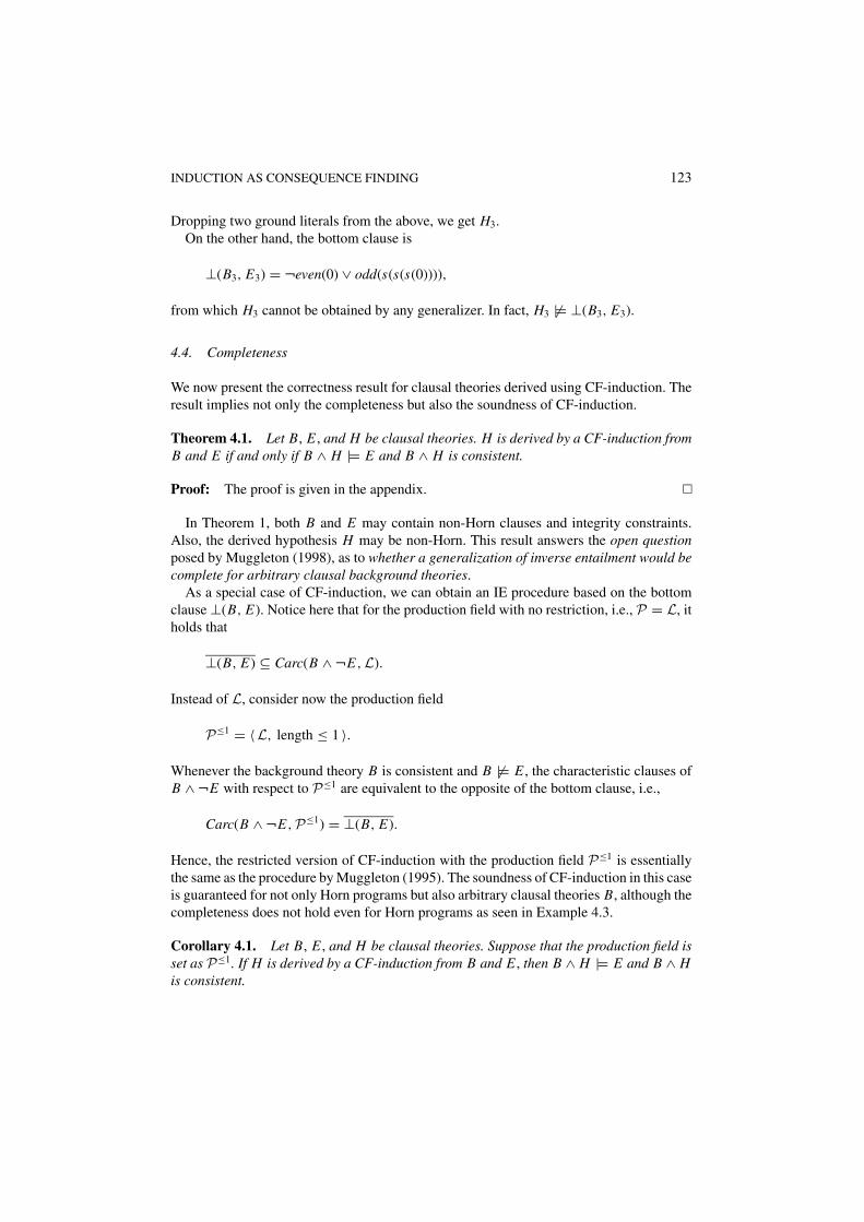
Dropping two ground literals from the above, we get H3.On the other hand, the bottom clause is

⊥(B3, E3) = ¬even(0) ∨ odd(s(s(s(0)))),

from which H3 cannot be obtained by any generalizer. In fact, H3 �|= ⊥(B3, E3).

4.4. Completeness

We now present the correctness result for clausal theories derived using CF-induction. Theresult implies not only the completeness but also the soundness of CF-induction.

Theorem 4.1. Let B, E , and H be clausal theories. H is derived by a CF-induction fromB and E if and only if B ∧ H |= E and B ∧ H is consistent.

Proof: The proof is given in the appendix.

In Theorem 1, both B and E may contain non-Horn clauses and integrity constraints.Also, the derived hypothesis H may be non-Horn. This result answers the open questionposed by Muggleton (1998), as to whether a generalization of inverse entailment would becomplete for arbitrary clausal background theories.

As a special case of CF-induction, we can obtain an IE procedure based on the bottomclause ⊥(B, E). Notice here that for the production field with no restriction, i.e., P = L, itholds that

⊥(B, E) ⊆ Carc(B ∧ ¬E,L).

Instead of L, consider now the production field

P≤1 = 〈L, length ≤ 1 〉.

Whenever the background theory B is consistent and B �|= E , the characteristic clauses ofB ∧ ¬E with respect to P≤1 are equivalent to the opposite of the bottom clause, i.e.,

Carc(B ∧ ¬E,P≤1) = ⊥(B, E).

Hence, the restricted version of CF-induction with the production field P≤1 is essentiallythe same as the procedure by Muggleton (1995). The soundness of CF-induction in this caseis guaranteed for not only Horn programs but also arbitrary clausal theories B, although thecompleteness does not hold even for Horn programs as seen in Example 4.3.

Corollary 4.1. Let B, E , and H be clausal theories. Suppose that the production field isset as P≤1. If H is derived by a CF-induction from B and E , then B ∧ H |= E and B ∧ His consistent.

124 K. INOUE

4.5. Negative examples

So far, we have not considered negative examples in CF-induction. To avoid over-generaliza-tion, it is common for an ILP system to use negative examples as well as positive ones. ForCF-induction, negative examples can also be incorporated as follows.

Suppose that B, E+, and E− are a background theory, positive examples, and a nega-tive example, respectively. Here, we assume that there exists only one negative example,but extending the case to multiple negative examples is possible. The task of explanatoryinduction in this case is to compute a hypothesis H satisfying both

B ∧ H |= E+

and

B ∧ H �|= E−.

Here, the negative example can be used to reduce the number of possible choices forCC(B, E+), which contributes toward increasing the efficiency of CF-induction as follows.Instead of (10), we now have

B ∧ ¬E− �|= ¬H,

and the relation (14) is replaced with

B ∧ ¬E− �|= CC(B, E+).

Hence, it holds that

Carc(B ∧ ¬E−,P) �|= CC(B, E+).

Then, at Step 2(b) of CF-induction, an instance of a clause from Carc(B ∧ ¬E+,P) −Carc(B ∧ ¬E−,P) must be selected in CC(B, E+). Moreover, at Step 4, H must beconstructed so that B ∧ H �|= E−.

4.6. Implementation

An incomplete version of CF-induction has been implemented in Java. The incomplete-ness of such a procedure is due to the incompleteness of generalizers. In particular, anti-weakening (clause addition) cannot be realized completely, but this is not practically bad be-cause increasing clauses in H results in a redundant hypothesis in general (see Section 4.2).As a consequence finding procedure, we have realized a tableaux version of SOL resolution(Iwanuma, Inoue, & Satoh, 2000). After computing Carc(B ∧ ¬E,P), the selection ofCC(B, E) is guided by a menu, in which a user choose clauses from Carc(B ∧ ¬E,P).


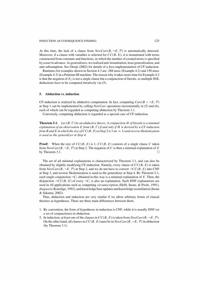
At this time, the lack of a clause from NewCarc(B, ¬E,P) is automatically detected.Moreover, if a clause with variables is selected for CC(B, E), it is instantiated with termsconstructed from constants and functions, in which the number of created terms is specifiedby a user in advance. As generalizers, we realized anti-instantiation, least generalization, andanti-subsumption. See Otsuji (2002) for details of a Java implementation of CF-induction.

Runtimes for examples shown in Section 4.3 are: 288 msec (Example 4.2) and 150 msec(Example 4.3) in a Pentium III machine. The reason why it takes more time for Example 4.2is that the negation of E2 is not a single clause but a conjunction of literals, so multiple SOLdeductions have to be computed iteratively via (5).

5. Abduction vs. induction

CF-induction is realized by abductive computation. In fact, computing Carc(B ∧ ¬E,P)at Step 1 can be implemented by calling NewCarc operations incrementally in (5) and (6),each of which can be regarded as computing abduction by Theorem 3.1.

Conversely, computing abduction is regarded as a special case of CF-induction.

Theorem 5.1. Let (B, �) be an abductive theory. A conjunction H of literals is a minimalexplanation of an observation E from (B, �) if and only if H is derived by a CF-inductionfrom B and E in which the size of CC(B, E) at Step 2 is 1 (m = 1) and reverse Skolemizationis used as the generalizer at Step 4.

Proof: When the size of CC(B, E) is 1, CC(B, E) consists of a single clause C takenfrom NewCarc(B, ¬E,P) at Step 2. The negation of C is then a minimal explanation of Eby Theorem 3.1.

The set of all minimal explanations is characterized by Theorem 3.1, and can also beobtained by slightly modifying CF-induction. Namely, every clause of CC(B, E) is takenfrom NewCarc(B, ¬E,P) at Step 2, and we do not have to convert ¬CC(B, E) into CNFat Step 3, and reverse Skolemization is used as the generalizer at Step 4. By Theorem 5.1,each single conjunction ¬Ci obtained in this way is a minimal explanation of E . Then, thedisjunction ¬CC(B, E) of every ¬Ci is also an explanation. Such DNF explanations areused in AI applications such as computing circumscription (Helft, Inoue, & Poole, 1991),diagnosis (Konolige, 1992), and knowledge base updates and knowledge assimilation (Inoue& Sakama, 2002).

Thus, abduction and induction are very similar if we allow arbitrary forms of clausaltheories as hypotheses. There are three main differences between them.

1. By convention, the form of hypotheses in induction is CNF, while it is usually DNF (ora set of conjunctions) in abduction.

2. In induction, at least one of the clauses in CC(B, E) is taken from NewCarc(B, ¬E,P).On the other hand, all clauses in CC(B, E) must be in NewCarc(B, ¬E,P) in abduction(by Theorem 3.1).

126 K. INOUE

3. Reverse Skolemization is solely used as a generalizer in abduction, while other gen-eralizers can be used in induction. In particular, when anti-weakening is allowed asa generalizer, an obtained hypothesis is not necessarily minimal in induction, whileminimal explanations are usually preferred in abduction.

No other difference exists between abduction and induction as long as their implementa-tion is concerned in the context of consequence finding. The next example illustrates thesimilarity between induction and abduction.

Example 5.1. (Yamamoto & Fronhofer, 2000). Let

B4 = (dog(x) ∧ small(x) ⊃ pet(x)),

E4 = pet(c).

be the background theory and the example. Then,

NewCarc(B4, ¬E4,L) = ¬pet(c) ∧ (¬dog(c) ∨ ¬small(c)).

Now, put CC(B4, E4) = NewCarc(B4, ¬E4,L). Then,

¬CC(B4, E4) = pet(c) ∨ (dog(c) ∧ small(c)),

which is exactly the same as the minimal abductive explanations. Converting ¬CC(B4, E4)into CNF, we have

F4 = (dog(c) ∨ pet(c)) ∧ (small(c) ∨ pet(c)).

By applying anti-instantiation, we get the clausal theory:

H4 = (dog(x) ∨ pet(x)) ∧ (small(x) ∨ pet(x)).

On the other hand, the next example shows the main difference between abduction andinduction, which is the second one in the above differences: all clauses in CC(B, E)are taken from NewCarc(B, ¬E,P) in abduction, while it is not the case in induction.Namely, induction often utilizes consequences of B before adding ¬E in the constructionof CC(B, E). This operation is essential to associate observations E with the backgroundtheory B in induction. Abduction, on the other hand, does not need such consequences ofB because they are redundant in virtue of the minimality of explanations. This differencealso reflects Peirce’s theory of induction and abduction (Peirce, 1932): induction infers arule (i.e., hypothesis) A ⊃ C from a case (i.e., background theory) A and a result (i.e.,example/observation) C , while abduction infers a case A from a rule A ⊃ C and a result C .


Example 5.2. (Muggleton, 1995). Let us consider the background theory and the example:

B5 = white(swan1), E5 = ¬black(swan1).

Then, NewCarc(B5, ¬E5,L) = ¬E5 = black(swan1). Hence, ¬black(swan1) is theunique minimal abductive explanation of E5. In induction, on the other hand, let

CC(B5, E5) = white(swan1) ∧ black(swan1),

in which the first conjunct is the clause of B5. By anti-instantiating F5 = ¬CC(B5, E5),we can learn the integrity constraint:

H5 = ¬white(x) ∨ ¬black(x).

6. Related work

6.1. Previous work on inverse entailment

CF-induction is obviously influenced by previous work on inverse entailment (IE). As shownin Section 3.2, the original IE (Muggleton, 1995) allows Horn clauses for B and a singleHorn clause for each of H and E . Even in this setting, however, IE based on ⊥(B, E) isincomplete for finding H such that B ∧ H |= E (Yamamoto, 1997). Furukawa et al. (1997)consider a sufficient condition for IE to be complete, which restricts the class of logicprograms to a proper subset of the Horn programs. Muggleton (1998) considers an enlargedbottom set to make IE complete in the class of Horn programs, but the revised method isunsound. Furukawa (1998) also proposes a complete algorithm, but it is relatively complex.Yamamoto (2000) shows that a variant of SOL resolution can be used to implement IE basedon ⊥(B, E). However, he computes positive and negative parts in ⊥(B, E) separately, whereSOL resolution is used only for computing positive literals. Muggleton and Bryant (2000)suggest the use of PTTP (Stickel, 1988) for implementing theory completion using IE,which seems inefficient since PTTP is not a consequence finding procedure but a theoremprover. Compared with these previous works, CF-induction proposed in this paper is simple,yet sound and complete for finding hypotheses from not only Horn programs but also fullclausal theories. Instead of the bottom clause, CF-induction uses the characteristic clauses,which strictly include the unit clauses in ⊥(B, E).

6.2. Yamamoto and Fronhofer

Yamamoto and Fronhofer (2000) first extend IE to allow for full clausal theories for B andE , and introduce the notion of a residue hypothesis for a set of ground instances of B ∧¬E .A residue hypothesis is computed from the ground instances T of B ∧ ¬E by:

1. Select a finite set (i.e., conjunction) S of ground clauses from T ;

128 K. INOUE

2. Convert ¬S into the CNF formula R;3. Remove all tautologies from R.

An inductive hypothesis H is then computed by applying a generalizer to a residue hypoth-esis.

A residue hypothesis can be computed using Bibel’s Connection method (Bibel, 1993),and the constructed CNF formula R corresponds to the enumeration of all paths in thematrix of clauses S. By contrast, CF-induction is realized by a resolution-based consequencefinding procedure, which naturally extends most previous work on IE, and can easily handlenon-ground clauses.

Compared with the procedure by Yamamoto and Fronhofer, a merit of CF-induction liesin the existence of a production field P , which can be used to guide and restrict derivationsof clauses by reflecting an inductive bias. Usually, we are given some inductive bias forinductive problems. For example, the production field P≤1 in Section 4.4 guides derivationsof a consequence finding procedure to produce unit clauses only. Also, Progol (Muggleton,1995) uses mode declarations to constrain search for H which subsumes ⊥(B, E). It isunclear how to incorporate inductive biases in the procedure of Yamamoto and Fronhofer(2000).

Note that the consistency of a residue hypothesis is not always guaranteed. Although notmentioned in Yamamoto and Fronhofer (2000), the consistency is assured if instances of¬E are selected within S from the ground instances T of B ∧ ¬E , which is similar to ourincorporation of NewCarc(B, ¬E,P) into CC(B, E).

Finally, residue hypotheses are relatively longer and more complex than hypothesesconstructed by CF-induction, and require more efforts for a generalizer to construct a finalinductive hypothesis H .

Example 6.1. Suppose that we are given the background theory and an example as:

B6 = (a ∨ b) ∧ (a ⊃ c) ∧ (b ⊃ c) ∧ (d ⊃ g),

E6 = g.

Then,

NewCarc(B6, ¬E6,L) = ¬d ∧ ¬g,

Carc(B6 ∧ ¬E6,L) = NewCarc(B6, ¬E6,L) ∧ (a ∨ b) ∧ c.

If we put CC(B6, E6) = Carc(B6 ∧ ¬E6,L), we get a hypothesis:

H6 = (a ∧ c ⊃ d ∨ g) ∧ (b ∧ c ⊃ d ∨ g).

Alternatively, suppose we take another bridge as

CC ′(B6, E6) = c ∧ ¬d.


Then,

F ′6 = ¬CC ′(B6, E6) = (c ⊃ d).

This formula F ′6 is taken as an inductive hypothesis H ′

6 without applying any generalizer.On the other hand, it is not easy to obtain H ′

6 = (c ⊃ d) using Yamamoto and Fronhofer(2000) method. Firstly, all clauses of B6 ∧ ¬E6 are necessary to construct H ′

6. Then, theresidue hypothesis for B6 ∧ ¬E6 is

(a ∧ c ⊃ b ∨ d ∨ g) ∧ (a ∧ c ⊃ d ∨ g)

∧ (b ∧ c ⊃ a ∨ d ∨ g) ∧ (b ∧ c ⊃ d ∨ g)

In the above formula, the first and the third clauses are subsumed by the second and fourthclauses, respectively, and are redundant. After removing them, take the least generalizationof (a ∧ c ⊃ d ∨ g) and (b ∧ c ⊃ d ∨ g), which is (c ⊃ d ∨ g). Finally, g is dropped fromthis clause to construct (c ⊃ d). Hence, subsumption tests must be used for simplifyingresidue hypotheses. In CF-induction, the notion of subsumption tests is already implicit inthe notion of characteristic clauses.

7. Conclusion and future work

In this paper, we have defined a general resolution-based method to construct inductivehypotheses from full clausal theories. We put emphasis on finding a sound and completemethod for inverse entailment in full clausal theories, which was a long-standing openproblem in ILP. To this problem, we have suggested a simple yet powerful solution: CF-induction. Salient features of CF-induction are summarized as follows.

• CF-induction is sound and complete for finding hypotheses from full clausal theories.• CF-induction performs induction via consequence finding, which enables us to generate

inductive hypotheses in a logically principled way based on the resolution principle.• CF-induction can be implemented with existing systematic consequence finding proce-

dures such as SOL resolution (Inoue, 1992) and SFK resolution (del Val, 1999).• CF-induction includes, as special cases, computing abductive explanations and the bot-

tom clause. Also, a restriction on the hypothesis vocabulary can easily be realized byspecifying a production field.

We also clarified the similarity and difference between abduction and induction in thecontext of consequence finding.

CF-induction by Definition 4.1 computes the characteristic clauses Carc(B ∧ ¬E,P),selects CC(B, E) to be a set of instances of Carc(B∧¬E,P), and then applies a generalizerto the complement of CC(B, E) to obtain H . There are two choice points in this method: thechoice of CC(B, E), and the choice of the generalizer. Currently, these two choice pointscannot be combined into one. However, an open question is whether or when it is possible

130 K. INOUE

to construct a single bridge formula U such that any H can be derived in the complementform from U using a generalizer. A simple method for such an ultimate bridge would beto include all clauses from Carc(B ∧ ¬E,P) into CC(B, E). However, this only workswhen (the instances of) Carc(B ∧¬E,P) is finite, and even in the finite case, a generalizershould work very hard! In other words, a heavy work load of a generalizer is reduced if anappropriate choice is made in the selection of CC(B, E).

A prototype system of CF-induction has been implemented in Java, but efficient imple-mentation of CF-induction is an important future work. In particular, an intelligent selectionof CC(B, E) from Carc(B ∧ ¬E,P) needs to be addressed. To remove the manual inter-vention in this step from the system, one can perform a search in the space of subsets ofCarc(B ∧ ¬E,P) or the space of possible instantiations of the clauses. In such a case, weneed heuristics for guiding searches, e.g., compression and the description length. More-over, testing the (extended) system with intelligent search on large and practical problemsof learning from positive examples is necessary in the future, as for those examples usedin Muggleton (2001). Learning from both positive and negative examples should also beautomated with search in the framework of CF-induction. These extensions are necessaryfor the algorithm of CF-induction to construct a practical ILP system. However, we shouldagain put emphasis on the completeness of CF-induction in extended systems. Making anILP system complete is worthwhile to discover an interesting hypothesis even if it takesmuch time.

Finally, there exist formalizations of induction other than explanatory induction in theliterature on ILP, such as learning from interpretations (or satisfiability) (De Raedt, 1997),and descriptive induction (Helft, 1989; Lachiche, 2000). De Raedt (1997) proposes a trans-lation of learning from interpretations into learning from entailment, but the method requiresnegative examples. Lachiche (2000) discusses various forms of descriptive induction, whichcan also be characterized by deduction from completed theories. The precise relationshipsbetween these different formalisms and consequence finding need to be addressed in thefuture.

Appendix A. Proof of Theorem 3.1

We prove the correctness of CF-induction by giving its soundness and completeness. LetB, E and H be clausal theories. Section 7 shows that for any H derived by a CF-inductionfrom B and E , it holds that B ∧ H |= E and B ∧ H is consistent. Section 7 shows theconverse, that is, if B ∧ H |= E and B ∧ H is consistent then H is derived by a CF-inductionfrom B and E .

In the following, we assume the language LH for all hypotheses H ’s. Usually, LH isgiven as the set of all clauses constructed from the first-order language, but we can restrictthe form of hypotheses by considering an inductive bias with a subset of literals/predicates.The following proofs can be applied to the case with an inductive bias. In this case, theliterals specified in the production field P are set to the opposite of LH . When LH is the setof all clauses, P is given as L. Note that a length restriction in a production field cannot beused to assure the completeness (e.g., P≤1 in Section 4.4). We also assume the existence ofa sound and complete generalizer at Step 4 of a CF-induction.


A.1 Soundness of CF-induction

Let H be a hypothesis obtained by a CF-induction from B and E . By the definition ofa CF-induction, there is a CNF formula CC(B, E) = C1 ∧ · · · ∧ Cm such that [a] H isobtained by applying a generalizer to the CNF representation of ¬CC(B, E); [b] every Ci

(i = 1, . . . , m) is an instance of a clause from Carc(B ∧ ¬E,P); and [c] there is a C j

(1 ≤ j ≤ m) that is an instance of a clause from NewCarc(B, ¬E,P). By [b], for any Ci

(i = 1, . . . , m), there is a clause Di ∈ Carc(B ∧ ¬E,P) such that B ∧ ¬E |= Di andDi |= Ci . Obviously, it holds that B ∧¬E |= Ci . Also, by [c], it holds that B �|= C j . Hence,

B ∧ ¬E |= C1 ∧ · · · ∧ Cm and B �|= C1 ∧ · · · ∧ Cm .

Now, let

F ≡ ¬CC(B, E) ≡ ¬C1 ∨ · · · ∨ ¬Cm .

Then,

B ∧ ¬E |= ¬F and B �|= ¬F,

which are equivalent to

B ∧ F |= E and B ∧ F is consistent.

Finally, H |= F holds by [a], which implies that B ∧ H |= E . The condition that B ∧ H isconsistent is included in Step 4 of a CF-induction.

A.2 Completeness of CF-induction

Suppose that B ∧ H |= E and B ∧ H is consistent. Then, B ∧ ¬E |= ¬H and B �|= ¬H .Since H belongs to LH that is the opposite of the literals in P , ¬H belongs to P . Bythe definition of the characteristic clauses, any consequence of B ∧ ¬E belonging to P issubsumed by a clause in Carc(B ∧ ¬E,P). Therefore,

Carc(B ∧ ¬E,P) |= ¬H.

Hence, Carc(B ∧ ¬E,P) ∧ H is unsatisfiable.Now, there are two ways to prove the completeness of CF-induction: one uses Herbrand’s

theorem, and the other uses the compactness theorem.

Theorem A.1 (Herbrand’s Theorem). A set of clauses � is unsatisfiable if and only if afinite set of ground instances of clauses of � is unsatisfiable.

132 K. INOUE

Theorem A.2 (Compactness). Let � be a set of clauses. If all finite subsets of � issatisfiable, then so is �. Equivalently, if � is unsatisfiable then a finite subset of � isunsatisfiable.

A.2.1 [A] Using Herbrand’s theorem. There is a finite set S of ground instances ofclauses from Carc(B ∧ ¬E,P) such that S ∧ H is unsatisfiable. This set S can actually beconstructed by a CF-induction. In fact, we can set S as CC(B, E). In other words, let usconstruct CC(B, E) = C1 ∧ · · · ∧ Cm at Step 2 of a CF-induction such that

(a) each Ci (i = 1, . . . , m) is a ground instance of a clause from Carc(B ∧ ¬E,P),(b) C1 ∧ · · · ∧ Cm ∧ H is unsatisfiable.

Then, there is a C j (1 ≤ j ≤ m) that is a ground instance of a clause from NewCarc(B, ¬E,

P) (for this, see the discussion below Eq. (15) in Section 4). Finally, at Steps 3 and 4, H can beobtained by applying a generalizer (including anti-instantiation) to the CNF representationof ¬CC(B, E).

A.2.2 [B] Using the compactness theorem. There is a finite subset S of Carc(B∧¬E,P)such that S ∧ H is unsatisfiable. In this case, S can also be constructed at Step 2 of a CF-induction as CC(B, E) = C1 ∧ · · · ∧ Cm , where

(a) every Ci (i = 1, . . . , m) is a variant of a clause from Carc(B ∧ ¬E,P), and(b) C1 ∧ · · · ∧ Cm ∧ H is unsatisfiable.

Then, there is a C j (1 ≤ j ≤ m) that is a variant of a clause in NewCarc(B, ¬E,P) as inthe proof of [A]. In this case, however, we have to take care of variables in Ci ’s. Taking thecomplement of a Ci , each variable x in Ci becomes a Skolem constant skx in ¬Ci , in whichx is interpreted as existentially quantified. Sometimes we need multiple “copies” of ¬Ci in¬CC(B, E) using different constants like sk1

x , sk2x , etc, depending on how many times Ci

is used to derive ¬H from B ∧ ¬E . Then, at Steps 3 and 4, H can be obtained by applyinga generalizer to the CNF representation of ¬CC(B, E).

Example A.1. We now verify the completeness proof [B] by applying it to a variant ofExample 4.3 from Yamamoto and Fronhofer (2000, Example 2), while the proof [A] caneasily be checked in Example 4.3. Let us consider the background theory and the example:

B7 = even(0) ∧ (¬odd(x) ∨ even(s(x))),

E7 = odd(s5(0)),

where s1(0) = s(0) and sn(0) = s(sn−1(0)) for n > 1. This time, we choose a non-groundcharacteristic clause as

CC(B7, E7) = even(0) ∧ (¬odd(x) ∨ even(s(x))) ∧ ¬odd(s5(0)).


By making two copies of ∃x(odd(x) ∧ ¬even(s(x))), the complement of CC(B7, E7) be-comes

(¬even(0) ∨ odd(sk1x

) ∨ odd(sk2

x

) ∨ odd(s5(0)))

∧ (¬even(0) ∨ odd(sk1

x

) ∨ ¬even(s(sk2

x

)) ∨ odd(s5(0)))

∧ (¬even(0) ∨ ¬even(s(sk1

x

)) ∨ odd(sk2

x

) ∨ odd(s5(0)))

∧ (¬even(0) ∨ ¬even(s(sk1

x

)) ∨ ¬even(s(sk2

x

)) ∨ odd(s5(0))),

which represents

∃y∃z [ (¬even(0) ∨ odd(y) ∨ odd(z) ∨ odd(s5(0))) ∧(¬even(0) ∨ odd(y) ∨ ¬even(s(z)) ∨ odd(s5(0))) ∧(¬even(0) ∨ ¬even(s(y)) ∨ odd(z) ∨ odd(s5(0))) ∧(¬even(0) ∨ ¬even(s(y)) ∨ ¬even(s(z)) ∨ odd(s5(0))) ].

The hypothesis

H7 = ¬even(x) ∨ odd(s(x))

entails ¬CC(B7, E7). To see this, take the substitution {y/s(0), z/s3(0)} in the above for-mula. Then, H7 subsumes each clause in

(¬even(0) ∨ odd(s(0)))

∧ (¬even(s2(0)) ∨ odd(s3(0)))

∧ (¬even(s4(0)) ∨ odd(s5(0))),

and thus entails ¬CC(B7, E7).

Acknowledgments

In 1995, Koichi Furukawa first suggested me to use a consequence finding procedure forcomputing inverse entailment. In 1997, Akihiro Yamamoto succeeded in realizing such anattempt for Horn programs. I am indebted to them for their previous works and stimulativediscussions on improvement of IE calculi. I would like to thank reviewers for this paperand my ILP’01 paper for their helpful comments. I am grateful to Kanako Otsuji, Yoshi-taka Yamamoto, and Hidetomo Nabeshima for their efforts at implementing CF-induction.Thanks also for useful discussions and comments on the topics in this paper with LaurenceCholvy, Philip Reiser, Haruka Saito, and Hiromasa Haneda.

Note

1. A production field P is stable if, for any two clauses C and D such that C subsumes D, D belongs to P onlyif C belongs to P .

134 K. INOUE

References

Bibel, W. (1998). Deduction: Automated logic. Academic Press.Buntine, W. (1988). Generalized subsumption and its applications to induction and redundancy. Artificial Intelli-

gence, 36, 149–176.Cox, P. T., & Pietrzykowski, T. (1986). Causes for events: their computation and applications. In Proceedings of

the Eighth International Conference on Automated Deduction (pp. 608–621). LNCS 230, Springer.De Raedt, L. (1997). Logical settings for concept-learning. Artificial Intelligence, 95, 187–201.del Val, A. (1999). A new method for consequence finding and compilation in restricted languages. In Proceedings

of AAAI-99 (pp. 259–264). AAAI Press.Dimopoulos, Y., & Kakas, A. (1996). Abduction and inductive learning. In L. De Raedt (Ed.), Advances in

inductive logic programming. IOS Press.Flach, P. A., & Kakas, A. C. (Eds.). (2000). Abduction and induction: Essays on their relation and integration.

Kluwer.Furukawa, K., Murakami, T., Ueno, K., Ozaki, T., & K. Shimazu. (1997). On a sufficient condition for

the existence of most specific hypothesis in Progol. In N. Lavrac, & S. Dzeroski (Eds.), Proceed-ings of the Seventh International Workshop on Inductive Logic Programming (pp. 157–164). LNAI 1297,Springer.

Furukawa, K. (1998). On the completion of the most specific hypothesis computation in inverse entailment formutual recursion. In Proceedings of Discovery Science ’98 (pp. 315–325). LNAI 1532, Springer.

Gregoire, E., & Saıs, L. (1996). Inductive reasoning is sometimes deductive. In Proceedings of ECAI-96 Workshopon Abductive and Inductive Reasoning.

Helft, N. (1989). Induction as nonmonotonic inference. In R.J. Brachman, H.J. Levesque, & R. Reiter (Eds.),Proceedings of the First International Conference on Principles of Knowledge Representation and Reasoning(pp. 149–156). Morgan Kaufmann.

Helft, N., Inoue, K., & Poole, D. (1991). Query answering in circumscription. In Proceedings of IJCAI-91(pp. 426–431). Morgan Kaufmann.

Inoue, K. (1992). Linear resolution for consequence finding. Artificial Intelligence, 56, 301–353.Inoue, K. (2001). Induction, abduction, and consequence-finding. In C. Rouveirol, & M. Sebag (Eds.), Pro-

ceedings of the Eleventh International Conference on Inductive Logic Programming (pp. 65–79). LNAI 2157,Springer.

Inoue, K. (2002). Automated abduction. In A. Kakas, & F. Sadri (Eds.), Computational Logic: From LogicProgramming into the Future—In Honour of Bob Kowalski (Part II). LNAI 2408, Springer.

Inoue, K., & C. Sakama. (2002). Disjunctive explanations. In P. Stuckey (Ed.), Proceedings of the SeventeenthInternational Conference on Logic Programming (pp. 317–332), LNCS 2401, Springer.

Iwanuma, K., Inoue, K., & Satoh, K. (2000). Completeness of pruning methods for consequence finding procedureSOL. In P. Baumgartner, & H. Zhang (Eds.), Proceedings of the Third International Workshop on First-OrderTheorem Proving (pp. 89–100).

Konolige, K. (1992). Abduction versus closure in causal theories. Artificial Intelligence, 53, 255–272.Lachiche, N. (2000). Abduction and induction from a non-monotonic reasoning perspective. In P.A. Flach, &

A.C. Kakas (Eds.), Abduction and induction: Essays on their relation and integration. Kluwer.Lee, C. T. (1967). A completeness theorem and computer program for finding theorems derivable from given

axioms. Ph.D. thesis, Department of Electrical Engineering and Computer Science, University of California,Berkeley, CA.

Marquis, P. (2000). Consequence finding algorithms. In D. M. Gabbay & P. Smets (Eds.), Handbook for defeasiblereasoning and uncertain management systems (vol. 5). Kluwer Academic.

Muggleton, S. (1995). Inverse entailment and Progol. New Generation Computing, 13, 245–286.Muggleton, S. (1998). Completing inverse entailment. In D. Page (Ed.), Proceedings of the Eighth International

Conference on Inductive Logic Programming (pp. 245–249). LNAI 1446, Springer.Muggleton, S. (2001). Learning from positive data. Machine Learning, to appear.Muggleton, S., & Bryant, C. (2000). Theory completion and inverse entailment. In J. Cussens, & A. Frisch

(Eds.), Proceedings of the Tenth International Conference on Inductive Logic Programming (pp. 130–146).LNAI 1866, Springer.


Muggleton, S., & Buntine, W. (1988). Machine invention of first-order predicates by inverting resolution. InProceedings of the Fifth International Conference on Machine Learning (pp. 339–352). Morgan Kaufmann.

Nienhuys-Cheng, S. H., & de Wolf, R. (1997). Foundations of inductive logic programming. LNAI 1228, Springer.Otsuji, K. (2002). Research on implementation of CF-induction using SOL resolution. Graduation Thesis,

Department of Electrical and Electronics Engineering, Kobe University.Peirce, C. S. (1932). Elements of logic. In C. Hartshorne, & P. Weiss (Eds.), Collected papers of Charles Sanders

Peirce (vol. II). Cambridge, MA: Harvard University Press.Pettorossi, A., & Proietti, M. (1994). Transformation of logic programs: foundations and techniques. Journal of

Logic Programming, 19 & 20, 261–320.Plotkin, G. D. (1971). A further note on inductive generalization. In B. Meltzer, & D. Michie (Eds.), Machine

intelligence (vol. 6). Edinburgh University Press.Stickel, M. E. (1988). A Prolog technology theorem prover: implementation by an extended Prolog compiler.

Journal of Automated Reasoning, 4, 353–380.Yamamoto, A. (1997). Which hypotheses can be found with inverse entailment? In N. Lavrac, & S. Dzeroski

(Eds.), Proceedings of the Seventh International Workshop on Inductive Logic Programming (pp. 296–308).LNAI 1297, Springer.

Yamamoto, A. (2000). Using abduction for induction based on bottom generalization. In Flach, & Kakas, 2000,Abduction and induction: Essays on their relation and integration. Kluwer.

Yamamoto, A. (2002). Hypothesis finding based on upward refinement of residue hypotheses. TheoreticalComputer Science, to appear.

Yamamoto, A., & Fronhofer, B. (2000). Hypotheses finding via residue hypotheses with the resolution principle.In Proceedings of the Eleventh International Conference on Algorithmic Learning Theory (pp. 156–165). LNAI1968, Springer.

Received April 29, 2002Revised March 31, 2003Accepted July 25, 2003Final manuscript November 5, 2003

induction as consequence finding - rd.springer.commach.0000023149.7212… · based on inverse...

Documents