individual speed variance in traffic flow: analysis of … speed variance in traffic flow: analysis...

Individual speed variance in traffic flow: analysis

of Bay Area radar measurements

Sebastien Blandin1, Amir Salam2, Alex Bayen3

Submitted For Publication

91th Annual Meeting of the Transportation Research Board

August 1st, 2011

Word Count:

Number of words: 4664

Number of figures: 9 (250 words each)

Number of tables: 2 (250 words each)

Total: 7414

1 Corresponding Author, PhD student, Systems Engineering, Department of Civil and Environmental

Engineering, University of California, Berkeley, 621 Sutardja Dai Hall, Berkeley, CA, 94720-1764, USA. Email:

[email protected].

2 Master’s student, Transportation Engineering, Department of Civil and Environmental Engineering,

University of California, Berkeley, CA, 94720-1720, USA. Email: [email protected].

3 Associate Professor, Systems Engineering, Department of Electrical Engineering and Computer Sciences, Department of Civil and Environmental Engineering, University of California, Berkeley, 642 Sutardja Dai Hall, Berkeley, CA, 94720-1764, USA. Email: [email protected].

TRB 2012 Annual Meeting Paper revised from original submittal.

Abstract 1

2

The recent increase of mobile devices able to measure individual vehicles speed and 3

position with improved accuracy brings new opportunities to traffic engineers. The large 4

amount of individual probe measurements allows the study of phenomena previously 5

unobservable with conventional sensing technologies, and the design of novel traffic 6

monitoring and control strategies. However, challenges inherent to the use of speed and 7

location data arise. One of the main challenges of measurements collected from individual 8

vehicles lies in their ability to provide relevant information on the macroscopic properties 9

of traffic flow. According to the classical triangular fundamental diagram, the relation 10

between speed and flow can be inversed in the congestion phase but not in the 11

uncongested phase. In the latter, the flow of vehicles cannot be retrieved from the speed of 12

vehicles, assumed to be constant. This article proposes to investigate the nature of the 13

relationship between flow and speed from joint measurements from radar data. Two 14

different regression methods are proposed in this article to estimate traffic flow based on 15

individual speed measurements: regression of flow on speed and regression of flow on 16

speed variance. The respective performance of these two methods during specific traffic 17

periods is assessed, and recommendations on their relative strengths are provided. This 18

empirical study is conducted using 112 NAVTEQ radars [1] measuring speed and flow on 19

highways in the San Francisco Bay area, California. 20


1

I. Introduction 1

The recent years have witnessed an unprecedented growth in the number of traffic data 2

sources from connected mobile devices such as cell phones or cellular devices and 3

embedded GPS. In contrast to conventional loop detectors which output counts of vehicles 4

and occupancies (i.e. flows) that in turn can be used to estimate velocities, these new 5

widely spread sources only provide velocity and location information. The understanding 6

of the type of phenomena measurable by individual vehicles and their relation with 7

classical sensors is critical to the development of novel fusion schemes and advanced 8

control algorithms. 9

Classical macroscopic traffic flow theory has been historically articulated around flow and 10

occupancy, which are the two quantities measured by loop detectors. Modeling research 11

driven by this type of available measurements has proposed to model traffic flow as a 12

compressible flow. Hydrodynamics models have been shown to perform well for 13

simulation, estimation, and control applications. Some of the major difficulties regarding 14

traffic data processing have been related to the necessary use of a so-called g-factor 15

behaving as a proxy for vehicle lengths [2], and to the requirement for constant conversion 16

between measured time-mean quantities and modeled space-mean quantities, involving 17

the computation of variances [3]. 18

The explosion of the amount of point speed measurements poses new challenges to traffic 19

engineers. In particular, the great potential for combination or ‘fusion’ of loop and probe 20

data requires improved understanding of the relation between point speed and point flow, 21

and the design of novel tools for converting one type of quantity to the other. 22

In this article, the empirical relation between point speed and point flow for 112 NAVTEQ 23

radars [1] in the San Francisco Bay Area, California, is studied, with the goal of assessing 24

the feasibility of inferring traffic flow from probe speed. A proposed relation between 25

speed variance and flow is also investigated and the two methods, regression of flow over 26

speed and regression of flow over speed variance, are compared on the real dataset. 27

The rest of the article is organized as follows. Section II presents fundamental concepts of 28

traffic flow theory and the inherent difficulties associated with the conversion from speed 29

to flow, a classical conversion method using regression of flow on speed, and a novel 30

conversion method investigated in this article based on regression of flow on speed 31

variance. Section III describes the dataset used and the methodology followed before 32

proceeding onto discussing the obtained results in Section IV. Lastly, perspectives on the 33

proposed conversion method based on the findings are given in Section V and concluding 34

remarks are provided in Section VI. 35


2

II. General overview 1

A. Background and problem definition 2

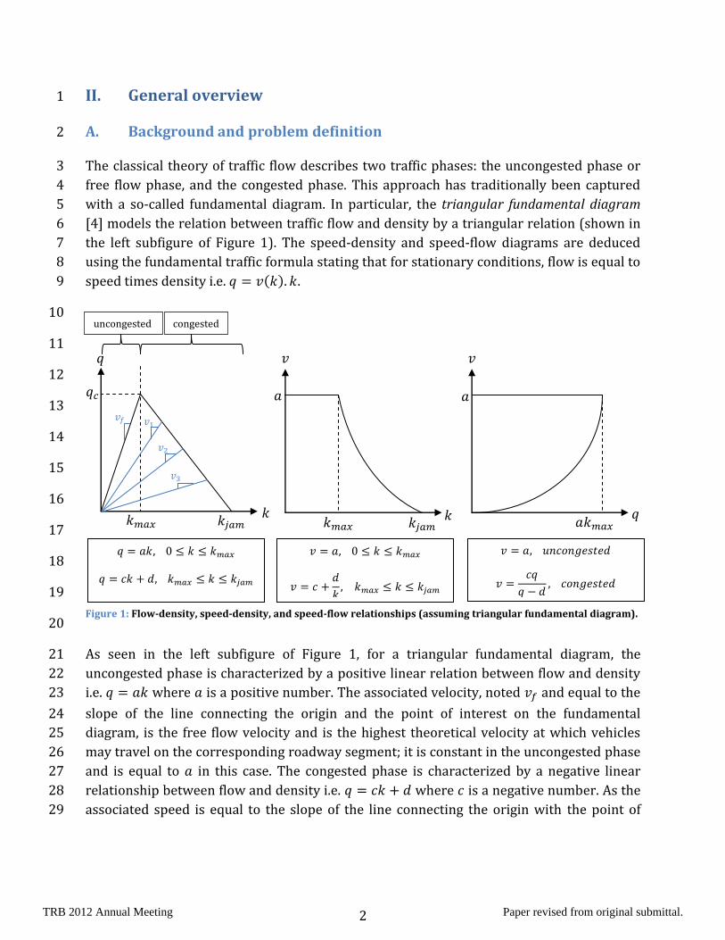
The classical theory of traffic flow describes two traffic phases: the uncongested phase or 3

free flow phase, and the congested phase. This approach has traditionally been captured 4

with a so-called fundamental diagram. In particular, the triangular fundamental diagram 5

[4] models the relation between traffic flow and density by a triangular relation (shown in 6

the left subfigure of Figure 1). The speed-density and speed-flow diagrams are deduced 7

using the fundamental traffic formula stating that for stationary conditions, flow is equal to 8

speed times density i.e. ( ) . 9

10

11

12

13

14

15

16

17

18

19

20

As seen in the left subfigure of Figure 1, for a triangular fundamental diagram, the 21

uncongested phase is characterized by a positive linear relation between flow and density 22

i.e. where is a positive number. The associated velocity, noted and equal to the 23

slope of the line connecting the origin and the point of interest on the fundamental 24

diagram, is the free flow velocity and is the highest theoretical velocity at which vehicles 25

may travel on the corresponding roadway segment; it is constant in the uncongested phase 26

and is equal to in this case. The congested phase is characterized by a negative linear 27

relationship between flow and density i.e. where is a negative number. As the 28

associated speed is equal to the slope of the line connecting the origin with the point of 29

Figure 1: Flow-density, speed-density, and speed-flow relationships (assuming triangular fundamental diagram).

congested uncongested


3

interest on the fundamental diagram, speed decreases with density in this phase; this is 1

illustrated in the middle subfigure of Figure 1. 2

In the uncongested phase, velocity remains constant at the free-flow speed. This models the 3

fact that up to a certain threshold density, the spacing between vehicles travelling on a 4

roadway segment is sufficiently large for commuters not to be affected or constrained by 5

surrounding vehicles, and as such they travel at the free-flow speed. 6

As seen in the fundamental and speed-flow diagrams in Figure 1, the speed-to-flow 7

conversion is straightforward in the congested phase as speed monotonically decreases 8

with density in said state. In the uncongested phase, however, the conversion is 9

theoretically impossible as speed is theoretically constant at the free-flow speed. The 10

reader is referred to [5] and [6] for related research on the topic. 11

B. Learning improved speed/flow relation 12

A natural method of conversion consists in using a classical regression in speed-flow 13

coordinates. Joint measurements of speed and flow are gathered in a learning phase, and a 14

linear regression is run on the data corresponding to the uncongested state. As is 15

empirically shown in a subsequent section of this report, this method yields results that are 16

not always accurate and provides only a “blurred” picture of ground truth flow. A 17

competing technique is thus desirable. 18

This article proposes and investigates the performance of an alternative conversion 19

technique based on individual speed variances. The intuition behind it is the following: in 20

the uncongested phase, at low flows, commuters are able to drive at the speed they 21

feel comfortable with; hence individual speed variance is expected to be relatively 22

large. At higher flows, however, in the uncongested phase, the individual speed 23

variance is expected to be relatively small because commuters are constrained by 24

other surrounding vehicles and hence cannot freely choose their traveling speeds. 25

This hypothesis therefore postulates a decreasing relationship between individual speed 26

variance and flow in the uncongested phase. 27

III. Data and methodology 28

A. Data source and format 29

The dataset used in this analysis consists of speeds and flows of vehicles travelling on 30

highway and freeway segments, as recorded by 112 radars in the Bay Area, California, 31

during the month of September 2010. The radars output speed (miles per hour) and flow 32

(vehicles per minute) measurements per lane of roadway for every minute of every hour of 33


4

every day. The raw data was derived from NAVTEQ Traffic Patterns™ and made available to 1

the California Center for Innovative Transportation courtesy of the NAVTEQ University 2

Program (http://www.NN4D.com/university). Traffic Patterns data © 2011 NAVTEQ. 3

B. Methodology 4

The validity of the proposed speed-to-flow conversion method is assessed by computation 5

of different statistics for each of the 112 available radars. The following sections discuss the 6

experimental procedures considered. 7

1. Aggregate speed/flow diagrams 8

The aggregate speed/flow diagrams are relations between speed and flow at the radar 9

location. Total flow in every minute is simply the sum of the flows on each lane during that 10

minute. In other words, total flow is the number of cars traveling on the highway facility 11

that pass the radar location every minute. Speed is the flow-weighted speed i.e. the average 12

speed over all lanes weighted by the flow prevailing on each of these lanes. It reads: 13

∑

∑

14

where: is the flow-weighted speed in the minute of interest 15 l is the number of lanes 16

is the average speed of vehicles on lane i in the minute of interest 17 is the flow on lane i in the minute of interest 18 19

The interested reader is referred to [7] for more information concerning flow-weighted 20

speed quantities. If all flows are equal to zero, the flow-weighted speed is not defined as 21

there is no car passing by and hence there is no speed for which we can compute an 22

‘average’. Note however that this is a very rare case. 23

2. Variance computation 24

In the process of evaluating the relationship postulated to exist between speed variance 25

and flow, four different speed variances are computed. These are defined below and 26

described in greater detail in the subsequent sections: 27

Variance over time of Flow-Weighted Speeds: This variance is noted as ( ) 28

where the subscript ‘t’ stands for time and the superscript ‘as’ stands for aggregated 29

speeds. 30

Variance over time of Individual-Lane Speeds: This variance is noted as ( ) 31

where the subscript ‘t’ stands for time as before and the superscript ‘is’ stands for 32

individual speeds. 33


5

Variance over flow of Flow-Weighted Speeds (speeds higher than critical speed): 1

This variance is noted as ( ) where the subscript ‘f’ stands for flow and the 2

superscript ‘as’ stands for aggregated speed. 3

Variance over flow of Individual-Lane Speeds (speeds higher than critical speed): 4

This variance is noted as ( ). 5

The computation of the variance over flow is required for evaluating the relationship 6

between speed variance and flow and assessing the existence of a decreasing relation 7

between the two quantities. 8

The variance over time is computed for estimating the flow from the speed variance under 9

the assumption of local traffic stationarity. Indeed, in a practical setting where no loop 10

detector is available, the speed variance for a given flow cannot be computed since no flow 11

measurement is available. Hence the speed variance over time, which is the only quantity 12

which can be computed from streaming point speed, is used equivalently under the 13

assumption of local stationarity. 14

a) Variance over time 15

(1) Aggregate speeds 16

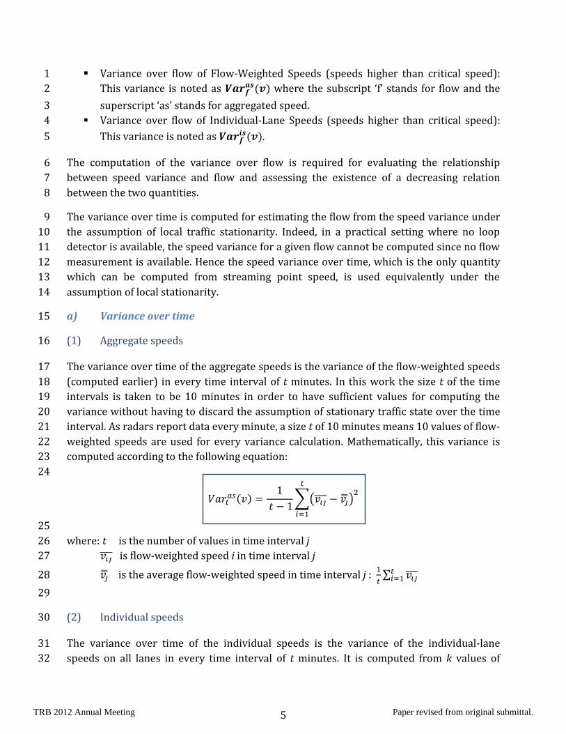
The variance over time of the aggregate speeds is the variance of the flow-weighted speeds 17

(computed earlier) in every time interval of t minutes. In this work the size t of the time 18

intervals is taken to be 10 minutes in order to have sufficient values for computing the 19

variance without having to discard the assumption of stationary traffic state over the time 20

interval. As radars report data every minute, a size t of 10 minutes means 10 values of flow-21

weighted speeds are used for every variance calculation. Mathematically, this variance is 22

computed according to the following equation: 23

24

( )

∑( )

25

where: t is the number of values in time interval j 26

is flow-weighted speed i in time interval j 27

is the average flow-weighted speed in time interval j :

∑ 28

29

(2) Individual speeds 30

The variance over time of the individual speeds is the variance of the individual-lane 31

speeds on all lanes in every time interval of t minutes. It is computed from k values of 32


6

individual speeds where k is equal to t times the number of lanes on the highway/freeway 1

facility. Mathematically, it is calculated according to the following equation: 2

( )

∑ ( )

3

4

where: l is the number of lanes of the roadway segment at the radar location of interest 5

t is the time interval size in minutes 6

is the average vehicle individual-lane speed in the minute of interest in time 7

interval j 8

is the average vehicle individual-lane speed over time interval j:

∑ 9

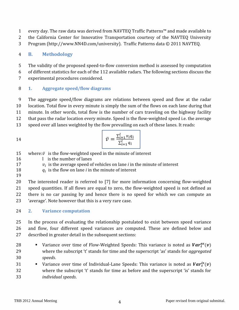
b) Variance over flow 10

(1) Aggregate speeds 11

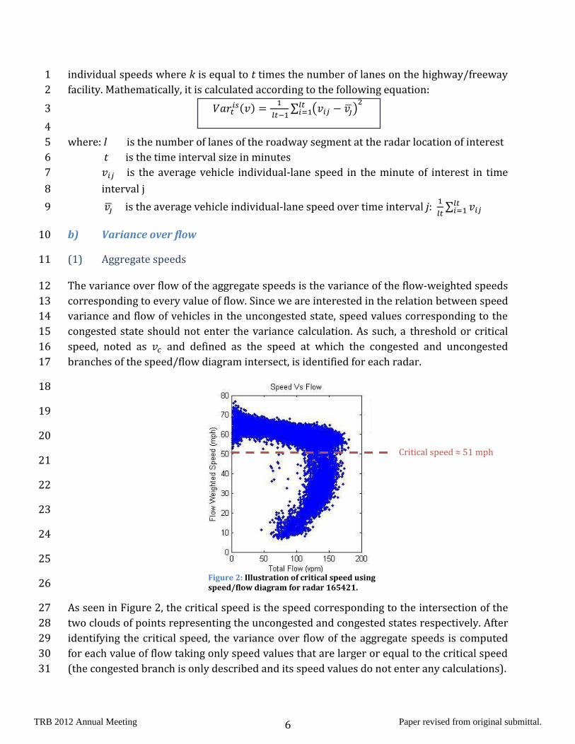
The variance over flow of the aggregate speeds is the variance of the flow-weighted speeds 12

corresponding to every value of flow. Since we are interested in the relation between speed 13

variance and flow of vehicles in the uncongested state, speed values corresponding to the 14

congested state should not enter the variance calculation. As such, a threshold or critical 15

speed, noted as and defined as the speed at which the congested and uncongested 16

branches of the speed/flow diagram intersect, is identified for each radar. 17

18

19

20

21

22

23

24

25

26

As seen in Figure 2, the critical speed is the speed corresponding to the intersection of the 27

two clouds of points representing the uncongested and congested states respectively. After 28

identifying the critical speed, the variance over flow of the aggregate speeds is computed 29

for each value of flow taking only speed values that are larger or equal to the critical speed 30

(the congested branch is only described and its speed values do not enter any calculations). 31

Critical speed ≈ 51 mph

Figure 2: Illustration of critical speed using speed/flow diagram for radar 165421.


7

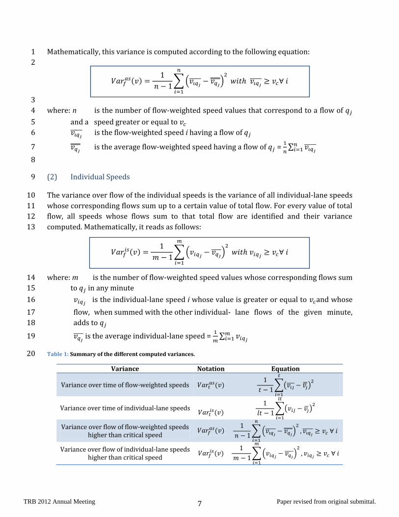
Mathematically, this variance is computed according to the following equation: 1

2

( )

∑( )

3

where: n is the number of flow-weighted speed values that correspond to a flow of 4

and a speed greater or equal to 5

is the flow-weighted speed i having a flow of 6

is the average flow-weighted speed having a flow of =

∑ 7

8

(2) Individual Speeds 9

The variance over flow of the individual speeds is the variance of all individual-lane speeds 10

whose corresponding flows sum up to a certain value of total flow. For every value of total 11

flow, all speeds whose flows sum to that total flow are identified and their variance 12

computed. Mathematically, it reads as follows: 13

( )

∑( )

where: m is the number of flow-weighted speed values whose corresponding flows sum 14

to in any minute 15

is the individual-lane speed i whose value is greater or equal to and whose 16

flow, when summed with the other individual- lane flows of the given minute, 17

adds to 18

is the average individual-lane speed =

∑ 19

Table 1: Summary of the different computed variances. 20

Variance Notation Equation

Variance over time of flow-weighted speeds ( )

∑( )

Variance over time of individual-lane speeds

( )

∑( )

Variance over flow of flow-weighted speeds higher than critical speed

( )

∑( )

Variance over flow of individual-lane speeds higher than critical speed

( )

∑( )


8

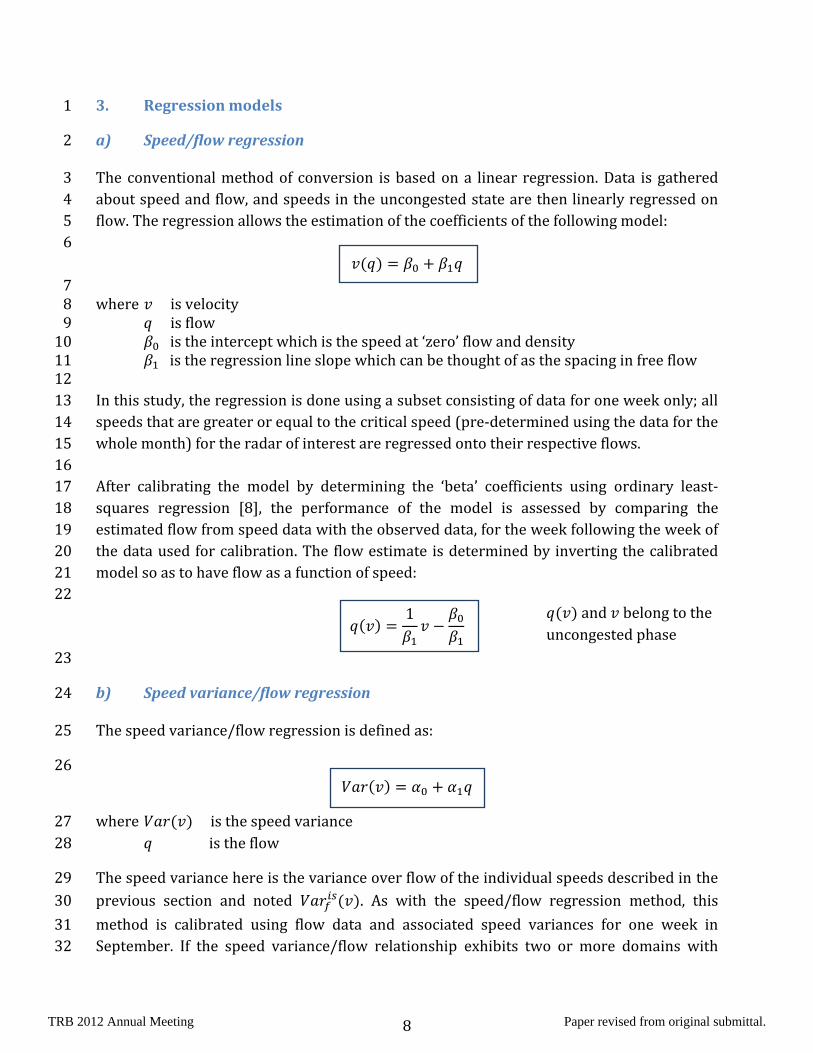
3. Regression models 1

a) Speed/flow regression 2

The conventional method of conversion is based on a linear regression. Data is gathered 3

about speed and flow, and speeds in the uncongested state are then linearly regressed on 4

flow. The regression allows the estimation of the coefficients of the following model: 5

6

( )

7 where is velocity 8 is flow 9 is the intercept which is the speed at ‘zero’ flow and density 10 is the regression line slope which can be thought of as the spacing in free flow 11 12

In this study, the regression is done using a subset consisting of data for one week only; all 13

speeds that are greater or equal to the critical speed (pre-determined using the data for the 14

whole month) for the radar of interest are regressed onto their respective flows. 15

16

After calibrating the model by determining the ‘beta’ coefficients using ordinary least-17

squares regression [8], the performance of the model is assessed by comparing the 18

estimated flow from speed data with the observed data, for the week following the week of 19

the data used for calibration. The flow estimate is determined by inverting the calibrated 20

model so as to have flow as a function of speed: 21

22

( )

23

b) Speed variance/flow regression 24

The speed variance/flow regression is defined as: 25

26

( )

where ( ) is the speed variance 27

is the flow 28

The speed variance here is the variance over flow of the individual speeds described in the 29

previous section and noted ( ). As with the speed/flow regression method, this 30

method is calibrated using flow data and associated speed variances for one week in 31

September. If the speed variance/flow relationship exhibits two or more domains with 32

( ) and belong to the

uncongested phase


9

significantly different slopes, a separate regression is done on each domain separately, in 1

order to have a piecewise linear relationship such as the one shown in Figure 3. 2

3

4

5

6

7

8

9

10

11

12

13

14

15

16

17

18

19

Similarly, the model performance is assessed by inverting the previous equation and 20

comparing the flow estimate with the observed flow using data corresponding to the week 21

that follows the week used for calibration. The inverted equation is: 22

23

24

( ( ))

( )

25

26

It is to be reminded that the speed variance in the model is ( ) as described earlier. A 27

priori knowledge of flow is not known however and therefore it is not possible to identify 28

all individual speed values that have flows that sum up to a certain total flow value in order 29

to compute their variance. Hence, an assumption of locally stationary traffic is required. 30

Total flow is consequently assumed to be constant over each time interval and speed 31

variance is computed by computing the variance of all individual-lane speeds in each time 32

interval, excluding those speeds under the predetermined critical speed for the radar of 33

interest. The flow is then determined from the calibrated model and is compared with the 34

observed flow prevailing in the corresponding time interval. 35

Figure 3: Example of piecewise linear regression of speed variance over flow.


10

IV. Results 1

A. Aggregate speed/flow diagrams 2

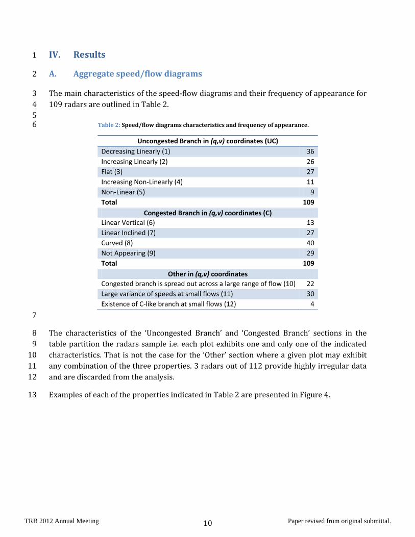
The main characteristics of the speed-flow diagrams and their frequency of appearance for 3

109 radars are outlined in Table 2. 4

5 Table 2: Speed/flow diagrams characteristics and frequency of appearance. 6

Uncongested Branch in (q,v) coordinates (UC)

Decreasing Linearly (1) 36

Increasing Linearly (2) 26

Flat (3) 27

Increasing Non-Linearly (4) 11

Non-Linear (5) 9

Total 109

Congested Branch in (q,v) coordinates (C)

Linear Vertical (6) 13

Linear Inclined (7) 27

Curved (8) 40

Not Appearing (9) 29

Total 109

Other in (q,v) coordinates

Congested branch is spread out across a large range of flow (10) 22

Large variance of speeds at small flows (11) 30

Existence of C-like branch at small flows (12) 4

7

The characteristics of the ‘Uncongested Branch’ and ‘Congested Branch’ sections in the 8

table partition the radars sample i.e. each plot exhibits one and only one of the indicated 9

characteristics. That is not the case for the ‘Other’ section where a given plot may exhibit 10

any combination of the three properties. 3 radars out of 112 provide highly irregular data 11

and are discarded from the analysis. 12

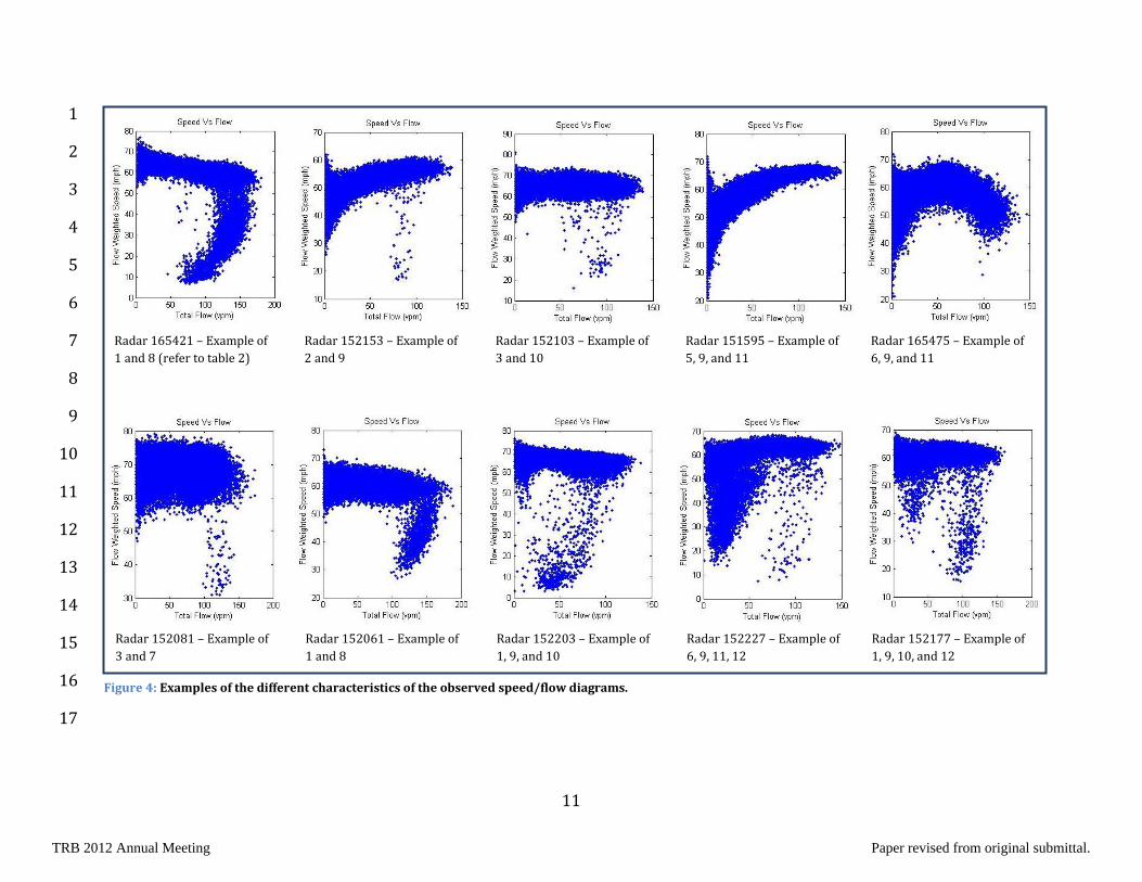
Examples of each of the properties indicated in Table 2 are presented in Figure 4.13


11

1

2

3

4

5

6

7

8

9

10

11

12

13

14

15

16

17

Radar 165421 – Example of

1 and 8 (refer to table 2)


2 and 9


3 and 10


5, 9, and 11


6, 9, and 11


3 and 7


1 and 8


1, 9, and 10


6, 9, 11, 12


1, 9, 10, and 12

Figure 4: Examples of the different characteristics of the observed speed/flow diagrams.


12

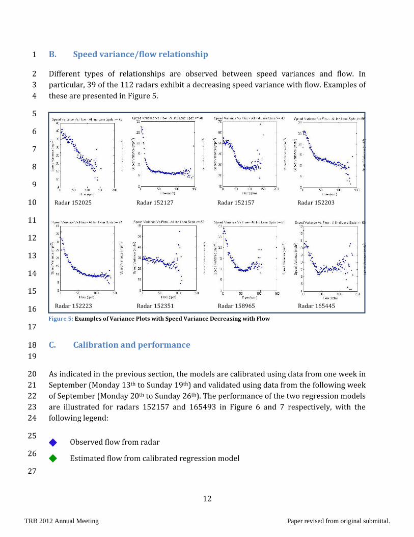
B. Speed variance/flow relationship 1

Different types of relationships are observed between speed variances and flow. In 2

particular, 39 of the 112 radars exhibit a decreasing speed variance with flow. Examples of 3

these are presented in Figure 5. 4

5

6

7

8

9

10

11

12

13

14

15

16

17

C. Calibration and performance 18

19

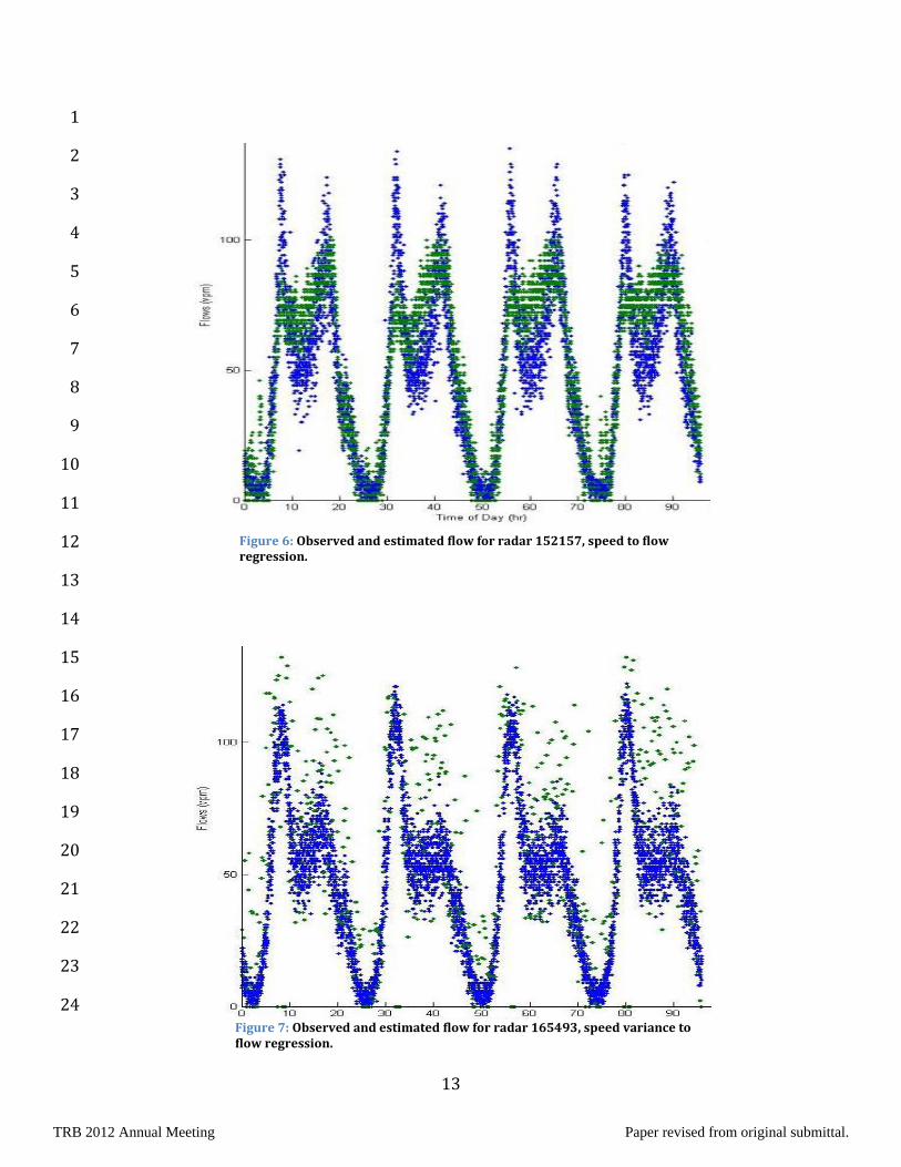
As indicated in the previous section, the models are calibrated using data from one week in 20

September (Monday 13th to Sunday 19th) and validated using data from the following week 21

of September (Monday 20th to Sunday 26th). The performance of the two regression models 22

are illustrated for radars 152157 and 165493 in Figure 6 and 7 respectively, with the 23

following legend: 24

25

26

27

Radar 152223 Radar 152351 Radar 158965 Radar 165445

Radar 152025 Radar 152127 Radar 152157 Radar 152203

Figure 5: Examples of Variance Plots with Speed Variance Decreasing with Flow

Observed flow from radar

Estimated flow from calibrated regression model


13

1

2

3

4

5

6

7

8

9

10

11

12

13

14

15

16

17

18

19

20

21

22

23

24

Figure 6: Observed and estimated flow for radar 152157, speed to flow regression.

Figure 7: Observed and estimated flow for radar 165493, speed variance to flow regression.


14

20 17

20

7 10

7

0

5

10

15

20

25

30

Increasing UCBranch

Large Variance ofSpeeds at low

flows

C not appearingor marked by

few points

Other

DominantCharacteristic

10

9

11 Increasing UC

Decreasing UC

Flat UC

V. Discussion and analysis 1

A. Speed variance/flow taxonomy 2

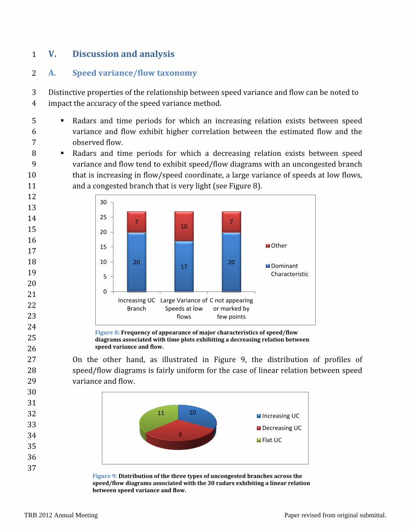
Distinctive properties of the relationship between speed variance and flow can be noted to 3

impact the accuracy of the speed variance method. 4

Radars and time periods for which an increasing relation exists between speed 5

variance and flow exhibit higher correlation between the estimated flow and the 6

observed flow. 7

Radars and time periods for which a decreasing relation exists between speed 8

variance and flow tend to exhibit speed/flow diagrams with an uncongested branch 9

that is increasing in flow/speed coordinate, a large variance of speeds at low flows, 10

and a congested branch that is very light (see Figure 8). 11

12

13

14

15

16

17

18

19

20

21

22

23

24

25

26

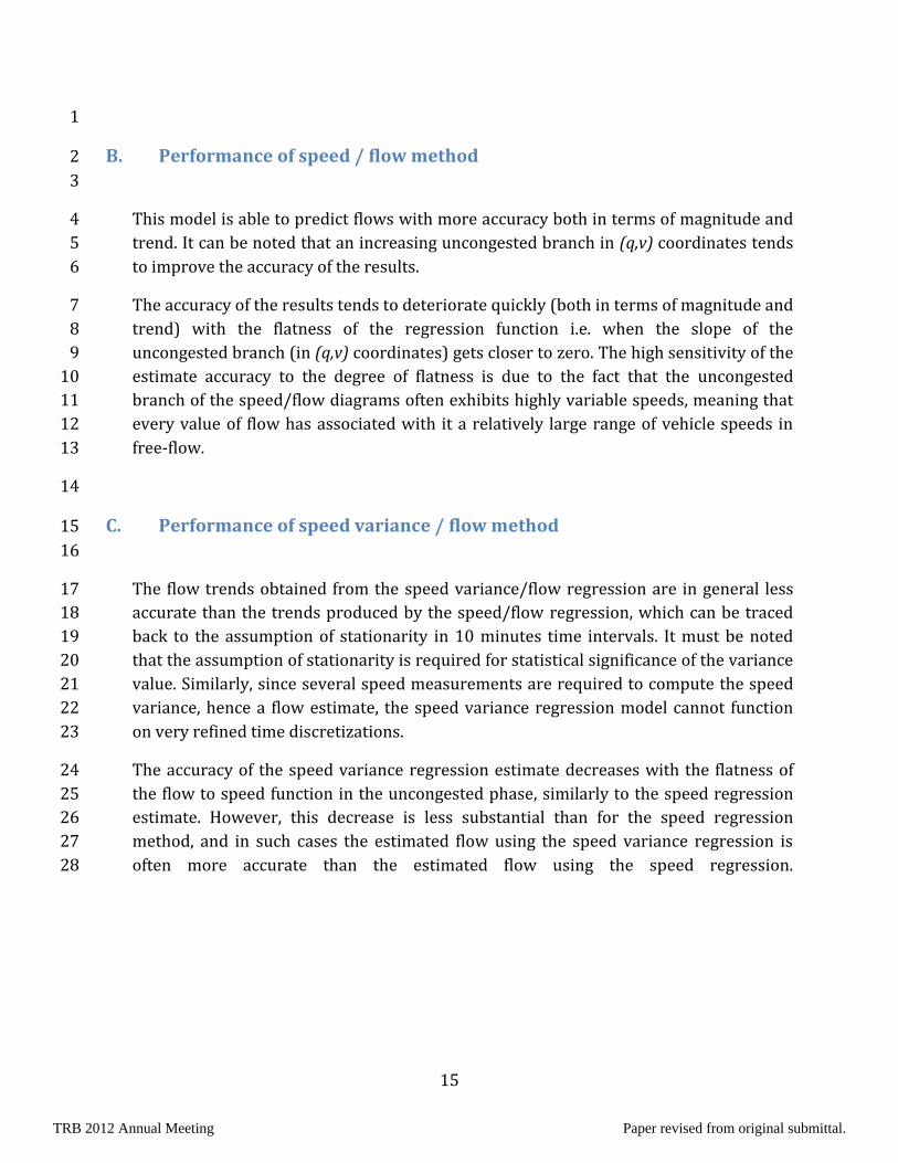
On the other hand, as illustrated in Figure 9, the distribution of profiles of 27

speed/flow diagrams is fairly uniform for the case of linear relation between speed 28

variance and flow. 29

30

31

32

33

34

35

36

37

Figure 8: Frequency of appearance of major characteristics of speed/flow diagrams associated with time plots exhibiting a decreasing relation between speed variance and flow.

Figure 9: Distribution of the three types of uncongested branches across the speed/flow diagrams associated with the 30 radars exhibiting a linear relation between speed variance and flow.


15

1

B. Performance of speed / flow method 2

3

This model is able to predict flows with more accuracy both in terms of magnitude and 4

trend. It can be noted that an increasing uncongested branch in (q,v) coordinates tends 5

to improve the accuracy of the results. 6

The accuracy of the results tends to deteriorate quickly (both in terms of magnitude and 7

trend) with the flatness of the regression function i.e. when the slope of the 8

uncongested branch (in (q,v) coordinates) gets closer to zero. The high sensitivity of the 9

estimate accuracy to the degree of flatness is due to the fact that the uncongested 10

branch of the speed/flow diagrams often exhibits highly variable speeds, meaning that 11

every value of flow has associated with it a relatively large range of vehicle speeds in 12

free-flow. 13

14

C. Performance of speed variance / flow method 15

16

The flow trends obtained from the speed variance/flow regression are in general less 17

accurate than the trends produced by the speed/flow regression, which can be traced 18

back to the assumption of stationarity in 10 minutes time intervals. It must be noted 19

that the assumption of stationarity is required for statistical significance of the variance 20

value. Similarly, since several speed measurements are required to compute the speed 21

variance, hence a flow estimate, the speed variance regression model cannot function 22

on very refined time discretizations. 23

The accuracy of the speed variance regression estimate decreases with the flatness of 24

the flow to speed function in the uncongested phase, similarly to the speed regression 25

estimate. However, this decrease is less substantial than for the speed regression 26

method, and in such cases the estimated flow using the speed variance regression is 27

often more accurate than the estimated flow using the speed regression.28


16

VI. Conclusions 1

This article proposed the analysis of the relation between point speed and flow. 2

Performance assessment of different techniques for accurate conversion of point speeds to 3

point flows was conducted, in the prospect of fusing speed data with conventional loop 4

detectors. 5

The study used speed and flow measurements from September 2010, obtained from 112 6

NAVTEQ radars [1] deployed in the San Francisco Bay Area. The major steps of the analysis 7

presented are the following: 8

Evaluation and categorization of 112 measured speed/flow diagrams, 9

Evaluation of 112 measured variance plots, 10

Comparative benchmark of the speed variance to flow regression method with the 11

speed to flow regression method. 12

The main conclusions of this study are the following. 13

The conventional speed/flow method is able to produce significantly more accurate results 14

than the speed variance/flow method, in particular in the case of an increasing 15

uncongested branch in (q,v) coordinates, which is not predicted by the theory. This 16

accuracy deteriorates quickly however when the uncongested branch of the diagram in 17

(q,v) coordinated becomes more flat. 18

The proposed speed variance/flow method does not achieve the accuracy obtained with 19

the conventional method; this may be due to the assumption of stationarity, required for 20

statistically significant computation of the speed variance. The proposed method, however, 21

shows more accurate results than the traditional method in the case where the 22

uncongested branch in (q,v) coordinates is relatively flat, which is a classical assumption on 23

the free-flow phase. 24

The preliminary assessment proposed in this work shows promising results, with two 25

methods with complementary behaviors providing reasonably accurate flow estimates. In 26

particular, the evidence for traffic behaviors not well modeled by traffic theory and the 27

characterization of the specific traffic episodes for which each method performs better lays 28

the ground for more refined analytics. Further efforts on the topic encompass the use of a 29

rigorous estimation setting for quantitative assessment of the proposed methods for 30

specific applications. 31

32

33


17

Acknowledgments 1

2

We want to acknowledge NAVTEQ for their ongoing support and for the partnership with 3

UC Berkeley. In particular we are grateful to Candace Sleeman for her help with University 4

Relations, Brian Smith and Drew Bittenbender for their help with setting up data exchange 5

feeds with NAVTEQ. We want to thank the California Center for Innovative Transportation 6

(CCIT) team for their help with this project, in particular Joe Butler, Ali Mortazavi, Saneesh 7

Apte and Jonathan Felder. Finally, we want to thank the California DOT for their ongoing 8

support to UC Berkeley and their interest in data fusion and hybrid data. Particular thanks 9

go to John Wolf, Joan Sollenberger and Nicholas Compin for their guidance. 10

References 11

12

[1] NAVTEQ Traffic Patterns™, North America. Traffic Patterns data provided courtesy 13

of the NAVTEQ University Program (http://www.NN4D.com/university), © 2011 14

NAVTEQ. 15

[2] B. COIFMAN, Improved velocity estimation using single loop detectors, 16

Transportation Research Part A: Policy and Practice 35 (10), pp.863—880, (2001). 17

[3] H. RAKHA and W. ZHANG, Estimating traffic stream space-mean speed and 18

reliability from dual and single loop detectors, Transportation Research Record 19

1925, pp.38—47, (2005). 20

[4] C.F. DAGANZO, The cell-transmission model, part II: network traffic, Transportation 21

Research Part B: Methodological, 29(2), pp.79--93 (1995). 22

[5] O.A. NIELSEN and R.M. JORGENSEN, Estimation of speed--flow and flow—density 23 relations on the motorway network in the greater Copenhagen region, IET Intell. 24 Transp. Syst. 2(2),pp. 120-131 (2008). 25

26 [6] M. J. CASSIDY and B. COIFMAN, Relation among average speed, flow, and density and 27

analogous relation between density and occupancy, Transportation Research 28

Record 1591, pp. 1—6 (1997). 29

[7] C.F. DAGANZO, Fundamentals of transportation and traffic operations, Pergamon, 30

Oxford, (1997). 31

[8] C.R. RAO, Linear statistical inference and its applications, Wiley, New-York, (2002). 32


individual speed variance in traffic flow: analysis of … speed variance in traffic flow: analysis...

Documents