Individual and Aggregate Labor Supply With

Coordinated Working Times

Richard Rogerson

Arizona State University

October 2009

Preliminary and Incomplete Please Do Not Quote

Abstract

I analyze two extensions to the standard model of life cycle labor supplythat feature operative choices along both the intensive and extensive mar-gin. The first assumes that individuals face different continuous wage-hoursschedules. The second assumes that all work must be coordinated acrossindividuals. These models look similar qualitatively but have very differentimplications for how aggregate labor supply responds to changes in taxes.In the first model, curvature in the utility from leisure function plays rela-tively little role in determining the overall change in hours worked, whereasin the second model it is of first order importance. The second model hasimportant implications for what data is most able to provide evidence onthe extent of curvature in the utility from leisure function.

1. Background and Introduction

Starting with the contribution of Lucas and Rapping (1969) and continuing with

the development of modern business cycle theory by Kydland and Prescott (1982),

economists have sought to understand aggregate labor market outcomes using a

framework in which individual economic agents solve explicit optimization prob-

lems and interact through explicitly specified market structures and/or other chan-

nels. One critique of early work in this research program concerned the relation-

ship between individual and aggregate labor supply elasticities. Specifically, in

the early representative agent models that dominated the literature and featured

solely an intensive margin of labor supply, an exercise of the sort pioneered by

MaCurdy(1981) would uncover the value of the key preference parameter that per-

fectly characterized both individual and aggregate labor supply responses. This

raised an immediate problem, since the implied elasticities from micro data were

much smaller than the implied elasticities from aggregate data. While some con-

cluded that this inconsistency was evidence against the overall approach empha-

sized by this research program, in his discussion of Kydland (1984), Heckman

(1984) offered a different assessment. He suggested that the key underlying issue

was that the models being used both in micro and aggregate studies were abstract-

ing from key features of individual labor supply problems, limiting the usefulness

of comparisons across these studies. Specifically, he argued that because adjust-

ment at the extensive margin is so prevalent at the individual level, any compelling

analysis that seeks to derive aggregate implications from individual choice prob-

1

lems would have to incorporate an extensive margin into the analysis.1 Given

such a model, it was not clear what the implications would be for aggregate labor

supply, nor what the significance of the MaCurdy style estimates for prime aged

males would be, since these estimates seemed only to reveal information about

intensive margin adjustments for one groups of workers.

One interpretation of the comments in Heckman (1984) is that they issued

a call to develop models which simultaneously capture the important margins of

individual labor supply, allow for a rich structure of heterogeneity, and permit

us to solve for aggregate outcomes. This would allow us to connect analysis of

both individual and aggregate data in a consistent framework. A simple reality

of economic analysis is that the quantitative implications of any particular model

typically depend on the various features and parameter values that characterize

the individual decision problems. Some features that are “realistic” may turn out

to not be quantitatively important in terms of substantive economic implications.

One of the key objective of economic research is to sort out the important from

the not-so-important features in the context of specific issues that we want to

address. To carry out this type of analysis in a consistent fashion requires exactly

the sort of model just described.

Shortly after Heckman’s (1984) comments, macroeconomists found a way to

tractably introduce an extensive margin of labor supply into their models. Hansen

(1985) introduced the indivisible labor assumption of Rogerson (1988) into an oth-

erwise standard aggregate model. While in principle this could have facilitated

1Heckman (1993) also emphasized the importance of heterogeneity and the extensive marginin connecting individual labor supply with aggregate labor supply.

2

a greater connection between these models and the micro data on labor supply,

in fact it had somewhat of the opposite effect, the immediate effect was almost

the opposite. A key property of these representative household models was that

the aggregate labor supply elasticity was large independently of the value of the

elasticity parameter estimated by MaCurdy and others. As a result, many macro-

economists viewed the indivisible labor assumption as a justification to not look at

the micro data on labor supply, since one prominent component of the literature

was focused on a parameter which was no longer relevant. Browning et al (1998)

pointed out this disconnect from the micro data. In particular, while the equi-

librium allocation that Hansen (1985) and others emphasized were an important

improvement over the earlier models because of the presence of adjustment along

the extensive margin, the individual employment histories in these models did not

correspond at all to those found in the data.2

The last ten years has witnessed some important extensions of the basic indi-

visible labor model, and puts us in a position to be able to address micro level

observations and aggregate implications within a consistent model. Of particular

interest is the work by Chang and Kim (2006, 2007, 2009). These authors study

models that feature idiosyncratic shocks, incomplete markets and indivisible la-

bor choice.3 In the context of this model, one can carry out the same types of

2Browning et al (1998) claimed that the Hansen (1985) model implied equal employmentprobabilities next period for both the current employed and non-employed. In fact, the structureof the transitions is actually indeterminate. While this implies that the data are not inconsistentwith the model, the model certainly does not help us understand why we see particular patternsin terms of movements between employment and non-employment.

3These models follow the important earlier contributions of Huggett (1993), Aiyagari (1994)and Krusell and Smith (1998).

3

individual level estimation exercises that MaCurdy (1981) and others performed,

at the same time that one can examine the implications of aggregate shocks for

aggregate hours of work in the spirit of Kydland and Prescott (1982).4 In the

context of these models, the old micro data estimates do not turn out to be of

great importance, at the same time that aggregate labor supply is somewhat less

elastic than in the earlier representative agent models. More recently, Krusell et

al (2009a, b) add trading frictions to this framework and show that it can also ac-

count for the flows of individual workers between the employment, unemployment

and out of the labor force states. French (2004) and Low et al (2009) show in

partial equilibrium settings that a model of this sort is also consistent with many

features of life cycle labor supply.

In summary, much has changed over the last 25 or so years. Viewed from the

perspective of the current models that economists are using, the initial controversy

about individual and aggregate labor supply elasticities based on importing the

estimates of MaCurdy into aggregate representative agent models seems some-

what archaic. We can now explore which features are important in accounting

for various aspects of micro level data and assess the importance of these features

for various issues that involve aggregate outcomes. While we now have a solid

foundation, there are still many open issues, dealing with such issues as the im-

portance of various types of shocks, the nature of human capital accumulation,

4Chang and Kim (2009) also revisits the contribution of Mankiw et al (1986) and showsthat if one tries to interpret the aggregate data in this model as coming from a representativehousehold that only adjusts labor along the intensive margin, that one obtains the same typesof problematic results that these authors find, i.e., parameter estimates of the wrong sign andviolation of concavity.

4

the importance of different sources of heterogeneity, the role of market structure,

trading frictions, family structure etc....

Choice along the extensive margin figures prominently in the class of models

just described. In these models the extensive margin is introduced by assumption—

in any given period the individual is assumed to have only two choices—work some

pre-specified number of hours, or work zero hours. At a descriptive level, this

assumption seems empirically reasonable, corresponding to the observation that

there is a great deal of concentration in the distribution of work hours, either at

the weekly or even annual level. But while the assumption of indivisible labor

is empirically descriptive, given its prominence in these models one might well

ask what deeper forces lead to this concentration of working hours, and whether

the aggregate properties of the model depend on the underlying cause of this

concentration. In this paper I take a first look at this issue. In particular, I

consider two different extensions of a standard life cycle labor supply model that

involve explicit choice along the intensive and extensive margins, each of which

represents ideas that have been explored quite a bit in the labor supply literature.

In the canonical labor supply model, an individual can work any number of hours,

and the wage per unit of time is fixed, leading to a linear budget equation. Many

researchers have commented that many factors are likely to influence the nature

of the constraint set that individuals face when making labor supply decisions,

and the two models that I consider reflect some of these comments.

The first model that I consider assumes that workers face a (continuous) menu

of hours and wage options, with the property that the wage per unit of time is

5

increasing in the volume of work performed.5 My analysis of this model largely

summarizes recent work by Prescott et al (2009) and Rogerson and Wallenius

(2007, 2009). A key feature of this first model is that workers are still free to

choose their hours of work in any given period, although the shape of the budget

set is now altered.

The second model assumes that the work schedule (i.e., intensive margin) is

a collective choice in the economy, and that once the work schedule is chosen,

the only choice that an individual worker faces is whether to work at the going

wage rate. This assumption is meant to capture the desire for coordination. The

motives for coordination may come from the need for workers within and across

firms to work together, or for individuals to coordinate leisure time and/or family

schedules. I do not model the underlying reason for coordination, and in a well

defined sense focus only the best outcome given the need to coordinate. A key

feature of this model is that given a particular collective choice for the work

schedule, a worker is not free to work any number of hours, and so it is typically

the case that the hours of work for an individual is not consistent with the hours

that he or she would choose to work in that period given the wage rate. A large

literature documents that desired and actual hours of work typically diverge.6

From the perspective of the individual worker, one can think of this model as

one in which the worker faces a discontinuous menu of wage and hours choices,

5Examples of papers that have documented the hours-wage menus include Moffitt (1984),Altonji and Paxson (1988), Biddle and Zarkin (1989), Dickens and Lundberg (1993), Keane andWolpin (2001) and Aronson and French (2004). The work of Cogan (1983) on fixed costs is alsovery relevant.

6See, for example, Kahn and Lang (1991), Bell and Freeman (2001) and Sousa-Poza andHenneberg (2003).

6

with wages equal to zero for any hours choice other than the collectively decided

value. But a key point is that the location of the discontinuity is determined by

the collective choice rather than being a feature of technology.

Consistent with the data, both of these extensions to the standard life cycle

model generate life cycle profiles for hours at the individual level in which adjust-

ment at the extensive margin plays a key role. I provide analytic and graphical

characterizations of optimal lifetime labor supply along the intensive and exten-

sive margins for both models. In each case one can view the optimal choice as the

intersection of downward and upward sloping curves in intensive margin-extensive

margin space. The differing slopes of these two curves reflects the simple reality

that from one perspective the two margins are substitutes, while from another

perspective they are complements. The sense in which the two are substitutes

is that from the perspective of generating income, one can generate income from

increasing labor supply along either margin. The sense in which the two are com-

plements is that from the perspective of efficient time allocation, disutility per

unit of income earned should be equated along all margins. This implies that one

should only more years if one is also working longer hours when working. From a

qualitative perspective, these two models seem to have much in common.

I then consider how aggregate labor supply in these models responds to an

increase in the scale of a simple tax and transfer program, and in particular, I

contrast them with the outcomes that emerge in the standard life cycle model with

only an intensive margin of adjustment. The striking finding is that the twomodels

with operative extensive margins for life cycle labor supply generate dramatically

7

different aggregate outcomes. In the standard model in which the only relevant

margin is the intensive margin, the aggregate response is tightly connected to the

preference parameter that dictates curvature in the utility from leisure. Whether

the response is large or small depends critically on this parameter. Consistent

with the results of Rogerson and Wallenius (2009), the model with an hours/wage

menu generates large responses independently of the preference parameter that

dictates curvature in the utility from leisure. In sharp contrast, the results in the

work schedule model, exactly mirror those in the standard model. The important

result that follows is that the mere presence of an important role for the extensive

margin in terms of life cycle labor supply does not necessarily generate large

aggregate elasticities.

While the work schedule model has very different implications for what factors

shape the response of aggregate hours to a change in tax and transfer programs,

it also has important implications for empirical work that aims to uncover these

factors, in particular the curvature parameter in the utility from leisure function.

Specifically, this model implies that individual labor supply responds differently

to idiosyncratic variation in driving forces than it does to aggregate variation in

driving forces. If the work schedule is a collective choice, then it will be invariant

to purely idiosyncratic variation, but not to changes in aggregate or common

factors. The implication in the stark model studied in this paper is that analysis

of micro data may not be sufficient in estimating this key preference parameter.

In particular, aggregate data may have a significant role to play in determining

8

the value of this parameter.7

An outline of the paper follows. Section 2 describes the three models and

characterizes their implications for life cycle labor supply. Section 3 considers the

implications of each model for changes in the scale of a simple tax and transfer

program, both qualitatively and in some simple numerical examples. Section 4

discusses the results of the analysis and Section 5 concludes.

2. Three Models of Life Cycle Labor Supply

In this section I describe three different models of life cycle labor supply. The first

model is a standard model in which all adjustment in labor supply takes place

along the intensive margin. The other two models both feature choice along the

intensive and extensive margins. The first of these will consider the assumption,

following Prescott et al (2009), of a nonconvex mapping from time devoted to

work to labor services. As noted in the introduction, this assumption implies

that workers face a menu of wage/hours combination when making labor supply

choices. The second of these models will be the analysis that is novel to this paper,

and will consider a case in which the individual is forced to choose a fixed work

length for all dates at which labor supply is positive. This is meant to capture the

notion that due to coordination issues, all production must be carried out with a

fixed working schedule. If this work schedule were exogenously given, this would

amount to the standard indivisible labor model of Rogerson and Hansen. But

7This issue has been recognized in the literature. See for example, Ham (1982), Biddle (1988)and Khan and Lang (1991). See also the discussion in Fehr and Goette (2007) regarding thedesirability of experimental data.

9

the novel feature here is that the work schedule is chosen by the worker at the

beginning of life.

2.1. The Standard Life Cycle Model

Because the extensions that I consider next will have implications for the fraction

of lifetime that an individual spends in employment, it is convenient to formulate

the model in continuous time, so that the labor supply choice along the extensive

margin is a continuous choice variable and can therefore be characterized using

standard methods. Consider an individual with length of life normalized to one

who has preferences defined by:

Z 1

0

[u(c(a)) + v(1− h(a))]da

where c(a) is consumption at age a, h(a) is time devoted to market work at age

a, u(·) gives the utility flow from consumption and v(·) gives the utility flow fromleisure. We assume that these two function are twice continuously differentiable,

strictly increasing, strictly concave and satisfy:

limc→0

u0(c) = +∞

limh→1

v0(1− h) = +∞

I assume that utility is separable between consumption and leisure. While this

has counterfactual implications for the behavior of consumption over the life cycle

in the analysis that follows, it serves to simplify the analytic presentation of the

10

results and so is convenient for purposes of exposition. I have also chosen to

assume that the individual does not discount future utility flows. As will become

clear shortly, this serves to simplify the analytic characterization of the solution to

the individual’s maximization problem. I will focus on the case where the interest

rate is also zero, so that these two factors will be offsetting as is standard in many

macro models with infinitely lived agents.

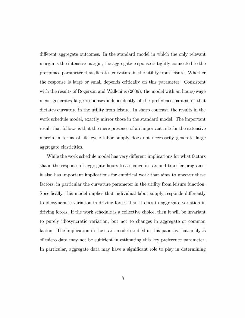
Following much of the life cycle labor supply literature, I assume that the

productivity of an individual’s time varies systematically over the life cycle. In

particular, if an individual of age a devotes h units of time to market production,

I assume that this yields e(a)h units of labor services. In the numerical work that

follows I will assume that the age profile for this productivity process follows the

shape shown in Figure 1.

A few remarks are in order regarding the assumed shape of this productivity

profile. First, for reasons of analytic tractability, I am assuming that this produc-

tivity process is exogenous, and so in particular, I am abstracting from human

capital accumulation decisions that may lie behind this profile. In the data, wages

are not symmetric over the life cycle, in the sense that wages at the end of the life

cycle are much higher than wages at the beginning of the life cycle. If one takes

wages as exogenous and assumes complete markets for borrowing and lending,

this can create a problem for a model that includes an endogenous retirement

decision. The reason for this is that there is an incentive for individuals to try to

avoid working in the early part of life in order to avoid the low wages during the

period, and to instead work more at the later part of the life cycle when wages

11

0 0.2 0.4 0.6 0.8 10.5

0.6

0.7

0.8

0.9

1

1.1

1.2

1.3

1.4

1.5

Age

Pro

duct

ivity

Figure 1: Productivity Over the Life Cycle

are higher. Wallenius (2009) develops a life cycle labor supply model with an op-

erative extensive margin and human capital accumulation, and shows how it can

match the life cycle profile for both wages and hours. To maintain tractability,

rather than include a human capital accumulation decision, I choose to abstract

from trying to match the actual profile of wages over the life cycle.

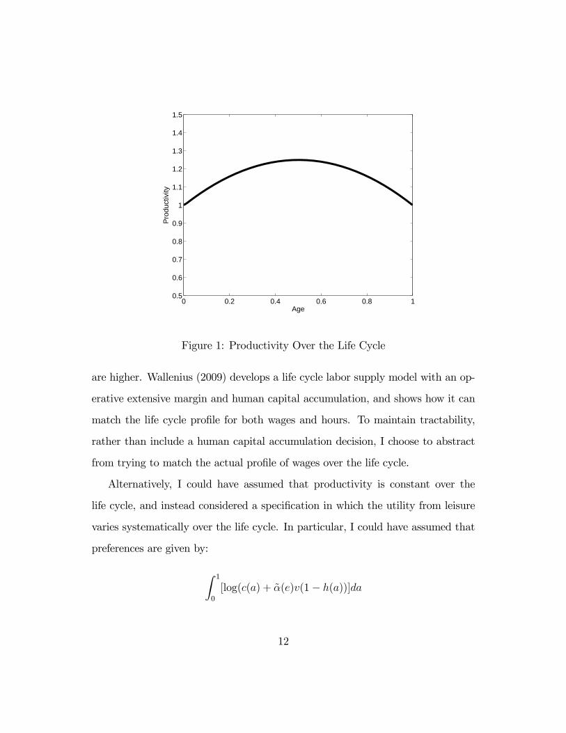
Alternatively, I could have assumed that productivity is constant over the

life cycle, and instead considered a specification in which the utility from leisure

varies systematically over the life cycle. In particular, I could have assumed that

preferences are given by:

Z 1

0

[log(c(a) + α(e)v(1− h(a))]da

12

0 0.2 0.4 0.6 0.8 10.5

0.6

0.7

0.8

0.9

1

1.1

1.2

Age

Util

ity o

f Lei

sure

Figure 2: Value of Leisure Over the Life Cycle

where α(e) has the shape given by Figure 2 below:

The key issue from a modelling perspective is to have something in the model

that gives rise to a systematic change in the static net return to working over the

life cycle. In what follows I will only consider the specification shown in Figure 1.

The wage rate per unit of labor services is assumed to be constant and equal to

w. The individual faces complete markets for borrowing and lending, so assuming

as noted above that the interest rate on borrowing and lending is equal to zero,

the present value budget equation is given by:

Z 1

0

c(a)da = w

Z 1

0

h(a)e(a)da

To this point I have only described a single agent decision problem. In the

13

subsequent analysis I will want to consider this single agent problem in the con-

text of a steady state equilibrium in an overlapping generations model. At the risk

of trivializing the general equilibrium considerations, but with the gain of trans-

parency, I will assume that we are considering a small open economy in which

the real interest rate is exogenously fixed at zero, and that there is an aggregate

production function that is linear in labor services with marginal product equal

to A.8 It follows that if the price of output is normalized to one, the equilibrium

wage rate w must be equal to A. Assuming a new generation of identical individ-

uals with total mass equal to one is born at each instant, in steady state a new

born household will solve the decision problem depicted above.

Characterizing the solution to the individual’s maximization problem is stan-

dard. The individual solves the following problem:

maxc(a),h(a)

Z 1

0

[u(c(a)) + v(1− h(a))]da

s.t.

Z 1

0

c(a)da = w

Z 1

0

h(a)e(a)da

c(a) ≥ 0, 0 ≤ h(a) ≤ 1

The solution to this problem will entail a constant flow of consumption, and hence

8The small open economy assumption is not essential. In this model one can always specifya government debt policy that will support a steady state equilibrium with a zero interest rate.

14

the problem can be rewritten as:

maxc,h(a)

u(c) +

Z 1

0

v(1− h(a))da

s.t.c = w

Z 1

0

h(a)e(a)da, 0 ≤ h(a) ≤ 1

Substituting the budget equation into the objective function, we obtain the

following condition for an interior solution for h(a):

e(a)R 10h(a)e(a)da

= v0(1− h(a)) (2.1)

which can also be written as:

v0(1− h(a)) = μwe(a) (2.2)

where μ is the marginal utility of consumption.

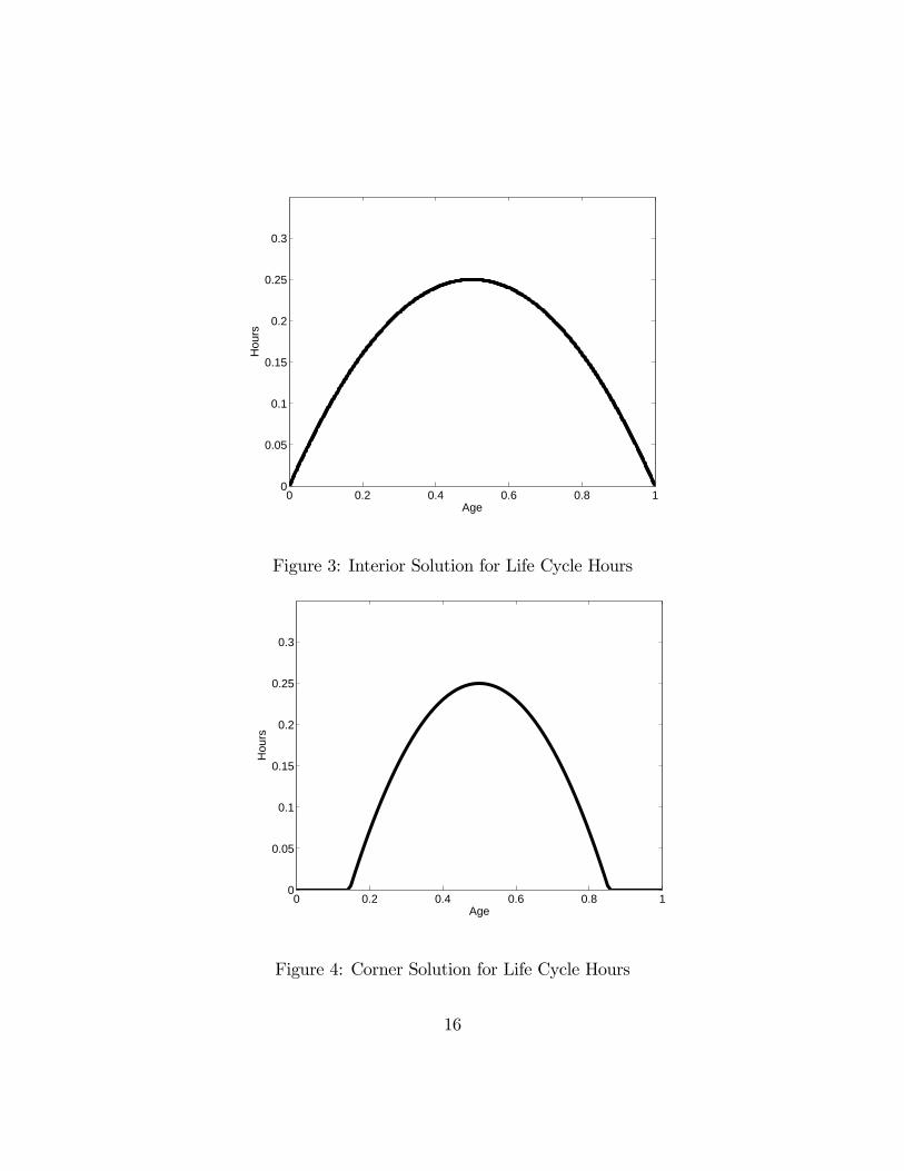
There are two different forms that the solution may take. One possibility is

that the entire profile for h(a) is positive (except possibly for the two endpoints),

as shown in Figure 3.

The other possibility is that the solution has zero hours of work for an interval

at the beginning and end of life, as shown in Figure 4.

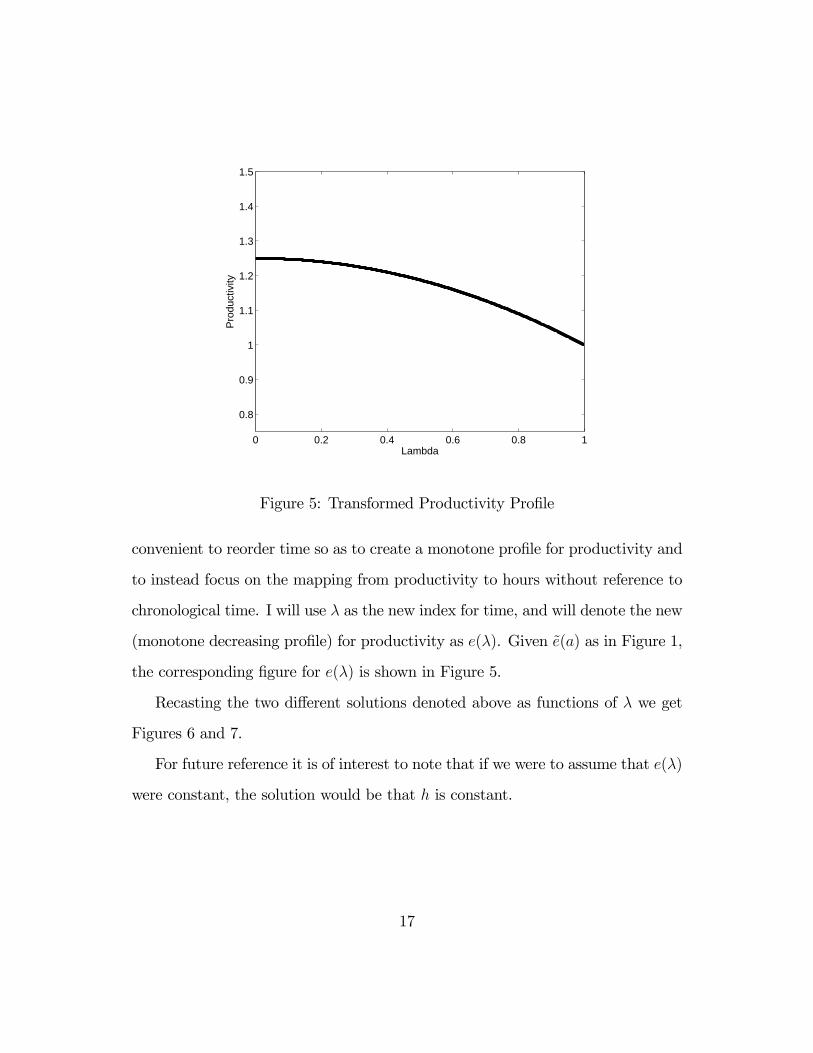
For reasons that will become clear subsequently, it is convenient to transform

the maximization problem via a simple change of variables. In particular, instead

of examining the optimal labor supply decision as a function of age, it will be

15

0 0.2 0.4 0.6 0.8 10

0.05

0.1

0.15

0.2

0.25

0.3

Age

Hou

rs

Figure 3: Interior Solution for Life Cycle Hours

0 0.2 0.4 0.6 0.8 10

0.05

0.1

0.15

0.2

0.25

0.3

Age

Hou

rs

Figure 4: Corner Solution for Life Cycle Hours

16

0 0.2 0.4 0.6 0.8 1

0.8

0.9

1

1.1

1.2

1.3

1.4

1.5

Lambda

Pro

duct

ivity

Figure 5: Transformed Productivity Profile

convenient to reorder time so as to create a monotone profile for productivity and

to instead focus on the mapping from productivity to hours without reference to

chronological time. I will use λ as the new index for time, and will denote the new

(monotone decreasing profile) for productivity as e(λ). Given e(a) as in Figure 1,

the corresponding figure for e(λ) is shown in Figure 5.

Recasting the two different solutions denoted above as functions of λ we get

Figures 6 and 7.

For future reference it is of interest to note that if we were to assume that e(λ)

were constant, the solution would be that h is constant.

17

0 0.2 0.4 0.6 0.8 10

0.05

0.1

0.15

0.2

0.25

0.3

0.35

0.4

Lambda

Hou

rs

Figure 6: Interior Hours Solution With Transformed Productivity

0 0.2 0.4 0.6 0.8 10

0.05

0.1

0.15

0.2

0.25

0.3

0.35

0.4

Lambda

Hou

rs

Figure 7: Corner Hours Solution with Transformed Productivity

18

2.2. A Nonconvex Mapping from Hours to Labor Services

Following Prescott et al (2009) and Rogerson and Wallenius (2009), this specifi-

cation modifies the worker’s problem by adding a feature to the mapping between

time devoted to work and labor services. In particular, we assume that this map-

ping features a nonconvexity. For simplicity, I focus on the special case in which

when a worker of age a devotes h units of time to market work, the resulting

supply of labor services is given by

max{h− h, 0}e(a)h

Taking into account that the worker will choose a constant profile for consumption,

the worker’s maximization problem can be written as:

maxc(,h(λ)

u(c) +

Z 1

0

v(1− h(λ))dλ

s.t.c = w

Z 1

0

max(h(λ)− h, 0)e(λ)dλ, 0 ≤ h(λ) ≤ 1

Note that the budget equation implicitly takes into account the fact that although

compensation per unit of labor services is constant and equal to w, compensation

per unit of time is non-linear in the number of hours devoted to market work. The

importance of this feature is that it creates a force for concentration of working

time as opposed to smoothing of working time. The analytics of this case are con-

tained in the somewhat more general analysis of Rogerson and Wallenius (2007),

19

0 0.2 0.4 0.6 0.8 10

0.05

0.1

0.15

0.2

0.25

0.3

0.35

0.4

Lambda

Hou

rs

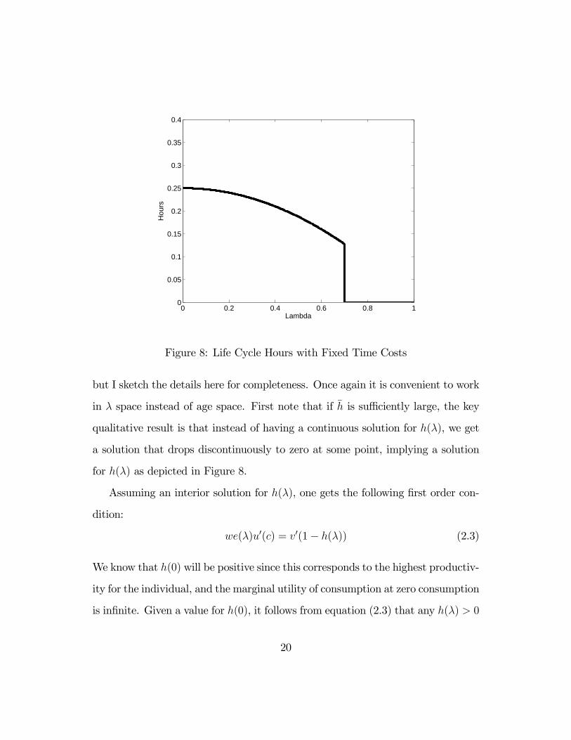
Figure 8: Life Cycle Hours with Fixed Time Costs

but I sketch the details here for completeness. Once again it is convenient to work

in λ space instead of age space. First note that if h is sufficiently large, the key

qualitative result is that instead of having a continuous solution for h(λ), we get

a solution that drops discontinuously to zero at some point, implying a solution

for h(λ) as depicted in Figure 8.

Assuming an interior solution for h(λ), one gets the following first order con-

dition:

we(λ)u0(c) = v0(1− h(λ)) (2.3)

We know that h(0) will be positive since this corresponds to the highest productiv-

ity for the individual, and the marginal utility of consumption at zero consumption

is infinite. Given a value for h(0), it follows from equation (2.3) that any h(λ) > 0

20

must satisfy:

v0(1− h(λ)) =e(λ)

e(0)v0(1− h(0)) (2.4)

Given a value for h(0) one can solve for the entire profile for h(λ) that solves equa-

tion (2.4). Since e(λ) is decreasing, it follows trivially that h(λ) is also decreasing.

If the optimal h(λ) profile were interior at all values, we would be done at this

point except for the determination of h(0). If it is not interior for all λ, the fact

that productivity is decreasing in λ, implies that a simple reservation property

holds:

h(λ) = 0 for all λ ≥ λ∗

Given a value for h(0) and the solution for h(λ) implied by equation (2.4), the

optimal value of λ /∗ is found by solving:

maxλ∗

u(c) +

Z λ∗

0

v(1− h(λ))dλ+ (1− λ∗)v(1)

s.t.c = w

Z λ∗

0

max(h(λ)− h, 0)e(λ)dλ

Assuming an interior solution, the first order condition for λ∗ is:

w(h(λ∗)− h)e(λ∗)u0(c) = v(1)− v(1− h(λ∗)) (2.5)

Combining this with equation (2.3) evaluated at λ = 0 gives:

v(1)− v(1− h(λ∗))(h(λ∗)− h)e(λ∗)

=v0(1− h(0))

e(0)(2.6)

21

Equation (2.6) represents an upward sloping relationship between h(0) and λ∗.

The economic intuition behind this relationship is that an optimal time allocation

must have the property that disutility per unit of income should be equated along

all margins. So just as equation (2.4) implies that an increase in h(0) implies an

increase in h(λ) for all λ, it is also true that an increase in h(0) implies that the

individual should work deeper into the productivity distribution.

Given h(0) and the solution for h(λ) from equation (2.4), we can represent c

as a function of h(0) and λ∗:

c = w

Z λ∗

0

max(h(λ)− h, 0)e(λ)dλ (2.7)

Since c is increasing in λ∗ it follows that equation (2.7) represents a downward

sloping relation between h(0) and λ∗. This downward sloping relation represents

the simple fact that in terms of generating consumption, the intensive and ex-

tensive choices are substitutes. That is, if an individual is working longer hours,

the value of consumption at the margin from working more along the extensive

margin is lower.

Assuming that the solution for λ∗ is interior, the intersection of these two

curves is the solution to the life cycle labor supply problem for this individual.

For future reference, I note that if the productivity profile were constant, then the

optimal solution would be that hours are constant and then drop discontinuously

to zero at some point. This highlights the sense in which this model has a force

that opposes the desire of the individual to have smooth hours of work.

22

2.3. Coordinated Working Times

In this section I add a different constraint to the standard problem. In particular,

in the spirit of the need to coordinate working schedules, I assume that the worker

must choose a fixed work schedule that applies to all periods in which labor

supply is positive. Once the working schedule is fixed, the worker faces a simple

choice between working and not working at the fixed schedule. In a setting in

which workers are heterogeneous, there is a nontrivial issue associated with how to

determine the standard work schedule, since different workers may prefer different

values. Also, in a changing environment there is an issue about how the work

schedule may be altered. I am purposefully abstracting from these potentially

important issues in order to focus on some basic implications of this feature that

are present even in the absence of these other issues. A more extensive discussion

of these simplifications is postponed until later. The worker’s problem can now

be written as:

maxc(λ),h,e(λ)

Z 1

0

[u(c(λ)) + v(1− hI(λ))]dλ

s.t.

Z 1

0

c(λ)dλ = wh

Z 1

0

I(λ)e(λ)da

c(λ) ≥ 0, 0 ≤ h ≤ 1, I(λ) ∈ {0, 1}

where in this problem h is the work schedule choice, and then I(λ) ∈ {0, 1} isan indicator function that represents the choice of whether to work given the

fixed work schedule. As before, consumption will be constant over time, and as

23

in the previous subsection, the employment decision will be characterized by a

reservation rule: work when λ ≤ λ∗. Of course, it is possible that the value of λ∗

is equal to one, implying that the individual works in all periods.

Taking this information into account we can write the maximization problem

as:

maxh,λ∗

u(wh

Z e

0

e(λ)dλ) + λ∗v(1− h) + (1− λ∗)v(1)

s.t.0 ≤ λ∗ ≤ 1, 0 ≤ h ≤ 1

where h is the choice of work schedule that will hold throughout the individual’s

lifetime, and λ∗ is the fraction of life spent in employment, which necessarily con-

sists of the fraction λ∗ that has the highest productivity. It is useful to introduce

the function G(λ∗) defined by:

G(λ∗) =Z λ∗

0

e(λ)dλ (2.8)

Assuming interior solutions for both λ∗ and h we obtain the following first order

conditions:1

h= λ∗v0(1− h) (2.9)

e(λ∗)u0(G(λ∗)) = v(1)− v(1− h) (2.10)

The first equation depicts a downward sloping relationship between λ∗ and h. The

second equation depicts an upward sloping relationship between λ∗ and h. The

intuition behind these two relations is identical to that offered in the previous

subsection. It follows that one can depict the solution to this problem as the

24

intersection of two curves, one of which is downward sloping and the other of

which is upward sloping.

2.4. Comparisons

To contrast the three different solutions we begin by considering the extreme case

in which the productivity profile is flat. In the benchmark case this necessarily

leads to a flat profile for hours over the entire interval [0, 1]. In the case of coor-

dinated working times the solution will be the same as in he benchmark model,

since the coordinated working time problem is simply the benchmark problem

with some additional constraints. But since the optimal solution satisfies the

additional constraints, it follows that this solution must also be optimal in the

presence of the additional constraint. In the case of the nonconvexity in the pro-

vision of labor services there are two separate cases to consider. One case is that

the nonconvexity is not sufficiently large to be binding. The second case is that

the nonconvexity is large enough to make the extensive margin operative. In the

first scenario, the solution will have the same property as the solutions for the

other two cases—if the nonconvexity is not binding then hours will necessarily be

constant. In this case the nonconvexity acts just like a reduction in the wage

rate. Depending upon the function u(·), this may shift the hours profile up ordown relative to the other cases, but it will necessarily be constant. In the second

scenario, the result will be constant hours when working, but the individual will

only work for a fraction of his or her lifetime. The amount of work done while

working will now be greater than in the other two cases.

25

0 0.2 0.4 0.6 0.8 10

0.05

0.1

0.15

0.2

0.25

0.3

0.35

0.4

Lambda

Hou

rs

Standard ModelWage/Hours Menu ModelWork Schedules Model

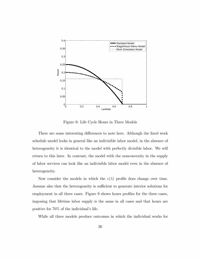
Figure 9: Life Cycle Hours in Three Models

There are some interesting differences to note here. Although the fixed work

schedule model looks in general like an indivisible labor model, in the absence of

heterogeneity it is identical to the model with perfectly divisible labor. We will

return to this later. In contrast, the model with the nonconvexity in the supply

of labor services can look like an indivisible labor model even in the absence of

heterogeneity.

Now consider the models in which the e(λ) profile does change over time.

Assume also that the heterogeneity is sufficient to generate interior solutions for

employment in all three cases. Figure 9 shows hours profiles for the three cases,

imposing that lifetime labor supply is the same in all cases and that hours are

positive for 70% of the individual’s life.

While all three models produce outcomes in which the individual works for

26

only a fraction of his or her life, a key distinction is that in the benchmark model

the hours profile drops to zero continuously, while in the other two models the

hours profile drops to zero discontinuously. This discontinuity in the life cycle

profile for hours worked is a key distinguishing feature of the second and third

models relative to the benchmark model. Another interesting distinction has to

do with the profile for hours worked while working. In the work schedules model,

the hours profile is flat for the region in which hours are positive, but in the other

two models there is a positive relationship between hours and productivity in the

region with positive hours. In this regard the first two models are similar, while

the third is different. In terms of life cycle variation, the work schedule model

looks like a pure indivisible labor model.

3. Tax and Transfer Programs

In this section I contrast the implications of the three models for how a simple tax

and transfer program affects life cycle and aggregate labor supply outcomes. In

particular, I will consider a policy that levies a proportional tax τ on labor income

and uses the proceeds to fund a lump-sum transfer to all individuals currently

alive, subject to a balanced budget constraint. This simple policy has been studied

extensively in the literature on cross-country differences in hours of work and

serves as a useful benchmark for contrasting the implications of these three models.

27

3.1. Analytic Results

It is easy to derive the implications of such a tax policy on the optimal labor

supply choices of individuals. Recall that given the specification of the model we

can interpret the changes in the individual choices as reflecting changes in the

steady state equilibrium. In the case of the benchmark model, the first order

condition that determines the optimal choice of h(0) becomes:

(1− τ)e(0)

[(1− τ)R 10h(λ)e(λ)dλ] + T

= v0(1− h(0)) (3.1)

The condition that relates h(λ) to h(0) is unchanged, since the tax rate affects

these choices in the same fashion:

v0(1− h(λ))

v0(1− h(0))=

e(λ)

e(0)(3.2)

The government budget constraint implies that:

τ

Z 1

0

h(λ)e(λ)dλ = T (3.3)

Combining the government budget constraint into the first order condition for

h(0) gives:(1− τ)e(0)R 10h(λ)e(λ)dλ

= v0(1− h(0)) (3.4)

Because the solution for h(λ) as a function of h(0) is unchanged, it follows that

the solution for h(0) is decreasing in τ .

28

Similar calculations can be done for the other two models. In both cases, taxes

do not distort the conditions that relate optimal choices along the intensive and

extensive margins. The reason is that both of these margins are distorted by taxes

in the same fashion, so that the distortions cancel. In terms of a diagrammatic

exposition, this implies that the upward sloping curve that relates optimal choices

of intensive and extensive margins does not shift in response to a change in the

tax and transfer system. But the tax and transfer scheme does distort the con-

dition that relates total amount of time spent working to the marginal utility of

consumption. This leads to a downward shift in the downward sloping relation.

It follows that in both cases an increase in the scale of the tax and transfer sys-

tem leads to a decrease in hours worked along both the intensive and extensive

margins.

It is also instructive to contrast the implications of the three models for the case

in which there is no heterogeneity. In this case, it is easy to show that the bench-

mark model and the work schedule model will imply that all adjustment takes

place along the intensive margin, whereas the nonconvex labor services model

implies that all of the adjustment takes place along the extensive margin.

3.2. Numerical Examples

In this subsection I solve some numerical examples to further explore the responses

studied analytically in the previous subsection. In order to do this one needs to

choose functional forms and parameter values. I choose the standard form for the

29

choice of the utility from leisure function:

v(1− h) =α

1− 1γ

(1− h)1−1γ

I also assume that u(c) is given by log c. This corresponds to the standard as-

sumption in most aggregate analyses, that preferences are consistent with balanced

growth. The appropriateness of this assumption in terms of matching individual

level trends in hours worked is somewhat of an open question. While this as-

sumption is important for the level of the effects that I report, it is not likely

to be of first order importance in terms of the relative findings across the three

specifications.

For the life cycle productivity profile I choose the quadratic specification:

e(λ) = 1− p0λ2

Note that with log utility over consumption, the labor supply profile is invariant to

proportional shifts in the productivity profile, so that there is no loss in generality

in assuming λ(0) = 1.

My main objective here is to examine the relationship between the value of γ

and the resulting effects of a change in taxes. As a result I will consider several

different values of γ. Because the analysis of the work schedules model is the novel

contribution of this paper, I will focus on this model when choosing parameter

values. As noted earlier, the solution to this model will involve two values: the

fraction of time devoted to work when working, and the fraction of life devoted to

30

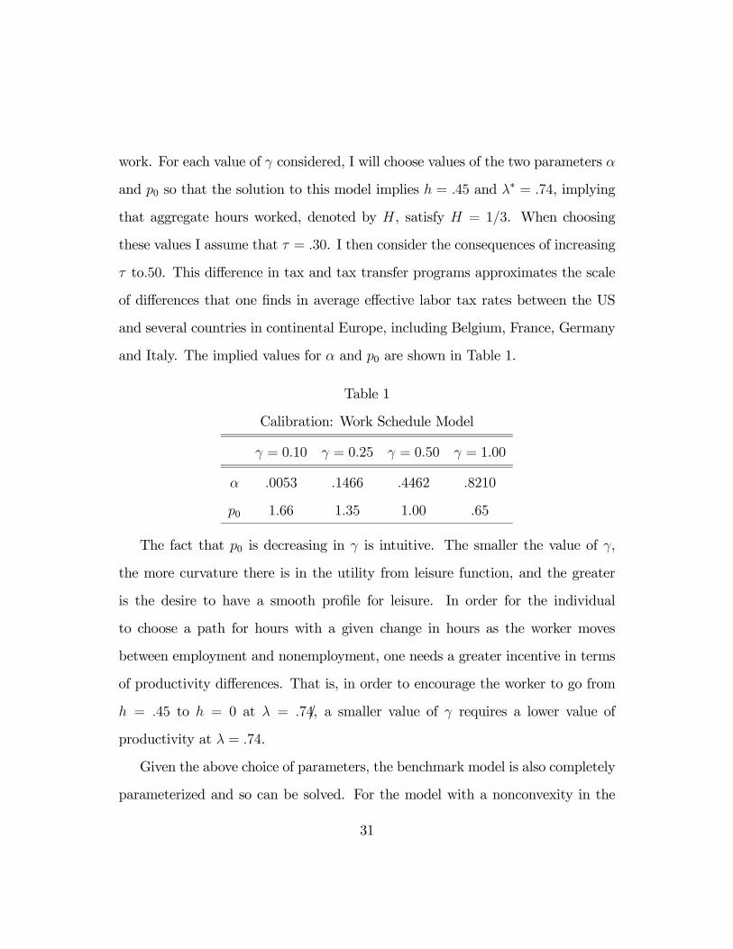
work. For each value of γ considered, I will choose values of the two parameters α

and p0 so that the solution to this model implies h = .45 and λ∗ = .74, implying

that aggregate hours worked, denoted by H, satisfy H = 1/3. When choosing

these values I assume that τ = .30. I then consider the consequences of increasing

τ to.50. This difference in tax and tax transfer programs approximates the scale

of differences that one finds in average effective labor tax rates between the US

and several countries in continental Europe, including Belgium, France, Germany

and Italy. The implied values for α and p0 are shown in Table 1.

Table 1

Calibration: Work Schedule Model

γ = 0.10 γ = 0.25 γ = 0.50 γ = 1.00

α .0053 .1466 .4462 .8210

p0 1.66 1.35 1.00 .65

The fact that p0 is decreasing in γ is intuitive. The smaller the value of γ,

the more curvature there is in the utility from leisure function, and the greater

is the desire to have a smooth profile for leisure. In order for the individual

to choose a path for hours with a given change in hours as the worker moves

between employment and nonemployment, one needs a greater incentive in terms

of productivity differences. That is, in order to encourage the worker to go from

h = .45 to h = 0 at λ = .7 /4, a smaller value of γ requires a lower value of

productivity at λ = .74.

Given the above choice of parameters, the benchmark model is also completely

parameterized and so can be solved. For the model with a nonconvexity in the

31

supply of labor services, there is one additional parameter h. For this model I

fix p0 = .65 and then choose h and α so as to achieve the values λ∗ = .74 and

H =Rh(λ)dλ = 1/3. For the four different values of γ in Table 1, the implied

values of h are given by .037, .13, .25, and .37 as γ increases from .10 to 1. Similar

to the relation observed above, the greater the curvature in the utility from leisure

function, the greater the nonconvexity must be in order to generate a solution in

which the extensive margin is operative.

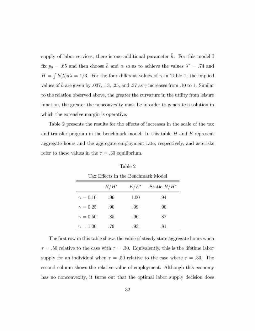
Table 2 presents the results for the effects of increases in the scale of the tax

and transfer program in the benchmark model. In this table H and E represent

aggregate hours and the aggregate employment rate, respectively, and asterisks

refer to these values in the τ = .30 equilibrium.

Table 2

Tax Effects in the Benchmark Model

H/H∗ E/E∗ Static H/H∗

γ = 0.10 .96 1.00 .94

γ = 0.25 .90 .99 .90

γ = 0.50 .85 .96 .87

γ = 1.00 .79 .93 .81

The first row in this table shows the value of steady state aggregate hours when

τ = .50 relative to the case with τ = .30. Equivalently, this is the lifetime labor

supply for an individual when τ = .50 relative to the case where τ = .30. The

second column shows the relative value of employment. Although this economy

has no nonconvexity, it turns out that the optimal labor supply decision does

32

entail an interval with zero hours. The last column shows the implication for

aggregate hours in a model that assumed a constant value of productivity over

the life cycle. In this case the employment rate is always equal to one and there

is no adjustment along the extensive margin. The results in this table should not

come as a surprise to anyone familiar with this type of exercise. There is a strong

positive relationship between the effect of a tax/transfer on steady state hours

and the value of γ. When γ = 1.00 the effect of an increase in the labor tax rate

of twenty percentage points leads to an decrease in hours of work of roughly 20

percent. In contrast, when γ = .10, the effect is only about one-fifth as large.

The effect of heterogeneity on this result is relatively small. One point of interest

in this table is that even in the context of this model, one can obtain a response

along both the intensive and extensive margins. As the second column shows,

when γ is large, there is a significant change along the extensive margin. But

when γ is small, this response disappears.

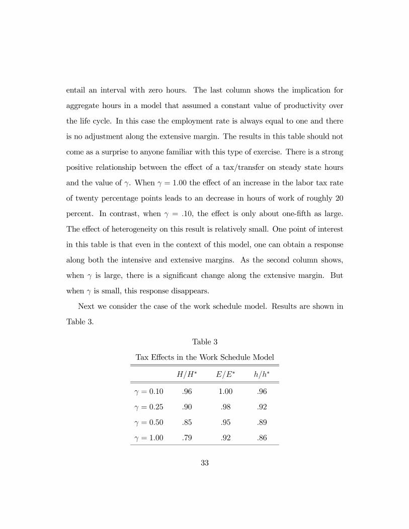
Next we consider the case of the work schedule model. Results are shown in

Table 3.

Table 3

Tax Effects in the Work Schedule Model

H/H∗ E/E∗ h/h∗

γ = 0.10 .96 1.00 .96

γ = 0.25 .90 .98 .92

γ = 0.50 .85 .95 .89

γ = 1.00 .79 .92 .86

33

The key result that emerges from this table is that both the aggregate response

and the breakdown of this response into intensive and extensive margins is iden-

tical to that in the benchmark model. We postpone further discussion until we

have presented results for the model with the nonconvexity in the supply of labor

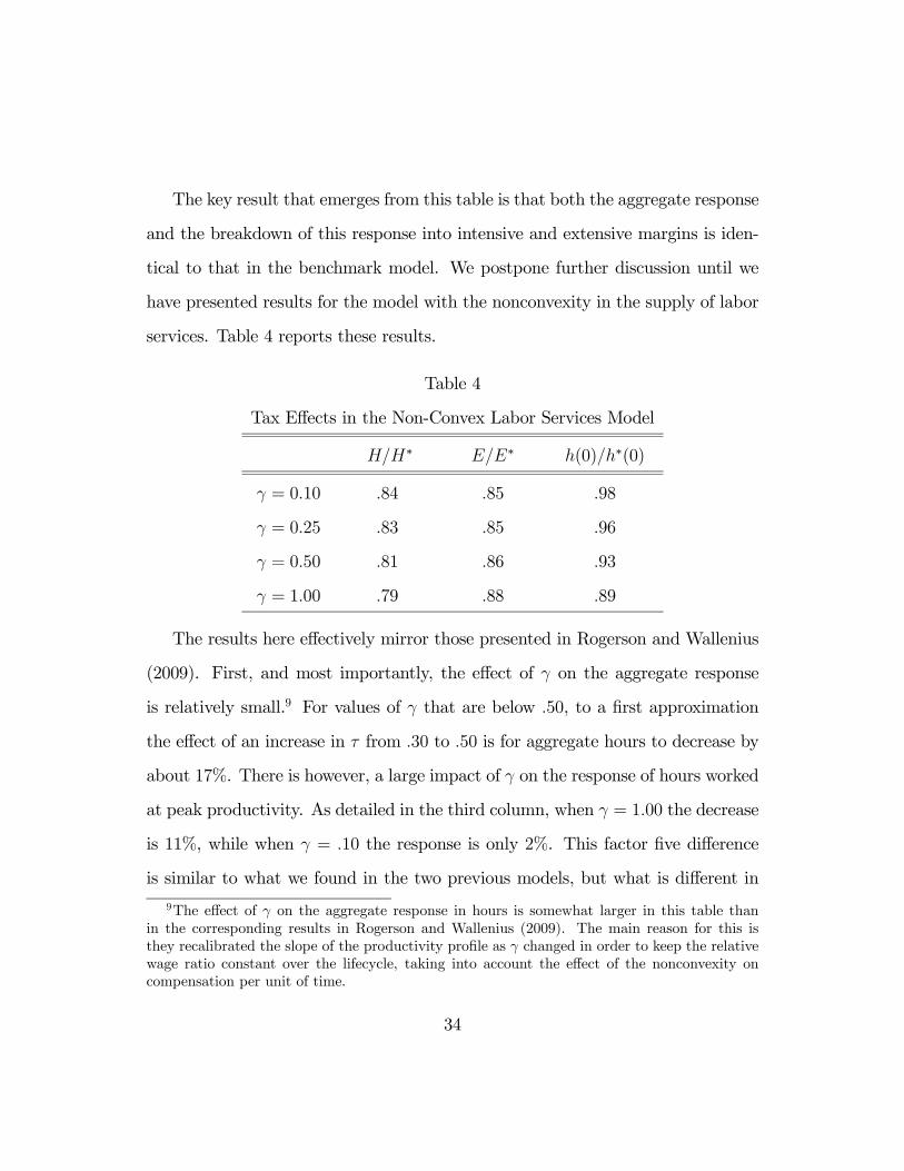
services. Table 4 reports these results.

Table 4

Tax Effects in the Non-Convex Labor Services Model

H/H∗ E/E∗ h(0)/h∗(0)

γ = 0.10 .84 .85 .98

γ = 0.25 .83 .85 .96

γ = 0.50 .81 .86 .93

γ = 1.00 .79 .88 .89

The results here effectively mirror those presented in Rogerson and Wallenius

(2009). First, and most importantly, the effect of γ on the aggregate response

is relatively small.9 For values of γ that are below .50, to a first approximation

the effect of an increase in τ from .30 to .50 is for aggregate hours to decrease by

about 17%. There is however, a large impact of γ on the response of hours worked

at peak productivity. As detailed in the third column, when γ = 1.00 the decrease

is 11%, while when γ = .10 the response is only 2%. This factor five difference

is similar to what we found in the two previous models, but what is different in

9The effect of γ on the aggregate response in hours is somewhat larger in this table thanin the corresponding results in Rogerson and Wallenius (2009). The main reason for this isthey recalibrated the slope of the productivity profile as γ changed in order to keep the relativewage ratio constant over the lifecycle, taking into account the effect of the nonconvexity oncompensation per unit of time.

34

this model is that at the same time that decreasing γ leads to a decrease in the

response along the intensive margin, it leads to an increase in the response along

the extensive margin.

4. Discussion

The main result that I want to focus on is the very dramatic difference between

the work schedule model and the nonconvex labor services model. First and

foremost, the work schedule model implies that the aggregate response is very

sensitive to the value of the preference parameter γ, while the nonconvex labor

services model implies much less sensitivity. For the specifications considered,

the two models generate similar responses in aggregate hours when γ = 1, but

when γ = .10 the response in the nonconvex labor services model is roughly four

times as large. However, what is striking about these two different cases is that

if one looks only at the life cycle profiles for the two cases, then one finds in both

cases that in terms of life cycle labor supply almost all of the variation comes

from the extensive margin. In particular, consider the case in which γ = .10 and

the numerical specifications from the previous section. In the case of the work

schedules model, by assumption there is no change along the intensive margin for

an individual who remains in employment over the life cycle. In the case of the

nonconvex labor services model, the range of work along the intensive margin for

an individual over their life cycle is from .433 to .457. So both of these models

are consistent with the observation in the US data that annual hours of work vary

relatively little for full time employed males over the life cycle, with most of the

35

variation having to do with changes from either full time to nonemployment, or

full time to part time. (See, e.g., Prescott et al (2009) for evidence on this point.)

However, despite this fact, the two models have dramatically different implications

for the magnitude of the response in aggregate hours to a change in the scale of

the tax and transfer program.

Loosely speaking, one might view these two models as two different models

that give rise to something that looks like a pure indivisible labor model, where

by a pure indivisible labor model I have in mind a model that takes the intensive

margin as fixed exogenously. Such a model has two striking implications. First,

the aggregate labor supply response to changes in the scale of tax and transfer

programs is large, and second, the aggregate response in hours worked is indepen-

dent of the curvature parameter on the utility from leisure function. One might

conjecture that any underlying model that generates something that looks like

the pure indivisible labor model in steady state might have these same implica-

tions. The nonconvex labor services model analyzed by Prescott et al (2009) and

Rogerson and Wallenius (2009) is one example for which this conjecture is true.

However, the very simple work schedule model analyzed in this paper shows

that this conjecture is not generally true. That is, the mere fact that the extensive

margin is the key margin of adjustment in terms of labor supply over the life cycle

need not imply that aggregate responses are large or that the preference parameter

dictating curvature in the utility from leisure function is irrelevant. In fact, despite

the fact that the work schedules model implies that all adjustment over the life

cycle takes place along the extensive margin, we found that aggregate hours in

36

this model behaved virtually identical to how they behave in a model that has all

life cycle adjustment take place along the intensive margin. One simple conclusion

from the above discussion is that the implications of indivisible labor for aggregate

labor supply depend very much on what the underlying source of the apparent

indivisibility is.

The above discussion cautions us that just because the extensive margin is

dominant in terms of individual labor supply changes over the life cycle, we should

not conclude that the curvature parameter in the utility from leisure function is

irrelevant for understanding the response of aggregate hours to various changes

in the economic environment. But the work schedule model also has important

implications regarding what information is needed to obtain estimates of the cur-

vature parameter γ. In particular, one might argue that micro data provides the

best opportunity to learn about preference parameters because individuals are

subjected to many large changes in the factors that shape their economic envi-

ronment. Coupled with the fact that micro data sets give us observations on a

relatively large number of individuals, it follows that this source provides us with

lots of independent observations on how individuals respond to large changes in

their economic environment. But the simple model of work schedules that I have

sketched out implies that idiosyncratic variation is irrelevant to the determination

of the work schedules. That is, if we were to simply change the tax rate that a

given individual faces, as opposed to the tax rate that all individuals face, then

nothing would happen to the economy wide choice of work schedules and the in-

dividual decision problem would look just like a pure indivisible labor problem.

37

Even observing the entire lifetime labor supply response of a given individual to

a particular change in their economic situation would not allow us to uncover the

value of γ.

To pursue this a bit further, consider an individual who is near the point of

peak life cycle productivity, and observe how this individual responds to an unan-

ticipated change in the return to work at this point in time. If the unanticipated

change leads to higher returns to work, there is no option for the individual to

increase his or her hours of work, so we will necessarily not observe any change in

hours of work in response to this event. One might falsely conclude that individ-

uals are not very willing to substitute leisure, either across time or in return for

additional consumption. Alternatively, suppose that the effect of the change is to

reduce the return to work. If the period being considered is close to peak produc-

tivity, then in order for the change to bring about a change in hours worked at

that point would require a sufficiently large change in the return to work to lower

the return below that of the reservation productivity level e(λ∗). It follows that

except for very large changes we would again observe no change for this individ-

ual. In either case, looking at contemporaneous responses at the individual level

to idiosyncratic changes in the return to working would lead us to find effectively

no response in hours worked. Yet the same change in the return to working, when

relevant for all individuals might lead to a large change in aggregate hours worked.

The key point is that despite the wealth of changes that take place at the micro

level, it may be that the responses of individuals to aggregate changes in the eco-

nomic environment may play a key role in helping us uncover the key parameters

38

of individual preferences. Put somewhat differently, the results in Chang and Kim

(2006) show us that given a fixed working length per period, micro data on hours

and wages does not provide information on the parameter γ.

At this point it is useful to remark on some of the features of the very simple

work schedule model considered here. The work schedule model studied here is

really nothing more than an example that can (hopefully) be useful in illustrat-

ing some basic points. But as a serious model that might be used to provide

compelling guidance to either data analysis or the response of hours worked to

policy changes it undoubtedly raises some basic questions. First, taking as given

that one of the most robust patterns in the micro data is the increasing profiles

for wages and annual hours worked over the life cycle, an important limitation

of the work schedule model studied here is that it does not account for the in-

crease in annual hours worked over the life cycle. One generalization of the model

considered here that could address this issue would be to allow for the possibil-

ity that as individuals accumulate experience they perform different roles within

an organization, and that some of these roles might require a different number

of hours. For example, when an individual gets promoted from being a regular

worker to being a supervisor, maybe he or she has to show up for work earlier

and stay later in order to facilitate the opening and closing of the establishment.

The key point is that a work schedules model may incorporate the reality that

different positions may be associated with different hours, with these differences

reflecting factors from the production side. That is, even if wages and hours move

together, the variation might be determined solely by features of production, and

39

so not provide any information about preferences aside from the obvious revealed

preference implication.

A second issues concerns the economy wide nature of the work schedule. While

one might accept the fact that a given establishment must choose a work sched-

ule that coordinates the working hours of its employees, it is somewhat less clear

that this needs to be done across establishments. One might then expect to see

different establishments with different work schedules, each one reflecting the de-

sired work hours for different subsets of the population. In the simple model that

I studied, this might seem a reasonable solution to the problem. But there are

three issues to raise. First, it seems reasonable that for many establishments,

it is important to understand that an important attribute of the business is its

hours of operation, and that it is important to be available to deal with customers

during what are perceived to be “usual” or “normal” business hours. Second, to

the extent that establishments care about turnover, it is important to incorpo-

rate the potential productivity losses associated with solutions that would involve

individuals moving across establishments whenever there was a change in their

desired hours of work. Third, to the extent that there are some frictions in labor

markets, establishments may need to take into account the work preferences of

the “average” worker when creating a position.

Having raised these issues, it is of course also true that there are some differ-

ences in work schedules across establishments within industries, as well as across

occupations or industries. Teachers have annual work schedules that are far dif-

ferent from many other occupations. It is plausible that this plays a role in the

40

decision of some individuals whether to enter that occupation. But it is more

likely that the selection relevant for this choice has to do with permanent dif-

ferences in preferences as opposed to life cycle changes in the return to working.

There are also many jobs in which coordination of work schedules is viewed as less

important. Many restaurants and retail establishments hire a mix of full and part

time workers. For certain subsets of the population these opportunities are likely

to be quite important and effectively create a situation in which the worker faces

a flexible hours choice at a given wage. Even in a world in which many jobs have

fixed work schedules, an individual can always augment his or her hours of work

by taking on an additional job from a sector that offers opportunities with flexible

hours. The simple model that I considered assumed that such possibilities do

not exist. Understanding both the extent of the availability of such opportunities

and how they influence our inference about labor supply is an important issue for

future research.

5. Conclusion

I analyze three different models of life cycle labor supply. The first is the standard

model that features only a choice of hours along the intensive margin. The other

two both feature operative choices along both the intensive and extensive margin,

but they differ in terms of the underlying economic reason for the operative choice

along the extensive margin. The first assumes that individuals face different wage

rates per unit of time depending upon the amount of time devoted to work. The

second assumes that all work must be coordinated across individuals, implying

41

that all individuals must work the same amount of time. Qualitatively these two

models look similar, in that both can generate life cycle labor supply profiles in

which adjustment along the extensive margin is the key margin of adjustment. I

then show that these two models have very different implications for how aggregate

labor supply responds to changes in the scale of a simple tax and transfer scheme.

In the first model, curvature in the utility from leisure function plays relatively

little role in determining the overall change in aggregate hours worked, whereas

in the second case this parameter is of first order importance. It follows that an

operative extensive margin need not imply that this curvature is irrelevant for

aggregate labor supply responses. However, I also argue that the second model

has important implications for what data is most able to provide evidence on the

extent of curvature in the utility from leisure function. In particular, panel micro

data that is dominated by idiosyncratic variation in the key forcing factors may

not of much use. Instead, one may want to find forcing variables which feature

aggregate variation.

The analysis presented here has focused on some very simple settings in order

to best communicate the messages just repeated above. An important task for

future work is to examine the extent to which these messages are robust to settings

that are more closely connected to the data. The two models analyzed here

represent extensions of the canonical labor supply model in which the constraint

set facing the individual is altered. In the standard model, the one-period budget

constraint is linear in hours worked. In the model with a wage-hours menu,

the one period budget constraint is non-linear. In the work schedules model it

42

is represented by two disjoint points. A basic message of the analysis is that

the nature of the constraint set matters both for inferring parameter values of

individual utility functions and for the aggregate response to a given change in

the overall economic environment. But the models studied here are very simple

and extreme prototypes that hopefully capture some component of the constraints

that individuals face. An important issue to consider more general versions of

these features and to assess the quantitative significance of each of them. For

example, even if hours at a particular employer are fixed from the perspective

of an individual worker, there are other employers that may offer different hours

of work. Important issues then involve the extent to which this individual can

locate these other opportunities (i.e., are there search frictions) and the extent

to which the worker’s skills are transferable across employers (i.e., the nature of

human capital). There may also be opportunities for working on a second job if

the worker wishes to increase his or her hours of work. One would then need to

incorporate the form that these opportunities take. The effect of possible market

imperfections on constraint sets is also relevant, as is the nature and extent of

human capital accumulation. Finally, in the context of models with uncertainty,

there are important issues about the nature of uncertainty and the information

sets of individual agents. While some work along these lines has been carried out,

there are still many issues to be resolved, specifically in assessing the importance

of these various features for the properties of aggregate labor supply.

43

References

[1] Aaronson, D., and E. French, “The Effect of Part-Time Work on Wages:

Evidence from the Social Security Rules,” Journal of Labor Economics 22

(2004), 329-352.

[2] Aiyagari, R., “Uninsured Idiosyncratic Risk and Aggregate Savings,” Quar-

terly Journal of Economics 109 (1994), 659-683.

[3] Altonji, J., “Intertemporal Substitution in Labor Supply: Evidence from

Micro Data,” Journal of Political Economy 94 (1986), S176-S215.

[4] Altonji, J., and C. Paxson, “Labor Supply Preferences, Hours Constraints,

and Hours-Wage Trade-offs,” Journal of Labor Economics 6 (1988), 254-276.

[5] ____________________, “Labor Supply, Hours Constraints and

Job Mobility,” Journal of Human Resources 27 (1992), 256-278.

[6] Bell, L., and R. Freeman, “The Incentive for Working Hard: Explaining

Hours Worked Differences in the US and Germany,” Labour Economics 8

(2001), 181-202.

[7] Biddle, J., “Intertemporal Substitution and Hours Restrictions,” Review of

Economics and Statistics 70 (1988), 347-351.

[8] Biddle, J., and G. Zarkin, “Choice Among Wage-Hours Packages: An Em-

pirical Investigation of Male Labor Supply,” Journal of Labor Economics 7

(1989), 415-437.

44

[9] Browning, M., L. Hansen and J. Heckman, “Micro Data Analysis and General

Equilibrium Models,” Handbook of Macroeconomics, 1998.

[10] Chang, Y., and S. Kim, “From Individual to Aggregate Labor Supply: A

Quantitative Analysis Based on a Heterogeneous Agent Macroeconomy,” In-

ternational Economic Review 47 (2006), 1-27.

[11] __________________, “Heterogeneity and Aggregation in the La-

bor Market: Implications for Aggregate Preference Shifts,” American Eco-

nomic Review, 2007.

[12] Dickens, W. and S. Lundberg, “Hours Restrictions and Labor Supply,” In-

ternational Economic Review 34 (1993), 169-192.

[13] Domeij, D., and M. Floden, “The Labor Supply Elasticity and Borrowing

Constraints: Why Estimates Are Biased,” Review of Economic Dynamics 9

(2006), 242-262.

[14] French, E., “The Effect of Health, Wealth and Wages on Labour Supply and

Retirement Behavior," Review of Economic Studies 72 (2005), 395-427.

[15] Ham. J., “Estimation of a labor Supply Model with Censoring Due to Unem-

ployment and Underemployment,” Review of Economic Studies 49 91982),

335-354.

[16] Hansen, G., “Indivisible Labor and the Business Cycle,” Journal of Monetary

Economics 16 (1985), 309-337.

45

[17] Heckman, J., “Comments on the Ashenfelter and Kydland Papers,”

Cargnegie-Rochester Conference Series on Public Policy 21 (1984), 209-224.

[18] __________, “What Has Been Learned About Labor Supply in the Past

Twenty Years?,” American Economic Review 83 (1993), 116-121

[19] Heckman J., and T. MaCurdy, “A Life Cycle Model of Female Labour Sup-

ply,” Review of Economic Studies 47 (1980), 47-74.

[20] Huggett, M., “The Risk-Free Rate in Heterogeneous-Agent Incomplete-

Insurance Economies,” Journal of Economic Dynamics and Control 17 (1993),

953-969.

[21] Imai, S., and M. Keane, “Intertemporal Labor Supply and Human Capital

Accumulation,” International Economic Review 45 (2004), 601-641.

[22] Kahn, S., and K. Lang, “The Effect of Hours Constraints on Labor Supply

Estimates,” Review of Economics and Statistics 73 91991), 605-611.

[23] Keane, Michael, and Kenneth Wolpin, “The Effect of Parental Transfers and

Borrowing Constraints on Educational Attainment,” International Economic

Review 42 (2001), 1051-1103.

[24] Krusell, P., and T. Smith, “Income and Wealth Heterogeneity in the Macro-

economy,” Journal of Political Economy 106 (1998). 867-896.

[25] Krusell, P., T. Mukoyama, R. Rogerson, and A. Sahin, “A Three State Model

of Worker Flows in General Equilibrium,” Working Paper, NBER, 2009a.

46

[26] ___________________________________________,

“Aggregate Labor Market Outcomes: The Role of Choice and Chance,”

Working Paper, NBER, 2009b.

[27] Kydland, F., “Labor Force Heterogeneity and the Business Cycle,” Carnegie

Rochester Conference Series on Public Policy 21 (1984), 173-208.

[28] Kydland, F., and E. Prescott, “Time to Build and Aggregate Fluctuations,”

Econometrica 50 (1982) 1345-1370.

[29] Low, H., C. Meghir, and L. Pistaferri, “Employment Risk and Wage Risk

over the Life Cycle,” forthcoming, American Economic Review, 2009.

[30] Lundberg, S., “Tied Wage-Hours Offers and the Endogeneity of Wages,”

Review of Economics and Statistics 67 (1985), 405-410.

[31] Lucas, R., and L. Rapping, “Real Wages, Employment, and Inflation,” Jour-

nal of Political Economy 77 (1969), 721-754.

[32] MaCurdy, T., “An Empirical Model of Labor Supply in a Life Cycle Setting,”

Journal of Political Economy 89 (1981), 1059-1085.

[33] Moffitt, Robert, “The Estimation of a Joint Wage-Hours Labor Supply

Model,” Journal of Labor Economics 2 (1984), 550-566.

[34] Prescott, E., R. Rogerson, and J. Wallenius, “Lifetime Aggregate Labor Sup-

ply with Endogenous Workweek Length,” Review of Economic Dynamics,

2009.

47

[35] Rogerson, R., “Indivisible Labor, Lotteries and Equilibrium” Journal of Mon-

etary Economics 21 (1988), 3-16.

[36] Rogerson, R., and J. Wallenius, “Micro and Macro Elasticities in a Life Cycle

Model with Taxes,” NBER Working Paper #13017, 2007.

[37] _________________________, “Micro and Macro Elasticities

in a Life Cycle Model with Taxes,” forthcoming, Journal of Economic Theory

2009.

[38] Sousa-Poza, A., and F. Henneberg, “Work Attitudes, Work Conditions and

Hours Constraints, An Explorative, Cross-National Analysis,” Labour 14

92003), 351-372.

48