‘india’s ghg emissions profile: results of five climate modelling studies’

Results of Five Climate Modelling StudiesGHG Emissions Profile

INDIA’S

Climate Modelling Forum, India

Supported by

Ministry of Environment and ForestsGovernment of India

September 2009

Climate Modelling Forum, IndiaSupported by

Ministry of Environment and ForestsGovernment of India

September 2009

Results of Five Climate Modelling StudiesGHG Emissions ProfileINDIA’S

‘The Climate Modelling Forum consists of several independent research institutions, e.g.,NCAER, TERI, IRADe, and Jadavpur University who have received support from the Ministryof Environment & Forests, Government of India for their research work. McKinsey & Co andTERI have agreed to lend their inputs to the Forum for a comparative study of their independentmodelling results. The results and ideas expressed are those of the authors and are notattributable to the Government of India.’

Foreword

I am pleased to introduce the Report: “India’s GHG Emissions Profile: Results of Five ClimateModelling Studies”.

India has been working on the issue of its Greenhouse Gas (GHG) emissions over the previousmany years. A major study in this direction was the 2006 Report of the Expert Committee on India’sIntegrated Energy Policy, which estimated the carbon dioxide generation profile of India’s energysector up to 2031-32 under 11 different scenarios of fuel mix. India’s Ministry of Environment &Forests has also been supporting a number of organizations undertaking studies on India’s GHGemissions profile. These institutions include The Energy & Resources Institute (TERI), the NationalCouncil of Applied Economic Research (NCAER), Integrated Research and Action for Development(IRADe), and Jadavpur University. McKinsey and Company have also been doing a separate studyon this subject. This Report brings together the results of the work of these institutions, a total of fiveseparate studies. These studies are independently undertaken, and use different models, techniquesand assumptions. The Ministry’s role has been to serve as a platform to bring together the studiesand facilitate a rigorous academic peer review process. The effort has been to ensure thatthese studies are fact-based and objective and are not seen as a “government study”. We believethat the debates and negotiations on climate change are best served by rigorous and non-partisananalyses of GHG emissions profiles.

One of the interesting findings of this Report is that there is a broad convergence across the fivestudies in the estimates of India’s aggregate GHG emissions and per capita GHG emissions overthe next two decades. As these studies indicate, India’s aggregate and per capita emissions over thenext two decades will remain quite modest. The per capita GHG emissions of India (average acrossthe five studies) are estimated to be 2.1 tonnes of CO2e1 in the year 2020, and 3.5 tonnes of CO2ein the year 2030. For the sake of comparison, it is notable that the estimated per capita emissionsof India in 2020 are expected to be well below those of the developed countries, even if thedeveloped countries were to take ambitious emission reduction targets (25-40%) as recommendedby the Intergovernmental Panel on Climate Change (IPCC) for the mid-term.

jkT; ea=h ¼Lora= izHkkj½i;kZoj.k ,oa ouHkkjr ljdkj

MINISTER OF STATE (INDEPENDENT CHARGE)ENVIRONMENT & FORESTS

GOVERNMENT OF INDIA

1 Carbon Dioxide equivalent

JAIRAM RAMESH

INDIA’S GHG Emissions Profile: Results of Five Climate Modelling Studies

The results are unambiguous. Even with very aggressive GDP growth over the next two decades,India’s per capita emissions will be well below developed country averages and much lowerthan the scenarios that have been projected by certain sections of academia in the developedcountries.

Nevertheless, we are acutely conscious of the need to address the issue of climate change and bea proactive and constructive participant in search of an agreement that is fair and equitable. India’senergy intensity of GDP has reduced from 0.30 kgoe2 per $ GDP in PPP3 terms in 1980 to 0.16kgoe per $ GDP in PPP terms. This is comparable to Germany and only Japan, UK, Brazil andDenmark have lower energy intensities in the world. Our Prime Minister has already committedthat our per capita emissions will not exceed those of the developed countries under anycircumstances.

We have a robust and comprehensive National Action Plan on Climate Change (NAPCC) in placewhich has a mix of both mitigation and adaptation measures. The Plan is being converted into alarge number of specific programmes and projects. The Missions on Solar Energy and EnhancedEnergy Efficiency under the NAPCC have recently been approved by the Prime Minister’s Councilfor Climate Change. The remaining Missions under the NAPCC will be finalized by December2009. We are engaging other countries in collaborative research, development, demonstration anddissemination of clean technologies. We have an active research programme in place which includesthe monitoring of the Himalayan Glaciers. India is also an active participant in the Clean DevelopmentMechanism (CDM), with the second highest number of projects registered for any country andestimated to offset almost 10 percent of India’s total emissions per year by 2012. Recognising thecarbon storage and sequestration potential of forests, we have given a new impetus to our forestrysector, and have more than doubled our forestry budget this year to Rs 8,300 crores (USD 1.85 Bn),which we aim to further enhance. Unlike many other developing countries, India’s forest cover isincreasing every year, and is helping neutralize annually more than 11 percent of India’s GHGemissions. A number of other initiatives have also been launched that are detailed on our website(www.envfor.nic.in).

I would welcome debate and discussion on the results of these studies. This is why detailed technicaldocumentation related to these studies is included in this Report. I hope this will generate a meaningfuland informed dialogue on the subject. I would like to thank the various institutions involved in thisstudy for their rigorous work and for cooperating in the process of putting together this jointpublication.

(JAIRAM RAMESH)

2 Kilogram of oil equivalent3 Purchasing Power Parity

A. BACKGROUND AND RATIONALE

The international debate on climate change is influenced to a significant extent by studies thatestimate the GHG emissions trajectories of the major economies of the world. These studies arebased on detailed energy-economy models that project global and region or country-wise GHGemissions. Until recently, most of these studies have been carried out in developed countries, andhave often applied assumptions and techniques that do not necessarily reflect the ground realitiesin developing countries.

With a view to develop a fact-based perspective on climate change in India that clearly reflects therealities of its economic growth, the policy and regulatory structures, and the vulnerabilities ofclimate change, the Government of India, through the Ministry of Environment & Forests, hassupported a set of independent studies by leading economic institutions. This initiative is aimed atbetter reflecting the policy and regulatory structure in India, and its specific climate changevulnerabilities. The studies, which use distinct methodologies, are based on the development ofenergy-economic and impact models that enable an integrated assessment of India’s GHG emissionsprofile, mitigation options and costs, as well as the economic and food security implications.

This publication puts together the results of Phase I of three of these studies, together with those oftwo other recent studies, which focus on estimating the GHG emissions trajectory of India for thenext two decades, using a number of different techniques1 .

B. STUDIES PRESENTED IN THIS REPORT

This report summarizes the initial results of five studies. These studies are:

1. NCAER-CGE: A computable general equilibrium (CGE) model study by India’s National Councilof Applied Economic Research (NCAER)

2. TERI-MoEF: A MARKet ALlocation (MARKAL) model study by The Energy & Resources Institute(TERI)

3. IRADe-AA: An Activity Analysis model study by the Integrated Research and Action forDevelopment (IRADe)

4. TERI-Poznan: Another MARKAL model based study by The Energy & Resources Institutepresented at the 14th Conference of Parties (COP) on Climate Change at Poznan

5. McKinsey: A detailed sector by sector analysis of GHG emissions by McKinsey and Company

Executive Summary

1 The next step will involve modelling of mitigation options and costs, as well as the economic and foodsecurity implications of climate change on India. These are under investigation and will be published insubsequent reports.


5

6


The first three studies were funded by the Ministry of Environment & Forests, Government of India.The TERI-Poznan and McKinsey studies were supported by other funding sources. All studies wereundertaken independently. The Ministry of Environment & Forests functioned as the facilitator,bringing together the various studies under a common platform, facilitating a peer review processand publishing the results.

The studies have differences in model structure, specific model assumptions and parameters, aswell as some differences in the definitions of the “Illustrative Scenario” whose results are reported.The results relate to India’s emissions profile over the next two decades.

The main results of the illustrative scenarios are in Table 1; details of the assumptions and datasources for illustrative scenarios are presented in Table 2; and details of the model methodologiesare presented in Table 3.

C. KEY RESULTS

The following key results emerge from the studies.

1. Estimates of India’s per capita GHG emissions in 2030-31 vary from 2.77 tonnes to 5.00 tonnesof CO2e

2 , with four of the five studies estimating that India’s GHG emission per capita will stayunder 4 tonnes per capita3 ,4 (see Exhibit 1). This may be compared to the 2005 global averageper capita GHG emissions of 4.22 tonnes of CO2e per capita. In other words, four out of thefive studies project that even two decades from now, India’s per capita GHG emissions wouldbe well below the global average 25 years earlier.

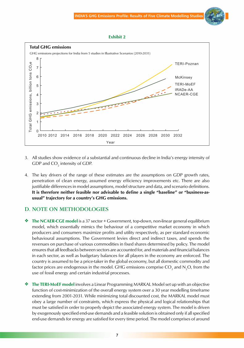
2. In absolute terms, estimates of India’s GHG emissions in 2031 vary from 4.0 billion tonnes to7.3 billion tonnes of CO2e, with four of the five studies estimating that even two decades fromnow, India’s total GHG emissions will remain under 6 billion tonnes of CO2e

3 (see Exhibit 2).

Exhibit 1

2 1 tonne of carbon is equivalent to 3.67 tonnes of CO2e3 The terminal year is 2031-32 for the TERI-MoEF and TERI-Poznan Studies.4 McKinsey study estimates include CH4 emissions from agriculture, not taken into account in the other models

Per capita GHG emissionsPer capita GHG emissions projections for India from 5 studies in Illustrative Scenarios (2010-2031)

7


Total GHG emissionsGHG emissions projections for India from 5 studies in Illustrative Scenarios (2010-2031)

3. All studies show evidence of a substantial and continuous decline in India’s energy intensity ofGDP and CO2 intensity of GDP.

4. The key drivers of the range of these estimates are the assumptions on GDP growth rates,penetration of clean energy, assumed energy efficiency improvements etc. There are alsojustifiable differences in model assumptions, model structure and data, and scenario definitions.It is therefore neither feasible nor advisable to define a single “baseline” or “business-as-usual” trajectory for a country’s GHG emissions.

D. NOTE ON METHODOLOGIES

� The NCAER-CGE model is a 37 sector + Government, top-down, non-linear general equilibriummodel, which essentially mimics the behaviour of a competitive market economy in whichproducers and consumers maximize profits and utility respectively, as per standard economicbehavioural assumptions. The Government levies direct and indirect taxes, and spends therevenues on purchase of various commodities in fixed shares determined by policy. The modelensures that all feedbacks between sectors are accounted for, and materials and financial balancesin each sector, as well as budgetary balances for all players in the economy are enforced. Thecountry is assumed to be a price-taker in the global economy, but all domestic commodity andfactor prices are endogenous in the model. GHG emissions comprise CO2 and N2O, from theuse of fossil energy and certain industrial processes.

� The TERI-MoEF model involves a Linear Programming MARKAL Model set up with an objectivefunction of cost-minimization of the overall energy system over a 30 year modelling timeframeextending from 2001-2031. While minimizing total discounted cost, the MARKAL model mustobey a large number of constraints, which express the physical and logical relationships thatmust be satisfied in order to properly depict the associated energy system. The model is drivenby exogenously specified end-use demands and a feasible solution is obtained only if all specifiedend-use demands for energy are satisfied for every time period. The model comprises of around

Exhibit 2

8


35 energy consuming subsectors and a set of conventional and non-conventional primary energysources. The technology set comprises of a detailed representation of more than 300technological options that may be adopted across the energy supply and utilization chain at theconversion, transportation, processing, and end-use application stages. Each technology isrepresented by techno-economic parameters such as its life, costs (investment, fixed and variableO&M costs), efficiency etc., which are provided as inputs to the model. The set of energycarriers consists of all the energy resources that could be available to the energy system throughindigenous production, and imports, and is described in terms of its maximum availability,associated costs at various stages and other parameters. The model projects CO2 emissionsfrom the use of fossil energy and industrial processes.

� The IRADe-AA model is a Linear Programming model, which uses the Activity Analysis frameworkto model the linkages between the national economy and environment. The model is multi-sectoral and inter-temporal and maximizes an objective function, which is the discounted sumof total consumption streams given the resources available to the economy and the varioustechnological possibilities for using them. It traces welfare effects for the low-income groups byexamining the incidence of absolute poverty in the population. Differences in consumptionpatterns among different income classes in a developing country are captured in the model.The model accounts for the behavioural responses of economic agents (such as consumersand producers) to changes in policy. The model ensures a consistent income in a number ofways, including physical flows of commodities, and the financial accounts for each type ofeconomic agent.

� The TERI-Poznan study uses the same MARKAL modelling framework as the TERI-MOEF study(see above), but with several differences in assumptions and database. First, it assumes a GDPgrowth rate of 8.2% per annum during 2001-2031, as compared to CAGR of GDP of 8.84%between 2003-2030 in the TERI-MoEF model, consistent with the GDP projections by the NCAER-CGE. Second, energy prices in TERI-Poznan were considered to evolve over the model simulationperiod as per expert judgment, whereas in the TERI-MoEF study, international energy priceswere obtained from IEAs WEO, 2007, and domestic energy prices were based on price indexesprojected by the NCAER-CGE. Third, no explicit improvements in factor productivity wereassumed in the TERI-Poznan Study, while the TERI-MoEF Study assumes a total factor productivitygrowth of 3.0% per annum in the Illustrative Scenario, which is in line with the NCAER-CGEStudy. Finally, the TERI-Poznan study considered only limited improvements in energy efficiencybased on past trends and expert judgment, whereas TERI-MoEF in the Illustrative Scenarioassumed an autonomous energy efficiency improvement of 1.5% per annum, in line with NCAER-CGE, but subject to technical feasibility limits determined through expert judgment.

� The McKinsey study estimates greenhouse gas emissions from the 10 largest emitting sectorsby 2030 based on certain assumptions of growth and energy patterns in these sectors. Theillustrative case is a bottom-up analysis of GHG emissions by sector. It assumes reasonabletechnological development across all these industries and also includes a range of mature,proven technologies. At the core of the study is an analysis of over 200 technologies (some ofwhich have been built into the illustrative case) to improve energy efficiency and reduce GHGemissions.

9


Table 1: Results for Illustrative Scenarios

GHG emissionsin 2030-31 (CO2

or CO2e) (billiontons)

Per capita GHGemissions in2030-31 (CO2 orCO2e)

CAGR of GDPtill 2030-31, %

Commercialenergy use in2030-31, mtoe

Fall in energyintensity

Fall in CO2 (orCO2e) intensity

NCAER CGEModel

4.00 billion tons ofCO2e

2.77 tons CO2eper capita

8.84%

1087 (Totalcommercialprimary energyforms)

3.85% per annum(compoundannual declinerate)

From 0.37KgCO2e to 0.15 KgCO2e per $GDP atPPP from 2003-04to 2030-31

TERI MoEFModel

4.9 billion tons (in2031-32)

3.4 tons CO2e percapita (in 2031-32)

8.84% (Exogenous– taken from CGE)

1567 (Totalcommercial energyincludingsecondary forms)in 2031-32

From 0.11 in 2001-02 to 0.06 in 2031-32 kgoe per $GDP at PPP

From 0.37 to 0.18kg CO2 per $ GDPat PPP from 2001-02 to 2031-32

IRADe AAModel

4.23 billion tons

2.9 tons CO2e percapita

7.66%(Endogenous,2010-11 to 2030-31)

1042 (Totalcommercialprimary energy)

From 0.1 to 0.04kgoe per $ GDP atPPP

From 0.37 to 0.18Kg CO2 per $GDPat PPP from 2003-04 to 2030-31

TERI PoznanMode

7.3 billion tons in2031-32

5.0 tons CO2e percapita (in 2031-32)

8.2% 2001-2031(Exogenous)

2149 (Totalcommercialenergy includingsecondary forms)in 2031-32

From 0.11 in 2001-02 to 0.08 in2031-32 kgoe per$ GDP at PPP

From 0.37 to 0.28kg CO2 per $ GDPat PPP from 2001-02 to 2031-32

McKinsey IndiaModel

5.7 billion tons(including methaneemissions fromagriculture); rangesfrom 5.0 to 6.5billion tons if GDPgrowth rate rangesfrom 6 to 9 per cent

3.9 tons CO2e percapita (2030), allGHGs

Exogenous – 7.51%(2005-2030) fromMGI OxfordEconometric model

NA

Approximately 2.3%per annum between2005 and 2030 (atPPP GDP, constantUSD 2005 prices)

Approximately 2%per annum between2005 and 2030 (atPPP GDP, constantUSD 2005 prices)

5 National Energy Map for India: Technology Vision 2030

10


Table 2: Assumptions and data sources for Illustrative Scenarios

NCAER CGEModel

TFPG = 3.0%

AEEI = 1.5%

No new GHGmitigation policy

Registrar Generalof India(till 2026,extrapolated atsame rates till2030)

InternationalEnergy Agency(WEO 2007) forinternational,endogenous fordomestic

Endogenous

Study by Bhideet.al. (2006)

National AccountsStatistics

NA

TERI MoEFModel

TFPG = 3.0%. Energyefficiency improvementconsistent with AEEIassumption incorresponding CGE runbut constrained bylimits to energyefficiencyimprovements inspecific technologies asgiven in internationalpublished literature.

No new GHGmitigation policy;discount rate = 15%,Financial Costs

Registrar General ofIndia(till 2026,extrapolated at samerates till 2030)

International EnergyAgency (WEO 2007)for international; priceindices from CGEmodel for domestic fuelprices; taxes andsubsidies included tocompute financialprices

Exogenous – from CGEoutput

NA

NA

Data set of > 300technologies1 compiledby TERI in study forPrincipal ScientificAdviser, and technologydiffusion consistentwith AEEI assumptionsas reflected in CGEmodel

IRADe AAModel

TFPG = 3.0%

AEEI = 1.5%(amounting to36.5%improvement inspecific energyconsumption from2003 to 2030).

No new GHGmitigation policy,max. savings rate =35%, Socialdiscount rate =10%, Govt. annualconsumptionincrease=9%

Registrar Generalof India(till 2026,extrapolated atsame rates till2030)

InternationalEnergy Agency forinternational;endogenous fordomestic

Endogenous

Endogenous

Max 35%

Eight electricitygenerationtechnologies(thermal, hydro,natural gas, wind,solar, nuclear,diesel, wood andmore efficient coaltechnology)

TERI PoznanModel

Efficiencyimprovements as perpast trend and as perexpert opinionconsidering level ofmaturity of specifictechnology in India.

Discount rate = 10%,Economic Costs, Nonew GHG mitigationpolicy

Registrar General ofIndia(till 2026,extrapolated at samerates till 2030)

TERI estimates forboth internationaland domestic pricesbased on prevailingmarket conditions

Exogenous – 8.2%(2001-2031)

NA

NA

Data set of > 300technologiescompiled by TERI instudy for PrincipalScientific Adviserwith recent update

McKinsey IndiaModel

Sector by sectorassumptions ofdemand andtechnology mix leadingto Illustrative scenarioemissions

Registrar General ofIndia (till 2026,extrapolated at samerates till 2030)

International EnergyAgency for internationalenergy prices

Exogenous – 7.51%(2005-2030) from MGIOxford Econometricmodel

NA

NA

Data set of 200technologiesincorporated in theMcKinsey Global CostCurve model, adaptedfor Indian volumes,capex and cost

contd…

Assumptions

Data Sources

Population

Global /domesticenergy priceprojections

GDP growthrates

ForeignSavingsprojections

Domesticsavings rate

Specific EnergyTechnologiesData

11


GHGemissionscoefficients

Various otherkey parameters

NCAER CGEModel

NationalCommunications

PublishedLiterature, NCAERand JadavpurUniversityestimates

TERI MoEFModel


Govt of India Data,other publishedliterature

IRADe AAModel


Govt of India Data

TERI PoznanModel


Govt of India Data,own estimates,expert opinion,published literature

McKinsey IndiaModel

Nationalcommunications +IPCC + own estimatesfor power sector

Govt of India data, ownestimates

contd…

Table 3: Models’ / Methodology Descriptions

NCAER CGEModel

ComputableGeneralEquilibrium

Top-down,sequentiallydynamic, non-linear, marketclearance,endogenous pricesof commoditiesand factors

TERI MoEFModel

Linear Programmingminimizing discountedenergy system cost

Bottom-up optimizationover defined period,detailed energytechnologies matrix, setof energy systemtechnical and non-technical constraints,including limits toenhancement in energyefficiency of differenttechnologies

IRADe AAModel

Linearprogrammingmaximizingdiscounted valueof consumptionover defined timehorizon

Top-downoptimizationmodel overdefined period(over 30 years with3 years for eachsequential run)with variousresource, capacityand economicconstraints

TERI PoznanModel

Linear Programmingminimizingdiscounted energysystem cost

Bottom-upoptimization overdefined period,detailed energytechnologies matrix,set of energy systemtechnical and non-technical constraintswith limits to energyefficiencyenhancement basedon past trends

McKinsey IndiaModel

Proprietary McKinseyIndia Cost Curve modelto estimate GHGemissions from the 10largest emitting sectors

Factors in estimates ofbottom upimprovements intechnology levers;analyses potential of aselected set from over200 technologies toincrease energyefficiency and reduceemissions;

Includes CO2, N2O andCH4 emissions (fromagriculture)

Demand feedbackbetween sectors:between consumingsectors and power/petroleum sectors

Model/MethodologyType

Key features ofmodel/methodology

contd…

12


NCAER CGEModel

Population, globalenergy prices,foreign capitalinflows, savingsrates, labourparticipation rates

CO2e (CO2 +N2Oweighted byGWPs) emissions,GDP, energy andCO2e intensities,final demands ofcommodities,costs of mitigationpolicies

37 productionsectors +Government

CO2 + N2O(energy andindustry only)

Coal, oil, gas,hydro, nuclear, andbiomass

TERI MoEFModel

GDP growth rates, finaldemands ofcommodities (bothfrom CGE model),global and domesticenergy prices bothconsistent with the CGEmodel), population, anddetailed technologycharacterization

CO2 emissions, energyuse patterns, energyand CO2 intensities,operating level of eachtechnology, energysystem costs,investment andmarginal costs for eachtechnology

35 energy consumingsubsectors + energysupply optionsincluding conventionaland non-conventional

CO2 (energy andindustry only)

Coal, oil, gas, hydro,nuclear, renewables,and traditional biomass

IRADe AAModel

Population, globalenergy prices,savings rates,discount rate,minimum per-capitaconsumptiongrowth rate

CO2 emissions,energy and CO2

intensities,commodity-wisedemandcategorized byend-use, income-class wisecommoditydemand, costs ofmitigation policies,poverty impacts

34 activities with25 commodities +Government

CO2 (energy,industry,households, andgovernmentconsumption only)

Coal, oil, gas,hydro, nuclear,wind, solar andbiomass

TERI PoznanModel

GDP growth ratesbased on doubling ofper capita incomesevery decade, finaldemands of energyend-use services,technologycharacterization,global and domesticenergy prices,population based onGovernmentprojections

CO2 emissions,energy use patterns,energy and CO2intensities, operatinglevel of eachtechnology, energysystem costs,investment andmarginal costs foreach technology

35 energyconsumingsubsectors + energysupply optionsincludingconventional andnon-conventional

CO2 (energy andindustry only)

Coal, oil, gas, hydro,nuclear, renewables,and traditionalbiomass

McKinsey IndiaModel

1. GDP growth rates2. Projected demandfor number of inputs(e.g., steel, power,automotive) 3.Population4. Global energy costs5. Base and non-baseload demand

Estimates IllustrativeScenario emissionsacross GHGs (CO2,N2O, CH4) over time bysector

10 sectors: Power,Cement, Steel,Chemicals, Refining,Buildings,Transportation,Agriculture, Forestry,Waste

CO2 + N2O + CH4

(energy, industry, andagriculture)

Coal, oil, gas, hydro,nuclear, wind, solar,geothermal andbiomass

Key inputs

Key outputs

Number ofsectors

GreenhouseGases included

Primary Energyforms

contd…

13


1. BACKGROUND

Anthropogenic climate change poses perhaps the most complex policy issue faced yet by the globalcommunity, moreover, one that is fraught with existential consequences for humankind at onelevel, and with major implications for the future division of global economic labour at another.Policy analysis in this field involves multidisciplinary inputs – from climate science, technology,economics, and ethics, besides international law and politics.

Mitigation of GHG emissions will, beyond a fairly modest level, involve appreciable economic coststo a society. On the other hand, the adverse impacts of climate change would be felt in diversesectors which are at the core of livelihood concerns, especially of the poor – agriculture, waterresources, coastal resources, vector borne disease, “natural” calamities, etc. Assessment of thecosts of GHG mitigation on a economy-wide basis, identifying the technologies that would need tobe deployed, and assessment of the losses from climate change impacts, or alternatively, the costsof adaptation activities, are critical inputs to climate policy-making.

Much of the global debate on climate change has been driven by the results of several types ofcomplex analytical models. In the absence of a critical mass of model based studies from India andother developing countries, the terms of the debate have tended to be driven by researchers fromthe developed countries.

With a view to making a contribution to the global debate, as well as providing such assessmentsfor national policy-making on a formal basis, using rigorous, defensible methodologies, and nationallysourced data and estimated parameters, the Ministry of Environment and Forests, Govt. of India,launched and supported a Climate Change Modeling Forum in 2006. In its present phase, theForum comprises three national economic-energy-technology models, that are partly linked, tostudy different types of policy questions on GHG mitigation.1 The models work under commonand consistent sets of assumptions, and are designed to examine alternative policy scenarios interms of their implications for the levels of energy requirements, the changes in socio-economicoutcomes, environmental impacts resulting from different energy utilization patterns, investmentrequirements, etc.

This Technical Report describes the energy-economic models developed with MoEF support, andthe results of initial simulations with these models. In addition, the results of two other studiesrecently conducted in India are also provided. Accordingly, Part I provides the detailed technicaldescriptions of the three economic models included in the climate modeling forum, as well as themodel assumptions and methodology of the two other studies conducted by other institutions. PartII furnishes the initial results of simulations involving these models and studies on the future path ofGHG emissions of the Indian economy till 2030-31/2031-32.

India’s GHG Emissions till 2030:A Compilation of Results of Five Recent Studies

1 Also under development, in respect of climate change impacts, are two linked models on water resources andagricultural crops. These two models are not further discussed in this report

14


2. PART I: TECHNICAL DESCRIPTIONS OF MODELS/METHODOLOGY:

2.1 Overview: The Models and Methodologies:

The models presently comprising the Forum are as follows:(i) India Computable General Equilibrium (CGE) Model: developed by the National Council of

Applied Economic Research (NCAER) and Jadavpur University (NCAER-CGE)(ii) India MARKAL Model: adapted from the generic version, by The Energy & Resources Institute

(TERI). (TERI-MoEF)(iii) India Activity Analysis Model: developed by Integrated Research and Action for Development

(IRADE) (IRADe-AA)

Apart from these, the two studies conducted by other institutions included in this report are:(i) Results of MARKAL model analysis by TERI (with assumptions and data distinct from TERI-

MoEF above) and presented at a side-event at the 14th Conference of Parties to the UNFCCC atPoznan in December 2008 (TERI-Poznan).

(ii) Bottom-up study by McKinsey and Co., based on the McKinsey GHG abatement cost-curve forIndia (McKinsey).

The specific features of the NCAER-CGE Model are:� A top-down macroeconomic 37 Sectors + Government, sequentially dynamic, non-linear model

with market clearance and endogenous prices of commodities and factors� Primary energy sectors are: coal, oil, gas, hydro, nuclear, and biomass; it is possible to include

(dynamic) supply constraints for each energy form� GHG emissions arise in fixed coefficients for each energy form and for specified industrial

processes such as cement manufacture� Factors of productions include: labor and capital + land for agriculture and forestry� Consumers maximize utility subject to their budget constraints, and producers maximize profits.� Armington aggregation for domestically produced and imported commodities, as well as for

different energy forms, enabling non-linear substitutions� Fixed coefficients Government expenditure, which can be varied across time periods� Technological change is described in terms of Total Factor Productivity Growth (TFPG) and

Autonomous Energy Efficiency Index (AEEI). These are exogenous model inputs� Policy variables include full set of direct and indirect taxes, subsidies, export and import taxes.

It is possible to include QRs and other policy instruments.� Outputs include: GDP (and GDP growth), outputs, prices, incomes, quantities of imports and

exports, final consumption and Government demands, besides GHG emissions.

CGE is a predictive model to simulate the effects of particular policy and parameter assumptions. Itis not a prescriptive modeling framework, and there is no economy-wide objective function.

The specific features of the TERI-MoEF model, developed on the MARKAL (MARKet Allocation)Framework are:� An energy-technology-economy linear programming model which minimizes discounted energy

system costs over a defined planning horizon to meet a vector of final demands for commoditiesand energy services

� Uses a bottom-up representation of energy producing, transforming, and consumingtechnologies. GHG emissions are by fixed coefficients for each energy technology (and cementproduction)

15


� Includes TFPG and AEEI for dynamic representation of technologies. Technological change islimited in case of each technology by considerations of feasibility based on the internationalliterature and expert opinion (energy efficiency gains are thus well short of thermodynamic limits).

� Finds a least cost set of technologies to satisfy end-use energy service demands and constraintsspecified in the defined scenario

� Outputs are resulting energy-technology combinations (feasible, optimal)� Fuel availability constraints are as per Government of India’s policies and plans� The model may be run using either economic or financial costs.

The MARKAL is a prescriptive model, and can be used to predict the future evolution of the energysector and GHGs trajectory only under the assumptions that there is in existence a central plannerfor the energy sectors whose objective function relates to minimization of discounted energy systemcosts over the simulation period, and that the exogenous parameters assumed, in particular GDPgrowth rates and rates of technological change hold true. The simulations of the TERI-MoEF MARKALmodel are coordinated with simulations of the NCAER-CGE model, and used to determine the“optimal” (in the MARKAL sense) choice of technologies for the scenarios simulated. Comparisonsbetween simulated scenarios can also provide the incremental investment costs, as well as thedifferences between the energy system costs between the scenarios.

The specific features of the IRADe Activity Analysis Model are:� The model is a “stand-alone”, non-linear, multi-sectoral, inter-temporal model which maximizes

the discounted sum of total consumption streams across the entire planning horizon, subject tospecified constraints

� A total of 25 commodities are produced using 35 production activities� Five categories of rural and five categories of urban households are included, based on per

capita consumption expenditure limits� Endogenous income distribution helps in estimating poverty in rural and urban households

This model too, is not predictive, but prescriptive, from the standpoint of a economy-wide centralplanner who seeks to maximize the discounted aggregate consumption in the economy for eachsimulation period.

Figure 1: Structure of Partially Linked Energy-Economy Models

16


While the models do not have a wired link, the outputs of the CGE model feed into the MARKALmodel. The structure of the Activity Analysis model does not lend itself to similar inputs from theCGE model. All models take population projections from the Registrar General, global energy pricesfrom International Energy Agency (IEA), and various common policy and parameter (especiallytechnological change related) assumptions.

To summarize: the NCAER-CGE, TERI-MoEF (MARKAL), and IRADe-Activity Analysis models areused to run defined Illustrative Scenarios which do not involve any new policies relevant to GHGmitigation, to determine the trajectory of GHG emissions in the economy without GHG constraintstill 2030/31.

The TERI-Poznan model uses the same MARKAL structure as the TERI-MoEF model. However, itdiverges in respect of several key assumptions and data base. For example, it assumes a lower GDPgrowth rate than the TERI-MoEF study (which draws upon the GDP projections obtained from theNCAER-CGE model). It also projects future energy prices (international and domestic) by in-houseexpert opinion, whereas TERI-MoEF uses the WEO, 2007 projections with respect to internationalenergy prices, and uses the price indices generated by the NCAER-CGE model for domestic energyprices. Finally, it is much more conservative than the Illustrative Scenario of TERI-MoEF with respectto improvements in specific energy consumption, and assumes that there is little improvement intotal factor productivity. The last set of divergent assumptions from TERI-MoEF seem to largely drivethe differences in their results for the future CO2 emissions path.

The McKinsey study employs a bottom-up approach to estimate energy use patterns in 10 sectors.It factors in bottom-up estimates of improvements from technology levers and optimizes costs bydetermining a merit order for aspplication of over 200 abatement technologies. There iscomprehensive coverage of sectors and GHGs i.e. CO2, N2O and CH4, as well as accounting fordemand feedback between consuming sectors and power/petroleum sectors. Projections of GDPgrowth are obtained from a separate global macroeconomic model .

2.2 Technical Description of the India Computable General EquilibriumModel

The CGE model developed by NCAER is used to project India’s GDP growth and GHG emissions,and to evaluate the impacts of GHG emissions abatement policies. This model is a single-countrymodel interacting with the rest-of-the-world (ROW).

2.2.1 Model StructureThis CGE model is based on a neoclassical CGE framework that includes institutional features peculiarto the Indian economy. Figure 3 depicts the building blocks of CGE model. It is multi-sectoral andrecursively dynamic. The overall structure of the model is similar to the one presented in Ghosh(1990). However, in formulating certain details of the model, such as, the income distributionmechanism a more eclectic approach is followed keeping in mind the focus on the linkages betweeninter-fossil-fuel substitutions, CO2 emissions, GDP growth and the distribution of income across therural and urban socioeconomic classes.

The model includes the interactions of producers, households, the government and the rest of theworld in response to relative prices, given certain initial conditions and exogenously given set ofparameters. Producers act as profit maximizers in perfectly competitive markets, i.e., they takefactor and output prices (inclusive of any taxes) as given and generate demands for factors so as to

17


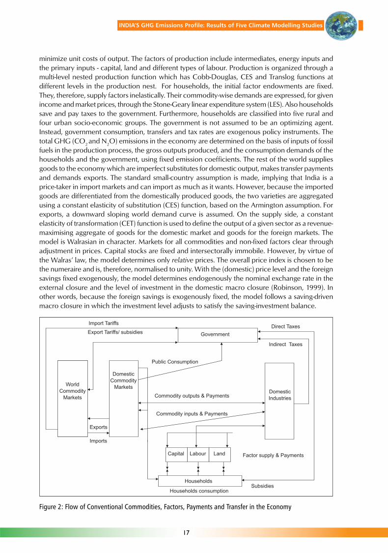
minimize unit costs of output. The factors of production include intermediates, energy inputs andthe primary inputs - capital, land and different types of labour. Production is organized through amulti-level nested production function which has Cobb-Douglas, CES and Translog functions atdifferent levels in the production nest. For households, the initial factor endowments are fixed.They, therefore, supply factors inelastically. Their commodity-wise demands are expressed, for givenincome and market prices, through the Stone-Geary linear expenditure system (LES). Also householdssave and pay taxes to the government. Furthermore, households are classified into five rural andfour urban socio-economic groups. The government is not assumed to be an optimizing agent.Instead, government consumption, transfers and tax rates are exogenous policy instruments. Thetotal GHG (CO2 and N2O) emissions in the economy are determined on the basis of inputs of fossilfuels in the production process, the gross outputs produced, and the consumption demands of thehouseholds and the government, using fixed emission coefficients. The rest of the world suppliesgoods to the economy which are imperfect substitutes for domestic output, makes transfer paymentsand demands exports. The standard small-country assumption is made, implying that India is aprice-taker in import markets and can import as much as it wants. However, because the importedgoods are differentiated from the domestically produced goods, the two varieties are aggregatedusing a constant elasticity of substitution (CES) function, based on the Armington assumption. Forexports, a downward sloping world demand curve is assumed. On the supply side, a constantelasticity of transformation (CET) function is used to define the output of a given sector as a revenue-maximising aggregate of goods for the domestic market and goods for the foreign markets. Themodel is Walrasian in character. Markets for all commodities and non-fixed factors clear throughadjustment in prices. Capital stocks are fixed and intersectorally immobile. However, by virtue ofthe Walras’ law, the model determines only relative prices. The overall price index is chosen to bethe numeraire and is, therefore, normalised to unity. With the (domestic) price level and the foreignsavings fixed exogenously, the model determines endogenously the nominal exchange rate in theexternal closure and the level of investment in the domestic macro closure (Robinson, 1999). Inother words, because the foreign savings is exogenously fixed, the model follows a saving-drivenmacro closure in which the investment level adjusts to satisfy the saving-investment balance.

Figure 2: Flow of Conventional Commodities, Factors, Payments and Transfer in the Economy

18


2.2.2 Sectoral DisaggregationThe model is based on a 37-sector disaggregation of the Indian economy. The sectoral disaggregationwas decided after much deliberation on what would be the optimal number of sectors in a trade-offbetween the theoretical requirement of having a large number of sectors differentiated on the basisof their emission intensities, and the practical compulsion of maintaining a manageable number ofsectors that would facilitate computation and policy relevant interpretations of the computed results.The list of 37-sector of the Indian economy is given in the Table 1.

Table 1: Sectoral Disaggregation in the CGE model

Code Description of Sectors Code Description of Sectors

1 PAD Paddy Rice 20 IRS Iron & Steel2 WHT Wheat 21 ALU Aluminium3 CER Cereal, Grains etc, other crops 22 OMN Other manufacturing4 CAS Cash crops 23 MCH Machinery5 ANH Animal husbandry & prod. 24 HYD Hydro6 FOR Forestry 25 NHY Thermal7 FSH Fishing 26 NUC Nuclear8 COL Coal 27 BIO Biomass9 CUP Crude Oil 28 GMN Gas Manufacture & Distribution10 NGS Natural Gas 29 WAT Water11 FBV Food & beverage 30 CON Construction12 TEX Textile & Leather 31 RTM Road Transport motorised13 WOD Wood 32 RNM Road Transport non motorised14 MIN Minerals n.e.c. 33 RLY Rail Transport15 ROL Refined Oil & Coal Prod. 34 AIR Air Transport16 CHM Chemical, Rubber & Plastic prod. 35 SEA Sea Transport17 PAP Paper & Paper prod. 36 HLM Health & medical18 FER Fertilizers & Pesticides 37 SER All other services19 CEM Cement

2.2.3 The Production StructureEach producing sector has a nested production function, with the structure of nesting being thesame across sectors. Each sector produces its gross output, employing capital, labour and anaggregation of its own and other sectors’ inputs, known as intermediate inputs. The intermediateinputs are broadly of two kinds – energy and non-energy. The different types of inputs, however,combine through differently specified production functions at the various levels in the productionnest whose diagram is shown below (Figure 4).

Note that aggregate of energy inputs, AENG, is formed through a Translog function which combinesthe five sources of energy, namely, electricity, coal, natural gas, refined oil, and biomass, whereelectricity itself is a linear aggregation of the three main sources of electricity - thermal, hydropower,and nuclear. The Translog function is used because it allows different (Allen-Uzawa) substitutionelasticities between different pairs of the aforesaid five sources of energy. The remaining non-factorinputs is referred to as the aggregate materials, AM, which represents a fixed-coefficients bundle ofinputs from the non-energy sectors. The AENG and the AM combine into aggregate non-factorinputs, ANFI, through a CES function for which only one substitution elasticity is required. Further

19


Figure 3 : The Production Nesting Diagram

Nested Production Structure

up, the ANFI, labour, capital and land (in case of agricultural sectors) are coalesced into the domesticgross output using a Translog function having different substitution elasticities for different pairs ofinputs. Note that the TL function reduces to the much simpler Cobb-Douglas form in case of unitsubstitution elasticities between the various input pairs (this does happen for a subset of the 37sectors).

Domestic gross output itself is an aggregate of its two constituents – domestic sales and exports –obtained through a CET function. Finally, at the top end of the production nest, domestic sales andfinal imports into a sector are aggregated into a composite output for that sector by making use ofa CES aggregation function.

2.2.4 Description of Model - Model Equations, Variables and ParametersThe CGE model is a system of simultaneous, nonlinear equations. The model is square in a sensethat the number of equations is equal to the number of variables. In this class of models, this is anecessary (but not a sufficient) condition for the existence of a unique solution. In our case also wehave developed a set of equations in such a way that the number of equations is equal to thenumber of endogenous variables of the model. The sets, parameters and variables appeared in theequations are described below:

Sets1. AS All Sectors

(All 37 Sectors of 2003-04 SAM)2. DOMS Sectors with Domestic Sale

(All 37 sectors of 2003-04 SAM)3. FMAT Factors of Production

(k - Capital, l - Labour, la - Land, q – Commodity Input)4. GHGS Greenhouse Gases

(CO2 – Carbon Dioxide, N2O – Nitrous Oxide)

20


5. HHSC Households Classes(rh1, rh2, rh3, rh4, rh5, uh1, uh2, uh3, uh4)

6. PFAC Primary Factors of Production(k, l, la)

7. SIMP Sectors with Imports(pad, wht, cer, cas, anh, frs, fsh, col, oil, gas, fbv, txl,wod, min, pet, chm, pap, fer, irs,alu, omn, mch, rtm, rnm, air, sea, ser)

8. SNIMP Sectors without Import(cem, hyd, nhy, nuc, bio, gmn, wat, con, rly, hlm)

9. SEXP Sectors with Exports(pad, wht, cer, cas, anh, frs, fsh, col, gas, fbv, txl, wod, min, pet, chm, pap, fer, irs, alu,cem, omn, mch, rtm, rnm, rly, air, sea, ser)

10. SNEXP Sectors without Export(oil, hyd, nhy, nuc, bio, gmn, wat, con, hlm)

11. SMANU Manufacturing Sectors(txl, wod, min, pet, chm, pap, fer, irs, alu, cem, omn, mch, con, gmn, oil)

10. SNMAN Non-Manufacturing Sectors(pad, wht, cer, cas, anh, frs, fsh, fbv, col, gas, bio, hyd, nhy, nuc, wat, rtm, rnm, rly,air, sea, hlm, ser)

11. SEN Conventional Energy Sectors(col, gas, pet, hyd, nhy, nuc, bio)

12. SMAT Material Input Supply sectors(pad, wht, cer, cas, anh, frs, fsh, oil, fbv, txl, wod, min, chm, pap, fer, irs, alu, cem,con, wat, gmn, omn, mch, rly, rtm, rnm, air, sea, hlm, ser)

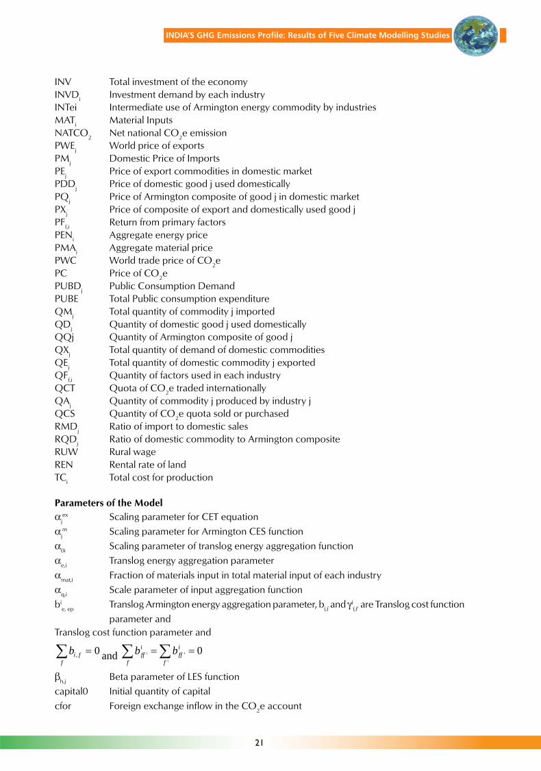
Endogenous Variables of the ModelAENi Aggregate energy inputAENCi Aggregate Energy CostsCDj Consumer Demand for Armington CommodityCO2Ci Cost for carbon emissionCO2Ei CO2 EmissionCO2Fi Quantity of CO2 offsets generated in each industryCO2Ni Net CO2 emission by each industryCO2Qi Quantity of domestic CO2 quota and offsets purchased by industriesCO2PUB Quantity of CO2 emission due to public energy useCO2PVT Quantity of CO2 emission due to private energy useCHSTKj Change in StocksDENei Quantity of domestic energy used by each industriesDHICh Disposable household incomeECi CO2 Emission CostEXR Exchange RateEPNe,i Effective price of composite energy inputsFINVi Quantity of fixed investment demand for each Armington commodityGOVI Government IncomeGDP Gross Domestic ProductHI Household incomeHICh Class wise households class wise incomeHCDh,j Households consumption demandHCEh Hoseholds Consumption ExpenditureINTj,i Intermediate input demand

21


INV Total investment of the economyINVDi Investment demand by each industryINTei Intermediate use of Armington energy commodity by industriesMATi Material InputsNATCO2 Net national CO2e emissionPWEj World price of exportsPMj Domestic Price of ImportsPEj Price of export commodities in domestic marketPDDj Price of domestic good j used domesticallyPQj Price of Armington composite of good j in domestic marketPXj Price of composite of export and domestically used good jPFf,i Return from primary factorsPENi Aggregate energy pricePMAi Aggregate material pricePWC World trade price of CO2ePC Price of CO2ePUBDj Public Consumption DemandPUBE Total Public consumption expenditureQMj Total quantity of commodity j importedQDj Quantity of domestic good j used domesticallyQQj Quantity of Armington composite of good jQXj Total quantity of demand of domestic commoditiesQEj Total quantity of domestic commodity j exportedQFf,i Quantity of factors used in each industryQCT Quota of CO2e traded internationallyQAj Quantity of commodity j produced by industry jQCS Quantity of CO2e quota sold or purchasedRMDj Ratio of import to domestic salesRQDj Ratio of domestic commodity to Armington compositeRUW Rural wageREN Rental rate of landTCi Total cost for production

Parameters of the Modelαj

ex Scaling parameter for CET equation

αjm Scaling parameter for Armington CES function

α0i Scaling parameter of translog energy aggregation functionαe,i Translog energy aggregation parameter

αmat,i Fraction of materials input in total material input of each industryαq,i Scale parameter of input aggregation functionbi

e, ep Translog Armington energy aggregation parameter, bi,f and γif,f’ are Translog cost function

parameter andTranslog cost function parameter and

0, =∑f

fib and 0'

'' ==∑∑f

iff

f

iff bb

βh,j Beta parameter of LES functioncapital0 Initial quantity of capital

cfor Foreign exchange inflow in the CO2e account

22


δjm Share parameter for j in Armington function

δjex Share parameter of CET composition function

δq,i Share parameter of commodity input aggregation function

δth Households direct taxendh,f Endowment of primary factors by households classesexpj Quantity of exports when supply price equals to world price

fdempubj Post tax structure of public demand

gsav Government savings.γh,j Gamma parameter of LES function

κi Industry wide CO2e emission permitkapi,j Capital composition parameterλi Depreciation rate

labor0 Initial quantity of labour.µ Average annual inflation ratenatnlco20 National CO2e emission

pwmj World Price of Importspwc World trade price of CO2epoph Population of each Households Class

prcl Price levelπj

m Windfall profit from importπj

ex Windfall profit from export

φe,g Coefficient of GHG emission by each energy typesr Interest raterewi Real wage

ρjex Elasticity of transformation for exports and domestics

ρq,i Commodity input aggregation functionρj

m Elasticity of substitution for j in Armington function

strh Share of households in total transfersub Subsidy ratesrh Households savings rate

sctk Share of total change in stocks in total investmentσi Elasticity between material and energy inputsσex

j Export demand price elasticity

tmj Tariff ratetej Export tax ratetai Taxes on gross output except export and import tax

tai Taxes on gross output except export and import taxθg CO2e equivalent of GHG emissiontc Carbon tax

τ Price levelϑi Investment share by industry of destinationxchj Share of sectoral change in stocks in total change in stocks

23


Equations of the Model1. Domestic price of Import Commodities.

mjjjj EXRpwmtmPM π−+= .).1( j ε SIMP

2. World price of Export Commodity.

exjjjj tePEPWE π−+= )1( j ε SEXP

3. Ratio of Import to Domestic Demandmj

j

jmj

mj

j PMPDDRMD

ρ+

⎭⎬⎫

⎩⎨⎧

⎟⎠⎞

⎜⎝⎛⎟⎟⎠

⎞⎜⎜⎝

⎛∂−

∂=

11

1 j ε SIMP ∩ DOMS

4. Demand for Imports

jjj QDRMDQM .= j ε SIMP ∩ DOMS

5. Armington Aggregation Equation

( ){ } mj

mj

mj

jmjj

mj

mjj QDQMQQ ρρρα

1

.1−−− ∂−+∂= j ε SIMP ∩ DOMS

6. Price of composite for imports and domestically used commodity

jjjjjj PDDQDPMQMQQPQ += j ε AS

7. Armington Aggregation equation for the case of no imports

jmjj QDQQ α= j ε SNIMP

8. CET equation for exports and domestic

( ){ } exj

exj

exj

jexjj

exj

exjj QDQEQX ρρρα

1

1 ∂−+∂= j ε SEXP ∩ DOMS

9. Ratio of exports and domestic demands1

1

1 −

⎭⎬⎫

⎩⎨⎧

⎟⎟⎠

⎞⎜⎜⎝

⎛∂

∂−⎟⎠⎞

⎜⎝⎛=⎟

⎠⎞

⎜⎝⎛

exj

exj

exj

j

j

j

jPDD

PEQD

QE ρ

j ε SEXP ∩ DOMS

10. Price of composite of exports and domestic commodity

jjjjjj QDPDDQEPEQXPX += j ε AS

11. CET equation for no exports

jexjj QDQX α= j ε SNEXP

12. Commodity Market Balance

ii QAQX = i ε AS

13. Average cost pricing rule for industries

( ) ii

ii TCta

PXQA =⎟⎠⎞⎜

⎝⎛

+1 i ε AS

14. Commodity Market Balance

jj QAQX = j ε AS

15. Average cost pricing rule for industries

( ) ii

ii TCta

PXQA =⎟⎠⎞⎜

⎝⎛

+1 i ε AS

24


16. Production costs for industries.

ijj

ijiff

ifi CCOPQINTPFQFTC 2.,,, ++= ∑∑ i ε ASf ε PFAC

17. Quantities of factor inputs (Translog Production Function)

i ε ASf ε FMAT

18. Commodity Inputs Aggregation Equation for Industries (cobb-Douglas Production function)

i ε ASi ε AS

19. Ratio of materials and energy inputs in aggregate commodity inputs

i ε AS

20. Price of aggregate commodity inputs faced by industries

i ε AS

21. Effective cost of aggregate of Armington energies

i ε ASe ε SEN

22. Quantity of aggregate of Armington energy inputs

i ε ASe ε SEN

23. Quantity of each type of Armington energy employed in each industry

i ε AS

e ε SEN

24. Aggregation of Non-energy commodities as Industry Intermediate inputs

i ε ASmat ε SMAT

25. Price of aggregate material input faced by industry

i ε ASmat ε SMAT

25


26. Ratio of domestic commodity to Armington composite.

i ε AS

27. Quantities of Domestic and Imported Energy of each type used as input by each industry.

j ε AS

e ε SEN

28. GHG emission by each industry in carbon equivalent

i ε AS

e ε SENg ε GHGS

29. Quantity of CO2 offsets generated in each industry

i ε AS

30. Net taxable or saleable CO2 emission by each industry

i ε AS

31. Penalty due to positive net CO2 emission by each industry.

i ε AS

32. Effective price of energy input for industry

i ε AS

e ε SENg ε GHGS

33. Effective price of capital for industry I in GE model

i ε AS

34. Effective price of labour for industry I in GE model

i ε AS

35. Effective land rental rate in each industry in GE model

i ε AS

36. Gross domestic product at factor costs

j ε AS

37. Households income by households class

i ε AS

26


38. Disposable Household income by households class h

i ε ASh ε HHSC

39. Net household income

h ε HHSC

40. Net households expenditure

h ε HHSC

41. Total government income

i ε AS

j ε ASh ε HHSC

42. Net public consumption expenditure

43. Consumer LES demand equations by households class

j ε AS

h ε HHSC

44. Consumer demand equation

j ε ASh ε HHSC

45. Public demand equationj ε AS

46. Value of gross investment in the economy

h ε HHSC

47. Investment demand by each Industryi ε AS

48. Quantity of fixed investment demand for each Armington commodity in the economy.

i ε AS

j ε AS

27


49. Quantity of change in stock demand for each Armington commodity

j ε AS

50. Total demand of Armington Composites in the Domestic market.

j ε ASi ε AS

51. Export Demands for domestic Commodities

j ε SEXP

52. Labour market balance holds for GE model

i ε AS

53. Capital market balance holds for GE model

i ε AS

54. CO2e emission due to final consumer demands for energy commodities.

j ε ASe ε SENg ε GHGS

55. CO2e emission due to final public demands for energy

j ε AS

e ε SENg ε GHGS

56. Net national CO2e emission.

i ε AS

57. Domestic CO2e balance in the economy

i ε AS

58. External CO2e balance of the National Economy

59. Price normalisation equation

j ε AS

28


2.2.5 Data and Implementation of the ModelIn the above section the system of simultaneous non-linear equations comprising the model havebeen set out. These equations are solved to determine the equilibrium values of the endogenousvariables based on the available information on exogenous variable and structural parameters. Themodel has been solved for the base year 2003-04 and, subsequently, for the future 28 years, till2030-31 with no specific GHG abatement policies Therefore to implement the model, one needsto derive estimates of the parameters of the model and the values of the exogenous variables of thesame.

The principal exogenous variables and parameters of the model are as follows:

Exogenous Variables(1) Population.(2) Foreign Savings.(3) Land Endowment in the Economy.(4) Total Labour Supply in the Economy.(5) Total Capital Stock in the Economy.(6) World Prices of Commodities.

Technological Parameters(1) Substitution Elasticities in the Production Functions.(2) Scale Parameters in the Production Functions.(3) Share Parameters in the Production Functions.(4) Emission Coefficients.

Behavioral Parameters(1) Savings Rates.(2) Demand System Parameters.(3) Share of aggregate Investment earmarked for inventory investment.(4) Shares for allocation of total inventory investment into sectoral “Change in Stocks”.(5) Share of Fixed Investment by sector of origin.

Policy Parameters(1) Tax and Tariff rates.(2) Subsidy rates.(3) Share of public consumption demand by sector of origin.

The principal data source for estimating these parameters is the 37-sector SAM. The NCAER andJadavpur University have pooled their respective efforts to construct a 37-sector SAM for the year2003-04. This SAM for the year 2003-04 helps to estimate the share parameters of our model. Thisestimation of share parameters is based on the assumption that the base-year (2003-04) values inthe SAM is represents an “equilibrium” set of values which the CGE model must replicate asclosely as possible,. This assumption of base-year equilibrium is a very useful one as it enables agreat deal of prior information on parameter estimation.

However, the SAM does not provide the data for estimating the policy parameters of our model. Toestimate these parameters data from National Accounts Statistics (NAS), Annual Survey of Industries(ASI), Public Finance Statistics of India, and various rounds data of National Sample SurveyOrganization (NSSO) have been used.

29


Knowledge of a base-year SAM and the assumption that the base year is in equilibrium does notprovide any information about the values of elasticities. Additional information and data are requiredfor estimation of these parameters. The elasticity parameters describe the curvature of variousstructural functions. The structural functions used in the CGE model are: Translog production function,Cobb-Douglas production function, LES demand function for consumers, CES import demandfunction, and CET export supply function. Estimation of values of these parameters, and in somecases by reference to the published literature was undertaken by Jadavpur University.

2.2.6 Time Path of Exogenous VariablesIt has been mentioned earlier in the description of the model that several exogenous variables thathave been used in the solving the model. To be specific, they are the following:1. Foreign Savings.2. Population.3. Land Endowment.4. Total Labour Supply in the Economy.5. World Prices of Commodities.

The sources of the data for the parameters and the exogenous variables are elaborated below.

To obtain the time series data on foreign savings the projected growth rate from the macro-econometric model for the Indian economy prepared by Bhide et.al. (2006) has been used. Thisstudy reveals that the capital inflow other than FDI and net invisibles will grow by 18 percent peryear for the next ten years i.e. 2005-06 to 2015-16. But during 2015-16 to 2025-26 this growth ratewill fall to 15 percent only for net invisibles. The FDI growth rate will move around 5 to 15 percentin different sectors for the time span 2005-06 to 2015-16. During 2015-16 to 2025-26 it will fall to 3-5 percent for different sectors. After getting the series of these variables, the series of foreign savinghas been computed with the help of the following relations.

Foreign savings (i.e.Trade balance) = (Current Account balance – Invisibles Net).Current Account Balance (i.e. C.A.B) = (Capital Account + Monetary movement).Capital account = (Foreign Direct Investment (FDI) + Capital inflow other than FDI).

The time series data on population for the time period 2003-04 to 2025-26 is available from theRegistrar General of India. A projection of the population growth rate has been made for the timeperiod 2026-07 to 2029-30. Data reveals that India’s population will increase throughout the period2003-04 to 2029-30.

To estimate the labour supply for India the data on Labour force Participation Rate (LFPR) of Indiahas been used. The National Sample Survey Organization (NSSO), in its 61st round report, givesthe same for the five years 2000-05. As per this report the usual status LFPR increased by nearly 2percentage points for males and about 3 percentage points for females during this five years timespan. This growth rate has been taken as constant throughout the time period 2003-04 to 2029-30to estimate the labour supply of India for that time period.

The total land endowment of India for the base year is available from the SAM of the year 2003-04.

The world prices are fixed at unity in the model.

2.2.7 Solution, Validation and Assumptions of the ModelThe 37-sector CGE model has been calibrated to the benchmark “equilibrium” data set of the Indian

30


economy for the year 2003-04 represented in the 37-sector SAM mentioned above. Further, usinga time series of the exogenous variables of the model, a sequence of equilibria for the 28-yearperiod from 2003-04 to 2030-31 has been generated using the General Algebraic Modeling Systems(GAMS) software. From the sequence of equilibria, the growth paths of selected (macro) variablesof the economy are outlined to describe the Illustrative Scenario.

For validation purposes, the 4-year period from 2003-04 to 2006-07 has been considered as firmmacroeconomic data is presently available only upto 2006-07. Since the model runs replicatereasonably well the actual macroeconomic magnitudes for this period, the model may be treatedas satisfactorily validated.

Finally, it must be noted that for generating the Illustrative the following key assumptions have beenmade.

Assumptions on Technological changeTotal factor productivity growth (TFPG) happens exogenously in the model. After examination ofalmost all the available empirical evidence, soliciting expert opinion and making reasoned judgementsof different baseline GDP scenarios generated for annual TFPG rate of 2, 3, and 4 percent, (coupledwith different energy efficiency growth rates) it was decided to assume an annual TFPG of 3 percentfor the Illustrative Scenario.

Improvement in specific energy consumption is incorporated in the model by making theautonomous energy efficiency improvement (AEEI) assumption used in other carbon emissionabatement models such as, GREEN (Burniaux et al, 1992) and EPPA (Babiker et al, 2001). As in theEPPA and GREEN, it is also assumed that AEEI occurs in all sectors except the primary energysectors (coal, crude petroleum and natural gas) and the refined oil sector. India has embarked on apath towards increasing energy efficiency since 1980, and its record in energy efficiency improvementin the last two decade is encouraging. Reasoned judgements on trial runs of the model have beenmade for annual AEEI growth rates of 1, 1.2, 1.4 , 1.5 and 2 (paired with different annual TFPG rates),and on this basis annual AEEI growth rate of 1.5 percent per annum has been assumed in theIllustrative Scenario, being also typical of the AEEI growth rate assumed by other modelers.

Thus, the Illustrative Scenario is based on the assumption of 3 and 1.5 percent annual growth ratesof TFPG and AEEI respectively. It should, however, be noted that while these parameter values seemto reflect recent performance of the Indian economy, there is no reason to assume that they wouldhold for the entire simulation period, and accordingly, cannot be considered as either a “baseline” or“business-as-usual” scenario.

Assumptions on Greenhouse Gas EmissionsGreenhouse gases (GHG) are emitted owing to burning of fossil fuel inputs. The major fossil fuelsused in India are coal, natural gas, refined oil and crude petroleum. In addition to GHG (CO2 andN2O) emitted by fuel combustion, there may be GHG emanating from the very process of outputgeneration. For example, the cement sector releases CO2 in the limestone calcination process.Finally, GHG emissions also result from the final consumption of households and the government.

Fixed CO2 and NO2 emission coefficients have been used to calculate the sector-specific CO2

emissions from each of the three sources of carbon emissions. For the total CO2 emissions generatedin the economy, the emissions from each of the sources over the 37 sectors is aggregated andsubsequently the aggregate emissions across the three sources is summed.

31


2.3 Technical Description of the TERI-MoEF (MARKAL) Model

MARKAL (Market Allocation) is a generic model tailored by the input data to represent the evolutionover a period of usually 30 to 50 years of a specific energy system at the global, national, regional,or state level. MARKAL was developed in a cooperative multinational project over a period ofalmost two decades by the Energy Technology Systems Analysis Programme (ETSAP) of theInternational Energy Agency (IEA). Policy analysts in several developed and developing countrieshave used the MARKAL model to frame energy policy and evaluate options based on their projectedfinancial and environmental effects (234 Institutions across 69 countries).

The MARKAL model is a bottom-up cost-minimization energy sector model with a potential tointernalize environmental considerations and study the effects thereof. Figure 5 below depicts thesimplified MARKAL building blocks, also called RES (Reference energy system). The RES is aconvenient tool to map the flow of each energy resource over its entire fuel cycle. It provides ablueprint for each of the sectors in terms of the resources that they use or could use, and the end-use demands that are associated with the sector. It provides a flow chart of the basic buildingblocks of the overall model that can then be easily mapped on to the actual model without missingout any of the important components or links.

Figure 4: MARKAL Building Blocks

The MARKAL is a Linear Programming Model, comprising the objective function and a set ofequations and inequalities, collectively referred to as the constraints.

2.3.1 MARKAL Objective FunctionThe MARKAL objective function is the minimization of the total energy system cost, time discountedover the planning horizon. Each year, the total cost includes the following elements:

Annualized investment costs of energy technologies� Fixed and variable annual operation and maintenance costs (O & M) costs of technologies

32


� Costs of exogenous energy and material imports and domestic resource production (e.g. mining)� Revenue from exogenous energy and material exports� Fuel and material delivery costs� Taxes and subsidies associated with energy sources, technologies and emissions

Mathematically:The objective function is specified as follows:

t=NPERMinimize TDSC = ∑ (1+d) NYRS.(1-t) .Anncost (r,t) .(1+(1-d)-1 + (1+d)1-NYRS)

t=1

where:TDSC is the total discounted system costAnncost (t) is the annual cost for period tNPER is the number of periods in the planning horizonNYRS is the number of years in each period td is the discount rate for each period

where, Anncost = Sum of + Import cost –Exports Revenue –Salvage value- Emission fees

ConstraintsWhile minimizing the total discounted cost, the MARKAL model must obey a large number ofconstraints, which express the physical and logical relationships that must be satisfied in order toproperly depict the associated energy system. MARKAL constraints are of several kinds:

(1) Flow conservation constraint: For each energy flow, the consumption must not exceedprocurement:∑ out k,f . ACT (k,t) + ∑ IMP (f,t) - + ∑ inpk,f. ACT(k,t) - ∑ EXP (f,t) >0k s k d

where, INV (k,t): The investment in technology k, at period t (in physical units)CAP (k,t) The capacity of technology k, at period t (in the same physical units as the investmentvariables)ACT (k, t): The activity of technology k, at period t (in the same physical units as the capacityvariables). For all end-use devices, the activity is assumed equal to capacityIMP (i, t) : The amount of energy form i imported at period tEXP (I, t): The amount of energy form i exported at period tk represents any technology in the modelf represents any energy formoutk, f and inpk,f are the amounts of energy form f produced and consumedrespectively by one unit of activity of technology k

(2) Electricity Peak Reserve Constraint: Installed capacity of electricity producing technologies mustmeet peak season demand multiplied by a reserve factor. Each power plant’s capacity mayparticipate to the fulfillment of this constraint to some degree, from 0 to 100%, dependingupon the fraction of the time the plant is to be up and run at peak hour.

(3) Demand Satisfaction: Demand for each energy service must be met at each period.

33


For each time period t, region r, demand d, the total activity of end-use technologies servicing thatdemand must be at least equal to the specified demand.

Mathematically:

∑ CAP (k,t) > demd,i

k

where, dem d,i is the demand for energy service d at period t, and the summation over all technologiesk which produce energy service d

(4) Capacity Transfer: The capacity of each technology is the initial capacity plus previousinvestments which are still productive

CAP (k,t)- ∑ INV (k,p)< residk,t

Where residk,t is the residual capacity of technology k at period t, the summation extends over allthe previous periods p such that t-p does not exceed the life of technology k

(5) Capacity Utilization: In each technology, k’s activity must not exceed its installed capacity(except end-use technologies for which activity is equal to capacity)

ACT (k,t)- utilk. CAP (k,t)<0

Where, utilk is the annual utilization factor of technology k

(6) Source Capacity: Use of a resource must not exceed the annual capacity of its source

∑ inpk,f. ACT (k,t) < ∑ scrapf,t,i

k i

where, scrapf,t,I is the annual availability of energy f from source i at period t and f is any energy form

(7) Optional Constraints: The user may include many other constraints that are optional such ascapacity growth constraints.

2.3.2 MARKAL’s Inputs and Outputs

Inputs: the MARKAL Database

The MARKAL database is divided into four main sets as follows:1) Demand2) Technology3) Energy4) Emissions

The Demand set consists of all demand categories. It contains a few subclasses namely the Agriculture,Industry, Residential, Transport and Commercial demands. The exogenous demands for all energyservices for these sectors at all periods are specified in this class.

34


End-use demands are projected in each of these five sectors by using a combination of analyticaltechniques such as end-use demand estimation methods, process models, as well as econometrictechniques. Population and GDP projections are considered as the two main drivers for determiningfuture levels of energy use.

The Technology set contains all technologies. This set is further classified into various subclassessuch as electricity production, other energy production and transformation, and end-use demandtechnologies. Each of these classes in turn may have subclasses, for instance, electricity productiontechnologies consist of base and non-base power plants. The techno-economic information of eachtechnology such as residual capacity at each time-period, date of first availability, life, duration andthe four types of cost namely the Investment, Fixed O & M, Variable O & M and fuel delivery costsare specified in the model.

The Energy set contains all the energy carriers and sources of these energy carriers. The energycarriers are further sub-divided into various subclasses such as nuclear energy, fossil energy, electricityand renewables. The acquisition cost per unit of imported, exported, or locally extracted energyforms, as well as the maximum amounts of the energy forms that could be imported, domesticallyproduced, and exported are the parameters associated with this set.

The Environmental set contains the emissions coefficients of all energy forms and technologies.

Fuel choices, including new and emerging sources of fuel, are dictated by prices, investmentrequirements in new capacities, technological changes (changes in conversion efficiencies), flowlogistics, etc. Besides the availability of fuels and the related fuel prices, assumptions on thedevelopment of clean energy technologies play a crucial role in the analysis of future energy systems.

MARKAL OutputsThe MARKAL Model’s outputs include:(1) A set of investments in all technologies selected by the model at each period(2) A set of operating level of all technologies at each period(3) The quantities of each fuel produced, imported, and/or exported at each period(4) Sectoral energy consumption (aggregate), fuel-mix and emissions at each period(5) The emissions of Green House Gases (GHG) and pollutants at each period(6) The overall energy system’s discounted cost.

2.3.3 Integration of the MARKAL Model within the overall Modeling FrameworkIn the MARKAL model, the Indian energy sector is disaggregated into five major energy consumingsectors, namely, agriculture, commercial, industry, residential and transport sectors. Each of thesesectors is further disaggregated to reflect the sectoral end-use demands. For example, the industrialsector is disaggregated into eight energy-consuming industries namely: Chlor-Alkali (soda ash, andcaustic soda), Aluminium, Iron & Steel, Cement, Textile, Fertilizer, Pulp and Paper, Othermanufacturing units grouped as other industries. Similarly in the residential sector, the demand isprojected for lighting, space-conditioning, cooking and refrigeration, etc. separately for urban andrural households to account for the differences in lifestyles and choice of fuel and technology options.

The end-use demands in each sub-sector are exogenously provided based on the outputs of theCGE model. For the sectors that were not mapped with the national level CGE model, socio-economicand demographic projections were considered as per the Government of the India’s estimates, andthe end-use demands were projected using a combination of econometric techniques such asregression analysis, process models, and end-use methods.

35


On the supply side, the model considers various energy resources that are available both domesticallyand abroad for meeting various end-use demands. These include both the conventional energysources such as coal, oil, natural gas, hydro, nuclear as well as the renewable energy sources suchas wind, solar, biomass. The availability of each of these fuels is restricted based on the expectedgrowth in domestic production and plans of the Government of India. Further, various conversionand process technologies characterized by their respective investment costs, operating andmaintenance costs, technical efficiency, life, etc. to meet the sectoral end-use demands are alsoincorporated in the model.

The technology characterization is largely based on the database developed by TERI for the NationalEnergy Map for India: Technology Vision 2030 – a study undertaken by TERI for the Office of thePrincipal Scientific Advisor (PSA) to the Government of India (TERI, 2006). As part of the NationalEnergy Map for India study, several sectoral workshops were conducted, which involved discussionsand focused deliberations with researchers, stakeholders and experts from each of the individualconsuming and supplying sectors for integrating India specific issues. This database has been updatedto consider the enhanced technological developments over the past few years and assumes thecontinuation of growth in autonomous energy efficiency across technologies and processes overthe modeling time period. However, the projected gains in energy efficiency have been restrictedto technical feasibility limits on the basis of international literature and expert judgment.

Total factor productivity growth rate and labour wage rate indices from CGE model were used toadjust capital cost, and operation and maintenance cost of various technologies.

The relative energy prices of various forms and source of fuels dictate the choice of fuels that playan integral role in capturing inter-fuel and inter-factor substitution within the model. In this exercisemodel runs have been conducted for both economic and financial prices. In the economic pricescenario, border prices of fuels have been used. For future international fuel prices IEA’s projectionsas published in World Energy Outlook 2007 were used. In case of financial price scenario, marketprices of fuels including taxes and subsidies were used. For indigenously produced fuels, priceindices as generated from the CGE model were used for future projection. While in the case ofeconomic price scenario, discount rate of 10% is considered, a discount rate of 15% is consideredfor the financial price scenario.

2.3.4 Data Sources used in the MARKAL ModelData from following sources were used in the development of reference energy system and databased for MARKAL model for India� National Energy Map for India: Technology Vision 2030 (TERI, 2006)� Office of Registrar General & Census Commissioner, Government of India� Planning Commission, Government of India� Central Electricity Authority� International Energy Agency� Annual Reports and Yearbooks of the Ministries that handle the energy sector as well as other

related Ministries such as Agriculture, Transport, Industry, Rural Development and Environmentand Forests.

� National Accounts Statistics published by the Ministry of Statistics and ProgrammeImplementation.

� Documents produced by research organizations such as the NCAER (National Council forApplied Economic Research), CMIE (Centre for Monitoring Indian Economy) and TERI (TheEnergy and Resources Institute).

� Annual Reports and industry updates published by various industrial associations such as Cement

36


Manufacture Association� Year-wise GDP, and sector decomposition, sectoral output, price indices, wage rates etc as

determined by the National CGE model developed by NCAER

2.4 Technical Description of the IRADE-Activity Analysis Model

2.4.1 MethodologyThe Activity Analysis model uses the activity analysis framework to model the linkages between thenational economy and environment. The programming model is multi-sectoral and inter-temporaland maximizes an objective function, which is the discounted sum of total consumption streamsgiven the resources available to economy and the various technological possibilities for using them.The dynamic framework permits examinations of optimal inter-temporal choices. The model hasendogenous income distribution. It traces well-being effects for the low-income groups by examiningthe incidence of absolute poverty in the population. Secondly, there are large differences inconsumption patterns among different income classes in a developing country, which are representedin this model by the use of a Linear Expenditure System (LES) of equations for each consumer class.The model has a endogenous income distribution change which impacts on the structure ofconsumption demand in the economy, as population in a lower income class today will move to ahigher income class in the future as income growth takes place. Empirical models work with a finitetime horizon of length, say, T time periods only as it is computationally impossible to work with aninfinite number of time periods. Instead, they account for the post-horizon periods in other ways. Inthis model there are terminal conditions on stock variables in model. With the inclusion of naturalresources among the stock variables, the terminal conditions can be interpreted as sustainabilityconstraints. The input output matrix used is the recently available 2003-04 Social accounting matrix.

2.4.2 Description of model equationsThe Activity Analysis model is a linear programming model based on input-output framework. Theinput-output matrix used in the model is based on the updated SAM of 2003-04 prices. This structureis linked with a growth model on one hand and a detailed analysis of the energy sector on the otherhand. The model maximizes the present discounted value of private consumption over the planningperiod (in our case 30 years (2003-33)) subject to various demand and supply constraints.

Objective function: PCrPCPOPMaxU

T

tt

tt ++

=∑=0 )1(

*

Where POPt and PCt are the total population and total per capita consumption at time t. T is theplanning horizon.

The consumption side of the economy is divided into rural and urban sectors. The model assumesan income parity of 2.34 between rural and urban areas i.e. urban income, and hence consumptionis 2.34 times rural income. Total population is exogenously assumed for urban and rural areas andis obtained from the data of the Registrar General of India. Five consumer expenditure based classesare assumed each in rural and urban sector. The per capita consumption of each household class isrepresented using a set of equations of Linear Expenditure System (LES) estimated based on thedata of various NSS rounds of household consumption survey for rural and urban areas separately.These equations as shown below are introduced into the model as constrains.

∑−+=i

ihthtihihoiht CECC )(β

Ciht = per capita consumption of the ith commodity, hth household group in tth time period,

37


Cih0 = minimum per capita consumption of the ith commodity, hth household.

βih = share of ith commodity in total per capita consumption of the hth household.

Eht = Total per capita consumption expenditure of the hth household.

As incomes rise, per capita consumptions rises, this results in a people moving from lower expenditureclasses to higher classes. Such changes would have impact on the demand structure of the economy.The model has an endogenous income distribution separately for rural and urban areas to incorporatesuch change in number of people in different classes over time. The LES and endogenous incomedistribution together provide a dynamically changing commodity wise non-linear demand structureof the economy. The original I-O table consisting of 115 sectors was aggregated to 25 commoditiesbeing produced by 34 production activities. The model has each commodity being produced byone production activity, except electricity. To produce power the model employs renewable (wind,solar thermal, solar photo voltaic, wood gasification) and nuclear-based technologies apart fromthe traditional technologies of thermal, hydro and gas. Coal, Crude, Natural gas and electricity areenergy inputs into the model. The model ensures commodity wise equilibrium between demandand supply in the optimal path.

ititititititit MYEIOIGC +≤++++

(Private consumption demand + government consumption demand+ investment demand +intermediate input demand+ export demand) = (domestic production + imports)

Government consumption (Gi,t) is exogenous and specified to grow at a growth rate of 9%.Intermediate demand (IOi,t) is determined endogenously by the input output coefficients. Totalprivate consumption (C

i,t) is obtained from the LES demand systems and endogenous income

distribution. Exports (Ei,t) and Imports (Mi,t) are determined endogenously from the trade sideequations of balance of payments and other constraints explained later.

Domestic availability of commodities is assumed to come from domestic output (Yi,t) and imports(Mi,t). Domestic production is constrained by capacity constraint (maximum output that can beproduced at the given capital stock).

jtjtjtjtj ICORKKXX /)()( 1,,1,, −− −≤−

(Incremental output is related to incremental capital).

Xj,t = domestic output of the jth sector at time t, K

j,t = capital of the jth sector at time t and ICOR

j is the

Incremental Capital Output Ratio of the jth sector which is exogenously specified in the model.

Capital stock in sector j depends upon the rate of depreciation and investment and is modeledusing the relation,

tjtjtj IKJDELK ,1,, *)( += −

Where DEL(J) is the rate of depreciation in sector j, which is exogenous and Ij,t is the investment insector j.

Aggregate Investment demand is assumed to depend upon aggregate domestic investible resources

38


(domestic savings determined by marginal savings rate) and foreign investment available. Investmentgoods, reflecting the structure of capital goods in the sectors, are identified separately and areallocated to different sectors as fixed proportion (P

i,j) of total investment (I

i,j) in each sector.

)()(* 00 FTFTVAVASZZ ttoi

it −+−+≤∑

tt VAtbaFT *)*( −=

Where Zi,t = investment demand of commodity i at time t, VAt = value added at time t, FTt = Foreigninvestment at time t, S is the exogenously specified maximum marginal savings ratio, Z

0 is the

investment in the base year (2003-04), Pi,j and a & b are pre specified constants.

For exploring alternative scenarios to change GHG emissions – renewable technologies will play avital role. Renewables generally require land. In India, there are other pressing demands on land.Thus the opportunity costs of growing fuelwood or of bio-fuel plantations may be foregone foodproduction. These tradeoffs have been carefully evaluated in this framework where impact on smallfarmers and the poor is captured.

Trade is endogenous to the model. Foreign capital inflow (FT) is a changing proportion of valueadded. Though exports and imports are endogenous to the model, upper and lower limits areexogenously specified on growth rate of exports and imports. The model has a balance of paymentconstraint for exports and imports to grow in a balanced and realistic manner.

ti

tii

iti FTEMTTM +=∑∑ ,, )*(

1,, *)1( −+≥ tiiti MMGRUM

1,, *)1( −+≤ tiiti MMGRLM

1,, *)1( −+≤ tiiti EEXGRUE

Where, MTTi is the trade and transport margins for commodity i, and MGRUi, MGRLi are upper andlower bounds for imports growth rates of commodity i. EXGRUi is the upper bound for exportsgrowth rate of commodity i. Equations (8)- (11) form the complete specifications of the trade side ofthe model.

Equation (2)-(12) form a set of constraints based on economic criteria for the model solution to bemeaningful.

Further, to smoothen the growth path of the model, monotonicity constraints have been added forper-capita total consumption, sectoral output, and sectoral investments. The monotonicity constraintfor consumption imposes a minimum growth rate of 5% on per capita consumption. The model hasbeen primarily structured for Energy and real sector interactions. Among the 25 commodity sectorsin the model coal, crude oil, natural gas and power are the energy sectors. The use of input-outputframework allows the interaction of these sectors with the other sectors of the economy throughintermediate input demand and also final consumption demand by household of output of sectorslike coal and power.

39


The model outcome accounts for the behavioral responses of economic agents (such as consumersand producers) to changes in policy. The model ensures among physical flows of commodities, andin the financial account for each type of economic agent :a) Quantities produced, demanded and traded balance at the national level.b) For consumers, expenditures, savings and incomes balance.c) Income earned is consistent with income generated by production and trade.d) Prices for producers, consumers and government taxes are consistent with the prices.e) Government expenditure balances inflows.f) Balance of trade is realized accounting for capital flows

These various consistencies ensure that all the feedbacks are taken into account and that there areno unaccounted supply sources or demand sinks in the system.

A distinguishing feature is that as far as possible the parameters are estimated from data and notbench-marked to one year’s data.

The model permits exploration of alternative technologies and CO2 strategies from a long-termdynamic perspective and permits substitution of various kinds.

Figure 5: Activity Analysis Model Graphical Representation of Structure

40


2.4.3 Major features of the modelThe major features of the model and sub-models are discussed below:

Sectors and ActivitiesThe input-output table, provided by CSO consists of information on 115 sectors/activities. Thesehave been aggregated to 34 sectors for better interpretation of results, 7 new activities like Bio fuels,Wind, Solar Photo Voltaic, Solar Thermal, low emission coal based technologies, nuclear and dieselhave been added to the initial 27 sectors/activities. Aggregation has been by choosing sectors thatare climate sensitive – either in terms of mitigation (e.g., energy, transportation, construction) orvulnerability and adaptation (e.g., agriculture, fishery, forestry etc.). Four broad groups consistingof 34 production sectors have been constructed as follows:� Agriculture and allied activities (Cereal, Pulses, Sugarcane, Other crops, Animal husbandry,

Forestry and Fishing)� Energy sectors (Coal and lignite, Crude oil, Electricity and Gas, Electricity Hydro, Electricity from

Bio Fuel, Wind, Solar Photo voltaic, Solar Thermal, Electricity from Wood, Electricity from lowemission coal based technology)

� Services sector consisting of Transportation (Railway and Other), and other services. This sectoris the largest chunk of the economy.

� Industry consisting of sectors like, Agro processing, textiles, petroleum products, Fertilizer,cement, steel, manufacturing, water supply & gas, mining and quarrying, non-metallic mineralsand construction.

The main focus has been on agriculture, energy and Industrial sector since these are the importantsources of CO2 emissions are common. The activities related to these sectors in our model are asfollows.

Direct and Indirect Emissions:The Model captures both direct as well as indirect CO2 emission. Such distinction arises becauseboth production and consumption activities result in CO2 emissions. For example, the constructionsector does not use much fossil-fuel-based energy at the site, e.g., roads or buildings, but it usesmany energy intensive materials such as bricks, cements, iron and steel, aluminum, glass etc. In thiscase, the emissions from the construction activities at the site of construction are known as directemission where as the emission during making the materials used in construction are known to beindirect emission.

Such an analysis gives deeper understanding of carbon emission from final consumption along withthe production activities. The model does not consider other GHGs like CH4 .

Consumption and Savings:GHG emissions result from production as well as consumption. To model consumption, data ofthe latest NSS 55th round consumption survey has been used. LES Demand systems have beenestimated for 10 consumer classes, 5 in rural sector and 5 in urban sector, programmed as a submodel and embedded in the system. LES demand functions have been introduced as constraintsand the group wise per-capita consumptions satisfy LES demand system.

An urban-rural income parity of 2.34 has been exogenously specified in the model. Ideally incomedistribution should be linked to production structure and techniques. However, empirically incomedistribution as reflected in consumption expenditure has remained very stable with slow andminiscule changes in the Lorenz ratio. National Sample Survey (NSS) data show that over manyyears it varied with minor fluctuations [Panda (1999)]. Thus an assumption of a constant Lorenz

41


ratio over a long period of time is justified for India and has been made.

A savings constraint has been imposed to restrict marginal savings rate. Programming models oftengive high investments and implied savings rate. Such rates are not realistic as governments in ademocratic developing poor country are not able to force savings rate beyond a limit. Finally, thoughthe model has been run for a period of 30 years, the post-terminal future has to be taken care of.This is done by assuming that a stationary state would prevail in the future with the composition ofoutput, consumption, investment etc. fixed and growing at a prescribed rate. This translates into alarger weight for the terminal year consumption in the objective function.

TradeOn the trade side, a balance of payments constraint with capital flows is imposed. There is also awedge between export price and import price to reflect international trade and transport margins.Some restrictions are imposed on exports and import growth rates by sectors to keep the modelrealistic. Thus, import of agricultural commodities is restricted to reflect a self-sufficiency requirement.Import of services is also restricted as not all services can be imported. Generous export boundsare introduced to account for fall in export price and profitability consequent to large exports byIndia. Higher imports have been allowed for Crude Oil, Coal and Natural gas compared to otheritems of import on account of their importance as basic inputs to production. Domestic savings areendogenous, but foreign financial inflows are permitted. These inflows are endogenous and dependon profitability of investment in India compared to the rest of the world, which are projected frompast trends. Alternative carbon credit regimes and their impact have been examined.

Model Inputs:The major instrumental variables and inputs in the Activity Analysis model are as follows� A minimum growth rate constraint for total per-capita consumption which ensures that in the

optimal path per-capita consumption grows at some minimum growth rate has been included.� The model has Sector wise Total Factor Productivity Growth (TFPG) and Autonomous Energy

Efficiency Improvement (AEEI).� Autonomous Energy Efficiency Improvement (AEEI)� Restrictions on the growth of power generation capacities on renewable technologies like hydro,

natural gas, nuclear and wood introduced to make the model solution more realistic.

To make the model more realistic, resource constraints have also been introduced particularly forprimary energy sources like coal, crude and natural gas. Apart from these, constraints have alsobeen imposed on power generation capacities of newer technologies like nuclear, wind, wood andalso on hydro and gas based power. These constraints are based on realistic beliefs about India’senergy resources and production. A list of resource and capacity constraints has been listed inTable 2 below.

42


Resource Constraint

Coal Specified to grow by at the most 8 times the base year outputCrude oil Specified to grow by at the most 2 times the base year outputNatural Gas Specified to grow by at the most 3 times the base year outputWood gasification At max 2% of forestry output can be used for power generationHydro Maximum output of power from hydro is 440 billion KWhWind Maximum output from wind power is 175 billion KWhNuclear Maximum output from nuclear power is 375 billion KWh (optimistic IEP

scenario)Natural gas At max 40% of domestic availability can be used for power generation

Table 2: Resource and capacity constraints

Table 3: Import constraints on Energy inputs

Commodity Import constraints

Coal 2%-25% of total availabilityCrude Oil 80% to 90% of total availabilityNatural Gas 5%-15% of total availability in Illustrative Scenario

Assumptions about important control parameters in the model:AEEI: The AEEI assumptions in the model is given in the Table below, accumulated to 2030.Maximum savings rate (S): The model imposes a limitation on maximum domestic savings availablefor investments. In the model it has been assumed to be 40% of GDP.Minimum consumption rate: The minimum consumption growth rate of 4% is used in themonotonicity constraint on per-capita total consumption.Government consumption rate: The Government consumption growth rate is assumed to be auniform 9% for all commodities and over all time periods.

Table 4: Assumptions of Exogenous parameters:

Parameter Value

AEEI Coal 36.5% reduction in input use between2003-30

Petroleum products 36.5% reduction in input use between2003-30

Natural gas 36.5% reduction in input use between2003-30

Electricity 36.5 reduction in input use between2003-30

Maximum savings rate (S) 35% of GDPGovernment consumptiongrowth rate 9% per annumMinimum per capita privateconsumption growth rate 4% per annumDiscount rate 10% per annumTotal factor productivity growth 3.0% per annum

43


Model Outputs� The model forecasts total as well as Activity-wise emissions and ten household class wise

emissions.� The model provides sectoral output in value terms as well as quantity terms. Presently output in

quantity terms is projected only for coal & Lignite, Crude petroleum, Petroleum products, fertilizer,cement industry, steel and electricity. However the model can be easily extended to forecastthe quantity output of other sectors as well.

� The model computes values for shadow prices of commodities, gross domestic product, totalprivate consumption, total aggregate investment, sector-wise investment, class-wise per capitaconsumption, sector-wise gross fixed capital formation, change in stock, emission from privateconsumption, emission from government consumption, levels of domestic production bydifferent activities, export / import levels

� Apart from the power generation from traditional power generation techniques based on coal,hydro and natural gas, power generation from other new renewable based technologies likesolar, wind, nuclear, bio fuels and polluting technologies like diesel and newer costlier but lowercarbon emitting coal based technologies also included are also computed..

2.4.4 Data and ApproachRecent data for India has been used to estimate the various parameters and initial values of differentvariables to be included in the model. Input-output coefficients and production functions for variousactivities form an important element of the model (The latest I-O table (1998-99), published by theCSO and updated by Prof. M. R. Saluja to 2003-04 prices, has been used).

The Census and NSS data has been used for rural and urban population and consumption byexpenditure classes.

The model is solved using GAMS programming tool developed by Brooke et al. (1988). Forendogenous income distribution consistency, iterations over optimal solutions changing distributionparameters are carried out till they converge.

2.5 The TERI-Poznan Study:

The TERI-Poznan study uses the same MARKAL modeling framework as the TERI-MOEF study (seeabove), but with several differences in assumptions and database. First, it assumes a GDP growthrate of 8.2% per annum during 2001-2031, as compared to CAGR of GDP of 8.84% between 2003-2030 in the TERI-MoEF model, consistent with the GDP projections by the NCAER-CGE. Second,energy prices in TERI-Poznan were considered to evolve over the model simulation period as perexpert judgment, whereas in TERI-MoEF international energy prices were obtained from IEAs WEO,2007, and domestic energy prices were based on price indexes projected by the NCAER-CGE.Third, it was assumed that there would be no improvements in factor productivity, while TERI-MoEF, in line with NCAER-CGE, in the Illustrative Scenario, assumed a total factor productivitygrowth of 3.0% per annum. Finally, TERI-Poznan considered only limited improvements in energyefficiency based on past trends and expert judgment, whereas TERI-MoEF in the Illustrative Scenarioassumed an autonomous energy efficiency improvement of 1.5% per annum, in line with NCAER-CGE, but subject to technical feasibility limits determined through expert judgment.

44


2.6 The McKinsey Study:

The McKinsey India Cost Curve study estimates greenhouse gas (GHG) emissions from 10 of thelargest emitting sectors till 2030 based on assumptions of growth and technology deployment inthese sectors.

The methodology is consistent with climate change abatement cost curve research that McKinseyhas conducted in 18 countries over the past three years. The McKinsey Cost Curve is a bottom upanalysis of emission projections in sectors based on technology deployment.

The Illustrative Scenario: Building on McKinsey’s extensive study of a range of Indian industries andthe research findings of leading Indian institutes and experts, the Illustrative Scenario is a bottom-upanalysis of GHG emissions sector by sector for 10 sectors: power, cement, steel, chemicals, refining,buildings, transportation, agriculture, forestry, and waste. The Illustrative Scenario assumes reasonabletechnological development across all these industries and includes a range of mature, proventechnologies, since product quality and the efficiency of industrial processes will continue to increasein India in the coming decades.

The findings are not meant to be an exhaustive estimate of the GHG emissions inventory of India.It is not intended to serve in any way as a forecast or baseline or target for reducing greenhouse gasemissions. The results of the work have many underlying assumptions, and realisation of suchassumptions depends on many external factors.

The analysis limits itself to:� A focus on emissions produced and energy consumed by human activity within the borders of

India, without a detailed analysis of the impact of “imported” or “exported” GHG/energy� A focus on technical levers, without assessing the impact of abatement options on energy

prices and consumer behaviour, or of energy price changes on abatement options considered� Conservative assessments of future technologies. The analysis does not include the “disruptive”

effects of technology change.

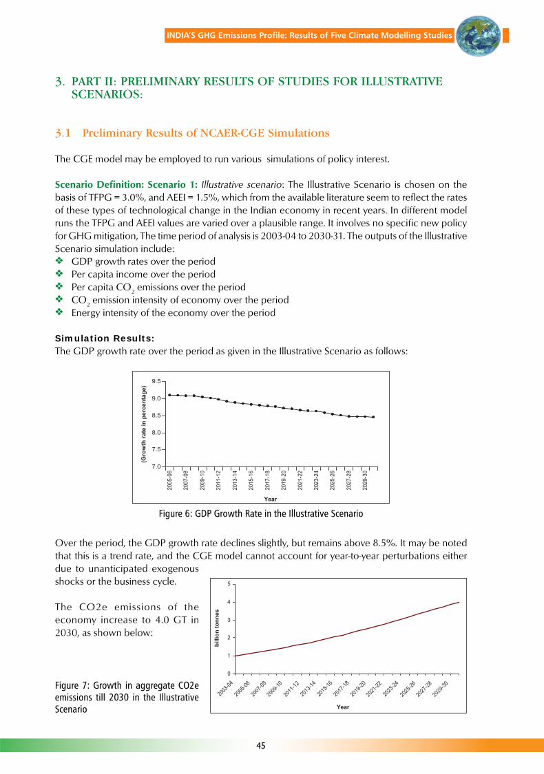
45


3. PART II: PRELIMINARY RESULTS OF STUDIES FOR ILLUSTRATIVESCENARIOS:

3.1 Preliminary Results of NCAER-CGE Simulations

The CGE model may be employed to run various simulations of policy interest.

Scenario Definition: Scenario 1: Illustrative scenario: The Illustrative Scenario is chosen on thebasis of TFPG = 3.0%, and AEEI = 1.5%, which from the available literature seem to reflect the ratesof these types of technological change in the Indian economy in recent years. In different modelruns the TFPG and AEEI values are varied over a plausible range. It involves no specific new policyfor GHG mitigation, The time period of analysis is 2003-04 to 2030-31. The outputs of the IllustrativeScenario simulation include:� GDP growth rates over the period� Per capita income over the period� Per capita CO2 emissions over the period� CO2 emission intensity of economy over the period� Energy intensity of the economy over the period

Simulation Results:The GDP growth rate over the period as given in the Illustrative Scenario as follows:

Figure 6: GDP Growth Rate in the Illustrative Scenario

Over the period, the GDP growth rate declines slightly, but remains above 8.5%. It may be notedthat this is a trend rate, and the CGE model cannot account for year-to-year perturbations eitherdue to unanticipated exogenousshocks or the business cycle.

The CO2e emissions of theeconomy increase to 4.0 GT in2030, as shown below:

Figure 7: Growth in aggregate CO2eemissions till 2030 in the IllustrativeScenario

46


The growth in per-capita CO2e emissions under the Illustrative Scenario was also provided by themodel, and is 2.77 tons CO2e per capita in 2030, as given below:

Figure 8: Growth in Per-Capita CO2e Emissions in the Illustrative Scenario

There is continuous decline in the energy intensity of the GDP, at a CAGR of -3.85 percent during2003-04 to 2030-31:

Figure 9: Change in energy intensity of the GDP during 2003-2030 in Illustrative Scenario

There is also continuous change in the CO2e intensity of the economy under the Illustrative Scenario,from 0.37 Kg CO2e in 2003 to 0.15 Kg CO2e in 2030, as shown below:

Figure 10: Change in CO2e Intensity of the GDP in the Illustrative Scenario

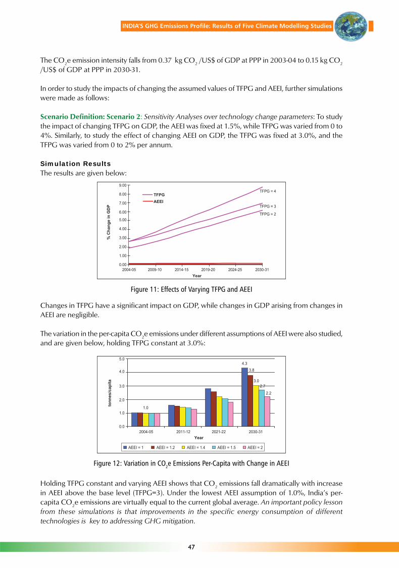
47


The CO2e emission intensity falls from 0.37 kg CO2 /US$ of GDP at PPP in 2003-04 to 0.15 kg CO2

/US$ of GDP at PPP in 2030-31.

In order to study the impacts of changing the assumed values of TFPG and AEEI, further simulationswere made as follows:

Scenario Definition: Scenario 2: Sensitivity Analyses over technology change parameters: To studythe impact of changing TFPG on GDP, the AEEI was fixed at 1.5%, while TFPG was varied from 0 to4%. Similarly, to study the effect of changing AEEI on GDP, the TFPG was fixed at 3.0%, and theTFPG was varied from 0 to 2% per annum.

Simulation ResultsThe results are given below:

Figure 11: Effects of Varying TFPG and AEEI

Changes in TFPG have a significant impact on GDP, while changes in GDP arising from changes inAEEI are negligible.

The variation in the per-capita CO2e emissions under different assumptions of AEEI were also studied,and are given below, holding TFPG constant at 3.0%:

Figure 12: Variation in CO2e Emissions Per-Capita with Change in AEEI

Holding TFPG constant and varying AEEI shows that CO2 emissions fall dramatically with increasein AEEI above the base level (TFPG=3). Under the lowest AEEI assumption of 1.0%, India’s per-capita CO2e emissions are virtually equal to the current global average. An important policy lessonfrom these simulations is that improvements in the specific energy consumption of differenttechnologies is key to addressing GHG mitigation.

48


3.2 Preliminary Results of TERI-MoEF Simulations

3.2.1 Scenario Definition:Simulations of the MARKAL model were carried out for the Illustrative scenario, i.e. with no newGHG abatement policies, TFPG=3.0, and specific energy consumption improvement consistentwith AEEI = 1.5, subject to feasibility limits of specific energy consumption for each technology.

Simulation Results: CO2 emissions from energy sources in the Illustrative scenario are estimated ataround 4.9 billion tonnes in 2031 (Figure 13):

Figure 13: CO2 emissions in the Illustrative Scenario

This is equivalent to 3.4 tonnes per capita CO2 emission in 2031 (Figure 14).

Figure 14: Trajectory of Per-capita CO2 emissions till 2031 in Illustrative Scenario

Figure 15 shows the commercial energy requirements over the 30-year modeling time frame for theIllustrative Scenario. The totalcommercial energy requirement in203‘1 is 1567 mtoe, and coalremains the dominant primaryenergy source.

Figure 15: Commercial energy supplyacross scenarios

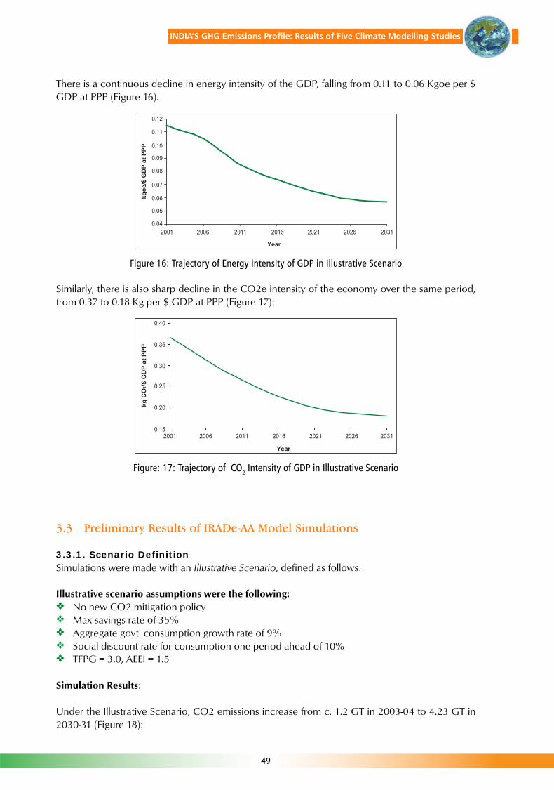
49


There is a continuous decline in energy intensity of the GDP, falling from 0.11 to 0.06 Kgoe per $GDP at PPP (Figure 16).

Figure 16: Trajectory of Energy Intensity of GDP in Illustrative Scenario

Similarly, there is also sharp decline in the CO2e intensity of the economy over the same period,from 0.37 to 0.18 Kg per $ GDP at PPP (Figure 17):

Figure: 17: Trajectory of CO2 Intensity of GDP in Illustrative Scenario

3.3 Preliminary Results of IRADe-AA Model Simulations

3.3.1. Scenario DefinitionSimulations were made with an Illustrative Scenario, defined as follows:

Illustrative scenario assumptions were the following:� No new CO2 mitigation policy� Max savings rate of 35%� Aggregate govt. consumption growth rate of 9%� Social discount rate for consumption one period ahead of 10%� TFPG = 3.0, AEEI = 1.5

Simulation Results:

Under the Illustrative Scenario, CO2 emissions increase from c. 1.2 GT in 2003-04 to 4.23 GT in2030-31 (Figure 18):

50


Figure 18: CO2 emissions in Illustrative Scenario

Year

4.50

4.00

3.50

3.00

2.50

2.00

1.50

1.000.50

0.002003 2006 2009 2012 2015 2018 2021 2024 2027

Illustrative scenario

2030

CO

2 em

issi

ons

(GT)

CO2 emissions under illustrative scenario

During this period, per capita CO2 emissions rise from about 1.1 tons per capita to under 2.9tonnes per capita. This is well below the 2005 global per-capita emissions of 4.22 tons per capita,(Figure 19):

Figure 19: Trajectory of Per-capita CO2e Emissions during 2001 to 2031 in Illustrative Scenario

There is also continuous decline in energy intensity in the Illustrative Scenario, from just over 0.1kgoe per $ GDP in PPP to c.0.04 kgoe per $ GDP in PPP.

Figure 20: Energy Intensity in Illustrative Scenario

There is a similar decline in the CO2 intensity of the economy in the Illustrative Scenario, fromabout 0.37 million tons CO2 per billion $ GDP in PPP to less than one-half, i.e. 0.15 million tonsCO2 per billion $ GDP at PPP.

51


Figure 21: CO2 Intensity under Illustrative Scenario

3.3.4: Results of TERI-Poznan (MARKAL) Study:Scenario Definition: The TERI-Poznan study defines the Illustrative Scenario as comprising efficiencyimprovements as per past trend and expert opinion considering level of maturity of specifictechnologies in India. The discount rate is assumed at 10% per annum, and the model considerseconomic costs. There is no new policy which bears on GHG mitigation.

Simulation Results: Under the Illustrative Scenario, GHG emissions increase to 7.3 billion tons in2031. This is shown in Figure 22 below:

Figure 22: CO2 emission in Illustrative scenario (2001-2031)

Figure 23: Per capita CO2 emission in Illustrative scenario

This works out to 5.0 tons per capita CO2 in 2031, Figure 23:

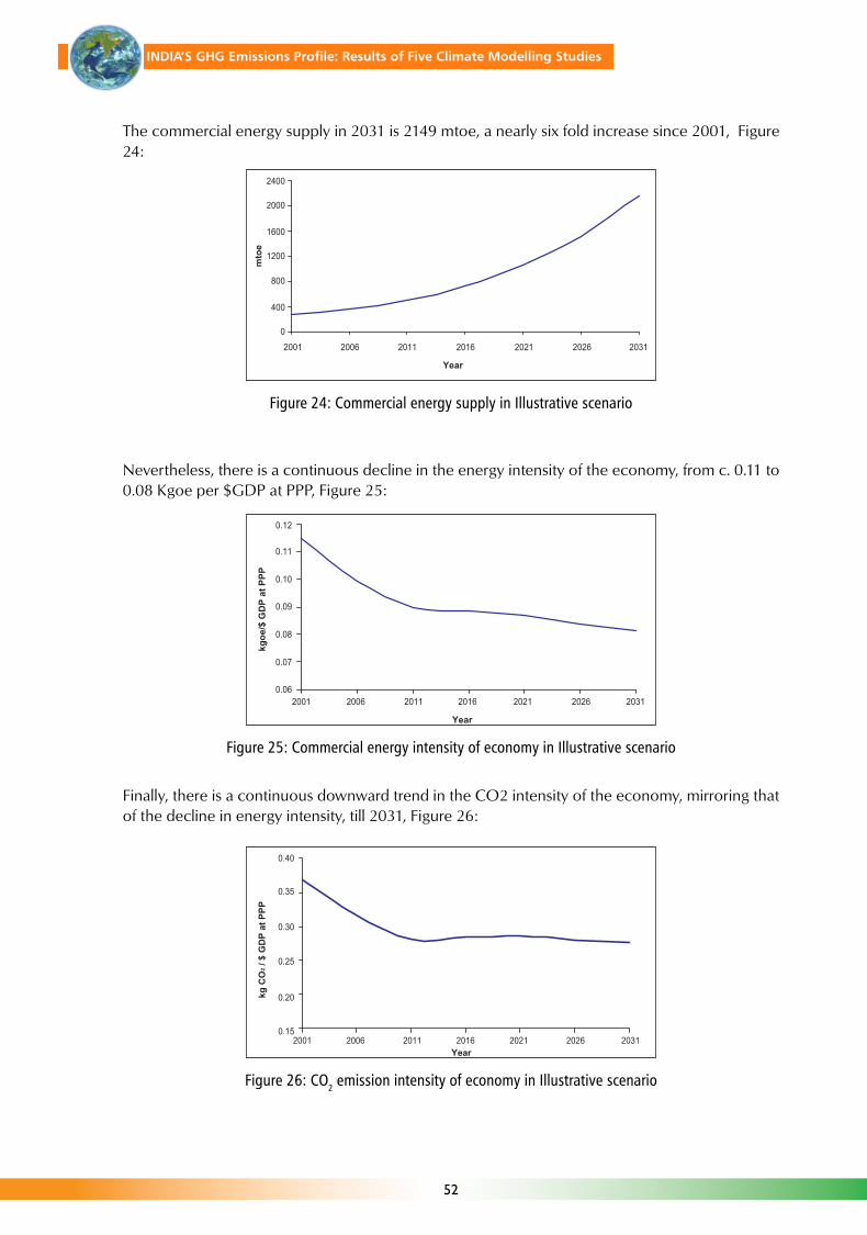
52


The commercial energy supply in 2031 is 2149 mtoe, a nearly six fold increase since 2001, Figure24:

Figure 24: Commercial energy supply in Illustrative scenario

Nevertheless, there is a continuous decline in the energy intensity of the economy, from c. 0.11 to0.08 Kgoe per $GDP at PPP, Figure 25:

Figure 25: Commercial energy intensity of economy in Illustrative scenario

Finally, there is a continuous downward trend in the CO2 intensity of the economy, mirroring thatof the decline in energy intensity, till 2031, Figure 26:

Figure 26: CO2 emission intensity of economy in Illustrative scenario

53


3.3.5: Results of McKinsey Bottom-up Study:The McKinsey Study makes the following assumptions with respect to the Illustrative Scenario:

Scenario Definition: The Illustrative Scenario is defined by the following assumptions:

Parameter Illustrative Scenario assumption

Total energy demand 1.7 billion toePower demand 3870 TWh (including captive)Base and non-base power demand 60:40Power capacity mix (including captive In GW 2005 2030and spinning reserves) Total 150 760

Share of clean andrenewable power2 25% 29%

Area under forests / degraded area by 2030 86 Mha/15 MhaTechnical T&D losses and auxiliary consumption 12% and 6%

2 Includes nuclear, solar, hydro, biomass, geothermal and wind power

Study Results:

The trajectory of aggregate GHG emission in the Illustrative Scenario till the year 2030-31 is presentedbelow:

GHG emissions in year (GtCO2e) 2005 2020 2030

Illustrative Scenario 1.6 3.2 5.7

Note: All emissions in billion tonnes CO2e. Emissions include CO2, CH4 and N2O weighted by theirrespective GWPs.

The aggregate GHG emissions increase from 1.6 GT in 2005 to 5.7 GT in 2030. This works out to3.9 tons/CO2e per capita in 2030.

The changes in energy intensity and GHG intensity of the economy in the Illustrative Scenario from2005 to 2030 are given below:

Model output Illustrative Scenario

Change in energy intensity (CAGR) 2005-2030; implied -2.6% p.a.Change in GHG intensity (CAGR) 2005-2030; implied -2.1% p.a.

There is a continuous decline in both energy intensity of the GDP, as well as of the GHG intensity ofthe economy, at CAGRs of -2.6% and [email protected]% per annum respectively.

54


3.4 Conclusions:

The results of 4 of the 5 studies, which vary in terms of model structure/methodology, assumptions,and data, besides differences in the definitions of the Illustrative Scenario, whose common featureis that no new GHG mitigation policies are put in place, show that India’s per-capita CO2e emissionsin 2030/31 would be between 2.77 and 3.9 tons per-capita, which is well below the 2005 globalaverage of 4.22 tons per-capita. The fifth study projects the 2031 emissions at 5 tons per-capita, i.e.a little above the 2005 global average.

Further, both the energy intensity of the Indian economy, as well as the CO2e intensity of the Indianeconomy fall continuously till 2030-31 in the Illustrative Scenarios, as revealed by all 5 studies.

The results should set at rest any apprehensions that India’s GHG emissions are poised for runawayincrease over the next two decades. On the other hand, the structure of the economy, policy andregulatory regime, and energy endowments, together ensure that India’s growth over the next twodecades, while rapid, would remain inherently sustainable.

The fact that significant differences still arise between the results of the different studies show thatit is not feasible to unambiguously define any “baseline” or “business-as-usual” GHGs trajectory forthe country.

Thus, even without any new policies for GHG abatement and given the structure of the Indianeconomy, its current and projected GHG growth rates, and its energy endowments, there can beno apprehension that its GHG emissions will increase in a runaway manner over time. India’s energyuse patterns and GHG emissions profile will continue to be among the most sustainable in theworld for the next generation.

55


Babiker, M.H., J.M. Reilly, M. Mayer, R.S. Eckaus, I.S. Wing and R.C. Hyman (2001), ‘The MIT EmissionsPrediction and Policy Analysis (EPPA) Model: Revisions, Sensitivities and Comparison of Results’,Report no. 71, MIT Joint Program on the Science and Policy of Global Change. Cambridge, M.A.

Burniaux, J.M., G. Nicoletti, and J.O. Martins (1992), ‘GREEN: A Global Model for Quantifying theCost of Policies to Curb CO2 Emissions’, OECD Economic Studies, no.19. Paris.

Ghosh, Prodipto (1990).“Simulating Greenhouse Gases Emissions due to Energy Use by a ComputableGeneral equilibrium Model of a National Economy”: Ph.D dissertation research, Carnegie-MellonUniversity. Published by UMI, Ann Arbor, MI. Order No. DA9107559.

Robinson, Sherman et al (1999), ‘From Stylized to Applied Models : Building Multisector CGE Modelsfor Policy Analysis’, North American Journal of Economics and Finance, vol. 10, no.2, 5-38.

TERI (2006), National energy Map for India: Technology Vision 2030. The Energy and ResourcesInstitute (TERI), New Delhi.

References:

56


1. NCAER-CGE:

Vijay P OjhaSanjib PohitBarun Deb Pal

2. TERI-MoEF:

Ritu MathurAtul KumarAmrita GoldarIla GuptaNishant Mehra

3. IRADe-AA:

Jyoti ParikhProbal Ghosh

Technical Coordinator for above models: Prodipto Ghosh

4. TERI-Poznan:

Leena SrivastavaRitu MathurAtul KumarAmrita GoldarIla GuptaNishant MehraPradeep K. Dadhich

5. McKinsey Study:

Rajat GuptaSahana SarmaRahul SankheSushant Mantry

Team Members of the Studies:

CONTACT US

CLIMATE CHANGE DIVISIONMinistry of Environment & ForestsGovernment of IndiaParyavaran BhawanCGO Complex, Lodi RoadNew Delhi – 110 003Tel: 24932281 / 24362252Tel/Fax: 243607681 / 24362252E-mail: [email protected]

[email protected]@nic.in

Web: www.envfor.nic.in

‘india’s ghg emissions profile: results of five climate modelling studies’

Documents

indias ghg emissions

greenhouse gas ghg emissions

thatthese studies

climatemodelling studies

independentmodelling

indias ghgemissions

climate change ipcc

research work