This is a preprint of an article accepted for publication inEarthquake Engng Struct. Dyn.Copyright c©2002 John Wiley & Sons, Ltd.

Incremental Dynamic Analysis

Dimitrios Vamvatsikos† and C.Allin Cornell‡,∗

Department of Civil and Environmental Engineering, Stanford University, CA 94305-4020, U.S.A.

SUMMARY

Incremental Dynamic Analysis (IDA) is a parametric analysis method that has recently emerged in severaldifferent forms to estimate more thoroughly structural performance under seismic loads. It involves subjectinga structural model to one (or more) ground motion record(s), each scaled to multiple levels of intensity, thusproducing one (or more) curve(s) of response parameterized versus intensity level. To establish a common frameof reference, the fundamental concepts are analyzed, a unified terminology is proposed, suitable algorithms arepresented, and properties of the IDA curve are looked into for both single-degree-of-freedom (SDOF) and multi-degree-of-freedom (MDOF) structures. In addition, summarization techniques for multi-record IDA studies andthe association of the IDA study with the conventional Static Pushover Analysis and the yield reductionR-factorare discussed. Finally in the framework of Performance-Based Earthquake Engineering (PBEE), the assessmentof demand and capacity is viewed through the lens of an IDA study.

KEY WORDS: performance-based earthquake engineering; incremental dynamic analysis; demand; collapsecapacity; limit-state; nonlinear dynamic analysis

1 INTRODUCTION

The growth in computer processing power has made possible a continuous drive towards increasinglyaccurate but at the same time more complex analysis methods. Thus the state of the art has pro-gressively moved from elastic static analysis to dynamic elastic, nonlinear static and finally nonlineardynamic analysis. In the last case the convention has been to run one to several different records,each once, producing one to several “single-point” analyses, mostly used for checking the designedstructure. On the other hand methods like the nonlinear static pushover (SPO) [1] or the capacityspectrum method [1] offer, by suitable scaling of the static force pattern, a “continuous” picture as thecomplete range of structural behavior is investigated, from elasticity to yielding and finally collapse,thus greatly facilitating our understanding.

By analogy with passing from a single static analysis to the incremental static pushover, one arrivesat the extension of a single time-history analysis into an incremental one, where the seismic “loading”is scaled. The concept has been mentioned as early as 1977 by Bertero [2], and has been cast in severalforms in the work of many researchers, including Luco and Cornell [3, 4], Bazurro and Cornell [5, 6],Yun and Foutch [7], Mehanny and Deierlein [8], Dubinaet al. [9], De Matteiset al. [10], Nassar and

†Graduate Student‡Professor∗Correspondence to: C.Allin Cornell, Department of Civil and Environmental Engineering, Stanford University, Stan-

ford, CA 94305-4020, U.S.A. email: cornell@ce.stanford.edu

1

0 0.05 0.1 0.15 0.2 0.250

0.05

0.1

0.15

0.2

0.25

maximum interstory drift ratio, θ max

"firs

t−m

ode"

spe

ctra

l acc

eler

atio

n S

a(T

1, 5

%)

(g)

(a) Single IDA curve versus Static Pushover

Sa = 0.2g

Sa = 0.1g

Sa = 0.01g

Static Pushover Curve

IDA curve

0 0.01 0.02 0.03 0.04 0.05 0.060

2

4

6

8

10

12

14

16

18

20 (b) Peak interstorey drift ratio versus storey level

peak interstorey drift ratio θi

stor

ey le

vel

Sa = 0.01g

Sa = 0.2g

Sa = 0.1g

Figure 1.An example of information extracted from a single-record IDA study of aT1 = 4 sec, 20-storey steelmoment-resisting frame with ductile members and connections, including global geometric nonlinearities (P–∆)

subjected to the El Centro, 1940 record (fault parallel component).

2

Krawinkler [11, pg.62–155] and Psychariset al. [12]. Recently, it has also been adopted by the U.S.Federal Emergency Management Agency (FEMA) guidelines [13, 14] as the Incremental DynamicAnalysis (IDA) and established as the state-of-the-art method to determine global collapse capacity.The IDA study is now a multi-purpose and widely applicable method and its objectives, only some ofwhich are evident in Figure1(a,b), include

1. thorough understanding of the range of response or “demands” versus the range of potentiallevels of a ground motion record,

2. better understanding of the structural implications of rarer / more severe ground motion levels,

3. better understanding of the changes in the nature of the structural response as the intensityof ground motion increases (e.g., changes in peak deformation patterns with height, onset ofstiffness and strength degradation and their patterns and magnitudes),

4. producing estimates of the dynamic capacity of the global structural system and

5. finally, given a multi-record IDA study, how stable (or variable) all these items are from oneground motion record to another.

Our goal is to provide a basis and terminology to unify the existing formats of the IDA study andset up the essential background to achieve the above-mentioned objectives.

2 FUNDAMENTALS OF SINGLE-RECORD IDAS

As a first step, let us clearly define all the terms that we need, and start building our methodologyusing as a fundamental block the concept of scaling an acceleration time history.

Assume we are given a single acceleration time-history, selected from a ground motion database,which will be referred to as the base, “as-recorded” (although it may have been pre-processed byseismologists, e.g., baseline corrected, filtered and rotated), unscaled accelerograma1, a vector withelementsa1(ti), ti = 0, t1, . . . , tn−1. To account for more severe or milder ground motions, a simpletransformation is introduced by uniformly scaling up or down the amplitudes by a scalarλ ∈ [0,+∞):aλ = λ · a1. Such an operation can also be conveniently thought of as scaling the elastic accelera-tion spectrum byλ or equivalently, in the Fourier domain, as scaling byλ the amplitudes across allfrequencies while keeping phase information intact.

Definition 1. The SCALE FACTOR (SF) of a scaled accelerogram,aλ , is the non-negative scalarλ ∈ [0,+∞) that producesaλ when multiplicatively applied to the unscaled (natural) accelerationtime-historya1.

Note how theSF constitutes a one-to-one mapping from the original accelerogram to all its scaledimages. A value ofλ = 1 signifies the natural accelerogram,λ < 1 is a scaled-down accelerogram,while λ > 1 corresponds to a scaled-up one.

Although theSF is the simplest way to characterize the scaled images of an accelerogram it isby no means convenient for engineering purposes as it offers no information of the real “power” ofthe scaled record and its effect on a given structure. Of more practical use would be a measure thatwould map to theSF one-to-one, yet would be more informative, in the sense of better relating to itsdamaging potential.

3

Definition 2. A MONOTONIC SCALABLE GROUND MOTION INTENSITY MEASURE (or simply in-tensity measure,IM ) of a scaled accelerogram,aλ , is a non-negative scalarIM ∈ [0,+∞) that consti-tutes a function,IM = fa1(λ ), that depends on the unscaled accelerogram,a1, and is monotonicallyincreasing with the scale factor,λ .

While many quantities have been proposed to characterize the “intensity” of a ground motionrecord, it may not always be apparent how to scale them, e.g., Moment Magnitude, Duration, or Mod-ified Mercalli Intensity; they must be designated as non-scalable. Common examples of scalableIM sare the Peak Ground Acceleration (PGA), Peak Ground Velocity, theξ = 5% damped Spectral Ac-celeration at the structure’s first-mode period (Sa(T1,5%)), and the normalized factorR = λ/λyield

(whereλyield signifies, for a given record and structural model, the lowest scaling needed to causeyielding) which is numerically equivalent to the yield reductionR-factor (e.g., [15]) for, for exam-ple, bilinear SDOF systems (see later section). TheseIM s also have the property of being pro-portional to theSF as they satisfy the relationIMprop = λ · fa1. On the other hand the quantitySam(T1,ξ ,b,c,d) = [Sa(T1,ξ )]b · [Sa(cT1,ξ )]d proposed by Shome and Cornell [16] and Mehanny [8]is scalable and monotonic but non-proportional, unlessb+ d = 1. Some non-monotonicIM s havebeen proposed, such as the inelastic displacement of a nonlinear oscillator by Luco and Cornell [17],but will not be focused upon, soIM will implicitly mean monotonic and scalable hereafter unlessotherwise stated.

Now that we have the desired input to subject a structure to, we also need some way to monitor itsstate, its response to the seismic load.

Definition 3. DAMAGE MEASURE (DM) or STRUCTURAL STATE VARIABLE is a non-negativescalarDM ∈ [0,+∞] that characterizes the additional response of the structural model due to a pre-scribed seismic loading.

In other words aDM is an observable quantity that is part of, or can be deduced from, the outputof the corresponding nonlinear dynamic analysis. Possible choices could be maximum base shear,node rotations, peak storey ductilities, various proposed damage indices (e.g., a global cumulativehysteretic energy, a global Park–Ang index [18] or the stability index proposed by Mehanny [8]), peakroof drift, the floor peak interstorey drift anglesθ1, . . . ,θn of ann-storey structure, or their maximum,the maximum peak interstorey drift angleθmax = max(θ1, . . . ,θn). Selecting a suitableDM dependson the application and the structure itself; it may be desirable to use two or moreDM s (all resultingfrom the same nonlinear analyses) to assess different response characteristics, limit-states or modesof failure of interest in a PBEE assessment. If the damage to non-structural contents in a multi-storeyframe needs to be assessed, the peak floor accelerations are the obvious choice. On the other hand,for structural damage of frame buildings,θmax relates well to joint rotations and both global and localstorey collapse, thus becoming a strongDM candidate. The latter, expressed in terms of the total drift,instead of the effective drift which would take into account the building tilt, (see [19, pg.88]) will beour choice ofDM for most illustrative cases here, where foundation rotation and column shorteningare not severe.

The structural response is often a signed scalar; usually, either the absolute value is used or themagnitudes of the negative and the positive parts are separately considered. Now we are able to definethe IDA.

Definition 4. A SINGLE-RECORD IDA STUDY is a dynamic analysis study of a given structuralmodel parameterized by the scale factor of the given ground motion time history.

4

Also known simply as Incremental Dynamic Analysis (IDA) or Dynamic Pushover (DPO), it in-volves a series of dynamic nonlinear runs performed under scaled images of an accelerogram, whoseIM s are, ideally, selected to cover the whole range from elastic to nonlinear and finally to collapse ofthe structure. The purpose is to recordDM s of the structural model at each levelIM of the scaledground motion, the resulting response values often being plotted versus the intensity level as continu-ous curves.

Definition 5. An IDA CURVE is a plot of a state variable (DM) recorded in an IDA study versus oneor moreIMs that characterize the applied scaled accelerogram.

An IDA curve can be realized in two or more dimensions depending on the number of theIM s.Obviously at least one must be scalable and it is such anIM that is used in the conventional two-dimensional (2D) plots that we will focus on hereafter. As per standard engineering practice suchplots often appear “upside-down” as the independent variable is theIM which is considered analogousto “force” and plotted on the vertical axis (Figure1(a)) as in stress-strain, force-deformation or SPOgraphs. As is evident, the results of an IDA study can be presented in a multitude of different IDAcurves, depending on the choices ofIM s andDM .

To illustrate the IDA concept we will use several MDOF and SDOF models as examples in thefollowing sections. In particular the MDOFs used are aT1 = 4 sec 20-storey steel-moment resistingframe [3] with ductile members and connections, including a first-order treatment of global geometricnonlinearities (P–∆ effects), aT1 = 2.2 sec 9-storey and aT1 = 1.3 sec 3-storey steel-moment resistingframe [3] with ductile members, fracturing connections and P–∆ effects, and aT1 = 1.8 sec 5-storeysteel chevron-braced frame with ductile members and connections and realistically buckling bracesincluding P–∆ effects [6].

3 LOOKING AT AN IDA CURVE: SOME GENERAL PROPERTIES

The IDA study isaccelerogramandstructural modelspecific; when subjected to different ground mo-tions a model will often produce quite dissimilar responses that are difficult to predict a priori. Notice,for example, Figure2(a–d) where a 5-storey braced frame exhibits responses ranging from a grad-ual degradation towards collapse to a rapid, non-monotonic, back-and-forth twisting behavior. Eachgraph illustrates thedemandsimposed upon the structure by each ground motion record at differentintensities, and they are quite intriguing in both their similarities and dissimilarities.

All curves exhibit a distinct elastic linear region that ends atSyielda (T1,5%) ≈ 0.2g andθ yield

max ≈0.2%when the first brace-buckling occurs. Actually, any structural model with initially linearly elasticelements will display such a behavior, which terminates when the first nonlinearity comes into play,i.e., when any element reaches the end of its elasticity. The slopeIM/DM of this segment on eachIDA curve will be called its elastic “stiffness” for the givenDM , IM . It typically varies to some degreefrom record to record but it will be the same across records for SDOF systems and even for MDOFsystems if theIM takes into account the higher mode effects (i.e., Luco and Cornell [17]).

Focusing on the other end of the curves in Figure2, notice how they terminate at different levels ofIM . Curve (a) sharply “softens” after the initial buckling and accelerates towards large drifts and even-tual collapse. On the other hand, curves (c) and (d) seem to weave around the elastic slope; they followclosely the familiarequal displacementrule, i.e., the empirical observation that for moderate periodstructures, inelastic global displacements are generally approximately equal to the displacements ofthe corresponding elastic model (e.g., [20]). The twisting patterns that curves (c) and (d) display indoing so are successive segments of “softening” and “hardening”, regions where the local slope or

5

0 0.01 0.02 0.030

0.5

1

1.5

(a) A softening case

0 0.01 0.02 0.030

0.5

1

1.5

(b) A bit of hardening

0 0.01 0.02 0.030

0.5

1

1.5

(c) Severe hardening

maximum interstory drift ratio, θ max

"firs

t−m

ode"

spe

ctra

l acc

eler

atio

n S

a(T1, 5

%)

(g)

0 0.01 0.02 0.030

0.5

1

1.5

(d) Weaving behavior

Figure 2.IDA curves of aT1 = 1.8 sec, 5-storey steel braced frame subjected to 4 different records.

“stiffness” decreases with higherIM and others where it increases. In engineering terms this meansthat at times the structure experiences acceleration of the rate ofDM accumulation and at other timesa deceleration occurs that can be powerful enough to momentarily stop theDM accumulation or evenreverse it, thus locally pulling the IDA curve to relatively lowerDM s and making it a non-monotonicfunction of theIM (Figure2(d)). Eventually, assuming the model allows for some collapse mechanismand theDM used can track it, a final softening segment occurs when the structure accumulatesDMat increasingly higher rates, signaling the onset ofdynamic instability. This is defined analogouslyto static instability, as the point where deformations increase in an unlimited manner for vanishinglysmall increments in theIM . The curve then flattens out in a plateau of the maximum value inIM as itreaches theflatline andDM moves towards “infinity” (Figure2(a,b)). Although the examples shownare based onSa(T1,5%) andθmax, these modes of behavior are observable for a wide choice ofDM sandIM s.

Hardening in IDA curves is not a novel observation, having been reported before even for simplebilinear elastic-perfectly-plastic systems, e.g., by Chopra [15, pg.257-259]. Still it remains counter-intuitive that a system that showed high response at a given intensity level, may exhibit the same oreven lower response when subjected to higher seismic intensities due to excessive hardening. But it isthepatternand thetiming rather than just the intensity that make the difference. As the accelerogramis scaled up, weak response cycles in the early part of the response time-history become strong enoughto inflict damage (yielding) thus altering the properties of the structure for the subsequent, strongercycles. For multi-storey buildings, a stronger ground motion may lead to earlier yielding of one floorwhich in turn acts as a fuse to relieve another (usually higher) one, as in Figure3. Even simpleoscillators when caused to yield in an earlier cycle, may be proven less responsive in later cycles that

6

0 0.005 0.01 0.015 0.02 0.025 0.03

0.2

0.4

0.6

0.8

1

1.2

1.4

storey 1 storey 2 storey 3

storey 4

storey 5

maximum interstory drift ratio, θ max

"firs

t−m

ode"

spe

ctra

l acc

eler

atio

n S

a(T

1, 5

%)

(g)

Figure 3.IDA curves of peak interstorey drifts for each floor of aT1 = 1.8 sec 5-storey steel braced frame.Notice the complex “weaving” interaction where extreme softening of floor 2 acts as a fuse to relieve those

above (3,4,5).

had previously caused higherDM values (Figure4), perhaps due to “period elongation”. The samephenomena account for thestructural resurrection, an extreme case of hardening, where a system ispushed all the way to global collapse (i.e., the analysis code cannot converge, producing “numericallyinfinite” DM s) at someIM , only to reappear as non-collapsing at a higher intensity level, displayinghigh response but still standing (e.g., Figure5).

As the complexity of even the 2D IDA curve becomes apparent, it is only natural to examine theproperties of the curve as a mathematical entity. Assuming a monotonicIM the IDA curve becomes afunction([0,+∞)→ [0,+∞]), i.e., any value ofIM produces a single valueDM , while for any givenDM value there is at least one or more (in non-monotonic IDA curves)IM s that generate it, since themapping is not necessarily one-to-one. Also, the IDA curve is not necessarily smooth as theDM isoften defined as a maximum or contains absolute values of responses, making it non-differentiable bydefinition. Even more, it may contain a (hopefully finite) number of discontinuities, due to multipleexcursions to collapse and subsequent resurrections.

4 CAPACITY AND LIMIT-STATES ON SINGLE IDA CURVES

Performance levels or limit-states are important ingredients of Performance Based Earthquake Engi-neering (PBEE), and the IDA curve contains the necessary information to assess them. But we needto define them in a less abstract way that makes sense on an IDA curve, i.e., by a statement or arule

7

0 0.5 1 1.5 2 2.5 3 3.5 40

0.5

1

1.5

2

2.5

3

3.5

"firs

t−m

ode"

spe

ctra

l acc

eler

atio

n S

a(T1, 5

%)

(g)

(a) IDA curve

Sa = 2.8g

ductility, µ

Sa = 2.2g

0 5 10 15 20 25 30 35 40

−0.1

−0.05

0

0.05

0.1

Acc

eler

atio

n (g

)

(b) Loma Prieta, Halls Valley (090 component)

0 5 10 15 20 25 30 35 40

−2

0

2

(c) Response at Sa = 2.2g

duct

ility

, µ

0 5 10 15 20 25 30 35 40

−2

0

2

(d) Response at Sa = 2.8g

duct

ility

, µ

time (sec)

maximum

maximum

first yield

first yield

Figure 4.Ductility response of aT = 1 sec, elasto-plastic oscillator at multiple levels of shaking. Earlieryielding in the stronger ground motion leads to a lower absolute peak response.

8

0 0.05 0.1 0.150

0.2

0.4

0.6

0.8

1

1.2

1.4

1.6

1.8

maximum interstory drift ratio, θ max

"firs

t−m

ode"

spe

ctra

l acc

eler

atio

n S

a(T1, 5

%)

(g)

structural resurrection

intermediate collapse area

Figure 5.Structural resurrection on the IDA curve of aT1 = 1.3 sec, 3-storey steel moment-resisting frame withfracturing connections.

that when satisfied, signals reaching a limit-state. For example, Immediate Occupancy [13, 14] is astructural performance level that has been associated with reaching a givenDM value, usually inθmax

terms, while (in FEMA 350 [13], at least) Global Collapse is related to theIM or DM value wheredynamic instability is observed. A relevant issue that then appears is what to do when multiple points(Figure6(a,b)) satisfy such a rule? Which one is to be selected?

The cause of multiple points that can satisfy a limit-state rule is mainly the hardening issue and, inits extreme form, structural resurrection. In general, one would want to be conservative and considerthe lowest, inIM terms, point that will signal the limit-state. Generalizing this concept to the wholeIDA curve means that we will discard its portion “above” the first (inIM terms) flatline and justconsider only points up to this first sign of dynamic instability.

Note also that for most of the discussion we will be equating dynamic instability to numericalinstability in the prediction of collapse. Clearly the non-convergence of the time-integration schemeis perhaps the safest and maybe the only numerical equivalent of the actual phenomenon of dynamiccollapse. But, as in all models, this one can suffer from the quality of the numerical code, the steppingof the integration and even the round-off error. Therefore, we will assume that such matters are takencare of as well as possible to allow for accurate enough predictions. That being said, let us set forththe most basic rules used to define a limit-state.

First comes theDM-based rule, which is generated from a statement of the format: “IfDM ≥CDM then the limit-state is exceeded” (Figure6(a)). The underlying concept is usually thatDM is adamage indicator, hence, when it increases beyond a certain value the structural model is assumed tobe in the limit-state. Such values ofCDM can be obtained through experiments, theory or engineering

9

0 0.05 0.1 0.15 0.2 0.250

0.2

0.4

0.6

0.8

1

1.2

1.4

1.6

1.8

maximum interstory drift ratio, θ max

"firs

t−m

ode"

spe

ctra

l acc

eler

atio

n S

a(T1, 5

%)

(g)

(a) DM−based rule

collapse

CDM

= 0.08

capacity point

0 0.05 0.1 0.15 0.2 0.250

0.2

0.4

0.6

0.8

1

1.2

1.4

1.6

1.8

maximum interstory drift ratio, θ max

"firs

t−m

ode"

spe

ctra

l acc

eler

atio

n S

a(T1, 5

%)

(g)

(b) IM−based rule

collapse

CIM

= 1.61g capacity point

rejected point

Figure 6. Two different rules producing multiple capacity points for aT1 = 1.3 sec, 3-storey steel moment-resisting frame with fracturing connections. TheDM rule, where theDM is θmax, is set atCDM = 0.08 and the

IM rule uses the20%slope criterion.

10

experience, and they may not be deterministic but have a probability distribution. An example isthe θmax = 2% limit that signifies the Immediate Occupancy structural performance level for steelmoment-resisting frames (SMRFs) with type-1 connections in the FEMA guidelines [14]. Also theapproach used by Mehanny and Deierlein [8] is another case where a structure-specific damage indexis used asDM and when its reciprocal is greater than unity, collapse is presumed to have occurred.Such limits may have randomness incorporated, for example, FEMA 350 [13] defines a local collapselimit-state by the value ofθmax that induces a connection rotation sufficient to destroy the gravity loadcarrying capacity of the connection. This is defined as a random variable based on tests, analysis andjudgment for each connection type. Even a uniqueCDM value may imply multiple limit-state pointson an IDA curve (e.g., Figure6(a)). This ambiguity can be handled by an ad hoc, specified procedure(e.g., by conservatively defining the limit-state point as the lowestIM ), or by explicitly recognizing themultiple regions conforming and non-conforming with the performance level. TheDM -based ruleshave the advantage of simplicity and ease of implementation, especially for performance levels otherthan collapse. In the case of collapse capacity though, they may actually be a sign of model deficiency.If the model is realistic enough it ought to explicitly contain such information, i.e., show a collapse bynon-convergence instead of by a finiteDM output. Still, one has to recognize that such models canbe quite complicated and resource-intensive, while numerics can often be unstable. HenceDM -basedcollapse limit-state rules can be quite useful. They also have the advantage of being consistent withother less severe limit-states which are more naturally identified inDM terms, e.g.,θmax.

The alternativeIM-based rule, is primarily generated from the need to better assess collapse capac-ity, by having a single point on the IDA curve that clearly divides it to two regions, one of non-collapse(lower IM ) and one of collapse (higherIM ). For monotonicIM s, such a rule is generated by a state-ment of the form: “IfIM ≥CIM then the limit-state is exceeded” (Figure6(b)). A major differencewith the previous category is the difficulty in prescribing aCIM value that signals collapse for all IDAcurves, so it has to be done individually, curve by curve. Still, the advantage is that it clearly generatesa single collapse region, and the disadvantage is the difficulty of defining such a point for each curvein a consistent fashion. In general, such a rule results in bothIM andDM descriptions of capacity. Aspecial (extreme) case is taking the “final” point of the curve as the capacity, i.e., by using the (low-est) flatline to define capacity (inIM terms), where all of the IDA curve up to the first appearance ofdynamic instability is considered as non-collapse.

The FEMA [13] 20% tangent slope approach is, in effect, anIM -based rule; thelast point on thecurve with a tangent slope equal to 20% of the elastic slope is defined to be the capacity point. Theidea is that the flattening of the curve is an indicator of dynamic instability (i.e., theDM increasingat ever higher rates and accelerating towards “infinity”). Since “infinity” is not a possible numericalresult, we content ourselves with pulling back to a rate ofθmax increase equal to five times the initial orelastic rate, as the place where we mark the capacity point. Care needs to be exercised, as the possible“weaving” behavior of an IDA curve can provide several such points where the structure seems tohead towards collapse, only to recover at a somewhat higherIM level, as in Figure6(b); in principle,these lower points should thus be discarded as capacity candidates. Also the non-smoothness of theactual curve may prove to be a problem. As mentioned above, the IDA curve is at best piecewisesmooth, but even so, approximate tangent slopes can be assigned to every point along it by employinga smooth interpolation. For sceptics this may also be thought of as a discrete derivative on a grid ofpoints that is a good “engineering” approximation to the “rate-of-change”.

The above mentioned simple rules are the building blocks to construct composite rules, i.e., com-posite logical clauses of the above types, most often joined by logical OR operators. For example,when a structure has several collapse modes, not detectable by a singleDM , it is advantageous to

11

detect global collapse with an OR clause for each individual mode. An example is offshore platformswhere pile or soil failure modes are evident in deck drift while failures of braces are more evident inmaximum peak inter-tier drift. The first — inIM terms — event that occurs is the one that governscollapse capacity. Another case is Global Collapse capacity, which as defined by FEMA in [13, 14] isin fact an OR conjunction of the 20% slopeIM -based rule and aCDM = 10%DM -based rule, whereSa(T1,5%) andθmax are theIM andDM of choice. If either of the two rules obtains, it defines capac-ity. This means that the 20% stiffness detects impending collapse, while the 10% cap guards againstexcessive values ofθmax, indicative of regions where the model may not be trustworthy. As aDMdescription of capacity is proposed, this definition may suffer from inaccuracies, since close to theflatline a wide range ofDM values may correspond to only a small range ofIM s, thus making theactual value ofDM selected sensitive to the quality of IDA curve tracing and to the (ad hoc) 20%value. If, on the other hand, anIM description is used, the rule becomes more robust. This is a generalobservation for collapse capacity; it appears that it can be best expressed inIM terms.

5 MULTI-RECORD IDAS AND THEIR SUMMARY

As should be evident by now, a single-record IDA study cannot fully capture the behavior a buildingmay display in a future event. The IDA can be highly dependent on the record chosen, so a sufficientnumber of records will be needed to cover the full range of responses. Hence, we have to resort tosubjecting the structural model to a suite of ground motion records.

Definition 6. A MULTI -RECORD IDA STUDY is a collection of single-record IDA studies of the samestructural model, under different accelerograms.

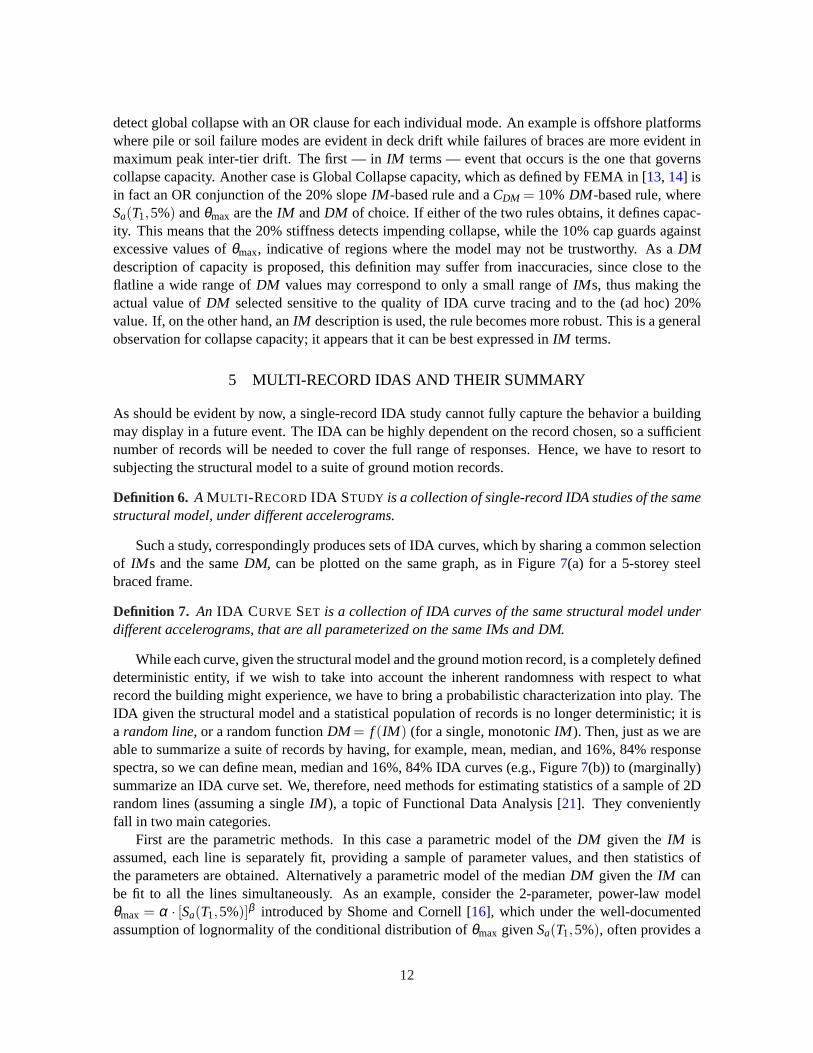
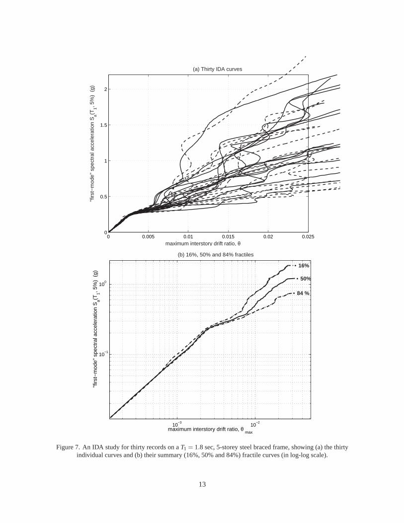
Such a study, correspondingly produces sets of IDA curves, which by sharing a common selectionof IM s and the sameDM, can be plotted on the same graph, as in Figure7(a) for a 5-storey steelbraced frame.

Definition 7. An IDA CURVE SET is a collection of IDA curves of the same structural model underdifferent accelerograms, that are all parameterized on the sameIMs andDM.

While each curve, given the structural model and the ground motion record, is a completely defineddeterministic entity, if we wish to take into account the inherent randomness with respect to whatrecord the building might experience, we have to bring a probabilistic characterization into play. TheIDA given the structural model and a statistical population of records is no longer deterministic; it isa random line, or a random functionDM = f (IM ) (for a single, monotonicIM ). Then, just as we areable to summarize a suite of records by having, for example, mean, median, and 16%, 84% responsespectra, so we can define mean, median and 16%, 84% IDA curves (e.g., Figure7(b)) to (marginally)summarize an IDA curve set. We, therefore, need methods for estimating statistics of a sample of 2Drandom lines (assuming a singleIM ), a topic of Functional Data Analysis [21]. They convenientlyfall in two main categories.

First are the parametric methods. In this case a parametric model of theDM given theIM isassumed, each line is separately fit, providing a sample of parameter values, and then statistics ofthe parameters are obtained. Alternatively a parametric model of the medianDM given theIM canbe fit to all the lines simultaneously. As an example, consider the 2-parameter, power-law modelθmax = α · [Sa(T1,5%)]β introduced by Shome and Cornell [16], which under the well-documentedassumption of lognormality of the conditional distribution ofθmax givenSa(T1,5%), often provides a

12

0 0.005 0.01 0.015 0.02 0.0250

0.5

1

1.5

2

maximum interstory drift ratio, θ max

"firs

t−m

ode"

spe

ctra

l acc

eler

atio

n S

a(T1, 5

%)

(g)

(a) Thirty IDA curves

10−3

10−2

10−1

100

maximum interstory drift ratio, θ max

"firs

t−m

ode"

spe

ctra

l acc

eler

atio

n S

a(T1, 5

%)

(g)

• 50%

• 16%

• 84 %

(b) 16%, 50% and 84% fractiles

Figure 7.An IDA study for thirty records on aT1 = 1.8 sec, 5-storey steel braced frame, showing (a) the thirtyindividual curves and (b) their summary (16%, 50% and 84%) fractile curves (in log-log scale).

13

simple yet powerful description of the curves, allowing some important analytic results to be obtained[22, 23]. This is a general property of parametric methods; while they lack the flexibility to accuratelycapture each curve, they make up by allowing simple descriptions to be extracted.

On the other end of the spectrum are the non-parametric methods, which mainly involve the use of“scatterplot smoothers” like the running mean, running median,LOESSor the smoothing spline [24].Perhaps the simplest of them all, the running mean with a zero-length window (or cross-sectionalmean), involves simply calculating values of theDM at each level ofIM and then finding the averageand standard deviation ofDM given theIM level. This works well up to the point where the first IDAcurve reaches capacity, whenDM becomes infinite, and so does the mean IDA curve. Unfortunatelymost smoothers suffer from the same problem, but the cross-sectional median, or cross-sectional frac-tile is, in general, more robust. Instead of calculating means at eachIM level, we now calculatesample medians, 16% and 84% fractiles, which become infinite only when collapse occurs in 50%,84% and 16% of the records respectively. Another advantage is that under suitable assumptions (e.g.,continuity and monotonicity of the curves), the line connecting thex% fractiles ofDM givenIM is thesame as the one connecting the(100−x)% fractiles ofIM givenDM . Furthermore, this scheme fitsnicely with the well-supported assumption of lognormal distribution ofθmax givenSa(T1,5%), wherethe median is the natural “central value” and the 16%, 84% fractiles correspond to the median timese∓dispersion, where “dispersion” is the standard deviation of the logarithms of the values [22].

Finally, a variant for treating collapses is proposed by Shome and Cornell [25], where the conven-tional moments are used to characterize non-collapses, thus removing the problem of infinities, whilethe probability of collapse given theIM is summarized separately by a logistic regression.

A simpler, yet important problem is the summarizing of the capacities of a sample ofN curves,expressed either inDM (e.g.,{C i

θmax}, i = 1. . .N) or IM (e.g.,{C i

Sa(T1,5%)}, i = 1. . .N) terms. Sincethere are neither random lines nor infinities involved, the problem reduces to conventional samplestatistics, so we can get means, standard deviations or fractiles as usual. Still, the observed lognormal-ity in the capacity data, often suggests the use of the median (e.g.,CSa(T1,5%) or Cθmax), estimated eitheras the 50% fractile or as the antilog of the mean of the logarithms, and the standard deviation of thelogarithms as dispersion. Finally, when considering limit-state probability computations (see sectionbelow), one needs to address potential dependence (e.g., correlation) between capacity and demand.Limited investigation to date has revealed little if any systematic correlation betweenDM capacityandDM demand (givenIM ).

6 THE IDA IN A PBEE FRAMEWORK

The power of the IDA as an analysis method is put to use well in a probabilistic framework, wherewe are concerned with the estimation of the annual likelihood of the event that the demand exceedsthe limit-state or capacityC. This is the likelihood of exceeding a certain limit-state, or of failing aperformance level (e.g., Immediate Occupancy or Collapse Prevention in [13]), within a given periodof time. The calculation can be summarized in the framing equation adopted by the Pacific EarthquakeEngineering Center [26]

λ (DV ) =∫∫

G(DV |DM ) |dG(DM |IM )| |dλ (IM )| (1)

in which IM , DM andDV are vectors of intensity measures, damage measures and “decision vari-ables” respectively. In this paper we have generally used scalarIM (e.g., Sa(T1,5%)) and DM

14

(e.g., θmax) for the limit-state case of interest. The decision variable here is simply a scalar “in-dicator variable”: DV = 1 if the limit-state is exceeded (and zero otherwise).λ (IM) is the con-ventional hazard curve, i.e., the mean annual frequency ofIM exceeding, say,x. The quantity|dλ (x)|= |dλ (x)/dx| dx is its differential (i.e.,|dλ (x)/dx| is the mean rate density).|dG(DM |IM)| isthe differential of the (conditional) complementary cumulative distribution function (CCDF) ofDMgiven IM , or fDM |IM (y|x)dy. In the previous sections we discussed the statistical characterization ofthe random IDA lines. These distributions are precisely this characterization of|dG(DM |IM)|. Fi-nally in the limit-state case, when on the left-hand side of Equation (1) we seekλ (DV=1) = λ (0),G(0|DM) becomes simply the probability that the capacityC is less than some level of theDM , say,y; soG(0|DM) = FC(y), whereFC(y) is the cumulative distribution function ofC, i.e., the statisticalcharacterization of capacity, also discussed at the end of the previous section. In the global collapsecase, capacity estimates also come from IDA analyses. In short, save for the seismicity character-ization, λ (IM), given an intelligent selection ofIM , DM and structural model, the IDA produces,in arguably the most comprehensive way, precisely the information needed both for PBEE demandcharacterization and for global collapse capacity characterization.

7 SCALING LEGITIMACY AND IM SELECTION

As discussed above, we believe there is useful engineering insight to be gained by conducting in-dividual and sets of IDA studies. However, concern is often expressed about the “validity” ofDMresults obtained from records that have been scaled (up or down), an operation that is not uncommonboth in research and in practice. While not always well expressed, the concern usually has somethingto do with “weaker” records not being “representative” of “stronger” ones. The issue can be moreprecisely stated in the context of the last two sections as: will the median (or any other statistic of)DM obtained from records that have been scaled to some level ofIM estimate accurately the medianDM of a population of unscaled records all with that same level ofIM . Because of current recordcatalog limitations, where few records of any single givenIM level can be found, and because wehave interest usually in a range ofIM levels (e.g., in integrations such as Equation (1)), it is bothmore practical and more complete to ask: will the (regression-like) function medianDM versusIMobtained from scaled records (whether via IDAs or otherwise) estimate well that same function ob-tained from unscaled records? There is a growing body of literature related to such questions that istoo long to summarize here (e.g., Shome and Cornell [16, 27]). An example of such a comparisonis given in Figure8 from Bazzuroet al. [28], where the two regressions are so close to one anotherthat only one was plotted by the authors. Suffice it to say that, in general, the answer to the questiondepends on the structure, theDM , the IM and the population in mind. For example, the answer is“yes” for the case pictured in Figure8, i.e., for a moderate period (1 sec) steel frame, for whichDM ismaximum interstorey drift andIM is first-mode-period spectral acceleration, and for a fairly generalclass of records (moderate to large magnitudes,M, all but directivity-influenced distances,R, etc.).On the other hand, for all else equal exceptIM defined now asPGA, the answer would be “no” forthis same case. Why? Because such a (first-mode dominated) structure is sensitive to the strength ofthe frequency content near its first-mode frequency, which is well characterized by theSa(1 sec,5%)but not byPGA, and as magnitude changes, spectral shape changes implying that the average ratio ofSa(1 sec,5%) to PGA changes with magnitude. Therefore the scaled-record median drift versusPGAcurve will depend on the fractions of magnitudes of different sizes present in the sample, and may ormay not represent well such a curve for any (other) specified population of magnitudes. On the otherhand, theIM first-mode spectral acceleration will no longer work well for a tall, long-period building

15

0

0.1

0.2

0.3

0.6

Sa,T=0.42

Sa,2=0.51

Sa,yldg

0.75

0 1 2 3 4 5 6 7 8 9 10

Sa(

f,ξ)

(g)

µ=δMDOF/δyldg

(δMDOFNL,1)T/δyldg

(δMDOFNL,2)T/δyldg

Scaled recordsUnscaled records

Figure 8. Roof ductility response of aT1 = 1 sec, MDOF steel frame subjected to 20 records, scaled to 5levels ofSa(T1,5%). The unscaled record response and the power-law fit are also shown for comparison (from

Bazzurroet al. [28]).

0 0.05 0.1 0.150

1

2

3

4

5

6

maximum interstory drift ratio, θ max

peak

gro

und

acce

lera

tion

PG

A (

g)

(a) Twenty IDA curves versus Peak Ground Acceleration

0 0.05 0.1 0.150

0.5

1

1.5

2

2.5

3

maximum interstory drift ratio, θ max

"firs

t−m

ode"

spe

ctra

l acc

eler

atio

n S

a(T

1, 5

%)

(g)

(b) Twenty IDA curves versus Sa(T1, 5%)

Figure 9. IDA curves for aT1 = 2.2 sec, 9-storey steel moment-resisting frame with fracturing connectionsplotted against (a)PGA and (b)Sa(T1,5%).

16

that is sensitive to shorter periods, again because of spectral shape dependence on magnitude.There are a variety of questions of efficiency, accuracy and practicality associated with the wise

choice of theIM for any particular application (e.g., Luco and Cornell [17]), but it can generally besaid here that if theIM has been chosen such that the regression ofDM jointly on IM , M andR isfound to be effectively independent ofM andR (in the range of interest), then, yes, scaling of recordswill provide good estimates of the distribution ofDM given IM . Hence we can conclude that scalingis indeed (in this sense) “legitimate”, and finally that IDAs provide accurate estimates ofDM givenIM statistics (as required, for example, for PBEE use; see [16, 28]).

IDA studies may also bring a fresh perspective to the larger question of the effectiveIM choice.For example, smaller dispersion ofDM given IM implies that a smaller sample of records and fewernonlinear runs are necessary to estimate medianDM versusIM . Therefore, a desirable property of acandidateIM is small dispersion. Figure9 shows IDAs from a 9-storey steel moment-resisting framein which theDM is θmax and theIM is either (a)PGA or (b) Sa(T1,5%). The latter produces a lowerdispersion over the full range ofDM values, as the IDA-based results clearly display. Furthermore,the IDA can be used to study how well (with what dispersion) particularIM s predict collapse capacity;againSa(T1,5%) appears preferable toPGA for this structure as the dispersion ofIM values associatedwith the “flatlines” is less in the former case.

8 THE IDA VERSUS THER-FACTOR

A popular form of incremental seismic analysis, especially for SDOF oscillators, has been that leadingto the yield reductionR-factor (e.g., Chopra [15]). In this case the record is left unscaled, avoidingrecord scaling concerns; instead, the yield force (or yield deformation, or, in the multi-member MDOFcase, the yield stress) of the model is scaled down from that level that coincides with the onset of in-elastic behavior. If both are similarly normalized (e.g., ductility = deformation/yield-deformationandR = Sa(T1,5%)/Syield

a (T1,5%)), the results of this scaling and those of an IDA will be identi-cal for those classes of systems for which such simple structural scaling is appropriate, e.g., mostSDOF models, and certain MDOF models without axial-force–moment interaction, without second-or-higher-order geometric nonlinearities, etc. One might argue that these cases of common results areanother justification for the legitimacy of scaling records in the IDA. It can be said that the differencebetween theR-factor and IDA perspectives is one of design versus assessment. For design one has anallowable ductility in mind and seeks the design yield force that will achieve this; for assessment onehas a fixed design (or existing structure) in hand and seeks to understand its behavior under a range ofpotential future ground motion intensities.

9 THE IDA VERSUS THE NONLINEAR STATIC PUSHOVER

The common incremental loading nature of the IDA study and the SPO suggests an investigation of theconnection between their results. As they are both intended to describe the same structure, we shouldexpect some correlation between the SPO curve and any IDA curve of the building (Figure1), andeven more so between the SPO and the summarized (median) IDA curve, as the latter is less variableand less record dependent. Still, to plot both on the same graph, we should preferably express the SPOin theIM , DM coordinates chosen for the summarized IDA. While someDM s (e.g.,θmax) can easilybe obtained from both the static and the dynamic analysis, it may not be so natural to convert theIM s,e.g., base shear toSa(T1,5%). The proposed approach is to adjust the “elastic stiffness” of the SPO to

17

0 0.02 0.04 0.06 0.08 0.1 0.12 0.14 0.160

0.05

0.1

0.15

0.2

0.25

0.3

0.35

0.4

maximum interstory drift ratio, θ max

"firs

t−m

ode"

spe

ctra

l acc

eler

atio

n S

a(T

1, 5

%)

(g)

(a) IDA versus Static Pushover for a 20−storey steel moment resisting frame

median IDA curve Static Pushover Curve

equal displacement

hardening

softening towards flatline

elastic

non−negative segment

negative slope dropping to zero IM

0 0.002 0.004 0.006 0.008 0.01 0.012 0.014 0.016 0.018 0.020

0.1

0.2

0.3

0.4

0.5

0.6

0.7

0.8

0.9

1

maximum interstory drift ratio, θ max

"firs

t−m

ode"

spe

ctra

l acc

eler

atio

n S

a(T

1, 5

%)

(g)

(b) IDA versus Static Pushover for a 5−storey steel braced frame

median IDA curve Static Pushover curve

equal displacement

"new" equal displacement

"mostly non−negative" segment

elastic negative segment

softening

Figure 10. The median IDA versus the Static Pushover curve for (a) aT1 = 4 sec, 20-storey steel moment-resisting frame with ductile connections and (b) aT1 = 1.8 sec, 5-storey steel braced frame.

18

be the same as that of the IDA, i.e., by matching their elastic segments. This can be achieved in theaforementioned example by dividing the base shear by the building mass, which is all that is neededfor SDOF systems, times an appropriate factor for MDOF systems.

The results of such a procedure are shown in Figures10(a,b) where we plot the SPO curve, ob-tained using a first-mode force pattern, versus the median IDA for a 20-storey steel moment-resistingframe with ductile connections and for a 5-storey steel braced frame usingSa(T1,5%) andθmax co-ordinates. Clearly both the IDA and the SPO curves display similar ranges ofDM values. The IDAalways rises much higher than the SPO inIM terms, however. While a quantitative relation betweenthe two curves may be difficult, deserving further study (e.g., [29]), qualitatively we can make some,apparently, quite general observations that permit inference of the approximateshapeof the medianIDA simply by looking at the SPO.

1. By construction, the elastic region of the SPO matches well the IDA, including the first sign ofnonlinearity appearing at the same values ofIM andDM for both.

2. A subsequent reduced, but still non-negative stiffness region of the SPO correlates on the IDAwith the approximate “equal-displacement” rule (for moderate-period structures) [20], i.e., anear continuation of the elastic regime slope; in fact this near-elastic part of the IDA is oftenpreceded by ahardeningportion (Figure10(a)). Shorter-period structures will instead displaysome softening.

3. A negative slope on the SPO translates to a (softening) region of the IDA, which can lead tocollapse, i.e., IDA flat-lining (Figure10(a)), unless it is arrested by a non-negative segment ofthe SPO before it reaches zero inIM terms (Figure10(b)).

4. A non-negative region of the SPO that follows after a negative slope that has caused a significantIM drop, apparently presents itself in the IDA as a new, modified “equal-displacement” rule(i.e., an near-linear segment that lies on a secant) that has lower “stiffness” than the elastic(Figure10(b)).

10 IDA ALGORITHMS

Despite the theoretical simplicity of an IDA study, actually performing one can potentially be resourceintensive. Although we would like to have an almost continuous representation of IDA curves, formost structural models the sheer cost of each dynamic nonlinear run forces us to think of algorithmsdesigned to select an optimal grid of discreteIM values that will provide the desired coverage. Thedensity of a grid on the curve is best quantified in terms of theIM values used, the objectives being:a highdemand resolution, achieved by evenlyspreadingthe points and thus having no gap in ourIMvalues larger than some tolerance, and a highcapacity resolution, which calls for aconcentrationofpoints around the flatline to bracket it appropriately, e.g., by having a distance between the highest (interms ofIM ) “non-collapsing” run and the lowest “collapsing” run less than some tolerance. Here,by collapsing run we mean a dynamic analysis performed at someIM level that is determined tohave caused collapse, either by satisfying some collapse-rule (IM or DM based, or more complex) orsimply by failing to converge to a solution. Obviously, if we allow only a fixed number of runs for agiven record, these two objectives compete with one another.

In a multi-record IDA study, there are some advantages to be gained by using information from theresults of one record to adapt the grid of points to be used on the next. Even without exploiting these

19

opportunities, we can still design efficient methods to tackle each record separately that are simplerand more amenable to parallelization on multiple processors. Therefore we will focus on thetracingof single IDA curves.

Probably the simplest solution is asteppingalgorithm, where theIM is increased by a constantstep from zero to collapse, a version of which is also described in Yunet al. [7]. The end result isa uniformly-spaced (inIM ) grid of points on the curve. The algorithm needs only a pre-defined stepvalue and a rule to determine when to stop, i.e., when a run is collapsing.

repeatincreaseIM by the stepscale record, run analysis and extractDM (s)

until collapse is reached

Although it is an easily programmable routine it may not be cost-efficient as its quality is largelydependent on the choice of theIM step. Even if information from previously processed ground motionrecords is used, the step size may easily be too large or too small for this record. Even then, thevariability in the “height” (inIM terms) of the flatline, which is both accelerogram andIM dependent,tends to unbalance the distribution of runs; IDA curves that reach the flatline at a lowIM level receivefewer runs, while those that collapse at higherIM levels get more points. The effect can be reducedby selecting a goodIM , e.g.,Sa(T1,5%) instead ofPGA, asIM s with higherDM variability tend toproduce more widely dispersed flatlines (Figure9). Another disadvantage is the implicit coupling ofthe capacity and demand estimation, as the demand and the capacity resolutions are effectively thesame and equal to the step size.

Trying to improve upon the basis of the stepping algorithm, one can use the ideas on searchingtechniques available in the literature (e.g., [30]). A simple enhancement that increases the speed ofconvergence to the flatline is to allow the steps to increase, for example by a factor, resulting in ageometric series ofIM s, or by a constant, which produces a quadratic series. This is thehuntingphaseof the code where the flatline is bracketed without expending more than a few runs.

repeatincreaseIM by the stepscale record, run analysis and extractDM (s)increase the step

until collapse is reached

Furthermore, to improve upon the capacity resolution, a simple enhancement is to add a step-reducing routine, for example bisection, when collapse (e.g., non-convergence) is detected, so as totighten the bracketing of the flatline. This will enable a prescribed accuracy for the capacity to bereached regardless of the demand resolution.

repeatselect anIM in the gap between the highest non-collapsing and lowest non-collapsingIM sscale record, run analysis and extractDM (s)

until highest collapsing and lowest non-collapsingIM -gap< tolerance

Even up to this point, this method is a logical replacement for the algorithm proposed in Yunet al.[7] and in the FEMA guidelines [13] as this algorithm is focused on optimally locating the capacity,

20

which is the only use made of the IDA in those two references. If we also wish to use the algorithmfor demand estimation, coming back to fill in the gaps created by the enlarged steps is desirable toimprove upon the demand resolution there.

repeatselect anIM that halves the largest gap between theIM levels runscale record, run analysis and extractDM (s)

until largest non-collapsingIM -gap< tolerance

When all three pieces are run sequentially, they make for a more efficient procedure, ahunt &fill tracing algorithm, described in detail by Vamvatsikos and Cornell [31], that performs increasinglylarger leaps, attempting to bound theIM parameter space, and then fills in the gaps, both capacityand demand-wise. It needs an initial step and a stopping rule, just like the stepping algorithm, plus astep increasing function, a capacity and a demand resolution. The latter two can be selected so that aprescribed number of runs is performed on each record, thus tracing each curve with the same load ofresources.

A subtle issue here is the summarization of the IDA curves produced by the algorithm. Obvi-ously, if the same step is used for all records and if there is no need to use anotherIM , the steppingalgorithm immediately provides us with stripes ofDM at given values ofIM (e.g., Figure8). So a“cross-sectional median” scheme could be implemented immediately on the output, without any post-processing. On the other hand, a hunt & fill algorithm would produceDM values at non-matchinglevels ofIM across the set of records, which necessitates the interpolation of the resulting IDA curveto calculate intermediate values. Naturally, the same idea can be applied to the output of any IDAtracing algorithm, even a stepping one, to increase the density of discrete points without the needfor additional dynamic analyses. Ideally, a flexible, highly non-parametric scheme should be used.Coordinate-transformed natural splines, as presented in [31], are a good candidate. Actually all theIDA curves in the figures of the paper are results of such an interpolation of discrete points. However,before implementing any interpolation scheme, one should provide a dense enough grid ofIM valuesto obtain a high confidence of detecting any structural resurrections that might occur before the finalflatline.

11 CONCLUSIONS

The results of Incremental Dynamic Analyses of structures suggest that the method can become a valu-able additional tool of seismic engineering. IDA addresses both demand and capacity of structures.This paper has presented a number of examples of such analyses (from simple oscillators to 20-storeyframes), and it has used these examples to call attention to various interesting properties of individualIDAs and sets of IDAs. In addition to the peculiarities of non-monotonic behavior, discontinuities,“flatlining” and even “resurrection” behavior within individual IDAs, one predominate impression leftis that of the extraordinary variability from record to record of the forms and amplitudes of the IDAcurves for a single building (e.g., Figure7(a)). The (deterministic) vagaries of a nonlinear structuralsystem under irregular input present a challenge to researchers to understand, categorize and possiblypredict. This variability also leads to the need for statistical treatment of multi-record IDA output inorder to summarize the results and in order to use them effectively in a predictive mode, as for exam-ple in a PBEE context. The paper has proposed some definitions and examples of a variety of issuessuch as these IDA properties, the scaling variables (IM s), limit-state forms, and collapse definitions.

21

Further we have addressed the question of “legitimacy” of scaling records and the relationships be-tween IDAs andR-factors as well as between IDAs and the Static Pushover Analysis. Finally, whilethe computational resources necessary to conduct IDAs may appear to limit them currently to theresearch domain, computation is an ever-cheaper resource, the operations lend themselves naturallyto parallel computation, IDAs have already been used to develop information for practical guidelines[13, 14], and algorithms presented here can reduce the number of nonlinear runs per record to a hand-ful, especially when the results of interest are not the curious details of an individual IDA curve, butsmooth statistical summaries of demands and capacities.

ACKNOWLEDGEMENTS

Financial support for this research was provided by the sponsors of the Reliability of Marine Structures AffiliatesProgram of Stanford University.

REFERENCES

1. ATC. Seismic evaluation and retrofit of concrete buildings.Report No. ATC–40, Applied TechnologyCouncil, Redwood City, CA, 1996.

2. Bertero VV. Strength and deformation capacities of buildings under extreme environments. InStructuralEngineering and Structural Mechanics, Pister KS (ed.). Prentice Hall: Englewood Cliffs, NJ, 1977; 211–215.

3. Luco N, Cornell CA. Effects of connection fractures on SMRF seismic drift demands.ASCE Journal ofStructural Engineering2000;126:127–136.

4. Luco N, Cornell CA. Effects of random connection fractures on demands and reliability for a 3-story pre-Northridge SMRF structure.Proceedings of the 6th U.S. National Conference on Earthquake Engineering,paper 244. EERI, El Cerrito, CA: Seattle, WA 1998; 1–12.

5. Bazzurro P, Cornell CA. Seismic hazard analysis for non-linear structures. I: Methodology.ASCE Journalof Structural Engineering1994;120(11):3320–3344.

6. Bazzurro P, Cornell CA. Seismic hazard analysis for non-linear structures. II: Applications.ASCE Journalof Structural Engineering1994;120(11):3345–3365.

7. Yun SY, Hamburger RO, Cornell CA, Foutch DA. Seismic performance for steel moment frames.ASCEJournal of Structural Engineering2002; (submitted).

8. Mehanny SS, Deierlein GG. Modeling and assessment of seismic performance of composite frames withreinforced concrete columns and steel beams.Report No. 136, The John A.Blume Earthquake EngineeringCenter, Stanford University, Stanford, 2000.

9. Dubina D, Ciutina A, Stratan A, Dinu F. Ductility demand for semi-rigid joint frames. InMoment resistantconnections of steel frames in seismic areas, Mazzolani FM (ed.). E & FN Spon: New York, 2000; 371–408.

10. De Matteis G, Landolfo R, Dubina D, Stratan A. Influence of the structural typology on the seismicperformance of steel framed buildings. InMoment resistant connections of steel frames in seismic areas,Mazzolani FM (ed.). E & FN Spon: New York, 2000; 513–538.

11. Nassar AA, Krawinkler H. Seismic demands for SDOF and MDOF systems.Report No. 95, The JohnA.Blume Earthquake Engineering Center, Stanford University, Stanford, 1991.

12. Psycharis IN, Papastamatiou DY, Alexandris AP. Parametric investigation of the stability of classicalcomlumns under harmonic and earthquake excitations.Earthquake Engineering and Structural Dynamics2000;29:1093–1109.

13. FEMA. Recommended seismic design criteria for new steel moment-frame buildings.Report No. FEMA-350, SAC Joint Venture, Federal Emergency Management Agency, Washington DC, 2000.

14. FEMA. Recommended seismic evaluation and upgrade criteria for existing welded steel moment-frame

22

buildings. Report No. FEMA-351, SAC Joint Venture, Federal Emergency Management Agency, Wash-ington DC, 2000.

15. Chopra AK.Dynamics of Structures: Theory and Applications to Earthquake Engineering. Prentice Hall:Englewood Cliffs, NJ, 1995.

16. Shome N, Cornell CA. Probabilistic seismic demand analysis of nonlinear structures.Report No. RMS-35,RMS Program, Stanford University, Stanford, 1999. (accessed: August 18th, 2001).URL http://pitch.stanford.edu/rmsweb/Thesis/NileshShome.pdf

17. Luco N, Cornell CA. Structure-specific, scalar intensity measures for near-source and ordinary earthquakeground motions.Earthquake Spectra2002; (submitted).

18. Ang AHS, De Leon D. Determination of optimal target reliabilities for design and upgrading of structures.Structural Safety1997;19(1):19–103.

19. Prakhash V, Powell GH, Filippou FC. DRAIN-2DX: Base program user guide.Report No. UCB/SEMM-92/29, Department of Civil Engineering, University of California, Berkeley, CA, 1992.

20. Veletsos AS, Newmark NM. Effect of inelastic behavior on the response of simple systems to earthquakemotions.Proceedings of the 2nd World Conference on Earthquake Engineering. Tokyo, Japan 1960; 895–912.

21. Ramsay JO, Silverman BW.Functional Data Analysis. Springer: New York, 1996.22. Jalayer F, Cornell CA. A technical framework for probability-based demand and capacity factor (DCFD)

seismic formats.Report No. RMS-43, RMS Program, Stanford University, Stanford, 2000.23. Cornell CA, Jalayer F, Hamburger RO, Foutch DA. The probabilistic basis for the 2000 SAC/FEMA steel

moment frame guidelines.ASCE Journal of Structural Engineering2002; (submitted).24. Hastie TJ, Tibshirani RJ.Generalized Additive Models. Chapman & Hall: New York, 1990.25. Shome N, Cornell CA. Structural seismic demand analysis: Consideration of collapse.Proceedings of the

8th ASCE Specialty Conference on Probabilistic Mechanics and Structural Reliability, paper 119. NotreDame 2000; 1–6.

26. Cornell CA, Krawinkler H. Progress and challenges in seismic performance assessment.PEER CenterNews2000;3(2). (accessed: August 18th, 2001).URL http://peer.berkeley.edu/news/2000spring/index.html

27. Shome N, Cornell CA. Normalization and scaling accelerograms for nonlinear structural analysis.Pro-ceedings of the 6th U.S. National Conference on Earthquake Engineering, paper 243. EERI, El Cerrito,CA: Seattle, Washington 1998; 1–12.

28. Bazzurro P, Cornell CA, Shome N, Carballo JE. Three proposals for characterizing MDOF nonlinearseismic response.ASCE Journal of Structural Engineering1998;124:1281–1289.

29. Seneviratna GDPK, Krawinkler H. Evaluation of inelastic MDOF effects for sesmic design.Report No.120, The John A.Blume Earthquake Engineering Center, Stanford University, Stanford, 1997.

30. Press WH, Flannery BP, Teukolsky SA, Vetterling WT.Numerical Recipes. Cambridge University Press:Cambridge, 1986.

31. Vamvatsikos D, Cornell CA. Tracing and post-processing of IDA curves: Theory and software implemen-tation. Report No. RMS-44, RMS Program, Stanford University, Stanford, 2001.

23