income growth, price variation and health care demand:
TRANSCRIPT

1
Income Growth, Price Variation and Health Care Demand:
A Mixed Logit Model Applied to Tow-period Comparison in Rural China
Martine Audibert, Yong He1, Jacky Mathonnat, Xie Zhe Huang Fu
Centre d’Etudes et de Recherches sur le Développement International (CERDI),
University of Auvergne
65 bd François-Mitterrand, 63000 Clermont-Ferrand, France
Key-words: Empirical approach, health care demand, mixed logit model, insurance, China.
1. Introduction
In rural China, during the period of the 60s and 70s, cooperative medicine was the dominant
health care system at the grass-root level and a system under which the village collective runs and
finances the clinics. Township health centers were supervised by county. In the I980s, this system
experienced transformations characterized by the disintegration of the rural cooperative medical
service, by the decentralization of township hospitals from county to township governments. Many
village clinics have closed or were privatized. According to the national survey in 1986, there was
only 9.5% of the rural population covered by cooperative medical system. This number is 80.5% less
than that in 1978. In 1989, the fee-for-service private clinics accounted for 59.4%, out of which 11.1%
were group private practice and 48.3% were solo private. The collective clinics accounted for 40.6%,
of which 32% were village clinics, 3.6% were satellite clinics established by township health centers,
and 4.9% were others (Liu and Wang 1991). With the collapse of the rural health insurance and the
underfunding of public facilities, private health expenditures have drastically increased at the same
time as the cost of care (Herd, Hu and Koen, 2010). Therefore, the health of the Chinese became
worse. In order to deal with, the Chinese government has implemented a new rural health insurance
system in order to protect households from impoverishment due to catastrophic health expenditures
(Central Committee of CPC, 2002) and therefore to increase health access. Moreover, the ambiguous
government health policy (set prices below cost for basic health care, but above cost for high-tech
diagnostic services; underfunding of public facilities) has contributed to change the supply of health
services over the last two decades.
1 Corresponding author : [email protected]
2
Given this context, this paper assesses the evolution of health care demand and its
determinants over two periods, included into an eighteen years interval: 1989-1993 and 2004-2006.
These periods are in fact the start and the end of a period of deregulation of a state and collective-
controlled health system and disintegration of cooperative insurance (since from 2003, Chinese
government has decided to increase its share in the finance of health system and to restore rural
cooperative insurance system). .
The first focus of the paper is on the evolution of choices of healthcare providers and the study
of rural patients‟ rational behavior in the face of the changes of financing barriers (income, prices) and
distance to healthcare providers. As will be shown, during these periods, the balance of power
between different types of healthcare providers has been in the disfavor of township centers and
village clinics and in the favor of urban large-sized hospitals. Beyond them, the development of
private health providers was observed, specifically during the second period.
Among the explanatory factors to the evolution of choice, income and price have always been
given special attention in previous studies. There is an abundant literature on health care provider
choice. Two main concerns have been to measure the effects of income and price on the choices. The
results obtained on the basis of data from less developed countries achieved contradictory conclusions.
For Lavy and Guigley (1991), the decision to seek medical treatment in Ghana is responsive to
household income. Sahn et al. (2003) showed that own price elasticity of demand for all health care
options are high in Tanzania. Other studies conclude that both price and income are a significant
determinant of health care provider choice (Ntembe 2009 in the case of Cameroon, Lopez-Cevallos
and Chi 2010 in the case of Ecuador). By contrary, Lindelow (2004) shows that income is not an
important determinant of health care choices in Mozambique, and prices have significant but inelastic
influences on the choice. Lawson (2004), in the case of Uganda, finds a strong income impact, while
user fees are less significant than one might first expect. For Akin et al. (1986), the price is not a
significant determinant of demand of primary health care and consequently it does not influence the
provider choice decision in Philippines.
All these let us feel that maybe income and price effects vary across countries because they are
different in development level as while as in social economic environments that shape the conditions
under which rural households make choice on health care providers. Given that during the studied
period, both income and prices of health care have significantly changed, it would be interesting to
measure the effect of these changes on rural patients‟ choices of healthcare providers. With this
context in mind, a comparative study on rural China over two distinct periods will be very promising
since on the one hand, China is a large country in area and in population and hence presents large
heterogeneity, and on the other hand, thank to its rapid growth rate, social economic conditions have
undergone rapid change. In such context, one can answer such questions: Face to a general increase of
prices, will people‟s choice be less sensible to price? Is the demand of the poor more elastic to prices?

3
And therefore, could less choice in price lead more choice on distance? This is what we call
substitution hypothesis: when patients have less possibility to discriminate providers by price due to
general increase of price level and uncertainty around price determination, they increase their
preference in choice by distance. This substitution is more likely to happen as transportation fees is not
included in price of healthcare in our samples, and distance reflects also to some extent the transport
costs.
The second focus of this study will be to gather the evidence to the existence of the impacts of
several factors that characterize the Chinese social, economic and demographic changes:
1. Insurance impact. Since the second period (2003-2006) begins with the application of the New
Cooperative Medical System, we will also check the impact of this institutional change: if the
restoration of cooperative insurance contributes to decrease those barriers, if any, and contributes to
the choice of healthcare providers;
2. Impact of population aging. Giving that population aging has been on of the most challenging
problems in rural China and our samples reflect well this problem, we will check if population aging
impacts the choice, in particular the choice on self-care;
3. Impact of regional inequality. As our samples are from 9 provinces with increasing inequality, we
can check whether regional differences, notably differences in development level, affect patients‟
choices and if systematic different choice pattern among them may be observed.
Finally we will pay special attention to the evolution of one kind of choices: self-care and its
linkage with such factors as population aging, education level and proximity to cities.
More generally we tend to gather the evidence to assess such judgment as “China today is
experiencing a rural health crisis” (Dummer and Cook 2007). If, for example, in comparison with
period 89-93, there has been a stronger wealth effect, in other words a stronger tendency of exclusion
of poorer patients in period 2004-2006, we must agree with them. Otherwise, less radical conclusion
may be necessary.
The originality of our paper is that:
i) it studies healthcare demand in a comparative context of two samples surveyed within the
same regions during two crucial periods, while important changes both into individual income, care
prices, and age have occurred;
ii) we use a relatively new model (mixed logit multinomial model) that is still very barely
used in the context of healthcare demand (McFadden and Train 2000) and has few applications on
health care choice (to our knowledge, four: Borah B. 2006, Canaviri, 2007, Hole, 2008, and Qian et al.
2009).
This paper is organized as follows: Section 2 reviews the background evolution, in particular
supply and demand side changes in health care system of rural China in the period 89-06. Section 3
presents the methodology and data, and section 4, before concluding, analyzes the results of
estimations.

4
2. Background
Since the end 1980s, supply of health care is overwhelmingly provided publicly and hospitals
have been absorbing a growing share of the resources (Herd, Hu and Koen 2010). The number of
doctors has increased fast but the level of qualification of incumbent doctors is often modest. Demand
for care has risen rapidly, in line with incomes, and the relative price of care soared through the early
2000s. Hospital budgets and their doctors‟ pay are partly based on drugs they prescribe and sell, whose
prices are regulated and involve considerable cross-subsidisation.” Here we analyze this evolution
from both supply and demand side of health sector between in the beginning of 1990s and in the mid-
2000s in rural China since the two samples we will use correspond to these time points.
2.1. Supply side In 1990 and 2004, the share of health expenditure in GDP was respectively 4.03 and 5.65 %
(2005 Chinese Health Statistic Yearbook). From Table 1, however, we observe the tendency of a
public disengagement in health sector.
Table 1: Shares of government budgetary expenditure, social expenditure and resident
individual expenditure in total health expenditure
1990 2004
government budgetary expenditure 25.1 17.0
social expenditure 39.2 29.3
resident individual expenditure 35.7 53.6 Source: 2005 Chinese Health Statistic Yearbook
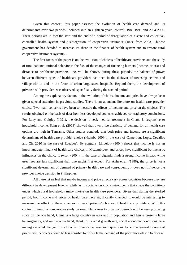
Table 2 describe the evolution of the supply side statistics of health sector and in particular the
evolution of the balance of power between county (and above) hospitals, the townships health centers
and the village clinics. In this official statistics, the data on heath institution measure the total force of
Chinese health supply above the rural village level and do not include village clinics. First, we observe
an increase of supply in number of health institutions and of health professional. Second, relating to
county (and above) hospitals, township centers and village clinics had their force significantly
decreased in line with Chinese urbanization during this period and also with the disengagement of the
state. As exception, however, health professional for township health centers has increased.
5
Table 2: Some indicators of different health institutions
Health institutions Hospitals at county and
above levels
Townships health
centers
Village clinics
1990 2004 1990 2004 1990 2004 1990 2004
Number 208734 296492 14377 18396 47749 41626 803956 551600
Health professional
3897921 4389998 1763086 1904771 358770 402687 1231510 883075
beds 1868905 2364279 722877 668863
Per unit
professional
123 104 7.5 9.7 1.5 1.6
Per unit beds 130 129 15.1 16.1
Professional Per
1000 rural population
0.99 0.77 1.55 1.02
beds Per 1000
rural population
0.81 1.18
Source: 2005 Chinese Health Statistic Yearbook.
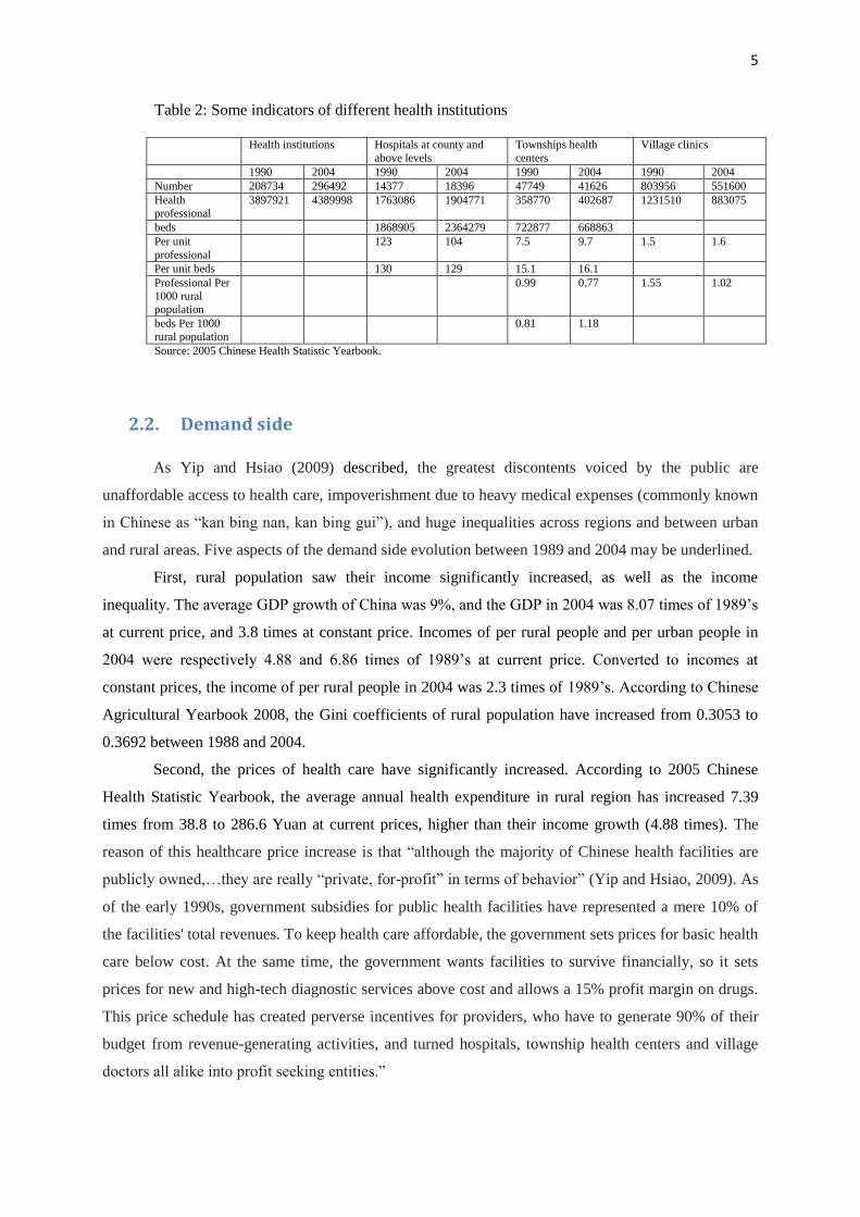
2.2. Demand side As Yip and Hsiao (2009) described, the greatest discontents voiced by the public are
unaffordable access to health care, impoverishment due to heavy medical expenses (commonly known
in Chinese as “kan bing nan, kan bing gui”), and huge inequalities across regions and between urban
and rural areas. Five aspects of the demand side evolution between 1989 and 2004 may be underlined.
First, rural population saw their income significantly increased, as well as the income
inequality. The average GDP growth of China was 9%, and the GDP in 2004 was 8.07 times of 1989‟s
at current price, and 3.8 times at constant price. Incomes of per rural people and per urban people in
2004 were respectively 4.88 and 6.86 times of 1989‟s at current price. Converted to incomes at
constant prices, the income of per rural people in 2004 was 2.3 times of 1989‟s. According to Chinese
Agricultural Yearbook 2008, the Gini coefficients of rural population have increased from 0.3053 to
0.3692 between 1988 and 2004.
Second, the prices of health care have significantly increased. According to 2005 Chinese
Health Statistic Yearbook, the average annual health expenditure in rural region has increased 7.39
times from 38.8 to 286.6 Yuan at current prices, higher than their income growth (4.88 times). The
reason of this healthcare price increase is that “although the majority of Chinese health facilities are
publicly owned,…they are really “private, for-profit” in terms of behavior” (Yip and Hsiao, 2009). As
of the early 1990s, government subsidies for public health facilities have represented a mere 10% of
the facilities' total revenues. To keep health care affordable, the government sets prices for basic health
care below cost. At the same time, the government wants facilities to survive financially, so it sets
prices for new and high-tech diagnostic services above cost and allows a 15% profit margin on drugs.
This price schedule has created perverse incentives for providers, who have to generate 90% of their
budget from revenue-generating activities, and turned hospitals, township health centers and village
doctors all alike into profit seeking entities.”

6
Third, with the disintegration of the Cooperative Medical Service in the 1980s, a great
majority of rural people has lost their cooperative insurance. During this period, various forms of
health insurance were experimented in the rural areas such as the Children Immunization Insurance
(CII), Mother-Infant Medical Insurance (MIMI), and Medical Operation Insurance (MOI). These
experimentations did not change the fact that till 2002, more than 80% of rural people had not been
covered by a medical insurance. In 2003, the Chinese government initiated the New Cooperative
Medical System (NCMS).
Fourth, aging problem appears in rural region: In 1990, the population of more than 65 years
old represented 5.57% of population, this ratio reached 9.07% in 2005, with respectively 9.48 and 8.12%
for rural and urban population (2005 Chinese population statistic yearbook and 2007 Chinese
population and employment statistic yearbook). This means the percent of aging population has nearly
doubled during this period. According to a study by ILO, by 2020, this ratio will reach 14.17% (Yang
and Wang 2010). The health care demand of the older may be stronger than that of younger people and
their preference patterns of healthcare must be different.
Fifth, regional inequality also increased. Table 3 illustrates the evolution of rural per capita net
income at current price of the nine provinces included in our sample. We observe the persistence and
accentuation of this inequality. The ratio between the richest (Jiangsu) to the poorest provinces
(Guizhou) has increased from 2.2 to 2.8 times between 1990 and 2006. The coefficient of variation
(Standard deviation divided by mean value) among them has increased from 0.23 to 0.28.
Table 3 Rural per capita net income of nine provinces in 1990 and 2006 (in current price)
Jiangsu Shandong Liaoning Heilongjiang Hubei Henan Hunan Guangxi Guizhou
1990 959 680 836 760 671 527 664 639 435
2006 6561 4985 4773 4132 3997 3851 3904 3224 2374
Source: 2008 Chinese Countryside Statistic Yearbook
3. Methodology
3.1 Econometric modeling
Econometric model is a mixed multinomial logit model (MMNL) (McFadden and Train 2000;
Borah, 2006), that provides a flexible framework to incorporating both observed and unobserved
factors that influence the provider choice decision. Individual with similar characteristics will also
have similar preferences. In traditional multinomial logit models (MNL), the accent is on the mean
impact of observed variables and all unobserved heterogeneity is classified in error terms. MMNL
allows the parameter associated with each observed variable to vary randomly across individuals, and

7
their variance reflects the unobserved individual-specific heterogeneity. This method decomposes the
mean and standard deviation of one or more random parameters to reveal sources of systematic taste
heterogeneity. This way, in MMNL, the variance in parameters is treated explicitly as a separate
component of the error such that the remaining error is "net" of this variance. Two sources of
unobserved heterogeneity can be considered: features of alternative choices that are not recorded by
the analyst, and unmeasured consumer characteristics that determine preferences (McFadden and
Train 2000).
.
Let the utility of a patient I [1, I ], be a function of health status, h, and non health
consumption, x.
(1)
Health status, h, is determined by the quantity and quality of healthcare (C); other health
inputs, e.g., sanitation, food consumption, etc., (F) and individual attributes, e.g., age, gender,
education, income, etc., (R);
(2)
Health care demand is a function of the price of health care ( ) and the distance to the heath
care provider (D). The importance of D is that distance not only implies costs to access, but also
reflects the reputation and quality of providers.
(3)
Finally, F, the other health input is a function of expenditure on these inputs ( ).
(4)
With equations (1) to (4), we get the indirect utility function in the case where individual I
choices the health care provider j in which is the budget for non health consumption (y
is income).
(5)
Among the alternative health care providers the patient will choose that which maximizes his
indirect utility function. This is expressed by the equation (6).
, if
, otherwise (6)

8
To make the model amenable to econometric estimation we must define a functional form of
the above indirect utility function. This is expressed by the equation (7) in which the first term on the
right is the deterministic component of utility in function of the above defined four types of attributes
and the second term is a disturbance term. The term is unobserved and is treated as one part of
error term.
(7)
The equation (7) must be parameterized to allow estimation. The first term can be rewritten as:
(8)
The X variables are patient specific characteristics such as age, marital status, insurance status,
income and so on. The Z variables are alternative health provider specific characteristics such as
distance, price, healthcare quality, and so on. In our above defined variables, we have
(9)
The variable p, the healthcare price, and D, the distance of healthcare provider are two specific
variables, and the y, income and R, individual attributes other than income are patient specific
variables. In our econometric estimations, p and D are kept constant across options while y and all
components of R vary across options.
If the equation (9) is estimated with MNL, the basic form of the multinomial logit model, with
alternative specific constants and attributes (x represents both z and x variables in the equation
(8) will be:
(10)
The difference between MMNL and MNL is that in the former one part of the coefficients are
random while in the latter all coefficients are non random. In equation (10) is composed of with
(11)
where is the population mean, is the individual specific heterogeneity, with mean zero
and standard deviation one, and is the standard deviation of the distribution of around . The
elements of are distributed randomly across individuals with fixed means. A refinement of the
model is to allow the means of the parameter distributions to be heterogeneous with observed data .
This would be a set of choice invariant characteristics that produce individual heterogeneity in the
means of the randomly distributed coefficients so that selecting subsets of pre-specified variables to
interact with the mean and standard deviation of random parameterized attributes.

9
In our case, we set both price and distance to healthcare providers as random variables. First,
they may have a substitutive feature, in other words, when people have more choice in prices, they
may less care about the distance. By contrary, when they have less choice in prices, they may prefer a
less distant provider. Secondly, distance may reflect the reputation and quality of providers. It will be
interesting to estimate the heterogeneity in their preference for both price and distance. In particular,
we are interested in examination of their interaction with some variables of type w in Equation (11).
Here will be composed of four variables: income (asset), insurance, severity of the illness and rural
labor ratio of the village (we will return to this point later).
Given that are individual specific, will reflect unobserved random disturbances - the
source of the heterogeneity. Thus, as stated above, in the population, if the random terms are normally
distributed,
(12)
The equation (12) has useful empirical implication and we will return to this in application.
Finally, to make our model more realistic, we will allow the two random parameters (p and D) to be
correlated.
3.2. Data
Data are from the CHNS database, edited by the Carolina Population Center (CPC, University
of North Carolina). The survey covers about 16,000 individuals from more than 3,000 households
(about two third from rural and one third from urban population) in nine representative provinces. It is
a longitudinal survey with seven waves (1989, 1991, 1993, 1997, 2000, 2004, 2006), covering a period
of 18 years.
As we have explained, over this long period, we are interested in the start and end periods of
the liberalization of health care system. We have chosen to merge the data 1989, 1991 and 1993 in the
first sample and the data of 2004 and 2006 in the second sample with two criterion: 1/ the size of the
sample: given in the first period the number of the surveyed being ill is smaller than in the second
period, we include three time periods for the first sample while two time periods in the second sample;
2/ within each sample, we keep attention to be sure that income, health care prices and supply
conditions are not significantly changed. From this data source, we get 2117 rural people that declared
to be ill in 1989, 1991 or 1993, and 2594 people that declared to be ill in 2004 or 2006.
Table 4 presents all variables we will use and their definitions. In this table, the first five items
from Village-C to Self-Care are choice set of healthcare providers, and the following five items on
price and distances are choice specific variables; all the rest are patient specific variables. The last
three items are used to take into account the environmental features of the patients: rural population

10
rate is a proxy of the development level of the village, village size is a proxy of the village clinic‟s size,
and finally suburb reflects the proximity of the village to urban medical infrastructure.
Table 4 Variable definitions
Village-C (V) =1 if the choice of treatment is village clinic; =0 otherwise.
Town-C (T) =1 if the choice of treatment is township center; =0 otherwise.
County-H (C) =1 if the choice of treatment is county or higher level city hospital; =0 otherwise.
Oth_Type (O) =1 if the source of treatment is pharmacy, private clinic, private hospital and other clinic;
=0 otherwise.
Self-Care =1 if self-treatment is chosen; =0 otherwise. Medical expense at constant price of alternative j; j=V, T, C, O: the four choices of
treatment after eventual reimbursement by insurance. =1 if distance <0.5 km; =0 otherwise; j=V, T, C, O. =1 if distance >=0.5 km & <3; =0 otherwise; j=V, T, C, O. =1 if distance >=3 km &<10km; =0 otherwise; j=V, T, C, O. =1 if distance >=10 km; =0 otherwise; j=V, T, C, O.
Age Age of the patient in years.
Female =1 if the patient is female; =0 if male; =that of the decider: the Household chief if patient‟s
age<16.
Marital =1 if the patient is married; =0 otherwise; =that of the Household chief if patient‟s age<16.
Edu_years =1 graduated from primary school;=2 lower middle school degree;=3 upper middle school
degree;=4 technical or vocational degree;=5 university or college degree;=6 master‟s
degree or higher. =that of the Household chief if patient‟s age<16.
Urb_job =1 if the patient‟s job is not farmer; =0 otherwise; =that of the Household chief if patient‟s
age<16.
Farmer =1 if the patient‟s job is farmer; =0 otherwise; =that of the Household chief if patient‟s
age<16.
No_job =1 if the patient has not job;=0 otherwise;=that of the Household chief if patient‟s age<16.
No_insured =1 if the patient is not insured; =0 otherwise.
Urb_Insu =1 if the patient‟s insurance is one of the following types: commercial, free medical,
workers compensation, for family member, urban employee: passway model, urban
employee: block model, Urban Employee: Catastrophic disease; =0 otherwise.
Cooperative =1 if the patient‟s insurance type is cooperative; =0 otherwise.
Oth_insu =1 if the patient‟s insurance is other than Urban_insu and Cooperative (they include among
others Health insurance for women and children, EPI (expanded program of immunization)
insurance for children); =0 other wise.
Severity =1 if the illness or injury not severe; =2 somewhat severe; =3 quite severe;
Fever =1 if individual suffered from fever; =0 otherwise.
Chronic =1 if individual suffered from chronic diseases; =0 otherwise.
Oth_deas =1 if individual suffered from diseases other than fever and chronic diseases; =0 otherwise
Hhsize The number of the household members.
Income The annual per capita income at constant price of the household multiplied by 10-3
.
Asset The annual per household value of the asset index 10-3
.
Rural popu. rate The share of the rural employees in total labor of the village
Village_size The household number of the village multiplied by
Suburb =1 if the village is near a city; =0 otherwise.
From the CHNS database, we get household annual income at constant price. The variable
“income” will be used to estimate the impact of income. However, we consider that income only
partially reflects the economic and financial states of households and individuals. Furthermore, linked

11
with the specificities of farm activities, their incomes are often too volatile and some households have
reclaimed their income negative (we have tried to remedy this by approaching the actual income to
“permanent income”, with the criterion that when for the same household if their incomes in the two
previous time periods are higher, we replace the actual income by the highest income). With this
method, the problem is just partially solved since in our sample, one part of household lack continuous
data and the data in the start year (1989) cannot be adjusted. Thus we judge necessary to constitute
asset index of households and alternatively use income and asset to measure the income effect, or
more exactly wealth effect. We use the following items for asset index: 1. drinking water (4 choices);
2. toilet facilities (8 choices); 3. kind of lighting (5 choices); 4. kind of fuel for cooking (8 choices); 5.
type of ownership of apartment/house (6 choices); 6. ownership of electrical appliances and other
goods (the number of appliances vary between 15 to 18 according to the periods of survey, and this
information is absent only in 1989). 7. means of transportation (5 choices). 8. type of farm machinery
(5 choices). 9. Household Commercial Equipment (6 choices). We use principal components analysis
to derive weights for each time periods (Filmer and Scott 2008). The coefficients of correlation
between obtained ASSET and INCOME are 0.29 for periods 89-93 and 04-06, both significant at 1%.
Another necessary work is to impute the missing prices of heath cares. Since MMNL requires
the prices of all the alternative providers, while in the survey only the prices of the providers that
patients visited were recorded. So, the prices of alternative providers that the patient did not visit need
to be imputed. Following Gertler et al. (1987) and Borah (2006), we use Stata ICE program created by
Royston (2004) to impute the lacked price data. All reported prices are converted at constant price
using the weights provided by CHNS data provider. ICE imputes missing values by using switching
regression, an iterative multivariable regression technique. The chosen predictors of price include
variables Age, Female, Marital, Edu_years, Urb_job, Farmer, Income, Severity, Year, Province,
Urb_Insu, Cooperative, Oth_insu, Fever, Chronic, and finally hospitalized (=1 if hospitalized; =0
otherwise). The regressions are separately operated according to the choices V (village clinic), T
(township center), C (county or city center) and O (other center, see Table 4). The descriptive statistics
of imputed plus actual prices by type of providers are presented in Table 5.
In Table 5, the first part is that the sample distribution by province. The most significant
difference between the two samples is that Heilongjiang is present only in sample 04-06. Since
according to Table 3, Heilongjiang is a province with development level at the middle range among
the 9 provinces, we consider that its inclusion in the sample 2004-2006 will not bias the comparability
of the results.
When comparing the two samples, the choice for village clinic (more than 50% between 1989
and 1993) has considerably reduced (to 22%) and the choice on self-care has significantly increased
(from19% to 35%). These may be produced by two facts. As shown above, since this period, the force
of small rural health care providers has significantly weakened while that of urban large hospital

12
reinforced, thereby leading to the decrease of choice to village clinic. The aging of population (second
period) may cause the choice of self-care.
Between the two periods, the increase of medical expenses (P_V, P_T, P_C and P_O) is less
than 100%, and lower than the published statistics. According to 2005 Chinese Health statistic
Yearbook, between 1995-2004 the per outpatient medical expense at county level hospital increased
from 24.8 to 77.2 Yuan at current price, and the corresponding per inpatient medical expense from
880.6 to 2087.2 Yuan. Even converted to expense at constant price, they are higher than ours. But ours
are medical expenses after the reimbursements by insurance. With more than 1/3 of patients that have
been beneficiaries of insurance in period 04-06, this may sensitively reduced the real paid medical
expenses. The variation of the medical prices in the second period is smaller than that in the first
period. The coefficients of variation (SD/mean) of P_V, P_T and P_C have reduced from 1.11, 1.11
and 1.37 to 0.82, 0.82 and 0.92. As we know a larger heterogeneity of price allows the consumers a
larger possibility of choice, this evolution may have an impact on the demand structure.
Fourth, there is an important difference in age between the two samples. While for the sample
89-93, to insure the sufficient size of the sample, we have kept the patients that were younger than 18
years old, while for the sample 04-06, all surveyed patients are above 18 years old. Consequently the
average age of the sample 89-93 is much lower than that of 04-06. We argue that this fact has not
significant impact on the objective of our study. As noted in the end of the Table 5, as the accent of
this study is on the choice decider, for all patients under 16 years old, sex, marital and edu_years, job
types are all on household chiefs‟. The only constraint for our study is that we cannot directly compare
the coefficients of age of MMNL regressions of the two samples. This difference in age has not a bias
on our study on aging problem. If we remove these young patients from the sample 89-93, there
remain 1457 observations and their mean, SD, Min and Max are 44.47, 15.42, 18 and 92 respectively.
Comparing these with the sample 2004-2006 in which all patients are 18 years old and above, we
observe the aging problem: since the surveys were operated roughly in the same places, as the people
get old and the aging people are more frequent to be ill, the mean age of the people get more than 10
years older during a period of 14 years (1991-2005, the mean time points of the two periods). Without
accounting the patients of less than 16 years old in the sample 89-93, the % of aging patients (older
than 60) was only 18.6% while this percent was 41.1% in the sample 04-06. In other words, in the
sample 89-93, that fact of including or not the younger patients, the aging problem was not a concern,
while in 04-06, it has become a concern. Therefore their comparison has implication into aging issue.
Fifth, in line with the evolution of age, there is also a significant difference on employment.
While in the sample 89-93, only 13% patients have declared without job, this proportion has increased
to 50%. We have checked that the mean age of the patients without job is 62.3 years old. As expected,
the majority of them are retired aging people.

13
Sixth, as the period 1989 and 2003 is the beginning and the end of a period without insurance,
the sample 2004-2006 (in which at least 1/3 rural households have had cooperative insurance) allow us
to measure the impact of restoration of rural insurance.
Seventh, as explained, we are concerned to measure the impacts of permanent income, or
wealth on healthcare choice. Thus we choose asset as principal, and income as secondary variable.
Inequality measured in asset and in income is, however, different. With our samples, mean income at
constant price has increased 2.57 times, roughly in line with national level (2.3), and inequality has
increased from 0.78 to 1.14 in terms of coefficient of variation. Asset has increased 3.42 times, higher
than income increase. But coefficient of variation of the asset in period 04-06 has significantly reduced.
This is not unusual for two reasons: in our principal component estimations, all items have been
equivalently weighted (for example, the access to water is given equal importance with the ownership
of the house). This leads a sensitive reduction of inequality in the favor of the poor. While asset index
is closer to permanent income, it is well-known that permanent income is much less unequal than real
income due to accumulated and smoothing effects. As the households‟ income inequality in our
sample is closer to national level income inequality, we use income as complementary variable to
observe eventual difference between asset and income. If their impacts are significantly different, it is
quite possible that larger inequality existing in income variable plays a role. Otherwise we can ignore
the impact of inequality on healthcare choice.
Table 5 Descriptive statistics
1989-1993 (n=2117) 2004-2006 (n=2594)
Mean SD Min Max Mean SD Min Max
Sample distribution
Liaoning 0.09 0.29 0 1 0.12 0.32 0 1
Heilongjiang 0 0 0 1 0.07 0.25 0 1
Jiangsu 0.14 0.35 0 1 0.12 0.32 0 1
Shandong 0.06 0.24 0 1 0.09 0.29 0 1
Henan 0.19 0.39 0 1 0.13 0.33 0 1
Hubei 0.12 0.33 0 1 0.10 0.30 0 1
Hunan 0.09 0.29 0 1 0.11 0.32 0 1
Guangxi 0.19 0.40 0 1 0.16 0.37 0 1
Guizhou 0.11 0.31 0 1 0.10 0.30 0 1
Village-C 0.51 0.50 0 1 0.22 0.41 0 1
Town-C 0.23 0.42 0 1 0.14 0.35 0 1
County-H 0.08 0.27 0 1 0.18 0.39 0 1
Oth_Type 0 0 0 1 0.11 0.32 0 1
Self-Care 0.19 0.39 0 1 0.35 0.48 0 1
P_V 0.066 0.073 0 0.477 0.096 0.079 0 0.598
P_T 0.140 0.156 0 0.859 0.207 0.169 0 1.166
P_C 0.425 0.579 0 3.506 0.651 0.597 0 3.808
P_O 0.204 0.318 0 3.972
Dist0_V 1 0 1 1 1 0 1 1
Dist0_T 0.39 0.49 0 1 0.48 0.50 0 1
Dist1_T 0.42 0.49 0 1 0.36 0.48 0 1
Bdist2_T 0.19 0.40 0 1 0.15 0.36 0 1
Cdist3_T 0 0 0 0 0 0 0 0
0dist0_C 0.16 0.37 0 1 0.23 0.41 0 1
Dist1_C 0.22 0.41 0 1 0.22 0.42 0 1
Dist2_C 0.21 0.41 0 1 0.25 0.43 0 1
Dist3_C 0.41 0.49 0 1 0.30 0.46 0 1
Dist0_O 0.63 0.48 0 1
Dist1_O 0.26 0.44 0 1
Dist2_O 0.09 0.29 0 1

14
Dist3_O 0.02 0.15 0 1
Age 32.29 22.31 1 92 55.88 15.12 18 97
Female 0.40 0.49 0 1 0.57 0.49 0 1
Marital 0.87 0.33 0 1 0.80 0.40 0 1
Edu_years 0.79 1.01 0 5 1.17 1.21 0 6
Urb_job 0.26 0.44 0 1 0.13 0.35 0 1
Farmer 0.61 0.49 0 1 0.35 0.48 0 1
No_job 0.13 0.34 0 1 0.51 0.50 0 1
No_insured 0.81 0.40 0 1 0.64 0.48 0 1
Urb_Insu 0.11 0.32 0 1 0.10 0.30 0 1
Cooperative 0.03 0.16 0 1 0.25 0.43 0 1
Oth_insu 0.06 0.23 0 1 0.01 0.10 0 1
Severity 1.67 0.68 1 3 1.7 0.67 1 3
Fever 0.46 0.50 0 1 0.26 0.44 0 1
Chronic 0.10 0.30 0 1 0.34 0.47 0 1
Oth_diseases 0.44 0.50 0 1 0.40 0.49 0 1
Hhsize 4.50 1.50 1 13 3.66 1.69 0 13
Income 2.74 2.14 0.45 22.20 7.03 8.03 0.18 210.95
Asset 0.35 0.76 -1.05 3.08 1.20 0.96 -0.62 3.87
Rural popu rate 0.54 0.33 0 1 0.41 0.30 0 1
Village_size 0.66 0.72 0.03 6.00 1.01 1.19 0.04 8.00
Suburb 0.24 0.43 0 1 0.24 0.43 0 1
Note: In 89-93, 29.9% (632 of 2117) of observations are under 16 years old. As the accent of this study is on the
decider, in these cases, sex, marital and edu_years, job types are all on household chiefs‟. Therefore there are
significant differences in means of these indicators between the two periods.
4. Results
In the followings, we present and analyze the results of MMNL estimations. Table 6 and 7
present the results of MMNL estimations with respectively asset and income variables. As we have
explained, given the importance of the measurement of income effect, we use alternatively the two
variables to obtain a more complete view given that one closer to permanent income and another
reflects better increasing inequality. But to save space, in Table 7, for all patient specific variables
(except income), we remove all variables of which the results are the same with that in Table 6 with
criterion of the sign and significance of their coefficients. For example, if woman is a variable of
which the coefficients have the same sign in both table, and both, significant or insignificant, we will
not show it in Table 7. On the contrary, as age in 04-06 is not significant for the choice of Oth-type in
Table 6, while it is significant in Table 7, this result will be kept in Table 7. This way, all results of
patients specific variables we have kept are those that are different with the results in Table 6.

15
Table 6 Mixed Logit Regression results with asset as wealth indicator
89-93 04-06
Village-C Town-H County-H Village-C Town-H County-H Oth_Type PRICE -3.10 (-3.24)*** -1.73 (-2.83)***
Dist1 -1.15 (-2.46)** -1.40 (-2.77)***
Dist2 -1.61 (-2.77)*** -1.69 (-2.43)** Dist3 -1.55 (-1.51)
-2.69 (-3.05)***
intercept 0.21 -0.52 -0.90 -1.05 -0.93 0.27 -0.80 (0.44) (-0.86) (-1.01) (-2.04)** (-1.35) (0.37) (-1.09)
Age -0.02 -0.03 -0.02 -0.0005 -0.01 -0.01 -0.01
(-6.99)*** (-6.17)*** (-2.79)*** (-0.09) (-0.83) (-2.36)* (-1.62) Edu_years 0.01 -0.04 0.04 -0.06 -0.12 -0.11 -0.08
(0.14) (-0.45) (0.37) (-0.85) (-1.46) (-1.58) (-1.04)
Women 0.27 0.20 0.21 0.08 -0.04 -0.03 -0.08 (2.00)** (1.24) (0.92) (0.60) (-0.26) (-0.19) (-0.49)
Hhsize -0.01 0.06 -0.002 -0.01 0.01 -0.01 -0.12
(-0.34) (1.15) (-0.03) (-0.20) (0.20) (-0.16) (-2.21)**
Asset 0.25 0.09 -0.37 -0.12 0.01 0.19 0.02
(2.00)** (0.51) (-1.32) (-1.43) (0.09) (1.22) (0.12)
Severity 0.45 0.74 0.77 0.39 0.77 0.46 0.45 (4.45)*** (4.86)*** (3.30)*** (3.89)*** (5.65)*** (2.60)*** (3.24)***
Marital 0.45 0.45 0.43 0.08 0.16 0.39 0.19
(2.48)** (2.03)** (1.40) (0.49) (0.81) (2.12)** (0.95) Urb_Insu 0.25 0.13 -0.09 -0.42 -0.07 0.29 0.06
(0.91) (0.34) (-0.19) (-1.41) (-0.19) (0.88) (0.19)
Cooperative 0.64 0.69 0.94 0.24 -0.05 -0.31 0.11 (1.32) (0.89) (0.98) (1.45) (-0.19) (-0.78) (0.40)
Urb_job 0.30 0.16 0.09 -0.04 0.07 -0.67 -0.30
(1.29) (0.57) (0.26) (-0.18) (0.28) (-2.74)*** (-1.13)
Farmer 0.19 -0.10 -0.22 0.09 -0.07 -0.42 -0.08 (0.89) (-0.42) (-0.64) (0.59) (-0.40) (-2.03)** (-0.40)
Fever -0.23 -0.51 -0.75 0.90 0.38 -0.81 0.69 (-1.71)* (-3.09)*** (-3.17)*** (6.03)*** (2.02)** (-3.57)*** (3.75)***
Chronic 0.11 -0.23 0.01 -0.09 -0.14 -0.17 -0.43
(0.49) (-0.87) (0.02) (-0.60) (-0.82) (-1.09) (-2.27)** Rural labor 0.60 0.15 0.04 0.62 -0.05 -0.29 -0.27
(1.97)** (0.34) (0.05) (2.01)** (-0.11) (-0.41) (-0.62)
Village_size 0.28 0.04 0.33 -0.10 0.03 0.08 -0.10 (2.26)** (0.24) (2.09)** (-1.17) (0.39) (1.29) (-0.95)
SUBURB 0.07 -0.32 0.17 -0.42 -1.55 -0.35 -0.08
(0.27) (-1.08) (0.39) (-1.78)* (-5.36)*** (-1.21) (-0.29) Jiangsu -0.09 0.74 0.20 -0.33 -0.86 -0.04 -0.44
(-0.34) (2.41)** (0.46) (-1.24) (-2.46)** (-0.12) (-0.97)
Shandong 0.09 0.90 1.09 -0.02 -0.47 0.25 0.04 (0.25) (2.27)** (2.09)** (-0.09) (-1.36) (0.66) (0.09)
Liaoning -1.09 -0.87 -0.96 -1.82 -1.08 -0.77 -0.28
(-4.14)*** (-2.64)*** (-1.87)* (-6.16)*** (-3.56)*** (-2.38)** (-0.71) Heilongjiang -0.48 -0.37 0.51 -0.58
(-1.68)* (-0.93) (1.43) (-1.09)
Henan -0.16 0.10 -0.26 0.66 0.73 1.10 1.61 (-0.66) (0.33) (-0.60) (2.55)** (2.24)** (3.17)*** (4.00)***
Hunan 0.21 0.38 0.75 -0.92 -0.22 -0.59 0.35
(0.70) (1.06) (1.59) (-3.39)*** (-0.74) (-1.66)* (0.87) Guangxi -0.09 0.03 0.15 -0.27 -0.20 0.57 0.89
(-0.39) (0.12) (0.38) (-1.11) (-0.67) (1.95)* (2.24)**
Guizhou -0.45 -0.72 -0.94 -1.45 -0.87 -0.50 0.48
(-1.82)* (-2.25)*** (-2.05)** (-5.38)*** (-2.65)** (-1.55) (1.20)
1991 0.15 0.30 -0.17
(0.95) (1.61) (-0.63) 1993 0.15 0.36 -0.04
(0.84) (1.68)* (-0.14)
2006 0.38 0.02 0.22 0.08 (2.77)*** (0.12) (1.42) (0.45)
Heterogeneity in mean parameters
P:Asset 0.06 (0.19) -0.21 (-1.31)
P:Urb_Insu 0.42 (0.72) 0.49 (1.15) P:Cooperative -1.84 (-1.36) 0.14 (0.50)

16
P:Severity 0.77 (2.55)** 0.76 (3.59)*** P:Rural labor -0.41 (-0.53) -0.17 (-0.34)
Dist1: Asset 0.40 (2.08)** 0.19 (1.45)
Dist1:Urb_Insu 0.08 (0.20) 0.09 (0.25) Dist1:Cooperative 0.25 (0.31) -0.01 (-0.03)
Dist1:Severity 0.19 (1.10) 0.19 (1.13)
Dist1:Rural labor 0.99 (2.20)** 0.24 (0.56) Dist2: Asset 0.36 (1.41) 0.29 (1.65)*
Dist2:Urb_Insu 0.93 (1.79)* 0.32 (0.67)
Dist2:Cooperative 0.28 (0.30) 0.13 (0.40) Dist2:Severity 0.36 (1.76)* 0.46 (2.13)*
Dist2: Rural labor 0.49 (0.85) -0.54 (-0.88)
Dist3: Asset 0.49 (1.33) 0.07 (0.33) Dist3:Urb_Insu -0.08 (-0.09) -0.26 (-0.45)
Dist3:Cooperative 0.32 (0.26) -0.14 (-0.31) Dist3:Severity 0.34 (1.10) 0.71 (2.80)***
Dist3: Rural labor -0.02 (-0.02) 0.41 (0.53)
SD of parameter
distributions
PRICE 1.76 (4.71)*** 1.55 (4.79)*** Dist1 0.26 (0.39) 1.17 (2.95)***
Dist2 0.60 (1.19) 1.23 (2.56)**
Dist3 0.95 (1.31) 0.95 (1.67)*
N 2117 2594
Log-like -2339.81 -3452.60 LR Chi Squared 1189.95 1444.56
McFadden Pseudo R2 0.2027 0.1730
Note: t-Statistics in parentheses. *** indicates significance at 1%; ** indicates significance at 5%; and *
indicates significance at 10%.
Table 7 Mixed Logit Regression results with income as wealth indicator 89-93 04-06
Village-C Town-H County-H Village-C Town-H County-H Oth_Type
PRICE -2.8 (-3.01)*** -1.98 (-3.68)*** Dist1 -1.11 (-2.29)** -1.04 (-2.64)***
Dist2 -1.46 (-2.40)** -1.43 (-2.56)**
Dist3 -0.85 (-0.82) -2.32 (-3.78)*** intercept -1.50
(-1.68)*
Age -0.01 (-1.74)*
Income 0.02 -0.05 0.003 -0.004 -0.01 0.02 -0.01
(0.74) (-1.02) (0.04) (-0.38) (-0.63) (1.03) (-0.69) Hunan -0.48
(-1.46)
Guizhou -0.60 (-1.87)*
Heterogeneity in
mean parameters
P:Income -0.03 (-0.31) -0.01 (-0.81)
Dist1: Income 0.14 (2.28)** -0.01 (-0.07)
Dist1:Rural labor 0.60 (1.50) Dist2: Income 0.11 (1.52) 0.05 (2.22)**
Dist2:Severity 0.33 (1.61)
Dist3: Income 0.05 (0.54) -0.04 (-1.50)
SD of parameter
distributions
PRICE 1.73 (4.59)*** 1.45 (5.12)***
Dist1 0.32 (0.39) 1.14 (3.22)***
Dist2 0.64 (1.32) 1.12 (2.57)** Dist3 0.67 (0.66) 0.76 (2.00)**
N 2117 2594 Log-like -2342.20 -3454.48
LR Chi Squared 1185.18 1440.80
McFadden Pseudo R2 0.2019 0.1726
Note: t-Statistics in parentheses. *** indicates significance at 1%; ** indicates significance at 5%; and *
indicates significance at 10%.
17
4.1. Price effects
Assuming individual rationality, the impact of the healthcare prices on the choice among the
healthcare providers must be negative. The higher the price associated with a provider, the less likely
the later will be chosen. From Table 6, according to MMNL method, in both periods there are clear
price effects, the estimated means for the two periods are respectively -3.1 and -1.73 and both
significant at 1%, indicating negative price effect but a weaker effect in 04-06. The „Standard
Deviation of Parameter Distributions‟ section of Table 6 gives the standard deviations of the relevant
coefficients. As we know, in standard MNL regression, individual heterogeneity is not treated and all
unobserved heterogeneity factors are simply grouped in error term. In MMNL, one part of coefficient
of price variable is allowed to randomly vary around the mean value. This part reflects the unobserved
individual specific heterogeneity. With the SD of 1.76 and 1.55 of the two periods and both significant
at 1%, we conclude that there exists heterogeneity in price preferences. In Table 7 with income as
wealth indicator, these values are slightly different, but the tendency is the same with respect to sign
and significance.
MMNL provides more information than MNL, in that the MMNL estimates the extent to
which patients differ in their preferences for providers. Therefore, the interest of MMNL approach is
to analyze the observed and unobserved heterogeneity on the impact of price on choices. While the
„Standard Deviation of Parameter Distributions‟ reflects the extent of unobserved heterogeneity, the
“heterogeneity in mean parameters” reflects the observed heterogeneity on the impact of price choices
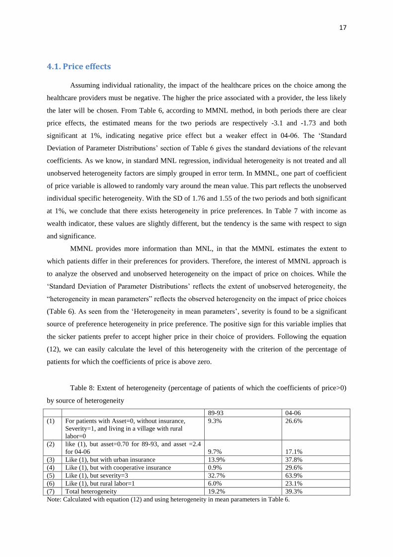
(Table 6). As seen from the „Heterogeneity in mean parameters‟, severity is found to be a significant
source of preference heterogeneity in price preference. The positive sign for this variable implies that
the sicker patients prefer to accept higher price in their choice of providers. Following the equation
(12), we can easily calculate the level of this heterogeneity with the criterion of the percentage of
patients for which the coefficients of price is above zero.
Table 8: Extent of heterogeneity (percentage of patients of which the coefficients of price>0)
by source of heterogeneity
89-93 04-06
(1) For patients with Asset=0, without insurance,
Severity=1, and living in a village with rural
labor=0
9.3%
26.6%
(2) like (1), but asset=0.70 for 89-93, and asset =2.4
for 04-06 9.7% 17.1%
(3) Like (1), but with urban insurance 13.9% 37.8%
(4) Like (1), but with cooperative insurance 0.9% 29.6%
(5) Like (1), but severity=3 32.7% 63.9%
(6) Like (1), but rural labor=1 6.0% 23.1%
(7) Total heterogeneity 19.2% 39.3%
Note: Calculated with equation (12) and using heterogeneity in mean parameters in Table 6.

18
Table 8 makes evidence of the price heterogeneity imputed to four observed sources. As seen
in line (1), the probability for a patient with asset=0 (note that it is not equivalent to absence of asset
since asset index can be negative), without insurance, severity=1, and living in a village with rural
labor=0, to accept the coefficient of price>0 is 9.3% in 89-93, and this probability has increased to
26.60, indicating a significant rise of price heterogeneity. Line (2) shows the influence of asset to price
preference. As the mean value of asset is 0.35 for 89-93 and 1.2 for 04-06, we use those with
asset=0.70 in 89-93 and asset =2.4 to compare with those with asset=0. In 89-93, the probability to
prefer coefficient of price>0 has just slightly increased from 9.3% to 9.7%, indicating a weak impact
of asset on price preference. In 04-06, the direction of this impact is even inversed. The probability for
richer patient to prefer coefficient of price>0 is even weaker. In our analysis of elasticity of price
following Table 9, we will return to explain it. Line (3) indicates that patients with urban type
insurance have higher price heterogeneity. Line (4) show that while in 89-93 the probability for price
heterogeneity for patients with cooperative insurance (0.9%) is even lower than for patients without
cooperative insurance (9.3%), while in 04-06, this probability becomes higher (29.6% versus 26.6%).
Line (5) shows that the most important source of price heterogeneity is the severity of illness. For the
patients declaring their illness quite severe, their probability to accept higher prices are sensibly
increased. Line (6) shows that for the patients living in less developed villages (with higher proportion
of rural labor), their price rationality is stronger. Finally the above analysis cannot give us an overall
assessment of the price heterogeneity. To obtain this, line (7) is calculated on the basis of MMNL
estimations with same variables but without heterogeneity in mean parameters. This way, the SD of
parameter distribution of price reflects total observed and unobserved heterogeneity. Heterogeneity in
preference of price has sensibly increased and the % of patients that has price coefficient>0 increased
from about 20 to 40 %.
We have shown that price effect in choice exists in both periods and it is weaker in 04-06, and
heterogeneity in price preference has meaningfully increased in the second period. This heterogeneity
has been analyzed trough the SD of parameter distribution of price and through heterogeneity in mean
parameters. Another method is to calculate price elasticity by type of provider and asset range between
the two periods. This method will provide more detained information. In Table 9, price elasticity is
calculated under MMNL using exactly the same variables than in Table 6 (and Table 7 if using income
as wealth indicator). In the first half of Table 9, we observe that in all cases except for county hospital
in 04-06, price elasticity by provider type is negative. This elasticity by provider type is lower in 04-06
than in 89-93, and becomes positive in the highest level provider type: county hospital. This more
refined result is in line with the above analysis on MMNL results.

19
Table 9 Price Elasticity of choice by provider type and by asset range in two periods
89-93 04-06
V T C V T C O
Price (using asset) -0.0591 -0.1456 -0.0797 -0.0164 -0.0861 0.0364 -0.0438
Price (using income) -0.0585 -0.1458 -0.0730 -0.0153 -0.0878 0.0308 -0.0467
By asset range
Asset Q1 -0.1399 -0.1819 -0.7368 -0.0030 -0.0350 0.1863 -0.0083
Asset Q2 -0.0787 -0.1677 0.4014 -0.0525 -0.2424 0.1943 -0.1835
Asset Q3 -0.1193 -0.1774 0.1391 -0.0944 -0.0776 -0.0914 -0.0359
Asset Q4 -0.0291 -0.0998 0.0476 -0.0190 -0.0189 -0.0306 -0.0155
Note: Q1 is the first income quartile, Q2 is the second income quartile and so on.
4.2. Distance effects
The second random variable in our MMNL models is distance of health care providers. We
distinguish four levels of distance: from Dist0 to Dist3 (see their definitions in Table 5). From Table 5,
we know that all village clinics have Dist0, and in general the larger the hospitals the farer their
distance. We expect that other things equal, patients prefer closer to farer healthcare providers. In
Table 6, as in Table 7, except Dist3 in 89-93, all Distance dummies are significantly negative,
indicating that relating to health care providers situated at Dist0, those with longer distance are less
likely to be chosen. In comparison between the results of 89-93 and 04-06, we observe that impact of
distance is stronger in 04-06 with larger coefficients in absolute values, and the coefficients are
increasing, always in absolute values, as distance prolonged. In particular, the most significant
difference between 89-93 and 04-06 is that in the former case, the Dist3 (the distance longer than
10km) is not significant while in the later case, the providers of Dist3 are least likely chosen in
comparison to all other providers with the distances less than 10km. This leads us to conclude that in
04-06, patients have stronger preference to visit a health facility that is located at a shorter distance.
This result seems to confirm the hypothesis we tend to check: when patients have less
possibility to discriminate providers by price, they increase their preference in choice by distance.
With the general increase of price level, and in particular price determination has more and more ex-
post feature, in other words in 04-06, the choices by price become more uncertain, patients rationally
return to choose in distance that is known. For instance, when A is expensive and close and B is
cheaper and far, to the extent that transport costs and opportunity cost of time are low, a lot of people
prefer to go to B. But in 04-06, when the prices of A and B are not distinctly different, the choice of
distance is privileged (note that the fees for transportation are not included in price of health care,
hence the distance reflects also to some extent the transport costs), patients will prefer to go to A..
Another fact is that while in 89-93, heterogeneity of distance in term of SD of parameter
distribution is weak and not significant, this heterogeneity becomes stronger and all significant in 04-
06. In this case analyzing some observed sources of heterogeneity using “heterogeneity in mean
parameters” is meaningful only to the period 04-06. We observe that distance seems to matter less the
sicker the patients. This reflects the fact that sicker people tend to choose more reputed providers, and

20
therefore, willing to travel greater distance. Asset increases in general distance heterogeneity in all
Dist1 to Dist3, while its contribution to distance heterogeneity in providers farther than 10km is very
weak. This means that the richer patients are not exigent in the choices of near distance, while they are
more dislike to long distance providers just as poorer patients. The coefficients of rural labor indicate
that the patients living in less developed villages are less care to distance for the providers with Dist1
and Dist3, while they are more careful to distance for providers with Dist2 (between 3 to 10 km). The
patients with urban insurance are stronger distance requirements for providers of farther than 10 km,
while they are less care with distance for providers of less than 10 km. Roughly the same tendency is
observed for the patients with cooperative insurance.
4.3. Wealth effects
Wealth effect on the choice of healthcare providers means that wealth positively impacts the
choice of providers, in other word, the extent to which richer patients have access to health care is
larger than poorer patients. The poorer patients are more likely to be excluded from health care. With
the estimation results, we are allowed to use two complementary ways to test wealth effect: first, to
check the coefficients of asset and income in MMNL in Tables 6 and 7; second, to check the price
elasticity by asset range shown in Table 9.
From Table 6, in 89-93, the coefficient of asset for village clinic is significantly positive while
in 04-06, asset is insignificant for all choices. In other words, the patients with more assets tend to
choose village clinic than patients with low asset level with respect to self-care. Given that in 89-93,
the choice of village clinic represents 51% of the total choices, we conclude that while there existed
wealth effect in 89-93, this effect is absent in 04-06. Using income as explanatory variable in the place
of asset, however, this effect is absent for both periods.2 It means that while in 89-93, wealth level
plays a role in some choices, in 04-06, it has no longer significant impact on the choice of healthcare
providers. How to interpret this result? First, during this period in line with the increase of about 4
times of GDP at constant price, and with the increase of the share of health expenditure in GDP from
about 4% to more than 5.5%, there is a significant improvement of supply side conditions on health
care. Second, at the demand side, the income level of rural population, even increased at a slower rate
than that of urban population, was more than doubled at constant price. Third, while wealth elasticity
is strong for most normal goods, health care is a necessary goods and it is quite possible that it is price
inelastic (Koc 2004). In the context of urban China, Mocan et al. (2004) found income elasticity was
around 0.3, indicating medical care is a necessity. Medical care demand is price inelastic.
2 It is worthy to note that as income inequality has increased while asset inequality has decreased in our samples,
the absence of wealth effect in the MMNL using alternatively income and asset in period 04-06 allows us to be
sure that the evolution of inequality has not an impact on choice of health care providers.

21
The second half of Table 9 shows the price elasticity both by provider type and asset range
over the two periods. As we know, if health care is a normal good, the price elasticity falls as asset
rises. We observe that in 89-93, in the case of Village clinic and Township center provider (that
represent 74% of choices), this rule is generally respected. The exception exists in the choice of
country hospital. In 04-06, however, this rule has been generally violated. This is in line with the
analysis on the coefficients of asset, and that in the second period the heterogeneity in price preference
has largely increased. One unusual result, observed in 04-06, is that, when comparing Q3 and Q4 with
Q1 and Q2, the richer patients often have higher price elasticity and in particular this is the case for
County hospital type providers. This is in line with results shown in Table 8: the richer patients are
less heterogeneous than other patients in price preference. One possible explanation may be that richer
patient‟s severity level is significantly lower, hence poorer patients have to accept higher prices, but
mean-comparison tests rejected this hypothesis. Another possibility may be that the richer patients
have higher education level and better informed, thence are more able to choose providers in function
of price and quality. In particular if health prices have more and more ex-post nature (in that patients
know the real price only after the treatments have been done), in this case it is more likely the richer
patients have more possibility to choose.
If there is no income effect in period 04-06: poorer patients have equal access to health care, it
is probably because the health care is a necessary goods and poorer patients have to pay for health to
the detriment of household every-day consumption expenditure. So the absence of income effect on
provider choice only partially answered if poorer patients have been fairly treated. Another concern,
maybe more important, is: Have poorer patients been to larger extent hurt and thus worse off due to
increase of their expenditure of health care, in particular due to the increase of price of health care? To
verify this, we construct two new variables:
Consumption ratio is defined as , where y is trimester per head income, p is the
price paid for health care (this equation assumes that the frequency of health care is 4 times per year),
and it reflects patients‟ remained budget for consumption after health care. If the ratio is the same for
patients of different income, we consider that the price of heath care is proportional of the income and
the poor is not unequally disfavored. On the contrary if this ratio rises with patient‟s wealth level, we
can judge that the poorer patients‟ consumption level is reduced to larger extent than richer patients.
Lnasset is household asset in logarithm form. We regress consumption ratio on lnasset using year and
province dummies as control variables. Table 10 gives the results. We find that in period 89-93,
lnasset is not significant to explain the expenditure ratio, meaning the absence of excess burden to
poorer patients. Even considering the coefficient of lnasset that is at the frontier of significance,
patients with 1% less asset decrease 0.026 point of consumption ratio, in 04-06 this decrease has
doubled and got to 0.052, suggesting that the extent to which the consumption expenditure has been
negatively affected by health care expenditure is larger for poor patients than for richer patients, and

22
inequality in criterion of consumption expenditure is enlarged due to health care burdens that affect
more poorer patients between the two periods.
Table 10 Regression of consumption ratio on lnasset
89-93 04-06
Expenditure ratio Expenditure ratio
Lnasset 0.026 0.052
(1.60) (2.12)**
Jiangsu 0.055 0.133
(1.19) (2.90)***
Shandong -0.041 0.093
(0.66) (1.96)**
Liaoning 0.024 0.080
(0.47) (1.12)
Heilongjiang 0.077
(1.55)
Henan -0.006 0.041
(0.11) (0.57)
Hunan -0.008 0.106
(0.15) (2.32)**
Guangxi 0.020 0.120
(0.34) (2.75)***
Guizhou -0.014 0.165
(0.21) (4.10)***
1991 -0.075
(2.38)**
1993 -0.065
(1.73)*
2006 -0.023
(0.84)
Constant 0.845 0.721
(15.54)*** (18.87)***
Observations 2117 2594
F (prob>F) 1.95(0.035) 3.62(0.0001)
R-squared 0.005 0.0124
Note: Robust t-Statistics in parentheses. *** indicates significance at 1%; ** indicates significance at 5%; and * indicates
significance at 10%.
4.4. Other effects
As the share of patients having cooperative insurance has increased from 0.03 to 25%, we
expected an insurance effect on the choice of healthcare providers. Among some previous studies, Yip,
Wang and Liu (1998) found that government and labor health insurance beneficiaries are more likely
to use county hospital, while patients covered by cooperative medical system (CMS) are more likely to
use village-level facilities. Wagstaff et al. (2009), and Huang et al. (2010) provided the evidence that
application of the New Cooperative Medical System has increased outpatient and inpatient utilization,
and has reduced the cost of deliveries. Brown and Theoharides (2009) found that because local
governments have been given significant control over program design, the reimbursement scheme in
place in each county and the average daily expenditure associated with hospitalization strongly
influence hospital choice. This effect is, however absent in Table 6 and 7. One possible explanation is
that the % of reimbursement is in general too low, as stated in Audibert, Dukhan and Mathonnat

23
(2008). According to Yip and Hsiao (2008), central and local government each subsidizes 20 Yuan per
farmer in the western and central provinces, with the farmer paying an additional 10 Yuan in annual
premiums to enroll in an NCMS plan. This total premium of 50 Yuan represents about one-third of
farmers‟ health spending in the western and central provinces. Besides the deductible, patients still
have to pay 40–60% of covered inpatient expenses.
Aging problem and self-care: with the share of aging patients (older than 60) rises from less
than 20 to more than 40%, what is its impact on choice? In particular, given that the share of self-care
in total choices has rose from 19% to 35%, has this evolution a link with aging problem? From Tables
6 and 7, as all coefficients of age are negative relating to the choice of self-care (and significant in
most provider types), we conclude that aging patients prefer more self-care than patients of other ages.
However, we cannot compare the coefficients of age between 89-93 and 04-06 to get an idea about
evolution since in the sample 89-93, about one third of patients are less than 18 years old while in 04-
06 sample, all patients are at least 18 years old. Another interesting fact is that in 04-06, the
coefficients of edu_years and Suburb are all negative, indicating that the patients with higher
education, and patients of villages near cities tend to prefer more self-care. It seems that self-care is
conditioned by individual knowhow on health care as well as by the conditions that favor the use of
self-care. Most of these coefficients, however, are not significant.
In the less developed villages (with the share of rural labor as proxy), the patients choose more
village clinic. This tendency persists in both periods. The size of the village positively impacted the
choice to village clinic in 89-93. This impact disappeared, however, in 04-06.
Another interesting result is that when illness type is fever, in 89-93, the patients prefer self-
care, in 04-06, however, the patients prefer go to see one of provider types (except county hospital), it
seems that as the aging patients have significantly increased in 04-06, fever is more severe for aging
people than for younger people.
Significant positive coefficients are associated with the severity of illness for all provider types
over self-care. This indicates that sicker patients prefer to go to see doctors. It is interesting to observe
that the coefficient of village clinic just slightly falls and that of township centers even increased
during the two periods. Other_type has to large extent taken the market share from Country hospital
and to less extent from village clinic. This seems to indicate that even in case of severe illness, people
seeks to find solution in near providers. In the trade-off between proximity and quality, township
Center is the winner.
Finally, we have expected some systematic differences in choice of health care providers in
function of development level of provinces. In Table 6, we have decreasingly classified the province
dummies in terms of rural per capita income. We cannot observe via their coefficients systematic
different choice pattern. This seems to indicate that the province specific features in choice of
healthcare providers are to larger extent determined by such factors as historically and geographically
formed infrastructures and organization forms rather than by economic development level.

24
Conclusion
1989-2006 is a period of the start and the end of deregulation of Chinese health care sector and
of disintegration of rural cooperative insurance system. During this period, while the supply and
demand side conditions of health care have significantly progressed in line with Chinese economic
growth and income increase, the ambiguous government health policy (set prices below cost for basic
health care, but above cost for high-tech diagnostic services; underfunding of public facilities) has
turned hospitals, township health centers and village doctors all alike into profit seeking entities. Face
to the great discontents voiced by the public on unaffordable access to health care, Chinese
government begun to restore rural cooperative insurance system (NRCMS).
From CHNS data source, we get 2117 rural people that declared to be ill in 1989, 1991 or
1993, and 2594 people that declared to be ill in 2004 or 2006 surveyed roughly in the same villages in
9 Chinese provinces. Since in 1989 to 1993 and in 2004 to 2006, the supply and demand conditions
were roughly alike, we constitute two samples: 89-93 and 04-06 to compare their choice behaviors
with the evolution of their individual features, in particular their wealth and their ages. In this context,
our samples, also allow us to observe not only price, income, distance and insurance effects, but also
the effects of aging and of regional inequality.
Using MMNL estimations and the calculations of price elasticity by healthcare provider type
and by asset range, and some other complementary regressions, we have obtained the following results:
First, according to MMNL method, in both periods there are clear price effect, but this effect
in 04-06 tends to be weaker. In particular, the heterogeneity in price preference considerably increased
in the second periods. This fact corresponds well the fact that between the two periods price level has
significantly increased and price variation reduced. In other words in a context where the extent to
which the choice based on price has reduced, price elasticity becomes lower and price effect more
heterogeneous. The analysis of price elasticity by provider and by asset range reinforced this
conclusion.
Second, we observed a stronger negative distance effect in 2004-06, while in 89-93 this
negative impact was lower and absent for providers farther than 10km. This result coincides with the
difference in price variation between the two periods: during the second period, prices being higher
and more homogenous among health facilities. There is a substitution effect: when patients have less
possibility to discriminate providers by price, they increase their preference in choice by distance.
During the second period, with weaker price effect, stronger distance effect is observed. But
heterogeneity in distance preference is also enlarged in the second period.
Third, while in 89-93, wealth level plays a role in some choices, in 04-06, wealth level has no
longer significant impact on the choice of health care providers. Explanations may be that during this
period in line with the increase of about 4 times of GDP at constant price in China, and with the
increase of health expenditure from about 4% to more than 5.5%, there is a significant improvement

25
of supply side conditions on health care. Also, at demand side, the income of rural population, even
increased at a slower rate than that of urban population, was more than doubled at constant price. Last,
health care is a necessary goods and it is quite possible that it is price inelastic.
But the absence of wealth effect just answered if poorer patients have or not equal access to
health care. Another question is if the poorer patients are worse-off in terms of their consumption
expenditure after having paid their health care? We regress consumption ratio (defined as the share of
remained consumption expenditure after health care pays in trimester income) on lnasset using year
and province dummies as control variables and found that during this period, the poorer patients have
their consumption ratio more decreased due to their health care. The extent to which the consumption
expenditure has been negatively affected by health care is larger for poor patients than richer patients,
and between the two periods the inequality has enlarged.
Four, we have not observed significant positive cooperative insurance effect. The population
aging, as well as better education level and closeness to cities, reinforce the choice of self-care.
Finally, we observed that while the patients living in less developed villages have stronger
preference to village clinic, the difference in development level between provinces does not lead to
systematically different patterns of choice of healthcare providers.
References:
Akin, John S., Charles C. Griffin, David K. Guilkey, Barry M. Popkin, 1986, The Demand for Primary
Health Care Services in the Bicol Region of the Philippines, Economic Development and Cultural
Change, Vol. 34, No. 4, pp. 755-782.
Audibert M, Dukhan Y., Mathonnat J., 2008, Activité et performance des hôpitaux municipaux en
Chine rurale – Une analyse sur données d‟enquêtes dans la province de Shandong, Revue
d’Economie du Développement, 1/mars.
Borah B. 2006, A mixed logit model of health care provider choice: analysis of NSS data for rural
India. Health Economics 15: 915–32.
Brown Philip H. and Theoharides, Caroline, 2009, Health-seeking Behavior and Hospital Choice in
China‟s New Cooperative Medical System, Forthcoming, Health Economics, 18, 47-64.
Canaviri, Jose, 2007, A Random Parameter Logit model for modeling Health Care Provider Choice in
Bolivia, Oklahoma State University, MPRA Paper, No. 3263.
Dummer T. J., Ian G. Cook, 2007, Exploring China‟s rural health crisis: Processes and policy
implications, Health Policy, 83: 1–16.
Filmer, Deon and Scott, Kinnon, 2008, Assessing Asset Indices, Policy Research Working Paper 4605,
The World Bank.

26
Gertler P, Locay L, and Sanderson W. 1987, Are user fees regressive? The welfare implications of
health care financing proposals in Peru. Journal of Econometrics, 36: 67–88.
Gertler P, van der Gaag J. 1990. The willingness to pay for medical care: evidence from two
developing countries. Baltimore, MD: Johns Hopkins University Press for the World Bank.
Herd Richard, Yu-Wei Hu and Vincent Koen 2010, Improving China‟s Health Care System, OECD
Economics Department Working Papers No. 751.
Hole, Risa, 2008, Modelling heterogeneity in patients' preferences for the attributes of a general
practitioner appointment, Journal of Health Economics, vol. 27(4), pages 1078-1094.
Huang X., Pelissier A., Audibert and J. Mathonnat, 2010, The Impact of the New Rural Cooperative
Medical Scheme on Activities and Financing of Township Hospitals in Weifang, China, Cerdi
Working Papers.
Koc, Cagatay, 2004, A theoretical rationale for an inelastic demand for health care, Economics Letters
82, 9–14.
Lavy, Victor and Quigley, John M., 1991, Willingness to Pay For the Quality and Intensity of Medical
Care: Evidence from Low Income Households in Ghana, Working Papers, Berkeley Program on
Housing and Urban Policy, Institute of Business and Economic Research, UC Berkeley.
Lawson, David, 2004, Determinants of Health Seeking Behaviour in Uganda –Is it Just Income and
User Fees That Are Important? WORKING PAPER SERIES, Paper No. 6. University of
Manchester.
Lindelow, Magnus, 2004, The Utilization of Curative Health Care in Mozambique: Does Income
Matter? CSAE WPS/2004-11.
Liu Xingzhu and Junle Wang, 1991, An Introduction to China's Health Care System, Journal of Public
Health Policy, Vol. 12, No. 1, pp. 104-116.
Lopez-Cevallos, Daniel F and Chunhuei Chi, 2010, Health care utilization in Ecuador: a multilevel
analysis of socioeconomic determinants and inequality issues, Health Policy and Planning, 25,
209–218.
McFadden D, Train K. 2000. Mixed MNL models of discrete response. Journal of Applied
Econometrics 15: 447–70.
Mocan H. Naci, Erdal Tekin, Jeffery S. Zax, 2004, The Demand for Medical Care in Urban China,
World Development Vol. 32, No. 2, pp. 289–304
Ntembe Augustine, 2009, User Charges and Health Care Provider Choice in Cameroon, International
Review of Business Research Papers, 56, November, 33-49.
Qian, D., Pong, R. W., Yin, A., Nagarajan, K. V. and Meng, Q., 2009, Determinants of health care
demand in poor, rural China: the case of Gansu Province, Health Policy and Planning, 24: 324-334.
Revelt David and Kenneth Train, 1998, Mixed Logit with Repeated Choices: Households' Choices of
Appliance Efficiency Level Author(s): Source: The Review of Economics and Statistics, Vol. 80,
No. 4: pp. 647-657

27
Royston P. 2004. Multiple imputation of missing values. Stata Journal, 4(3):227-241.
Sahn, David E., Younger Stephen D. and Genicot, Garance, 2003, The Demand for Health Care
Services in Rural Tanzania, Oxford Bulletin of Economics and Statistics 65, 2, 241-260.
Wagstaff, A., Lindelowb, M., Gao J., Xu L., & Qian J., 2009, Extending health insurance to the rural
population: An impact evaluation of China‟s new cooperative medical scheme, Journal of Health
Economics 28: 1–19.
Yang D.U.,Wang Meiyan, 2010, Demographic ageing and employment in China, Employment Sector
Employment Working Paper No. 57 , International Labor Office, Geneva.
Yip, W.C., Wang, H., and Liu, Y., 1998, “Determinants of patient choice of medical provider: a case
study in rural China”, Health Policy and Planning, 13(3):311-322.
Yip Winnie and William C. Hsiao, 2008, The Chinese Health System At A Crossroads, Health Affairs
27, no. 2: 460–468.
Yip Winnie, William Hshiao, 2009, China's health care reform: A tentative assessment. China
Economic Review, 20: 613–619.