Income Distribution, Political Instabilityand Investment

byAlberto Alesina, Harvard UniversityRoberto Perotti, Columbia University

October 1994released October 1995

1994-95 Discussion Paper Series No. 751

Income distribution, political instability,and investment.

Alberto Alesina Roberto Perotti

Harvard University, Columbia University

NBER and CEPR

First version: September 1992

Revised: October 1994

Alberto Alesina gratefully acknowledges financial support from the Institute for Policy

Research. We thank two anonymous referees, Edgar Ariza-Nino, Gilbert Metcalf, Fabio

Schiantarelli, Joseph Stiglitz and participants in seminars at Berkeley, Harvard, IGIER,

NBER and at the 1993 AEA meetings for useful comments. Robert Barro and Marianne

Fay kindly made available recently assembled data. Some of the work was completed while

we were visiting IGIER in Milan. We thank this institution for its hospitality.

Income distribution, political instability, and investment.

Abstract

This paper successfully tests on a sample of 71 countries for the period 1960-85 the fol-

lowing hypotheses. Income inequality, by fueling social discontent, increases socio-politicali

instability. The latter, by creating uncertainty in the politico-economic environment, re-

duces investment. As a consequence, income inequality and investment are inversely re-

lated. Since investment is a primary engine of. growth, this paper identifies a channel for

an inverse relationship between income inequality and growth.

We measure socio-political instability with indices which capture the occurrence of more

or less violent phenomena of political unrest and we test our hypotheses by estimating a

two-equation model in which the endogenous variables are investment and aiji index of

socio-political instability j

Our results are robust to sensitivity analysis on the specification of the ijnodel and

the measure of political instability, and are unchanged when the model is estimated usingi

robust regression techniques.

Alberto Alesina Roberto Perotti

Harvard University, Columbia University!

NBER and CEPR

1 Introduction.

This paper studies the effects of income distribution on investment, by focusing on political

instability as the channel which links these two variables. Income inequality increases social

discontent and fuels social unrest. The latter, by increasing the probability of coups, revo-

lutions, mass violence or, more generally, by increasing policy uncertainty and threatening

property rights, has a negative effect on investment and, as a consequence, reduces growth.

Several authors have recently argued that income inequality is harmful for growth:

in more unequal societies, the demand for fiscal redistribution financed by distbrtionaryi

taxation is higher, causing a lower rate of growth.1 Alesina and Rodrik (1993, J994) and

Persson and Tabellini (1991) present reduced form regressions supportive of this hypothesis.

An important question, still unresolved empirically, is what exactly is th£ channel

through which inequality harms investment and growth. Perotti (1994) explicitly inves-

tigates the fiscal channel described above, with, however, rather inconclusive results.

In this paper we emphasize and test a different link from income inequality to capi-

tal accumulation: political instability. Therefore, our paper is related to the research on

the effects of political instability on growth. In particular, Barro (1991), Alesiiia, Ozler,

Roubini and Swagel (1992), Block-Bomberg (1992) and Mauro (1993) find an inverse rela-

tionship between political instability and growth or investment, using different techniques,

approaches and data2 . Venieris and Gupta (1986) identify an inverse relationship between

political instability and the savings rate. !

We estimate on a cross-section of 71 countries for the period 1960-85 a two|-equation

system in which the endogenous variables are investment in physical capital and a, measure

of political instability. 3 In our model, economic and political variables are jointly en-

dogenous, an issue that has been generally ignored in the recent literature on th$ political

economy of growth.4 We are specifically interested in two questions: »

(i) Does income inequality increase political instability? ;

(ii) Does political instability reduce investment?

According to our findings, the answer to both questions is "yes". First, more unequal1A non-exhaustive list of papers in this area includes Alesina and Rodrik (1993, 1994), Persson and

Tabellini (1991), Bertola (1991) and Perotti (1993).2Londegran and Poole (1990, 1991) in related work do not seem to find such evidence. For a discussion

of their'results and comparisons with other literature see Alesina, Ozler, Roubini and Swagel (1992).3The number of countries used in different specifications and different tests may vary slightly because

of data availability. We have always chosen the largest sample of countries for which data were available.

Exceptions are Londegran and Poole (1990), (1991), Alesina et al. (1992) and Block-Bomberg (1992).

societies are more politically unstable: in particular, our results suggest that political

stability is enhanced by the presence of a wealthy middle class. Second, political instability

has an adverse effect on investment and, therefore, on growth. Furthermore, these two

effects (from inequality to instability, and from instability to investment) are not only

statistically significant, but also economically significant.

We also test whether income distribution influences investment directly, in addition to

the channel via politically instability. Several arguments would imply such a direct link.

The first is a "Kaldorian" view (Kaldor (1956)) which holds that more inequality favors

more accumulation, because the rich save more than the poor. As mentioned above, a

second view is based on the effects of inequality on the demand for fiscal redistribution: this

argument would imply an inverse relation between inequality and investment in physical

capital (Alesina and Rodrik (1994), Bertola (1991), Persson and Tabellini (1991)). These

two effects go in opposite directions and, in principle, they may cancel out. In fact, in our

sample income distribution has little additional effect on investment after controlling for

political instability.

This paper is organized as follows. Section 2 discusses problems of definition and mea-

surement of political instability, and presents our index. Section 3 describes our data.

Section 4 describes the specification of our two-equation system and discusses various iden-

tification issues. In section 5 we present our main results. Section 6 discusses several

tests of sensitivity of our specification and the robustness of our results. The last section

concludes.

2 Definition and measure of political instability.

Social and political instability are variables that are hard to define and measure in a way

which can be used for econometric work. Political instability can be viewed in two ways.

The first one emphasizes executive instability. The second one is based upon indicators of

social unrest and political violence.

The first approach defines political instability as the "propensity to observe government

changes". These changes can be "constitutional", i.e. take place within the law, or "un-

constitutional", i.e. they can be coups d'etat. The basic idea is that a high propensity to

executive changes is associated with policy uncertainty and, in some cases, with threats to

property rights. Note that the "propensity" to executive changes is distinct from the actual

frequency of changes, and can be measured by probit regressions in which the probability

of a change in the executive is related to several economic, socio-political and institutional

variables.

For example Cukierman, Edwards and Tabellini (1992) and Edwards and Tabellini

(1991) adopt this definition of instability in their work on inflation. One important issue,

however, which these authors do not completely address is that of "joint endogeneity". On

one hand, political instability affects aggregate economic outcome. On the other hand,

the latter influences executive instability. Londegran and Poole (1990), (1991), Alesina

et al. (1992) and Block-Bomberg (1992) have explicitly taken into account this problem

in their work on executive instability and economic growth. All these authors estimate

two-equations systems: one equation is a probit regression, which estimates the propensity

to government changes, while the other is a regression for economic growth.

The second approach to measuring political instability does not focus directly on ex-

ecutive changes. Socio-political instability is measured by constructing an index which

summarizes various variables capturing phenomena of social unrest. An important ref-

erence on this point is Hibbs (1973), who uses the method of principal components to

construct such index. More recently, Venieris and Gupta (1986), (1989), Gupta (1990),

Barro (1991), Ozler and Tabellini (1991), Benhabib and Spiegel (1992) and Mauro (1993)

have used several indices of socio-political instability as an explanatory variable in various

regressions in which the dependent variable is growth, savings or investment. As empha-

sized above, joint endogeneity issues are crucial: in many cases there are good reasons to

believe that the left hand side variable that one is attempting to explain as a function of

socio-political instability (such as inflation, growth, investment etc.) is itself a determinant

of social unrest5 .

Which of the two approaches to measuring political instability described above is prefer-

able is not clear a priori and may depend upon the specific issue under consideration. For

instance, one may argue that, for a given level of expected government turnover, phenom-

ena of social unrest do not have any direct impact on policy uncertainty, and therefore on

economic decisions. This might be a strong but useful "identifying" assumption: policy

changes relevant for economic decisions can occur only when governments change. On the

other hand, one may argue that, particularly when it reaches very high levels, social un-

rest disrupts market activities and might affect investment for reasons different than the

uncertainty associated with high expected government turnover. In fact, mass violence,

civil wars, political disorder and physical threats to workers and entrepreneurs engaged

5Hibbs (1973) and Gupta (1990) do take this problem into account in their work.

in productive activities can have direct effects on productivity and therefore on the rate

of return to investment. In addition, high levels of social and political unrest - including

a high frequency of coups and of episodes of violence on politicians - might drastically

shorten the horizon of politicians. With a short expected tenure in office, the reputation

mechanisms that ordinarily prevent the taxation of fixed factors, and capital in particular,

are less likely to be operative. The higher expected taxation of capital therefore might

discourage investment directly, over and above the uncertainty effect noted before.6

This paper adopts the second approach to measuring political instability. We explicitly

take into account problems of joint endogeneity by estimating a system of two equations

in which.the two endogenous variables are investment and an index of socio- political

instability, SPI. The index is constructed by applying the method of principal component

to the following variables: ASS ASS, the number of politically motivated assassinations;

DEATH, the number of people killed in conjunction with phenomena of domestic mass

violence, as a fraction of the total population; SCOUP, the number of successful coups;

UCOUP, the number of attempted but unsuccessful coups; DEM, a dummy variable that

takes the value of 1 in democracies, .5 in "semi-democracies" and 0 in dictatorships. A

"democracy" is defined as a country with free competitive elections; a semi-democracy is

a country with some form of elections but with severe restrictions on political rights (for

instance, Mexico); a dictatorship is a country without competitive elections7 . All the

variables are expressed as the average of annual values over the sample period, 1960-85. A

more detailed definition of the variables used in this paper, including sources, is in Table

1.

In choosing these variables to include in the index, we want to capture the idea of po-

litical instability viewed as a threat to property rights. Therefore we include two variables

(ASSASS and DEATH) which capture phenomena of mass violence as well as violent and

illegal forms of political expressions. The problem arises whether these variables should

be measured in per capita terms. Conceptually, it is not clear which measure is more

appropriate. However, one can reasonably argue that a relatively rare event such as the

assassination of a prominent politician - like a prime minister - is just as disruptive of the

social and political climate of a small country as of a large country. Thus, this variable

should be measured in absolute, not per capita, terms. Conversely, the significance of a

6Note that this effects of social unrest on the expected level of taxation might be less strong in thecase of legal executive turnover emphasized in the first notion of instability, because in this latter case apolicymaker ousted from power can still regain power with positive probability.

7This variable is obtained from Alesina et al. (1992)

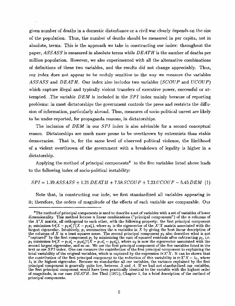
given number of deaths in a domestic disturbance or a civil war clearly depends on the size

of the population. Thus, the number of deaths should be measured in per capita, not in

absolute, terms. This is the approach we take in constructing our index: throughout the

paper, ASS ASS is measured in absolute terms while DEATH is the number of deaths per

million population. However, we also experimented with all the alternative combinations

of definitions of these two variables, and the results did not change appreciably. Thus,

our index does not appear to be unduly sensitive to the way we measure the variables

ASS ASS and DEATH. Our index also includes two variables (SCOUP and UCOUP)

which capture illegal and typically violent transfers of executive power, successful or at-

tempted. .The variable DEM is included in the SPI index mainly because of reporting

problems: in most dictatorships the government controls the press and restricts the diffu-

sion of information, particularly abroad. Thus, measures of socio-political unrest are likely

to be under-reported, for propaganda reasons, in dictatorships.

The inclusion of DEM in our SPI index is also advisable for a second conceptual

reason. Dictatorships are much more prone to be overthrown by extremists than stable

democracies. That is, for the same level of observed political violence, the likelihood

of a violent overthrown of the government with a breakdown of legality is higher in a

dictatorship.

Applying the method of principal components8 to the five variables listed above leads

to the following index of socio-political instability:

SPI = 1.39 ASS ASS + 1.21 DEATH + 7.58 SCOUP + 7.23 UCOUP - 5.45 DEM (1)

Note that, in constructing our inde, we first standardized all variables appearing in

it; therefore, the orders of magnitude of the effects of each variable are comparable. Our

8The method of principal components is used to describe a set of variables with a set of variables of lowerdimensionality. This method locates n linear combinations ("principal components") of the n columns ofthe X'X matrix, all orthogonal to each other, with the following property: the first principal componentPi minimizes tr(X — p\a'i)'(X — pia[), where a\ is the eigenvector of the X'X matrix associated with thelargest eigenvalue. Intuitively, p\ summarizes the n variables in X by giving the best linear description ofthe columns of X in a least squares sense. The second principal component p2 also describes what is not"captured" by the first component p\ by minimizing the sum of squared residuals after subtracting pi, i.e.P2 minimizes tr(X — p\a'x — p2a'2y(X — pia'j — P2<*2)> w n e r e a2 is n o w the eigenvector associated with thesecond largest eigenvalue, and so on. We use the first principal component of the five variables listed in thetext as our SPI index. One can measure the contribution of the first principal component to explaining thetotal variability of the original variables, which is captured by the expression trX'X. It can be shown thatthe contribution of the first principal component to the reduction of this variability is trX'X — Ai, whereAi is the highest eigenvalue. Because we standardize all our variables, the variance explained by the firstprincipal component is generally quite low, between .3 and .4. If we had not standardized our variables,the first principal component would have been practically identical to the variable with the highest orderof magnitude, in our case DEATH. See Theil (1971), Chapter 1, for a brief description of the method ofprincipal components.

SPI index is related, but far from identical, to indices recently proposed by Venieris and

Gupta (1986) and Gupta (1990), which we used in previous versions of this paper, and

is somewhat different from Hibbs' (1973) index. Section 6 discusses the robustness of our

results to the use of these alternative indices and to small changes in the specification of

our index.

3 Data and sample period.

We perform cross sectional regressions using a sample of 71 countries for the period 1960-

1985. The binding constraint on the number of countries is the data availability. We

have income distribution data for 74 countries, but for only 71 of these we have data on

political instability and the other variables we use in our regressions, like investment shares

in 1960-85 and GDP per capita in 1960.

We use the same dataset on income distribution assembled by Perotti (1994). The in-

come distribution data consist of the income shares of the five quintiles of the population,

measured as close as possible to the beginning of each sample period, 1960. In our frame-

work, income distribution is predetermined; therefore, it is appropriate to measure this

variable at the beginning of the sample period. In fact, in the long run income distribution

is likely to be endogenous, as it is arguably affected by such factors as land reforms, the

savings behavior of the population etc. These problems of endogeneity are clearly hard to

overcome: however, measuring income distribution at the beginning of the sample period

is a way of minimizing them.

Data on quintiles shares in existing datasets on income distribution derive from surveys

conducted at different times, and differ in terms of their coverage (nationwide, urban,

etc.), of the definition of income (pre-tax, pre-transfers, etc.), and of the definition of

recipient unit (by households, by economically active persons, by individuals, etc.). In

principle, all data refer to pre-tax income, while transfers are generally (but not always)

included in data organized by households but not in data by economically active persons or

individulas. However, in the surveys the actual definition of income used by the respondent

is very difficult to control, particularly in developing countries. Since income distribution

data generally come from expenditure surveys, it is likely that in most cases transfers are

included in the responses used to construct the income shares.

The majority of countries in our sample have data by households with nationwide cov-

erage. For the remaining countries, observations organized by economically active persons

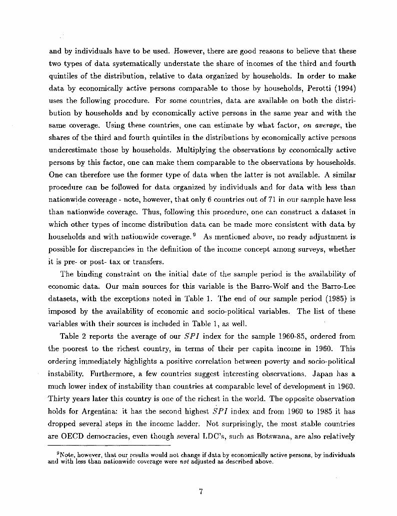
and by individuals have to be used. However, there are good reasons to believe that these

two types of data systematically understate the share of incomes of the third and fourth

quintiles of the distribution, relative to data organized by households. In order to make

data by economically active persons comparable to those by households, Perotti (1994)

uses the following procedure. For some countries, data are available on both the distri-

bution by households and by economically active persons in the same year and with the

same coverage. Using these countries, one can estimate by what factor, on average, the

shares of the third and fourth quintiles in the distributions by economically active persons

underestimate those by households. Multiplying the observations by economically active

persons by this factor, one can make them comparable to the observations by households.

One can therefore use the former type of data when the latter is not available. A similar

procedure can be followed for data organized by individuals and for data with less than

nationwide coverage - note, however, that only 6 countries out of 71 in our sample have less

than nationwide coverage. Thus, following this procedure, one can construct a dataset in

which other types of income distribution data can be made more consistent with data by

households and with nationwide coverage.9 As mentioned above, no ready adjustment is

possible for discrepancies in the definition of the income concept among surveys, whether

it is pre- or post- tax or transfers.

The binding constraint on the initial date of the sample period is the availability of

economic data. Our main sources for this variable is the Barro-Wolf and the Barro-Lee

datasets, with the exceptions noted in Table 1. The end of our sample period (1985) is

imposed by the availability of economic and socio-political variables. The list of these

variables with their sources is included in Table 1, as well.

Table 2 reports the average of our SPI index for the sample 1960-85, ordered from

the poorest to the richest country, in terms of their per capita income in 1960. This

ordering immediately highlights a positive correlation between poverty and socio-political

instability. Furthermore, a few countries suggest interesting observations. Japan has a

much lower index of instability than countries at comparable level of development in 1960.

Thirty years later this country is one of the richest in the world. The opposite observation

holds for Argentina: it has the second highest SPI index and from 1960 to 1985 it has

dropped several steps in the income ladder. Not surprisingly, the most stable countries

are OECD democracies, even though several LDC's, such as Botswana, are also relatively

9Note, however, that our results would not change if data by economically active persons, by individualsand with less than nationwide coverage were not adjusted as described above.

stable. The case of Venezuela is also interesting: in 1960 it had the fifth highest per capita

income in the sample, but a much higher SPI index than the countries in the same group.

Table 3 reports the summary statistics for our variables and Table 4 highlights simple

correlations between them. The two key correlations for our purposes are those between

SPI and investment, INV', and between SPI and MIDCLASS, which represents the

share of total income of the third and fourth quintiles of the population.

The two correlations are -.42 and -.47, respectively. These signs are consistent with

our hypothesis, namely that socio-political instability depresses investment and income

inequality makes the socio-political environment more unstable. Also, SPI is negatively

correlated with both the level of income and the level of education. However, the latter two

variables are highly correlated with each other. Note that MI DC LASS has a much higher

correlation with secondary school enrollment than with primary school enrollment. This

correlation suggests, perhaps, that if the middle class is sufficiently well off, they can obtain

for their children a level of education beyond the primary one. Because of this correlation,

and because our sample includes several LDC's in which enrollment ratios in secondary

schools in 1960 were extremely small, we prefer to use primary school enrollment as our

measure of education. Finally, in our sample MIDCLASS has a correlation of -.93 with

the share of the richest quintile (not shown). This implies that an increase in the share

of the middle class is associated, on average, with essentially a one for one decrease in the

share of the richest quintile. This is the main reason why the two variables do not appear

at the same time in our regressions.

Also, Table 4 reports the correlations of our index with its components. Using these

correlations with the coefficients of the SPI index displayed in eq. (1), one can form an

idea of the importance of each component in our results. We discuss this topic extensively

in section 6.

4 Model specification.

Our hypothesis is that income inequality increases socio-political instability and the latter

reduces the propensity to invest. A large group of impoverished citizens, facing a small

and very rich group of well-off individuals is likely to become dissatisfied with the existing

socio-economic status quo and demand radical changes, so that mass violence and illegal

seizure of power are more likely than when income distribution is more equitable. Several

arguments justify the second link, from political instability to investment. Broadly speak-

ing, political instability affects investment through three main channels. First, because it

increases the expected level of taxation of factors that can be accumulated, through the

mechanism noted in section 2. Second, because phenomena of social unrest can cause dis-

ruption of productive activities, and therefore a fall in the productivity of labor and capital.

Third, because socio-political instability increases uncertainty, thereby inducing investors

to postpone projects, invest abroad (capital flights) or simply consume more. In turn, a

high value of the SPI index implies high uncertainty for two reasons. First, when social

unrest is widespread, the probability of the government being overthrown is higher, making

the course of future economic policy and even protection of property rights more uncertain.

Second, the occurrence of attempted or successful coups indicates a propensity to abandon

the rule of law and therefore, in principle, a threat to established property rights.

We capture these two links in a simple bivariate simultaneous equation model with SPI

and investment as endogenous variables. The most basic specification of this model is as

follows:

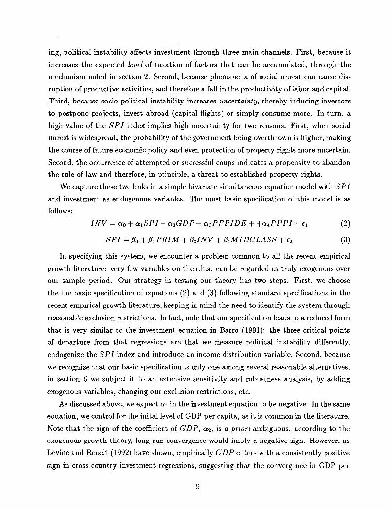
INV = a0 + OLXSPI + a2GDP + azPPPIDE + +aAPPPI + Cl (2)

SPI = p0 + ft PRIM + (33INV + /34MIDCLASS + e2 (3)

In specifying this system, we encounter a problem common to all the recent empirical

growth literature: very few variables on the r.h.s. can be regarded as truly exogenous over

our sample period. Our strategy in testing our theory has two steps. First, we choose

the the basic specification of equations (2) and (3) following standard specifications in the

recent empirical growth literature, keeping in mind the need to identify the system through

reasonable exclusion restrictions. In fact, note that our specification leads to a reduced form

that is very similar to the investment equation in Barro (1991): the three critical points

of departure from that regressions are that we measure political instability differently,

endogenize the SPI index and introduce an income distribution variable. Second, because

we recognize that our basic specification is only one among several reasonable alternatives,

in section 6 we subject it to an extensive sensitivity and robustness analysis, by adding

exogenous variables, changing our exclusion restrictions, etc.

As discussed above, we expect a\ in the investment equation to be negative. In the same

equation, we control for the inital level of GDP per capita, as it is common in the literature.

Note that the sign of the coefficient of GDP, a.2-, is a priori ambiguous: according to the

exogenous growth theory, long-run convergence would imply a negative sign. However, as

Levine and Renelt (1992) have shown, empirically GDP enters with a consistently positive

sign in cross-country investment regressions, suggesting that the convergence in GDP per

9

capita occurs through channels different from increases in physical investment. The two

variables PPPI (the PPP value of the investment deflator in 1960 relative to that of

the U.S.) and PPPIDE (the magnitude of the deviation of PPPI from the sample mean)

capture the effects of domestic distortions which obviously would affect investment directly.

Turning to the SPI equation, we included the variable PRIM (the enrollment ratio in

primary school in 1960) as a proxy for human capital, on the ground that a higher level

of education may reduce political violence and channel political action within institutional

rules (see Huntington (1968) or Hibbs (1973)).10 Therefore, we expect /?x to be negative.

Investment is also included to test whether rapidly growing economies tend to be more

stable: on the one hand, more growth means more prosperity, less dissatisfaction and

possibly more stability, implying a negative sign for /?2. On the other hand, periods of

very high growth may temporarily lead to social disruptions and economic transformation

which may actually increase political instability. Finally, as discussed at length above, we

expect a positive relation between inequality and instability: accordingly, under the null

hypothesis the sign of /?3 should be negative when an index of equality is used.

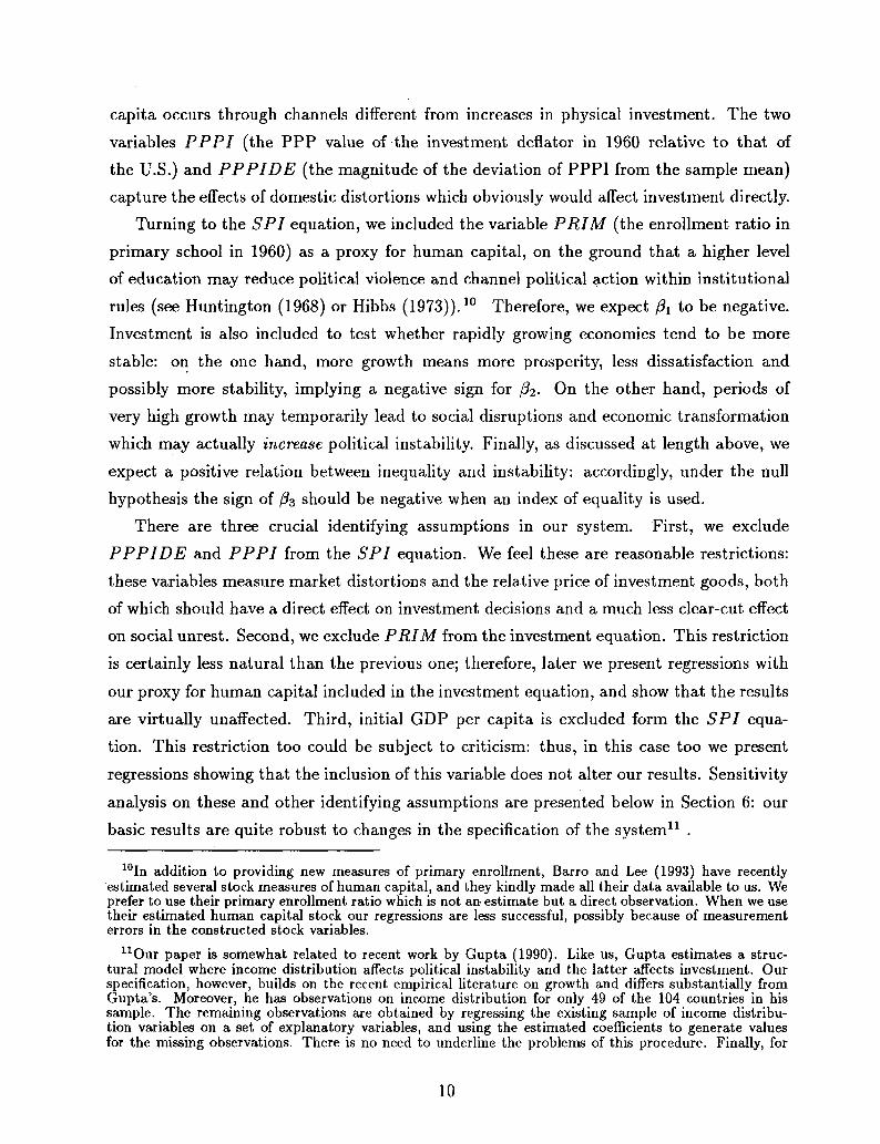
There are three crucial identifying assumptions in our system. First, we exclude

PPPIDE and PPPI from the SPI equation. We feel these are reasonable restrictions:

these variables measure market distortions and the relative price of investment goods, both

of which should have a direct effect on investment decisions and a much less clear-cut effect

on social unrest. Second, we exclude PRIM from the investment equation. This restriction

is certainly less natural than the previous one; therefore, later we present regressions with

our proxy for human capital included in the investment equation, and show that the results

are virtually unaffected. Third, initial GDP per capita is excluded form the SPI equa-

tion. This restriction too could be subject to criticism: thus, in this case too we present

regressions showing that the inclusion of this variable does not alter our results. Sensitivity

analysis on these and other identifying assumptions are presented below in Section 6: our

basic results are quite robust to changes in the specification of the system11 .

10In addition to providing new measures of primary enrollment, Barro and Lee (1993) have recentlyestimated several stock measures of human capital, and they kindly made all their data available to us. Weprefer to use their primary enrollment ratio which is not an estimate but a direct observation. When we usetheir estimated human capital stock our regressions are less successful, possibly because of measurementerrors in the constructed stock variables.

nOur paper is somewhat related to recent work by Gupta (1990). Like us, Gupta estimates a struc-tural model where income distribution affects political instability and the latter affects investment. Ourspecification, however, builds on the recent empirical literature on growth and differs substantially fromGupta's. Moreover, he has observations on income distribution for only 49 of the 104 countries in hissample. The remaining observations are obtained by regressing the existing sample of income distribu-tion variables on a set of explanatory variables, and using the estimated coefficients to generate valuesfor the missing observations. There is no need to underline the problems of this procedure. Finally, for

10

We have also built upon this basic specification by adding other exogenous variables.

We added in the SPI equation a variable that captures the degree of linguistic and ethnic

fragmentation, on the ground that more homogeneous societies are likely to exhibit, ceteris

paribus, less socio-political instability. We also included a variable for urbanization in

the SPI equation: several political scientists (for instance, Huntington (1968) and Hibbs

(1973)) have argued that more urbanized societies should be more politically unstable

because political participation and social unrest are more likely to be higher in cities.

Finally, one could argue that income distribution can affect investment directly, not only

through political instability, but also through two additional channels. The first one is a

"Kaldorian" saving function. According to Kaldor (1956), the "capitalists" save more in

proportion to their income than the "workers". Testing this hypothesis would require data

on the functional distribution on income, which is not available for most countries in our

sample. However, since income from capital is typically concentrated in the top quintile

of the population, there is a strong correlation between functional distribution of income

and the share of income of the top quintile or of the middle class. Thus, the "Kaldorian"

hypothesis could be expressed as a negative relationship between the share of the middle

class and the saving rate and therefore investment, after controlling for the effects of income

distribution on investment through its effects on socio-political instability. On the other

hand, Alesina and Rodrik (1994) and Bertola (1994) argue that the more unequal the

distribution of income, the higher is the demand for fiscal redistribution through taxation

of capital. The latter may depress investment by increasing the tax burden on investors.

In order to explore these direct channel we have run a second specification, in which we

added an income distribution variable in the investment equation. However, since the two

channels discussed above go in opposite direction, the sign of the associated coefficient is a

priori ambiguous.

Finally, note that the dependent variable in equation (2) is total investment (INV).

We use total rather than private investment because the breakdown of investment between

private and public is available only for 56 of the 71 countries of our sample and only from

1970 onward. Aside from considerations of data availability, there are reasons to believe

that public investment as well as private investment should be negatively affected in periods

of high socio- political instability. Since these are usually periods of high and contrasting

reasons that are not clear to us, in all his regressions Gupta uses the 1970 value of the SPI index ratherthan its average on the estimation period as we do. These and other differences are sufficient to explainthe difference in results between the two works: in fact, contrary to our results, in Gupta's book bothincome distribution and political instability turn out to be insignificant in explaining political instabilityand investment respectively.

11

demands on the government budget, public investment projects are likely to be reduced to

make room for redistributive expenditure.

5 Estimation of the basic specification.

We start by estimating the basic specification of equations (2) and (3) in columns (la)

and (lb) of Table 5. The two key coefficients are those that capture the effects of SPI

on INV and of MIDCLASS on SPI. Both coefficients have the expected signs and are

significant at the 5% level: socio-political instability depresses investment and a rich middle

class reduces socio-political instability. A "healthy" middle class is conducive to capital

accumulation because it creates conditions of social stability. As noted above, the share

of income of the middle class has a correlation of almost -1 with the share of the richest

quintile; thus, a wealthier middle class implies more equality in the distribution of income.

An increase by one standard deviation of the share of the middle class is associated with

a decrease in the index of political instability by about 5.7, which corresponds to about

48% of its standard deviation. This in turn is associated with an increase in the share

of investment in GDP of about 2.85 percentage points. The effect of income distribution

on investment implied by these estimates is definitely not negligible, since the difference

between the highest and lowest value of MIDCLASS in the sample is about 4 standard

deviations. In addition, an exogenous increase in the SPI index by one standard deviation

causes a decrease in the share of investment in GDP of about 5.97 percentage points.

The coefficient on PPPI in the investment equation has the expected negative sign

and is significant at high levels of confidence: market distortions do have negative effects

on investment. The second proxy for market distortions, PPPIDE, is insignificant. Con-

sistently with the results of the existing literature, initial GDP per capita has a positive,

although insignificant, coefficient.12

The estimation results for the SPI equation are also very sensible. PRIM has a

negative and significant coefficient: as expected, countries with higher levels of education

tend to be more stable.

In columns (2a) and (2b) we add three regional dummies, ASIA (for the East Asian

countries), LA AM (for Latina American countries) and AFRICA (for Sub-Saharan coun-

tries), in the SPI equation. There are at least two reasons for this: first, cultural and/or

12Note that our results in the investment equation are consistent with the reduced form results in Barro(1991).

12

historical reasons may influence the amount of socio-political unrest in different regions of

the world. Second, in certain regions., particularly Africa, under-reporting of socio-political

events can be particularly acute. Of the three regional dummies, only LA AM is significant:

as expected, on average Latin American countries tend to be much more unstable than the

other countries in the sample. The coefficient of SPI in the investment equation is very

similar to that of column (la), while the coefficient of MIDCLASS in the SPI equation

drops (in absolute value) by about 30% to -.68, although it remains strongly significant.

This is hardly surprising, since the Latin America countries in the sample are more unstable

than the average and, especially, have a particularly unequal distribution of income. Since

regional dummies do appear to be important in our regressions, from now on we include

them in all our reported estimates; it might be worthwhile noting that, if we did not include

them, in general our results on the income distribution variable would be stronger than the

ones we report.13

6 Robustness and sensitivity analysis.

We first tested the sensitivity of our results to the particular SPI index used. In a previ-

ous version of this paper we used an index proposed by Gupta (1990): this index (SPIG)

was obtained by applying the method of discriminant analysis to a larger sample than

ours (about 100 countries). In addition to the variables used in our index14 , Gupta in-

cludes: PROTEST, the number of political demonstrations against a government; RIOT,

the number of riots; STRIKE, the number of political strikes; ATTACK, the number

of politically motivated attacks; EXECUTION, the number of politically motivated ex-

ecutions. Thus, our index differs from Gupta's for three reasons: his sample of countries

is different, he uses discriminant analysis rather than the principal component method to

construct it, and he includes many more variables. Despite these differences, the correlation

13As mentioned above, the breakdown of total investment into private and public investment is availableonly for 56 countries and only from 1970 onward. We estimated the same specifications of Table 5 usingthe average rate of private investment in the 1970-85 period with the following results: the effect of SPI oninvestment remains large and statistically significant; the coefficient of MIDCLASS in the SPI equationhas the correct sign but is not significant at conventional-levels. We repeated the same regressions usingtotal investment over the same sample 1970-85: the results were essentially identical to those obtained whenusing private investment. These findings (available upon request) suggest that the difference between theresults of Table 5 and those obtained with private investment are due to the sample size but especiallyto the shorter time period. A fifteen year period (1970-85) may be too short for the type of structural,long-run relationship between inequality and instability that we are testing. Therefore, we feel that it ismore reasonable to place more weight on the results obtained for the 1960-85 period.

14Note however that Gupta's measure of the variable DEM is slightly different from ours, although thetwo measures are highly correlated.

13

of Gupta's index to ours is extremely high, about .83 (see Table 4). Table 6 reports the

results obtained when using Gupta's SPIG index in the same systems estimated in Table

5.

Both the coefficient of the SPIG index in the investment equation and of MIDCLASS

in the SPIG equation have the expected sign and are significant at conventional levels.

Interestingly, the size of the coefficients in columns (la) and (lb) of Table 6 are such that

an increase in MIDCLASS by one standard deviation has similar effects on SPIG and,

through the latter, on investment as in the corresponding regressions of columns (la) and

(lb) of Table 5, where our SPI index is used. All the other coefficients too exhibit patterns

very similar to those of Table 5.

We have experimented by applying the principal component method to several combi-

nations of the long list of variables included in the Gupta's index. The pattern of results

that we obtain (available upon request) can be summarized as follows. First, when we

add RIOT, PROTEST, ATTACK or EXECUTION to the list of variables of our SPI

index, the results remain largely unaffected, and in some cases are even stronger than those

we have presented. The results are also largely independent of whether we use per capita or

total values for the variables that can be interpreted both ways, like the number of assassi-

nations, deaths, attacks, executions etc. Our results worsen slightly, compared to those of

Table 5, with indices that do not include successful and unsuccessful coups. This finding

suggests that these two variables are important to capture threats to property rights and

policy uncertainty. Finally, if we leave out the variable DEM, our results generally worsen.

Table 7 displays several additional specifications that build upon the basic one. In

this table we use our SPI index, but the results (available upon request) are very similar

when the SPIG index is used. Also, because we include the regional dummies in the SPI

equation, the estimates that appear in these two tables should be compared to columns

(2a) and (2b) of Table 5.

First, as discussed in section 4, there might be good reasons to include PRIM in the

investment equation, on the ground that physical and human capital might be complemen-

tary. Also, it might be important to control for GDP in the SPI equation, to test the

notion that "good things tend to go together", so that richer countries are more stable.

Columns (la) and (lb) of Table 7 control for PRIM in the investment equation and for

GDP in the SPI equation, respectively. The coefficients of both variables have the ex-

pected signs, although only PRIM in the investment equation is significant. Importantly,

the coefficients of SPI in the investment equation and of MIDCLASS in the SPI equation

14

remain significant and largely unaffected relative to columns (2a) and (2b) of Table 5. The

coefficient of SPI falls in absolute value, from -.57 to -.40: this too is not surprising, since

primary school enrollment has a large negative correlation with socio-political instability.

In columns (2a) and (2b) of Table 7 we add the variable HOMOG in the SPI equation.

This variable is defined as the fraction of the population (in 1960) belonging to the main

ethnic and linguistic group. Thus, a lower value of this variable implies more ethnic frag-

mentation, which is likely to be a cause of political instability and mass violence (Hibbs

(1973)). The coefficient on this variable has the expected sign but is not significant at

conventional levels. Generally, depending on the other variables included in the regression,

HOMOG ha,s a coefficient which is always negative (as expected) but with varying degrees

of statistical significance. The estimates of the remaining coefficients are very similar to

those of columns (2a) and (2b) in Table 5.

Columns (3a) and (3b) of Table 7 display the estimate of the system with an income

distribution variable appearing directly in the investment equation. The rationale for this

specification follows directly from the arguments briefly surveyed in section 4. The coeffi-

cient on MIDCLASS in the investment equation is negative, suggesting that a "Kaldorian"

link between income distribution and investment is at work: economies with less concen-

trated distributions of income save and invest less. However, note that the coefficient is

statistically insignificant; moreover, as we discussed in section 4 the proper way to test the

Kaldorian hypothesis would be to use measures of the functional distribution of income,

which unfortunately is not available for most of the countries of our sample. We also es-

timated the same system, with the share of the bottom two quintiles of the population or

the share of the top quintile as the income distribution variable instead of MIDCLASS

in the investment equation. In both cases, the coefficient of the income distribution vari-

able is close to 0, and insignificant. These results have two possible interpretations. The

first one is that the only effect of income inequality on capital accumulation goes through

political instability. The second one is that, once political instability is controlled for, the

"Kaldorian" effect and the fiscal redistribution effect offset each other.

We also added several other exogenous variables that, on a priori grounds, are po-

tentially important determinants of investment and socio-political instability. In general,

none of these variables changed our results concerning the effects of income distribution

on socio-political instability and of the latter on investment. Two of these variables ap-

pear particularly interesting: urbanization and government consumption. As argued by

Huntington (1968) and Berg and Sachs (1988), urbanization leads to more social demands

15

and political pressure for redistributive policies. Indeed, when we include a measure of

urbanization in 1960 among the regressors of the SPI equation, its coefficient is positive,

but insignificant. To the extent that government consumption is a proxy for the size of

government and government-induced distortions, one can argue that it should have a neg-

ative effect on investment. On the other hand, government consumption might belong in

the SPI equation, as higher expenditure by the government might be used to prevent or

defuse social unrest. We tried both specifications: indeed, government consumption has

a negative coefficient in both the investment and the SPI equation, although only in the

latter it is close to being significant. Importantly, both when urbanization and government

consumption are controlled for, the coefficients of SPI in the investment equation and of

MI DC LASS in the SPI equation are virtually unaffected.

We tried several additional permutations in the specification, using the two indices

of political instability and various combinations of the variables discussed so far. Our

results (available upon request) confirm the robustness of our findings both on the effects

of inequality on political instability and on the effects of the latter on investment.

We did find, however, an interesting exception, which we show in columns (4a) and (4b)

of Table 7: our results worsen significantly when we use the enrollment ratio in secondary

school (SEC), rather than in primary school, to control for human capital. In particular,

the coefficient of SPI in the investment equation falls only slightly in absolute value,

and remains strongly significant; but the coefficient of MI DC LASS in the investment

equation falls substantially, to -.38, and becomes insignificant. These results are due to the

high degree of correlation between SEC and MIDCLASS, which is about .6, i.e. roughly

double that between PRIM and MIDCLASS (see Table 4). Because of this pattern of

correlations, it becomes hard to disentangle the effects of income distribution on secondary

school enrollment and on SPI separately, while the problem is less acute when we use

instead primary school enrollment.

The high correlation between secondary school enrollment and MIDCLASS suggests

an additional channel through which income equality may enhance growth and accumula-

tion: in the presence of liquidity constraints due to capital market imperfections, a wealthy

middle class can afford to invest in higher education, while an impoverished one cannot. A

more extensive empirical analysis of the relationship between inequality and investment in

education is left for further research.15

An additional way of looking at the robustness of the results is to estimate the model

15See Perotti (1993) and Fernandez and Rogerson (1991) for theoretical discussions of this issue.

16

using robust estimation methods. Roughly speaking, robust regression methods provide

estimators that downweigh those observations that are "outliers". One dimension along

which the robust estimators differ is the definition of an "outlier". Typically, an outlier is

characterized by a large residual. We have chosen to estimate the SPI and INV equations

by applying the bounded-influence estimator proposed by Krasker and Welsch (1982). The

main reason for this choice is that this estimator identifies and downweighs outliers not only

in the residuals' space, but also in the regressors' space. As shown by Krasker and Welsch

(1983), an observation can be very influential and nevertheless the residual corresponding

to that observation may be smaller than most other residuals. Since we are estimating a

simultaneous-equation model, we implement the 2SLS version of the Krasker and Welsch

estimator.16

Table 8 shows the Krasker and Welsch estimates of one of the basic specifications

of the SPI and INV equations, both with our index of socio-political instability and

with Gupta's. Thus, columns (la) and (lb) of Table 8 present the 2SLS Krasker-Welsch

estimates of columns (2a) and (2b) in Table 5, while columns (2a) and (2b) present the

2SLS Krasker-Welsch estimates of the columns (2a) and (2b) in Table 6. One can see

immediately that the point estimates of virtually all the coefficients are very similar, and

in many cases almost identical, to those of the 2SLS estimators. The main exception is the

coefficient of MIDCLASS in column (lb), which is -.49, against -.68 in column (2b) of

Table 5. Given the well known problems with measuring income distribution from surveys,

it is not entirely surprising that the coefficient of MIDCLASS should be less robust than

the others coefficients in our regressions; however, this coefficient remains significant even

in the robust regression.

The relative efficiency of the Krasker-Welsch estimator is always below .95, which is

often the value used in applied work. This is an indication that the estimates are indeed

robust: the less efficient is the Krasker-Welsch estimator relative to the 2SLS estimator,

the easier it is for an observation to be considered an outlier. 17 These results are

quite reassuring: although there are well known measurement error problems in income

distribution and political data, they are not of such a nature as to make the estimates of

16Robust estimator for 3SLS have not been devised yet. See Krasker and Welsch (1982) and Krasker,Kuhand Welsch (1983) for a theoretical treatment of robust estimators, and Kuh and Welsch (1980) and Peters,Samarov and Welsch (1982) for some applications. The estimates of this section are obtained by applyinga RATS program implemented in Perotti (1994).

17The reason why relative efficiencies are different in different equations is that we fixed the constant cin Peters, Samarov and Welsch (1982) at a value of .55 rather than adjusting it every time to achieve adesired value of relative efficiency.

17

the model very sensitive to some particular observation.

Finally, we addressed the related issues of heteroskedasticity and misspecification due

to measurement errors. We therefore conducted several tests of misspecification and het-

eroskedasticity on the same systems that appear in Table 5. A first rough indicator of the

presence of misspecification possibly due to errors-in-variables problems is provided by a

Hausman test using 2SLS and 3SLS estimates. The statistic was never significant at the

10% level. As to heteroskedasticity, we ran a Breusch-Pagan test on the SPI equation,

assuming that the error variance was proportional to the inverse of initial GDP.18 Again,

the test was never significant. As an additional check, we reestimated the SPI equa-

tion applying White's heteroskedasticity correction, which in this IV framework becomes

White's Two-Stage-Instrumental-Variables estimator (see White (1983)). Again, neither

the coefficient estimates nor the t-statistics changed substantially.

7 Conclusions.

Income inequality increases socio-political instability which in turn decreases investment.

After an extensive battery of robustness tests, we can conclude that these results in our

sample of 71 countries are quite solid.

These results have positive and normative implications. From a positive point of view

they suggest an argument that might help explain different investment and growth perfor-

mances in different parts of the world. Several countries in South East Asia have had very

high growth rates in the post-WWII period. In the aftermath of the war, these countries

had land reforms that reduced income and wealth inequality. Furthermore, and, perhaps as

a result of this reform, these countries have been relatively stable politically, compared to,

say, Latin American countries. The latter, in turn, have had a much more unequal income

distribution, more socio-political instability and less growth. A particularly good example

of successful Asian countries are the "four dragons" (Hong Kong, Singapore, South Korea,

and Taiwan). Unfortunately, because of data availability, these countries are not included

in our regressions. However, they would seem to fit our hypothesis, since these countries

have had much more stability and much less inequality than, say, Latin American countries,

which had a comparable GDP per capita in 1960.

From a normative point of view, our results have some implications for the effects of

18If errors in measuring income distribution are more severe in poorer countries, for instance becausethe surveys are conducted with smaller budgets, the induced error variance will be inversely proportionalto GDP.

18

redistributive policies. Fiscal redistribution, by increasing the tax burden on capitalists and

investors, reduces the propensity to invest. However, the same policies may reduce social

tensions and, as a result, create a socio-political climate more conducive to productive

activities and capital accumulation. 19 Thus, by this channel fiscal redistribution might

actually spur economic growth. Therefore the net effect of redistributive policies on growth

has to weigh the costs of distortionary taxation against the benefits of reduced social

tensions.

This paper, not unlike the related literature surveyed in the introduction, focuses on

policy outcomes (investment, growth etc.) and relates them to socio-economic variables.

The next step in this line of research is to look more explicitly at actual policy instruments,

as Perotti (1994) has started doing. The link between politics and economic outcomes goes

through policy choices, particularly, in this context, fiscal policy. Several questions are left

open: what are the effects of income inequality on the degree of redistribution implemented

in different political systems? Who actually benefits from such redistributions? What

are the distributional effects of different spending programs? Do the very poor really

benefit from government programs toward them? Answering these questions requires more

disaggregated fiscal policy data than those used so far.

19A similar argument has been put forward by Sala y Martin (1992). A related argument, suggestedby Fay (1993), focuses on illegal activities. Higher inequality fuels crime against private property; thusredistributive policies protect property rights by reducing crime.

19

Table 1: Definition of variables and data sources.

This Table describes the data used in the regressions. All the data are from the Barro-Wolf

[1990] data set, except for the income distribution data which are mainly from Jain (1975)

(see Perotti (1994) for a more detailed list of the original sources) or unless otherwise in-

dicated.

GDP: GDP in 1960 in hundreds of 1980 dollars;

PRIM: primary school enrollment rate in 1960, from Barro and Lee (1993);

SEC: secondary school enrollment rate in 1960, from Barro and Lee (1993);

MI DC LASS: share of the third and fourth quintiles of the population in or around 1960;

INV: ratio of real domestic investment (private plus public) to real GDP (average from

1960 to 1985);

PPPI: PPP value of the investment deflator (U.S. = 1.0), 1960;

PPP IDE: Magnitude of the deviation of the PPP value for the investment deflator from

the sample mean, 1960;

SPI: index of socio-political instability, constructed using averages over 1960-85 of the

variables that appear in the formula of equation (1);

SPIG: index of socio-political instability, constructed using annual data from the formula

in Gupta (1990), average over 1960-85;

HOMOG: percentage of the population belonging to the main ethnic or linguistic group,

1960, from Canning and Fay (1993);

URB: Urban population as percentage of total in 1960. Source: World Bank Tables;

GOV: Government consumption as share of GDP, average 1970-85;

DEATH: average number of deaths in domestic disturbances, per millions population,

1960-85, from Jodice and Taylor (1988);

ASS ASS: average number of assassinations, 1960-85, from Jodice and Taylor (1988);

UCOUP: average number of unsuccessful coups, 1960-85, from Jodice and Taylor (1988);

SCOUP: average number of successful coups, 1960-85, from Jodice and Taylor (1988);

DEM: Dummy variable taking the value 1 for democracies, .5 for semi-democracies, and

0 for dictatorships, average 1960-85, from Jodice and Taylor (1988).

20

Table 2: SPI index (sample 1960-85).

COUNTRY SPI COUNTRY SPI

TanzaniaMalawiSierra LeoneNigerBurmaTogoBangladeshKeniaBotsawanaEgyptChadIndiaMoroccoNigeriaPakistanCongoBeninZimbabweMadagascarSudanThailandZambiaIvory CoastHondurasSenegalGabonTunisiaPhilippinesBoliviaDom. RepublicSri LankaEl SalvadorMalaysiaEcuadorTurkey

-.73-2.669.113.421.586.808.39-.72

-9.681.837.61

-8.922.41

12.699.11

21.6630.34-1.762.42

15.099.31

-3.46-2.745.00-.984.05

-2.57-4.1444.19

8.22-9.917.94

-11.2119.912.88

PanamaBrazilColombiaJamaicaGreeceCostaricaCyprusPeruBarbadosIranMexicoJapanSpainIraqIrelandSouth AfricaIsraelChileArgentinaItalyUruguayAustriaFinlandFranceHollandU.K.NorwaySwedenAustraliaGermanyVenezuelaDenmarkNew ZealandCanadaSwitzerlandU.S.A.

5.42-.19

-4.69-11.60

2.41-11.76-5.557.46

-11.76-1.13-4.15

-11.68-2.7730.64

-11.37-7.08

-11.67.50

30.54-8.104.80

-11.68-11.76-9.44

-11.68-7.63

-11.76-11.68-11.68-11.45

4.03-11.76-11.76-11.68-11.76-11.06

21

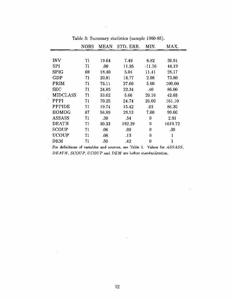
Table 3: Summary statistics (sample 1960-85).

NOBS MEAN STD. ERR. MIN. MAX.

INVSPISPIGGDPPRIMSECMIDCLASSPPPIPPPIDEHOMOGASSASSDEATHSCOUPUCOUPDEM

717169717171717171677171717171

19.64.00

18.4020.8176.1124.8533.6270.2519.7458.89

.3030.33

.06

.08

.50

7.4911.955.0418.7727.6022.345.66

24.7415.4229.53

.54192.29

.09

.13

.42

6.82-11.7611.412.085.00.40

20.1026.00

.037.00

00000

36.9144.1928.1773.80

100.0086.0042.03161.1086.3099.002.91

1619.72.3911

For definitions of variables and sources, see Table 1. Values for ASSASS,

DEATH, SCOUP, UCOUP and DEM are before standardization.

22

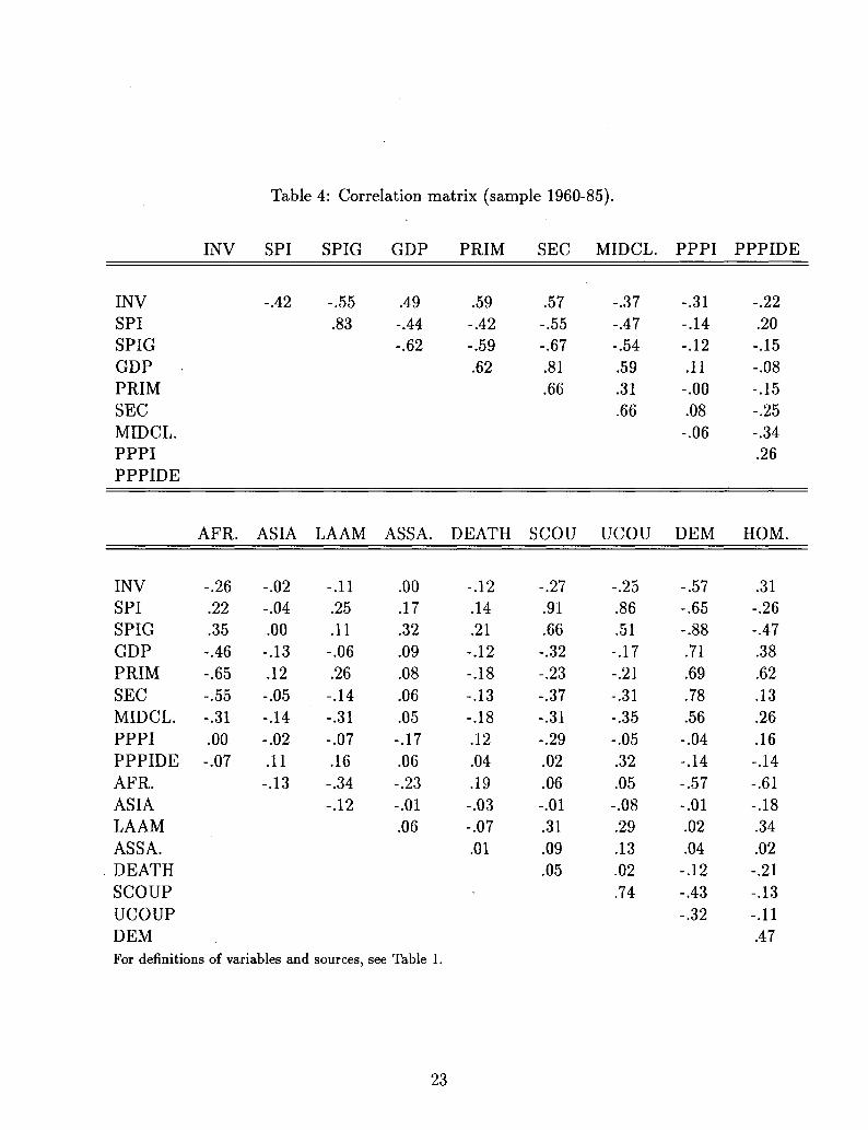
Table 4: Correlation matrix (sample 1960-85).

INV SPI SPIG GDP PRIM SEC MIDCL. PPPI PPPIDE

INVSPISPIGGDPPRIMSECMIDCL.PPPIPPPIDE

INVSPISPIGGDPPRIMSECMIDCL.PPPIPPPIDEAFR.ASIALAAMASSA.DEATHSCOUPUCOUPDEM

AFR.

-.26.22.35-.46-.65-.55-.31.00-.07

-.42

ASIA

-.02-.04.00-.13.12-.05-.14-.02.11-.13

-.55.83

LAAM

-.11.25.11-.06.26

-.14-.31-.07.16

-.34-.12

.49-.44-.62

ASSA.

.00

.17

.32

.09

.08

.06

.05-.17.06-.23-.01.06

.59-.42-.59.62

DEATH

-.12.14.21

-.12-.18-.13-.18.12.04.19-.03-.07.01

.57-.55-.67.81.66

SCOU

-.27.91.66-.32-.23-.37-.31-.29.02.06-.01.31.09.05

-.37-.47-.54.59.31.66

UCOU

-.25.86.51-.17-.21-.31-.35-.05.32.05-.08.29.13.02.74

-.31-.14-.12.11

-.00.08-.06

DEM

-.57-.65-.88.71.69.78.56-.04-.14-.57-.01.02.04-.12-.43-.32

-.22.20-.15-.08-.15-.25-.34.26

HOM.

.31-.26-.47.38.62.13.26.16-.14-.61-.18.34.02-.21-.13-.11.47

For definitions of variables and sources, see Table 1.

23

Table 5: Investment and SPI equations, 1960-85.

INV SPI INV SPI

constant

GDP

SPI

PPPI

PPPIDE

PRIM

MIDCLASS

INV

LAAM

ASIA

AFRICA

*" NOBSs.e.e.

(la)

27.36(9.34)

.07(1.09)

-.50(-2.39)

-.14(-2.39)

.04(.62)

716.71

(lb)

37.43(4.54)

-.23(-2.45)

-1.01(-3.42)

.72(1.30)

71.11.62

(2a)

27.85(9.49)

.06(.91)

-.57(-3.14)

-.15(-3.14)

.05(.79)

717.09

(2b)

32.44(3.02)

-.32(-2.82)

-.68(-2.34)

.66(1.38)

9.89(2.39)

2.59(.38)

-3.17(-.76)

7110.90

2SLS. t-statistics in parentheses. Estimates using 3SLS are very

similar.

24

Table 6: Investment and SPIG equations, 1960-85.

INV SPIG INV SPIG

constant

GDP

SPIG

PPPI

PPPIDE

PRIM

MIDCLASS

INV

LAAM

ASIA

AFRICA

NOBSs.e.e.

(la)

49.35(5.25)

.02(.29)

-1.19(-2.88)

-.12(-3.86)

-.01(-.12)

695.96

(lb)

36.59(12.79)

-.11(-3.26)

-.38(-3.81)

.14(.74)

693.982

(2a)

53.90(5.69)

-.02(-.21)

-1.39(-3.36)

-.12(-3.75)

.002(1.03)

696.33

(2b)

36.09(9.07)

-.13(-3.75)

-.32(-3.03)

.13(.74)

1.81(1.18)

.92(.37)

-.97(-.63)

693.96

2SLS. t-statistics in parentheses. Estimates using 3SLS are very

similar.

25

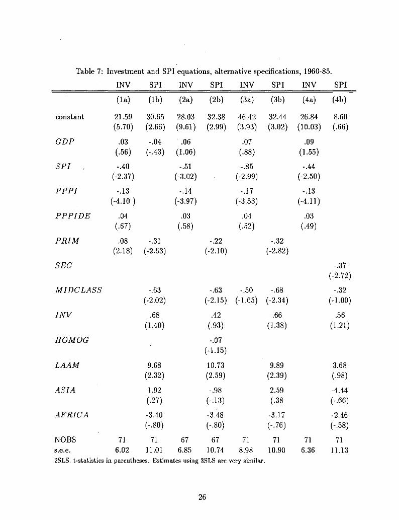
Table 7: Investment and SPI equations, alternative specifications, 1960-85.

INV SPI INV SPI INV SPI INV SPI

constant

GDP

SPI .

PPPI

PPPIDE

PRIM

SEC

MIDCLASS

INV

HOMOG

LAAM

ASIA

AFRICA

NOBSs.e.e.

(la)

21.59(5.70)

.03(.56)

-.40(-2.37)

-.13(-4.10 )

.04(.67)

.08(2.18)

716.02

(lb)

30.65(2.66)

-.04(-.43)

-.31(-2.63)

-.63(-2.02)

.68(1.40)

9.68(2.32)

1.92(.27)

-3.40(-.80)

7111.01

(2a)

28.03(9.61)

.06(1.06)

-.51(-3.02)

-.14(-3.97)

.03(.58)

676.85

(2b)

32.38(2.99)

-.22(-2.10)

-.63(-2.15)

.42(.93)

-.07(-1.15)

10.73(2.59)

-.98(-.13)

-3.48(-.80)

6710.74

(3a)

46.42(3.93)

.07(.88)

-.85(-2.99)

-.17(-3.53)

.04(.52)

-.50(-1.65)

718.98

(3b)

32.44(3.02)

-.32(-2.82)

-.68(-2.34)

.66(1.38)

9.89(2.39)

2.59(.38

-3.17(-.76)

7110.90

(4a)

26.84(10.03)

.09(1.55)

-.44(-2.50)

-.13(-4.11)

.03(.49)

716.36

(4b)

8.60(.66)

-.37(-2.72)

-.32(-1.00)

.56(1.21)

3.68(.98)

-4.44(-.66)

-2.46(-.58)

7111.13s.e.e. 6.02 11.01 6.85 10.74 8.98

2SLS. t-statistics in parentheses. Estimates using 3SLS are very similar.

26

Table 8: Investment and SPI equations, robust estimation, 1960-85.

INV SPI INV SPIG

constant

GDP

SPI

SPIG

PPPI

PPPIDE

PRIM

MIDCLASS

INV

LAAM

ASIA

AFRICA

NOBSs.e.e.rel. efF.

( la ) '

27.29(8.66)

.06(.83)

-.59(-3.15)

-.14(-3.62)

.05(.70)

717.21.94

(lb)

24.99(2.79)

-.22(-2.38)

-.49(-2.02)

.30(.73)

7.59(2.21)

3.17(.96)

-.86(-.25)

7110.34.87

(2a)

54.35(5.57)

-.02(-.28)

-1.12(-3.35)

-.12(-3.51)

.01(.13)

696.39.94

(2b)

36.78(8.04)

-.13(-2.71)

-.34(-2.78)

.14(.68)

1.49(.86)

3.62(1.05)

-1.11(-.63)

694.03.87

2SLS, using the Krasker-Welsh robust estimator, t-statistics in

parentheses.

27

References

AGHION, PHILLIP and PATRICK BOLTON [1991]: A Trickle-Down Theory of Growth

and Development with Debt-Overhang, mimeo;

ALESINA, ALBERTO and DANI RODRIK [1993]: Income Distribution and Economic

Growth: A Simple Theory and Some Empirical Evidence, in: Cukierman, Alex, Zvi Her-

covitz and Leonardo Leiderman: The Political Economy of Business Cycles and Growth,

MIT Press, Cambridge;

ALESINA, ALBERTO and DANI RODRIK [1994]: Distributive Politics and Economic

Growth, Quarterly Journal of Economics, forthcoming;

ALESINA, ALBERTO, SULE OZLER, NOURIEL ROUBINI and PHILIP SWAGEL

[1992]: Political Instability and Economic Growth, NBER working paper;

ALESINA, ALBERTO and GUIDO TABELLINI [1989]: External Debt, Capital Flights

and Political Risk, Journal of Inernational Economics, 27, 199-220;

BANERIJEE, ABHIJIT and ANDREW NEWMAN [1991]: Risk Bearing and the The-

ory of Income Distribution, Review of Economic Stuides, 58 211-35;

BARRO, ROBERT J. [1990]: Government Spending in a Simple Model of Endogenous

Growth, Journal of Political Economy 98 S103- 25;

BARRO, ROBERT J. [1991]: Economic Growth in a Cross-Section of Countries, Quar-

terly Journal of Economics 106 407-44;

BARRO, ROBERT J. and JONG-WAA LEE [1993]: International Comparisons of

Educational Attainments, Harvard University, unpublished;

BENHABIB, JESS and ALDO RUSTICHINI [1991]: Social Conflict, Growth and In-

come Distribution, mimeo;

BENHABIB, JESS and MARK SPIEGEL [1992]: The Role of Human Capital and

Political Instability in Economic Development, Economic Research Report, C.V. Starr

Center for Applied Economics, New York University;

BERG, ANDY and JEFFREY SACHS [1988]: The Debt Crisis: Structural Explana-

tions of Country Performance, Journal of Development Economics, 29, 271-306;

BERTOLA, GIUSEPPE [1994]: Market Structure and Income Distribution in Endoge-

nous Growth Models, American Economic Review;

CANNING, DAVID and MARIANNE FAY [1993]: Growth and Infrastructure, Columbia

University, unpublished;

CUKIERMAN, ALEX, SEBASTIAN EDWARDS and GUIDO TABELLINI [1992]:

Seigniorage and Political Stability, American Economic Review 82 537-555;

28

DEVARAJAN, SHANTAYAMAN, SWAROOP VINAYA and HENG-FU ZOU [1992]:

What Do Governments Buy?, unpublished manuscript, The World Bank;

EDWARDS, SEBASTIAN and GUIDO TABELLINI [1991]: Political Instability, Polit-

ical Weakness and Inflation: An Empirical Analysis, NBER wp 3721;

FAY, MARIANNE [1993]: Illegal Activities and Income Distribution: A Model with

Envy, mimeo, Columbia University;

FERNANDEZ, RAQUELand RICHARD ROGERSON [1991]: On the Political Econ-

omy of Educational Subsididies, mimeo, Hoover Institutions;

GALOR, ODED and JOSEPH ZEIRA [1988]: Income Distribution and Macroeco-

nomics, Brown University Working paper 89-25;

GUPTA, DIPAK K. [1990]: The Economics of Political Violence, Praeger, New York;

HIBBS, DOUGLAS [1973]: Mass Political Violence: a Cross-Sectional Analysis, Wiley

and Sons, New York;

HUNTINGTON, SAMUEL [1968]: Political Order in Changing Societies, Yale Univer-

sity Press, New Haven;

JAIN, SHAIL [1975]: Size Distribution of Income: A Compilation of Data, World Bank,

Washington, D.C.;

JODICE, D. and D.L. TAYLOR [1988]: World Handbook of Social and Political Indi-

cators, Yale University Press, New Haven;

KALDOR, NICHOLAS [1956]: Alternative Theories of Distribution, Review of Eco-

nomic Studies 23, 83-100;

KUH, EDWIN and ROY E. WELSCH [1980]: Econometric Models and Their As-

sessment for Policy: Some New Diagnostics Applied to the Translog Energy Demand in

Manufacturing, in S. Gass, ed.,: Proceedings of the Workshop on Validation and Assess-

ment Issues of Energy Models, National Bureau of Economic Standards, Washington, D.C.,

445-475;

KRASKER, WILLIAM S. and ROY E. WELSCH [1982]: Efficient Bounded-Influence

Regression Estimation, Journal of the American Statistical Association, 77 595-604;

KRASKER, WILLIAM S., EDWIN KUH and ROY E. WELSCH [1983]: Estimation

with Dirty Data and Flawed Models, Ch. 11 in Griliches, Zvi and Michael Intrilligator,

eds.: Handbook of Econometrics, North Holland, Amsterdam;

LEVINE, ROSS and DAVID RENELT [1992]: A Sensitivity Analysis of Cross-Country

Growth Regressions, American Economic Review, 82, 942-63;

29

LONDEGRAN, JOHN and KEITH POOLE [1990]: Poverty, the Coup Trap and the

Seizure of Executive Power, World Politics, 92, 1-24;

LONDEGRAN, JOHN and KEITH POOLE [1991]: Leadership Turnover and Uncon-

stitutional Rule, unpublished;

MAURO, PAOLO [1993]: Political Instability, Growth and Investment, unpublished,

Harvard University

MELTZER, ALLAN H. and SCOTT F. RICHARD [1981]: A Rational Theory of the

Size of Government, Journal of Political Economy, 89 914-27;

MELTZER, ALLAN H. and SCOTT F. RICHARD [1983]: Tests of a Rational Theory

of the Size of Government, Public Choice 41 403-18;

OZLER, SULE and GUIDO TABELLINI [1991]: External Debt and Political Instabil-

ity, mimeo;

PEROTTI, ROBERTO [1993]: Political Equilibrium, Income Distribution, and Growth,

Review of Economic Studies, September;

PEROTTI, ROBERTO [1994]: Income Distribution and Growth: an Empirical Inves-

tigation, mimeo, Columbia University;

PERSSON, TORSTEN and GUIDO TABELLINI [1990]: Is Inequality Harmful for

Growth? Theory and Evidence, mimeo, Berkeley;

PETERS, STEPHEN C , ALEXANDER M. SAMAROV and ROY E. WELSCH [1982]:

Computational Procedures for Bounded-Influence and Robust Regression, Technical Report

No. 30, MIT Center for Computational Research in Economics and Management Science;

ROBERTS, KEVIN W.S. [1977]: Voting Over Income Tax Schedules, Journal of Public

Economics, 8 329-40;

ROMER, TOM [1975]: Individual Welfare, Majority Voting, and the Properties of a

Linear Income Tax, Journal of Public Economics 14 163-85;

SALA y MARTIN, XAVIER [1992]: Transfers, unpublished manuscript;

THEIL, HENRI [1971]: Principles of Econometrics, John Wiley, New York;

VENIERIS, YANNIS and DIPAK GUPTA [1983]: Socio-Political and Economic Di-

mensions of Development: A Cross-Sectional Model, Economic Development and Cultural

Change, 31, 727-56;

VENIERIS, YANNIS and DIPAK GUPTA [1986]: Income Distribution and Socio-

Political Instability as Determinants of Savings: A Cross-Sectional Model, Journal of Po-

litical Economy, 96, 873-83;

VENIERIS, YANNIS and SAMUEL SPERLING [1989]: Saving and Socio-Political

30

Instability in Developed and Less-Developed Nations, unpublished manuscript;

31

1994-1995 Discussion Paper SeriesDepartment of Economics

Columbia University1022 International Affairs Bldg.

420 West 118th StreetNew York, N.Y., 10027

The following papers are published in the 1994-95 Columbia University Discussion Paper serieswhich runs from early November to October 31 (Academic Year). Domestic orders for discussionpapers are available for purchase at $8.00 (US) each and $140.00 (US) for the series. Foreign orderscost $10.00 (US) for individual paper and $185.00 for the series. To order discussion papers, pleasesend your check or money order payable to Department of Economics, Columbia University to theabove address. Be sure to include the series number for the paper when you place an order.

708. Trade and Wages: Choosing among Alternative ExplanationsJagdish Bhagwati

709. Dynamics of Canadian Welfare ParticipationGarrey F. Barret, Michael I. Cragg

710. Much Ado About Nothing? Capital Market Reaction to Changes inAntitrust Precedent concerning Exclusive Territories.Sherry A. Glied, Randall S. Kroszner

711. The Cost of DiabetesMatthew Kahn

712. Evidence on Unobserved Polluter Abatement EffortMatthew E. Kahn

713. The Premium for Skills: Evidence from MexicoMichael Cragg

714. Measuring the Incentive to be HomelessMichael Cragg, Mario Epelaum

715. The WTO: What Next?Jagdish Bhagwati

716. Do Converters Facilitate the Transition to a New Incompatible Technology?A Dynamic Analysis of ConvertersJay Phil Choi

716A. Shock Therapy and After: Prospects for Russian ReformPadma Desai

717. Wealth Effects, Distribution and The Theory of Organization-Andrew F. Newman and Patrick Legros

1994-95 Discussion Paper Series

718. Trade and the Environment: Does Environmental Diversity Detract from the Case forFree Trade?-Jagdish Bhagwati and T.N. Srinivasan (Yale Univ)

719. US Trade Policy: Successes and Failures-Jagdish Bhagwati

720. Distribution of the Disinflation of Prices in 1990-91 Compared with Previous BusinessCycles-Philip Cagan

721. Consequences of Discretion in the Formation of Commodities Policy-John McLaren

722. The Provision of (Two-Way) Converters in the Transition Process to a New IncompatibleTechnology-Jay Pil Choi

723. Globalization, Sovereignty and Democracy-Jagdish Bhagwati

724. Preemptive R&D, Rent Dissipation and the "Leverage Theory"-Jay Pil Choi

725. The WTO's Agenda: Environment and Labour Standards, Competition Policy and theQuestion of Regionalism-Jagdish Bhagwati

726. US Trade Policy: The Infatuation with FT As-Jagdish Bhagwati

727. Democracy and Development: New Thinking on an Old Question-Jagdish Bhagwati

728. The AIDS Epidemic and Economic Policy Analysis-David E. Bloom, Ajay S. Mahal

729. Economics of the Generation and Management of Municipal Solid Waste-David E. Bloom, David N. Beede

730. Does the AIDS Epidemic Really Threaten Economic Growth?-David E. Bloom, Ajay S. Mahal

731. Big-City Governments-Brendan O'Flaherty

732. International Public Opinion on the Environment-David Bloom

1994-95 Discussion Paper Series

733. Is an Integrated Regional Labor Market Emerging in the East and Southeast Asia?-David Bloom, Waseem Noor

734. Migration, Integration and Development-Abhijit V. Banerjee, Andrew Newman

735. Infrastructure, Human Capital and International Trade-Ronald Findlay

736. Short Ballots: Why Mayors Are in Charge of So Many Different Things-Brendan O'Flaherty

737. Demand for Environmental Goods: Evidence from Voting Patterns on California Initiatives-Matthew Kahn and John Matsusaka

738. Inflation and Stabilization in Poland 1990 - 1995-S.Wellisz

739. Paniculate Pollution Trends in the 1980's-M. Kahn

740. Why has Wage Dispersion Grown in Mexico? Is it the Incidence of Reforms or theGrowing Demand for Skills?-M.I. Cragg and M. Epelbaum

741. Russia's Transition Toward the World Economy:-P. Desai

742. Poland: Transition and Integration in the World Economy-S. Wellisz

743. Team Effects on Compensation: An Application to Salary Determination in the National HockeyLeague-T. Idson and L.H. Kahane

744. Economic Development, Growth of Human Capital, and the Dynamics of the Wage Structure-J. Mincer

745. Technology Transfer with Moral Hazard-J.P. Choi (Oct.)

746. Risk Preference Smoothness and the APT-L.F. Herk, Columbia University, Institute on East Central Europe

747. A Characterization of Cointegration-P. Dhrymes (Oct.)

748. The Limiting Distribution of the Cointegration-P. Dhrymes (Oct.)

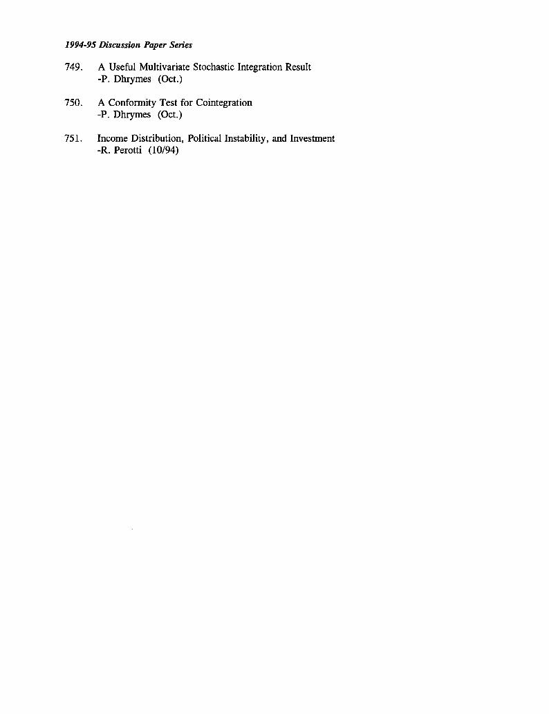
1994-95 Discussion Paper Series

749. A Useful Multivariate Stochastic Integration Result-P. Dhrymes (Oct.)

750. A Conformity Test for Cointegration-P. Dhrymes (Oct.)

751. Income Distribution, Political Instability, and Investment-R. Perotti (10/94)