income and substitution effects in consumer goods markest · pdf filegraph7.2: gasoline and...

C H A P T E R

7Income and Substitution Effects inConsumer Goods Markest

In Chapter 6 we showed how economic circumstances combine with tastes to re-

sult in choice or behavior. In Chapter 7 we show how consumer choices (and thus

the consumer behavior we observe) change as circumstances change — i.e. as in-

comes and prices change. Put differently, we will now show how “people respond

to incentives” in the consumer goods market.

Chapter HighlightsThe main points of the chapter are:

1. There are two ways in which economic circumstances typically change: a

change in income and a change in opportunity costs.

2. When only income changes, we can predict the change in behavior if we

know something about how indifference curves relate to one another — be-

cause we jump from one indifference curve to another. Whether tastes are

quasilinear or homothetic, whether goods are normal or inferior — these are

statements about that relationship between indifference curves.

3. When only opportunity costs change and real income remains constant, we

don’t need to know anything about the relationship of indifference curves to

one another — because the change in behavior occurs along a single indif-

ference curve. Thus, the shape of the relevant indifference curve is all that

matters — which is the same as saying that the degree of substitutability of

the goods at the margin is all that matters.

4. Substitution effects arise as we slide along indifference curves because op-

portunity costs have changed; income effects arise as we jump between in-

difference curves because real income has changed.

61 7A. Solutions to Within-Chapter-Exercises

5. Price changes give rise to both of these effects. To identify the substitution

effect, we only look at the initial indifference curve and thus need to know

about the substitutability of goods at the margin; to identify income effects,

we have to know how indifference curves relate to one another.

Using the LiveGraphsFor an overview of what is contained on the LiveGraphs site for each of the chapters

(from Chapter 2 through 29) and how you might utilize this resource, see pages 2-3

of Chapter 1 of this Study Guide. To access the LiveGraphs for Chapter 7, click the

Chapter 7 tab on the left side of the LiveGraphs web site.

In addition to the Animated Graphics, Static Graphics and Downloads portions

of the LiveGraphs site, this Chapter has several Exploring Relationships modules:

1. The module titled “The Income and Substitution Effect for Two Goods” al-

lows you to review all possible 2-good gases for income and substitution ef-

fects.

2. The two modules labeled Interactive Application allow you to practice with

income effects (in the application entitled “Normal/Inferior Goods – Income

Change”) and with both income and substitution effects (in the application

entitled “The Income and Substitution Effect Game”).

7A Solutions to Within-Chapter-Exercises

Exercise 7A.1 Is it also the case that whenever there is a positive income effect on our con-

sumption of one good, there must be a negative income effect on our consumption of a differ-

ent good?

Answer: No — since it is possible for our consumption of all goods to go up as

income increases, the income effect could be positive for all goods.

Exercise 7A.2 Can a good be an inferior good at all income levels? (Hint: Consider the bundle

(0,0).)

Answer: No. The reason is that, in order for a good to be inferior, it must be

that you consume more of it as income falls. But, as income falls toward zero, at

some point it will not be possible to consume more as income falls — because there

simply won’t be enough income to consume more. Thus, around the origin, no

good can be inferior.

Income and Substitution Effects in Consumer Goods Markest 62

Exercise 7A.3 Are all inferior goods necessities? Are all necessities inferior goods? (Hint: The

answer to the first is yes; the answer to the second is no.) Explain.

Answer: If you consume less of a good as income goes up, then it must be true

that you spend a smaller fraction of your income on that good as income goes up.

Thus, all inferior goods are necessities. At the same time, it may be the case that the

fraction of your income spent on a good declines as your income goes up — but

you still buy more of the good. (For instance, suppose your income goes up by 10%

and you choose to consume 5% more of a good. Then the fraction of income spent

on that good is declining even though you are increasing your consumption of the

good as your income goes up.) Thus, necessities could be normal goods.

Exercise 7A.4 At a particular consumption bundle, can both goods (in a 2-good model) be

luxuries? Can they both be necessities?

Answer: No. In a 2-good model, you will end up spending all your income as

income increases. So suppose you are currently spending all your income on the

two goods and your income now increases by 10%. If your consumption of both

goods increases by more than 10%, then you would now be spending more than

your new income. If your consumption of both goods increases by less than 10%,

you would be spending less than your new income.

Exercise 7A.5 If you knew only that my brother and I had the same income (but not necessarily

the same tastes), could you tell which one of us drove more miles — the one that rented or the

one that took taxis?

Answer: Yes. Suppose my brother faces the intersecting budget lines — with the

steeper one representing taxis and the shallower one representing rental cars. He

chooses the steeper (taxi) budget line. Then we know that he must be consuming a

bundle to the left of the intersection point of the two lines — because if he chose to

the right of that point, he could have had more of everything on the shallower bud-

get and thus should have chosen the shallower (rental car) budget instead. Thus,

by choosing the steeper taxi budget, we know my brother consumes to the left of

the intersection point. I, on the other hand, chose the shallower rental car budget.

If I were to then choose a bundle to the left of the intersection point, I could have

done better choosing the steeper budget because I could get more of both goods.

Thus I must be consuming to the right of the intersection point. If my brother and

I have the same incomes (and thus face the same taxi and rental car budgets), it

therefore must be the case that my brother consumes to the left of the intersection

point on the taxi budget and I consume to the right on the rental car budget. We

can unambiguously say I consumed more miles driven.

Exercise 7A.6 True or False: If you observed my brother and me consuming the same number

of miles driven during our vacations, then our tastes must be those of perfect complements

between miles driven and other consumption.


Answer: It would at a minimum have to be the case that the indifference curve

at the intersection of the two budget lines has a sharp kink at that point. That kink

could be such that it forms a right angle — thus creating the typical perfect com-

plements indifference curve. But at a minimum it has to be such that the upper

part of the indifference curve is steeper than the taxi budget and the lower part is

shallower than the rental car budget — with a kink at the intersection.

Exercise 7A.7 Can you re-tell the Heating Gasoline-in-Midwest story in terms of income and

substitution effects in a graph with “yearly gallons of gasoline consumption” on the horizontal

axis and “yearly time on vacation in Florida” on the vertical?

Answer: In panel (a) of Graph 7.1, bundle A is the original consumption bundle

prior to the increase in the price of gasoline. The increase in the price of gasoline

then rotates the budget clockwise. Bundle B lies on the compensated budget at

the new price of gasoline — and the move from A to B is the substitution effect.

As always, the substitution effect causes a decrease in consumption of the good

(gasoline) that has become more expensive.

Graph 7.1: Gasoline and Florida Vacation Time

Panel (b) illustrates C — with no consumption of Florida vacation time. This

corner solution is rationalized by an indifference curve that crosses the new budget

at C — creating an income effect in the opposite direction of the substitution effect.

Since the income effect is larger than the substitution effect, the consumer shifts

from A before the increase in the price of gasoline to C after the price increase —

with an overall increase in gasoline consumption resulting from the price increase.

Exercise 7A.8 Replicate Graph 7.7 for an increase in the price of pants (rather than a decrease).


Answer: Panel (a) of Graph 7.2 illustrates the original consumption bundle A

and the change in the budget constraint when the price of pants increases. Panel

(b) illustrates the compensated budget and the resulting bundle B — with the sub-

stitution effect as the movement from A to B . As always, this effect says the con-

sumer will consume less of what has become more expensive, more of what has

become relatively cheaper. Finally, panel (c) identifies four regions (labeled 1, 2,

3 and 4) on the new (uncompensated) budget line. If the consumer ends up opti-

mizing in region 1, her consumption of pants decreases and her consumption of

shirts increases with a decline in income (relative to the compensated budget) —

which implies that pants are a normal good and shirts are inferior. In region 2, the

consumption of both goods declines with income — thus both pants and shirts are

normal goods. In regions 3 and 4, consumption of shirts decreases and consump-

tion of pants increases with a drop in income (from the compensated budget) —

thus making shirts normal and pants inferior. In region 3, however, the consumer

still buys fewer pants as the price increases (i.e. C is to the left of A) — which means

pants are regular inferior; in region 4, on the other hand, pants consumption goes

up with an increase in price, which makes pants a Giffen good.

Graph 7.2: Gasoline and Florida Vacation Time

End of Chapter Exercises

Exercise 7.520 Return to the analysis of my undying love for my wife expressed through weekly purchases of roses (as

introduced in end-of-chapter exercise 6.4).

Recall that initially roses cost $5 each and, with an income of $125 per week, I bought 25 roses each

week. Then, when my income increased to $500 per week, I continued to buy 25 roses per week (at

the same price).


(a) From what you observed thus far, are roses a normal or an inferior good for me? Are they a

luxury or a necessity?

Answer: As income went up, my consumption remained unchanged. This would typically

indicate that the good in question is borderline normal/inferior — or quasilinear. Since the

consumption at the lower income is at a corner solution, however, we cannot be certain

that the good is not inferior, with the MRS at the original optimum larger in absolute value

than the MRS at the new (higher income) optimum. Regardless, roses must be a necessity

— whether they are borderline inferior/normal or inferior, the percentage of income spent

on roses declines as income increases.

(b) On a graph with weekly roses consumption on the horizontal and “other goods” on the ver-

tical, illustrate my budget constraint when my weekly income is $125. Then illustrate the

change in the budget constraint when income remains $125 per week and the price of roses

falls to $2.50. Suppose that my optimal consumption of roses after this price change rises to

50 roses per week and illustrate this as bundle C.

Answer: This is illustrated in panel (a) of Graph 7.3 where A is the original corner solution,

C is the new corner solution and the dashed line is the compensated budget.

Graph 7.3: Love and Roses

(c) Illustrate the compensated budget line and use it to illustrate the income and substitution

effects.

Answer: This is also illustrated in panel (a) of the graph. In this case, there is no substitution

effect (in terms of roses) and only an income effect.

(d) Now consider the case where my income is $500 and, when the price changes from $5 to $2.50,

I end up consuming 100 roses per week (rather than 25). Assuming quasilinearity in roses,

illustrate income and substitution effects.

Answer: This is illustrated in panel (b) of Graph 7.3 where the dashed line is again the com-

pensated budget line. Unlike in panel (a), the entire change in roses consumption is now

due to a substitution effect rather than an income effect.

(e) True or False: Price changes of goods that are quasilinear give rise to no income effects for the

quasilinear good unless corner solutions are involved.

Answer: This is true. We will often make the statement that income effects disappear if

we assume quasilinearity of a good — because then a good is borderline normal/inferior,

which implies consumption remains unchanged as income changes. This is true so long as

the consumer is at an interior solution. If quasilinear tastes lead to corner solutions, then

this may give rise to income effects as we see in panel (a) of the graph.


Exercise 7.8: Sam’s Club and the Marginal Consumer21 Business Application: Sam’s Club and the Marginal Consumer: Superstores like Costco and Sam’s Club

serve as wholesalers to businesses but also target consumers who are willing to pay a fixed fee in order to

get access to the lower wholesale prices offered in these stores. For purposes of this exercise, suppose that

you can denote goods sold at Superstores as x1 and “dollars of other consumption” as x2.

Suppose all consumers have the same homothetic tastes over x1 and x2 but they differ in their in-

come. Every consumer is offered the same option of either shopping at stores with somewhat higher

prices for x1 or paying the fixed fee c to shop at a Superstore at somewhat lower prices for x1.

(a) On a graph with x1 on the horizontal axis and x2 on the vertical, illustrate the regular budget

(without a Superstore membership) and the Superstore budget for a consumer whose income

is such that these two budgets cross on the 45 degree line. Indicate on your graph a vertical

distance that is equal to the Superstore membership fee c.

Answer: In panel (a) of Graph 7.4, the Superstore budget has shallower slope (because of the

lower price of x1) but a lower vertical intercept (because of the fixed membership fee). The

lower two budgets in the graph are such that they intersect on the 45 degree line.

Graph 7.4: Sam’s Club

(b) Now consider a consumer with twice that much income. Where will this consumer’s two bud-

gets intersect relative to the 45 degree line?

Answer: This is also illustrated in panel (a). When income is doubled, the vertical intercept

of the regular budget doubles — but the vertical intercept of the Superstore budget more

than doubles because the fixed fee remains the same. (If the initial income is I , the initial

intercept of the Superstore budget is (I − c). When income doubles, the new intercept is

(2I − c) — which is greater than 2(I − c).) For this reason, the two budget lines will cross

above the 45 degree line when income doubles.

(c) Suppose consumer 1 (from part (a)) is just indifferent between buying and not buying the

Superstore membership. How will her behavior differ depending on whether or not she buys

the membership.

Answer: In panel (b) of the graph, Consumer 1 will then consume at bundle A if she does

not buy the membership and at bundle B if she does. This is a pure substitution effect —

with greater consumption when price is lower.

(d) If consumer 1 was indifferent between buying and not buying the Superstore membership,

can you tell whether consumer 2 (from part (b)) is also indifferent? (Hint: Given that tastes

are homothetic and identical across consumers, what would have to be true about the inter-

section of the two budgets for the higher income consumer in order for the consumer to also

be indifferent between them?)


Answer: Consumer 2 will then definitely buy the membership. This is also illustrated in

panel (b) of Graph 7.4 where C is the optimal bundle on the regular budget and D is the

optimal bundle on the Superstore budget for the higher income consumer. (These optimal

bundles lie along rays from the origin going through A and B because we are assuming

that tastes are homothetic). Because of the different relationship between the two budgets

for the lower and higher income consumers (as identified in panel (a)), D lies on a higher

indifference curve than C — implying that consumer 2 will buy the membership.

(e) True or False: Assuming consumers have the same homothetic tastes,there exists a “marginal”

consumer with income I such that all consumers with income greater than I will buy the

Superstore membership and no consumer with income below I will buy that membership.

Answer: This is true. Higher income consumers whose two budgets will intersect above the

45 degree line will be better off on the Superstore budget (as illustrated in panel (b)). For

analogous reasons, lower income consumers will face that intersection point below the 45

degree line — causing the regular budget to yield an optimum with greater utility than the

Superstore budget.

(f) True or False: By raising c and/or p1, the Superstore will lose relatively lower income cus-

tomers and keep high income customers.

Answer: True. Suppose we begin again with Consumer 1 who is indifferent and whose bud-

get lines are illustrated again in panel (c) of Graph 7.4. An increase in c will cause the shal-

lower Superstore budget to shift in parallel — causing the two budgets to intersect below

the 45 degree line and leaving Consumer 1 better off on the regular budget (where she can

still consume at A). If p1 increases in the Superstore, the slope of the Superstore budget

becomes steeper — again causing the intersection point to fall below the 45 degree line and

leaving Consumer 1 better off at A under the regular budget. Thus, the marginal consumer

will cease shopping at the Superstore if c or p1 are increased. Because of the homothetic-

ity assumption, we also know that the new marginal consumer will again have her budgets

intersect on the 45 degree line — and we have seen in panel (a) that this intersection point

moves up on the regular budget as income increases. If an increase in c or p1 have caused

the intersection point to slide below the 45 degree line for the original marginal consumer,

then an increase in income will cause it to slide back up. Thus, there exists some higher

income level at which we will find our new marginal consumer.

(g) Suppose you are a Superstore manager and you think your store is overcrowded. You’d like to

reduce the number of customers while at the same time increasing the amount each customer

purchases. How would you do this?

Answer: You would want to increase c — which will raise the income of your marginal con-

sumer and reduce the overall number of consumers with memberships. Then, in order to

get your members to shop more, you would lower p1 — but not so much that membership

again goes up by too much. You can see that this is possible by again looking at panel (c)

of the graph. By increasing c , you insure that this marginal consumer will no longer be a

member. You can then lower price (which will make the new budget shallower) and keep

the marginal consumer from coming back to your store so long as you don’t lower the prices

too much.

Exercise 7.12: Fuel Efficiency, Gasoline Consumption,and Gas Prices

22 Policy Application: Fuel Efficiency, Gasoline Consumption and Gas Prices: Policy makers frequently

search for ways to reduce consumption of gasoline. One straightforward option is to tax gasoline —

thereby encouraging consumers to drive less in their cars and switch to more fuel efficient cars.

Suppose that you have tastes for driving and for other consumption, and assume throughout that

your tastes are homothetic.

(a) On a graph with monthly miles driven on the horizontal and “monthly other consumption”

on the vertical axis, illustrate two budget lines: One in which you own a gas-guzzling car

— which has a low monthly payment (that has to be made regardless of how much the car


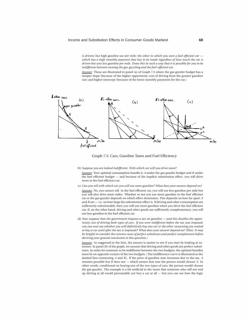
is driven) but high gasoline use per mile; the other in which you own a fuel efficient car —

which has a high monthly payment that has to be made regardless of how much the car is

driven but uses less gasoline per mile. Draw this in such a way that it is possible for you to be

indifferent between owning the gas-guzzling and the fuel-efficient car.

Answer: These are illustrated in panel (a) of Graph 7.5 where the gas guzzler budget has a

steeper slope (because of the higher opportunity cost of driving from the greater gasoline

use) and higher intercept (because of the lower monthly payments for the car.)

Graph 7.5: Cars, Gasoline Taxes and Fuel Efficiency

(b) Suppose you are indeed indifferent. With which car will you drive more?

Answer: Your optimal consumption bundle is A under the gas guzzler budget and B under

the fuel efficient budget — and because of the implicit substitution effect, you will drive

more in the fuel efficient car.

(c) Can you tell with which car you will use more gasoline? What does your answer depend on?

Answer: No, you cannot tell. In the fuel efficient car, you will use less gasoline per mile but

you will also drive more miles. Whether or not you use more gasoline in the fuel efficient

car or the gas guzzler depends on which effect dominates. This depends on how far apart A

and B are — i.e. on how large the substitution effect is. If driving and other consumption are

sufficiently substitutable, then you will use more gasoline when you drive the fuel efficient

car; if, on the other hand, driving and other goods are sufficiently complementary, you will

use less gasoline in the fuel efficient car.

(d) Now suppose that the government imposes a tax on gasoline — and this doubles the oppor-

tunity cost of driving both types of cars. If you were indifferent before the tax was imposed,

can you now say whether you will definitively buy one car or the other (assuming you waited

to buy a car until after the tax is imposed)? What does your answer depend on? (Hint: It may

be helpful to consider the extreme cases of perfect substitutes and perfect complements before

deriving your general conclusion to this question.)

Answer: As suggested in the hint, the answer is easiest to see if you start by looking at ex-

tremes. In panel (b) of the graph, we assume that driving and other goods are perfect substi-

tutes. In order for someone to be indifferent between the two budgets, the optimal bundles

must lie on opposite corners of the two budgets. (The indifference curve is illustrated as the

dashed line connecting A and B ). If the price of gasoline now increases due to the tax, A

remains possible but B does not — which means that now the person would choose A. In

other words, conditional on buying one of the two types of cars, the person would choose

the gas guzzler. The example is a bit artificial in the sense that someone who will not end

up driving at all would presumably not buy a car at all — but you can see how the logic


also holds for tastes that are close to perfect substitutes where the consumer would choose

interior solutions.

In panel (c) of the graph, we go to the other extreme — with tastes over miles and other

consumption modeled as perfect complements. In that case, A=B to begin with — and

when gasoline prices go up, the fuel efficient car becomes unambiguously better (with the

optimum at C and all bundles on the after-tax gas guzzling budget falling below uC .)

Upon reflection, this should make intuitive sense. If miles and other consumption are rel-

atively complementary, then it makes sense to switch to a more fuel efficient car because

we want to keep driving quite a bit even if the price of gasoline increases. If, on the other

hand, miles and other consumption are relatively substitutable, then one way to respond to

a price increase is to substitute away from gasoline altogether and just drive very little. With

only a little driving each month, it’s better to pay the lower fixed cost of the gas guzzler even

if each mile costs more.

(e) The empirical evidence suggests that consumers shift toward more fuel efficient cars when the

price of gasoline increases. True or False: This would tend to suggest that driving and other

good consumption are relatively complementary.

Answer: True — based on the explanation to part (d) above.

(f) Suppose an increase in gasoline taxes raises the opportunity cost of driving a mile with a fuel

efficient car to the opportunity cost of driving a gas guzzler before the tax increase. Would

someone with homothetic tastes drive more or less in the fuel efficient car after the tax increase

than she would in a gas guzzler prior to the tax increase?

Answer: The person would drive less in the fuel efficient car after the tax increase than in

the gas guzzler before the tax increase. You can illustrate this simply by drawing the gas

guzzler budget before the tax and the fuel efficient budget after the tax. You should get both

budgets to have the same slope (because of the same opportunity cost of driving) — but the

fuel efficient car has lower intercept because of the higher monthly payments. This is then

a pure income effect — with the new optimal bundle on the after-tax fuel efficient budget

lying on the same ray from the origin as the original optimal bundle before-tax gas guzzler

budget. The new bundle then necessarily lies to the left of the original.

Conclusion: Potentially Helpful Reminders1. Important Graphing Hint: When graphing income and substitution effects,

it is very helpful to draw the original indifference curve with lots of substi-

tutability — i.e. with relatively little curvature — unless specifically told to

do otherwise. If you do this, it becomes much harder to trick yourself into

thinking that something which is logically impossible is actually happening

in your graphs.

2. Keep in mind the following: Substitution effects always occur along a single

indifference curve and income effects always involve jumping from one indif-

ference curve to another across two parallel budgets.

3. Since concepts like homotheticity, quasilinearity, normal and inferior goods,

and luxuries and necessities are definitions about how indifference curves

within an indifference map relate to one another, they are relevant only for

determining income effects. In fact, we can get both large and small substi-

tution effects for any of these types of tastes and goods — with the size of

the substitution effect depending on the curvature of the original indiffer-


ence curve (which has no relation to whether goods are normal or inferior or

homothetic, etc.).

4. In the text, we emphasize the more common of the two types of substitu-

tion effects that economists talk about — the effect that holds “real welfare”

fixed and thus occurs along an indifference curve. This effect is also called the

Hicks substitution effect and it differs from a second type of substitution effect

(called the Slutsky substitution effect) that assumes a consumer is compen-

sated enough to afford the original bundle (rather than to reach the original

indifference curve). This second type of substitution effect is almost identi-

cal to the first, particularly for small changes in prices — and it appears in

end-of-chapter exercises 7.6 and 7.11 for you to explore.

5. Often students confuse Giffen goods with a certain type of “prestige good”

that people value more as it gets more expensive. That is definitely not what a

Giffen good is — and you can do end-of-chapter exercise 7.9 to work through

the difference between these two types of goods.

income and substitution effects in consumer goods markest · pdf filegraph7.2: gasoline and...

Documents