in - naval postgraduate school vitae searchfaculty.nps.edu/dad/orbital/satellite.pdfen in terms of...
TRANSCRIPT

SATELLITE MOTION AROUND AN OBLATE
PLANET� A PERTURBATION SOLUTION FOR
ALL ORBITAL PARAMETERS
D� A� Danielson� ProfessorG� E� Latta� Professor
C� P� Sagovac� LT� U�S� NavyS� D� Krambeck� LT� U�S� NavyJ� R� Snider� LTC� U�S� ArmyMathematics DepartmentNaval Postgraduate SchoolMonterey� California �����
Abstract
The search for a universal solution of the equations of motion for a
satellite orbiting an oblate planet is a subject that has merited great
interest because of its theoretical and practical implications� Here� a
complete �rst�order perturbation solution� including the e�ects of the
J� terms in the planet�s potential� is given in terms of standard orbital
parameters� The simple formulas provide a fast method for predict�
ing satellite orbits that is more accurate than the two�body formulas�
These predictions are shown to agree well with those of a completely
numerical code and with actual satellite data� Also� in an appendix� it
is rigorously proven that a satellite having negative mechanical energy
remains for all time within a spherical annulus with radii approximately
equal to the perigee and apogee of its initial osculating ellipse�

� Introduction
A characteristic feature of practical orbit prediction is that the engineer may deal with
numerous satellites in a great variety of orbits� Under these circumstances analytical relations
which can quickly approximate an orbit may be far superior to large numerical programs�
While many analytical models have been developed for the arti�cial satellite age� most are
not used in practical orbit prediction because they violate one or more of the following
principles
� The method should provide a solution that is signi�cantly more accurate than thetwo�body solution�
� The real physical e�ects of the orbit should be easily distinguishable in the solution�
� The solution should be universal� it should be valid for all orbital parameters�
The problem of predicting the motion of a satellite perturbed only by the oblateness of the
planet has received considerable attention following the �rst launchings of arti�cial satellites
about the Earth� Some of the studies of this problem by means of general perturbation
theories are listed at the end of this paper� Techniques have involved expansions in powers
ofpJ�� averaging processes� the use of spheroidal coordinates� and the edi�ce of Hamiltonian
mechanics� It is not the intention of this present paper to compare the various methodologies
used� Su�ce it to say that many researchers believe a solution which embodies all of the
above principles was not achieved e�g�� see Ta���
The basic procedure used in this paper to solve the di�erential equations of motion is
the perturbation technique known as the Method of Strained Coordinates� This technique
was �rst applied to the title problem by Brenner� Latta� and Weis�eld� Using a mean orbital
plane to specify an arbitrary orbit� they were only able to obtain a partial solution e�g�� the
eccentricity was assumed small and initial conditions were not considered��
�

Here we use coordinates in the true orbital plane to cast the di�erential equations into a
simpli�ed form� as was originally done by Struble�
� Orbital Kinematics
Figure shows the usual reference system of spherical coordinates r� �� ��� The radial
distance r is measured from the center of the planet O to the satellite S� The line O� is in
a direction �xed with respect to an inertial coordinate system� The right ascension � is the
angle measured in the planet�s equatorial plane eastward from the line O�� The declination
or latitude � is the angle measured northward from the equator� The position vector r of
the satellite in the spherical coordinate system is
r � r cos� cos ��b� � r sin� cos ��b� � r sin��b� �
where b��b��b�� are orthonormal base vectors �xed in the directions shown�
We can also locate the satellite by its polar coordinates r� �� within a possibly rotating�
orbital plane that instantaneously contains its position and velocity vectors� Here � is the
argument of latitude� i�e�� the angle measured in the orbital plane from the ascending node to
the satellite� The orbital plane is inclined at an angle i to the equatorial plane and intersects
the equatorial plane in the line of nodes� making an angle � with the O� line�
We introduce another orthonormal set of base vectors B��B��B�� which move with the
satellite so that B� is in the direction of the position vector r� B� is also in the orbital plane�
and B� � B��B�� The basis b��b��b�� may be transformed into the basis B��B��B�� by
a succession of three rotations� First the basis b��b��b�� is rotated about the b� direction
by the angle �� next the basis is rotated about the new �direction by the angle i� and
�nally the basis is again rotated about the new ��direction by the angle �� The two sets of
base vectors are related by the product of the rotation matrices representing each successive
�
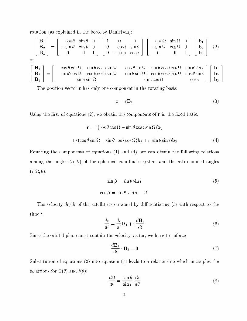
rotation as explained in the book by Danielson����B�
B�
B�
��� �
���cos � sin � �
� sin � cos � �� �
������ � �� cos i sin i� � sin i cos i
������cos � sin� �
� sin� cos� �� �
������b�
b�
b�
��� ��
or��� B�
B�
B�
��� �
��� cos � cos �� sin � cos i sin� cos � sin� � sin � cos i cos � sin � sin i� sin � cos �� cos � cos i sin� � sin � sin� � cos � cos i cos � cos � sin i
sin i sin� � sin i cos � cos i
������ b�
b�
b�
���
The position vector r has only one component in the rotating basis
r � rB� ��
Using the �rst of equations ��� we obtain the components of r in the �xed basis
r � r cos � cos �� sin � cos i sin��b�
�r cos � sin� � sin � cos i cos ��b� � r sin � sin i�b� ��
Equating the components of equations � and ��� we can obtain the following relations
among the angles �� �� of the spherical coordinate system and the astronomical angles
i��� ��
sin� � sin � sin i ��
cos � � cos � sec �� ��
The velocity dr�dt of the satellite is obtained by di�erentiating �� with respect to the
time t
dr
dt�
dr
dtB� � r
dB�
dt ��
Since the orbital plane must contain the velocity vector� we have to enforce
dB�
dt�B� � � ��
Substitution of equations �� into equation �� leads to a relationship which uncouples the
equations for � �� and i ��
d�
d��tan �
sin i
di
d� ��
�

The velocity �� can then be written
dr
dt�
dr
dtB� � r
d�
dt
� � tan � cot i
di
d�
�B� ��
In the following part of this paper� we will obtain expressions for r ��� i ��� � ��� and
dt�d� ��� The position and velocity vectors of the satellite then may be calculated from
the formulas in this section� The classical orbital elements p� e� and � are the semilatus
rectum� eccentricity� and argument of perigee of the instantaneous osculating� conic section
determined by the position and velocity vectors� If needed� p ��� e ��� and � �� can be
obtained from our solution r �� and dt�d� ��
p �r�
GM�dtd�
�
e cos � � �� �p
r�
e sin � � �� �p
r�
�dr
d�
�
� Equations of Motion
The expressions for the kinetic and potential energies per unit mass of a satellite orbiting
around an oblate planet are respectively
T �
�
���dr
dt
��
� r��d�
dt
��
� r� cos� �
�d�
dt
���� ��
V � �GM
r
�
J�R�
�r�
�� � sin� �
� �
where G is the gravitational constant� M is the mass of the planet� R is the equatorial radius
of the planet� and J� is the constant coe�cient of the spherical harmonic of degree � and
order � in the planet�s gravitational �eld� Substitution of these equations into Lagrange�s
equations
d
dt
� T � V �
��dq
dt
� �
�q T � V � � � q � r� �� or �
�

results in the following equations of motion
d�r
dt�� r
�d�
dt
��
� r cos� �
�d�
dt
��
� ��V
�r ��
d
dt
�r� cos� �
d�
dt
�� �
d
dt
�r�d�
dt
�� r� sin� cos �
�d�
dt
��
� ��V
�� ��
Initial conditions are established by requiring that at the initial time t� the orbital pa�
rameters of the usual two�body orbit� the conic section determined by the initial position and
velocity vectors� are known� The actual orbit is then tangent to this initial instantaneous
conic section at t� see Figure �� Equating the initial position and velocity vectors given by
equations �� and �� to the two�body expressions� we obtain
r t�� �p�
� e� cos �� � ���� ��
dr
dt t�� �
e�h� sin �� � ���
p� ��
d�
dt t�� �
h�
r��h � tan �� cot i�
did� ���
i ��
i ��� � i� ��
� ��� � �� ��
Here h� �pGMp� is the initial value of the satellite�s speci�c angular momentum about the
center of the planet� and the subscript � on a symbol denotes that the parameter is evaluated
at the initial time t��
We immediately have two integrals of the equations of motion
T � V � constant ��
r� cos� �d�
dt� constant ���
�

Equation �� simply states that the mechanical energy of the satellite remains constant�
Now� from equations � and ��
r� cos� �d�
dt� r� dr
dt� b� � h� cos i� ��
Equation �� simply states that the component along the polar axis of the speci�c angular
momentum of the satellite remains constant� Inserting equations �� and �� into equation
��� we obtain
dt
d��
r� cos i
h� cos i�
� � tan � cot i
di
d�
� ���
This allows the independent variable to be changed from t to ��
Letting u � p��r� and using equations ��� ��� and ���� we can rewrite the remaining
equations of motion ��� ��
di
d����Ju sin � cos � sin i cos� i
c�
cos i� �Ju sin� � cos� i
���
d�u
d��� u �
cos� i
c��
J cos� i
c�
�u� � � sin� � sin� i� � �udu
d�sin � cos � � � cos� i�
��ud�u
d��sin� � cos� i� �
�du
d�
��
sin� � cos� i � �J
�u sin� � cos� i
c� ���
udu
d�cos � � � sin� i� �
d
d�
�udu
d�
�sin � cos� i
�
The terms in ��� with d�u�d�� can be combined� yielding the equivalent equation
d�u
d��� u �
�cos� i
c��J cos� i
c��u� � sin� � � cos� i� ���
��udu
d�sin � cos � � � cos� i�� �
�du
d�
��
sin� � cos� i�
��J�u sin� � cos� i
c�
��u� sin � cos� i� u
du
d�cos � � � sin� i��
�du
d�
��
sin � cos� i
����� ���
�� ��Ju sin� � cos� i
c���J�u� sin� � cos� i
c�
�
�

Here we have introduced the shorthand notation c � cos i�� s � sin i�� J � �J�R���p�
��
� Perturbation Procedure
The di�erential equations ���� ��� are coupled by the nonlinear terms and apparently
cannot be solved analytically� If we expand the right sides of ��� and ��� in a Taylor series
expansion in powers of J and retain only terms up to order J�� the equations simplify to
di
d����Ju sin � cos � sin i cos� i
c���J�u� sin i cos� i
c�sin� � cos � �O J�� ���
d�u
d��� u �
cos� i
c��
J cos� i
c�
���u sin� � cos� ic�
� u�� � sin� � � cos� i� ���
��udu
d�sin � cos � � � cos� i�� �
�du
d�
��
sin� � cos� i�
���
��J�u sin� � cos� i
c�
�u��� � � sin� � � � cos� i�� � �u sin
� � cos� i
c�
�udu
d�sin � cos ��� cos� i� �� �
�du
d�
��
sin� � cos� i��O J��
Here the term in the O symbols indicates that� for all su�ciently small J � the error is less
than a constant times J�� The equations ���� ��� are identical to those used as the starting
point in the analysis of Eckstein� et al�
It is reasonable to expect that the solution for u will be arbitrarily close to the two body
solution� � e� cos � � ���� when J is close to zero� This assumption is consistent with
letting
u � � e� cos y � Ju� � J�u� � � � � ���
y � � � �� � Jy� � J�y� � � � � ���
i � i� � Ji� � J�i� � � � � ���
An algorithm for the perturbation procedure is
Let n �
Substitute expressions ��������� into the equations of motion ���� ���
�

Equate the coe�cients of Jn
Choose the arbitrary constants so secular terms will not arise�
Solve for the nth order solution
Satisfy the initial conditions ������
Iterate on n
The calculations were carried out with the symbolic manipulation program MACSYMA�
In this paper we only brie�y outline these calculations� for more details see the theses of
Sagovac and Snider�
Beginning by substituting equations ��� and ��� into ���� and equating the terms
multiplied by J � we obtain
di�d�� �sc sin �� � sce�
�sin y � ��� �
sce��sin y � ��� ��
A solution to this equation is
i� �sc
�cos �� �
sce��cos y � ��� �
sce��cos y � ��� �K� cos �y � ��� �K� ���
The last two terms may be added because they are to lowest order homogenous solutions
to equation ���� The term multiplied by the constant K� was added to eliminate secular
terms in i�� note that di�erentiating this term with respect to � produces terms multiplied
by J � from equation ���� The constant K� was added to satisfy the initial condition ���
which implies that i� ��� � � so
K� � �sc
�cos ��� � sce�
�cos ��� � ���� sce�
�cos �� � ����K� cos ���
Substituting equations ���� ��� and ��� into ���� and equating terms multiplied by J
yields
d�u�
d��� u� � � �s
�
�� e��
���s
�
��
��
�� � � �e���s
� � �e��� cos ��
�e��� ��s� � �� cos �y � e�
� s� � �� cos y � ��� � �e
�
�
�� �s� � �� cos �y � ��� ���
�

�
e��
� �s� � ��� �sK�
c
�cos �y � ���� �sK�
c� e�
��dy�d�� �� �s�
�cos y � e�
d�y�d��sin y
In the above equation� the cos y and sin y terms would produce secular terms � sin y and
� cos y in u�� The choice dy��d� � �s��� � � will eliminate these possibilities� Integrating
yields
y� �
��s�
�� �
� � � ��� �K��sin �y � ��� � sin ���� ���
The term multiplied by K� was added to eliminate secular terms in u�� The constant terms
in ��� were added to satisfy the initial condition y ��� � �� � ���
A solution to lowest order of equation ��� is then
u� � � �s�
�� e��
���s���
��
���s� � � �e��� � �e��� cos ��
�e��
� �s� � �� cos �y � e�
�� �s� � �� cos y � ��� � e�
�
�� ��s� � �� cos �y � ��� ���
�
e��
� �s� � ��� �sK�
c
�cos �y � ���� �sK�
c�K� cos y � ���
�K� cos y � �� � ��� �K� sin y � �� � ���
The term multiplied by K� was added to eliminate secular terms in u�� The terms multiplied
by K� and K� were added to satisfy the initial conditions ��� ���
With all terms in place to deal with secular terms� the calculations are continued by
substituting equations ���� ���� ���� ���� and ��� into ��� and equating terms multiplied
by J�
di�d��
K� �
sce�� �s� � ���� �s� � ��
�sin �y � ��� � � � � ���
We have for brevity only indicated on the right side of equation ��� the term that would
produce secular terms in i�� Removal of this term by making its coe�cient zero determines
K�� Equation ��� is then integrated to determine i��
Continuing the procedure by equating the terms multiplied by J� in the expansion of
equation ��� determines y�� K�� and K�� Final values of all the constants are listed in
Appendix I�
�

Knowing the solution for i ��� we can determine � �� by integrating equation �� and
applying the initial condition ��� The angle �� which increases continuously from an initial
value ��� may be related to the time t by numerically integrating ����
� Solution
Here we assemble the complete solution
r � p��� � e� cos y � J
�� �s
�
�� e�
�
�� �s
�
�
��
� � � � �e�
��s� � �e�
�� cos ��
�e��� �s� � �� cos �y � e�
�� �s� � �� cos y � ��� � e��
�� ��s� � �� cos �y � ���
�e��
� �s� � �� cos �y � ���
�e��� � � e�
��s� � � � � e�
��s� � ��� sin
hJ�� �s� � ��
isin�� � ���
� �s� � ��
�e��s
� �s� � �� sinhJ�� �s� � ��
isin
h��� � J�
� �s� � ��
i� �s� � �� � e�
�s�
�cos y � �� � ����
�e���� �s� � �� cos y � ��� � ����� e��s
�
�cos y � ��� � ���� ���
�e�� �s� � �� cos y � ��� � ����� �e�s
�
�cos y � ��� � ����
�e�� s� � � cos y � ���� �
�� �� � �e�
��s� � �e�
�� cos y � �� � ���
�
�� � � �e�
��s� � � � e�
��� cos y � �� � ���
�
���� � � �e�
��s� � �e�
�� cos y � ��� � ���
�e��
�� �s� � �� cos y � ��� � ��� �
e��
� ��s� � �� cos y � �� � ���
�e��
� ��s� � �� cos y � �� � ���
�e�� �s� � � cos y � ���� � e�
� ��s� � � cos y � ���� � e�
� ��s� � �� cos y
�e�s� cos �� � ��� �
e�s�
�cos ��� � ��� � s� cos ����
�� p�O J
�� J���

y � � � �� � J
��s�
�� �
� � � ���
�Je�
�
�� �s� � ��
� ���s� � ���s� � ���s� � �� sin
hJ�� �s� � ��
icos
h��� � J�
� �s� � ��
i �s� � ��
�J�s� ��s� � �� �s� � �� cos ���
�� J��
�e�s
�
� �s� � �� cos �� � ���
�e�s
�
� �s� � �� cos ��� � ��� �
s�
� �s� � �� cos ���
�
���� �e�
�� ���s� � � �e�
�� ���s� � ��e�
����O J�� J��� ���
i � i� � scJ
�
�cos �� �
e��cos y � ���
�e��cos y � ��� �
e�� ��s� � �� sin
hJ�� �s� � ��
isin
h��� � J�
� �s� � ��
i� �s� � ��
��cos ��� � e�
�cos ��� � ���� e�
�cos �� � ���
��O J�� J��� ���
� � �� � cJ
�� � � �
�sin �� � e� sin y �
e��sin y � ���� e�
�sin y � ����
�sin ���
�e� sin �� � ���� e��sin ��� � ���� e�
�sin �� � ���
�
�cJe�
�
� �s� � ���� �s� � ��s� � ��� sin hJ�
� �s� � ��
icos
h��� � J�
� �s� � ��
i �s� � ��
�J�s� �s� � �� cos ���
�� cJ��
��e�s� cos �� � ���� e�s
�
�cos ��� � ���
�s� cos ��� � e��
�� �s� � �� �
� �s� � ��
k �O J�� J��� ���
t � t� �
h�
Z �
��
r�� � J
� ��s� � ��
�cos �� � e� s
� � �
�

cos y �e� ��s� � ��
�cos y � ��� �
e� ��s� � ��
cos y � ���
�e��s� �s� � �� sin
hJ�� �s� � ��
isin
h��� � J�
� �s� � ��
i� �s� � �� ��
�s� � � s�
�cos ��� �
e�s�
�cos ��� � ��� �
e�s�
�cos �� � ���
�d� �
p��
h�
O J�� J���
In obtaining the equations ���� ��� use has been made of trigonometric formulas
to simplify terms containing the factor �s� � � in the denominator� In the form given�these terms can clearly be seen to approach a �nite limit at the �critical inclination�
i� � sin��
q��� � ������ or ������ Hence the solution is actually valid for all values
of i�� If ji�� sin��
q���j J � the formulas ���� �� can still be used by letting �s��� � J �
or the limiting forms for i� � sin��q��� can be used�
To check the solution� we can see if the speci�c mechanical energy �� of the satellite
remains constant� Substitution of the solution ���� ��� into equation �� plus � yields
T � V � �GM � e���
�p�� GMJ�R
� � � sin� ����r��
�GM
p�O J��
The right side is easily recognized as the value of the speci�c mechanical energy at the initial
time t��
As a further check on the solution� we can see if it reduces to our previous results for
equatorial and polar orbits� obtained by completely separate derivations Danielson and
Snider� ����� Setting i� � � and using the independent variable � measured from the line
O�� we �nd that equations ���� �� reduce to equations ��� ��� of our previous paper�
Setting i� � �� and using the expansion cos y � Jk� � cos y � Jk sin y� we �nd that
equations ���� �� reduce to equations ���� �� of our previous paper�
Comparing the terms in the O�symbols� we see that the relative error in equation ��
may be greater than that of equations ���� ���� Since the underlined terms in equations
���� ��� are of this same order of magnitude� we can drop the underlined terms except
when ���� ��� are used to calculate r in equation ��� The relative error of our solution
�

will then still be of order � � ���J��
If we retain only the two�body solution� the relative error terms will be of the order
�� ���J � Here the error in our solution� as compared to the exact solution of the equations
of motion� should be of the order J times the error in the two�body solution for an Earth
satellite J ������
� Comparison of Perturbation� Two�Body� Numerical� and Mea�
sured Solutions
In this section we compare the preceding perturbation solution� the two�body solution� a
completely numerical solution of the di�erential equations� and actual measured satellite
data� for more comparisons see the thesis of Krambeck� The di�erence between the position
vector r determined by the numerical integration code or measured data and the position
vector rref calculated from our perturbation solution or the two�body solution is the error
�r
�r � r� rref
If the errors �r�����i���� in the orbital parameters r� �� i��� are small� we can estimate
�r from equation �� and the linear approximation
�r � �r
�r�r �
�r
���� �
�r
�i�i�
�r
���� ���
It is customary to decompose �r into components ��� ��� ��� along the moving triad B��B��B��
�r � ��B� � ��B� � ��B�
The component �� is called the radial error� �� is the down track error� and �� is the cross
track error� Applying ��� to equation ��� and expressing the base vectors b��b��b�� in
terms of B��B��B��� we obtain the following approximations
�� � �r � �� � r �� � cos i��� � �� � r sin ��i� cos � sin i��� ���
�

We obtained the numerical integration code UTOPIA from the Colorado Center for
Astrodynamics Research located on the campus of the University of Colorado� The code
was specialized to the di�erential equations used in this paper� We compared the solutions
for an earth satellite with the following initial conditions
r� � �� ����� km
e� � ������
�� � ������
�� � �������
i� � ������
�� � �������
t� � �
These initial conditions represent an essentially polar orbit at an altitude of approximately
��� kilometers and period about ��hours� For this satellite the perturbation and numerical
orbits match extremely well while the two�body orbit is grossly erroneous� The magnitude of
the error in r is shown in Figure �� Note that the relative error in our perturbation solution
is ���J� � � ���� and that this error is �J times the error in the two�body solution�
We obtained measured satellite data from the First Satellite Control Squadron located
at Falcon Air Force Base� Colorado� A near earth satellite processed the following initial
conditions
r� � �� ������ km
e� � �������
�� � �����
�� � �����
i� � �����
�

�� � �����
t� � ����Z �� July ���
Again� the perturbation orbit is far superior to the two�body orbit� The radial� down track�
and cross track errors ��� ��� ��� are shown in Figure �� Note that although the perturbation
solution produces only a small improvement in the radial error� this error is negligible in
comparison to the down track error�
� Conclusions
Our solution embodies the principles outlined in the introduction� The relative error of our
solution is of order �� ���J�� which is a factor of J times the relative error of the two�body
solution� our solution loses its validity after an angular change �� ��� of order �J�� which
is a factor of �
Jlonger than the interval of validity of the two�body solution� Secondly� our
solution is in terms of classical orbital elements� no transformation to an alternative non�
physical set of elements is required� Finally� our solution is free of singularities for all values
of the initial orbital parameters� including elliptic� parabolic� and hyperbolic orbits�
Our formulas should agree closely with satellite orbits whose dominant perturbation is
the planet�s oblateness� Of course� the e�ects of higher�order terms in these expansions�
higher�order terms in the planet�s potential� and of other perturbation forces may also be
important� The formulas will have to be amended to include these additional e�ects�
APPENDIX I Values of the Constants K�K�
K� �cse�
� ��s� � ���� �s� � ��
K� � �sc
�cos ��� � sce�
�cos ��� � ���� sce�
�cos �� � ��� �
cse�� �s� � ���� �s� � �� cos ���
K� �e�� ���s� � ���s� � ���s� � ��
�� �s� � ���
�

K� � e��� e�
�� ��s� � � e�
�� ��s� � ���
�� �s� � ��
K� �e��
� ��s� � �� cos ��� � ���� �
e��
�� �s� � �� cos ��� � ����
� e�s� �K�� cos �� � ��� �e�� s� � �� cos ��� � ��� �
e��
� ��s� � �� cos ���
� ��� �� e�
��s� � �e�
�� cos ��� �
� �e�
�� ��s� � e�
�� �
K� � �e��� �s� � �� sin ��� � ���� �
e��� ��s� � � sin ��� � ����
�
��e� �s� � � � �K�� sin �� � ��� �
e�� �s� � �� sin �� � ���
�e�� ��s� � �� sin ��� � ��� �
e��� �s� � � sin ��� �
��� �e�
�� ��s� � �e�
�� sin ���
APPENDIX II Rigorous Bounds on the Orbit
It follows from ��� �� that
T � V �
�
�dr
dt
��
�r
�
d�r
dt�� GM
�r�GMJ�R
�
�r� � � sin� ��
This can be rewritten in the form
d
dr
��r�
�dr
dt
���� � � T � V �r � �GM �
GMJ�R�
r� � sin� � � �
from whence it follows that
d
dr
��r�
�dr
dt
���� � � T � V �r � �GM �
�GMJ�R�
r�
Integrating from r t�� to r t� yields
r��dr
dt
��
� � T � V �r� � �GMr � �GMJ�R�
r� h�
���h�
�J�R
�
p�r�
It follows that
� � T � V �r� � �GMr � h�
����J�R
�
p�r�� ���
�

When T � V �� the quadratic polynomial on the right side of ��� has the roots exact
values can be found from the quadratic formula�
rmin �p� � e�
� �O J��� � rmax �p�� e�
� �O J���
Hence a satellite having negative mechanical energy remains for all time within the spherical
annulus rmin r rmax� Since the position vector is bounded� we can invoke the recurrence
theorem� i�e�� the satellite will come as close as desired to its initial position in a su�ciently
long period of time as shown by Poincar�e�� Furthermore� we are guaranteed of the validity
of supressing secular terms to describe the orbit via perturbation analysis�
Acknowledgements
John Rodell from the Colorado Center for Astrodynamics Research produced the numerical
data for the comparison shown in Figure �� Capt� Greg Petrick and st Lt� Bruce
Hibert from the First Satellite Control Squadron supplied the measured satellite data shown
in Figure �� Misprints in equations ���� ��� and the formula for K� in our earlier work
Danielson� Sagovac� Snider� ���� were pointed out by Professor Clyde Scandrett� The
research was supported by the Naval Postgraduate school�
References
Brenner� J� L�� Latta� G� E�� and Weis�eld� M�� ���� �A New Coordinate System for SatelliteOrbit Theory�� Stanford Research Institute Project No� SU������ AFMDC TR ������ ASTIAAD�������
Brenner� J� L�� and Latta� G� E�� ���� �The Theory of Satellite Orbits� Based on a NewCoordinate System�� Proc� the Royal Society� A� Vol� ���� pp� ��������
Danielson� D� A�� ���� Vectors and Tensors in Engineering and Physics� Addison�Wesley�
Danielson� D� A�� and Snider� J� R�� ���� �Satellite Motion Around an Oblate Earth APerturbation Procedure for all Orbital Parameters Part Equatorial and Polar Orbits��Proc� AAS�AIAA Astrodynamics Conf�� held in Stowe� Vermont�
Danielson� D� A�� Sagovac� C� P�� and Snider� J� R�� ���� �Satellite Motion Around anOblate Planet A Perturbation Solution for all Orbital Parameters Part II Orbits for allInclinations�� Proc� AAS�AIAA Astrodynamics Conf�� held in Portland� Oregon�
�

Eckstein� M� C�� Shi� Y� Y�� and Kevorkian� J�� ���� �Satellite Motion for all InclinationsAround an Oblate Planet�� Proc� Symp� No� �� International Astronomical Union� Aca�demic Press� pp� ������� equations ��
Krambeck� S� D�� ���� �Analysis of a Perturbation Solution of the Main Problem in Arti�cialSatellite Theory�� M�S� Thesis� Naval Postgraduate School�
Poincar�e� H�� ���� �New Methods of Celestial Mechanics� translation�� Vol� III� NASATT F�����
Sagovac� C� P�� ���� �A Perturbation Solution of the Main Problem in Arti�cial SatelliteTheory�� M�S� thesis� Naval Postgraduate School�
Snider� J� R�� ���� �Satellite Motion Around an Oblate Planet A Perturbation Solutionfor all Orbital Parameters�� Ph�D� thesis� Naval Postgraduate School�
Struble� R� A�� ���� �A Geometrical Derivation of the Satellite Equations�� J� MathematicalAnalysis and Applications� Vol� � pp� ��������
Struble� R� A�� ��� �The Geometry of the Orbits of Arti�cial Satellites�� Arch� RationalMech� Analysis� Vol� �� pp� ������
Struble� R� A�� ��� �An Application of the Method of Averaging in the Theory of SatelliteMotion�� J� Mathematics and Mechanics� Vol� �� pp� �������
Ta�� L� G�� ���� Celestial Mechanics� John Wiley and Sons� p� ����
Weis�eld� M�� ���� �An Approximation of Polar Orbits of Near Satellites Around an OblateEarth�� Stanford Research Institute Report ����� T��
Other Papers on this Subject
Arsenault� J� L�� Enright� J� D�� and Pursell� C�� ���� �General Perturbation Techniquesfor Satellite Orbit Prediction Study�� Technical Documentary Report No� AL�TDR�������Vols� I and II�
Brouwer� D�� ���� �Solution of the Problem of Arti�cial Satellite Theory Without Drag��Astron� J�� Vol� ��� pp� ��������
Cefola� P�� and McClain� W� D�� ���� �A Recursive Formulation of the Short�Periodic Per�turbations in Equinoctial Variables�� AIAA!AAS Astrodynamics Conf�� Palo Alto� ReportNo� �������
Co�ey� S� L�� Deprit� A�� and Miller� B�� ���� �The Critical Inclination in Arti�cial SatelliteTheory�� Celestial Mechanics� Vol� ��� pp� ��������
deLafontaine� J�� and Hughes� P� C�� ���� �A Semianalytic Theory for Orbital Decay Pre�dictions�� J� Astron� Sci�� Vol� ��� No� �� pp� ��������
Gar�nkel� B�� ���� �The Orbit of a Satellite of an Oblate Planet�� Astron� J�� Vol� ��� pp���������
Hoots� F� R�� �Theory of the Motion of an Arti�cial Earth Satellite�� ��� Celestial Me�chanics� Vol� ��� pp� ��������
�

Hughes� S�� �The Critical Inclination Another Look�� ��� Celestial Mechanics� Vol� ���pp� ��������
Jupp� A� H�� ���� �The Critical Inclination Problem with Small Eccentricity��� CelestialMechanics� Vol� �� pp� �������
King�Hele� D� G�� ���� �The E�ect of the Earth�s Oblateness on the Orbit of a NearSatellite�� Proc� Roy� Soc� London�� Ser� A� Vol� ���� pp� ������
Kozai� Y�� ���� �Second�Order Solution of Arti�cial Satellite Theory Without Air Drag��Astron� J�� Vol� ��� pp� �������
Lubowe� A�� ���� �How Critical is the Critical Inclination�� Celestial Mechanics� Vol� �pp� ����
Morrison� A� G�� ���� �An Analytical Trajectory Algorithm Including Earth Oblateness��J� Astron� Sci�� Vol� ��� No� � pp� ������
Petty� C� M�� and Breakwell� J� V�� ���� �Satellite Orbits About a Planet with RotationalSymmetry�� J� Franklin Institute� Vol� ���� pp� ��������
Small� H� W�� ���� �Satellite Motion Around an Oblate Planet�� AIAA AstrodynamicsConf�� held at Yale Univ�� Paper No� �������
Stellmacher� I�� ��� �Periodic Orbits Around an Oblate Spheroid�� Celestial Mechanics�Vol� ��� pp� ������
Sterne� T� E�� ���� �The Gravitational Orbit of a Satellite of an Oblate Planet�� Astron�J�� Vol� ��� No� ���� pp� ������
Vinti� J� P�� ��� �Theory of an Accurate Intermediary Orbit for Satellite Astronomy�� J�Res� Nat� Bur� Stand� B�� Vol� ��� pp� �������
Za�ropoulos� B�� ���� �The Motion of a Satellite in an Axi�Symmetric Gravitational Field��Astrophysics and Space Science� Vol� ��� pp� ����
Zare� K�� ���� �The Possible Motions of a Satellite About an Oblate Planet�� CelestialMechanics� Vol� ��� pp� ������
��

Figure �� Orbital geometry�
Figure �� Comparison of perturbation� two�body� and numerical orbits�
Figure �� Comparison of perturbation� two�body� and measured orbits�
�