sensors

Article

IMU-Based Gait Recognition Using ConvolutionalNeural Networks and Multi-Sensor Fusion

Omid Dehzangi, Mojtaba Taherisadr * ID and Raghvendar ChangalVala ID

Computer and Information Science Department, University of Michigan-Dearborn, Dearborn, MI 48128, USA;dehzangi@umich.edu (O.D.); rchangal@umich.edu (R.C.)* Correspondence: mojtabat@umich.edu; Tel.: +1-313-603-9109

Received: 17 September 2017; Accepted: 23 November 2017; Published: 27 November 2017

Abstract: The wide spread usage of wearable sensors such as in smart watches has providedcontinuous access to valuable user generated data such as human motion that could be used to identifyan individual based on his/her motion patterns such as, gait. Several methods have been suggested toextract various heuristic and high-level features from gait motion data to identify discriminative gaitsignatures and distinguish the target individual from others. However, the manual and hand craftedfeature extraction is error prone and subjective. Furthermore, the motion data collected from inertialsensors have complex structure and the detachment between manual feature extraction module andthe predictive learning models might limit the generalization capabilities. In this paper, we proposea novel approach for human gait identification using time-frequency (TF) expansion of human gaitcycles in order to capture joint 2 dimensional (2D) spectral and temporal patterns of gait cycles.Then, we design a deep convolutional neural network (DCNN) learning to extract discriminativefeatures from the 2D expanded gait cycles and jointly optimize the identification model and thespectro-temporal features in a discriminative fashion. We collect raw motion data from five inertialsensors placed at the chest, lower-back, right hand wrist, right knee, and right ankle of each humansubject synchronously in order to investigate the impact of sensor location on the gait identificationperformance. We then present two methods for early (input level) and late (decision score level)multi-sensor fusion to improve the gait identification generalization performance. We specificallypropose the minimum error score fusion (MESF) method that discriminatively learns the linearfusion weights of individual DCNN scores at the decision level by minimizing the error rate on thetraining data in an iterative manner. 10 subjects participated in this study and hence, the problem isa 10-class identification task. Based on our experimental results, 91% subject identification accuracywas achieved using the best individual IMU and 2DTF-DCNN. We then investigated our proposedearly and late sensor fusion approaches, which improved the gait identification accuracy of thesystem to 93.36% and 97.06%, respectively.

Keywords: gait identification; inertial motion analysis; spectro-temporal representation; deepconvolutional neural network; multi-sensor fusion; error minimization

1. Introduction

Gait refers to the manner of stepping or walking of an individual. Human gait analysisresearch dates to the 1960s [1] when it was used for medical purposes for early diagnosis of variousdisorders such as neurological disorders such as Cerebral Palsy, Parkinson’s or Rett syndrome [2],musculoskeletal disorders such as spinalstenosis [3], and disorders caused by aging, affecting largepercentage of population [4].

Reliable monitoring of gait characteristics over time was shown to be helpful in early diagnosisof diseases and their complexities. More recently, gait analysis has been employed to identifyan individual from others. Unlike iris, face, fingerprint, palm veins, or other biometric identifiers,

Sensors 2017, 17, 2735; doi:10.3390/s17122735 www.mdpi.com/journal/sensors

Sensors 2017, 17, 2735 2 of 22

gait pattern can be collected at a distance unobtrusively [5]. In addition, recent medical studiesillustrated that there are 24 various components to human gait and that gait can be unique if allmovements are considered [6]. As a result, gait has the potential to be used for biometric identification.It is particularly significant as gait patterns are naturally generated and can be seamlessly used forauthentication under smart and connected platforms e.g., keyless smart vehicle/home entry [7],health monitoring [8], etc.

In recent years, there has been much effort on employing wearable devices for activityrecognition [9], activity level estimation [10], joint angle estimation [11], activity-based prompting [12],and sports training [13]. Recently, gait identification using wearable motion sensors has become anactive research topic because of the widespread installation of sensors for measuring movements insmartphones, fitness trackers, and smartwatches [7,14]. Most of the wearable motion sensors use MicroElectro Mechanical Systems (MEMS) based inertial sensors. These inertial sensors (accelerometers,gyroscopes) are one of the most important members of MEMS family and are combined together asinertial measurement units (IMU). Most modern accelerometers are electromechanical devices thatmeasure acceleration forces in one, two, or three orthogonal axes. Gyroscope sensors are devices thatmeasure angular velocity in three directions. Due to their small-size, portability, and high processingpower, IMUs are widely used for complex motion analysis. Hence, gait recognition using wearableIMUs has become an efficient Privacy Enhancing Technology (PET) [15].

Advent of MEMS-based accelerometers and gyroscopes and wireless interfaces such as Bluetoothand Wi-Fi have made the measurement setup for gait analysis data collection non-intrusive andubiquitous. IMUs have become a significant part of ubiquitous smart devices and therefore integrationof inertial sensors in smart devices has become a common practice. There is a mass of people usingsmart devices on a daily basis. With the latest achievements in the field of pervasive computing,limitations of inertial sensors such as cost, storage, and computational power were overcome toa great extent [16]. Therefore, inertial sensors are not only restricted to simple tasks such as tiltestimation but also for complex tasks such as advanced motion analysis, and activity recognition [14].They have also been evaluated in medical applications, such as analysis of patient’s health based ongait abnormalities [17], fall detection [18]. Although the IMU-based wearables have enabled pervasivemotion and gait analysis, there are some intrinsic challenges with those devices. Since, the wearabledevice is always worn casually, relative orientation between the sensors and the subject body cannotbe fixed over different sessions of data acquisition [19]. As the coordinate system used by sensorsis defined relative to the frame of the device, small orientation changes of sensor installation maymake measurements quite different [19]. The issue of ensuring orientation invariance in extracting gaitfeatures has been a matter of concern in many studies. In [20], the authors introduced an orientationinvariant measure to alleviate the orientation dependency issue. In this work, we also employan orientation invariant resulting measures of motion as the input signals.

A large number of research studies have been conducted on developing gait recognition systemsusing inertial sensors. As a pioneer study in this field, in [21], a triaxial accelerometer was used andfixed on a belt to keep the relative position between the subject’s body and sensors unchanged. In orderto detect the gait cycles, they have applied a peak detection method. Then, they implemented a templatematching process to identify their subjects from their gaits. Due to the less contribution of axis Y,authors just used X and Z axes. Similarity-based measures and machine learning are two frequentlyused approaches for gait identification in the recent literature. Similarity-based measures such asTanimoto distance [22], dynamic time warping metrics (DTW) [23], and Euclidean distance [24] havebeen used in the recent studies. Similarity-based approaches are dependent on selecting representativegait patterns (commonly by an expert and manually) and requires storing them for all subjects in orderto compare them with the search population, which, in turn, results in lower efficiency in storageand computation. Machine learning techniques are commonly designed in two major modules afterpre-processing of the motion data: (1) feature extraction from the input signal in short windows of thestreaming data; and (2) model training to generate a predictive model fed by the data at the feature

Sensors 2017, 17, 2735 3 of 22

space. Various modeling algorithms such as Bayesian network classifier [25], hidden Markov modelclassifier [24], support vector machines, and decision trees [25] have been used in gait recognitionapplications. The performance of such systems are highly dependent on the extracted features andtheir resulting hypothesis class, which is the set of possible predictors with the fixed set of features.The impact of noise interference and particularly motion artifacts on complex sensor data makes thetask of extracting relevant and robust features very challenging. Commonly, feature extraction isundertaken manually and via handcraft effort for a specific application [15]. However, extractingmanual and hand crafted features for machine learning based systems is cumbersome, subjective,and is prone to biases due to the complexity of sensor data collected from IMUs [26,27]. Manual featureextraction is heuristic and can result in poor expressivity of the feature set (i.e., the set of possiblepredictors with a fixed set of features may not be good enough). Therefore, the best model given themanual features might generate poor accuracy compared to an optimal performance given the desiredrepresentative feature subspace. Another important reason for poor expressivity of commonly usedmachine learning-based methods can be the detachment of feature extraction and the predictive modeltraining. In this way, important information that might be crucial for high performance predictivemodeling, can be neglected in the process of feature extraction.

In this paper, we propose a gait recognition framework and investigate the ability to extracttime-invariant signature motion patterns within a gait cycle of each subject to identify him/her fromothers. We first exploit the information provided by expanding the motion signals recorded fromvarious IMUs worn by the participants to 2D spectro-temporal space via time-frequency (TF) analysis.Due to the non-stationarity of the motion signals, TF and instantaneous frequency (IF)-based methodsaccommodate the temporal variations in the gait patterns during a gait cycle segment. However,there are two major issues in order to extract relevant descriptors from the 2D TFs: (a) efficientselection of relevant features from the 2D spectro-temporal expanded space might not be feasibledue to high dimensionality of the space; and (b) selection of a reliable predictive model given the 2DTFs is a difficult task due to the high dimensionality of the input space and shallow models mightface the challenge of curse of dimensionality as discussed in [28]. The authors in [28] discussedthat placing decision hyperplanes directly the high dimension space space (the high resolution 2DTF in this work) might raise the risk of curse of dimensionality and hurt the generalization abilityof the learnt predictive model. They illustrated that incorporating hierarchical locality using deeplearning structures can be sufficient to avoid the curse of dimensionality [28]. Therefore, in thispaper, we design a deep convolutional neural network (DCNN) model that is trained for each ofthe sensor nodes (i.e., five inertial sensors) and the modalities (i.e., accelerometer and Gyroscopereadings) to extract individual signature patterns from the 2D expanded gait cycles and optimizethe predictive identi f ication model at the same time in a discriminative fashion. The best individualDCNN performance reaches 91% identification accuracy. In order to aggregate the complementarydiscriminative information from all sensors, we then investigate multi-sensor early and late fusionwith the aim of improving the gait identification performance. We achieve the average accuracy of93.36% via early fusion by augmenting multi-sensor gait cycles at the input level. In late fusion,a discriminative performance measure is introduced that directly relates the performance of the fusionof individual sensor DCNN models to the fusion weight parameters. Using the introduced measure,we propose the minimum error score fusion (MESF) learning method that discriminatively optimizesthe linear fusion weights of DCNN scores at the score level by minimizing the error rate on the trainingdata in an iterative manner. The average gait identification accuracy of 97.06% is achieved by applyingour proposed MESF method on the DCNN decision scores.

2. Method

We aim to automatically identify a target subject given their gait information. Assuming M targetsubjects, given an unknown gait segment, a gait identification system gives the corresponding subjectidentity, ϕ, where ϕ ∈ {1, · · · , M}. Figure 1 illustrates the structure of the gait identification task.

Sensors 2017, 17, 2735 4 of 22

As shown in Figure 1, gait segments are processed and relevant features are extracted from them eithermanually or automatically. Then, a set of reference models, learned in the training phase using a set oftraining data, is employed to classify the input gait segments to one of the M subjects. Each model,ϕ, generates a likelihood score of an input gait segment belonging to the target subject ϕ. The aimis to identify each subject based on their individual gait characteristics given that all the subjects areperforming the same activity i.e., gait. In order to achieved this goal in this paper, we capture andidentify visual high level spectro-temporal features in an isolated gait cycle in a discriminative fashionusing DCNN and multi-sensor fusion.

Feature Extraction

Input speech segments

Reference Model(Language φ)

Likelihood Measure Decision Verification results

(Accept/Reject)

Feature Extraction

Reference Model(Subject 2)

Reference Model(Subject 1)

Likelihood Measure

Reference Model(Subject M)

Maximum Selection

Identification results(Subject ID)

a) Language verification task

Input gaitsegments

Language ID(φ)

Threshold θφ

Likelihood Measure

Likelihood Measure

Figure 1. Human gait identification task.

The overview of the proposed gait identification system is depicted in Figure 2. Raw motiondata is collected from five inertial sensors worn by a population of subjects. Then, gait cycles areextracted and transformed to 2D TF space. The high-level one-vs-rest subject discriminative featuresof the expanded gait cycles are captured through the 10-layer hierarchies of the DCNN and predictivemodel training is conducted jointly using the last layers of the DCNN network to perform the humanidentification task. We then combine the individual sensor systems via performing multi-sensor earlyand late fusion.

Cycle extractionZero crossing detection.

TFR analysis on cycle data Image database

creation

Cycle extractionZero crossing

detection

Pre-processing Resultant vector

generationFrequency filtering

Experiment and data collection using 5

sensors

S1

S5S2

S3

S4

Subject 1 – Gait Cycle

Time frequency Image

Gait Cycle

Sample Count

Raw Signal Plot – Entrire Data

12

10

8

6

4

2

0

0.2 0.4 0.6 0.8 1

1

0.9

0.8

0.7

0.6

0.5

0.4

0.3

0.2

0.1

0

0 10 20 30 40 50 60

Mag

nit

ud

e

0.4

0.3

0.2

0.1

0

-0.1

-0.2

-0.3

-0.4

1000 1500 2000 2500 3000 3500 4000

ScoresDCNN Initialization, feature extraction, and predictive modeling

Step 1---------------------Data Collection

Step 2---------------------------------------------------------------------------------Preprocessing, Cyle Extraction, Expansion, and Visualization

Step 3----------------------------------Decision Making (DCNN)

Decision

Figure 2. The overview of our proposed system for Human Gait Identification.

Sensors 2017, 17, 2735 5 of 22

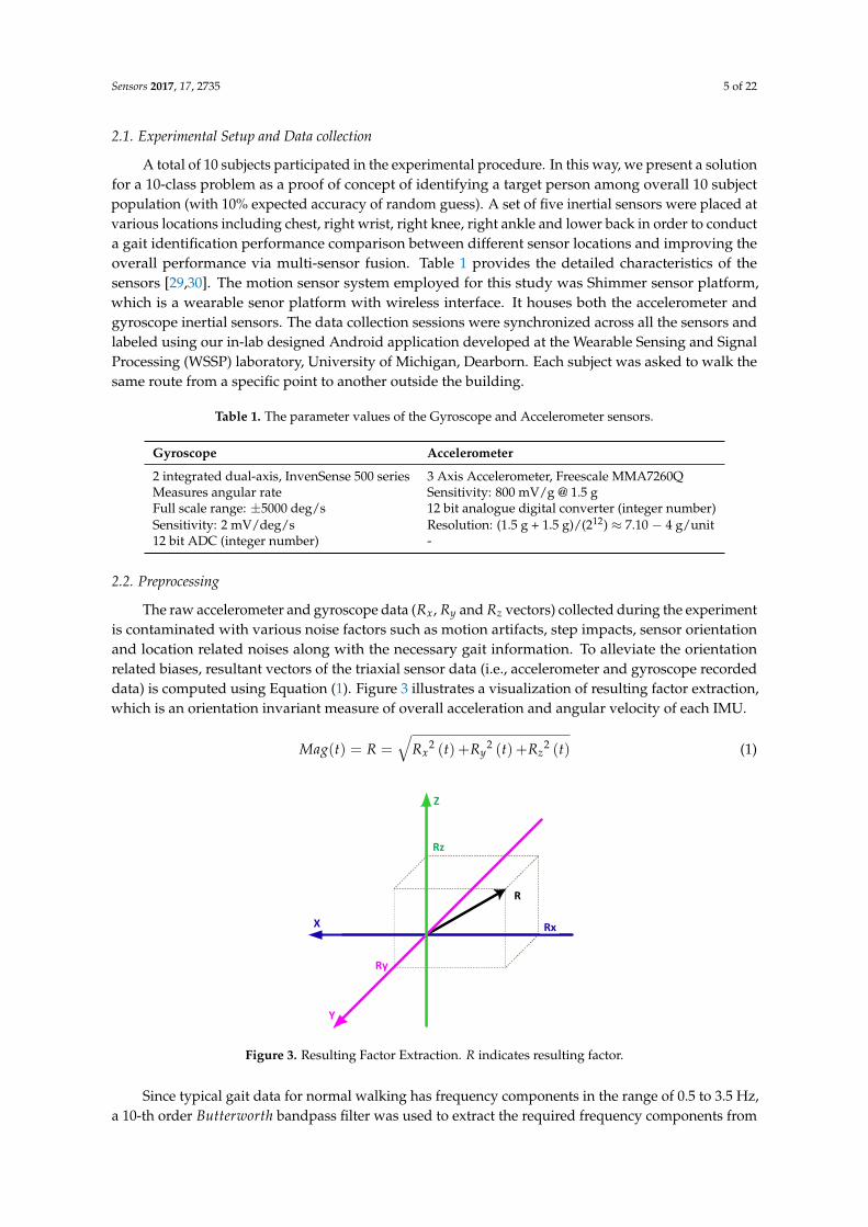
2.1. Experimental Setup and Data collection

A total of 10 subjects participated in the experimental procedure. In this way, we present a solutionfor a 10-class problem as a proof of concept of identifying a target person among overall 10 subjectpopulation (with 10% expected accuracy of random guess). A set of five inertial sensors were placed atvarious locations including chest, right wrist, right knee, right ankle and lower back in order to conducta gait identification performance comparison between different sensor locations and improving theoverall performance via multi-sensor fusion. Table 1 provides the detailed characteristics of thesensors [29,30]. The motion sensor system employed for this study was Shimmer sensor platform,which is a wearable senor platform with wireless interface. It houses both the accelerometer andgyroscope inertial sensors. The data collection sessions were synchronized across all the sensors andlabeled using our in-lab designed Android application developed at the Wearable Sensing and SignalProcessing (WSSP) laboratory, University of Michigan, Dearborn. Each subject was asked to walk thesame route from a specific point to another outside the building.

Table 1. The parameter values of the Gyroscope and Accelerometer sensors.

Gyroscope Accelerometer

2 integrated dual-axis, InvenSense 500 series 3 Axis Accelerometer, Freescale MMA7260QMeasures angular rate Sensitivity: 800 mV/g @ 1.5 gFull scale range: ±5000 deg/s 12 bit analogue digital converter (integer number)Sensitivity: 2 mV/deg/s Resolution: (1.5 g + 1.5 g)/(212) ≈ 7.10 − 4 g/unit12 bit ADC (integer number) -

2.2. Preprocessing

The raw accelerometer and gyroscope data (Rx, Ry and Rz vectors) collected during the experimentis contaminated with various noise factors such as motion artifacts, step impacts, sensor orientationand location related noises along with the necessary gait information. To alleviate the orientationrelated biases, resultant vectors of the triaxial sensor data (i.e., accelerometer and gyroscope recordeddata) is computed using Equation (1). Figure 3 illustrates a visualization of resulting factor extraction,which is an orientation invariant measure of overall acceleration and angular velocity of each IMU.

Mag(t) = R =√

Rx2 (t) +Ry

2 (t) +Rz2 (t) (1)

X Rx

Z

Rz

Ry

Y

R

Figure 3. Resulting Factor Extraction. R indicates resulting factor.

Since typical gait data for normal walking has frequency components in the range of 0.5 to 3.5 Hz,a 10-th order Butterworth bandpass filter was used to extract the required frequency components from

Sensors 2017, 17, 2735 6 of 22

the resultant vectors of the IMUs. For Gyroscope data, we assume the first estimated value of directionvectors to be the same as the direction vectors measured by the accelerometer:

RxEst(0) = Rx Acc(0)

RyEst(0) = Ry Acc(0)

RzEst(0) = Rz Acc(0)

(2)

In our algorithm, we assume the value of the accelerometer, when the sensor device is at rest(a first few seconds recordings before subjects started the gait paradigm), to be zero.

2.3. Gait Cycle Extraction

Since the data collection through all the sensors is time synchronized, we extracted the gait cyclesfrom the sensor#1 (i.e., the ankle sensor) and used the same markers for other sensors. The cycleextraction process implements amplitude check and zero crossing check to extract noise free gaitcycle data.

To approximate the gait cycle frequency, the resultant vectors of accelerometer data from sensor#1RAcc are passed through a band pass filter of rage 0.5–1.5 Hz. We conduct a more aggressive band passfiltering only for the purpose of cycle extraction. This eliminates the interference of any high frequencycomponents while determining the gait cycle frequency. The frequency range of 0.5–1.5 Hz is chosento include the average gait frequency, which is 1 Hz. Frequency Analysis consists of finding the energydistribution as a function of the frequency index ω. Therefore, it is necessary to transform the signal tothe frequency domain by means of the Fourier transformation:

X(ω) =∫

x(t)e−jtωdt (3)

where x(t) is the time domain signal. A Fourier transform is performed on the resultant data and thedominant frequency component within the range of 0.5 to 1.5 Hz is selected as the gait cycle frequencyof that subject fcycle.

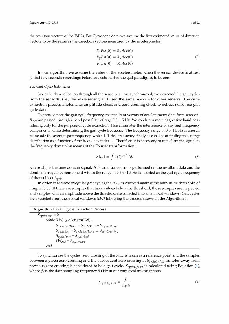
In order to remove irregular gait cycles,the RAcc is checked against the amplitude threshold ofa signal 0.05. If there are samples that have values below the threshold, those samples are neglectedand samples with an amplitude above the threshold are collected into small local windows. Gait cyclesare extracted from these local windows (LW) following the process shown in the Algorithm 1.

Algorithm 1: Gait Cycle Extraction ProcessScycleStart = 0

while (LWend < length(LW))ScycleEndTemp = ScycleStart + ScycleO f f setScycleEnd = ScycleEndTemp ± SzeroCrossingScycleStart = ScycleEndLWend = ScycleStart

end

To synchronize the cycles, zero crossing of the RAcc is taken as a reference point and the samplesbetween a given zero crossing and the subsequent zero crossing at ScycleO f f set samples away fromprevious zero crossing is considered to be a gait cycle. ScycleO f f set is calculated using Equation (4),where fs is the data sampling frequency 50 Hz in our empirical investigations.

ScycleO f f set =fs

fcycle(4)

Sensors 2017, 17, 2735 7 of 22

The end sample of this cycle ScycleEndTemp is approximated initially based on the fcycle but a moreprecise ScycleEnd is calculated based on finding a zero-crossing sample near the initial approximation.The local window indices of the start and end of cycle data ScycleStart and ScycleEnd are then mapped tothe global window of RAcc.

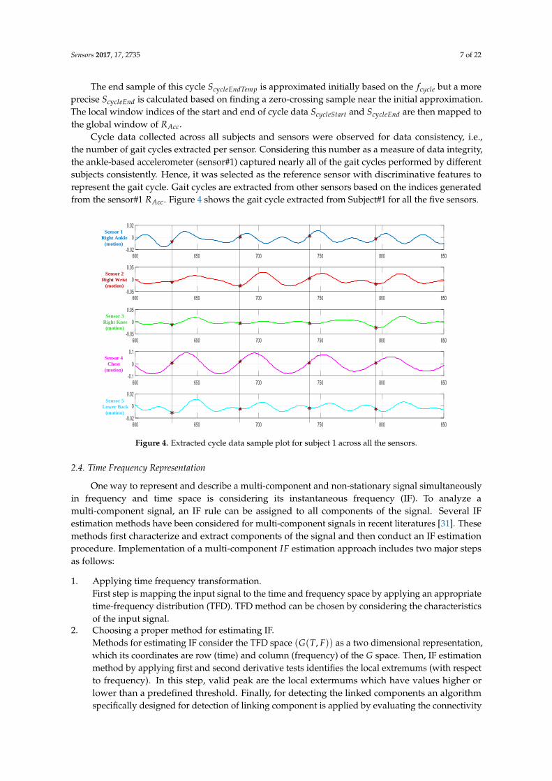
Cycle data collected across all subjects and sensors were observed for data consistency, i.e.,the number of gait cycles extracted per sensor. Considering this number as a measure of data integrity,the ankle-based accelerometer (sensor#1) captured nearly all of the gait cycles performed by differentsubjects consistently. Hence, it was selected as the reference sensor with discriminative features torepresent the gait cycle. Gait cycles are extracted from other sensors based on the indices generatedfrom the sensor#1 RAcc. Figure 4 shows the gait cycle extracted from Subject#1 for all the five sensors.

Sensor 5

Lower Back

(motion)

Sensor 1

Right Ankle

(motion)

Sensor 3

Right Knee

(motion)

Sensor 2

Right Wrist

(motion)

Sensor 4

Chest

(motion)

Figure 4. Extracted cycle data sample plot for subject 1 across all the sensors.

2.4. Time Frequency Representation

One way to represent and describe a multi-component and non-stationary signal simultaneouslyin frequency and time space is considering its instantaneous frequency (IF). To analyze amulti-component signal, an IF rule can be assigned to all components of the signal. Several IFestimation methods have been considered for multi-component signals in recent literatures [31]. Thesemethods first characterize and extract components of the signal and then conduct an IF estimationprocedure. Implementation of a multi-component IF estimation approach includes two major stepsas follows:

1. Applying time frequency transformation.First step is mapping the input signal to the time and frequency space by applying an appropriatetime-frequency distribution (TFD). TFD method can be chosen by considering the characteristicsof the input signal.

2. Choosing a proper method for estimating IF.Methods for estimating IF consider the TFD space (G(T, F)) as a two dimensional representation,which its coordinates are row (time) and column (frequency) of the G space. Then, IF estimationmethod by applying first and second derivative tests identifies the local extremums (with respectto frequency). In this step, valid peak are the local extermums which have values higher orlower than a predefined threshold. Finally, for detecting the linked components an algorithmspecifically designed for detection of linking component is applied by evaluating the connectivity

Sensors 2017, 17, 2735 8 of 22

of the pixels and also the number of the connected pixels. The fact behind this is that IF ofa component of a signal (where energy of the signal is concentrated) is observable in the TFDspace as a ridge which describes the IF.

Selection of a proper TFD representation approach for representing gait cycle can be countedas the first step in designing any identification system using TF space. A proper TFD method isthe one which is capable of emphasizing the non-stationarities of the given signal which, in turn,gives the system highest discriminative power to correctly discriminate between different cases in thepopulation under consideration. In this study we use smoothed Wigner-Ville distribution (SWVD)as it is capable of reducing the cross-term affection while it provides good resolution [31,32]. SWVDis a variant method which incorporates smoothing by independent windows in time and frequency,namely (τ) and (t):

SPWV(t, ω) =∫ +∞

−∞Wω(τ)[

∫ +∞

−∞Wt(u− t)x(u +

τ)

2x∗(u− τ

2)du]ejωτdτ (5)

The feature extraction using SWVD is based on Energy, Frequency and Length of the principaltrack. Each segment gives the values Ek (energy), Fk (frequency), and Lk (length). The signal is firstlydivided into segments; then, the construction of a three-dimensional feature vector for each segmentwill take place. Energy of each segment can be calculated as follows:

Ek =∫ ∫ +∞

−∞ϑk(t, f )dtd f (6)

where ϑk(t, f ) stands for the time-frequency representation of the segment. However, to calculate thefrequency of each segment k, we made use of the marginal frequency as follows:

Fk =∫ +∞

−∞ϑk(t, f )dt (7)

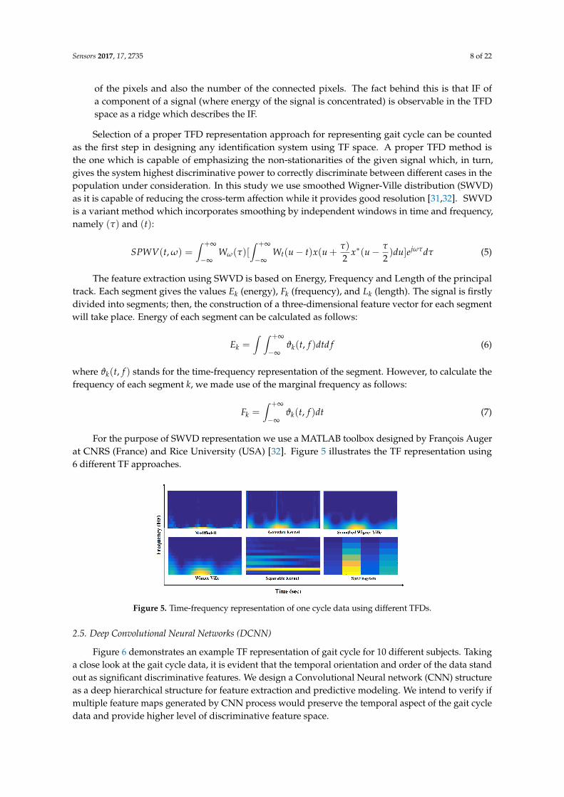
For the purpose of SWVD representation we use a MATLAB toolbox designed by François Augerat CNRS (France) and Rice University (USA) [32]. Figure 5 illustrates the TF representation using6 different TF approaches.

Figure 5. Time-frequency representation of one cycle data using different TFDs.

2.5. Deep Convolutional Neural Networks (DCNN)

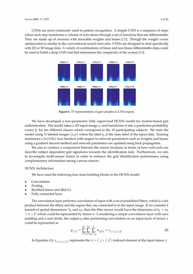
Figure 6 demonstrates an example TF representation of gait cycle for 10 different subjects. Takinga close look at the gait cycle data, it is evident that the temporal orientation and order of the data standout as significant discriminative features. We design a Convolutional Neural network (CNN) structureas a deep hierarchical structure for feature extraction and predictive modeling. We intend to verify ifmultiple feature maps generated by CNN process would preserve the temporal aspect of the gait cycledata and provide higher level of discriminative feature space.

Sensors 2017, 17, 2735 9 of 22

CNNs are most commonly used in pattern recognition. A simple CNN is a sequence of stepswhere each step transforms a volume of activations through a set of functions that are differentiable.They are made up of neurons with learnable weights and biases [33]. Though the weight vectoroptimization is similar to the conventional neural networks. CNNs are designed to deal specificallywith 2D or 3D image data. A variety of combinations of linear and non-linear differentiable steps couldbe used to build a deep CNN and that determines the complexity of the system [34].

Figure 6. TF representation of gait samples as CNN inputs.

We have developed a non-parametric fully supervised DCNN model for motion-based gaitauthentication. The model takes a 3D input image xi and transforms it into a prediction probabilityvector yi for ten different classes which correspond to the 10 participating subjects. We train themodel using N labeled images {x,y} where the label yi is the class label of the input data. Trainingminimizes a So f tMax loss function with respect to network parameters such as weights and biasesusing a gradient descent method and network parameters are updated using back propagation.

We aim to conduct a comparison between the sensor locations in terms of how well each candescribe subject dependent gait signatures towards the identification task. Furthermore, we aimto investigate multi-sensor fusion in order to enhance the gait identification performance usingcomplementary information among various sensors.

DCNN Architecture

We have used the following four main building blocks in the DCNN model:

• Convolution.• Pooling.• Rectified linear unit (ReLU).• Fully connected layer.

The convolution layer performs convolution of input with a set of predefined filters, which is a dotproduct between the filters and the region they are connected to in the input image. If we consider kkernels of spatial dimensions’ hk and wk, then the filter tensor would have the dimension of hk × wk× k × k′ which could be represented by tensor w. Considering a simple convolution layer with zeropadding and a unit stride, the output y after performing convolution on an input layer of tensor xcould be represented as

yi′ j′ k =hk

∑i=0

wk

∑j=0

k

∑k′=0

wijk′ k × xi+i′ ,j+j′ ,k′ (8)

In Equation (8), xi+i′ ,j+j′ ,k′ represents the (i + i′, j + j

′, k′) indexed element of the input tensor x.

Sensors 2017, 17, 2735 10 of 22

The pooling layer applies a chosen operator and combines closely associated feature values.It is used to down sample the input image along the width and height. This layer does not requireparameter learning. A simple implementation of max pooling can be represented as

yi′ j′ k =Max0 ≤i ≤hp , 0 ≤j ≤wp

{xi′∗ hp+i, j

′∗wp+j, k} (9)

where x and y represent the i′j′k indexed input and output layer and hp, wp are the pooling

window dimensions.The Rectified Linear Unit (ReLU) is a non-linear activation layer introduces the non-linearity

when applied to the feature map. ReLU layer leaves the size of its input unchanged. A simpleimplementation of ReLU would be as below:

yi′ j′ k= max{0,xi′ j′ k′ }. (10)

where x and y are input and output of corresponding tensors. Like pooling layer, ReLU does not needany parameter learning and it does not alter the dimensions of the input layer.

3. Multi-Sensor Fusion

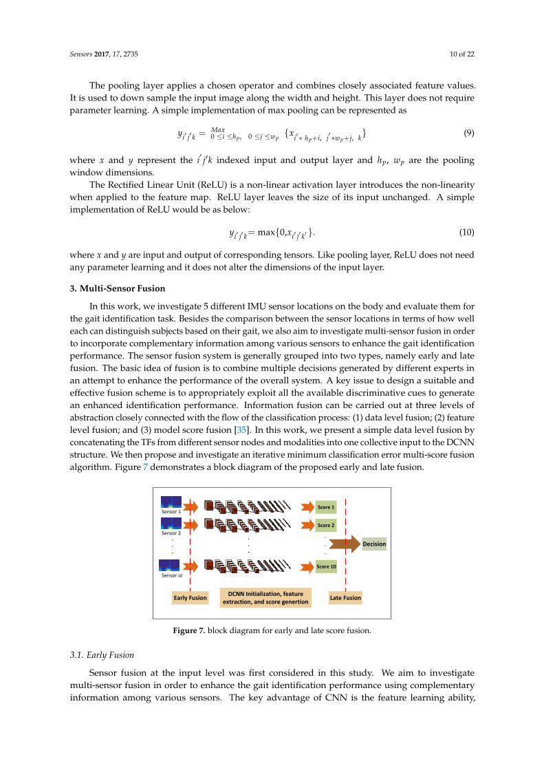
In this work, we investigate 5 different IMU sensor locations on the body and evaluate them forthe gait identification task. Besides the comparison between the sensor locations in terms of how welleach can distinguish subjects based on their gait, we also aim to investigate multi-sensor fusion in orderto incorporate complementary information among various sensors to enhance the gait identificationperformance. The sensor fusion system is generally grouped into two types, namely early and latefusion. The basic idea of fusion is to combine multiple decisions generated by different experts inan attempt to enhance the performance of the overall system. A key issue to design a suitable andeffective fusion scheme is to appropriately exploit all the available discriminative cues to generatean enhanced identification performance. Information fusion can be carried out at three levels ofabstraction closely connected with the flow of the classification process: (1) data level fusion; (2) featurelevel fusion; and (3) model score fusion [35]. In this work, we present a simple data level fusion byconcatenating the TFs from different sensor nodes and modalities into one collective input to the DCNNstructure. We then propose and investigate an iterative minimum classification error multi-score fusionalgorithm. Figure 7 demonstrates a block diagram of the proposed early and late fusion.

.

.

.

Score 1

Score 2

Score 10

.

.

.

Early Fusion Late FusionDCNN Initialization, feature

extraction, and score genertion

Sensor 1

Sensor 2

Sensor 10

Decision...

Figure 7. block diagram for early and late score fusion.

3.1. Early Fusion

Sensor fusion at the input level was first considered in this study. We aim to investigatemulti-sensor fusion in order to enhance the gait identification performance using complementaryinformation among various sensors. The key advantage of CNN is the feature learning ability,

Sensors 2017, 17, 2735 11 of 22

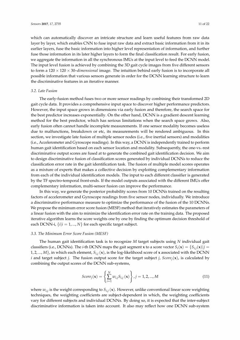
which can automatically discover an intricate structure and learn useful features from raw datalayer by layer, which enables CNN to fuse input raw data and extract basic information from it in itsearlier layers, fuse the basic information into higher level representation of information, and furtherfuse those information in its later higher layers to form the final classification result. For early fusion,we aggregate the information in all the synchronous IMUs at the input level to feed the DCNN model.The input level fusion is achieved by combining the 3D gait cycle images from five different sensorsto form a 120× 120× 30–dimensional image. The intuition behind early fusion is to incorporate allpossible information that various sensors generate in order for the DCNN learning structure to learnthe discriminative features in an iterative manner.

3.2. Late Fusion

The early-fusion method fuses two or more sensor readings by combining their transformed 2Dgait cycle data. It provides a comprehensive input space to discover higher performance predictors.However, the input space grows in dimensions via early fusion and therefore, the search space forthe best predictor increases exponentially. On the other hand, DCNN is a gradient descent learningmethod for the best predictor, which has serious limitations when the search space grows. Also,early fusion often cannot handle incomplete measurements. If one sensor modality becomes uselessdue to malfunctions, breakdown or etc, its measurements will be rendered ambiguous. In thissection, we investigate late fusion of multiple sensor nodes (i.e., five inertial sensors) and modalities(i.e., Accelerometer and Gyroscope readings). In this way, a DCNN is independently trained to performhuman gait identification based on each sensor location and modality. Subsequently, the one-vs.-restdiscriminative output scores are fused at to generate the combined gait identification decision. We aimto design discriminative fusion of classification scores generated by individual DCNNs to reduce theclassification error rate in the gait identification task. The fusion of multiple model scores operatesas a mixture of experts that makes a collective decision by exploiting complementary informationfrom each of the individual identification models. The input to each different classifier is generatedby the TF spectro-temporal front-ends. If the model outputs associated with the different IMUs offercomplementary information, multi-sensor fusion can improve the performance.

In this way, we generate the posterior probability scores from 10 DCNNs trained on the resultingfactors of accelerometer and Gyroscope readings from five sensor nodes, individually. We introducea discriminative performance measure to optimize the performance of the fusion of the 10 DCNNs.We propose the minimum error score fusion (MESF) method that iteratively estimates the parameters ofa linear fusion with the aim to minimize the identification error rate on the training data. The proposediterative algorithm learns the score weights one by one by finding the optimum decision threshold ofeach DCNN-i, {i|i = 1, ..., N} for each specific target subject.

3.3. The Minimum Error Score Fusion (MESF)

The human gait identification task is to recognize M target subjects using N individual gaitclassifiers (i.e., DCNNs). The i-th DCNN maps the gait segment x to a score vector Si(x) = {Si,j(x)|j =1, 2, ..., M}, in which each element, Si,j (x), is the log-likelihood score of x associated with the DCNNi and target subject j. The fusion output score for the target subject j, Scorej(x), is calculated bycombining the output scores of the DCNN sub-systems,

Scorej(x) =

{N

∑i=1

wi,jSi,j (x)

}, j = 1, 2, ..., M (11)

where wi,j is the weight corresponding to Si,j (x). However, unlike conventional linear score weightingtechniques, the weighting coefficients are subject-dependent in which, the weighting coefficientsvary for different subjects and individual DCNNs. By doing so, it is expected that the inter-subjectdiscriminative information is taken into account. It also may reflect how one DCNN sub-system

Sensors 2017, 17, 2735 12 of 22

contributes to identify each particular subject. There are a total of N ×M weighting coefficients asfusion parameters to be estimated using the MESF algorithm. We then apply a normalization processon the scores of M target subjects.

3.3.1. The Process of Score Fusion

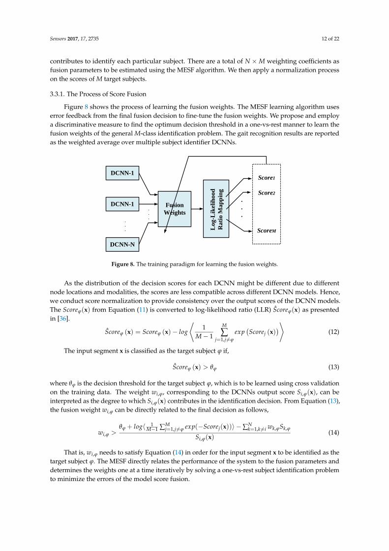
Figure 8 shows the process of learning the fusion weights. The MESF learning algorithm useserror feedback from the final fusion decision to fine-tune the fusion weights. We propose and employa discriminative measure to find the optimum decision threshold in a one-vs-rest manner to learn thefusion weights of the general M-class identification problem. The gait recognition results are reportedas the weighted average over multiple subject identifier DCNNs.

.

.

..

.

.

DCNN-1

DCNN-1

DCNN-N

Fusion

Weights L

og-L

ikeli

hood

Rati

o M

ap

pin

g

Score1

Score2

ScoreM

.

.

.

Figure 8. The training paradigm for learning the fusion weights.

As the distribution of the decision scores for each DCNN might be different due to differentnode locations and modalities, the scores are less compatible across different DCNN models. Hence,we conduct score normalization to provide consistency over the output scores of the DCNN models.The Scoreϕ(x) from Equation (11) is converted to log-likelihood ratio (LLR) Scoreϕ(x) as presentedin [36].

Scoreϕ (x) = Scoreϕ (x)− log

⟨1

M− 1

M

∑j=1,j 6=ϕ

exp(Scorej (x)

)⟩(12)

The input segment x is classified as the target subject ϕ if,

Scoreϕ (x) > θϕ (13)

where θϕ is the decision threshold for the target subject ϕ, which is to be learned using cross validationon the training data. The weight wi,ϕ, corresponding to the DCNNs output score Si,ϕ(x), can beinterpreted as the degree to which Si,ϕ(x) contributes in the identification decision. From Equation (13),the fusion weight wi,ϕ can be directly related to the final decision as follows,

wi,ϕ >θϕ + log〈 1

M−1 ∑Mj=1,j 6=ϕ exp(−Scorej(x))〉 −∑N

k=1,k 6=i wk,ϕSk,ϕ

Si,ϕ(x)(14)

That is, wi,ϕ needs to satisfy Equation (14) in order for the input segment x to be identified as thetarget subject ϕ. The MESF directly relates the performance of the system to the fusion parameters anddetermines the weights one at a time iteratively by solving a one-vs-rest subject identification problemto minimize the errors of the model score fusion.

Sensors 2017, 17, 2735 13 of 22

3.3.2. The MESF Algorithm for Fusion Weight Learning

(1) Discriminative performance measure of the linear fusion:

DCNN models usually assign a score S (x) to each unseen gait segment x, expressing the degree towhich x would belong to each of the subject classes. Ideally, the score is an accurate estimate of posteriorprobability distributions over the target subject class (i.e., positive class), p(′pos′|x), and the rest of thesubjects (i.e., negative class), p(′neg′|x), for an input x which denotes the estimated probabilities that xbelongs to the positive and negative classes, respectively. We introduce a measure, Θ(x) to convert theprobabilities into discriminative scores as below:

Θ(x) =p(′neg′|x)p(′pos′|x) (15)

The measure Θ(x) demonstrates the the degree to which x is predicted to be of the negative class).By optimizing a threshold on the Θ measure, a statistical classifier can be converted to a discriminativeclassifier. In this way, the input x is classified as negative if the Θ(x) is greater than a specified thresholdand positive otherwise. The desired threshold is learned by minimizing the classification error rate onthe training data.

(2) Minimum error rate decision threshold in one-vs.-rest manner:

Assume that a training set {(xt, yt)|t = 1, 2, ..., n} consisting of n labeled data and their Θ measureΘ(xt) is available. Using the training data, we aim to design an algorithm that finds the value ofthe linear fusion weight parameter that makes the optimum decision on a set of labeled trainingdata samples. The proposed algorithm aims to return the decision threshold ’optimum_thresh’ thatminimizes the error rate of the linear classifier fusion by varying the threshold value from 0 to +∞and find the optimum value by including false negatives (FN) in the positive class. Therefore, werank the data samples in an ascending order of their Θ(.) measure Θ(x1), ..., Θ(xP+N). Consideringany threshold, th, between Θ(xt) and Θ(xt+1), the first K data samples will be classified as positive,where Θ(xK) < th, and the remaining P + N − K data samples as negative. In this way, a maximum ofP + N + 1 different thresholds has to be examined to find the optimum decision threshold. The firstthreshold classifies everything as negative and the rest of the thresholds are chosen in the middle oftwo successive Θ measures.

The threshold, optimum_thresh, on the Θ(.) measure is found such that it minimizes the error rateof the DCNN model score fusion.The data sample xt is classified as positive if Θ(xt) ≤ optimum_thresh.That is, xt is classified as ′pos′ if,

p(x|′neg′)p(x|′pos′)

< optimum_thresh → p(x|′neg′) < optimum_thresh× p(x|′pos′) (16)

The algorithm results in the highest accuracy achievable with the given Θ(.) on the given set ofdata samples. In practice, the quality of the optimization depends on the quality of the positive andnegative scores, e.g., the output posterior probability distributions of the DCNN models. In our fusiontask, if the individual DCNN models generate good quality estimates, the fusion weight learning canconsiderably improve the performance. It can also be implemented in an efficient way by exploitingthe monotonically ranked Θ measures.

(3) Discriminative learning of the fusion score weights

We propose an iterative learning procedure in order to minimize the error of the overall humanidentifier in one-vs-rest manner by re-estimating the weight parameters of the model score fusion.The proposed learning method adjusts the fusion weights in the interval [0,∞) using the training gaitsegments. The weights assigned to the output scores Si,j(.) are set to one, for wi,j ← 1 for i = 1, ..., N,and j = 1, ..., M, as an initial solution to the problem. Then, the following procedure is presented,

Sensors 2017, 17, 2735 14 of 22

in which the error rate of the DCNN model fusion is successively reduced by finding a better solutionthan the current one by learning the locally optimum fusion weights, one at a time. To find the weightwi,ϕ, corresponding to the output score of the DCNN i for target subject ϕ, the problem is consideredto be a 2-class problem where the target subject ϕ is the positive class and ϕ comprising the rest of thesubjects is the negative class. The steps are as follows:

1. The wi,ϕ is set to zero, i.e., Si,ϕ(.) does not contribute in classification decision.2. The gait segments in the training set belonging to the subject ϕ that are classified correctly with

current values of the model score weights are marked. Adjusting the weight wi,ϕ does not haveany impact on their classification.

3. The gait segments of ϕ in the training set that are misclassified are marked. Adjusting the weightwi,ϕ does not have any impact on their classification.

4. The remaining m gait segments in the training set {xt|t = 1, ..., m} that are left unmarked are usedto determine wi,ϕ so that the error of the model score fusion is minimized over {xt|t = 1, ..., m}.From Equation (14), the measure Θi,ϕ(.) is calculated for every segment in {xt|t = 1, ..., m}as follows:

Θi,ϕ(xt) = [θϕ + log〈 1M− 1

M

∑j=1,j 6=ϕ

exp(−Scorej(xt))〉 −N

∑k=1,k 6=i

wk,ϕSk,ϕ(xt)]/Si,ϕ(xt) (17)

where, Θi,ϕ (xt) is the amount of wi,ϕ necessary for xt to be classified as the target subject ϕ.5. The training segments are ranked in an ascending order by their Θi,ϕ(.) measure. A threshold is

defined and initialized to zero. Then, assuming that xt and xt+1 are two successive segments inthe list, the threshold is computed as,

thresh = [Θi,ϕ(xt) + Θi,ϕ(xt+1)]/2 (18)

Then, the threshold is adjusted from the lowest score to the highest. For each threshold,the associated accuracy of the score fusion is measured. The value of the optimum_thresh leadingto the maximum accuracy is used as the estimated score weight wi,ϕ, assuming that all other scoreweights are fixed.

Figure 9 shows a data sample of a resulting threshold on the Θq,w(.) measure leading to thehighest accuracy. In this way, the input xt is classified as w if its Θ(xt) is lower than the threshold.The algorithm determines the optimal value of the parameter φq,w assuming that all other parametersare given and fixed.

xt belonging to the class ‘pos’

Training Instances xt

neg_odds (xt)

best_thresh

0.250.390.640.730.891.04

2.131.761.58

2.18

1.32

9.275.833.53

xt belonging to the class ‘neg’

Figure 9. A data sample of the resulting thresholds on the Θq,w(.) measure.

Sensors 2017, 17, 2735 15 of 22

The search for the locally optimum combination of weights is conducted by optimizing the scoreweights one at a time and learning stops if no improvement to the current performance can be made.Based on our observations, the above method consistently generated superior results. The MESFmethod determines the decision score weights of the sub-systems in order to better discriminatebetween the gait segments from subjects ϕ and those of the rest by finding the optimum decisionthreshold of the score fusion in the one-vs-rest manner. By doing so, we can interpret that the ROCcurve of the score fusion is locally optimized. As shown below, it is illustrated that the error rate onthe training data always reduces during the optimization and will converge to a minimum point.

ErrorRate(Λ ∪Φnewq,w , D) ≤ ErrorRate(Λ ∪Φold

q,w, D) (19)

where Λ is the set of all other parameters (Given & Fixed)

⇒ ErrorRate(Λ ∪Φtq,w, D) ≤ ErrorRate(Λ ∪Φt−1

q−1,w, D) ≥ ErrorRate(Λ ∪Φt−2q−2,w, D) ≤ ... (20)

where t represent the iteration number starting from 1 and increment after each learning iteration.After each iteration, the accuracy of the learning algorithm decreases.

3.4. Comparable Score Fusion Methods

In this section, some other linear score fusion methods are described for comparison. Assumean input gait segment x, and the output decision scores of the sub-systems, {Si,j(x)|i = 1, ..., N & j =1, ..., M} are available. Comparative methods include a simple non-trainable combiner and the largemargin method that require a more sophisticated training procedures.

• Summation: The output scores of the individual DCNNs are summed up and the subject thatreceives the highest score is the output decision of the fusion system.

Scoresumj (x) =

N

∑i=1

Si,j (x) (21)

• Support vector machine (SVM): SVM has shown to be effective in separating input vectors in2-class problems [37], in which SVM effectively projects the vector x into a scalar value f (x),

f (x) =N

∑i=1

αiyi (xi.x) + d (22)

where the vectors xi are support vectors, yi = {−1, 1} are the correct outputs, N is the number ofsupport vectors, (.) is the dot product function, αi are adjustable weights, and d is a bias. Learningis posed as an optimization problem with the goal of maximizing the margin, which is the distancebetween the separating hyperplane and the nearest training vectors. As a combiner method,the output scores of all the DCNNs are concatenated to form a vector as the input to SVMs. Then,one SVM is assigned to each of the M target subjects, the one-vs-rest scheme, and train accordinglyto get the final output scores,

ScoreSVMj (x) =

N

∑i=1

αiyi (φ (xi) .φ (x)) + d (23)

where φ(x) is the vector resulted by concatenating the output scores of all the DCNNs for theinput segment x.

Sensors 2017, 17, 2735 16 of 22

4. Results

We implemented a Matlab TF representation toolbox [38] to generate the SWVD TF representationof the data and use Matlab print function to output a 2D image with specific resolution and size.After experimenting with multiple image sizes, it was observed that higher image resolution did notnecessarily mean better model performance. DCNN model was tested with different input imagesizes. The image size was modified by changing the resolution of the figure generated by Matlabprint function. It was observed that the model prediction accuracies are highest with the image size of120× 120× 3 for our current analysis.

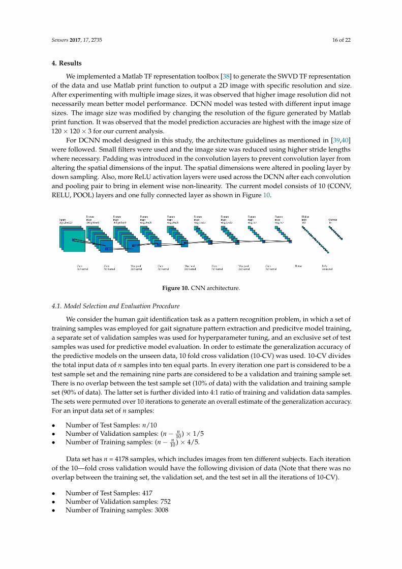
For DCNN model designed in this study, the architecture guidelines as mentioned in [39,40]were followed. Small filters were used and the image size was reduced using higher stride lengthswhere necessary. Padding was introduced in the convolution layers to prevent convolution layer fromaltering the spatial dimensions of the input. The spatial dimensions were altered in pooling layer bydown sampling. Also, more ReLU activation layers were used across the DCNN after each convolutionand pooling pair to bring in element wise non-linearity. The current model consists of 10 (CONV,RELU, POOL) layers and one fully connected layer as shown in Figure 10.

Figure 10. CNN architecture.

4.1. Model Selection and Evaluation Procedure

We consider the human gait identification task as a pattern recognition problem, in which a set oftraining samples was employed for gait signature pattern extraction and predicitve model training,a separate set of validation samples was used for hyperparameter tuning, and an exclusive set of testsamples was used for predictive model evaluation. In order to estimate the generalization accuracy ofthe predictive models on the unseen data, 10 fold cross validation (10-CV) was used. 10-CV dividesthe total input data of n samples into ten equal parts. In every iteration one part is considered to be atest sample set and the remaining nine parts are considered to be a validation and training sample set.There is no overlap between the test sample set (10% of data) with the validation and training sampleset (90% of data). The latter set is further divided into 4:1 ratio of training and validation data samples.The sets were permuted over 10 iterations to generate an overall estimate of the generalization accuracy.For an input data set of n samples:

• Number of Test Samples: n/10• Number of Validation samples: (n− n

10 ) × 1/5• Number of Training samples: (n− n

10 ) × 4/5.

Data set has n = 4178 samples, which includes images from ten different subjects. Each iterationof the 10—fold cross validation would have the following division of data (Note that there was nooverlap between the training set, the validation set, and the test set in all the iterations of 10-CV).

• Number of Test Samples: 417• Number of Validation samples: 752• Number of Training samples: 3008

Sensors 2017, 17, 2735 17 of 22

Figure 6, shows a sample image set of all subjects for sensor#1. The DCNN model was trainedusing the training and validation set and tested independently with the testing set. In order to fine-tunethe parameters of the DCNN model, we conducted random restart hill climbing search method ona low resolution quantized parameter space to achieve a reliable local minimum in the error function(i.e., the average error rate of the model on the 5 individual sensor locations). Table 2 reports theselected parameters to train the gait identification DCNN models. It must be noted that no of epochswas set to 19 since, we terminate training at 19 epochs where we get maximum accuracy and the modelis able to generalize enough and avoids overfitting.

Table 2. CNN predefined parameters.

Parameter Values

Learning Rate 0.001Momentum Coefficient 0.9

No. of Feature Maps 32, 64No. of Neurons in Fully Connected Layer 64

Batch Size 40Epoch Number 19Epoch Number 19

4.2. Individual Sensor Performance

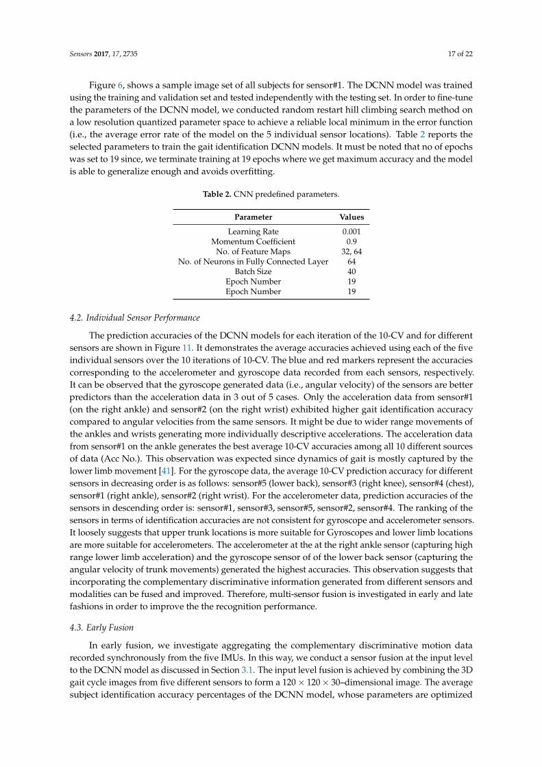
The prediction accuracies of the DCNN models for each iteration of the 10-CV and for differentsensors are shown in Figure 11. It demonstrates the average accuracies achieved using each of the fiveindividual sensors over the 10 iterations of 10-CV. The blue and red markers represent the accuraciescorresponding to the accelerometer and gyroscope data recorded from each sensors, respectively.It can be observed that the gyroscope generated data (i.e., angular velocity) of the sensors are betterpredictors than the acceleration data in 3 out of 5 cases. Only the acceleration data from sensor#1(on the right ankle) and sensor#2 (on the right wrist) exhibited higher gait identification accuracycompared to angular velocities from the same sensors. It might be due to wider range movements ofthe ankles and wrists generating more individually descriptive accelerations. The acceleration datafrom sensor#1 on the ankle generates the best average 10-CV accuracies among all 10 different sourcesof data (Acc No.). This observation was expected since dynamics of gait is mostly captured by thelower limb movement [41]. For the gyroscope data, the average 10-CV prediction accuracy for differentsensors in decreasing order is as follows: sensor#5 (lower back), sensor#3 (right knee), sensor#4 (chest),sensor#1 (right ankle), sensor#2 (right wrist). For the accelerometer data, prediction accuracies of thesensors in descending order is: sensor#1, sensor#3, sensor#5, sensor#2, sensor#4. The ranking of thesensors in terms of identification accuracies are not consistent for gyroscope and accelerometer sensors.It loosely suggests that upper trunk locations is more suitable for Gyroscopes and lower limb locationsare more suitable for accelerometers. The accelerometer at the at the right ankle sensor (capturing highrange lower limb acceleration) and the gyroscope sensor of of the lower back sensor (capturing theangular velocity of trunk movements) generated the highest accuracies. This observation suggests thatincorporating the complementary discriminative information generated from different sensors andmodalities can be fused and improved. Therefore, multi-sensor fusion is investigated in early and latefashions in order to improve the the recognition performance.

4.3. Early Fusion

In early fusion, we investigate aggregating the complementary discriminative motion datarecorded synchronously from the five IMUs. In this way, we conduct a sensor fusion at the input levelto the DCNN model as discussed in Section 3.1. The input level fusion is achieved by combining the 3Dgait cycle images from five different sensors to form a 120× 120× 30–dimensional image. The averagesubject identification accuracy percentages of the DCNN model, whose parameters are optimized

Sensors 2017, 17, 2735 18 of 22

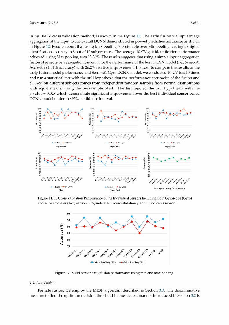
using 10-CV cross validation method, is shown in the Figure 12. The early fusion via input imageaggregation at the input to one overall DCNN demonstrated improved prediction accuracies as shownin Figure 12. Results report that using Max pooling is preferable over Min pooling leading to higheridentification accuracy in 8 out of 10 subject cases. The average 10-CV gait identification performanceachieved, using Max pooling, was 93.36%. The results suggests that using a simple input aggregationfusion of sensors by aggregation can enhance the performance of the best DCNN model (i.e., Sensor#1Acc with 91.01% accuracy) with 26.2% relative improvement. In order to compare the results of theearly fusion model performance and Sensor#1 Gyro DCNN model, we conducted 10-CV test 10 timesand run a statistical test with the null hypothesis that the performance accuracies of the fusion and’S1 Acc’ on different subjects comes from independent random samples from normal distributionswith equal means, using the two-sample t-test. The test rejected the null hypothesis with thep-value = 0.028 which demonstrate significant improvement over the best individual sensor-basedDCNN model under the 95% confidence interval.

50

55

60

65

70

75

80

85

90

95

100

S1 Acc S1 Gyro

50

55

60

65

70

75

80

85

90

95

100

S2 Acc S2 Gyro

50

55

60

65

70

75

80

85

90

95

100

S3 Acc S3 Gyro

50556065707580859095

100

S4 Acc S4 Gyro

50556065707580859095

100

S5 Acc S5 GyroAverage accuracy for 10 sensors

Acc

ura

cy (

%)

Acc

ura

cy (

%)

Acc

ura

cy (

%)

Acc

ura

cy (

%)

Acc

ura

cy (

%)

Acc

ura

cy (

%)

50556065707580859095

100

Right Ankle Right Wrist Right Knee

Chest Lower Back

Figure 11. 10 Cross Validation Performance of the Individual Sensors Including Both Gyroscope (Gyro)and Accelerometer (Acc) sensors. CVj indicates Cross-Validation j, and Si indicates sensor i.

Acc

ura

cy (

%)

75

80

85

90

95

100

Max Pooling (%) Min Pooling (%)

Figure 12. Multi-sensor early fusion performance using min and max pooling.

4.4. Late Fusion

For late fusion, we employ the MESF algorithm described in Section 3.3. The discriminativemeasure to find the optimum decision threshold in one-vs-rest manner introduced in Section 3.2 is

Sensors 2017, 17, 2735 19 of 22

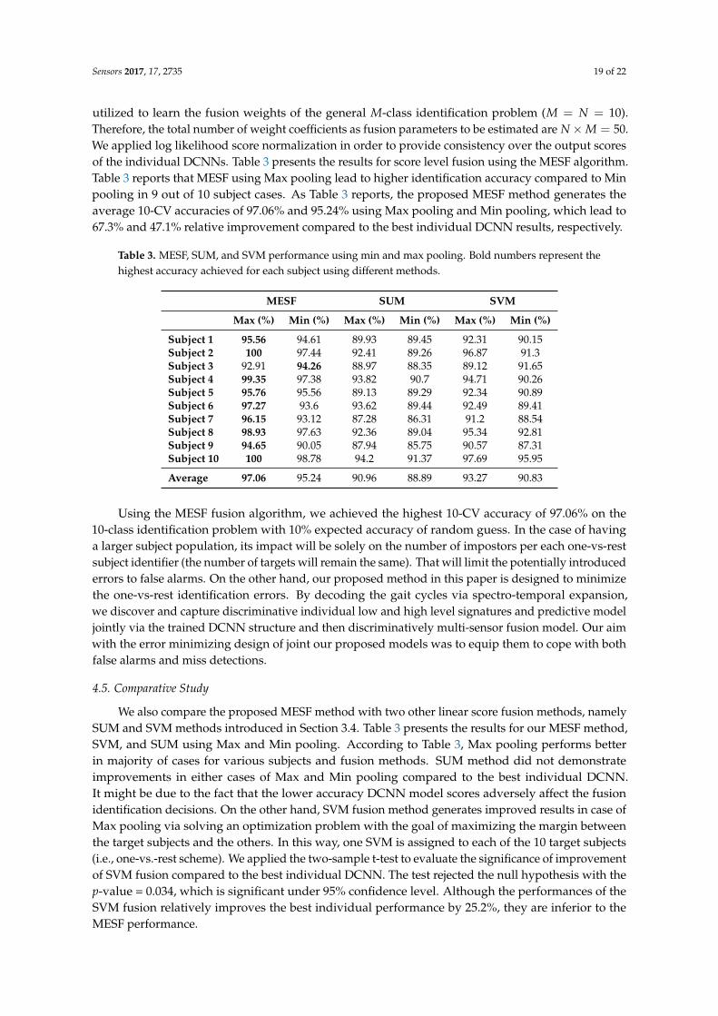
utilized to learn the fusion weights of the general M-class identification problem (M = N = 10).Therefore, the total number of weight coefficients as fusion parameters to be estimated are N×M = 50.We applied log likelihood score normalization in order to provide consistency over the output scoresof the individual DCNNs. Table 3 presents the results for score level fusion using the MESF algorithm.Table 3 reports that MESF using Max pooling lead to higher identification accuracy compared to Minpooling in 9 out of 10 subject cases. As Table 3 reports, the proposed MESF method generates theaverage 10-CV accuracies of 97.06% and 95.24% using Max pooling and Min pooling, which lead to67.3% and 47.1% relative improvement compared to the best individual DCNN results, respectively.

Table 3. MESF, SUM, and SVM performance using min and max pooling. Bold numbers represent thehighest accuracy achieved for each subject using different methods.

MESF SUM SVM

Max (%) Min (%) Max (%) Min (%) Max (%) Min (%)

Subject 1 95.56 94.61 89.93 89.45 92.31 90.15Subject 2 100 97.44 92.41 89.26 96.87 91.3Subject 3 92.91 94.26 88.97 88.35 89.12 91.65Subject 4 99.35 97.38 93.82 90.7 94.71 90.26Subject 5 95.76 95.56 89.13 89.29 92.34 90.89Subject 6 97.27 93.6 93.62 89.44 92.49 89.41Subject 7 96.15 93.12 87.28 86.31 91.2 88.54Subject 8 98.93 97.63 92.36 89.04 95.34 92.81Subject 9 94.65 90.05 87.94 85.75 90.57 87.31Subject 10 100 98.78 94.2 91.37 97.69 95.95

Average 97.06 95.24 90.96 88.89 93.27 90.83

Using the MESF fusion algorithm, we achieved the highest 10-CV accuracy of 97.06% on the10-class identification problem with 10% expected accuracy of random guess. In the case of havinga larger subject population, its impact will be solely on the number of impostors per each one-vs-restsubject identifier (the number of targets will remain the same). That will limit the potentially introducederrors to false alarms. On the other hand, our proposed method in this paper is designed to minimizethe one-vs-rest identification errors. By decoding the gait cycles via spectro-temporal expansion,we discover and capture discriminative individual low and high level signatures and predictive modeljointly via the trained DCNN structure and then discriminatively multi-sensor fusion model. Our aimwith the error minimizing design of joint our proposed models was to equip them to cope with bothfalse alarms and miss detections.

4.5. Comparative Study

We also compare the proposed MESF method with two other linear score fusion methods, namelySUM and SVM methods introduced in Section 3.4. Table 3 presents the results for our MESF method,SVM, and SUM using Max and Min pooling. According to Table 3, Max pooling performs betterin majority of cases for various subjects and fusion methods. SUM method did not demonstrateimprovements in either cases of Max and Min pooling compared to the best individual DCNN.It might be due to the fact that the lower accuracy DCNN model scores adversely affect the fusionidentification decisions. On the other hand, SVM fusion method generates improved results in case ofMax pooling via solving an optimization problem with the goal of maximizing the margin betweenthe target subjects and the others. In this way, one SVM is assigned to each of the 10 target subjects(i.e., one-vs.-rest scheme). We applied the two-sample t-test to evaluate the significance of improvementof SVM fusion compared to the best individual DCNN. The test rejected the null hypothesis with thep-value = 0.034, which is significant under 95% confidence level. Although the performances of theSVM fusion relatively improves the best individual performance by 25.2%, they are inferior to theMESF performance.

Sensors 2017, 17, 2735 20 of 22

5. Conclusions

In the human gait recognition task, the aim is to extract discriminative features and descriptorsfrom gait motion signals to identify our target subject from others. The manual feature extractionis prone to error due to the complexity of data collected from inertial sensors and the disconnectionbetween feature extraction and the discriminative learning models. To overcome this shortcoming,we proposed a novel methodology for processing non-stationary signals for the purpose of humangait identification. The proposed methodology comprises four main components: (1) cycleextraction; (2) spectro-temporal 2D expansion and representation; (3) deep convolutional learning;and (4) discriminative multi-sensor model score fusion. We first isolated the gait cycles using a simpleand effective heuristic. Then, we conducted spectro-temporal transformation of isolated gait cycles.The 2-D expansion of the gait cycle increased the resolution of the desired discriminative trends in thejoint time-frequency domain. In order to avoid manual feature extraction and incorporate joint featureand model learning from the generated high resolution 2D data, we designed a deep convolutionalneural network structure in order to process the signal layer by layer, extract discriminative features,and jointly optimize the features and the predictive model via error back propagation model training.We investigated 5 IMU sensor placement on the body and conducted a comparative investigationbetween them in terms of gait identification performance using synchronized gait data recordingsfrom 10 subjects. Due to complementary discriminative signature patterns captured from the recordedsignals collected via different sensors, we then investigated gait identification fusion modeling frommulti-node inertial sensor data and effectively expand it via 2-D time-frequency transformation.We perform early (input level) and late (model score level) multi-sensor fusion to improve thecross validation accuracy of the gait identification task. We particularly proposed the minimumerror DCNN model score fusion algorithm. Based on our experimental results, 93.88% and 97.06%subject identification accuracy was achieved via early and late fusion of the multi-node sensorreadings, respectively.

6. Future Research Direction

In this paper, the problem of human gait identification was investigated under the bigger umbrellaof ubiquitous and continuous IMU-based gait analysis work group at the Wearable Sensing and SignalProcessing (WSSP) lab. Our main contribution and focus in this paper was our proposed model scorefusion algorithm to incorporate the complementary discriminative scores generated by each individualDCNN model given a input human gait cycles. We used a local search and an overall accuracy togenerate a reliable baseline DCNN model for all the IMU recordings. Due to the fact that data fromdifferent sensors (i.e., sources) may have different characteristics, the DCNN training paradigm canbe improved by sensor-dependent tuning for different sensor locations and modalities. Therefore,our team is currently investigating sensor location and modality specific DCNN model optimizationand subsequently, designing multi-sensor and multi-model fusion algorithms. We are also increasingthe number of subjects and the walking conditions in our data set. When completed, our plan is tocreate a link on our website to share our data set and our baseline model implementations with theresearch community.

Acknowledgments: The authors gratefully acknowledge financial support from Ford smart mobility center.

Author Contributions: Omid contributed in concept of the study, CNN architecture design and discriminativefusion algorithm, writing and preparing the manuscript. Mojtaba contributed in data analytics andtime—frequency representation, CNN design and result generation, and writing and preparing the manuscript.Raghavendar contributed in gait cycle extraction, conducting CNN and fusion result generation.

Conflicts of Interest: The authors declare no conflict of interest.

References

1. Murray, M.; Pat, A.; Bernard, D.; Ross, C.K. Walking patterns of normal men. JBJS 1964, 46, 335–360.

Sensors 2017, 17, 2735 21 of 22

2. Jellinger, K.; Armstrong, D.; Zoghbi, H.Y.; Percy, A.K. Neuropathology of Rett syndrome. Acta Neuropathol.1988, 76, 142–158.

3. Katz, J.N.; Dalgas, M.; Stucki, G. Degenerative lumbar spinal stenosis Diagnostic value of the history andphysical examination. Arthritis Rheumatol. 1995, 38, 1236–1241.

4. Nutt, J.G.; Marsden, C.D.; Thompson, P.D. Human walking and higher-level gait disorders, particularly inthe elderly. Neurology 1993, 43, 268.

5. El-Sheimy, N.; Haiying, H.; Xiaoji, N. Analysis and modeling of inertial sensors using Allan variance.IEEE Trans. Instrum. Meas. 2008, 57, 140–149.

6. Kale, A.; Sundaresan, A.; Rajagopalan, A.N.; Cuntoor, N.P.; Roy-Chowdhury, A.K.; Krüger, V.; Chellappa, R.Identification of humans using gait. IEEE Trans. Image Process. 2004, 13, 1163–1173.

7. Sprager, S.; Matjaz, B.J. Inertial sensor-based gait recognition: A review. Sensors 2015, 15, 22089–22127.8. Gafurov, D.; Einar, S.; Patrick, B. Gait authentication and identification using wearable accelerometer sensor.

In Proceedings of the IEEE Workshop on Automatic Identification Advanced Technologies, Alghero, Italy,7–8 June 2007.

9. Kim, E.; Sumi, H.; Diane, C. Human activity recognition and pattern discovery. IEEE Pervasive Comput.2010, 9, 48.

10. Mortazavi, B.; Alsharufa, N.; Lee, S.I.; Lan, M.; Sarrafzadeh, M.; Chronley, M.; Roberts, C.K. MET calculationsfrom on-body accelerometers for exergaming movements. In Proceedings of the IEEE InternationalConference on Body Sensor Networks (BSN), Cambridge, MA, USA, 6–9 May 2013.

11. Vikas, V.; Carl, D.C. Measurement of robot link joint parameters using multiple accelerometers and gyroscopes.In Proceedings of the ASME 2013 International Design Engineering Technical Conferences and Computersand Information in Engineering Conference, Portland, OR, USA, 4–7 August 2013.

12. Robertson, K.; Rosasco, C.; Feuz, K.; Cook, D.; Schmitter-Edgecombe, M. C-66 Prompting Technologies:Is Prompting during Activity Transition More Effective than Time-Based Prompting? Arch. Clin. Neuropsychol.2014, 29, 598.

13. Ahmadi, A.; Edmond, M.; Francois, D.; Marc, G.; Noel, E.O.; Chris, R.; Kieran, M. Automatic activityclassification and movement assessment during a sports training session using wearable inertial sensors.In Proceedings of the International Conference on IEEE Wearable and Implantable Body SensorNetworks (BSN), Zurich, Switzerland, 16–19 June 2014.

14. Le, M.J.; Ingo, S. The smartphone as a gait recognition device impact of selected parameters on gait recognition.In Proceedings of the 2015 International Conference on Information Systems Security and Privacy (ICISSP),Angers, France, 9–11 February 2015.

15. Wang, Y.; Kobsa, A. Handbook of Research on Social and Organizational Liabilities in Information Security, ChapterPrivacy Enhancing Technology; Idea Group Inc. Global: Miami, FL, USA, 2008.

16. Chen, C.; Roozbeh, J.; Nasser, K. A survey of depth and inertial sensor fusion for human action recognition.Multimed. Tools Appl. 2017, 76, 4405–4425.

17. Roberts, M.L.; Debra, Z. Internet Marketing: Integrating Online and Offline Strategies; Cengage Learning:Boston, MA, USA, 2012.

18. Yamada, M.; Aoyama, T.; Mori, S.; Nishiguchi, S.; Okamoto, K.; Ito, T.; Muto, S.; Ishihara, T.; Yoshitomi, H.;Ito, H. Objective assessment of abnormal gait in patients with rheumatoid arthritis using a smartphone.Rheumatol. Int. 2012, 32, 3869–3874.

19. Sposaro, F.; Gary, T. iFall: An Android application for fall monitoring and response. In Proceedings of theAnnual International Conference of the IEEE Engineering in Medicine and Biology Society, Minneapolis,MN, USA, 3–6 September 2009.

20. Yurtman, A.; Billur, B. Activity Recognition Invariant to Sensor Orientation with Wearable Motion Sensors.Sensors 2017, 17, 1838.

21. Mantyjarvi, J.; Lindholm, M.; Vildjiounaite, E.; Makela, S.-M.; Ailisto, H.A. Identifying users of portabledevices from gait pattern with accelerometers. In Proceedings of the IEEE International Conference onAcoustics, Speech, and Signal Processing (ICASSP’05), Philadelphia, PA, USA, 23–23 March 2005.

22. Subramanian, R.; Sudeep, S.; Miguel, L.; Kristina, C.; Christopher, E.; Omar, J.; Jiejie, Z.; Hui, C. Orientationinvariant gait matching algorithm based on the Kabsch alignment. In Proceedings of the IEEE InternationalConference on Identity, Security and Behavior Analysis (ISBA 2015), Hong Kong, China, 23–25 March 2015.

Sensors 2017, 17, 2735 22 of 22

23. Gafurov, D.; Einar, S.; Patrick, B. Improved gait recognition performance using cycle matching.In Proceedings of the 24th International Conference on Advanced Information Networking and ApplicationsWorkshops, Perth, Australia, 20–23 April 2010.

24. Rong, L.; Duan, Z.; Zhou, J.; Liu, M. Identification of individual walking patterns using gait acceleration.In Proceedings of the 2007 1st International Conference on Bioinformatics and Biomedical Engineering,Wuhan, China, 6–8 July 2007.

25. Kwapisz, J.R.; Gary, M.W.; Samuel, A.M. Cell phone-based biometric identification. In Proceedings ofthe 2010 Fourth IEEE International Conference on Biometrics: Theory, Applications and Systems (BTAS),Washington, DC, USA, 27–29 September 2010.

26. Thang, H.M.; Vo Quang, V.; Nguyen, D.T.; Deokjai, C. Gait identification using accelerometer onmobile phone. In Proceedings of the 2012 International Conference on Control, Automation and InformationSciences (ICCAIS), Ho Chi Minh City, Vietnam, 26–29 November 2012.

27. Sprager, S.; Matjaz, B.J. An efficient HOS-based gait authentication of accelerometer data. IEEE Trans. Inform.Forensics Secur. 2015, 10, 1486–1498.

28. Hrushikesh, M.; Qianli, L.; Tomaso, P. When and Why Are Deep Networks Better Than Shallow Ones?In Proceedings of the Thirty-First AAAI Conference on Artificial Intelligence, San Francisco, CA, USA,4–9 February 2017.

29. SHIMMER Getting Started Guide. Available online: http://www.eecs.harvard.edu/~konrad/projects/shimmer/SHIMMER-GettingStartedGuide.html (accessed on 27 November 2017).

30. Baharev, A. Gyroscope Calibration. Available online: http://reliablecomputing.eu/baharev-gyro.pdf(accessed on 27 November 2017).

31. Boashash, B. Estimating and interpreting the instantaneous frequency of a signal. II. Algorithms and applications.Proc. IEEE 1992, 80, 540–568.

32. Pedersen, F. Joint Time Frequency Analysis in Digital Signal Processing; Aalborg Universitetsforlag: Aalborg,Denmark, 1997.

33. Karpathy, A. Cs231n: Convolutional Neural Networks for Visual Recognition. Neural Netw. 2016. Availableonline: http://cs231n.github.io/ (accessed on 27 November 2017).

34. Zhong, Y.; Yunbin, D. Sensor orientation invariant mobile gait biometrics. In Proceedings of the IEEEInternational Joint Conference on Biometrics, Clearwater, FL, USA, 29 September–2 Octomber 2014.

35. Bezdek, J.C. Fuzzy Models and Algorithms for Pattern Recognition and Image Processing; Springer Science &Business Media: Berlin/Heidelberg, Germany, 2006.

36. Reynolds, D.A.; Thomas, F.Q.; Robert, B.D. Speaker verification using adapted Gaussian mixture models.Digit. Signal Process. 2000, 10, 19–41.

37. Vapnik, V. The Nature of Statistical Learning Theory; Springer Science & Business Media: Berlin/Heidelberg,Germany, 2013.

38. Auger, F.; Patrick, F.; Paulo, G.; Olivier, L. Time-Frequency Toolbox; CNRS France-Rice University: Paris,France, 1996.

39. Tong, M.; Minghao, T. LEACH-B: An improved LEACH protocol for wireless sensor network. In Proceedingsof the 6th International Conference on Wireless Communications Networking and Mobile Computing(WiCOM), Chengdu, China, 23–25 September 2010.

40. Rigamonti, R.; Matthew, A.B.; Vincent, L. Are sparse representations really relevant for image classification?In Proceedings of the 2011 IEEE Computer Vision and Pattern Recognition (CVPR), Colorado Springs,CO, USA, 20–25 June 2011.

41. Dehzangi, O.; Zheng, Z.; Mohammad-Mahdi, B.; John, B.; Christopher, R.; Roozbeh, J. The impact ofvibrotactile biofeedback on the excessive walking sway and the postural control in elderly. In Proceedings ofthe 4th Conference on Wireless Health, Baltimore, MD, USA, 1–3 November 2013.

c© 2017 by the authors. Licensee MDPI, Basel, Switzerland. This article is an open accessarticle distributed under the terms and conditions of the Creative Commons Attribution(CC BY) license (http://creativecommons.org/licenses/by/4.0/).