gait recognition based on convolutional ... recognition based on convolutional neural networks a....

GAIT RECOGNITION BASED ON CONVOLUTIONAL NEURAL NETWORKS

A. Sokolovaa, A.Konushina, b

a National Research University Higher School of Economics, Moscow, Russia - [email protected], [email protected] Lomonosov Moscow State University, Moscow, Russia [email protected]

Commission II, WG II/10

KEY WORDS: Gait Recognition, Biometrics, Convolutional Neural Networks, Optical Flow

ABSTRACT:

In this work we investigate the problem of people recognition by their gait. For this task, we implement deep learning approach usingthe optical flow as the main source of motion information and combine neural feature extraction with the additional embedding ofdescriptors for representation improvement. In order to find the best heuristics, we compare several deep neural network architectures,learning and classification strategies. The experiments were made on two popular datasets for gait recognition, so we investigate theiradvantages and disadvantages and the transferability of considered methods.

1. INTRODUCTION

Gait recognition has always been a challenging problem. It isshown in medical and physiological studies that human gait is aunique identifier. Unlike other biometrical indices such as finger-prints, face, or iris recognition, it has a very important advantage:it can be measured at a large distance without any interaction withthe human. This feature makes gait recognition applicable to in-telligent video surveillance problems used, for example, in thesecurity field. However, there are many factors affecting gait per-formance such as viewpoints, various carrying conditions, cloth-ing, physical and medical conditions, etc. Due to these factors,gait recognition became a difficult problem of computer vision.

Formally the problem statement is similar to face or fingerprintrecognition, but as the input, we use video sequences where per-son’s full height walk is recorded. This problem can also be con-sidered as action recognition, but actually, the human walkingstyles are usually much closer to each other than different ac-tivities that are included in popular datasets. It is worth notingthat unlike many other problems of computer vision this one isdifficult even for a human because the walking styles of peopleoften look very similar to each other and the difference is hardlynoticed.

The main goal of this work is not only to construct a classifierthat can solve the problem for certain set of people but to build afeature extractor to be able to recognize new people not includedin the initial dataset. In addition, since all the datasets availablefor gait recognition are not very large, the problem of transferlearning becomes really important.

Most of the approaches to gait recognition proposed in recentyears are based on a model of motion using silhouette masks orpose estimations. Unlike these methods, we extract gait featuresfrom motion itself training convolutional neural network (CNN).CNN models are very successful in many computer vision prob-lems, but their first application to gait recognition was made notlong ago in (Castro et al., 2016). And we are going to push theperformance further.

Note that most of the characteristics of appearance (such as thecolor or contrast) do not influence the gait properties, only the

movements of human body points matter. So, we suppose thatoptical flow contains all the information about motion needed forgait recognition and therefore we use only the maps of opticalflow to solve this problem.

2. RELATED WORK

The overwhelming majority of the state-of-the-art approaches togait recognition are based on hand-crafted features of body mo-tion: pose estimations or just silhouettes. One of the most pop-ular descriptors based on silhouette is Gait Energy Image (GEI)(Han and Bhanu, 2006), the average image of the binary silhou-ette masks of the subject over the gait cycle. After the GEI was in-vented many authors began proposing computation various pop-ular descriptors from these images, for example, HOG descriptorin (Liu et al., 2012). In (Chen and Liu, 2014) the modification ofGEI is proposed – frame difference energy image (FDEI). Insteadof averaging all normalized silhouettes over the gait cycle, theytake the difference between every pair of consecutive frames andcombine it with ”denoised” GEI. Due to their report, such mod-ification improves the metrics of quality. Zheng in (Zheng et al.,2011) applies a special feature selection algorithm called PartialLeast Square regression to GEI in order to learn optimal vectorsrepresenting gait. One more approach is based on the inner modelof gait computed using various measurements of human body andmotion. (Yang et al., 2016) proposes to measure relative distancesbetween joints, their mean and standard deviation, make a featureselection and then train a classifier based on selected descriptors.

Another approach to gait recognition is based on deep learningand does not use any handcrafted features. All features are trainedinside the neural network on their own. Convolutional neural net-works are now very popular in different problems concerned withvideo recognition and achieve the highest results. In (Simonyanand Zisserman, 2014) it is proposed to construct a two-streamconvolutional neural network for action recognition. The firststream, similarly to many other approaches, is fed by distinctframes to get the spatial presentation of video, and the secondstream gets blocks of optical flow maps as input and extracts thetemporal information from the video. A lot of researchers con-tinue the investigation of such multistream approach and consider

The International Archives of the Photogrammetry, Remote Sensing and Spatial Information Sciences, Volume XLII-2/W4, 2017 2nd International ISPRS Workshop on PSBB, 15–17 May 2017, Moscow, Russia

This contribution has been peer-reviewed. doi:10.5194/isprs-archives-XLII-2-W4-207-2017 207

different methods of stream fusion and feature extraction. Forexample, in (Feichtenhofer et al., 2016) authors propose variousfunctions for stream fusion and locations of fusing layers in netarchitecture. Ng in (Ng et al., 2015) uses blocks of raw framesas well as optical flow maps and deals with them as equals. Ad-ditionally to common feature pooling recurrent neural networkis proposed to aggregate gait descriptors. Unlike all these meth-ods (Wang et al., 2015) proposes to get temporal information notfrom the optical flow, but from the trajectories computed fromthe video. Combining these trajectories with spatial features ex-tracted from neural network gives enough information for gaitrecognition.

Our approach is based on the idea from (Simonyan and Zisser-man, 2014). As the appearance is not important in the gait recog-nition problem we get rid of the spatial stream and investigateonly temporal one.

3. PROPOSED METHOD

Let us describe the approach we use to classify the gait videosequence. As we have already mentioned it is based on CNNthat is used to compute motion features of gait. The algorithmconsists of three main parts:

1. Preparing the data to be used as input to neural network;

2. Extracting neural features;

3. Classification of found features.

Let us observe these three steps in details.

3.1 Preparing the input data

Since the appearance (color, brightness, etc.) is not importantwhen we consider the gait, we use the maps of optical flow forhuman classification. In order to use not only instantaneous butcontinuous motion, we concatenate several consecutive maps ofoptical flow and use such blocks as network input. Specifically,we cut a square containing the human figure from the whole op-tical flow block and feed the network with it. Let {It}Tt=1 be thevideo sequence such that there is a human figure on each frame.Firstly we compute the sequence of optical flow (OF) maps forevery consecutive pair of frames: {(FV

t , FGt )}T−1

t=1 , where FVt

and FGt are vertical and horizontal components of the optical flow

between It and It+1 frames, respectively. We then decrease theresolution of the maps to 88× 66 not to make the network inputtoo large and make a linear transformation of all maps, all thevalues of OF to lie in the interval [0, 255] similarly to commonRGB frames.

In addition we find the bounding boxes {Bt}Tt=1 containing thefigure for every frame. It is convenient to encode each box bythe coordinates of its upper left and lower right vertices Bt =(xl

t, yut , x

rt , y

lt). Having the bounding box for each frame we

construct the outer box that contains all the boxes in block in-side. So, for block that will consist of the OF maps for framesIk, Ik+1, . . . , In, the box coordinates are xl = mint=k,...,n (xl

t),yu = mint=k,...,n (yu

t ), xr = maxt=k,...,n (xrt ),

yl = maxt=k,...,n (ylt).

These two computational steps are made beforehand. Immedi-ately before putting the data into the network the certain number

Figure 1. Input block. The square box cropped from 10consecutive frames of horizontal (the first and the second rows)and vertical (the third and the fourth rows) components of OF

maps linearly transformed to the interval [0, 255].

L of consecutive horizontal and vertical components of OF mapsare concatenated to one block and the square 60× 60 containingthe outer bounding box is cropped from the block. So, we get ablock of size 60× 60× 2L.

We considered various values of L and arrangement of the blocksbut the best results were received having L = 10 and 5 frameoverlap of the blocks. So, k-th block consists of the maps{(FV

t , FGt )}5k+5

t=5k−4, k > 1. An example of the frames in onecropped block is shown in Figure 1.

3.2 Extracting neural features

We consider few architectures of convolutional neural networksand compare them. Before describing these architectures let usexplain the training and testing process. During the training pro-cess, we construct the blocks by random cropping a square con-taining the bounding box of the figure. If both sides of the box areless than 60 pixels we uniformly choose the left and upper sides(x and y, respectively) of the square so that x is between the leftborder of the frame and the left side of the box and x+ 60 is be-tween the right side of the box and the right border of the frame.The upper bound y of the square is chosen similarly. If any of thebox sides is greater than 60 pixels we crop the square with theside equal to the maximum of height and width of the box andthen resize it to 60. In addition, we flip all frames of the blocksimultaneously with probability 50% to get the mirror sequence.These two transformations help us to increase the amount of thetraining data and to reduce the overfitting of the model. Besides,before inputting the blocks into the net we subtract the mean val-ues of horizontal and vertical components of optical flow over alltraining dataset.

When the net is trained it is used as a feature extractor. We re-move its dense layers and use the outputs of the last convolutionallayers as gait descriptors. To get the descriptor corresponding tocertain block we do not flip any frames and make a crop choosingthe mean values of the domains of left and upper bounds.


This contribution has been peer-reviewed. doi:10.5194/isprs-archives-XLII-2-W4-207-2017

208

CNN architectures and training methods

Several CNN architectures were considered. We started fromthe architecture used in (Castro et al., 2016) that is based onthe CNN-M architecture from (Chatfield et al., 2014) and usedmodel based on this architecture as a baseline. The only modi-fication we made is using Batch Normalization layer (Ioffe andSzegedy, 2015) instead of Local Response Normalization usedinitially. The architecture is described in the following table.

C1 C2 C3 C4 F5 F6 SM7x7 5x5 3x3 2x296 192 512 4096 4096 2048 soft-

Norm stride 2 stride 2 - d/o d/o maxpool 2 pool 2 pool 2 -

Table 1. The baseline architecture

The first four columns correspond to convolutional layers. Thefirst one has filters 7× 7, the second one 5× 5, the third one has3 × 3 filters and the last layer has the filters of size 2 × 2. Thenext row shows the size of each layer (the number of filters) andthe last two rows correspond to additional transformations suchas normalization (batch normalization after the first convolution),max-pooling and stride. The last three layers are fully-connected.The fifth and sixth layers consist of 4096 and 2048 units, respec-tively, and they both are followed by dropout layers with param-eter p = 0.5. The first six layers are followed by ReLU non-linearity. The last one is a predictional layer with the number ofunits equal to the number of subjects in the training set and soft-max non-linearity. The model with such architecture was trainedby Nesterov Momentum gradient descent method with startinglearning rate equal to 0.1 reducing by a factor of 10 each time theerror became constant.

Despite not very large size of the whole net, it was trained infour steps. Starting with the fourth, fifth and sixth layers of size512, 512 and 256, respectively, we doubled the sizes of theselayers when the loss function stopped decreasing. We consid-ered two ways of widening the layers: adding random values ofnew parameters and net2net method (Chen et al., 2016). Thelatter method really does not lose any information, and the vali-dation quality of the net before widening and after it is the same.However, it turns out, that such a saving of information got fromprevious training steps increases the overfitting and worsens thequality. And when we add randomly initialized new weights therandom component works as a regularization and improves theclassification accuracy.

The first modification of the CNN architecture is a slow fusion ofseveral branches of the same net (similar to the idea from (Karpa-thy et al., 2014)). Instead of one big block taken as an input, weuse 4 consecutive blocks of the smaller size. In more detail, weget 4 blocks of OF maps, each one consisting of 5 pairs of maps,and pass them through distinct branches of convolutional layerswith shared weights. After the fourth convolutional layer, theoutputs of the first two branches and the last two ones are con-catenated so that we get two streams instead of four. These twooutputs are passed through the fully-connected fifth layer afterwhich two outputs are concatenated to one and continue passingthrough the net. This approach allows us to take a larger period ofwalking into account without losing instantaneous features. Thisnet was trained stage-by-stage, as well.

The third architecture we have experimented with is similar tothe architectures from VGG family (Simonyan and Zisserman,

B1 B2 B3 B4 F5 F6 SM3x3,64 3x3,128 3x3,256 3x3,5123x3,64 3x3,128 3x3,256 3x3,512 4096 4096 soft-

3x3,256 3x3,512 d/o d/o maxpool 2 pool 2 pool 2 pool 2

Table 2. The VGG-like architecture

2015). Because of the small sizes of the databases available forgait recognition, deep networks, such as VGG-16 are difficult totrain without overfitting, so, we removed the last block of convo-lutions from VGG-16 architecture and trained such network. Thedetails are described in Table 2.

The first four columns correspond to blocks of convolutional lay-ers. All the convolutions have 3× 3 filter, the first block consistsof two layers of size 64, the second one consists of two layerswith 128 filters each, and the third and the fourth blocks con-tain three layers with 256 and 512 filters, respectively. All theconvolutional blocks are followed by a max-pooling layer. Af-ter convolutional blocks, there are three dense layers. Two ofthem consist of 4096 units and are followed by dropout with pa-rameter p = 0.5, and the last one is softmax layer. All layersexcept the last one are followed by ReLU non-linearity. This netwas also learned step by step, starting from the size of two fullyconnected layers equal 1024 and doubling it when the validationerror stopped decreasing.

In all the architectures we added L2 regularization to loss func-tion in order to avoid too large weights and overfitting. The regu-larization parameter increased step by step from 0.02 to 0.05.

3.3 Classification methods

After the network is trained we use the last hidden layer outputsas gait descriptors and construct a classifier on these descriptors.We consider several ways of doing it.

The most trivial case is when the subjects from the training setare the same as the subjects from the testing one. In this case,the softmax classifier is trained simultaneously with the featuresand the outputs of the network can be used as the vectors of theprobability distribution over all the subjects. Another way to clas-sify the descriptors extracted from the net is the Nearest Neigh-bour (NN) classifier. This method, one of the simplest in machinelearning, gives better results and can be generalized for the casewhen subjects from the training and testing sets differ from eachother. In this case, the network is used to extract features and theclassifier is fitted on the part of videos for testing subjects andtested on the rest of videos. This way of classification is muchmore general because unlike the previous one, we do not have toretrain or fine-tune the net if we get new subjects that were notincluded in the training set. We use new labeled data only to fita classifier based on neural features which is much quicker thanretraining.

Additionally to the classical NN approach, when we measure theEuclidian distance between vectors, we considered NN classifierbased on Manhattan distance. It turns out that this metrics is morestable and appropriate for measuring the similarity of gait de-scriptors and shows a better result in the majority of experiments.

Construction of NN classifier on network outputs is a baselinewhich was modified in several ways to improve the quality of theclassification.



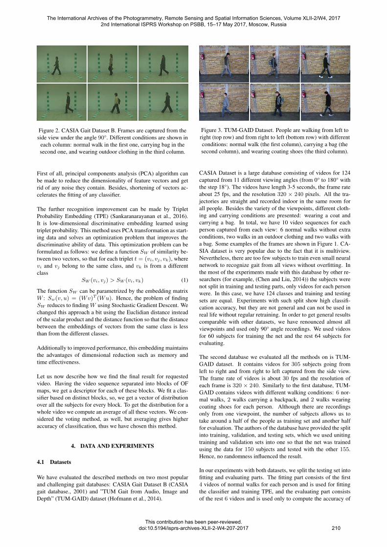
Figure 2. CASIA Gait Dataset B. Frames are captured from theside view under the angle 90°. Different conditions are shown in

each column: normal walk in the first one, carrying bag in thesecond one, and wearing outdoor clothing in the third column.

First of all, principal components analysis (PCA) algorithm canbe made to reduce the dimensionality of feature vectors and getrid of any noise they contain. Besides, shortening of vectors ac-celerates the fitting of any classifier.

The further recognition improvement can be made by TripletProbability Embedding (TPE) (Sankaranarayanan et al., 2016).It is low-dimensional discriminative embedding learned usingtriplet probability. This method uses PCA transformation as start-ing data and solves an optimization problem that improves thediscriminative ability of data. This optimization problem can beformulated as follows: we define a function SW of similarity be-tween two vectors, so that for each triplet t = (vi, vj , vk), wherevi and vj belong to the same class, and vk is from a differentclass

SW (vi, vj) > SW (vi, vk) (1)

The function SW can be parametrized by the embedding matrixW : Sw(v, u) = (Wv)T (Wu). Hence, the problem of findingSW reduces to finding W using Stochastic Gradient Descent. Wechanged this approach a bit using the Euclidian distance insteadof the scalar product and the distance function so that the distancebetween the embeddings of vectors from the same class is lessthan from the different classes.

Additionally to improved performance, this embedding maintainsthe advantages of dimensional reduction such as memory andtime effectiveness.

Let us now describe how we find the final result for requestedvideo. Having the video sequence separated into blocks of OFmaps, we get a descriptor for each of these blocks. We fit a clas-sifier based on distinct blocks, so, we get a vector of distributionover all the subjects for every block. To get the distribution for awhole video we compute an average of all these vectors. We con-sidered the voting method, as well, but averaging gives higheraccuracy of classification, thus we have chosen this method.

4. DATA AND EXPERIMENTS

4.1 Datasets

We have evaluated the described methods on two most popularand challenging gait databases: CASIA Gait Dataset B (CASIAgait database., 2001) and ”TUM Gait from Audio, Image andDepth” (TUM-GAID) dataset (Hofmann et al., 2014).

Figure 3. TUM-GAID Dataset. People are walking from left toright (top row) and from right to left (bottom row) with differentconditions: normal walk (the first column), carrying a bag (thesecond column), and wearing coating shoes (the third column).

CASIA Dataset is a large database consisting of videos for 124captured from 11 different viewing angles (from 0° to 180° withthe step 18°). The videos have length 3-5 seconds, the frame rateabout 25 fps, and the resolution 320 × 240 pixels. All the tra-jectories are straight and recorded indoor in the same room forall people. Besides the variety of the viewpoints, different cloth-ing and carrying conditions are presented: wearing a coat andcarrying a bag. In total, we have 10 video sequences for eachperson captured from each view: 6 normal walks without extraconditions, two walks in an outdoor clothing and two walks witha bag. Some examples of the frames are shown in Figure 1. CA-SIA dataset is very popular due to the fact that it is multiview.Nevertheless, there are too few subjects to train even small neuralnetwork to recognize gait from all views without overfitting. Inthe most of the experiments made with this database by other re-searchers (for example, (Chen and Liu, 2014)) the subjects werenot split in training and testing parts, only videos for each personwere. In this case, we have 124 classes and training and testingsets are equal. Experiments with such split show high classifi-cation accuracy, but they are not general and can not be used inreal life without regular retraining. In order to get general resultscomparable with other datasets, we have renounced almost allviewpoints and used only 90° angle recordings. We used videosfor 60 subjects for training the net and the rest 64 subjects forevaluating.

The second database we evaluated all the methods on is TUM-GAID dataset. It contains videos for 305 subjects going fromleft to right and from right to left captured from the side view.The frame rate of videos is about 30 fps and the resolution ofeach frame is 320 × 240. Similarly to the first database, TUM-GAID contains videos with different walking conditions: 6 nor-mal walks, 2 walks carrying a backpack, and 2 walks wearingcoating shoes for each person. Although there are recordingsonly from one viewpoint, the number of subjects allows us totake around a half of the people as training set and another halffor evaluation. The authors of the database have provided the splitinto training, validation, and testing sets, which we used unitingtraining and validation sets into one so that the net was trainedusing the data for 150 subjects and tested with the other 155.Hence, no randomness influenced the result.

In our experiments with both datasets, we split the testing set intofitting and evaluating parts. The fitting part consists of the first4 videos of normal walks for each person and is used for fittingthe classifier and training TPE, and the evaluating part consistsof the rest 6 videos and is used only to compute the accuracy of


This contribution has been peer-reviewed. doi:10.5194/isprs-archives-XLII-2-W4-207-2017

210

classification. It is worth noting that although the NN classifieris fitted using only fitting videos of testing subjects, the TPE istrained much quicker and better if we train it by both trainingand fitting sequences (all the information that is supposed to beknown in the algorithm).

4.2 Performance evaluation

All the algorithms have a classifier on their top that returns thevector of the distribution of the requested video sequence over alltesting subjects. We use Rank-k metrics equaled the ratio of sam-ples for which the correct label belongs to the set of k most prob-able answers to evaluate the results. Rank-1 metric is accuracy,that defines the ratio of the correctly classified videos. Besidesthe accuracy, we measure Rank-5 metrics.

4.3 Experiments and results

We evaluated all the methods described above on two considereddatasets. All the experiments can be divided into three parts.

1. Distinct learning and evaluating on each of the datasets;

2. Learning on one dataset and evaluating on both of them;

3. Joint learning on two datasets and evaluating on both ofthem.

These experiments aim to estimate the influence of differentmethods on the quality of classification and to learn how generalall these methods are. Ideally, the algorithm should not dependon the background conditions, the illumination, or anything otherthan the walking style of a person. So, it is worth evaluating howthe algorithm learned on one dataset works on the other one.

The first set of the experiments is made to evaluate the proposedapproach. We trained a net from scratch with the top layer of sizeequal the number of training subject. Then we trained a classifieron the learned descriptors using training and fitting data. Theresults of the experiments are shown in Table 3.

Method EvaluationArchitecture and Metrics Rank1 Rank5CNN (PCA 1100), L1 93,22 98,06CNN (PCA 1100), L2 92,79 98,06CNN (PCA 600), L1 93,54 98,38CNN+TPE (PCA 450), L2 94,51 98,70fusion CNN (PCA 160), L1 93,97 98,06fusion CNN (PCA 160), L2 94,40 98,06fusion CNN +TPE (PCA 160), L1 94,07 98,27fusion CNN +TPE (PCA 160), L2 95,04 98,06VGG (PCA 1024), L1 97,20 99,78VGG (PCA 1024), L2 96,34 99,67VGG+TPE (PCA 800), L1 97,52 99,89VGG+TPE (PCA 800), L2 96,55 99,78(Castro et al., 2016) CNN+SVM, L2 98,00 99,60

Table 3. Results on TUM-GAID dataset

Although the accuracy of our method does not exceed Castro’sRank-1, the second metrics is higher in our method. So, the cor-rect label is more often among the most probable ones.

The experiments show that training TPE having fewer dimen-sions always increases the accuracy as compared to common NN

classifier with L2 metrics. Nevertheless, L1 metrics often turnsout to be more successful. Despite the fact that TPE was trainedas optimization of Euclidean similarity, the best result is achievedon the NN classifier based on L1 distance between the embed-dings of the descriptors. Let us show the Table 4, where it iswritten in details what quality we get with different conditions.

Normal Backpack Shoes AvgMethod R1 R5 R1 R5 R1 R5 R1 R5VGG-like, L1 99,7 100 96,5 99,7 96,5 100 97,5 99,8CNN+SVM, L2

(Castro et al.,2016)

99,7 100 97,1 99,4 97,1 99,4 98,0 99,6

Table 4. Results for different conditions on TUM-GAID dataset

Knowing that VGG-like architecture gives the best result, weevaluated it on CASIA dataset. The accuracy on this datasetturned out to be much lower: 71, 80% of correct answers usingL2 distance and a bit more – 74, 93% when L1 is used.

Having the nets trained on each of the datasets we made the sec-ond set of the experiments investigating the generality of the algo-rithm – the experiments on transfer learning. TUM-GAID videosand the side view of CASIA look similar, so, we checked if onealgorithm can be used for both datasets. Despite good results ofthe algorithms on TUM-GAID dataset, it turns out that the accu-racy of the same algorithm with the same parameters on CASIAdataset is very low. The same happens on the other side when thenet trained on CASIA is used for extracting features for videosfrom TUM. These experiments were made using the best of con-sidered architectures – cropped VGG and the NN classifier basedon L1 metric without any extra embedding. Table 5 shows theaccuracy of such transfer classification.

Training SetTesting Set

CASIA TUM

CASIA 74,93 67,41TUM 58,20 97,20

Table 5. Results of transfer learning

All the results on CASIA are lower than on TUM-GAID andtransfer of the network weights noticeably worsens the initialquality.

The third part of experiments aims to investigate if the union ofall available data improves the recognition. All subjects in twodatabases are distinct, so, we can unite them to one dataset andtrain the net on this union. The evaluation of the algorithm wasmade individually for each dataset.

Result on TUM Result on CASIAMethod Rank1 Rank5 Rank1 Rank5VGG + NN, L1 96,45 99,24 72,06 84,07balancing learningVGG + NN, L2 96,02 99,35 70,75 83,02balancing learning

Table 6. Results of join learning

Because of the difference in sizes of two datasets we use, we hadto balance the input batches while training the net. Combining thebatch of OF blocks we use the same number of blocks from bothdatasets, so, the net sees samples from the small dataset morefrequently than from the large one. Despite such joint learning,the quality of the algorithm is lower than the quality of distinct



algorithms for each dataset. It means the overfitting in latter onesand the presence of dropout and regularization does not preventit.

5. IMPLEMENTATION DETAILS

We prepare the data using OpenCV library. The silhouette masksand bounding boxes were found by background subtraction,and the maps of optical flow were computed using Farneback(Farneback, 2003) method implemented in OpenCV. For CNNtraining Lasagne and Theano libraries were used. All the exper-iments were performed on a computer with 12 cores, 32 GB ofRAM and a GPU Nvidia GTX 1070. The most successful of con-sidered architectures, the VGG-like one, was trained from scratchon TUM-GAID dataset in about 16 hours. When the net is trainedit takes approximately 0.43 seconds to calculate all block descrip-tors for one four-second video and to classify it (including 0.14seconds of preprocessing).

6. CONCLUSIONS AND FURTHER WORK

The experiments show that available datasets are too small andnot enough for training general stable algorithm even for one cer-tain viewpoint. Having 155 subjects in the testing set and 6 test-ing videos for each of them we get only 930 testing samples (andeven fewer for a smaller database). It means that one correct an-swer changes the accuracy by about 0.1%, so the few percentdifference may be not significant.

Therefore the most important step for further improvements is tocollect new large gait dataset in order to have enough data fortraining complex deep models. Having appropriate database it isworth considering new CNN architectures and training methods.

REFERENCES

CASIA gait database., 2001. Online available:http://www.cbsr.ia.ac.cn/english/Gait%20Databases.asp.

Castro, F., Marin-Jimenez, M. and Guil, N.and Perez dela Blanca, N., 2016. Automatic learning of gait signatures forpeople identification. http://arxiv.org/abs/1603.01006.

Chatfield, K., Simonyan, K., Vedaldi, A. and Zisserman, A.,2014. Return of the devil in the details: Delving deep into con-volutional nets. In: Proc. BMVC.

Chen, J. and Liu, J., 2014. Average gait differential image basedhuman recognition. Scientific World Journal.

Chen, T., Goodfellow, I. and Shlens, J., 2016. Net2net: Acceler-ating learning via knowledge transfer. in international conferenceon learning representation. In: ICLR.

Farneback, G., 2003. Two-frame motion estimation based onpolynomial expansion. In: Proc. of Scandinavian Conf. on Im-age Analysis, Vol. 2749, p. 363370.

Feichtenhofer, C., Pinz, A. and Zisserman, A., 2016. Convolu-tional two-stream network fusion for video action recognition. In:CVPR.

Han, J. and Bhanu, B., 2006. Individual recognition using gaitenergy image. In: IEEE PAMI, Vol. 28(2), p. 316322.

Hofmann, M., Geiger, J., Bachmann, S., Schuller, B. and Rigoll,G., 2014. The tum gait from audio, image and depth (gaid)database: Multimodal recognition of subjects and traits. J. ofVisual Com. and Image Repres. 25(1), pp. 195 – 206.

Ioffe, S. and Szegedy, C., 2015. Batch normalization: Acceler-ating deep network training by reducing internal covariate shift.In: ICML.

Karpathy, A., Toderici, G., Shetty, S., Leung, T., Sukthankar, R.and Fei-Fei, L., 2014. Large-scale video classification with con-volutional neural networks. In: CVPR.

Liu, Y., Zhang, J., Wang, C. and Wang, L., 2012. Multiple hogtemplates for gait recognition. In: Proc. ICPR, pp. 2930–2933.

Ng, J., Hausknecht, M., Vijayanarasimhan, S., Vinyals, O.,Monga, R. and Toderici, G., 2015. Beyond short snippets: Deepnetworks for video classification. In: CVPR.

Sankaranarayanan, S., Alavi, A., Castillo, C. and R., C., 2016.Triplet probabilistic embedding for face verification and cluster-ing. arXiv preprint arXiv:1604.05417.

Simonyan, K. and Zisserman, A., 2014. Two-stream convo-lutional networks for action recognition in videos. In: NIPS,p. 568576.

Simonyan, K. and Zisserman, A., 2015. Very deep convolutionalnetworks for large-scale image recognition. In: ICLR.

Wang, L., Qiao, Y. and Tang, X., 2015. Action recognitionwith trajectory-pooled deep-convolutional descriptors. In: CVPR,p. 43054314.

Yang, K., Dou, Y., Lv, S., Zhang, F. and Lv, Q., 2016.Relative distance features for gait recognition with Kinect.https://arxiv.org/abs/1605.05415.

Zheng, S., Zhang, J., Huang, K., He, R. and Tan, T., 2011. Robustview transformation model for gait recognition. In: Proc. IEEEInternational Conference on Image Processing (ICIP), pp. 2073–2076.



gait recognition based on convolutional ... recognition based on convolutional neural networks a....

Documents