Improved Estimates of Correlation Coefficients

And Their Impact on the Optimum Portfolios

by

Edwin J. Elton*

Martin J. Gruber*

Jonathan Spitzer**

* Nomura Professor of Finance, Stern School of Business, New York University

** Doctoral Student, Stern School of Business, New York University

Abstract

To implement mean variance analysis one needs a technique for forecasting correlation

coefficients. In this article we investigate the ability of several techniques to forecast correlation

coefficients between securities. We find that separately forecasting the average level of pair-

wise correlations and individual pair-wise differences from the average improves forecasting

accuracy. Furthermore, forming homogenous groups of firms on the basis of industry

membership or firm attributes (eg. Size) improves forecast accuracy.

Accuracy is evaluated in two ways: First, in terms of the error in estimating future

correlation coefficients. Second, in the characteristics of portfolios formed on the basis of each

forecasting technique. The ranking of forecasting techniques is robust across both methods of

evaluation and the better techniques outperform prior suggestions in the literature of financial

economics.

2

Mean variance portfolio theory has had a major impact on both the theory of financial

economics and the practice of the financial community. Any use of portfolio theory requires

estimates of expected returns, variance of returns, and correlation coefficients. One way to

forecast future values is to use past values. However, even weak form efficiency would suggest

that past returns cannot be used to forecast future mean returns. On the other hand, no

interpretation of market efficiency implies that past values cannot be used to forecast future

variances and correlation coefficients. A second way to obtain estimates of future values is to ask

experts (security analysts). Many practitioners behave as if (and believe that) they can forecast

returns and variances. However, the large number of correlation estimates needed for even a

reasonable-sized portfolio optimization problem, combined with the nature of the estimates

(particularly the inability of an analyst, following a set number of stocks, to estimate the effect of

movements of other stocks on stocks he follows) makes the use of a model to estimate

correlation coefficients imperative. This leaves us with the problem of how best to use past data

to estimate future correlation coefficients.

The first attempts to forecast correlation coefficients are contained in Elton and Gruber

(1973) and Elton, Gruber and Ulrich (1978). They found that a forecast of all correlation

coefficients equal to the mean (the constant correlation model) performed as well or better than

other widely accepted forecasting technologies. Recently there have been a series of articles that

have revisited this issue. The remarkable result is that as discussed in the next section, despite all

the advances in modeling, the assumption that all correlations are identical to each other still

performs about as well as any other forecasting technique.

The purpose of this article is to develop and test techniques which outperform this simple

prescription. We do this by breaking the forecast of any pair-wise correlation in a particular

3

period into two parts: a forecast of the average correlation coefficient for the period in question

and a forecast of the difference of any pair-wise correlation from the forecasted average for the

period.

The paper is divided into five sections. In the first section we present a brief review of the

literature. In the second section we discuss the alternative forecasting techniques we will

examine. In the third section we discuss procedures for evaluating forecasts. In the fourth

section we present our results. The last section is the conclusion.

I. Literature Review

The earliest works on forecasting correlation coefficients are Elton and Gruber (1973)

and Elton, Gruber and Ulrich (1978). The authors showed that assuming all pair-wise correlation

coefficients were equal to the mean correlation coefficient (the constant correlation model)

produced better forecasts than those produced from assuming either a single index model or

multi-index models and considerably better than using pair-wise historical correlation (full

historical model).

Recently, a number of articles appeared that revisited this issue. These include Chan,

Korceski and Lakonishok (1999), Engle and Sheppard (2003), Jagnanathan and Ma (2003), and

Ledoit and Wolf (2003 and 2004). Chan, Korceski and Lakonishok (1999) examine forecasts of

both correlation coefficients and covariances. We will restrict our discussion to their forecasts of

correlation coefficients. The authors compared the forecasts produced by a full historical model,

a constant correlation model, and factor models ranging from one to ten factors. Their conclusion

was that constant correlation model had the lowest mean squared errors. They also compared

forecasts of correlation coefficients by examining the ability of alternative forecasting techniques

combined with one particular forecast of variances to produce the global minimum variance

4

portfolio with the smallest variance, and found the same ordering of techniques. Thus, despite

using all the improvements in modeling that have been produced in the last 30 years, they find

that the constant correlation still works best.

Jagannathan and Ma (2003) also examine the ability of alternative estimates of the

correlation matrix to produce the minimum variance portfolio. They first point out that placing

upper and lower bounds on the amount invested in any security in the global minimum variance

portfolio produces the same solution obtained by shrinking many of the extreme covariance

estimates toward the mean. They compare the risk of the minimum variance portfolio when

imposing upper and lower bounds with the risk when covariance estimates are obtained from:

1. The single index model.

2. Ledoit’s (1999) shrinkage procedure.

3. Fama and French’s three-factor model.

4. Connor and Korajcyzk’s five-factor model.

They find all models produce about the same risk. Of all models, the Ledoit shrinkage

procedure works best, but not significantly so. Using weights of one-half on the estimates

produced by the single index model and one-half on the historical pair-wise estimate works as

well as Ledoit’s optimal shrinkage estimator. Jagannathan and Ma never consider the constant

correlation model.

Under the assumption of IID stock returns and a quadratic loss function, Ledoit (1999)

develops an optimal weighting on two estimates of the variance-covariance matrix – the

historical pair-wise value itself and the estimate produced by the Sharpe single index model.

Ledoit (1999) tests the ability of his weighted estimate of the variance covariance matrix to

produce a lower risk portfolio against competitive models when short sales are allowed. The two

5

portfolios he used to compare forecasts are the global minimum variance portfolio and a

portfolio which has minimum variance at an expected return of 20%. The return estimate for

each stock is its historic return over a ten-year period. Ledoit finds that the average of the Sharpe

and historical covariance matrix using his shrinkage estimator produces portfolios with lower

risk than a number of other estimators proposed in the literature.

In a later article (Ledoit and Wolf (2004)) the authors conclude that shrinking the

historical pair-wise correlation towards a model which assumes all correlations are the same (the

constant correlation model) produces even better results than shrinking towards the Sharpe single

index model.

Since Jagannathan and Ma found a fifty-fifty combination of the Sharpe single index and

historical pair-wise worked best, and since Ledoit and Wolf find it even better to use the constant

correlation, either the constant correlation by itself (Chan, Korceski & Lakonishok) or a

combination of the constant correlation and historical pair-wise values represent the models that

have been shown to perform best.

Engle and Colacito (2003) develop techniques for evaluating alternative forecasts of

variance covariance matrices. They suggest developing alternative estimates of the variance,

covariance matrix along with a random set of forecasted mean returns for each security. These

estimates are used to select a portfolio with a prespecified expected return and then the future

variance for this portfolio is computed. The same procedure is repeated many times. The superior

forecasting technique is the one that produces the lowest variance across alternative vectors of

expected returns. The loss from using the inferior technique is computed as the increment in

expected return necessary for the inferior technique to have the same Sharpe ratios.1

1 Differences in realized return are ignored, since ex ante all forecasting techniques have the same expected return for each security.

6

II. Forecasting Correlation Coefficients

In the previous section we discussed the literature on forecasting correlation coefficients.

In this section we outline our approach, and more specifically the models we will use to forecast

pair-wise correlations of stock returns. As discussed earlier, researchers have found that the

average of the prior periods’ pair-wise correlation coefficients (the constant correlation model)

forecasts future pair-wise correlation coefficients about as accurately as more complicated

techniques. In the first part of this section we will discuss techniques for improving the forecast

of the future average correlation. We will then examination whether we can improve on this

estimate by forecasting pair-wise deviations from the mean.2

A. Estimates of the Mean Correlation Coefficients

The simplest estimate of the mean correlation coefficient, and one used by all prior

researchers, is simply to set it equal to its prior period’s value. The question remains as to

whether more sophisticated approaches can lead to better estimates. In this paper we investigate

standard techniques of time series analysis to see if they improve forecasting.

Techniques for constructing a model of the stochastic process that has generated an

observed set of data and subsequently using the parameterized model to forecast future values of

the variable under study are well documented in the literature of econometrics.3 In this paper we

will fit the general class of ARIMA (Auto Regressive Integrated Moving-Average) techniques to

a long-time series of average correlation coefficients to see if they produce better forecasts than

simply using the prior period’s value. We will also examine an exponential smoothing model of

past values to see if this improves forecasts because Engle and Sheppard (2003) provide

2 The separation of the forecast into a mean forecast and deviations from the mean also deals with the issue raised by Elton and Gruber (1973), who found that many ways of forecasting pair-wise correlation coefficients produced biased estimates. In order to adjust for this bias, one needs forecasts of the mean correlation coefficient. 3 For an excellent discussion see Judge et al (1988)

7

evidence that this exponential model outperforms more sophisticated time series models in

estimating correlation coefficients.4 Finally, we will explore the use of a simple moving average

model to forecast the average future correlation.

B. Estimating Differences in Correlation Coefficient from the Mean

Early research indicated that subdividing firms into groups could lead to better estimates

of pair-wise correlation coefficients.5 In this model the correlation between any two firms in a

group is set equal to the average of all pair-wise correlations between firms in the group and the

correlation between any firm in one group and a firm in a second group is set equal to the

average of the correlations between any firm in the first group and any firm in the second group.

This leaves us with the problem of designing appropriate groups.

At one extreme is the assumption that only one group exists. This leads to the constant

correlation model which has been shown to lead to very good forecasts compared to other types

of models. At the other extreme is the assumption that each firm is its own group, which has

been shown to lead to very poor forecasts of the future (individual pair-wise correlations).

The issue remains as to how to form an intermediate set of groups so that group

membership conveys real information about correlation patterns. We will explore two metrics for

grouping: industry membership and firm characteristics.

For each grouping technique, forecasts are formed using weekly return data as follows.

Each year all NYSE common stocks in the top eighty percent by market capitalization with

enough price data to measure weekly returns in the following year were selected. Grouping was

4 It is possible that incorporating past values of other variables may improve on forecasts based solely on past values of the variable itself. We examined this for models incorporating a number of variables including interest rates, dividend yields and measure of the variance of the market portfolio. The contemporaneous variance of the market portfolio was very useful in explaining mean correlation. However, the predictive equation in conjunction with a forecaster of market variance did not perform better than the past mean of the correlation coefficient. 5 See Elton & Gruber (1973)

8

performed using data available for the five years prior to the forecast year. In each year we

prepared for each group a forecast of the average correlation within and between groups based

on the past five years. This was then used to forecast the correlation in the following year. This

was repeated for each forecast year from July 1968 to July 2001.

A standard metric for classifying firms used by the financial community is industry

membership. Industries are frequently formed by examining SIC codes. Ken French has formed

industry groupings based on combining four-digit SIC industry codes.6 He does this for different

sized aggregations based on the tradeoff between parsimony of industry groups and homogeneity

of industry groups. We examine forecast accuracy for French’s 10, 17 and 30 industry groups.

The alternate way to group firms is on firm characteristics. The literature of financial

economics suggests that there are a set of variables which affect returns. These include

influences suggested by Fama and French such as the beta with the market, measures of size and

measures of book-to-market. In addition, several studies have indicated that dividend yield might

play a role in determining prices.7

If variables are in the return-generating process, then the covariance between securities is

determined by the product of the sensitivities (betas) and the variance of the factor. For example,

for the single index model the covariance is 2im jmβ β σ . Multi-factor models have not performed

well in estimating correlations.8 However, grouping on firm characteristics may perform well

even when their direct use to estimate correlations did not, if there is information in the

sensitivities, but sensitivities have a large estimation error.

6 See http://mba.dartmouth.edu/pages/faculty/ken.french/ 7 See, for example, Campbell & Shiller (1988).

9

When examining firm characteristics as a grouping metric we used deciles parameterized

over the same five years discussed earlier. The characteristics we examined were beta on the

market and beta on Fama & French’s small-large size variable and high-low book-to-market

variable. We also investigate certain firm characteristics which have been suggested elsewhere in

the literature. These include variance, dividend yield, and total capitalization. We also used a

two-way classification on total capitalization and market beta. Finally, we will examine the

ability of combinations of the best forecasting techniques described above to produce estimates

of future correlation coefficients.

III. Evaluation

In this section we will discuss the techniques we will use for evaluation of each of our

forecasting models. To do this we first adjust the average forecasted pair-wise correlation from

each forecasting model so that it is equal to the best forecast of the average as determined in the

earlier section of this paper.

The most common use of correlation coefficients is as an input for the construction of

optimum portfolios. In what follows we will assume annual holding periods and that the manager

at the beginning of each year uses the latest estimates of each correlation coefficient. A manager

utilizing correlation coefficients should want to use the forecasting model that produces the more

accurate estimates. Accuracy is important so that a portfolio is selected that is close to true

optimum. Forecasting accuracy will be measured as root mean squared error:

/i j i jm m

8 We are forecasting correlations. The correlation between firm i and firm j if the single index model holds is σ σ σ σ

10

( )

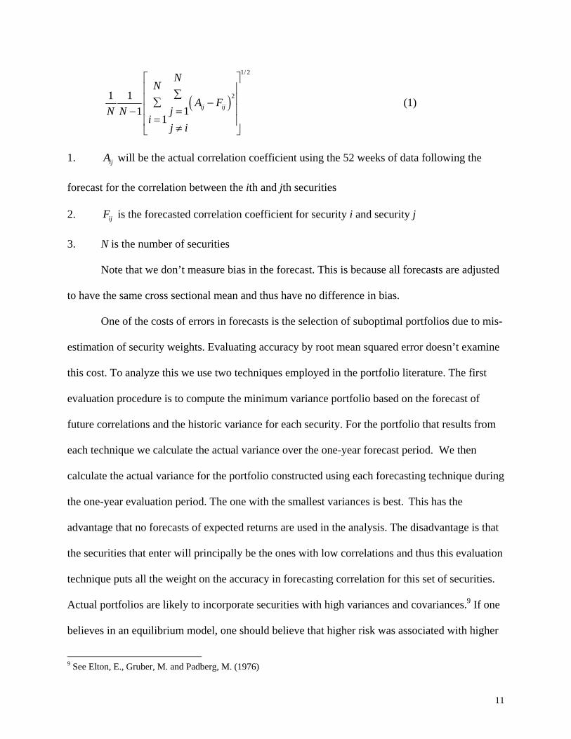
1/ 2

21 111

1ij ij

NN

A FjN N

ij i

⎡ ⎤⎢ ⎥∑⎢ ∑ −⎢ =−=⎢ ⎥≠⎣ ⎦

⎥⎥

(1)

1. ijA will be the actual correlation coefficient using the 52 weeks of data following the

forecast for the correlation between the ith and jth securities

2. is the forecasted correlation coefficient for security i and security j ijF

3. N is the number of securities

Note that we don’t measure bias in the forecast. This is because all forecasts are adjusted

to have the same cross sectional mean and thus have no difference in bias.

One of the costs of errors in forecasts is the selection of suboptimal portfolios due to mis-

estimation of security weights. Evaluating accuracy by root mean squared error doesn’t examine

this cost. To analyze this we use two techniques employed in the portfolio literature. The first

evaluation procedure is to compute the minimum variance portfolio based on the forecast of

future correlations and the historic variance for each security. For the portfolio that results from

each technique we calculate the actual variance over the one-year forecast period. We then

calculate the actual variance for the portfolio constructed using each forecasting technique during

the one-year evaluation period. The one with the smallest variances is best. This has the

advantage that no forecasts of expected returns are used in the analysis. The disadvantage is that

the securities that enter will principally be the ones with low correlations and thus this evaluation

technique puts all the weight on the accuracy in forecasting correlation for this set of securities.

Actual portfolios are likely to incorporate securities with high variances and covariances.9 If one

believes in an equilibrium model, one should believe that higher risk was associated with higher

9 See Elton, E., Gruber, M. and Padberg, M. (1976)

11

expected return. Thus, the evaluation of forecasts should span the whole range of securities, not

just securities with low correlations and variances. The alternative is to explore the accuracy of

portfolios over the full range of risks. This requires making expected return forecasts. To do this

we take the historical realized return and standard deviation of return for each security. For each

security we draw a random return (for a year) from the historical distribution for that security.

The random return drawn for each security will be used as an estimate of the expected return for

that security. These estimates, along with the historical variance and forecasted correlations, will

be used to select a portfolio with the minimum variance at the average return across all securities

in the sample period.10 The variance of this portfolio during the evaluation year will be compared

across different forecasting techniques. The estimation procedure for computing expected returns

on each security will be repeated a number of times.

IV. Results

In this section we will discuss the results for the forecasts of the overall mean and the

results for forecasting pair-wise correlations between individual firms.

A. Forecasts of Mean Correlation Coefficient

First we will examine the forecast accuracy of different estimates of the average pair-

wise correlation coefficient. Table 1 shows the root mean squared errors for various techniques

of forecasting the mean correlation coefficient computed for each one-year period over 33 years.

Column 1 measures the accuracy of the forecast of next year’s actual mean for various

techniques. More exactly, Column 1 presents the root mean squared error of the difference

between the actual mean and the forecasted mean. Column 2 measures the RMSE error when

applying these mean forecasts as forecasts of next year’s individual pair-wise correlations. The

10 This procedure is suggested in Engle and Sheppard (2004).

12

estimate of next period’s mean from the AR(1) model and using the mean that occurred in the

previous period perform poorest.11 In addition to these models we investigated a rolling average

of the last five years average correlations and an exponential smooth of the five averages with a

coefficient of .5.12 Not only did these techniques outperform the other techniques, but the rolling

average and the exponential smooth had lower root mean squared errors than using the actual

average mean over the full sample. This is especially interesting since the full sample overall

actual average uses data that is not available at the time of the forecast. There is no clear choice

between the five-year rolling average and the exponential smooth. In what follows we will

present results for the rolling average, but the results for the exponential smooth are very similar.

B. Forecasting Differences Based on Mean-Squared Error Tests

Tables 2, 3 and 4 compare root mean squared errors for the rolling average forecast of the

mean correlation coefficient combined with individual and group mean forecasts of deviations

from the mean correlation coefficient. The way in which this was done was to adjust each

forecast by the difference between the mean from any forecasting technique and the best forecast

of the mean as described in Section A. This results in each forecasting technique having the same

mean so that differences in forecasting ability are due entirely to forecasted differences from this

common mean. Table 2 shows the results for industry groupings compared to using individual

and constant correlation forecasts. Table 3 presents results when firms are grouped by one or

more of their characteristics, and Table 4 presents results for mixtures of techniques. Except

where noted, all forecasts are prepared by taking a five-year moving average of the correlation

estimated each year using the technique being examined.

11 We estimated a number of alternative time series models and ran a number of tests of correlation patterns. The only auto-regressive model with any empirical support was an AR(1) model, and its support was weak. 12 The .5 coefficient was pre-specified. However, when we examined other choices the .5 performed best.

13

First, examine Table 2. Forecasting techniques are listed in order from the one that

performed worst down to the one which performed best. Using the latest year’s individual pair-

wise deviations from the mean for individual correlations produced the poorest forecasts. The

large errors associated with using last period’s historical pair-wise correlations is consistent with

previous literature (see, for example, Jobson and Korkiel (1980), Jorion (1985), and Frost and

Savarino (1988). However, using an average of the last five individual pairwise correlations

(rolling individual pairwise correlations) produced forecasts better than the constant correlation

model and much better than last period’s pairwise correlation. Furthermore, the differences are

statistically significant at the .01 level. Averaging the pair-wise correlation over time makes a

substantial difference in forecasting ability.

Both logic and cursory examination of the raw data suggest that the correlation is higher

between firms if they are the same industry than if they are in different industries. The next

model we examined is labeled the within and between model. This model uses only two different

mean correlation coefficients, one if both firms are in the same industry (regardless of the

industry) and one if they are in different industries. The within and between model has lower

root mean square errors than does the overall mean and the rolling individual pair-wise

correlations, and the differences are significant at the .01 level. The question remains whether

results would be improved by using separately estimated mean pair-wise correlation coefficients

within each industry and between each pair of industries.

We investigate forecasting for three different number of industry groupings. Firms are

divided into 10, 17 and 30 groups where the groupings follow French’s categorization. Each of

these models uses a different average correlation within each industry and between each pair of

industries. For example, for a 10-industry model we have 10 10 10102

• −+ averages of

14

correlation coefficients. The root mean squared error improves as we partition four digit SIC

industry into more groups, and the improvement is significant at the .01 level in each case. Thus,

across all industry groupings the 30 industry grouping works best.

Table 3 shows the root mean squared errors when we group on firm characteristics rather

than French industry groupings as well as the errors using a constant correlation model. The firm

characteristics that are explored are betas on the Fama French factors (namely high minus low

beta and small minus large beta), variance, dividend yield, market beta and capitalization. When

we used grouping metrics that required past data to estimate sensitivities, we lose a small number

of firms from our sample because of additional data requirements. Thus the RMSE for the

constant correlation model is computed over a slightly different sample. The two grouping

metrics that had the best performance in terms of mean squared error were market beta and size.

When we group on these two characteristics together (five divisions on beta and five on size) we

get the lowest root mean square error.13 Note that all differences in root mean errors in adjacent

techniques are statistically significant except for the comparison between dividend yield and

market beta.

A number of authors have suggested combining historical pairwise correlations with

forecasts from another model. Jagannathan and Ma (2003) find that a combination of the single

index model and historical pairwise correlation coefficient work best. Ledroit and Wolf (2003)

find that combining the constant correlation model and the historical pair-wise correlation

coefficient works better than combining the single index model and the historical pair-wise

13 A necessary condition for a grouping technique to lead to improved forecasting is that there is substantial variation in the forecasted correlation coefficients from cells within the group compared to just using the overall mean. Except for capitalization and CAPM beta there is little variation in forecasted correlations across cells and only in these cases does the pattern make economic sense.

15

correlation coefficient. Thus the combination of the constant correlation forecast and historical

pair-wise correlation coefficient is the target to beat.

Table 4 shows the mean square error for equal weighting of each of the techniques with

the forecast from a rolling average of individual pair-wise correlations. Once again there are

slight differences in the sample so that the RMSE for the mean overall correlation is slightly

different from its value in prior tables. Similar to others, we find that an average of overall mean

and individual estimates performs better than the overall mean by itself. Given the results in the

prior section, it is not surprising that replacing the overall mean with the 30 industry mean or the

grouping using size and beta improves the mean squared forecast error. The last row involves

combining the forecasts from the 30 industry grouping and the characteristic grouping along with

historical forecasts.14 This provides the best results. Once again, all differences in adjacent

techniques are significant at the 1% level.

Although most of the differences are statistically significant, it is worthwhile examining

whether there are sufficient differences between them to impact decisions. . In a later section we

will examine more sophisticated tests of improvement in Sharpe ratios due to improved

forecasting. Before doing so, however, we can get an idea of whether or not the lower mean

squared error is meaningful by performing the following exercise. Assume the only technique

that could be used to forecast correlations is the constant correlation model. Compute the mean

square error for a forecast equal to the true mean in every period. Now introduce an error in the

mean forecast. How big would the error have to be to produce the same change in root mean

squared error as we observe between two different forecasting models shown in Tables 2, 3 or 4.

To compute this we proceed as follows:

16

The average mean square error (AMSE) for two forecasting techniques can be defined as

21

1 1(1) ( )1 ij ijAMSE A F

N N=

− ∑∑ − (2)

22

1 1(2) ( )1 ij ijAMSE A F

N N=

− ∑∑ − (3)

Where ijA and are the actual and forecast respectively, and the subscript before the F indicates the forecasting technique used.

ijF

The techniques are ordered so that AMSE(2) > AMSE(1). The mean square error using the true mean (TM) as a forecast at period T+1 is

21 1( ) ( )1

AMSE TM Aij AN N

=− ∑∑ − (4)

Now define e as an error in estimating the mean such that if A e+ were used to estimate the correlations for all forecasts, e would result in the AMSE(e) – AMSE(TM) being equal to AMSE(2) – AMSE (1).

( ) 21 1( )1 ijAMSE e A A e

N N⎡ ⎤= − +⎣ ⎦− ∑∑ (5)

since ( )1 1 ( )1 ijA A e O

N N− =

− ∑∑

Then

( ) 21 1( )1 iiAMSE e A A e

N N= − +

− ∑ ∑

thus (6) 2 (2) (1)e AMSE AMSE= −

This formula allows us to determine how large an error in the forecast of the average

correlation efficient would produce the difference in forecast error actually observed between

14 We also tried unequal weighting where the weights were obtained from a regression of forecasted correlations (using data from six months to one year prior to obtain the forecasts) on the prior year’s actual. There was no discernible difference, probably because the regression weights were close to equal.

17

any two forecasting techniques. By using equation (6) and the data in Table 2 we see that the

RMSE, from using the 30 industry grouping rather than the constant correlation model, is

equivalent to mis-estimating the mean

( ) ( )1/ 22 2.1698 .1672 .0296e ⎡ ⎤= − =⎣ ⎦

or a percentage error in the average correlation of 17.4%. Thus the small difference in mean

square error between the constant correlation model and the thirty industry model is equivalent to

a sizable percentage change in mis-estimating the average correlation between stocks.

We can also compute the error in the mean that is equivalent to the difference in error

from using the best of our fundamental models (Table 3) versus the constant correlation model.

The error in the mean that produces an equivalent difference in RMSE is .0385 or 22.6%.

Finally, employing the best forecasting technique which is weighted average of the

rolling individual pair-wise correlation coefficients, the 30 industry forecasts and the forecast

based on an equal weighting of market beta and size, the error that produces RMSE equivalent to

the difference in RMSE of the best technique and a combination of constant correlation mean

plus historical pair-wise correlation coefficient is .0494 or 27.11% of the average mean

correlation coefficient.

C. Forecasting Differences from the Mean-Estimating Efficient Frontiers

The second method we use for evaluating forecasting techniques is to examine how

well they do in producing low variance portfolios in the future. In each year we selected 100

securities at random. Using the prior five years’ weekly returns we estimated the mean return

and variance for each security. As the expected return for any security we use a draw from

the expected return distribution for that security. To obtain this distribution we used the

historical mean return and the historical standard deviation divided by the square root of N

18

and assumed a normal distribution. For variance we use the historical variance for each

security. The pair-wise correlation coefficient is estimated separately as the correlation

forecast for each of the models which performed best in Tables 2, 3 and 4. For each

forecasting technique we solved for portfolio weights for the minimum variance portfolio and

for the portfolio with a mean return equal to the average mean return across the 100 security

sample. In each year we repeated the process 100 times. Since the mean return is the same

for all correlation forecasting techniques, the characteristic of the portfolios that can be used

for evaluation is variance. The most accurate correlation forecast is the technique that has the

lowest variance in the year following portfolio formation. Table 5 shows the results. The

results for the minimum variance portfolios are shown in Column 2 and for mean return are

shown in Column 3. The results reinforce what we observed when we examined squared

error. The combination of the industry grouping size and beta grouping and rolling pair-wise

correlation had the lowest ex-post variance both for the minimum variance portfolio and for

the optimum portfolio at the mean return on the sample. Next best was the characteristic

grouping, next industry grouping, and finally constant correlation. All of the differences

between adjacent techniques are statistically significant at the one percent level. In addition,

when we divide the sample in half, each sub-sample has the same rankings and all

differences between adjacent techniques are statistically significant.

Another way of judging significant is to look at the increase in return between

forecasting techniques that would have to occur to produce the same Sharpe radio. To have

the same Sharpe ratio combining individual forecasts with the overall mean rather than the

combination of three forecasts would require an extra 38 BP return per year. While this is a

small difference, using the superior technique is no more costly, so it is worth doing.

19

Conclusion

In this paper we examined the ability of several techniques to forecast correlation

coefficients between securities. Techniques are evaluated both in terms of forecast accuracy

and their impact on the characteristics of optimum portfolios.

One distinguishing feature of this research is that we forecast the average level of

correlations separately from pair-wise differences from the overall average. This two-step

approach improves the forecast of correlations.

In exploring differences in pair-wise correlations from the average level of correlations

we examine several alternative methods for forming groups and forecasting correlations

within and between groups. Past researchers have explored the two extreme methods of

grouping: each firm is a group and all firms are in one group. We find that grouping firms by

either industry or several of the firm characteristics that have been shown to be part of the

return generating process improves forecasts compared to most suggestions contained in the

literature. Finally, preparing forecasts based on a simple weighted average of three forecasts

namely those obtained by grouping into 30 industries and grouping by Size and Beta and

historical pair-wise correlations, provides forecasts that out performs all forecasting

techniques suggested in the literature.

This out performance is robust whether performance is measured by

1.) Minimum squared forecast error

2.) Minimum future variance of portfolios selected. This is true whether portfolios with

returns equal to historic levels are examined or global minimum variance portfolios

are examined.

20

The differences in the portfolios selected by alternative forecasting techniques translate into

differences in Sharpe ratios which are economically meaningful.

21

Root Mean Squared Errors For Forecasts of the Overall Mean

Table 1

MEAN INDIVIDUAL Previous Year .0732 .1721 AR(1) .1196 .1856 Rolling Average .0656 .1698 Smoothed .0658 .1698 Full Sample Mean .0673

This table presents root mean square errors from different techniques for forecasting the average pairwise correlation between stocks in each year from 1968 to 2001. The column labeled “Mean” contains the RMSE in forecasting the average correlation, while the column labeled “Individual” shows the average RMSE when the forecasted mean is used as an estimate for all pairwise correlations. The row labeled “Previous Year” forecasts the next year’s average correlation coefficient as equal to the latest observed one-year average. AR(1) model is estimated over the entire sample period and then forecasts are prepared from the past five years using the estimated AR(1) process. “Rolling average” is a simple moving average of the five previous years average correlation. “Smoothed” is an exponential smooth of the past five years average with an exponential weight of .5. “Full Period Mean” is the average over the entire sample period of each year’s average correlation coefficients.

22

Root Mean Squared Errors Using Industry Groupings

Table 2

Statistical Significance

RMSE

Difference From Constant Correlation

Difference from Technique Shown in Previous Row

Individual Pairwise Correlations .2056 .01 Constant Correlation .1698 .01 Rolling Individual Pairwise Correlations .1694 .01 .01 Within and Between (10 industries) .1692 .01 .01 10 Industry .1678 .01 .01 17 Industry .1675 .01 .01 30 Industry .1672 .01 .01 This table contains the average yearly RMSE and statistical significance for pairwise correlation coefficients produced by the forecasting methods shown in the table. The column labeled RMSE is the average root mean square error for the techniques named in each row. The table indicates whether the differences are significant at better than the 1%, 5% or 10% level. The row labeled “Individual Pairwise Correlations” forecasts next year’s pairwise correlation as equal to the prior year’s pairwise correlation. “Rolling Individual” uses the average of the previous five years. “Constant Correlation” forecasts each pairwise correlation as equal to the average of the past five years’ average correlation coefficients. The other entries involve partitioning firms into groups and using a five-year average of the correlations within and between groups to forecast the pairwise correlation for the future. “Within and Between” splits the firms into 10 industries but assumes only two correlation numbers are necessary: one for the firms in the same industry, and one for any firms in different industries. The rows labeled 10, 17 and 30 divide firms into that number of industries. The forecasting model assumes that the forecast for any two firms is equal to the five-year average of the average correlation for firms in an industry if they are in the same industry or a five-year average of the average correlation between industries represented by these two firms if they are in different industries.

23

Root Mean Square Errors For Characteristic Grouping

Table 3

STATISTICAL SIGNIFICANCE

Difference from Constant Correlation

Difference from Technique Shown in Previous Row

Constant Correlation .1705 Beta on high-low .1702 .01 .01 Beta on small-big .1700 .01 .01 Variance .1694 .01 .01 Dividend Yield .1691 .01 .01 Market Beta .1689 .01 --- Size .1680 .01 .01 Size Plus Market Beta .1661 .01 .01

This table presents the RMSE from forecasting future pairwise correlation coefficients, where groups are formed by ranking on the criteria shown in the first column and then putting firms into deciles based on that rank (twenty-five groups in the case of the last row). Constant correlation, as in the previous table, forecasts each pairwise correlation as equal to the five-year average of the average pairwise correlation coefficients in each year. For the other criteria, ranking is performed on

1. Beta on the Fama-French book-to-market factor. 2. Beta on the Fama-French small-large factor. 3. Variance of return . 4. Dividend yield from the previous year. 5. Beta with the S&P Index. 6. Capitalization which is the total market value of the companies’ stock. 7. Capitalization plus market beta is a dual sort on five capitalization groups and

five market betas. Five years of monthly data are used to form groups and so the sample requirements are stricter than those in Table 2. Because of this, the numbers for the Constant Correlation row differ from the number in Table 2.

24

Root Mean Square Error for Combined Groups

Table 4

Statistical Significance

Full Sample

Difference from Constant Correlation

Difference from Technique Shown in Previous Row

Constant Correlation* .1650 .01 Thirty Industry .1646 .01 .01 Size and Beta .1639 .01 .01 Thirty Industry Plus Size and Market Beta Regression

.1632 .01 .01

The forecasts in this table are equal to an average of the forecast shown in the left-hand column and the five-year rolling average of individual pairwise correlations. Each of the forecasts in the left-hand column breaks firms into groups based on the criteria listed. Pairwise correlation between these groups is estimated as the five-year average of the average correlation between all firms in the group the two firms represent if they are in the same group or the five-year average of the average correlation between firms in the two groups they are members of ,if the firms are in different groups, thirty industry forms 30 groups based on the French categorization of industries. Size and beta used a two-way sort of firms into 25 groups based on market value of equity and the beta with the market estimated over five years. For 30 industry and market beta, weights of 1/3 are used for each of these estimates and the historic pairwise correlation. * The constant correlation not combined with individual forecasts has a root mean square error of .1705. All other techniques in the table produce smaller RMSE and the differences are each significant at the .01 level.

25

Realized Variance

(weekly in percent)

Table 5

GMV Target Constant Correlation .139 .154 30 Industry Mean .133 .151 Size and Beta .129 .150 Combination .125 .149

Each year the forecasted correlations are used along with the prior variance and a draw from the distribution of the mean return. The variance shown is the actual variance in the subsequent year. For Target, an optimum portfolio is constructed at the mean historical return. The realized variance shown is over all years and 100 random samples per year. All variances are significantly different from the prior at higher than the 1% significance level.

26

References

Best, Michael J. and Robert R. Grauer, 1991, On the Sensitivity of Mean-Variance-Efficient

Portfolios to Changes in Asset Means: Some Analytical and Computational Results,

Review of Financial Studies 4, 315-42.

Black, Fisher and Robert Litterman, 1992, Global Portfolio Optimization, Financial Analysts

Journal, September-October, 28-43.

Campbell, John and Robert Shiller, 1998, The Divident Price Ratio and Expectation of Future

Dividends and Discount Factors. Review of Financial Studies 1, 195-228.

Chan, Louis K.C., Jason Karceski and Josef Lakonishok, 1999, On Portfolio Optimization:

Forecasting Covariances and Choosing the Risk Model, Review of Financial Studies 12,

263-78.

Elton, E.J. and M.J. Gruber, 1973, Estimating the Dependence Structure of Share Prices –

Implications for Portfolio Selection, Journal of Finance 28, 1203-1232.

Elton, E.J., Martin J. Gruber and Manfred Padberg (1976), Simple Criteria for Optimal Portfolio

Selection, Journal of Finance 31(5), 1341-1357.

Elton, E.J., M.J. Gruber and T. Ulrich, 1978, Are Betas Best? Journal of Finance 23,

1375-1384.

Engle, Robert and Kevin Sheppard, Theoretical and Empirical Properties of Dynamic

Correlation Multivariate [garch]. Working paper, New York University.

Frost, Peter A. and James E. Savarino, 1986, An Empirical Bayes Approach to Efficient

Portfolio Selection, Journal of Financial and Quantitative Analysis 21, 293-305.

Frost, Peter A. and James E. Savarino, 1988, For Better Performance: Constrain Portfolio

Weights, Journal of Portfolio Management 15, No. 1, 29-34.

27

Jagannathan, Ravi and Tongshu Ma, Risk Reduction in Large Portfolios: A Role for Portfolio

Weight Constraints, Forthcoming, Journal of Finance, 2003.

Jobson, J.D. and B. Korkie, 1980, Estimation for Markowitz Efficient Portfolios, Journal of

the American Statistical Association 75, 544-54.

Jobson, J.D. and B. Korkie, 1981, Putting Markowitz Theory to Work, Journal of Portfolio

Management, Summer, 70-74.

Jorion, Philippe, 1985, International Portfolio Diversification with Estimation Risk, Journal of

Business 58, 3, 259-278.

Jorion, Philippe, 1986, Bayes-Stein Estimation for Portfolio Analysis, Journal of Financial

and Quantitative Analysis, 21, 3, 279-292.

Ledoit, Olivier and Michael Wolf, 2003, Improved Estimation of the Covariance Matrix of Stock

Returns with an Application to Portfolio Selection, Journal of Empirical Finance 10, 5,

December 2003.

Ledoit, Olivier and Michael Wolf, 2004, Honey, I Shrunk the Sample Covariance Matrix,

Journal of Portfolio Management, 31, 1.

28