implications of current spatial management measures for
TRANSCRIPT

Implications of current spatial management measures for AFMA ERAs for habitats
Roland Pitcher, Nick Ellis, Franziska Althaus, Alan Williams, Ian McLeod,
Rodrigo Bustamante, Robert Kenyon, Michael Fuller
June 2016
FRDC Project No 2014/204
OCEANS & ATMOSPHERE FLAGSHIP

ii | Implications of current spatial management measures for AFMA ERAs for habitats
© 2016 Fisheries Research and Development Corporation. All rights reserved.
National Library of Australia Cataloguing-in-Publication entry:
Pitcher, C. R. (Clifford Roland) Implications of current spatial management measures for AFMA ERAs for habitats / FRDC project; no. 2014/204 C. Roland Pitcher, Nick Ellis, Franziska Althaus, Alan Williams, Ian M. McLeod, Rodrigo H. Bustamante, Robert A. Kenyon, Michael E. Fuller.
Includes bibliographical references. ISBN: 978-1-4863-0685-5 (ebook : pdf)
Ocean bottom ecology--Australia. Ecological risk assessment--Australia. Fisheries--Environmental aspects--Australia. Trawls and trawling--Australia. Aquatic habitats--Australia.
CSIRO Oceans and Atmosphere
577.770994
2016
Ownership of Intellectual property rights Unless otherwise noted, copyright (and any other intellectual property rights, if any) in this publication is owned by the Fisheries Research and Development Corporation and CSIRO Oceans & Atmosphere.
This publication (and any information sourced from it) should be attributed to:
Pitcher, C.R., Ellis, N., Althaus, F., Williams, A., McLeod, I., Bustamante, R., Kenyon, R., Fuller, M. (2016) Implications of current spatial management measures for AFMA ERAs for habitats — FRDC Project No 2014/204. CSIRO Oceans & Atmosphere, Published Brisbane, November 2015, 50 pages.
Creative Commons licence All material in this publication is licensed under a Creative Commons Attribution 3.0 Australia Licence, save for content supplied by third parties, logos and the Commonwealth Coat of Arms.
Creative Commons Attribution 3.0 Australia Licence is a standard form licence agreement that allows you to copy, distribute, transmit and adapt this publication provided you attribute the work. A summary of the licence terms is available from creativecommons.org/licenses/by/3.0/au/deed.en The full licence terms are available from creativecommons.org/licenses/by/3.0/au/legalcode
Inquiries regarding the licence and any use of this document should be sent to: [email protected]
Disclaimer The authors do not warrant that the information in this document is free from errors or omissions. The authors do not accept any form of liability, be it contractual, tortious, or otherwise, for the contents of this document or for any consequences arising from its use or any reliance placed upon it. The information, opinions and advice contained in this document may not relate, or be relevant, to a readers particular circumstances. Opinions expressed by the authors are the individual opinions expressed by those persons and are not necessarily those of the publisher, research provider or the FRDC.
The Fisheries Research and Development Corporation plans, invests in and manages fisheries research and development throughout Australia. It is a statutory authority within the portfolio of the federal Minister for Agriculture, Fisheries and Forestry, jointly funded by the Australian Government and the fishing industry.
Researcher Contact Details FRDC Contact Details Name: Address: Phone: Fax: Email:
Dr C. Roland Pitcher Ecosciences Precinct, 41 Boggo Road, Dutton Park, QLD. 4102 Australia +61 (7) 3833 5954 +61 (7) 3833 5501 [email protected]
Address: Phone: Fax: Email: Web:
25 Geils Court Deakin ACT 2600 02 6285 0400 02 6285 0499 [email protected] www.frdc.com.au
In submitting this report, the researcher has agreed to FRDC publishing this material in its edited form.

Implications of current spatial management measures for AFMA ERAs for habitats | iii
Contents
Acknowledgments ................................................................................................................................ 2
Executive Summary .............................................................................................................................. 3
Background .............................................................................................................................. 3
Aims ......................................................................................................................................... 3
Methods ................................................................................................................................... 3
Key findings .............................................................................................................................. 4
Implications for stakeholders .................................................................................................. 4
Recommendations ................................................................................................................... 4
Keywords ................................................................................................................................. 4
1 Introduction ..................................................................................................................................... 5
2 Objectives ........................................................................................................................................ 6
3 Methods .......................................................................................................................................... 6
3.1 Datasets ............................................................................................................................. 7
3.2 Analyses ............................................................................................................................. 9
3.3 Assessments .................................................................................................................... 11
4 Results & Discussion ...................................................................................................................... 11
4.1 Analyses & assessments .................................................................................................. 11
4.2 Conclusions ..................................................................................................................... 24
4.3 Implications ..................................................................................................................... 28
4.4 Recommendations .......................................................................................................... 28
4.5 Further development ...................................................................................................... 28
5 Extension and Adoption ................................................................................................................ 29
6 References ..................................................................................................................................... 30
7 Appendices .................................................................................................................................... 36
7.1 Appendix 1: Scope of project .......................................................................................... 36
7.2 Appendix 2: Existing biological survey datasets ............................................................. 36
7.3 Appendix 3: List of biological survey data sources ......................................................... 38
7.4 Appendix 4: List of mapped environmental variables & sources ................................... 40
7.5 Appendix 5: Trawl effort and spatial management datasets ......................................... 41
7.6 Appendix 6: Maps of updated ocean colour variables ................................................... 42
7.7 Appendix 7: List of researchers and project staff ........................................................... 43
7.8 Appendix 8: Intellectual Property ................................................................................... 43

iv | Implications of current spatial management measures for AFMA ERAs for habitats
Tables
Table 1 Footprints (km²) of Commonwealth demersal trawl fisheries, for depth range 0-1500 m
(or 0-150 m). ........................................................................................................................................ 9
Table 2 Intersection of Assemblages by area, in the SET region with CMRs and fishery closures
(and both combined), and with trawl effort. Note, colours are simply to highlight high & low
numbers in each column. ................................................................................................................... 13
Table 3 Intersection of Assemblages by area, in the GAB region with CMRs and fishery closures
(and both combined), and with trawl effort. ..................................................................................... 15
Table 4 Intersection of Assemblages by area, in the WDT region with CMRs and fishery closures
(and both combined), and with trawl effort. ..................................................................................... 16
Table 5 Intersection of Assemblages by area, in the NWST region with CMRs and fishery
closures (and both combined), and with trawl effort. ....................................................................... 18
Table 6 Intersection of Assemblages by area, in the NPF region with CMRs, MPAs and fishery
closures (and both combined), and with trawl effort. ....................................................................... 21
Table 7 Intersection of Assemblages by area, in the TSPF region with CMRs and fishery closures
(and both combined), and with prawn trawl effort. ......................................................................... 22
Table 8 Intersection of Assemblages by area, in the BSCZS fishery region with CMRs and fishery
closures (and both combined), and with scallop dredge effort. ....................................................... 24
Table 9 List of Assemblages for all fisheries, ordered by both trawl exposure & intensity and
(inverse) closure, to represent a relative priority for future habitat ERAs ........................................ 26
Table 10 Environmental variables mapped to the Australian EEZ, available to the project ............. 40

Implications of current spatial management measures for AFMA ERAs for habitats | v
Figures
Figure 1 Commonwealth demersal fishery areas (blue), CMR’s & MPA’s (green) and closures
(dark grey/black) for fish & prawn trawl and scallop dredge. Areas in-scope for study
(<1500m/150m) in dark colours (blue, green, black, brown=CMR & Closure, magenta=MPA &
Closure). ............................................................................................................................................... 8
Figure 2 Map of the SET area showing patterns of continuous species composition change
predicted by relationships with multiple environmental gradients. The biplot shows the first 2
dimensions of the multi-dimensional biological space, representing composition change in
relation to vectors of the major environmental drivers. The small insets show clustering of the
biological space into 20 assemblages. ............................................................................................... 12
Figure 3 Plot of percentage of area of each assemblage open to potential trawling against actual
exposure to trawl effort intensity in the SET; diagrammatically illustrating potential for habitat
risk and priority for habitat ERA. Note, background colours are simply to highlight relative
exposure and do not imply absolute risk. .......................................................................................... 14
Figure 4 Map of the GAB region showing clustered patterns of species composition change
predicted by relationships with multiple environmental gradients. The biplot shows the first 2
dimensions of the clustered multi-dimensional biological space, representing composition
change in relation to vectors of the major environmental drivers. The clustering of the
biological space suggests 13 assemblages. ........................................................................................ 15
Figure 5 Plot of percentage of area of each assemblage open to potential trawling against actual
exposure to trawl effort intensity in the GAB. ................................................................................... 15
Figure 6 Map of the WDT region showing clustered patterns of species composition change
predicted by relationships with multiple environmental gradients. The biplot shows the first 2
dimensions of the clustered multi-dimensional biological space, representing composition
change in relation to vectors of the major environmental drivers. The clustering of the
biological space suggests 14 assemblages. ........................................................................................ 16
Figure 7 Plot of percentage of area of each assemblage open to potential trawling against actual
exposure to trawl effort intensity in the WDT. .................................................................................. 17
Figure 8 Map of the NWST region showing clustered patterns of species composition change
predicted by relationships with multiple environmental gradients. The biplot shows the first 2
dimensions of the clustered multi-dimensional biological space, representing composition
change in relation to vectors of the major environmental drivers. The clustering of the
biological space suggests 21 assemblages. ........................................................................................ 18
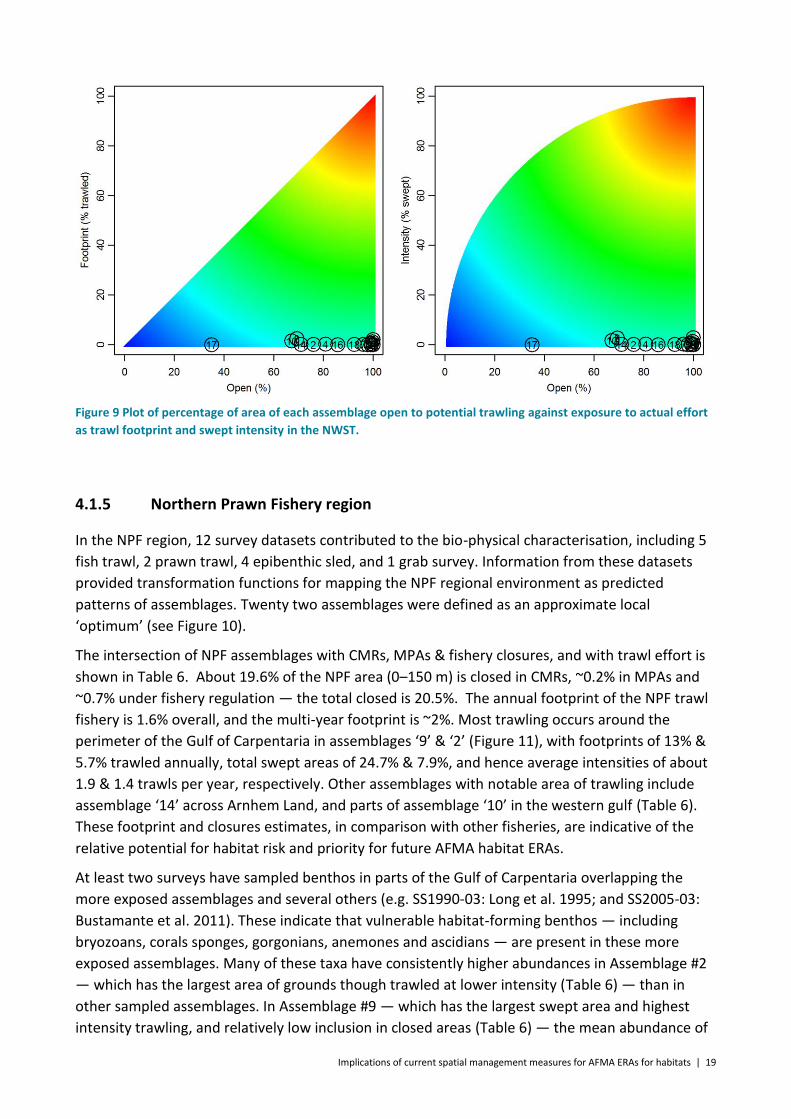
Figure 9 Plot of percentage of area of each assemblage open to potential trawling against actual
exposure to trawl effort intensity in the NWST. ................................................................................ 19
Figure 10 Map of the NPF region showing clustered patterns of species composition change
predicted by relationships with multiple environmental gradients. The biplot shows the first 2
dimensions of the clustered multi-dimensional biological space, representing composition

vi | Implications of current spatial management measures for AFMA ERAs for habitats
change in relation to vectors of the major environmental drivers. The clustering of the
biological space suggests 22 assemblages. ........................................................................................ 20
Figure 11 Plot of percentage of area of each assemblage open to potential trawling against
actual exposure to trawl effort intensity in the NPF. ........................................................................ 21
Figure 12 Map of the TSPF region showing clustered patterns of species composition change
predicted by relationships with multiple environmental gradients. The biplot shows the first 2
dimensions of the clustered multi-dimensional biological space, representing composition
change in relation to vectors of the major environmental drivers. The preliminary clustering of
the biological space suggests 5 assemblages. ................................................................................... 22
Figure 13 Plot of percentage of area of each assemblage open to potential trawling against
actual exposure to trawl effort intensity in the TSPF. ....................................................................... 23
Figure 14 Map of the BSCZS area showing clustered patterns of species composition change
predicted by relationships with multiple environmental gradients. The biplot shows the first 2
dimensions of the clustered multi-dimensional biological space, representing composition
change in relation to vectors of the major environmental drivers. The clustering of the
biological space suggests 11 assemblages. ........................................................................................ 23
Figure 14 Map of all Commonwealth trawl fisheries jurisdictions (<1500 or <150 as
appropriate), showing overall relative exposure of mapped demersal assemblages. Inset: colour
scale indicating assemblage exposure, as used in previous figues. .................................................. 25
Figure 15 Boundaries of Commonwealth demersal trawl fisheries, with bathymetry contours (—
1500m), indicating scope of the project. ........................................................................................... 36
Figure 16 Existing available fish trawl datasets comprising primarily larger species of fishes. ........ 36
Figure 17 Existing available prawn trawl datasets comprising smaller species of fishes and
mobile invertebrates. ......................................................................................................................... 37
Figure 18 Existing available epibenthic sled datasets comprising mobile and sessile
invertebrates. ..................................................................................................................................... 37
Figure 19 Maps of updated the Ocean Colour derived variables, at 0.01° resolution. ..................... 42


2 | Implications of current spatial management measures for AFMA ERAs for habitats
Acknowledgments
This project was supported by funding from the CSIRO and the FRDC on behalf of the Australian
Government.
A steering committee with membership comprising AMFA staff and CFA members provided valued
guidance and feedback to the project.
The CERF Marine Biodiversity Hub provided the initial collation and mapping of national
environmental variables; collation of many of the regional scale demersal biological surveys; and
development of the approach used to predict and map assemblages. The NERP Marine
Biodiversity Hub Project 2.3.2 originally developed the approach applied here for quantifying
exposure of assemblages to trawling.
Updated ocean colour data was sourced from the Integrated Marine Observing System (IMOS),
which is supported by the Australian Government through the National Collaborative Research
Infrastructure Strategy and the Super Science Initiative.
The sources of biological survey datasets as listed in Appendix 3 are acknowledged.

Implications of current spatial management measures for AFMA ERAs for habitats | 3
Executive Summary
In this project, CSIRO researchers implemented the first Australia-wide spatial approach to quantifying the exposure of mapped seabed assemblages to the footprints of Commonwealth demersal trawl fisheries, as well as their spatial protection in areas closed to trawling. These outputs are assisting AFMA in understanding the contributions of existing spatial management measures to environmental sustainability, and to identify and prioritise any remaining needs for addressing risks to habitats. The focus provided by these priorities is intended to reduce the costs of environmental assessments, ultimately having outcomes including reduction of the ecological risks posed by trawling and enhanced environmental sustainability. Trawling footprints were mapped from fishery effort data for recent years. Protection provided by current spatial management included fishery closures, the Commonwealth Marine Reserve system (CMRs), and some other Marine Protected Areas (MPAs). Seabed assemblages — as surrogates for broad habitats — were defined and mapped using a single consistent method that had not been possible previously, but was now enabled by new advances in analyses and the availability of new data & knowledge. The overlaps of each assemblage with trawl footprints, and with areas closed to trawling, were calculated to quantify trawl exposure and spatial protection.
Background To date, ecological risk assessments (ERAs) for Australian trawl fisheries have largely focussed on bycatch and by-product species — and management responses (ERM) have focused on species assessed as being at high risk. However, research has demonstrated that towed demersal fishing gears can impact seabed habitats, which consequently may be at risk. Most fisheries lack adequate data for habitat ERAs, but in some Commonwealth fisheries, initial ERAs identified the nature & diversity of habitats and potential risks from different fishing gears, though could not map spatial extent of habitats and were interim in nature. Subsequently, new management has been implemented — including effort reductions and closures — that may have reduced the level of potential risk. Thus, AFMA has identified the need to extend the ERAs covering habitats, and to take into account the recent management. Specifically, AFMA’s stated priority was a gap analysis to determine the extent to which individual fishery ERAs, and hence ecological risk management (ERM), need to address habitats considering other fishery management measures now in place and following the finalisation of the CMRs network. It is this priority that this project addressed, utilizing new data and spatial mapping methods, for all Commonwealth demersal fisheries that use towed bottom-contact gear (trawls, dredges) in Australian continental shelf and slope waters.
Aims The project aimed to quantify the overlap of mapped seabed assemblages with trawl footprints, and with areas of spatial management that exclude trawling, by building on previously collated data and assemblage mapping — as well as data for Commonwealth demersal trawling effort, fishery closures and marine reserves. These trawl exposure and protection estimates provide information that AFMA can use to focus on priorities or gaps, regarding the needs for any future for habitat ERAs, in their progress towards ecosystem based management.
Methods Most fisheries lacked data for seabed habitats per se. Hence, as surrogates for habitats at meso-scales, assemblages were defined where each represented an area having similar environmental conditions and expected to have a similar mix of fish & invertebrate species. This process built on the foundation provided by significant previous investment in a number of completed and other current projects, but also required collation of additional biological survey datasets and environmental layers, as well as additional data for trawl effort distribution and intensity, and for fishery closures, CMRs and other MPAs. The multiple biological survey datasets were analysed with the environmental layers to quantify the magnitude of change in demersal species composition along the environmental gradients (as predictors). This information was then used to predict and map the distribution of demersal assemblages on a 0.01° grid. Trawled-area footprints were estimated from logbook or VMS effort data for a 3–5 year period post-2007 (after significant restructuring had been implemented in several fisheries) and mapped on the 0.01° grid, as were fishery closures and CMRs. The overlap of each assemblage with trawling and closed areas was then quantified by area and as a percentage. All CMRs

4 | Implications of current spatial management measures for AFMA ERAs for habitats
were assumed to exclude trawling, although most CMR management plans were under review. The fisheries assessed were: Southeast Commonwealth Trawl Sector, Bass Strait Central Zone Scallop (dredge) Fishery, Great Australian Bight Trawl Fishery, Western Deepwater Trawl Fishery, Northwest Slope Trawl Fishery, Northern Prawn Fishery, and Torres Strait Prawn Fishery. Each fishery was analysed separately within its respective management jurisdiction boundary, subject to a maximum depth of 1500 m for fish trawl fisheries and 150 m for prawn and scallop.
Key findings The majority of the 106 seabed assemblages defined and mapped had little or no exposure to trawling by the Commonwealth trawl fisheries assessed. These assemblages with low trawl exposure included a large number with little or no protection in closed areas, in addition to those with high levels of protection in closures. Across all fisheries, there were relatively few assemblages that had both high exposure to trawling and low protection by closed areas. Several more highly exposed assemblages also had substantive inclusion in closed areas. For example, five assemblages had >20% annual trawl footprint exposure (maximum annual footprint = 43.7%), of which two had >20% protection in areas closed to trawling. Those assemblages with both high exposure and low protection may be considered higher priority for future AFMA habitat ERA focus, whereas those with low exposure and high protection may receive less ERA focus. The identification of these assemblages does not necessarily imply actual risk to habitat, but rather, information on the extent of any vulnerable habitats or biological components in the higher priority assemblages is required to make such a risk assessment.
Implications for stakeholders It is likely that the majority of demersal assemblages within these Commonwealth trawl fishery jurisdictions are not subject to substantive risk from these fisheries, due to their low exposure, and this is largely independent of whether assemblages have high or no protection. The relatively few assemblages within these jurisdictions that have higher exposures to trawling may have potential for risk to vulnerable habitats if such habitats occur in these areas. Thus, the limited resources for future habitat ERAs can be focussed on the small number of more highly exposed assemblages, particularly those with lower levels of protection, to assess whether vulnerable habitats are present and whether they are at substantive risk from demersal trawl or dredge fishing. This focus will enable more efficient application of resources on environmental risk assessments for habitats. Ultimately, expected benefits include reduction in environmental risks due to trawling, and hence AFMA meeting requirements of legislation regarding environmental sustainability, and improved social licence for fisheries.
Recommendations Decisions regarding the final priorities for future habitat risk assessments should include further discussions with AFMA, industry associations and industry members of relevant fisheries, AFMA’s consultative management and scientific committees, and researchers. The discussions should also include potential methods that may be suitable for determining whether sensitive habitats or habitat-forming biological components are present in the priority assemblages, and for assessing whether they are at substantive risk from trawling. The priorities for future habitat ERAs need to account for the uncertainties inherent in mapping assemblages and trawl footprints.
The project scope was Commonwealth trawl & dredge fisheries only — it did not map assemblages outside of these jurisdictions or address the footprints of State bottom-trawl fisheries. This may be significant because, although State trawl fisheries generally occur outside Commonwealth jurisdictions, some assemblages extend outside of these jurisdictions and may be exposed to State trawl fisheries. In addition, some State fisheries operate within the jurisdictional boundaries of some Commonwealth trawl fisheries. This may affect the relative priorities of assemblages determined by this project. Further, it is now feasible to apply the approach used in this project to all Australian fishery jurisdictions and cover State managed fisheries, to provide a single consistent national assessment of the exposure of assemblages to trawling, with an ultimate expected outcome of leading to achievement and demonstration of habitat sustainability for all Australian demersal trawl fisheries.
Keywords ecological risk assessment; ERA; bottom trawling; effects of trawling; trawl impacts; seafloor damage; trawl footprints; seabed assemblages mapping; marine protected areas; marine parks.

Implications of current spatial management measures for AFMA ERAs for habitats | 5
1 Introduction
Australia is a world leader in ecosystem based management of fisheries; nevertheless, addressing
the environmental sustainability of fishing continues to be a major strategic challenge. Australian
fisheries must meet legislative requirements under the Environmental Protection & Biodiversity
Conservation (EPBC) Act and regular environmental reviews assessed by the Department of
Environment (DoE). In response to the EPBC Act, related regulations and international obligations,
the Australian Fisheries Management Authority (AFMA) has for some time been moving beyond
target species to take an ecosystem-based approach to managing Commonwealth fisheries, aiming
for broader environmental sustainability including for bycatch species, habitat and communities.
Typically, a risk assessment approach is being taken for this purpose.
CSIRO, among others, has been supporting AFMA and other management agencies to meet these
requirements for several years. For example, with ecological risk assessments (ERAs) for species,
bycatch, habitats and communities (e.g. Stobutzki et al. 2000, 2001; Pitcher et al. 2007ab; Pitcher
2013, 2014, 2015; Hobday et al. 2011ab; Zhou et a. 2009). Much of this effort has been focussed
on bycatch, and ERAs for bycatch species have been conducted for most Commonwealth fisheries.
However, research has demonstrated that demersal towed fishing gears can impact seabed
habitats and communities (e.g. Burridge et al. 2003; Pitcher et al. 2016), which consequently are
considered potentially at risk. Accordingly, ERAs for habitats have been completed, at a qualitative
level, for some Commonwealth fisheries (e.g. Williams et al. 2011). Nevertheless, largely due to
inadequate data for most fisheries, most habitat ERAs were non-spatial (i.e. the spatial extent of
risk was unknown) and interim in nature.
More recently, new data and methods have become available that permit an advancement of
these assessments; and further, new management has been implemented — including effort
management, fishery closures and the Commonwealth Marine Reserve system (CMRs) — that may
change the spatial extent of potential risk to habitats from trawling. Thus, AFMA has identified a
need to extend the ERAs covering habitats and communities, taking into account the new
management, information and methods. In particular, AFMA has specified a priority requirement
for a gap analysis to determine the extent to which individual fishery ERAs, and hence ecological
risk management (ERM), need to address habitats considering other fishery management
measures now in place — including effort reductions & closures — and following the finalisation of
the CMRs network. It is this priority need that this project was specifically developed to address.
In addition to the new management, the project also took into account the new data &
knowledge, and new advances in methods, to implement a consistent national-scale assemblage
mapping approach that had not been possible previously, and applied it to Commonwealth
demersal trawl fisheries. The scope included Australian continental Commonwealth demersal
fisheries that use towed bottom-contact gear in shelf and mid/upper-slope waters. These fisheries
included: the Southeast Commonwealth Trawl Sector (SET), the Great Australian Bight Trawl
Fishery (GABTF), the Western Deepwater Trawl Fishery (WDTF), the Northwest Slope Trawl Fishery
(NWSTF), the Northern Prawn Fishery (NPF), the Torres Strait Prawn Fishery (TSPF) and the Bass
Strait Central Zone Scallop (dredge) Fishery (BSCZS). Each fishery was analysed separately within
its respective management jurisdiction boundary, subject to a maximum depth of 1500 m for fish
trawl fisheries and 150 m for Prawn (NPF, TSPF) and Scallop (BSCZS) (see Appendix 1).

6 | Implications of current spatial management measures for AFMA ERAs for habitats
2 Objectives
Build on recently collated data and mapped distributions of predicted demersal assemblages — as
well as data for Commonwealth demersal fishing effort, fishery closures and marine reserves — to
provide:
- quantification of the overlap of current fishing effort and intensity with each mapped
assemblage,
- quantification of the overlap of each mapped assemblage with areas of spatial management
that exclude fishing, such as fishery closures and marine reserves,
- a gap analysis and prioritisation of which mapped assemblages, and in which fisheries, may
require future focus for AFMAs fishery ERAs.
- qualitative assessment of the potential risk implications for any habitat forming biota (if/where
data available) in mapped assemblages with high exposure to fisheries, given current spatial
management.
3 Methods
The project built on the foundation provided by significant previous investment in a number of
completed and current projects that provided: the underpinning methods for high-resolution
regional-scale quantitative risk assessments of assemblages and habitats (e.g. the “GBR Seabed
Biodiversity Project”, Pitcher et al. 2007a); a comprehensive database of available demersal
biodiversity survey datasets and environmental data layers with national coverage, new methods
for predicting patterns of biodiversity composition at regional scale from multiple disparate inputs,
and maps of predicted assemblages for each large marine planning region nationally (the CERF
Marine Biodiversity Hub “Prediction Program”, Pitcher et al. 2011); updated biological survey and
environmental datasets and revised regional maps of predicted seabed assemblages (CERF
Transition Program “New data layers”, McLeod & Pitcher 2011); compilations of Commonwealth
fishing effort and closures information, and development of the assemblages overlap approach to
be used in this project (NERP Marine Hub Project 2.3.2 “Landscape approach to supporting
management of benthic biodiversity in the Southeast Marine Region”, Pitcher et al. 2015). These
existing data, including fishing effort, had already been mapped to a common 0.01° (~1.11 km)
grid and were re-used by this project.
The existing predicted large marine region (LMRs) assemblage maps (e.g. Ellis & Pitcher 2009abc,
2010, 2011; Pitcher et al. 2011), fishing effort data and closures information from these projects
provided the basis for the assessments reported here. However, the specific purposes of the
current project — i.e. assemblage maps that matched each fishery jurisdiction specifically (rather
than the LMRs) to ensure that assessments were appropriate and valid to relevant stakeholders —
required re-assembly of datasets and re-analysis. In addition, the earlier coarse-resolution NASA-
sourced ocean colour data were updated with a higher resolution (0.01°) product provided by the
Integrated Marine Observing System (IMOS); and a number of additional biological survey

Implications of current spatial management measures for AFMA ERAs for habitats | 7
datasets were acquired and included in analyses. The assemblage maps provided meso-scale
surrogates for habitats, given the lack of data for seabed habitats per se in most fisheries. Each
assemblage represents an area expected to have a similar mix of species that differs from
neighbouring assemblages and increasingly to more distant assemblages.
3.1 Datasets
3.1.1 Biological survey datasets
Many existing biological datasets (about 20) for large scale surveys suitable for the project were
available from previous projects (e.g. collated the CERF Marine Hub Prediction Program, Pitcher et
al. 2011, see Appendix 2). These primarily include fish trawls comprising mostly larger species of
fishes. For parts of Australia, there are also prawn trawl surveys that include smaller species of
fishes and mobile invertebrates. In some regions there were also epibenthic sled datasets that
include mobile and sessile invertebrates. A few regions also had infaunal grab data (e.g. Gulf of
Carpentaria).
Additional biological survey datasets collated recently and/or by this project include:
- Museum Victoria Bass Strait Survey (epibenthic sleds and grabs: Wilson & Poore 1987; O’Hara
2002);
- Western Australian Department of Fisheries Shark Bay and Exmouth Gulf Biodiversity survey
(prawn trawls: Kangas et al. 2007);
- SARDI Eastern Great Australian Bight Benthic Protection Zone surveys (epibenthic sleds and
grabs: Ward et al. 2003; Currie et al. 2007, 2008);
- CSIRO Western Australian Slope Voyage of Discovery (beam trawls, sleds & grabs: Alan
Williams et al, unpubl.);
- Northern Territory Fisheries Groundfish Stock Survey, 1990 & 1992 (fish trawls: Ramm 1997).
- SET and GAB Fishery Independent Survey (FIS) datasets (Ian Knuckey et al. unpubl., Fishwell
Consulting/AFMA).
These datasets were checked, cleaned and re-formatted to be compatible with existing survey
datasets and with the analyses procedures.
A full list of biological survey datasets used by the project is shown in Appendix 3.
3.1.2 Mapped environmental predictors
About 26 environmental variables were collated and mapped at 0.01° for the Australian EEZ by the
CERF Marine Biodiversity Hub, for the purpose of biodiversity distribution analysis and prediction
(Huang et al. 2011; Pitcher et al. 2011; see variables #1–26 in Appendix 4). Subsequently,
additional variables were collated (#27–40) as part of the CERF Hub Transition program (McLeod &
Pitcher 2011) and/or the NERP Marine Hub (Pitcher et al. 2015). The original 0.1 degree seabed
stress layer was replaced by higher resolution national data layer from the CSIRO ‘Ribbon Model’
(#8).

8 | Implications of current spatial management measures for AFMA ERAs for habitats
The Ocean Colour derived variables (#21–34, Appendix 4), originally from NASA sources at ~0.1
degree, were updated to higher resolution 0.01° products from IMOS for variables #21–30
(Appendix 4). From these, the data for the Australian EEZ were extracted and the ‘climatological’
annual average & seasonal range were calculated, as well as the further derived variables #31–34
(Appendix 4). Updated maps for these Ocean Colour variables are shown in Appendix 6.
A complete list of mapped environmental variables used by the project is shown in Appendix 4,
including full definitions, abbreviations and sources.
3.1.3 Closures and Marine reserves
Data on SESSF permanent fishery closures, and Commonwealth Marine Reserves (CMRs), were
largely available from previous recent projects (e.g. Pitcher et al. 2015). Additional data for
closures (permanent only) in other Commonwealth fisheries (e.g. NPF, TSPF), and for other Marine
Protected Areas, were collated by this project (see Appendix 5). All were mapped to the 0.01° 0–
1500 m database and analysis grid to be used by this project (Figure 1).
200 m
1500 m
Figure 1 Commonwealth demersal fishery areas (blue), CMR’s & MPA’s (green) and closures (dark grey/black) for
fish & prawn trawl and scallop dredge. Areas in-scope for study (<1500m/150m) in dark colours (blue, green, black,
brown=CMR & Closure, magenta=MPA & Closure).
All CMRs were assumed to exclude trawling, as intended when boundaries were declared. We
note that management plans within CMR boundaries (except southeast) are currently under
review, and permitted activities within CMRs were not finalised during this project.
NWSTF
NPF
WD TF
SESS GAB
TSPF
BSCZS
SET

Implications of current spatial management measures for AFMA ERAs for habitats | 9
3.1.4 Trawl effort data
Data on annual trawl effort gridded at 0.01° were available from previous recent projects, where
they were sourced from logbook records or VMS data, as available for each fishery (see Appendix
5), linear interpolated between tow start-end positions or successive trawl polls and aggregated to
grids. For this project, effort data were extracted for each fishery for a recent period of 3–5 years,
typically post-2007, to account for significant recent management changes in several fisheries. In
all fisheries, trawl effort and footprints had been greater in previous years; however, only current
effort levels were within the project scope. Effort in various metrics (hours, metres, number of
tows, etc) were all converted to swept-area per grid-area ratio, to standardise for different gear
sizes and tow speeds. The annual average for each grid was taken to define the typical spatial
distribution of trawl intensity for recent years in each fishery. The effort data was joined to the
gridded environmental variables for each fishery and mapped.
The current footprints for each fishery were estimated (Table 1). These show the total area of each
fishery within the specified depth-range, the total area of 0.01° grid cells with trawling recorded in
recent years, the total swept-area of all trawls annually, the footprint area accounting for
overlapping effort in grid cells with swept-area ratio >1 assuming trawling is conducted uniformly
at 0.01° scale, and the footprint area accounting for overlapping effort within grid cells assuming
trawling is conducted randomly at sub-0.01° scale. The random <0.01° estimates the annual
average footprint. However, among years the fine distribution of trawling at 10–100 m scales is
not exactly the same, and over multiple years the footprint tends to approximate the uniform
footprint. The estimated annual footprints range from <1% to ~8% of the managed area of each
fishery within the specified depth range, whereas the multi-year footprints typically are about 25%
larger. Both estimates account for the aggregated nature of trawling at ~1–10 km scales.
Table 1 Footprints (km²) of Commonwealth demersal trawl fisheries, for depth range 0–1500 m (or 0–150 m).
FISHERY TOTAL GRID AREA TOTAL WITH TRAWL TOTAL SWEPT AREA UNIFORM @ 0.01° (%) RANDOM < 0.01° (%)
SET Fishery 227,255 71,633 33,403 21,356 (9.4) 17,312 (7.6)
NPF Fishery 749,629 67,949 19,913 15,012 (2.0) 12,175 (1.6)
GAB Fishery 157,335 24,218 10,195 7,745 (4.9) 6,042 (3.8)
TSPF Fishery (0–150m) 36,168 4,690 2,682 1,773 (4.9) 1,414 (3.9)
NWST Fishery 180,977 8,579 1,018 992 (0.5) 855 (0.5)
WDT Fishery 154,655 3,385 300 294 (0.2) 243 (0.2)
BSCZ Fishery (0–150m) 75,084 680 24 24 (<.1) 22 (<.1)
3.2 Analyses
The approach for producing the assemblage maps is now established; it involves quantifying the
magnitude of change in species composition along environmental gradients (predictors) and using
this information to predict distribution patterns of demersal biodiversity. The method, called
“Gradient Forest" (Ellis et al. 2012), is an extension of Random Forest (Breiman 2001), which fits
an ensemble of bootstrapped regression tree models (a ‘forest’ — of 500 trees in our case)

10 | Implications of current spatial management measures for AFMA ERAs for habitats
between each individual species abundance and environmental variables. The many branches (or
‘splits’) in the tree models are fitted recursively along the environmental gradients at locations on
variables where the most deviance in species response is explained (fit ‘improvement’). Each tree
is fitted to a different random sample of ~⅔ of the data (in-bag) and fit performance is tested on
the ~⅓ of data held out-of-bag (OOB). The influence of each variable was assessed by randomly
permuting each variable in turn and quantifying the degradation in prediction performance on the
OOB data (‘predictor importance’). Models were fitted for every species with adequate occurrence
in every available biological survey dataset.
From the Random Forest models, Gradient Forest extracts each split value and deviance
improvement. The split-improvements were aggregated and standardised by data density to
quantify where species composition changes occurred along the gradients. Cumulative
distributions of the splits on each predictor represent overall changes in the whole community, or
compositional turnover, in standardised units of R² along the gradient of each predictor. These
turnover curves are accumulated for the fishery region to provide empirical functions for
transforming the multi-dimensional environmental gradients to common biologically-scaled axes
that can be used to estimate the spatial pattern of species composition — or assemblages —
associated with the environment and mapping in geographic space. Because these functions
integrate biological information, they provide improved use of environmental variables as
surrogates for predicting and mapping patterns of biodiversity. The method has been used to
produce biodiversity and bioregional maps in Australia and overseas. Statistical details of Gradient
Forest are described in Ellis et al. (2012), and example ecological applications are described in
Pitcher et al. (2010, 2012); further information is available at http://r-forge.r-
project.org/projects/gradientforest/.
After the multiple environmental gradients have all been transformed to a common biological
scale, principal components analysis (PCA) is used to capture the majority of compositional
variation associated with environmental gradients in as few dimensions as possible. A colour ramp
is applied to the PCA ordination (e.g. red-green-blue in three dimensions, or a colour wheel
around the first two dimensions) to allow visualisation of compositional patterns in 2-D PCA-space
and in mapped geographic space. The visualisation in PCA-space may be called ‘biological-space’
— it is a ‘bi-plot’, with vectors showing the direction of the major environmental drivers, and
provides a colour key for the corresponding geographic map to facilitate interpretation.
In this application, the continuous variation in composition in biological space was clustered to
represent expected species-assemblage groups, which were also mapped in biological space and
geographic space. Determining the most appropriate number of clusters, or predicted
assemblages, for a region is non-exact — several guides have been trialled previously (Pitcher, Ellis
& Dunstan 2011). This number should be guided by the original biological survey data as much as
possible, although this is not straightforward for the case of several contributing surveys each
having only partial coverage of a region. A two-step approach was taken. First, multivariate
regression trees (MRT) were applied to each biological survey separately to obtain an objective
number of clusters (i.e. terminal nodes) for sampled sites in each dataset by partitioning on
environmental variables using cross-validation. The resulting number of terminal nodes sets a
minimum constraint on the number of clusters in biological space; i.e. the number of clusters in
the whole region must be sufficient to split each set of survey sites into at least the number of
MRT terminal nodes. The second step assessed which regional clustering — over a plausible range

Implications of current spatial management measures for AFMA ERAs for habitats | 11
of numbers of clusters — taken as a factor, accounted for most variation in the constituent
biological survey datasets. This involved linking each candidate clustering back to the biological
data using multivariate analysis of variance method (distance-based redundancy analysis, db-RDA,
Legendre and Anderson 1999). The db-RDA provides a multivariate F-ratio test statistic, a large
value of which would indicate evidence that a given clustering has captured structure in the survey
sample data. The F-ratio for each survey in the region was obtained, and the geometric mean of
these was used as the diagnostic. Subject to the step one minimum constraint, the clustering with
the largest mean F-ratio was preferred on biological grounds.
3.3 Assessments
Each mapped assemblage provided the basic unit of assessment and after the assemblage maps
and trawl effort & closures datasets were produced for each Commonwealth fishery jurisdiction,
the quantitative overlap assessments comprised relatively straightforward spatial analyses. First,
the various types of spatial management, including Commonwealth marine reserves, other marine
protected areas, and fishery closures (Figure 1) were overlaid on the assemblage maps and the
area of each mapped assemblage represented in each category of spatial management was
quantified by area and as a percentage. Where possible, reserves were categorised using the IUCN
framework. Second, the annual trawl footprint of each demersal fishery (see Table 1 ‘random’)
was overlaid on the corresponding assemblage map, and the extent of footprint overlap on each
assemblage was quantified by area and as a percentage. The multi-year footprint area (Table 1
‘uniform’) was also estimated — these typically were about 25% larger than annual footprints. As
an indicator of trawl effort intensity, the total swept area in each assemblage was also quantified
by area and as a percentage. This information was tabulated for each assemblage in each fishery.
The level of exposure of each assemblage to trawling, and protection in spatial management, was
also plotted for each fishery in a format analogous to previous ERA presentations.
To provide an overall synthesis, all mapped assemblages were ordered by exposure to trawling
and (inverse) overlap in fishery closures and reserves. This ordered list is provided to support
prioritisation for AFMA decision making regarding the identity and requirement for any
assemblages to be the focus of future ERAs for habitat.
The trawl footprint exposure of assemblages is an indicator of potential risk but is not directly an
assessment of risk of trawl impacts on habitats per se. Where possible, for any assemblages that
appeared to be of higher priority — if suitable information was available — the potential risk
implications were discussed with reference to the impact/recovery attributes of the constituent
habitat forming biota, similarly to previous qualitative habitat ERAs.
4 Results & Discussion
4.1 Analyses & assessments
Analyses of biological survey data, mapping of assemblages, and overlap assessments were
completed for six Commonwealth trawl fisheries: SESS CTS (SET) and GAB, WDTF, NWSTF, NPF,
TSPF, and the BSCZS dredge fishery (see Appendix 1).

12 | Implications of current spatial management measures for AFMA ERAs for habitats
4.1.1 South East Trawl Fishery region
In the SET region, 14 datasets contributed to the assemblage characterisation, comprising 8 fish
trawl (including Fishery Independent Surveys, FIS), 4 benthic sled, 1 grab survey, and 1 aggregated
video dataset. The combined information from these datasets provided functions for transforming
the SET regional environment to a multi-dimensional biological space, and mapping in geographic
space (Figure 2 inset). From this map of continuous compositional change, a set of assemblages
were defined. While defining the appropriate number of assemblages for a region is non-exact,
here a local ‘optimum’ at 20 assemblages has been selected — based on the maximum F-ratio
statistic for a multivariate analysis of variance method (see Methods) — and mapped (Figure 2).
Figure 2 Map of the SET region showing patterns of species composition change predicted by relationships with
multiple environmental gradients, clustered into 20 assemblages. The inset map shows continuous patterns of
composition prior to clustering. The two biplots show the first 2 dimensions of the clustered multi-dimensional
biological space, representing composition change in relation to vectors of the major environmental drivers.

Implications of current spatial management measures for AFMA ERAs for habitats | 13
The intersection of the mapped assemblages with CMRs & fishery closures, and with trawl effort
was then estimated (Table 2). About 8.5% of the SET area (0–1500 m) is closed in CMRs, and 41.3%
is trawl fishery closures — together, with overlaps, 46.7% is closed. In the case of trawl effort,
trawl “Grounds” refers to the total area of 0.01° grid cells with any trawling recorded in recent
years; “Uniform” refers to the trawl footprint area assuming trawling is conducted uniformly at
0.01° scale and such that overlapping effort in grid cells with swept-area ratio >1 is accounted for;
“Random” is the footprint area accounting for overlapping effort within grid cells assuming
trawling is conducted randomly at sub-0.01° scale; and “Trl swept” is the total swept area of
trawling within each assemblage and is an indicator of the intensity of trawling on the trawl-
exposed portion of each assemblage — typically, the exposed portions are trawled with an
average intensity of about twice annually. The random area estimates the annual footprint of
trawling at 7.7% across the entire region, whereas the uniform area estimates the multi-year
footprint of trawling at 9.5%.
The percentage of each assemblage included in closed areas and that exposed to trawl footprint,
as well as total swept area, are factors that influence the potential for habitat risk and hence the
priority for future AFMA habitat ERAs. These are plotted in Figure 3. Note that area open and area
of trawl footprint cannot sum to more than 100% of an assemblage, whereas total swept area
could be greater than the open area of an assemblage (potentially >100%). The most exposed
assemblage is Assemblage #20 on the shelf off southern NSW/eastern Victoria (Figure 2) with an
annual footprint of 43.7% and total swept area of 76.3% suggesting an average intensity of ~1.75
trawls per year in exposed areas — it also has the least overlap in closed areas (0.9%). Other
exposed assemblages include #4 on the slope off the Bonney Coast, followed by assemblages #1
on the NSW shelf and #2 on the outer shelf and slope beyond assemblage #20.
Table 2 Intersection of Assemblages by area, in the SET region, with CMRs and fishery closures (and both
combined), and with trawl effort. Note, colours are simply to highlight relatively high & low numbers in each
column, and do not imply any ‘traffic-light’ style ‘report card’ against particular benchmarks. Green indicates
relatively high overlap in closed areas; Blue indicates relatively low overlap with trawling.
Assemblage Grid count Area(km²) CMR_IA CMR_II CMR_VI CMRs % CMR MPAs Closures %Closed Any Clsd Total%Clsd Grounds Uniform Random % Trawled Trl Swept % Swept
1 9,139 9,271 264 264 2.9 0 999 10.8 1,258 13.6 7,676 2,816 2,313 24.9 4,557 49.2
2 7,040 6,792 18 371 389 5.7 0 2,234 32.9 2,281 33.6 5,449 1,827 1,463 21.5 2,706 39.8
3 3,068 3,097 518 518 16.7 0 2,001 64.6 2,128 68.7 1,178 43 42 1.4 43 1.4
4 5,846 5,655 72 72 1.3 0 1,510 26.7 1,547 27.4 4,773 2,495 2,051 36.3 4,556 80.6
5 17,656 16,943 1,056 1,056 6.2 0 1,529 9.0 2,586 15.3 5,630 1,003 885 5.2 2,467 14.6
6 13,051 12,158 12 856 867 7.1 0 73 0.6 902 7.4 5,048 517 467 3.8 1,338 11.0
7 15,985 15,140 163 1,115 1,278 8.4 0 6,728 44.4 7,944 52.5 1,788 551 452 3.0 907 6.0
8 8,338 7,796 586 102 398 1,086 13.9 0 4,659 59.8 4,678 60.0 3,803 342 299 3.8 362 4.6
9 8,111 7,790 242 242 3.1 0 5,130 65.8 5,130 65.8 3,641 251 228 2.9 251 3.2
10 16,138 15,261 7 616 623 4.1 0 12,102 79.3 12,679 83.1 752 242 187 1.2 283 1.9
11 16,214 15,383 938 938 6.1 0 10,880 70.7 11,546 75.1 1,807 60 57 0.4 60 0.4
12 24,508 23,388 825 825 3.5 0 11,427 48.9 11,801 50.5 1,796 184 165 0.7 222 0.9
13 12,247 11,690 1,631 1,631 14.0 0 5,352 45.8 6,963 59.6 262 21 19 0.2 49 0.4
14 15,064 13,507 691 23 2,625 3,339 24.7 0 30 0.2 3,346 24.8 6,570 2,089 1,709 12.7 3,268 24.2
15 5,690 5,069 9 1,813 1,822 35.9 0 1,967 38.8 2,093 41.3 1,402 73 69 1.4 74 1.5
16 9,965 9,353 0 0.0 0 9,340 99.9 9,340 99.9 13 5 4 0.0 5 0.1
17 8,834 8,652 0 0.0 0 3,945 45.6 3,945 45.6 3,209 799 686 7.9 1,551 17.9
18 9,116 8,761 601 601 6.9 0 1,204 13.7 1,768 20.2 4,653 748 629 7.2 963 11.0
19 17,471 17,367 3,583 3,583 20.6 0 12,150 70.0 13,522 77.9 186 3 3 0.0 3 0.0
20 13,319 12,970 13 13 0.1 0 112 0.9 122 0.9 12,112 7,386 5,665 43.7 9,899 76.3
236,800 226,043 1,286 326 17,537 19,148 8.5 0 93,372 41.3 105,579 46.7 71,747 21,456 17,393 7.7 33,565 14.8
Recent studies (e.g. Williams et al. 2006 & 2009) have indicated that vulnerable habitat-forming
benthos types are present in these more exposed assemblages. For example, sub-cropping friable

14 | Implications of current spatial management measures for AFMA ERAs for habitats
sandstone supporting gardens of large sponges are restricted within a few exposed mid-shelf
assemblages; aggregations of the relict stalked crinoid Metacrinus cyaneus are restricted within a
few exposed shelf-break assemblages; a ribbon of delicate bryozoan communities occur in a
limited depth range within many shelf-edge assemblages, some of which are exposed; and tree-
forming octocorals and black corals are restricted to high flow, steep banks in upper-slope
assemblages, some of which are exposed. These vulnerable types occur in places potentially
accessible to and removable by trawls and may be at risk (Williams et al. 2011) at least locally
within assemblages, if not at regional landscape scale (Pitcher et al. 2015).
Figure 3 Plot of percentage of area of each assemblage open to potential trawling against exposure to actual effort
as trawl footprint and swept intensity in the SET; diagrammatically illustrating potential for habitat risk and relative
priority for habitat ERA. Note, background colours are simply to highlight relative exposure and do not imply
absolute risk.
4.1.2 Great Australian Bight Trawl Fishery region
For the GAB region, 10 survey datasets contributed to the bio-physical characterisation, including
5 trawl (including FIS), 3 epibenthic sled, and 2 grab surveys. Analyses of these datasets provided
transformation functions for mapping the GAB regional environment as predicted patterns of
assemblages, and 13 assemblages were defined as an approximate local ‘optimum’ (see Figure 4).
The intersection of GAB assemblages with CMRs & fishery closures, and with trawl effort is shown
in Table 3. About 12.3% of the GAB area (0–1500 m) is closed in CMRs, and 11.2% is trawl fishery
closures — together, with overlaps, 21.9% is closed. The annual footprint of the GAB trawl fishery
is 3.8% (random within 0.01° cells), and the multi-year footprint is ~4.9% (uniform within cells).
Assemblage #8, along the shelf-edge/upper slope, is notably more exposed to trawling (~34%
annually; ~59% swept average intensity ~1.74) than all others (Figure 5). These exposure
estimates are indicative of the relative potential for habitat risk within assemblages, and hence
also the relative priority need for future AFMA habitat ERAs. Within assemblage #8, vulnerable
habitat-forming benthos types do occur and are likely to be at risk where trawling occurs (Williams
et al. 2011), but actual risk at larger scale remains to be assessed quantitatively.

Implications of current spatial management measures for AFMA ERAs for habitats | 15
Figure 4 Map of the GAB region showing clustered patterns of species composition change predicted by
relationships with multiple environmental gradients. The biplot shows the first 2 dimensions of the clustered multi-
dimensional biological space, representing composition change in relation to vectors of the major environmental
drivers. The clustering of the biological space suggests 13 assemblages.
Table 3 Intersection of Assemblages by area, in the GAB region with CMRs and fishery closures (and both
combined), and with trawl effort.
Assemblage Grid count Area(km²) CMR_? CMR_II CMR_VI CMRs % CMR MPAs Closures %Closed Any Clsd Total%Clsd Grounds Uniform Random % Trawled Trl Swept % Swept
1 15,353 15,509 1,943 299 2,242 14.5 0 1,713 11.0 3,699 23.9 155 4 4 0.0 4 0.0
2 12,702 12,994 3,346 102 3,448 26.5 0 1,038 8.0 4,385 33.7 144 2 2 0.0 2 0.0
3 15,523 15,870 1,358 252 165 1,775 11.2 0 7,254 45.7 8,285 52.2 353 20 17 0.1 28 0.2
4 5,184 5,239 248 674 922 17.6 0 1,417 27.0 1,997 38.1 34 5 4 0.1 6 0.1
5 12,405 12,677 561 160 306 1,026 8.1 0 3,941 31.1 4,539 35.8 902 30 28 0.2 30 0.2
6 6,928 7,077 177 74 523 773 10.9 0 783 11.1 1,362 19.2 1,542 75 71 1.0 75 1.1
7 13,593 13,886 845 116 507 1,468 10.6 0 1,452 10.5 2,315 16.7 4,480 281 253 1.8 281 2.0
8 15,814 16,280 850 5 46 901 5.5 0 32 0.2 932 5.7 13,545 7,183 5,533 34.0 9,623 59.1
9 14,468 14,953 991 6 6 1,004 6.7 0 0 0.0 1,004 6.7 2,427 131 114 0.8 131 0.9
10 5,977 6,201 1,134 1,134 18.3 0 0 0.0 1,134 18.3 118 2 2 0.0 2 0.0
11 12,300 12,744 783 783 6.1 0 0 0.0 783 6.1 313 6 6 0.0 6 0.0
12 7,776 8,073 3,320 3,320 41.1 0 0 0.0 3,320 41.1 1 1 0 0.0 1 0.0
13 15,028 15,664 596 596 3.8 0 0 0.0 596 3.8 0 0 0 0.0 0 0.0
153,051 157,167 11,206 5,560 2,628 19,394 12.3 0 17,631 11.2 34,351 21.9 24,014 7,738 6,035 3.8 10,188 6.5
Figure 5 Plot of percentage of area of each assemblage open to potential trawling against exposure to actual effort
as trawl footprint and swept intensity in the GAB. Note, background colours are simply to highlight relative
exposure and do not imply absolute risk.

16 | Implications of current spatial management measures for AFMA ERAs for habitats
4.1.3 Western Deepwater Trawl Fishery region
In the WDT region, 10 survey datasets contributed to the bio-
physical characterisation, including 2 fish trawl, 1 beam trawl, 1
prawn trawl, 1 epibenthic sled, and 1 grab survey. Information
from these datasets provided transformation functions for
mapping the WDT regional environment as predicted patterns of
assemblages. Fourteen assemblages were defined as an
approximate local ‘optimum’ (see Figure 6).
Figure 6 Map of the WDT region showing clustered patterns of species
composition change predicted by relationships with multiple environmental
gradients. The biplot shows the first 2 dimensions of the clustered multi-
dimensional biological space, representing composition change in relation to
vectors of the major environmental drivers. The clustering of the biological
space suggests 14 assemblages.
The intersection of WDT assemblages with CMRs & fishery
closures, and with trawl effort is shown in Table 4.
Table 4 Intersection of Assemblages by area, in the WDT region with CMRs and fishery closures (and both
combined), and with trawl effort.
Assemblage Grid count Area(km²) CMR_IA CMR_II CMR_VI CMRs % CMR MPAs Closures %Closed Any Clsd Total%Clsd Grounds Uniform Random % Trawled Trl Swept % Swept
1 7,588 8,509 0 0.0 0 0 0.0 0 0.0 0 0 0 0.0 0 0.0
2 17,659 19,053 794 244 3,113 4,151 21.8 0 0 0.0 4,151 21.8 112 2 2 0.0 2 0.0
3 17,170 19,950 3,574 3,574 17.9 0 0 0.0 3,574 17.9 0 0 0 0.0 0 0.0
4 12,403 13,509 138 127 2,477 2,742 20.3 0 0 0.0 2,742 20.3 105 2 2 0.0 2 0.0
5 7,457 8,461 1,121 1,121 13.2 0 0 0.0 1,121 13.2 35 1 1 0.0 1 0.0
6 7,270 8,186 46 46 0.6 0 0 0.0 46 0.6 11 0 0 0.0 0 0.0
7 6,893 7,481 134 971 1,105 14.8 0 0 0.0 1,105 14.8 81 2 2 0.0 2 0.0
8 5,267 5,942 129 364 493 8.3 0 0 0.0 493 8.3 387 9 9 0.2 9 0.2
9 7,814 8,355 84 1,438 1,522 18.2 0 0 0.0 1,522 18.2 742 103 82 1.0 107 1.3
10 4,220 4,709 277 399 676 14.4 0 0 0.0 676 14.4 1,625 165 136 2.9 167 3.6
11 30,188 34,872 13,439 13,439 38.5 0 0 0.0 13,439 38.5 22 1 1 0.0 1 0.0
12 3,436 3,958 108 742 850 21.5 0 0 0.0 850 21.5 0 0 0 0.0 0 0.0
13 6,797 6,960 2,438 2,438 35.0 0 0 0.0 2,438 35.0 0 0 0 0.0 0 0.0
14 4,205 4,316 170 837 1,007 23.3 0 0 0.0 1,007 23.3 23 1 1 0.0 1 0.0
138,367 154,260 1,834 371 30,958 33,163 21.5 0 0 0.0 33,163 21.5 3,143 287 237 0.2 293 0.2

Implications of current spatial management measures for AFMA ERAs for habitats | 17
About 21.5% of the WDT area (0–1500 m) is closed in CMRs, and none is closed under fishery
regulation — so the total is 21.5% closed. The annual footprint of the WDT trawl fishery is 0.16%
overall, and the multi-year footprint is ~0.19%, with most trawling along the shelf-edge/upper
slope in assemblage ‘10’ (Figure 7). Compared with other Commonwealth fisheries, these
estimates are indicative of relatively low potential for habitat risk and priority for future AFMA
habitat ERAs.
Figure 7 Plot of percentage of area of each assemblage open to potential trawling against exposure to actual effort
as trawl footprint and swept intensity in the WDT.
4.1.4 Northwest Slope Trawl Fishery region
In the NWS region, 10 survey datasets contributed to the bio-physical characterisation, including 7
fish trawl, 1 beam trawl, 1 epibenthic sled, and 1 grab survey. Information from these datasets
provided transformation functions for mapping the NWSF regional environment as predicted
patterns of assemblages. Twenty one assemblages were defined as an approximate local
‘optimum’ (see Figure 8).
The intersection of NWS assemblages with CMRs, MPAs & fishery closures, and with trawl effort is
shown in Table 5. About 12.1% of the NWS area (0–1500 m) is closed in CMRs, none in MPAs or
under fishery regulation — the total closed is 12.1%. The annual footprint of the NWS trawl
fishery is 0.47% overall, and the multi-year footprint is ~0.54%, with the trawling that does occur
primarily located below the shelf break in assemblages ‘5’ and ‘8’ (Figure 9). These footprints are
indicative of relatively low potential for habitat risk and priority for future AFMA habitat ERAs
compared with other fisheries.

18 | Implications of current spatial management measures for AFMA ERAs for habitats
Figure 8 Map of the NWST region showing clustered patterns of species composition change predicted by
relationships with multiple environmental gradients. The biplot shows the first 2 dimensions of the clustered multi-
dimensional biological space, representing composition change in relation to vectors of the major environmental
drivers. The clustering of the biological space suggests 21 assemblages.
Table 5 Intersection of Assemblages by area, in the NWST region with CMRs and fishery closures (and both
combined), and with trawl effort.
Assemblage Grid count Area(km²) CMR_IA CMR_II CMR_VI CMRs % CMR MPAs Closures %Closed Any Clsd Total%Clsd Grounds Uniform Random % Trawled Trl Swept % Swept
1 4,836 5,834 19 27 46 0.8 0 0 0.0 46 0.8 538 25 24 0.4 25 0.4
2 1,225 1,474 94 261 354 24.0 0 0 0.0 354 24.0 12 0 0 0.0 0 0.0
3 8,901 10,705 197 40 236 2.2 0 0 0.0 236 2.2 25 1 1 0.0 1 0.0
4 11,725 13,857 116 1 2,540 2,657 19.2 0 0 0.0 2,657 19.2 250 21 20 0.1 21 0.2
5 10,628 12,390 2 4 6 0.0 0 0 0.0 6 0.0 1,519 316 256 2.1 342 2.8
6 1,306 1,504 0 0.0 0 0 0.0 0 0.0 40 1 1 0.1 1 0.1
7 13,039 15,637 14 594 608 3.9 0 0 0.0 608 3.9 298 22 21 0.1 22 0.1
8 11,924 14,066 253 4,064 4,316 30.7 0 0 0.0 4,316 30.7 2,839 375 328 2.3 375 2.7
9 8,627 10,354 0 0.0 0 0 0.0 0 0.0 126 3 3 0.0 3 0.0
10 7,263 8,603 35 2,788 2,824 32.8 0 0 0.0 2,824 32.8 1,449 144 126 1.5 144 1.7
11 4,920 5,744 16 16 0.3 0 0 0.0 16 0.3 881 68 62 1.1 68 1.2
12 818 947 0 0.0 0 0 0.0 0 0.0 0 0 0 0.0 0 0.0
13 5,562 6,689 0 0.0 0 0 0.0 0 0.0 0 0 0 0.0 0 0.0
14 10,743 12,740 3,697 3,697 29.0 0 0 0.0 3,697 29.0 146 3 3 0.0 3 0.0
15 2,730 3,195 0 0.0 0 0 0.0 0 0.0 40 1 1 0.0 1 0.0
16 5,534 6,587 938 938 14.2 0 0 0.0 938 14.2 0 0 0 0.0 0 0.0
17 6,803 8,080 5,251 5,251 65.0 0 0 0.0 5,251 65.0 24 0 0 0.0 0 0.0
18 9,577 11,250 850 850 7.6 0 0 0.0 850 7.6 229 5 5 0.0 5 0.0
19 6,115 7,184 60 60 0.8 0 0 0.0 60 0.8 4 1 1 0.0 1 0.0
20 7,984 9,289 0 0.0 0 0 0.0 0 0.0 2 0 0 0.0 0 0.0
21 11,988 13,929 0 0.0 0 0 0.0 0 0.0 0 0 0 0.0 0 0.0
152,248 180,057 730 328 20,803 21,861 12.1 0 0 0.0 21,861 12.1 8,423 987 851 0.5 1,013 0.6
Implications of current spatial management measures for AFMA ERAs for habitats | 19
Figure 9 Plot of percentage of area of each assemblage open to potential trawling against exposure to actual effort
as trawl footprint and swept intensity in the NWST.
4.1.5 Northern Prawn Fishery region
In the NPF region, 12 survey datasets contributed to the bio-physical characterisation, including 5
fish trawl, 2 prawn trawl, 4 epibenthic sled, and 1 grab survey. Information from these datasets
provided transformation functions for mapping the NPF regional environment as predicted
patterns of assemblages. Twenty two assemblages were defined as an approximate local
‘optimum’ (see Figure 10).
The intersection of NPF assemblages with CMRs, MPAs & fishery closures, and with trawl effort is
shown in Table 6. About 19.6% of the NPF area (0–150 m) is closed in CMRs, ~0.2% in MPAs and
~0.7% under fishery regulation — the total closed is 20.5%. The annual footprint of the NPF trawl
fishery is 1.6% overall, and the multi-year footprint is ~2%. Most trawling occurs around the
perimeter of the Gulf of Carpentaria in assemblages ‘9’ & ‘2’ (Figure 11), with footprints of 13% &
5.7% trawled annually, total swept areas of 24.7% & 7.9%, and hence average intensities of about
1.9 & 1.4 trawls per year, respectively. Other assemblages with notable area of trawling include
assemblage ‘14’ across Arnhem Land, and parts of assemblage ‘10’ in the western gulf (Table 6).
These footprint and closures estimates, in comparison with other fisheries, are indicative of the
relative potential for habitat risk and priority for future AFMA habitat ERAs.
At least two surveys have sampled benthos in parts of the Gulf of Carpentaria overlapping the
more exposed assemblages and several others (e.g. SS1990-03: Long et al. 1995; and SS2005-03:
Bustamante et al. 2011). These indicate that vulnerable habitat-forming benthos — including
bryozoans, corals sponges, gorgonians, anemones and ascidians — are present in these more
exposed assemblages. Many of these taxa have consistently higher abundances in Assemblage #2
— which has the largest area of grounds though trawled at lower intensity (Table 6) — than in
other sampled assemblages. In Assemblage #9 — which has the largest swept area and highest
intensity trawling, and relatively low inclusion in closed areas (Table 6) — the mean abundance of

20 | Implications of current spatial management measures for AFMA ERAs for habitats
habitat-forming benthos is low compared with other sampled assemblages, although gorgonians
and bryozoans are present and they and some others do occur patchily at high abundance. These
vulnerable types occur in places potentially accessible to and removable by trawls and may be at
risk at least locally within assemblages, if not at regional landscape scale. They have also been
shown to be negatively related to trawl intensity along trawl effort gradients, suggesting that
there may have been depletion impacts by repetitive trawling at local scales (Bustamante et al.
2011). Nevertheless, the actual risk and vulnerability of these habitat-forming benthos is not
currently clear. At a larger landscape scale, some of these benthos may be more widely distributed
in areas where prawn trawling does not occur, although corals and anemones and most bryozoans
appear to be restricted to assemblage #2.
As part of MSC V2, the NPF will be required to estimate the percentage of each Vulnerable Marine
Ecosystem (VME) type, including habitat-forming benthos, that has been affected by trawling
compared to their un-impacted levels (i.e. the reduction in habitat due to trawling), and the time
needed for recovery. The MSC requirement is that a VME habitat will not be reduced to a state
below 80% of the un-impacted level. With further work, including predictive distribution modelling
and estimating landscape scale status, the available data are sufficient to make a preliminary
assessment of the MSC requirement. However, substantial areas of the NPF have not been
sampled for habitat-forming benthos and further surveys may be necessary to cover the entire
region and possibly also even in the Gulf of Carpentaria if assessment uncertainty in that area
needs to be reduced.
Figure 10 Map of the NPF region showing clustered patterns of species composition change predicted by
relationships with multiple environmental gradients. The biplot shows the first 2 dimensions of the clustered multi-
dimensional biological space, representing composition change in relation to vectors of the major environmental
drivers. The clustering of the biological space suggests 22 assemblages.

Implications of current spatial management measures for AFMA ERAs for habitats | 21
Table 6 Intersection of Assemblages by area, in the NPF region with CMRs, MPAs and fishery closures (and both
combined), and with trawl effort.
Assemblage Grid count Area(km²) CMR_? CMR_II CMR_VI CMRs % CMR MPAs Closures %Closed Any Clsd Total%Clsd Grounds Uniform Random % Trawled Trl Swept % Swept
1 13,698 16,306 107 183 423 713 4.4 604 2,464 15.1 3,687 22.6 1,870 183 156 1.0 194 1.2
2 50,011 59,520 30 7,074 8,785 15,889 26.7 73 1,525 2.6 17,396 29.2 22,374 4,109 3,375 5.7 4,715 7.9
3 17,719 21,421 2,098 2,098 9.8 725 29 0.1 2,843 13.3 4,759 777 637 3.0 881 4.1
4 16,232 19,572 4,508 4,508 23.0 0 216 1.1 4,724 24.1 2,240 405 328 1.7 551 2.8
5 16,987 20,402 7,457 7,457 36.5 45 75 0.4 7,576 37.1 1,497 126 107 0.5 138 0.7
6 25,486 30,760 854 10,453 5,782 17,090 55.6 0 12 0.0 17,102 55.6 196 26 21 0.1 31 0.1
7 11,688 13,934 5 1,977 1,982 14.2 0 0 0.0 1,982 14.2 75 6 5 0.0 9 0.1
8 27,804 33,338 1,827 3,164 4,991 15.0 0 0 0.0 4,991 15.0 3,836 630 509 1.5 681 2.0
9 28,363 33,846 2 579 819 1,400 4.1 0 1,008 3.0 2,408 7.1 17,297 5,492 4,409 13.0 8,346 24.7
10 64,800 77,804 98 1,999 2,097 2.7 0 0 0.0 2,097 2.7 2,904 928 754 1.0 1,510 1.9
11 49,485 59,536 73 21 93 0.2 0 0 0.0 93 0.2 22 0 0 0.0 0 0.0
12 54,801 66,193 44 2,206 1,249 3,499 5.3 1 0 0.0 3,500 5.3 1,675 477 384 0.6 627 0.9
13 40,914 49,670 880 31 792 1,703 3.4 0 0 0.0 1,703 3.4 19 0 0 0.0 0 0.0
14 19,786 23,942 5,919 6 5,925 24.7 65 0 0.0 5,990 25.0 5,230 1,199 951 4.0 1,347 5.6
15 31,569 38,150 17,280 1 17,281 45.3 0 1 0.0 17,283 45.3 104 8 6 0.0 13 0.0
16 23,415 28,415 2,867 11 2,878 10.1 0 0 0.0 2,878 10.1 81 1 1 0.0 1 0.0
17 22,963 27,622 641 6,459 7,100 25.7 0 0 0.0 7,100 25.7 2,751 482 395 1.4 629 2.3
18 30,612 36,978 17,198 3,926 21,124 57.1 0 0 0.0 21,124 57.1 0 0 0 0.0 0 0.0
19 14,817 18,015 5,138 5,138 28.5 0 0 0.0 5,138 28.5 0 0 0 0.0 0 0.0
20 20,801 25,289 3,367 44 3,411 13.5 0 0 0.0 3,411 13.5 0 0 0 0.0 0 0.0
21 14,904 18,144 9,608 9,608 53.0 0 0 0.0 9,608 53.0 0 0 0 0.0 0 0.0
22 11,546 14,060 7,440 7,440 52.9 0 0 0.0 7,440 52.9 0 0 0 0.0 0 0.0
608,401 732,919 85,444 22,525 35,457 143,426 19.6 1,513 5,330 0.7 150,075 20.5 66,931 14,849 12,040 1.6 19,673 2.7
Figure 11 Plot of percentage of area of each assemblage open to potential trawling against exposure to actual effort
as trawl footprint and swept intensity in the NPF.
4.1.6 Torres Strait Prawn Fishery region
The environmental sustainability of the Torres Strait Prawn Fishery has twice previously been
comprehensively assessed in detail (Pitcher et al. 2007b; Pitcher 2013), including for assemblages,
biogenic habitats and level-3 ERA for bycatch fish and benthic invertebrate species. For
consistency, the (different) assemblage approach applied herein to the other Commonwealth
trawl fisheries was also applied to the TSPF.

22 | Implications of current spatial management measures for AFMA ERAs for habitats
Four survey datasets contributed to the bio-physical characterisation of the TSPF region, including
1 prawn trawl with bycatch, 1 epibenthic sled, 3 video (1 ‘species’ counts; 2 habitat), and several
legacy habitat datasets from combined sources including diver surveys and video. As above,
information from these datasets provided transformation functions for mapping the TSPF regional
environment as predicted patterns of assemblages. Five assemblages were defined as an
approximate local ‘optimum’ (see Figure 12).
The intersection of TSPF assemblages with CMRs & fishery closures, and with prawn trawl effort is
shown in Table 7. There are no CMRs in Torres Strait; nevertheless large areas (53%) of the region
are closed to trawling. The overall annual footprint of the TSPF is 4.3%, and the multi-year
footprint is ~5.4%. Assemblage #2 is the most exposed, having an annual footprint of 12.7%, total
swept area of 24.6% (Figure 13), and average intensity of ~1.94 trawls per year.
The potential for habitat (and species) risk has twice previously been assessed in detail (Pitcher et
al. 2007b; Pitcher 2013), and comprehensive information is available for the distribution of
habitat-forming biota, other invertebrate species and fishes. These studies show that habitat-
forming biota are primarily distributed in areas where prawn trawling does not occur (e.g.
assemblages 3 & 4) and the previous level-3 ERAs showed that no types of habitat-forming species
were at sustainability risk in 2005 or 2011.
Figure 12 Map of the TSPF region showing clustered patterns of species composition change predicted by
relationships with multiple environmental gradients. The biplot shows the first 2 dimensions of the clustered multi-
dimensional biological space, representing composition change in relation to vectors of the major environmental
drivers. The preliminary clustering of the biological space suggests 5 assemblages.
Table 7 Intersection of Assemblages by area, in the TSPF region with CMRs and fishery closures (and both
combined), and with prawn trawl effort.
Assemblage Grid count Area(km²) CMRs % CMR MPAs Closures %Closed Any Clsd Total%Clsd Grounds Uniform Random % Trawled Trl Swept % Swept
1 3,068 3,729 0 0.0 0 3,724 99.9 3,724 99.9 0 0 0 0.0 0 0.0
2 7,576 9,212 0 0.0 0 2,497 27.1 2,497 27.1 3,750 1,465 1,171 12.7 2,266 24.6
3 5,535 6,725 0 0.0 0 4,052 60.3 4,052 60.3 149 14 12 0.2 14 0.2
4 3,720 4,525 0 0.0 0 4,518 99.8 4,518 99.8 0 0 0 0.0 0 0.0
5 6,774 8,239 0 0.0 0 2,489 30.2 2,489 30.2 659 269 211 2.6 374 4.5
26,673 32,431 0 0.0 0 17,280 53.3 17,280 53.3 4,558 1,748 1,394 4.3 2,653 8.2

Implications of current spatial management measures for AFMA ERAs for habitats | 23
Figure 13 Plot of percentage of area of each assemblage open to potential trawling against exposure to actual effort
as trawl footprint and swept intensity in the TSPF.
4.1.7 Bass Strait Central Zone Scallop Fishery region
In the case of the BSCZS fishery region, 6 datasets contributed to the bio-physical characterisation
including 2 fish trawl, 3 epibenthic sled and 1 grab survey. The combined information from these
datasets provided functions (essentially the same as for the SET) for transforming the BSCZS
regional environment to a multi-dimensional biological space, and mapping in geographic space
(Figure 14). The definition of assemblages from the continuous biological space suggested a local
‘optimum’ at 11 assemblages.
Figure 14 Map of the BSCZS area showing clustered patterns of species composition change predicted by
relationships with multiple environmental gradients. The biplot shows the first 2 dimensions of the clustered multi-
dimensional biological space, representing composition change in relation to vectors of the major environmental
drivers. The clustering of the biological space suggests 11 assemblages.

24 | Implications of current spatial management measures for AFMA ERAs for habitats
The intersection of BSCZS assemblages with CMRs & fishery closures, and with scallop dredge
effort is shown in Table 8 — 6.1% of the BSCZS area (0–150 m) was closed in CMRs but, although
fishing is tightly managed by rotationally opening specified fishing grounds, there were no
permanent closures in place at the time of analysis. The annual footprint of the BSCZS dredge
fishery is ~22 km² (0.03%); the most exposed assemblage (#8) has a fishing footprint of <1%. These
estimates, compared with the other fisheries, are indicative of among the lowest relative potential
for habitat risk and priority for future AFMA habitat ERAs.
Table 8 Intersection of Assemblages by area, in the BSCZS fishery region with CMRs and fishery closures (and both
combined), and with scallop dredge effort.
Assemblage Grid count Area(km²) CMR_VI % CMR MPAs Closures Total%Clsd Grounds Uniform Random % Dredged Drg Swept % Swept
1 7112 6,788 875 12.9 0 0 12.9 0.0 0.0 0.0 0.00 0.0 0.00
2 12235 11,633 938 8.1 0 0 8.1 16.4 0.2 0.2 0.00 0.2 0.00
3 6057 5,764 308 5.3 0 0 5.3 0.0 0.0 0.0 0.00 0.0 0.00
4 4126 3,885 113 2.9 0 0 2.9 0.0 0.0 0.0 0.00 0.0 0.00
5 14834 14,156 376 2.7 0 0 2.7 3.8 0.0 0.0 0.00 0.0 0.00
6 6332 6,011 280 4.7 0 0 4.7 74.6 0.8 0.8 0.01 0.8 0.01
7 6849 6,567 1,419 21.6 0 0 21.6 42.1 0.4 0.4 0.01 0.4 0.01
8 3246 3,090 1 0.0 0 0 0.0 413.5 20.7 19.4 0.63 20.7 0.67
9 5965 5,642 0.0 0 0 0.0 0.0 0.0 0.0 0.00 0.0 0.00
10 6205 5,834 0.0 0 0 0.0 0.0 0.0 0.0 0.00 0.0 0.00
11 5926 5,715 240 4.2 0 0 4.2 88.6 1.2 1.1 0.02 1.2 0.02
78887 75,084 4,550 6.1 0 0 6.1 639.0 23.2 21.9 0.03 23.2 0.03
4.2 Conclusions
Across all Commonwealth trawl fisheries, there were relatively few assemblages that had both
high exposure to trawling and low inclusion in closed areas (Figure 15, Table 9). A number of more
trawl-exposed assemblages had notable levels of inclusion in closed areas. Most assemblages had
little or no exposure to trawling, including a large number with little or no protection in closures as
well as those with high levels of protection in closures. Those assemblages towards the top of
Table 9 may be considered higher priority for future AFMA habitat ERAs (e.g. coloured orange &
yellow in Figure 15), those somewhat lower in the table may be medium priority (e.g. coloured
bright green in Figure 15), whereas those even lower in the table may be low priority (e.g.
coloured aqua or blue in Figure 15). However, the ordered list represents only relative potential
for risk, and does not necessarily imply actual risk to habitats. Sensitive habitats may or may not
occur in trawl exposed areas. Assessment of the actual level of risk in priority assemblages
requires information on the occurrence and landscape distribution of habitats susceptible to trawl
impacts, their resilience and recovery, and quantitative estimation of their status.
4.2.1 Uncertainty
It is important to emphasise that the unit of assessment used in this project, assemblages, are
surrogates for habitats at meso-scales. Assemblages, were used in order to make progress in the
absence of suitable spatial data for habitats in most fisheries. However, like all research, these
assessments of assemblage exposure and protection are subject to uncertainties. The assemblage

Implications of current spatial management measures for AFMA ERAs for habitats | 25
mapping has uncertainties beyond determining the appropriate number of assemblages for a
region (see Methods). For example, not all variation in demersal species composition is explained
by relationships with environmental variables. Typically more than half the species present in a
biological survey dataset are too rare for analysis, and of those having adequate occurrence
perhaps a third show no statistical relationship with the environment — and further, of those that
have a relationship, on average 10–40% of their variation in abundance could be successfully
predicted by environmental variables (see also e.g. Pitcher et al. 2012). In addition, representation
of multi-species compositional patterns by means of environmental variables also has uncertainty,
for which there is no established method of quantification. Initial approaches (Ellis and Pitcher
2011) indicate that uncertainty in mapping composition is spatially variable and (like other
analyses) related to data density and quality; uncertainty is higher where data are sparse and
poor. The magnitude of uncertainty in composition in ‘biological space’ (as represented by the
Figure 15 Map of all Commonwealth trawl fisheries jurisdictions (<1500 or <150 as appropriate), excluding BSCZS,
showing overall relative exposure of mapped demersal assemblages to trawl swept intensity. Inset: colour scale
indicating swept intensity, as used in previous figues.

26 | Implications of current spatial management measures for AFMA ERAs for habitats
Table 9 List of Assemblages for all fisheries, ordered by both trawl footprint exposure & swept intensity and
(inverse) closure, to represent a relative priority for future habitat ERAs
Fishery Assemblage Grid count Area(km²) CMRs % CMR MPAs Closures %Closed Any Clsd Total%Clsd Grounds Uniform Random % Trawled Trl Swept % Swept
SET 20 13,319 12,970 13 0.1 0 112 0.9 122 0.9 12,112 7,386 5,665 43.7 9,899 76.3
SET 4 5,846 5,655 72 1.3 0 1,510 26.7 1,547 27.4 4,773 2,495 2,051 36.3 4,556 80.6
GAB 8 15,814 16,280 901 5.5 0 32 0.2 932 5.7 13,545 7,183 5,533 34.0 9,623 59.1
SET 1 9,139 9,271 264 2.9 0 999 10.8 1,258 13.6 7,676 2,816 2,313 24.9 4,557 49.2
SET 2 7,040 6,792 389 5.7 0 2,234 32.9 2,281 33.6 5,449 1,827 1,463 21.5 2,706 39.8
NPF 9 28,363 33,846 1,400 4.1 0 1,008 3.0 2,408 7.1 17,297 5,492 4,409 13.0 8,346 24.7
SET 14 15,064 13,507 3,339 24.7 0 30 0.2 3,346 24.8 6,570 2,089 1,709 12.7 3,268 24.2
TSP 2 7,576 9,212 0 0.0 0 2,497 27.1 2,497 27.1 3,750 1,465 1,171 12.7 2,266 24.6
SET 5 17,656 16,943 1,056 6.2 0 1,529 9.0 2,586 15.3 5,630 1,003 885 5.2 2,467 14.6
SET 6 13,051 12,158 867 7.1 0 73 0.6 902 7.4 5,048 517 467 3.8 1,338 11.0
SET 18 9,116 8,761 601 6.9 0 1,204 13.7 1,768 20.2 4,653 748 629 7.2 963 11.0
SET 17 8,834 8,652 0 0.0 0 3,945 45.6 3,945 45.6 3,209 799 686 7.9 1,551 17.9
NPF 2 50,011 59,520 15,889 26.7 73 1,525 2.6 17,396 29.2 22,374 4,109 3,375 5.7 4,715 7.9
NPF 3 17,719 21,421 2,098 9.8 725 29 0.1 2,843 13.3 4,759 777 637 3.0 881 4.1
NPF 14 19,786 23,942 5,925 24.7 65 0 0.0 5,990 25.0 5,230 1,199 951 4.0 1,347 5.6
WDT 10 4,220 4,709 676 14.4 0 0 0.0 676 14.4 1,625 165 136 2.9 167 3.6
NWS 5 10,628 12,390 6 0.0 0 0 0.0 6 0.0 1,519 316 256 2.1 342 2.8
NPF 10 64,800 77,804 2,097 2.7 0 0 0.0 2,097 2.7 2,904 928 754 1.0 1,510 1.9
NWS 11 4,920 5,744 16 0.3 0 0 0.0 16 0.3 881 68 62 1.1 68 1.2
NPF 8 27,804 33,338 4,991 15.0 0 0 0.0 4,991 15.0 3,836 630 509 1.5 681 2.0
GAB 7 13,593 13,886 1,468 10.6 0 1,452 10.5 2,315 16.7 4,480 281 253 1.8 281 2.0
NPF 12 54,801 66,193 3,499 5.3 1 0 0.0 3,500 5.3 1,675 477 384 0.6 627 0.9
GAB 9 14,468 14,953 1,004 6.7 0 0 0.0 1,004 6.7 2,427 131 114 0.8 131 0.9
BSCZ 8 3,246 3,090 1 0.0 0 0 0.0 1 0.0 413.5 20.7 19.4 0.6 20.7 0.7
NWS 1 4,836 5,834 46 0.8 0 0 0.0 46 0.8 538 25 24 0.4 25 0.4
TSP 5 6,774 8,239 0 0.0 0 2,489 30.2 2,489 30.2 659 269 211 2.6 374 4.5
NPF 4 16,232 19,572 4,508 23.0 0 216 1.1 4,724 24.1 2,240 405 328 1.7 551 2.8
NWS 7 13,039 15,637 608 3.9 0 0 0.0 608 3.9 298 22 21 0.1 22 0.1
NWS 6 1,306 1,504 0 0.0 0 0 0.0 0 0.0 40 1 1 0.1 1 0.1
NWS 15 2,730 3,195 0 0.0 0 0 0.0 0 0.0 40 1 1 0.0 1 0.0
NWS 9 8,627 10,354 0 0.0 0 0 0.0 0 0.0 126 3 3 0.0 3 0.0
NWS 19 6,115 7,184 60 0.8 0 0 0.0 60 0.8 4 1 1 0.0 1 0.0
WDT 6 7,270 8,186 46 0.6 0 0 0.0 46 0.6 11 0 0 0.0 0 0.0
NWS 20 7,984 9,289 0 0.0 0 0 0.0 0 0.0 2 0 0 0.0 0 0.0
NPF 11 49,485 59,536 93 0.2 0 0 0.0 93 0.2 22 0 0 0.0 0 0.0
WDT 1 7,588 8,509 0 0.0 0 0 0.0 0 0.0 0 0 0 0.0 0 0.0
NWS 12 818 947 0 0.0 0 0 0.0 0 0.0 0 0 0 0.0 0 0.0
NWS 13 5,562 6,689 0 0.0 0 0 0.0 0 0.0 0 0 0 0.0 0 0.0
NWS 21 11,988 13,929 0 0.0 0 0 0.0 0 0.0 0 0 0 0.0 0 0.0
BSCZ 9 5,965 5,642 0.0 0 0 0.0 0 0.0 0.0 0.0 0.0 0.0 0.0 0.0
BSCZ 10 6,205 5,834 0.0 0 0 0.0 0 0.0 0.0 0.0 0.0 0.0 0.0 0.0
NWS 3 8,901 10,705 236 2.2 0 0 0.0 236 2.2 25 1 1 0.0 1 0.0
BSCZ 5 14,834 14,156 376 2.7 0 0 0.0 376 2.7 3.8 0.0 0.0 0.0 0.0 0.0
BSCZ 4 4,126 3,885 113 2.9 0 0 0.0 113 2.9 0.0 0.0 0.0 0.0 0.0 0.0
WDT 9 7,814 8,355 1,522 18.2 0 0 0.0 1,522 18.2 742 103 82 1.0 107 1.3
NPF 13 40,914 49,670 1,703 3.4 0 0 0.0 1,703 3.4 19 0 0 0.0 0 0.0
BSCZ 11 5,926 5,715 240 4.2 0 0 0.0 240 4.2 88.6 1.2 1.1 0.0 1.2 0.0
GAB 13 15,028 15,664 596 3.8 0 0 0.0 596 3.8 0 0 0 0.0 0 0.0
BSCZ 6 6,332 6,011 280 4.7 0 0 0.0 280 4.7 74.6 0.8 0.8 0.0 0.8 0.0
GAB 11 12,300 12,744 783 6.1 0 0 0.0 783 6.1 313 6 6 0.0 6 0.0
WDT 8 5,267 5,942 493 8.3 0 0 0.0 493 8.3 387 9 9 0.2 9 0.2
BSCZ 3 6,057 5,764 308 5.3 0 0 0.0 308 5.3 0.0 0.0 0.0 0.0 0.0 0.0
NWS 18 9,577 11,250 850 7.6 0 0 0.0 850 7.6 229 5 5 0.0 5 0.0
BSCZ 2 12,235 11,633 938 8.1 0 0 0.0 938 8.1 16.4 0.2 0.2 0.0 0.2 0.0
GAB 6 6,928 7,077 773 10.9 0 783 11.1 1,362 19.2 1,542 75 71 1.0 75 1.1
NPF 16 23,415 28,415 2,878 10.1 0 0 0.0 2,878 10.1 81 1 1 0.0 1 0.0
NPF 17 22,963 27,622 7,100 25.7 0 0 0.0 7,100 25.7 2,751 482 395 1.4 629 2.3
BSCZ 1 7,112 6,788 875 12.9 0 0 0.0 875 12.9 0.0 0.0 0.0 0.0 0.0 0.0
WDT 5 7,457 8,461 1,121 13.2 0 0 0.0 1,121 13.2 35 1 1 0.0 1 0.0
NPF 20 20,801 25,289 3,411 13.5 0 0 0.0 3,411 13.5 0 0 0 0.0 0 0.0
NPF 7 11,688 13,934 1,982 14.2 0 0 0.0 1,982 14.2 75 6 5 0.0 9 0.1
NWS 16 5,534 6,587 938 14.2 0 0 0.0 938 14.2 0 0 0 0.0 0 0.0
NPF 1 13,698 16,306 713 4.4 604 2,464 15.1 3,687 22.6 1,870 183 156 1.0 194 1.2
WDT 7 6,893 7,481 1,105 14.8 0 0 0.0 1,105 14.8 81 2 2 0.0 2 0.0
NWS 8 11,924 14,066 4,316 30.7 0 0 0.0 4,316 30.7 2,839 375 328 2.3 375 2.7
WDT 3 17,170 19,950 3,574 17.9 0 0 0.0 3,574 17.9 0 0 0 0.0 0 0.0
NWS 4 11,725 13,857 2,657 19.2 0 0 0.0 2,657 19.2 250 21 20 0.1 21 0.2
GAB 10 5,977 6,201 1,134 18.3 0 0 0.0 1,134 18.3 118 2 2 0.0 2 0.0
WDT 4 12,403 13,509 2,742 20.3 0 0 0.0 2,742 20.3 105 2 2 0.0 2 0.0
WDT 12 3,436 3,958 850 21.5 0 0 0.0 850 21.5 0 0 0 0.0 0 0.0
BSCZ 7 6,849 6,567 1,419 21.6 0 0 0.0 1,419 21.6 42.1 0.4 0.4 0.0 0.4 0.0
WDT 2 17,659 19,053 4,151 21.8 0 0 0.0 4,151 21.8 112 2 2 0.0 2 0.0
WDT 14 4,205 4,316 1,007 23.3 0 0 0.0 1,007 23.3 23 1 1 0.0 1 0.0
GAB 1 15,353 15,509 2,242 14.5 0 1,713 11.0 3,699 23.9 155 4 4 0.0 4 0.0
NWS 2 1,225 1,474 354 24.0 0 0 0.0 354 24.0 12 0 0 0.0 0 0.0
NWS 10 7,263 8,603 2,824 32.8 0 0 0.0 2,824 32.8 1,449 144 126 1.5 144 1.7
NPF 19 14,817 18,015 5,138 28.5 0 0 0.0 5,138 28.5 0 0 0 0.0 0 0.0
NWS 14 10,743 12,740 3,697 29.0 0 0 0.0 3,697 29.0 146 3 3 0.0 3 0.0
GAB 2 12,702 12,994 3,448 26.5 0 1,038 8.0 4,385 33.7 144 2 2 0.0 2 0.0
NPF 5 16,987 20,402 7,457 36.5 45 75 0.4 7,576 37.1 1,497 126 107 0.5 138 0.7
GAB 5 12,405 12,677 1,026 8.1 0 3,941 31.1 4,539 35.8 902 30 28 0.2 30 0.2
WDT 13 6,797 6,960 2,438 35.0 0 0 0.0 2,438 35.0 0 0 0 0.0 0 0.0
SET 15 5,690 5,069 1,822 35.9 0 1,967 38.8 2,093 41.3 1,402 73 69 1.4 74 1.5
GAB 4 5,184 5,239 922 17.6 0 1,417 27.0 1,997 38.1 34 5 4 0.1 6 0.1
SET 7 15,985 15,140 1,278 8.4 0 6,728 44.4 7,944 52.5 1,788 551 452 3.0 907 6.0
WDT 11 30,188 34,872 13,439 38.5 0 0 0.0 13,439 38.5 22 1 1 0.0 1 0.0
GAB 12 7,776 8,073 3,320 41.1 0 0 0.0 3,320 41.1 1 1 0 0.0 1 0.0
NPF 15 31,569 38,150 17,281 45.3 0 1 0.0 17,283 45.3 104 8 6 0.0 13 0.0
SET 12 24,508 23,388 825 3.5 0 11,427 48.9 11,801 50.5 1,796 184 165 0.7 222 0.9
SET 8 8,338 7,796 1,086 13.9 0 4,659 59.8 4,678 60.0 3,803 342 299 3.8 362 4.6
GAB 3 15,523 15,870 1,775 11.2 0 7,254 45.7 8,285 52.2 353 20 17 0.1 28 0.2
NPF 22 11,546 14,060 7,440 52.9 0 0 0.0 7,440 52.9 0 0 0 0.0 0 0.0
NPF 21 14,904 18,144 9,608 53.0 0 0 0.0 9,608 53.0 0 0 0 0.0 0 0.0
NPF 6 25,486 30,760 17,090 55.6 0 12 0.0 17,102 55.6 196 26 21 0.1 31 0.1
NPF 18 30,612 36,978 21,124 57.1 0 0 0.0 21,124 57.1 0 0 0 0.0 0 0.0
SET 13 12,247 11,690 1,631 14.0 0 5,352 45.8 6,963 59.6 262 21 19 0.2 49 0.4
SET 9 8,111 7,790 242 3.1 0 5,130 65.8 5,130 65.8 3,641 251 228 2.9 251 3.2
TSP 3 5,535 6,725 0 0.0 0 4,052 60.3 4,052 60.3 149 14 12 0.2 14 0.2
NWS 17 6,803 8,080 5,251 65.0 0 0 0.0 5,251 65.0 24 0 0 0.0 0 0.0
SET 3 3,068 3,097 518 16.7 0 2,001 64.6 2,128 68.7 1,178 43 42 1.4 43 1.4
SET 11 16,214 15,383 938 6.1 0 10,880 70.7 11,546 75.1 1,807 60 57 0.4 60 0.4
SET 19 17,471 17,367 3,583 20.6 0 12,150 70.0 13,522 77.9 186 3 3 0.0 3 0.0
SET 10 16,138 15,261 623 4.1 0 12,102 79.3 12,679 83.1 752 242 187 1.2 283 1.9
SET 16 9,965 9,353 0 0.0 0 9,340 99.9 9,340 99.9 13 5 4 0.0 5 0.1
TSP 4 3,720 4,525 0 0.0 0 4,518 99.8 4,518 99.8 0 0 0 0.0 0 0.0
TSP 1 3,068 3,729 0 0.0 0 3,724 99.9 3,724 99.9 0 0 0 0.0 0 0.0

Implications of current spatial management measures for AFMA ERAs for habitats | 27
NWS 4 11,725 13,857 2,657 19.2 0 0 0.0 2,657 19.2 250 21 20 0.1 21 0.2
GAB 10 5,977 6,201 1,134 18.3 0 0 0.0 1,134 18.3 118 2 2 0.0 2 0.0
WDT 4 12,403 13,509 2,742 20.3 0 0 0.0 2,742 20.3 105 2 2 0.0 2 0.0
WDT 12 3,436 3,958 850 21.5 0 0 0.0 850 21.5 0 0 0 0.0 0 0.0
BSCZ 7 6,849 6,567 1,419 21.6 0 0 0.0 1,419 21.6 42.1 0.4 0.4 0.0 0.4 0.0
WDT 2 17,659 19,053 4,151 21.8 0 0 0.0 4,151 21.8 112 2 2 0.0 2 0.0
WDT 14 4,205 4,316 1,007 23.3 0 0 0.0 1,007 23.3 23 1 1 0.0 1 0.0
GAB 1 15,353 15,509 2,242 14.5 0 1,713 11.0 3,699 23.9 155 4 4 0.0 4 0.0
NWS 2 1,225 1,474 354 24.0 0 0 0.0 354 24.0 12 0 0 0.0 0 0.0
NWS 10 7,263 8,603 2,824 32.8 0 0 0.0 2,824 32.8 1,449 144 126 1.5 144 1.7
NPF 19 14,817 18,015 5,138 28.5 0 0 0.0 5,138 28.5 0 0 0 0.0 0 0.0
NWS 14 10,743 12,740 3,697 29.0 0 0 0.0 3,697 29.0 146 3 3 0.0 3 0.0
GAB 2 12,702 12,994 3,448 26.5 0 1,038 8.0 4,385 33.7 144 2 2 0.0 2 0.0
NPF 5 16,987 20,402 7,457 36.5 45 75 0.4 7,576 37.1 1,497 126 107 0.5 138 0.7
GAB 5 12,405 12,677 1,026 8.1 0 3,941 31.1 4,539 35.8 902 30 28 0.2 30 0.2
WDT 13 6,797 6,960 2,438 35.0 0 0 0.0 2,438 35.0 0 0 0 0.0 0 0.0
SET 15 5,690 5,069 1,822 35.9 0 1,967 38.8 2,093 41.3 1,402 73 69 1.4 74 1.5
GAB 4 5,184 5,239 922 17.6 0 1,417 27.0 1,997 38.1 34 5 4 0.1 6 0.1
SET 7 15,985 15,140 1,278 8.4 0 6,728 44.4 7,944 52.5 1,788 551 452 3.0 907 6.0
WDT 11 30,188 34,872 13,439 38.5 0 0 0.0 13,439 38.5 22 1 1 0.0 1 0.0
GAB 12 7,776 8,073 3,320 41.1 0 0 0.0 3,320 41.1 1 1 0 0.0 1 0.0
NPF 15 31,569 38,150 17,281 45.3 0 1 0.0 17,283 45.3 104 8 6 0.0 13 0.0
SET 12 24,508 23,388 825 3.5 0 11,427 48.9 11,801 50.5 1,796 184 165 0.7 222 0.9
SET 8 8,338 7,796 1,086 13.9 0 4,659 59.8 4,678 60.0 3,803 342 299 3.8 362 4.6
GAB 3 15,523 15,870 1,775 11.2 0 7,254 45.7 8,285 52.2 353 20 17 0.1 28 0.2
NPF 22 11,546 14,060 7,440 52.9 0 0 0.0 7,440 52.9 0 0 0 0.0 0 0.0
NPF 21 14,904 18,144 9,608 53.0 0 0 0.0 9,608 53.0 0 0 0 0.0 0 0.0
NPF 6 25,486 30,760 17,090 55.6 0 12 0.0 17,102 55.6 196 26 21 0.1 31 0.1
NPF 18 30,612 36,978 21,124 57.1 0 0 0.0 21,124 57.1 0 0 0 0.0 0 0.0
SET 13 12,247 11,690 1,631 14.0 0 5,352 45.8 6,963 59.6 262 21 19 0.2 49 0.4
SET 9 8,111 7,790 242 3.1 0 5,130 65.8 5,130 65.8 3,641 251 228 2.9 251 3.2
TSP 3 5,535 6,725 0 0.0 0 4,052 60.3 4,052 60.3 149 14 12 0.2 14 0.2
NWS 17 6,803 8,080 5,251 65.0 0 0 0.0 5,251 65.0 24 0 0 0.0 0 0.0
SET 3 3,068 3,097 518 16.7 0 2,001 64.6 2,128 68.7 1,178 43 42 1.4 43 1.4
SET 11 16,214 15,383 938 6.1 0 10,880 70.7 11,546 75.1 1,807 60 57 0.4 60 0.4
SET 19 17,471 17,367 3,583 20.6 0 12,150 70.0 13,522 77.9 186 3 3 0.0 3 0.0
SET 10 16,138 15,261 623 4.1 0 12,102 79.3 12,679 83.1 752 242 187 1.2 283 1.9
SET 16 9,965 9,353 0 0.0 0 9,340 99.9 9,340 99.9 13 5 4 0.0 5 0.1
TSP 4 3,720 4,525 0 0.0 0 4,518 99.8 4,518 99.8 0 0 0 0.0 0 0.0
TSP 1 3,068 3,729 0 0.0 0 3,724 99.9 3,724 99.9 0 0 0 0.0 0 0.0
biplots in figures) was also a relevant consideration influencing the selection of the appropriate
number of assemblages. Too many assemblages would mean that the clusters in biological space
would be smaller than the uncertainty and could not be justified; hence, the guide used to indicate
the number of assemblages (see Methods) was as robust as possible given the partial coverage of
regions by the multiple datasets used. Given also that in reality demersal species composition
patterns change in a continuous manner — although not uniformly — along environmental
gradients (e.g. see Figure 2, inset map), the imposition of assemblage boundaries is artificial. That
is, their boundaries also have uncertainty and are non-exact.
While the strength of the predicted assemblage approach taken in this project is that a spatial
mapping approach can be taken when habitat data per se are not available, the weakness is that
only potential risk can be assessed not actual habitat risk — due to the lack of information on
susceptible habitat components within assemblages and their finer scale distribution relative to
trawling. The project could not directly consider habitat impacts per se, and did not address past
trawl footprints. Thus, the outputs are an interim step that helps focus future priorities, and these
will need to take into account the uncertainties above when assessing habitat risk in more
exposed/less protected assemblages by acquiring robust data regarding the distribution of
habitats, and biological components of habitat, that are susceptible to trawl impacts.

28 | Implications of current spatial management measures for AFMA ERAs for habitats
4.3 Implications
This study has provided — for all continental Commonwealth demersal trawl fisheries — a
consistent spatial approach for mapping seabed assemblages and assessing exposure & protection
of the demersal environment, in lieu of habitat data lacking for most fisheries. The results
demonstrate that the great majority of assemblages within these Commonwealth demersal fishery
jurisdictions have little or no exposure to trawling, independent of whether they have high or no
protection. It is highly probable that this majority is subject to no substantive risk from
Commonwealth demersal trawling. The results also demonstrate that relatively few seabed
assemblages within Commonwealth fishery jurisdictions have high exposure to trawling and
therefore potential for risk to sensitive habitats if they occur in these areas. The implications are
that limited resources for future habitat ERAs can be focussed on the small number of more highly
exposed assemblages, particularly those with lower levels of protection, to assess whether
sensitive habitats are present and whether they are at substantive risk from trawling. This focus
will assist with more efficient application of industry resources regarding management
expenditure on environmental risk assessments for habitats, and ultimately lead to reduction in
environmental risks due to trawling, enhanced environmental sustainability and social licence, and
AFMA meeting its obligations regarding environmental legislation. The beneficiaries of these
outcomes include the Commonwealth demersal trawl fisheries and AFMA; other stakeholders with
responsibilities for sustainable use of the marine environment such as the Department of the
Environment; and the Australian community.
4.4 Recommendations
Further discussions of the project’s outputs, with AFMA and industry associations and industry
members of relevant fisheries, AFMA’s consultative management and scientific committees, are
recommended to decide the final priority of assemblages for future habitat risk assessments, while
taking into account the uncertainties in the current outputs. Discussions should include
consideration of the potential methods that may be suitable for assessing whether sensitive
habitats and biological components are present in the priority assemblages and whether or not
they are at substantive risk from trawling. The initial qualitative habitat ERA outputs are
anticipated to be able to assist this process.
4.5 Further development
This project focussed on Commonwealth trawl & dredge fishery jurisdictions only — it did not map
assemblages outside of these jurisdictions, or address the footprints of State bottom-trawl
fisheries, or other non-trawl bottom-contact fisheries. This may be significant because some
assemblages extend outside of Commonwealth jurisdictions and could be exposed to State trawl
fisheries; in addition, some state fisheries trawl within the spatial jurisdictional boundaries of
some Commonwealth trawl fisheries. There are also other types of fishing, such as bottom long-
lining, that interact with seabed habitats. These additional exposures may substantively change
the relative risk of assemblages determined by this project. It is now feasible to extend the
approach used in this project to apply a single consistent national approach to assessment of trawl
exposure of assemblages, with the ultimate outcome of leading to achievement and

Implications of current spatial management measures for AFMA ERAs for habitats | 29
demonstration of habitat sustainability for all demersal trawl fisheries in Australia. In this context,
future research is planned that will map demersal assemblages nationally — for all areas of shelf
and slope in both State and Commonwealth waters — and include assessment of trawl footprints
and closures for all other bottom trawl fisheries such as those managed by States.
5 Extension and Adoption
A steering committee for the project was established by October 2014, with membership including
AFMA staff from the research & environment section, other AFMA staff and managers as AFMA
deemed appropriate, and CFA members from SET & GAB. Additional CFA members, where
appropriate, were contacted as the project progressed to other fisheries. For cost effective travel
and time for all agencies involved, steering committee meetings were held in association with
scheduled AFMA consultative meetings. The first steering committee meeting was held on 19 May
2015, when the first mutually suitable conjunction of other meetings occurred. At this first
meeting, held at AFMA in Canberra, progress with the project was presented as outlined in the
June 2015 milestone report, as were details of the steps in the analysis. In addition, a detailed
presentation was made of the results of the NERP Marine Hub Project “2.3.2 Landscape
approaches to supporting management of benthic biodiversity” (Pitcher et al. 2015), which had
focussed on the Southeast Marine Region and was highly relevant to the SET. In particular, part of
NERP Project 2.3.2 developed and applied the methods utilised in the current project, hence its
results were indicative of the likely outputs. Further, progress with the international “Trawling
Best Practices” Project was also presented, including a preliminary status assessment for
sedimentary habitats in the Southeast Region, as well as the extension to assessment of benthos
invertebrate communities being conducted by a CSIRO OCE Postdoctoral Fellow. SEMAC was held
on the following day, 20 May, where more concise presentations were made on these projects.
The co-PI’s participated in a Forum of the Expert Scientific Panel for the Commonwealth Marine
Reserve Review in Melbourne on Thursday 11 June 2015. On 10 June, the PI met with the co-chairs
of the CMRs review and a number of Parks Australia staff to present preliminary results of Project
2014–204, as well as those of several related projects.
The second steering committee meeting was held on 11 August 2015, again at AFMA in Canberra,
to coincide with the timing of other meetings that members attended. At this meeting, preliminary
results for SET, BSCZS, TSPF and GAB were presented and discussed.
In the intervening periods, contact was maintained with steering committee members by email
and phone call discussions regarding progress and preliminary results for each fishery as they
became available, formats of outputs, and planning of meetings. Discussions also included the
possibility of using these and related assessments to evaluate proposed changes to closures in the
CTS.
Further extension included presentations at SESS Shelf and Slope RAGs in Hobart on 28 October
2015; NPF RAG in Brisbane on 12 November 2015; and GAB RAG/MAC in Adelaide on 23
November 2105. Future meetings with AFMA in Canberra are anticipated, to discuss uptake of the
results.

30 | Implications of current spatial management measures for AFMA ERAs for habitats
6 References
Breiman, L. (2001) Random Forests. Machine Learning, 45, 5–32.
Liaw, A. & Wiener, M. (2002) Classification & regression by randomForest. R News, 2, 18–22.
Bax, N and Williams, A. (2000). Habitat and fisheries production in the South East Fishery
ecosystem - Final report to the Fisheries Research and Development Corporation. CSIRO
Marine Research, Hobart.
Blaber, S., Salini, J. et al. (1993) The fish resources of tropical north-eastern Australian waters,
FIRDC project no. 1988/77.
Brodie, P., Fuller, M., Rees, T., Wilkes, L. (2006) Data warehouse and Metadata holdings relevant
to Australia’s North West Shelf. NWSJEMS Technical Report No. 5. CSIRO Marine and
Atmospheric Research, Hobart, Australia.
http://www.cmar.csiro.au/nwsjems/reports/NWSJEMS_TR5.pdf
Bulman, C.M., Wayte, S.E., Elliott, N.G. (1994) Orange Roughy Surveys, 1988 and 1989; Part A:
Abundance Indices; Part B: Biological Data. CSIRO Marine Laboratories Report 215, CSIRO
Division of Fisheries, 40 pages.
Burridge C.Y., Pitcher C.R., Wassenberg T.J., Poiner I.R., Hill, B.J. (2003). Measurement of the rate
of depletion of benthic fauna by prawn (shrimp) otter trawls: an experiment in the Great
Barrier Reef, Australia. Fisheries Research 60: 237–253
Bustamante, R.H., Dichmont, C.M., Ellis, N., Griffiths, S., Rochester, W.A., Burford, M.A.,
Rothlisberg, P.C., Dell, Q., Tonks, M., Lozano-Montes, H., Deng, R., Wassenberg, T., Okey, T.A.,
Revill, A., van der Velde, T., Moeseneder, C., Cheers, S., Donovan, A., Taranto, T., Salini, J., Fry,
G., Tickell, S., Pascual, R., Smith, F., Morello, E. (2011). Effects of trawling on the benthos and
biodiversity: Development and delivery of a Spatially-explicit Management Framework for the
Northern Prawn Fishery. Final report to the project FRDC 2005/050. CSIRO Marine and
Atmospheric Research, Cleveland, pp.382.
Currie, D.R. Sorokin, S.J. and Ward, T.M. (2007). Infaunal assemblages of the eastern Great
Australian Bight: Effectiveness of a Benthic Protection Zone in representing regional
biodiversity. South Australian Research and Development Institute (Aquatic Sciences),
Adelaide. http://pir.sa.gov.au/__data/assets/pdf_file/0014/231611/infaunal_report.pdf
Currie, D.R., Sorokin, S.J. and Ward, T.M. (2008). Performance assessment of the Benthic
Protection Zone of the Great Australian Bight Marine Park: Epifauna. Final report to the South
Australian Department for Environment and Heritage and the Commonwealth Department of
the Environment, Water, Heritage and the Arts. SARDI Aquatic Sciences Publication No.
F2008/000647-1. SARDI Research Report Series No. 299.
http://pir.sa.gov.au/research/publications/research_report_series/research_report_series_20
08/No299_Performance_assessment_of_the_Benthic_Protection_Zone_of_the_GAB_Epifaun
a_Final_copy.pdf

Implications of current spatial management measures for AFMA ERAs for habitats | 31
Dunn J.R. & Ridgway, K.R. (2002) Mapping ocean properties in regions of complex topography.
Deep Sea Research I : Oceanographic Research, 49, 591–604
Ellis, N., Pitcher, C.R. (2009) Predicted seabed assemblage patterns of marine fauna in the North
Marine Region (NMR) - Product Description. CSIRO report to DEWHA.
http://www.nerpmarine.edu.au/document/predicted-seabed-assemblage-patterns-marine-
fauna-north-marine-region-nmr-product
Ellis, N., Pitcher, C.R. (2009) Predicted seabed assemblage patterns of marine fauna in the South-
West Marine Region (SWMR) - Product Description. CSIRO report to DEWHA.
http://www.nerpmarine.edu.au/document/predicted-seabed-assemblage-patterns-marine-
fauna-south-west-marine-region-swmr-product
Ellis, N., Pitcher, C.R., (2011) Predicted seabed assemblage patterns of marine fauna in the South-
East Marine Region (SEMR) - Product Description. CSIRO report to DEWHA.
http://www.nerpmarine.edu.au/document/predicted-seabed-assemblage-patterns-marine-
fauna-south-east-marine-region-semr-product
Ellis, N., Pitcher, C.R., (2011) Uncertainty for biodiversity prediction. Pages 57–60 in Bax, N. ed.
CERF Report on Transition and Extension Program. Marine Biodiversity Hub, May 2011.
http://www.nerpmarine.edu.au/document/cerf-report-transition-and-extension-program
Ellis, N., Pitcher, C.R., Lawrence, E. (2009) Predicted seabed assemblage patterns of marine fauna
in the North-West Marine Region (NWMR) - Product Description. CSIRO report to DEWHA.
http://www.nerpmarine.edu.au/document/predicted-seabed-assemblage-patterns-marine-
fauna-north-west-marine-region-nwmr-product
Ellis, N., Pitcher, C.R., Sharples, R. (2010) Predicted seabed assemblage patterns of marine fauna in
the East Marine Region (EMR) - Product Description. CSIRO report to DEWHA.
http://www.nerpmarine.edu.au/document/predicted-seabed-assemblage-patterns-marine-
fauna-east-marine-region-emr-product
Ellis, N., Smith, S.J., Pitcher, C.R. (2012) Gradient Forests: calculating importance gradients on
physical predictors. Ecology 93:156–168 http://www.esajournals.org/doi/abs/10.1890/11-
0252.1
Hobday A.J., Smith A.D.M., Stobutzki I., Bulman C., Daley R., Dambacher J., Deng R., Dowdney J.,
Fuller M., Furlani D., Griffiths S.P., Johnson D., Kenyon R., Knuckey I.A., Ling S.D., Pitcher C.R.,
Sainsbury K.J., Sporcic M., Smith T., Walker T., Wayte S., Webb H., Williams A., Wise B.S., Zhou
S. (2011) Ecological Risk Assessment for the Effects of Fishing. Fisheries Research 108:372-384
Hobday, A., Bulman, C., Williams, A., Fuller, M. (2011). Ecological risk assessment for effects of
fishing on habitats and communities. FRDC Project No. 2009/029.
Huang, Z., Brooke, B., Whitta, N., Potter, A., Fuller, M., Dunn, J., Pitcher, C.R. (2010) Australian
Marine Physical Environmental Data - Description and Metadata. GEOSCIENCE AUSTRALIA
RECORD 2010/32 pp. 141. http://www.ga.gov.au/corporate_data/70439/Rec2010_032.pdf
Kangas, M.I., Morrison, S., Unsworth, P. , Lai, E., Wright, I., Thomson, A. (2007). Development of
biodiversity and habitat monitoring systems for key trawl fisheries in Western Australia. Final
report to Fisheries Research and Development Corporation on Project No. 2002/038. Fisheries
Research Report No. 160, Department of Fisheries, Western Australia, 334p.
32 | Implications of current spatial management measures for AFMA ERAs for habitats
Koslow, J.A., Gowlett-Holmes, K. (1998). The seamount fauna off southern Tasmania: benthic
communities, their conservation and impacts of trawling. Final report to Environment
Australia and the Fisheries Research Development Corporation. Miscellaneous Publication.
CSIRO Division of Marine Research, 104 pp.
Koslow, J.A., Last, P., Williams, A., Sabourenkov, P. (1999) Exchange and analysis of historical
Soviet fishery survey data from the waters around Australia. Final Report to the Fisheries
Research Development Corporation, FRDC Project 93/239, 53 pages.
Long, B.G.; Poiner, I.R. (1994) Infaunal benthic community structure and function in the Gulf of
Carpentaria, northern Australia. Aust J Mar Freshw Res 45, 293-316
Long, B.G.; Poiner, I.R., Wassenberg, T.J. (1995) Distribution, biomass and community structure of
megabenthos of the Gulf of Carpentaria, Australia. Mar Ecol Prog Ser 129, 127-139
Lucieer, V. L. (2007). The application of automated segmentation methods and fragmentation
statistics to characterise rocky reef habitat. J. Spatial Science 52(1): 81-91.
McLeod, I., Pitcher, C.R. (2011) New biological and physical data layers. Pages 53–56 in Bax, N. ed.
CERF Report on Transition and Extension Program. Marine Biodiversity Hub, May 2011.
http://www.nerpmarine.edu.au/document/cerf-report-transition-and-extension-program
O’Hara, T. (2002) Benthic assemblages of Bass Strait. Museum Victoria. unpub. report, 38p.
Passlow, V., Rogis, J., Hancock, A., Hemer, M., Glenn, K., Habib, A. (2005) National marine
sediments database and seafloor characteristics project, final report. Geoscience Australia,
Record 2005/08.
Pitcher, C.R. (2013) Environmental sustainability assessment update for habitats, assemblages and
bycatch species in the Torres Strait Prawn Fishery. Scientific Technical Report to AFMA. CSIRO,
Australia. 27 pp. http://pzja.gov.au/wp-content/uploads/2013/07/Pitcher-Torres-Strait-trawl-
sustainability-assessment-update-Final.pdf
Pitcher, C.R. (2014) Quantitative Indicators of Environmental Sustainability Risk for a Tropical Shelf
Trawl Fishery. Fisheries Research 151:136–174
http://dx.doi.org/10.1016/j.fishres.2013.10.024
Pitcher, C.R., Dunstan, P.K., Ellis, N. (2011) National biodiversity maps, including advice on number
of clusters needed in each region. Pages 5–20 in Bax, N. ed. CERF Report on Transition and
Extension Program. Marine Biodiversity Hub, May 2011.
http://www.nerpmarine.edu.au/document/cerf-report-transition-and-extension-program
Pitcher, C.R., Ellis, N. (2011) Gap analysis. Pages 44–52 in Bax, N. ed. CERF Report on Transition
and Extension Program. Marine Biodiversity Hub, May 2011.
http://www.nerpmarine.edu.au/document/cerf-report-transition-and-extension-program
Pitcher, C.R., Ellis, N., Venables, W., Wassenberg, T.J., Burridge, C.Y., Smith, G.P., Browne, M.,
Pantus, F.J., Poiner I.R., Doherty P.J., Hooper, J.N.A., Gribble N. (2016). Effects of trawling on
sessile megabenthos in the Great Barrier Reef, and evaluation of the efficacy of management
strategies. ICES Journal of Marine Science. Proceedings: Effects of Fishing on Benthic Fauna
and Habitats (Supplement) 10.1093/icesjms/fsv055
http://icesjms.oxfordjournals.org/content/early/2015/04/14/icesjms.fsv055.full.pdf

Implications of current spatial management measures for AFMA ERAs for habitats | 33
Pitcher, C.R., Ellis, N., Althaus, F., Williams, A., McLeod, I. (2015) Predicting benthic impacts &
recovery to support biodiversity management in the South‐east Marine Region. Pages 24–25
in Bax, N.J. & Hedge, P. [Eds.]. 2015. Marine Biodiversity Hub, National Environmental
Research Program, Final report 2011–2015. Report to Department of the Environment.
Canberra, Australia. http://nerpmarinebiodiversity2015.report/predicting-benthic-impacts-
and-recovery-to-support-biodiversity-management-in-the-south-east-marine-region/
Pitcher, C.R., Condie, S., Ellis, N., McLeod, I., Haywood, M., Gordon, S.R., Skewes, T.D., Dunn, J.,
Dennis, D.M., Cotterell, E., Austin, M., Venables, W., Taranto, T. (2004). Torres Strait Seabed &
Water-Column Data Collation, Bio-physical Modeling and Characterization. Final Report to the
National Oceans Office. CSIRO Marine Research. Pp. 117. ISBN 1 876996 83 8.
http://www.environment.gov.au/coasts/mbp/publications/north/pubs/torres-
characterisation.pdf
Pitcher, C.R., Doherty, P., Arnold, P., Hooper, J., Gribble, N., Bartlett, C., Browne, M., Campbell, N.,
Cannard, T., Cappo, M., Carini, G., Chalmers, S., Cheers, S., Chetwynd, D., Colefax, A., Coles, R.,
Cook, S., Davie, P., De'ath, G., Devereux, D., Done, B., Donovan, T., Ehrke, B., Ellis, N., Ericson,
G., Fellegara, I., Forcey, K., Furey, M., Gledhill, D., Good, N., Gordon, S., Haywood, M.,
Hendriks, P., Jacobsen, I., Johnson, J., Jones, M., Kinninmoth, S., Kistle, S., Last, P., Leite, A.,
Marks, S., McLeod, I., Oczkowicz, S., Robinson, M., Rose, C., Seabright, D., Sheils, J., Sherlock,
M., Skelton, P., Smith, D., Smith, G., Speare, P., Stowar, M., Strickland, C., Van der Geest, C.,
Venables, W., Walsh, C., Wassenberg, T., Welna, A., Yearsley, G. (2007a). Seabed Biodiversity
on the Continental Shelf of the Great Barrier Reef World Heritage Area. AIMS / CSIRO / QM /
QDPI Final Report to CRC Reef Research. 320 pp. ISBN 978-1-921232-87-9
http://fish.gov.au/reports/Documents/Pitcher_et_al_2007a_GBR_Seabed_Biodiversity_Final_
Report.pdf
Pitcher, C.R., Haywood, M., Hooper, J., Coles, R., Bartlett, C., Browne, M., Cannard, T., Carini, G.,
Carter, A., Cheers, S., Chetwynd, D., Colefax, A., Cook, S., Davie, P., Ellis, N., Fellegara, I.,
Forcey, K., Furey, M., Gledhill, D., Hendriks, P., Jacobsen, I., Johnson, J., Jones, M., Last, P.,
Marks, S., McLeod, I., Sheils, J., Sheppard, J., Smith, G., Strickland, C., Van der Geest, C.,
Venables, W., Wassenberg, T., Yearsley, G. (2007b). Mapping and Characterisation of Key
Biotic & Physical Attributes of the Torres Strait Ecosystem. CSIRO/QM/QDPI Task Final Report
to CRC Torres Strait. 142pp. ISBN 978-1-921232-89-3. http://www.cmar.csiro.au/e-
print/open/2007/pitchercr_a.pdf
Pitcher, C.R., Doherty, P., Venables, W., Browne, M., De'ath, G. (2007c). Indicators of protection
levels for seabed habitats, species and assemblages on the continental shelf of the Great
Barrier Reef World Heritage Area. CSIRO/AIMS report to Marine & Tropical Sciences Research
Facility. Pp.64. http://www.rrrc.org.au/publications/downloads/111-CSIRO-Pitcher-2007-
Seabed-Report.pdf
Pitcher, C.R., et al. (2011) Prediction program. pp. 38-50 In: Marine Biodiversity Hub,
Commonwealth Environment Research Facilities, Final report 2007-2010. (ed.s Bax, N et al.).
Report to Department of Sustainability, Environment, Water, Population and Communities.
Canberra, Australia. http://www.nerpmarine.edu.au/document/cerf-marine-biodiversity-hub-
final-report-2007-2010

34 | Implications of current spatial management measures for AFMA ERAs for habitats
Pitcher, C.R., Ellis, N., Smith, S.J. (2010) Example analysis of biodiversity survey data with R
package gradientForest. R vignette. http://gradientforest.r-forge.r-project.org/biodiversity-
survey.pdf 13 pp.
Pitcher, C.R., Lawton, P., Ellis, N., Smith, S.J., & others (2012) Exploring the role of environmental
variables in shaping patterns of seabed biodiversity composition in regional-scale ecosystems.
J. Applied Ecology 49:670-679 http://onlinelibrary.wiley.com/doi/10.1111/j.1365-
2664.2012.02148.x/abstract
Ramm, D.C. (1997). Assessment of Groundfish Stocks in Northern Australian Waters between 127-
137oE. Final report to the Fisheries Research and Development Corporation on project 90/15,
and the Australian Fisheries Management Authority. Northern Territory Department of
Primary Industry and Fisheries. Fishery Report 38, 85 pp.
Ridgway, K.R., Dunn, J.R. & Wilkin, J.L. (2002) Ocean interpolation by four-dimensional least
squares - Application to the waters around Australia, Journal of Atmospheric and Ocean
Technology, 19, 1357–1375.
Stobutski, I., Blaber, S., Brewer, D., et al. (2000) Ecological sustainability of by catch and
biodiversity in prawn trawl fisheries. Final report to the Fisheries Research and Development
Corporation, Australia, Project 1996-257. 512 pp.
Stobutzki, I.C., Miller, M.J., Brewer, D.T., 2001. Sustainability of fishery bycatch: a process for
assessing highly diverse and numerous bycatch. Environ. Conserv. 28, 167–181.
Ward, T.M., Sorokin, S.J., Rogers, P.J., McLeay, L.J. and Turner, D.J. (2003) Benthic Protected Zone
of the Great Australian Bight Marine Park: 3. Pilot Study for Performance Assessment. South
Australian Research and Development Institute (Aquatic Sciences) Final Report to National
Parks and Wildlife South Australia and the Commonwealth Department for Environment and
Heritage. http://www.environment.gov.au/system/files/resources/625c5416-70a4-4997-
ad06-4737f3762c0b/files/gab-benthic-protection-pilot.pdf
http://www.environment.gov.au/system/files/resources/625c5416-70a4-4997-ad06-
4737f3762c0b/files/gab-benthic-protection-pilot-species.pdf
Webster, M.A. & Petkovic, P. (2005) Australian Bathymetry and Topography Grid, June 2005.
Geoscience Australia Record 2005/12. http://www.ga.gov.au/meta/ANZCW0703008022.html
Williams, A., Dowdney, J., Smith, A.D.M., Hobday, A.J., Fuller, M. (2011). Evaluating impacts of
fishing on benthic habitats: a risk assessment framework applied to Australian fisheries.
Fisheries Research, 112: 154-167
Williams, A., Althaus, F., Barker, B., Gardener, C., Mills, D., (2009). Understanding shelf-break
habitat for sustainable management of fisheries with spatial overlap. Final report to the FRDC,
project no. 2004/066. http://frdc.com.au/research/Documents/Final_reports/2004-066-
DLD.PDF
Williams, A., Althaus, F., Bax, N.J., Dunstan, P.K., Foster, S.D., England, P., Kloser, R.J. (2008). A
review and survey of the Tasmanian Seamounts Marine Reserve and other soon to be
declared Marine Reserves, to provide inventories of biodiversity and habitats, and develop
operational detail for monitoring and performance assessment. Final progress report to the
Department of the Environment, Water, Heritage and the Arts, June 2008.

Implications of current spatial management measures for AFMA ERAs for habitats | 35
Williams, A., Althaus, F., Dunstan, P.K., Poore, G.C.B., Bax, N.J., Kloser, R.J., McEnnulty, F.R.
(2010a). Scales of habitat heterogeneity and megabenthos biodiversity on an extensive
Australian continental margin (100–1100 m depths). Marine Ecology 31: 222-236
Williams, A., Bax, N., Barker, B., (2006). Integrating fishing industry knowledge of fishing grounds
with scientific data on seabed habitats for informed spatial management and ESD evaluation
in the South East Fishery. Final report to the FRDC, project no. 2000/153.
http://frdc.com.au/research/Documents/Final_reports/2000-153-DLD.PDF
Williams, A., Dunstan, P., Althaus, F., Barker, B., McEnnulty, F., Gowlett-Holmes, K., Keith, G.
(2010b) Characterising the seabed biodiversity and habitats of the deep continental shelf and
upper slope off the Kimberley coast, NW Australia. Final report to Woodside Energy Ltd.
30/6/2010. CSIRO Wealth from Oceans, Hobart, Australia. 94pp.
Williams, A., Last, P.R., Gomon, M.F., Paxton, J.R. (1996). Species composition and checklist of the
demersal ichthyofauna of the continental slope off Western Australia (20-35 deg S). Records
of the Western Australian Museum 18: 135-155.
Wilson, R.S. & Poore, G.C.B. (1987). The Bass Strait Survey: biological sampling stations, 1979-
1984. Occasional Papers from the Museum of Victoria 3: 1-14.
Wilson, R.S. & Poore, G.C.B. (1987). The Bass Strait Survey: biological sampling stations, 1979-
1984. Occasional Papers from the Museum of Victoria 3: 1-14.
Zhou, S., Griffiths, S.P., Miller, M., (2009). Sustainability assessment for fishing effects (SAFE) on
highly diverse and data-limited fish bycatch in a tropical prawn trawl fishery. Mar. Freshw.
Res. 60, 563–570.

36 | Implications of current spatial management measures for AFMA ERAs for habitats
7 Appendices
7.1 Appendix 1: Scope of project
Figure 16 Boundaries of Commonwealth demersal trawl fisheries, with bathymetry contours (— 1500m), indicating
scope of the project.
7.2 Appendix 2: Existing biological survey datasets
############
#######
#
##
# ##
##
###
######
##
# ###
######
#####
#######
####################
###################################################### ###
#######
##
#######
###
####
# ###
###
###### #
#####
########
# #####
##
######
##
##
###
#######
# #####
######
## #
######
# ####
#####
###
#######
##
##
##
#######
######
##
#########
################
######## #####
####
######
#######
######
#####
###
###
###### #
####
##
######## #
## ############
#####
###
###
#####
###
#########
#####
##
#
### ###
#
###
######
#######
######
#
#######
#######
##############
### #######
###
######
#
#### ##
##
#######
####
### #
############
#########
#######
#####
############## ##
###### ##
##
######
#########
#######
####
##
#########
### ##
#
###
#####
#### ####
###
######
########################################################
#
######### ######## ##
#####
######### ####
###
#####
####
#####
########
####
########
#####
##
#########
###
####
###
###### ##
###
### #
###
#######
########
######
###
###
## ##
####
############
####
#####
######
########
##
#######
##
#####
###
### #
##
##### #######
#
## #
####
####
#########
# #####
#######
######
######
#########
##
###
##
###
##
###
########
#########
##########
###
######
####
######
# #
##
# ######
#
#
####
#########
##
#######
### ############
###### ##
###
######
##
######
#
###### #
####
# #
### #
######
######## #
####
###
#
#### ##############
#####
##
######
# #######
###
#
#####
##
####### #
###
###### ####
#
########
##
#######
#
#####
##
####
#
#######
######
###
###
#######
#
##### ## #######
#
######
## ##
#####
## #
#
######## ##
### #
#
#####
############ #######
#####
##
###########
####
########
## ##
######
# #
##
###
###
######
## ###
# ##
######
####
############
#####
#
## ####
##
###
########
##########
########
####
## #####
#####
# ####
####
##
###########
####
######
####
#
#####
### #### ###############
#
############
######
######
## ######
#####
# #######
#
###########
###########
##### ####################################
#####################################################################
##
#
#
# ##
## #
# #
#
###
#####
## #
#
# # #
###
####
######
####
####
#
##
#
########
###### ##
#
###
#
######
######
#
#
#
#
##
#
#
###
##
#
##
## ###
###
####
## ##
####
##
#
# ##
###
##
#
##
#
#
#
# ##
#
#
#
# ###
##
###
###
#
####
####
####
#
#
##
###
###
#
#
# ## ######
####
##
###
###
###
###
###
#####
####
##
#######
###
####
####
###
######
###
######
### ###
###
#
###
#########
##################
####
##
##
####
##########
#
##
#
###
# #### #
##
#
###
#####
#
##
###
#
# #
#
##
##
##
#
#
##
#
#
###
# ##
## #
#
##
#
# ### ##
#######
#
#
####
#
#
##
#####
##
#
##
#
#
#
#
#### #
## #
#
####
###
##
##
####
##
##################################
##########
#
############
###
#
##
#
##
#
#####
#
#### #
############ ##
####
######
##############
######
#####
#
######
####
####
####
##
######
####
#######
# ###
# #
##
#
###
###### ##
### ###
######
# #
##
###
#
####
####
#
#
##
##
#
####
#########
##
#
##
####
##
##
###
###
#
###
####
### #
##
##
# ## #
######
#
##
#### #
#
#
#
####
#
# # #
#
##
###
#
##
#
# # #
####
##
#
#
##
##
###
# ##
#
###
##
##
#
#
##
###
#
#
#
##
##
#
#
#
#
#####
###
#
#
##
#
###
#
##
###
####
##
#
## # #
# #
##
# #
#
#
#
####
#
#
##
#
####
###
#
#
##
#
#####
#
#
#
##
#
###
##
###
####
####
###
###
##
###
#
#
##
##
##
###
#
#
## #
#
#### #
#
#################
##
#
#
#
##
# #
#
#
#
###
# #
####
#
#
##
##
## #
##
#
#
#
##
#
########
#############
#
##
# ##
##
#
#
#
#
#
####
###
###
##
##
##
#
#
########### #####
#
####
##
#####
### #
###
#
# # #############################
##
#######
#######
### #
########
#####
## ####
##
##############
###
#
######
#####
#######
##
####
#####
####
#####
####
#####
###
##
###
####
#####
#####
#########
#####
####
#
##
### #
##
##
###
##########################
###
###################################### #################################
# ##
##
##
##
#####################
####
###
#
#
#
#####
##
#####
###
##############################################
#
##
##
####
#
################################
##############################
############### #########
#####################
##### ######
##
########
###
#######
###########
########
#######
###
#
###
#########
##
#
#
#########
# ##
#
######################
###########
###
########### ############
################################################## # ### ################
#
####################
####################################
#######
#####################
####
#
##
# ##
#
#
##
###
######
##
##
####
####
#
#
#####
#####
##
#
## # ##
#
##
##
#
##
#
##
##
# #
##### #
####
######
##### #####
#
#
#
# #
#
#
## ## #
#
#
#
##
#
##
# ##
#
###
##
## #
#
#
#
###
#
##
###
#
#
#####
##
#
#
###
######
###
###
###
####
##
#
###
#
###
#
#########
#########
##
############
####
##
# #
##
#
##
#
#
##
##
#
##
####
############
#
#
##
#
##
#
#
###
############### ## #### ## # ## ################### ####### ############# ##### ######################
#
#
######
#####
#
#
#
#
#
##
####
## # # ### # #
## ######## ###
#
##########
##### ## ##### # ##### ########### ## # #
###
##
####
#
##
#
### ##
###
####
##
#
#####
#########
######## #
#######
### ######
# ##
################## ################################################################## #### # ############# ################################### # ##### ##### ### ################### #####################################################################
##############
###############################
##################### ############## ##############
#
#
############
#
#
#
#######
########
###
##########
##
### ###
#
# ##
##
# #
## #
#######
####
##
####
###
##
##
#
####
####
#######################
##
####
###
###
#####
####
###
##
#
#
####
######
#
######
########
####
#########
######
##### ####
###########
##################
###############
######
###################################
######
# ## ####
####
##
###
#######
## # #
## ######
#### #
##
#
##
##
###
#
####### ##
###
# #####
#
## # ## # ###
## # #####
#####
# ## #
###
## # # #
##
##
##
###
###
#
##
#
##
#
##
##
#
# ###
##
#
# #
#
#
# # #
# #
#
###
#
#
#
#
###
#
#
##
#
#
#
#
#
##
#
##
### #
#
##
##
####
##
###
##
###
########
#
########
#
#
# ##
#
##
###
## # # # # # ## #
#
########### # # ##
###
#
##
########
##### ## #####
####### ####################
########### ### ##############
##
#
####
################################
### #####
##
###
#####
#
##
##
#######
###
###########
# ## ###### ## #
####
###
### ##
#
##
####
###
###
#
##
#
###
#
#
##
##
#
####
####
######
###
##
#
####################
#############################
##
#
#
#
#
#
#
## #
#############
### ## ########
#
###### ####
#######
####
#
## ###
##
# ####################### # ## ##### ######### ################# # ##################
##########
#
##
######
#
#### ###
#
####
######## ###################### #########################################################################################
#
#
################## #########
#
#
#
#
#
##
############
#####
##
###
#
#
#####
#########
#### ########
##
#
##### #####
###
#### #####################################
##
##
#
##
########################
### ####
########## #### ##
#####
##
################
#####
####
###
#
###
##
###
#
#
###
####
#
######### #
##########
##########
##
######
#
# #
## ###
#
## # # # ### # # # # #
##
#
#
##
##
####
#####
#
###
#
##
##
###
###
##
###
##
#
#
#
#
#
#
###
##
#
#####
##
####
########
#
### # #
####
##########
#
######
###
##
#
####
####
##########
##
# # #
#
#
#
#
#
#
#
## #
#
#
#
#
#
####
#
# ##
###
# #
#
####
#
#
##############
###
#
#
#####
#
##
#
#
##
#
#
#
#
#
###
##
#
#
#
#
#
#
##
##
##
#
###
########
#####
##
##
#
##
####
##
##
#
#
#
#
###
#### ##
##
####
#
#
#
#
#
#
#
#
#
#
#
#
#
#
#
#
#
#
#
#
#
#
#
#
#
#
##
#
#
# #
#
#
#
#
#
#
#
#
#
#
#
#
#
#
#
#
#
#
#
#
#
#
#
#
#
#
#
#
##
#
#
#
#
#
#
#
#
#
#
#
###
####
#
####
##
# #
#
### #
#
#
###
#
#
#
#
#
##
# #
#
#
#
#
# ##
#
## #
#
#
#
##
#
##
#
## ############
#######
#
####
###########
## ## ####
######
##
##
####
###
##
#
####
##
# # ##
##
###
########
## ######
##########
#####
##
#
#
#
#
######
############# ##
#
#
##
#
#
#
##
##
##
###
#
########
#
##
###
###
#####
###
######
###
# ## #
#
#
###
##
########### ###############################
######
##
##
#######
####################################
#
#
#############
#
#####
##
#
## # #
#
#######
#
#
#
## # #
##
#
#
### #
#####
#
#####
#
#### ####
##
####################
#
###
###
####
#
######
######
##
#
###
######
####
#
#####
####
### ############## #
###
####
#######
## #####
#
####
###### # ######### ###
###
##
#############
##########
###
## ## #
#
## #
#####
#
###
###
####
#### ## ##
#
#
#
#
#
# #
##
#
###
##
###
#
###
### ###
#
##
###
## #
###
###
#####
#####
###
######
#########
##
##
#######################
##
###
###
#####
####
###
##########
##
########
##
#####
###
##
####
##
###
#######
#
##
####
############
##
####
##########
##
###
###### ##
######
####### ##
#####
#### ##
###### # #
#
##
#
#
#
#
#
#
#
#
#
#
#
#
#
##
#
#
##
# #
##
#
#
#
#
#
#
#
# #
#
#
#
#
##
#
#
#
#
#
#
#
#
# ## #
#
#
#
#
##
#
#
#
#
##
#
##
###
##
#
#
##
#
#
#
##
##
#
#
##
####
#
###
#
##
#
#
#
#
#
##
######
##### #
#
###
###
#####
########## ### #####
#######
##
###
#
##### #
#####
########
#
#
#########
##
#
#
#
##
#
##
#
# ##
#
#
#
#
####
##
##
# ####### #
##### ############# ##### ####
##
###
#
#####
##
##
#######
###### #######
######### ###### # ##### # #
### #
### # #
#
################ ########### ############
##
#
#
#
# #
#
#
#
###
###
#
#####
# ###
#### #
###
######
#
##
#
#
##
#
##
##
##
####
## ###### ###########
######
# ##
##### #############
# #
# ########
## # #
### ##
# ###
###
####
######
######
##
# #
##
###
###
##
####
# # ##
# ####
### ## #
####
########### #### ###### ### ### ####
##########################################
#####
### ## ####
#
#
########
##
#
#
######
#####
######
#
#
#
###
#
#
#
##
# ##
# ##
#
#
# #
#
##
#
##
#
#
##
###
###
#
##########
########
## ### #####
## #### # ##
## #
##
# #
#####
######################
########
##
############
####
# #
#####
###
###
#####
##########
#
#
#
###
#
##
################
#################
#########
############
################
######
###
####
#####
#
##
#
#
##
#
#
#
##
#
#
#
#
#
#
###
#
#
#
#
#
#
#
#
#
# #
#
##
#
#
##
#
#
#
#
#
#
#
#
#
#
#
##
#
#
#
#
#
#
#
#
#
#
#
#
#
#
#
#
###
##
##
##
####
#
#
#
##
##
###
##
##
##
######
# ###
##
#
#
#########
####
#
#
#
######
###
#####
##
#######
#
####
#######################
#
#
##
#
## ####
####
##
#
#
##
#
###
####
#
#### #
#
##
###
##
#
#
##
#
######
##
# #
#
####
####
#######
#####
##
#### #####
#
##
######
#
###
##
###
###############
# # #
#
#
##
#
#
#####
######
###
#########
###### #####################
##### ### ######## ####
# ####
######
#
###
######
########### ## # #
############# #
##
#
#
###
###
#
#
############
##
#
#
#
##
#
#
#
#
#
#
# #####
#
### #
###
#### ######## ##
#####
##
#######
## ##
##
# ##
#
#
# #
#
#
#
############
#
###
###
###
##
#
#
#
##
#
#
#
##
# # ###
####
###
####
#####
#####
##### ##################
### ##
#
#
#####
##
#
#
#
####
#####
#
######
#
####
#
#
#
#
##
#
####
######
#
###
##
##
## ##
#
##
#
#
#
####
### ##
##
##
##
#
## #
#
#
# #
#
#
# # #### #############
##
##
####
#
##
####
### ####
#### # #
#### ##
#
#
#
##
#
###
#
##
####
##### ## ## # #
##
#
###
###
#
#
### ##
#
#
#
#
##
##
#
#
###
#####
#
####
##
#
#
# ####
##
## ###
######
#
###############
##### ###
#
##
##
##
### #########
######
###
#
###
#
##
##########
########
#################
##########
############
#########
#####
#######
###
####
###
###
############
######
#######
### ##
######################
###
###
###########################################################################
################
###########################################################################
#
#############
####
####
########################
###
###
########
###
#########
####
#
######
############
################
##
####
###################
##
#####################
#####
######
#####
##
############
#########
#
#
######################
#######
########
##
###
###
#
####
####
##
#
######
#
########
####
#####
####
#
##
####
##
#####
####
#
#######
####
###
#######
###
#####
#
######
###
##
###
#
######
#
###
#
###
####
########
#####
###
#######
######
####
###
##
#####
#### ##
####
###
##
#
#####
########
##########
##
#####
#
#
###
#### ######
#
###########
###
##
######
#####
#
####
####
#
## #
#
##
#
#
# #
##
#
###
##
##
##
#
#
#
#
#
####
###
# ##
####
##
####
####
##
####
####
####
###
####
###
###
####
##
###
##
##
###
# #
##
##
#
##
#
#
#
##
#
#
#
# #
##
#
####
#
### ###
###
#
###
##
###
#
#
#
#
#
#
####
##
###
##
#
#
##
###
###
##
#
#
###
#
#
###
#
###
#######
#####
###
#
#
###
###
##
#
#
###
##
#
###
##
#
#########
#
#####
#######
###
######
####
#######
##
########
#
#####
####
######
########
####
###
##
####
######
###
######
#####
###
#### ###
####
#
#######
####################
#####
###
#########
######
#########
###
###
########
########
##
#######
####
#####
##############
###
##
######
######
####
####
###
###
########
##
#
#
#
#
#
#
#
#
#
#
#
##
#
#
###
#
####
##
#
###
#
#
##
######
###
#
#
###
##
###
###
##
#
#
#
#
###
###
#
###
##
#
####
#
###
###
#
##
#
###
######
## #######
###
###
#
###
#
#
###
#####
###
###
####
###
####
##
#
###
#
###
##
##
######
##
###
######
###
#####
##
#
#
##
###
#
###
###
######
#
###
##
#
##########
#####
#######
#####
#####
#####
#########
####
####
####
####
#### ###
########
####
########
####
####
#####
############ ####
####
####
#### ########
#
###
####
####
####
####
####
####
########
####
####
####
########
#### ########
####
####
####
####
########
######## ####
####
####
####
####
####
####
#### ####
####
####
####
####
####
####
############
####
########
####
####
####
####
####
####
############
####
########
########
####
####
####
####
####
####
####
############
####
####
####
####
####
####
########
####
####
####
####
####
####
######## ############
####
########
####
####
####
########
####
####
####
####
####
####
############
####
####
####
####
############
####
####
####
####
####
###
####
####
##########
############
##
#
###
##
#####
#
###
###
########################
#######################
#
############
####
####
#
############
## ##########
########
##
####
##########
#######
###################
#
############
#########
########
###
###
##########
######
########
####################
########################
###################
##################
###########
#####################
##############
#######################################################################
######################################################################
############
#
#
#
#
#
#
#
#
##
#
#
###
# #
#
#
#
#
#
#
#
#
#
#
#
#
#
##
#
#
#
#
#
#
#
#
#
#
#
#
#
#
#
#
#
#
#
#
##
#
#
#
#
##
#
##
#
#
#
#
#
# #
#
#
#
#
#
#
##
#
#
#
#
#
#
#
#
#
#
#
#
#
#
#
#
#
##
#
#
#
#
#
#
#
#
#
#
#
#
#
#
#### ##
### #
####
# ####
########
##
###
#
###
#
#
##########
#####
###
###
#
##
#
###
#
###
###
#####
######
## #
##
#
#
#
#
#
##
#
#
#
#
#
#
##
##
#
#
#
#
#
#
##
##
#
##
#
#
##
#
##
#
#
#
##
#
#
##
#
#
##
#
# #
#
#
#
#
#
#
#
##
#
#
#
#
#
#
## #
#
#
##
#
#
##
#
#
#
#
#
#
#
##
#
#
#
#
##
#
#
#
###
###
#
#
#
#
#
#
#
#
#
#
#
# ##
##
#
##
#
# #
#
#
##
##
##
##
##
#
## # ##
####
#
######
##
##
#
#
#### ##
###
#
#
### ##
#
# ##
###
# ####
##
#
#
#
##
#
#
#
#
#
#
##
#
##
##
##
#
#
#
#
#
#
#
#
####
#
##
##
#
#
#
#
#
#
###
####
#
#
###
#
##
#
#
#
##
#
#
##
#
#
#
#
#
# ##
#
#
#
#
##
###
#
###
# ##
####
##
#
# ##
##
#
#
## ##
#
##
##
#
##
##
#
#
#
#
###
#
##
#
#
### #
#
#
##
#
#
#
##
#
####
#
###
#
#
#
###
# #
#
#
#
##
#
#
#
#
#
##
#
#
##
##
#
#
##
##
## #
#
#
##
#
#
# #
##
####
##
##
#
#
#
#
##
##
#
#
#
# #
# #
##
#
#
#
##
# ######
#
##
#
#
#
#
##
##
#
#
# #
#
#
##
#
#
#
###
#
#
#
#
#
#
####
#
#
#
##
##
#
#
#
#
##
##
#
#
#
#
#
#
#
#
##
#
##
#
#
#
#
#
#
#
##
#
#
###
#
#
#
##
#
#
# #
#
##
##
#
##
#
#
#
#
#
#
#
##
#
#
#
#
#
# ##
#
## ###
##
#
##
#
#
#
#
##
## ##
# ##
#
#
#
##
##
#
#
# #
#
#
#
#
#
#
#
#
####
##
#
#
#
######
########
####
######## #########
#
#
######
############
########
##
####################
###################
########################
###############
##################
#######
######
#
#
#
#
# #
#
###
#
# #
#
#
#
#
#
#
##
#
##
#
####
#
# #
#
#
####
#
########
500 0 500 1000 Kilometers
N
EW
S
Gis_ bath y.ge bco 360 _li ne.sha pe
-20 0
-10 00
Gis_ aus2 50 k_ 3. is la nd s.sh ape
Gis_ aus2 50 k_ 3.m a inla nd s.sh ape
D ataT ra w ler
# C our age ou s f ish
# Soe la f ish
# N W S fi sh
# Alb atross B ay f ish
# Ora ng e R ou ghy
# R uss ian data
N SW FR I K ap ala F ish Tr aw l S ite s
# Bor is box 45
# Bor is box 90
# Eng el B allo on 4 5
# Eng el B allo on 9 0
Fi sh T raw l S am p le Si te s
# 32 m F ra nk & Br yce tr aw l
# Eng le h ighr ise tra wl ( 40 m m m e sh)
# Fi sh tr aw l
# Fr an k& Br yce tr aw l
# M cK en na tra w l
# OR H traw l
# R atcatche r tr aw l
Figure 17 Existing available fish trawl datasets comprising primarily larger species of fishes.

Implications of current spatial management measures for AFMA ERAs for habitats | 37
##
#
######
#
# ############
####
##
#
##
##
##
##
##
######
#
##
###
###
##
###
##
########
##
##
#
#######
#
#
#####
#######
####
#
#
#
#
##
#
#
# ###
#
##
###
#
##
####
#
####
##
##
#
#
####
#########
###
##
#
#
#
#
# ##
#
###
#
#
#
##
#
#
##
##
##
#####
#
###
##
#
##
##
###########
#
#####
#
#
#
#
#
#####
##
###
#########
#
#
#
#
###
####
######
#######
#
##
###
##
#
###
#
######
#
###
#
#
#
##
##
#
##
########################
################################################ #################################
########
###########################
####################
#
#########
########
#
#### ######## ####
#################
######################
#########
###################
####
#
####
#### ####
############
########
########
##########
#########
###
######
####
########################
#####################
####
########
#### ############
######################
#
##########################
#########
################
########################
#########
########
########
####
#############
#######################
###########################
####
########
#######
##########
########
####################
########################
############################
########
########
##############
########
##############
####
####
########################
####################
##########################
########
####
##
###########
#
####
########################
########################
############################
########
########
########
######################
##################################### ##########
######################################################################
#####
###############
#################################################
##########
###############################################
##########
##########################################
#########################
##############################################
#####
##############
#########################
################################### #########
###############
############################
######################
####
###
#################
#
##
#
###
##
#
##############
####################### ##########
###########
#
##########
#
##########
#
##########
#
#
###########
######
######
###
#
##########
######################
#
#####
#####
#
##########
#
######
###
###############
#### ########
####
########
###############
#
##########
#
##
#########
########
##
#
##########
#
###
#######
####
###############
############ ####
########
###
###
##########
## ####### ############
########################## ##
#######
##################
###########
##################
##################
########################################################################
########################################################################
###################
#################
######################################################
#################
#
#
#
##
#
##
#
##
##
##
#
##
#
#
#
#
#
#
#
# ## ##
#
#
#
#
#
#
#
#
#
##
##
#
#
##
##
#
##
#
##
#
#
##
#
##
#
#
#
##
#
##
####
##
#
#
###
#
#
###
#
#
#
# #
#
#
#
#
#
#
#
#
#
#
##
#
#
#
# #
#
#
##
###
#
#
#
#
#
##
#
#
#
#
#
#
# #
#
##
#
#
##
#
#
#
#
#
#
#
#
#
#
#
#
##
#
#
#
#
#
#
#
##
#
#
#
# #
#
#
## #
#
##
#
#
#
#
#
#### ##
#
#
#
#
###
#
#
#
# #
#
#
#
#
# #
#
###
#
#
#
#
#
##
#
##
#
###
#
#
#
#
#
#
#
##
##
#
#
#
#
#
## #
#
#
##
#
#
#
##
#
#
#
#
#
#
#
#
#
#
##
#
## #
#
##
###
#
#
#
#
#
#
#
#
###
#
#
#
#
#
#
#
#
#
#
# ##
#
#
#
#
#
##
#
#
##
#
#
#
#
##
#
#
#
#
##
#
#
##
#
#
#
#
#
#
#
#
#
# #
#
#
##
#
##
#
#
#
#
##
##
# ##
#
#
##
#
#
#
#
#
###
#
#
#
##
#
#
#
#
#
#
#
#
##
####
#
#
#
#
# ##
#
#
##
#
##
##
#
#
#
#
#
#
#
#
#
#
#
#
#
#
#
#
#
#
#
#
#
#
#
###
#
#
##
#
#
#
#
#
#
##
##
#
#
#
#
##
#
#
#
#
######
#
##########
#
#############
########################
######
#
########
#
########
#
#####
#
######
#
#########
#
#####
###
#
#######
#
#
##########
#
######
#
########
#
#
#########
#
########
#
######
#
#####################
##
#
##########
#
########
#
#######
#
####
####
#
#########
#
#####
##
##########
#
##########
#
#########
#
######
#
##########
#
######
#
##########
#
########
#
######
#
##########
#
#########
#
##########
#
######
#
##########
#
######
#
#########
#
#
##########
#
##########
#
##########
#
##########
# #
##########
#
#
#########
#
##########
#
##########
#
##########
#
####
#################################
########
#
##########
#
#####
#####
#
##########
#
####
##### ########### ########
###
##########
#
########
#
#
##########
#
##########
#
#
##########
#
#####
########
#
##########
#
##########
#
########
##
#
##########
##
##########
#####################
###########
###############################################################
####
#######
####
#
#########
#
#####
#
#####
#
########
#
########
#
######
#
#####
#
####
##
####
####
#
#####
##
##
#
#######
#
###
###
#
##########
#
##########
#
##########
#
##########
#
####
#
#########
#
##########
#
#######
#
####
#
##########
#
########
#
##########
#
####
#
########
###########
####################
####
################################### ######## ######################################################################################################## ###
###################
#
####
####################
############ ######
####
######
###
###
##
###
#
########
#
############
#
################
#
#
#
#
#####
#
####
########
#
#####
#######
##
###
### ###########
# ########## ####### ######## ##############
#### ####### ## ### ##### # ## ## ## ## ## #### # ## ### ## ### #### ### ## ### ## # #### ## ##### # ### ## ## # # #### # ## # # ### ## # # ##### #### # ### # ## # ## ### # ## # #### ## ## ######### ###
500 0 500 1000 Kilometers
N
EW
S
Gis_ bath y.ge bco 360 _li ne.sha pe
-20 0
-10 00
Gis_ aus2 50 k_ 3. is la nd s.sh ape
Gis_ aus2 50 k_ 3.m a inla nd s.sh ape
N SW FR I K ap ala P raw n Tr aw l S ite s
# Fl ori da F lyer 3 xQ
# Fl ori da F lyer t ri ple
# Kap ala
QD P I& F Pra w n T raw l S am p le S ite s
# EKP _TR A W L
# SC A LLO P_ TR AW L
Pra w n T raw l S am p le S ite s
# 12 fatho m F lor ida F lye r (5 cm m esh )
# 14 fatho m F lor ida F lye r
# 4 x 5 fa th om F lo rid a F lyers
# PR A W N _ TR AW L
Figure 18 Existing available prawn trawl datasets comprising smaller species of fishes and mobile invertebrates.
############
#########
########
###
###
##########
#######
##
#############
##########
####################################
####################
#################
##########
####################
##############
############################################################################
####################################
###
#
#
#
#
##
#
#
#
#
#
#
##
#
##
#
#
#
#
##
#
# #
#
#
#
#
#
#
#
#
#
#
#
#
#
#
#
##
#
#
##
#
#
#
#
#
#
##
##
#
##
#
#
# ###
########
#
##
#
##
##
#
##
#
#
#
#
#
##
#
#
#
#
##
#
##
#
#
#
#
# #
#
#
#
##
#
#
#
####
#
#
#
###
#
###
#
#
##
#
#
#
#
#
#
#
#
#
#
##
#
#
#
##
##
####
##
##
#
#
#
####
#
##
#
#
#
#
#
#
##
#
##
####
#
#
#
#
#
#
#########
#
#
#
#
#
#
#
######
#
#
###
#
#
##
#
#
###
#
#
#
#
#
#
#
#
#
#
#
#
#
#
#
#
#
#
##
#
##
#
##
#
#
##
#
#
#
##
##
#
#
##
##
#
#
##
##
# #
#
#
#
##
#
#
#
#
#
####
#
##
##
#
#
##
#
#
#
#
#
##
#
#
#
#
#
#
#
#
##
##
#
#
#
#
#
##
#
#
#
##
#
#
#
#
#
#
#
#
#
#
#
#
###
## ## #
##
#
#
##
#
####
#
#
## #
#
#
#
#
#
#
###
#
#
#
#
#
#
#
#
#
###
#
#
# #
#
#
# #
#
### #
#
#
#
#
##
#
#
#
#
#
#
##
##
# #
#
#
#
##
##
#
##
#
# #
#
#
#
#
#
#
##
##
#
#
#
#
#
#
#
#
### ###
# #
#
##
#
#
#
#
#
#
#
#
#
#
#
#
##
#
#
#
#
#
#
###
##
##
#
#
#
#
#
#
#
####
#
##
##
##
#
#
#
#
###
#
#
#
#
#
#
#
#
#
#
#
##
##
#
#
## #####
#
#
##
#
#
###
#
#
#
#
#
###
#
#
#
#
##
#
##
#
###
##
#
#
#
##
####
#
##
#
##
###
#
#
#
#
#
##
#
##
###
#
#
###
#
#
#
##
##
#
#
#
#
##
#
##
#
#
# #
##
#
#
#
# #
### ##
#
#
##
##### ##
#
##
#
#
###
###
#
## #
#
###
# ##
#
#
#
#
##
#
#
#
#
#
##
#
#
#
#
#
#
###
#
##
##
##
#
#
#
#
#
#
#
####
#
##
#
#
####
##
###
#
#
#
#
#
#
#
# #
#
#
##
##
#
#
#
#
#
#
##
#
#
##
##
#
#
##
#
#
#
##
#
#
#
#
#
##
#
##
#
#
#
#
#
#
##
#
#
#
###
#
#
#
# ## #
#
#
##
#
##
##
#
#
#
##
##
##
#
#
#
#
#
#
#
#
### ###
#
#
#
##
#
# ##
#
#
#
#
##
##
#
##
#
#
# ##
#
#
###
#
#
#
###
#
#
# #
#
##
#
#
#
#
##
#
#
#
#
##
#
#
#
#
#
#
#
#
#
##
#
#
#
#
#
#
#
##
#
#
#
#
#
##
#
## ## ###
##
##
##
###
#
#
#
#
#
##
#
#
# #
#
#
#
#
##
##
#
##
###
###
#
##
#
#
##
#
#
#
#
#
#
#
#
#
#
#
###
#
#
#
##
#
#
#
######
#
#
# #
##
#
#
##
#
#
#
#
#
#
#
#
#
#
##
#
#
#
#
###
#
###
###
#
#
#
#
#
#
###
#
####
#
##
#
#
##
#
##
##
#
#
##
##
#
## #
##
#
#
#
#
#
###
#
#
###
###
##
#
#
#
#
#
#
#
#
#
#
#
#
#
#
#
#
#
#
#
#
##
#
#
#
#
##
#####
# ##
###
#
##
#
#
#
#
#
# ##
##
#
#
#
#
#
#
#
#
#
#
#
#
###
##
##
#
#
#
###
###
####
#
#
#
###
#
#
#
#
# #
###
#
#
#
#
#
##
#
#
#
#
#
#
#
#
#
#
##
#
#
###
# #
#
#
#
#
#
#
#
#
#
#
#
#
#
##
#
#
#
#
#
#
#
#
#
#
#
#
#
#
#
#
#
#
#
#
##
#
#
#
#
##
#
##
#
#
#
#
#
# #
#
#
#
#
#
#
##
#
#
#
#
#
#
#
#
#
#
#
#
#
#
#
#
#
##
#
#
#
#
#
#
#
#
#
#
### #
## ####
#####
## #
#
#
#
#
##
#
#
############
##
# #
#
#
#
#
#########
######
### #
####### ########### ########### ###### ########################
################# ## ########
###########
###########
##
##################################################################################### #################################################################################################################
###############
#################
#
########
####
######
####
#
####
##
#
########
#
###########
#
#######
#
#######
####
#
#####
#####
#
##
######
###
#
##
#
###########
####
###
##
#
### #
##
#
#
##
###
#
#
#
#########
####
########
#####
#
##
######
##
###
#
###### ##
####### ########
##
######
#########
####
#####
#### ########### ########
##########
#######
######################
###############
###################
#######
#
#
#
#####
######
#
##
#########
#####
####### #### #
##########
############################### ####
############# #####
#### ## # #### ## # ## ### ## ##### ## ## ## # ## ### ## ## ##### # ## ### # # ## ### ## ### # ### # ### ### ## ##### # ## ## # ## # # #### # ### # ## ### ## ### ## ## # ##### ### ##### # ## ## # ### ##### ## ## ## ########## ###
#
#
#
#
#
##
###
##
##
#
##
#
##
#
##
#
##
##
#
##
##
##
#
#
#
#
#
#
#
#
##
###
###
##
###
####
####
#
#
#
#
####
####
##
###
####
##
#########
####
#####
####
#####
###
#####
########
######
#########
#
################
#
### #######
##########################
#
#
500 0 500 1000 Kilometers
N
EW
S
Gis_ bath y.ge bco 360 _li ne.sha pe
-20 0
-10 00
Gis_ aus2 50 k_ 3. is la nd s.sh ape
Gis_ aus2 50 k_ 3.m a inla nd s.sh ape
Ben thos Sa m pl e Site s
# 1.5 m ben thic s led
# 1.5m _ BE N TH IC _ SL ED
# 3 x 1 .2 m C hur ch D red ge ( 30 m m m e sh)
# 3m _C H U R C H _D R E D GE
# Bea m T raw l - C M A R
# Bea m T raw l - M U S OR S TOM
# D red ge
# R ock D red ge
# Sle d - C om b ina ti on
# Sle d - N IW A
# Sle d - Sh erm a n
Figure 19 Existing available epibenthic sled datasets comprising mobile and sessile invertebrates.

38 | Implications of current spatial management measures for AFMA ERAs for habitats
7.3 Appendix 3: List of biological survey data sources
CSIRO Surveys:
Benthic habitat surveys: Southern Surveyor Voyage SS 01/2000 Biological Data Overview. MarLIN # 5746 : http://www.marine.csiro.au/marq/edd_search.Browse_Citation?txtSession=5746
Benthic Habitats Video Image compilation for SE Australia. MarLIN # 14436 : http://www.marine.csiro.au/marq/edd_search.Browse_Citation?txtSession=14436
Biodiversity Survey for SE MPA's including the Tasmanian Sea Mounts Marine Reserve, Southern Surveyor Voyage SS 02/2007 (Williams et al. 2008) MarLIN # 6939 http://www.marine.csiro.au/marq/edd_search.Browse_Citation?txtSession=6939
Biological Data from CMR Research Vessels from the Australian North West Shelf, Part I (1982-1997 "North West Shelf Study" database). A compilation of biological data from voyages SO 5/82, SO 6/82, SO 1/83, SO 2/83, SO 3/83, SO 4/83, SO 5/83, SO 6/86, SO 7/87, SO 5/88, PoE 4/89, SS 02/90, SS 04/91, SS 08/95, and SS 07/97 (Brodie et al. 2006; see individual MarLIN records for these voyages).
Demersal fauna of the continental slope off Western Australia - Voyage SS 01/91 (Williams et al. 1996). MarLIN # 4951 : http://www.marine.csiro.au/marq/edd_search.Browse_Citation?txtSession=4951
FRV ‘Courageous’ Fish Trawl surveys, 1978–1979, CSIRO includes FRV Courageous voyages: COUR197831, COUR197832, COUR197833, COUR197834, COUR197835, COUR197945, COUR197946, COUR197947, COUR197949, COUR197950, COUR197951, COUR197952 (see individual MarLIN records for these voyages, http://www.marine.csiro.au/marq/ search).
FRV ‘Soela’ regional exploratory fishery surveys, 1980–1984, CSIRO. includes Soela voyages: SO198001, SO198003, SO198004, SO198005, SO198006, SO198007, SO198102, SO198102, SO198105, SO198202, SO198204, SO198401, SO198402, SO198403, SO198404, SO198405, SO198406 (see individual MarLIN records for these voyages, http://www.marine.csiro.au/marq/ search).
Gulf of Carpentaria Fish Data, 1990-1993,CSIRO (Blaber et al. 1993); includes Southern Surveyor voyages: SS199003, SS199105, SS199301. MarLIN # : 3202 http://www.marine.csiro.au/marq/edd_search.Browse_Citation?txtSession=3202
Gulf of Carpentaria survey, Southern Surveyor 1990-03, CSIRO. beam trawl megabenthos samples (Long et al. 1995), MarLIN # : 4682 http://www.marine.csiro.au/marq/edd_search.Browse_Citation?txtSession=4682 grab infauna samples (Long et al. 1995), MarLIN # : 4679 http://www.marine.csiro.au/marq/edd_search.Browse_Citation?txtSession=4679
Mapping & Characterisation of Biotic & Physical Attributes of the Torres Strait (Pitcher et al. 2007b). Epibenthic Sled, MarLIN # 7044 : http://www.marine.csiro.au/marq/edd_search.Browse_Citation?txtSession=7044 Prawn Trawl, MarLIN # 7045 : http://www.marine.csiro.au/marq/edd_search.Browse_Citation?txtSession=7044 Towed Video, MarLIN # 7046 : http://www.marine.csiro.au/marq/edd_search.Browse_Citation?txtSession=7046
NPF bycatch sustainability surveys, 1997-1998, CSIRO (Stobutski et al. 2000), Southern Surveyor voyages: SS199702, SS199708, SS199803. MarLIN # : 4941, 4939, 4971 http://www.marine.csiro.au/marq/edd_search.Browse_Citation?txtSession=4941 http://www.marine.csiro.au/marq/edd_search.Browse_Citation?txtSession=4939 http://www.marine.csiro.au/marq/edd_search.Browse_Citation?txtSession=4971
Orange Roughy Surveys, 1988-1989, CSIRO (Bulman et al. 1994), includes Soela voyages: SO198801, SO198802, SO198803, SO198901, SO198902, SO198903.

Implications of current spatial management measures for AFMA ERAs for habitats | 39
South East Fishery (SEF) Ecosystem Study 1993-1996 (Bax & Williams 2000): Benthic Faunal Survey Data. MarLIN # 5248 : http://www.marine.csiro.au/marq/edd_search.Browse_Citation?txtSession=5248 Fish Surveys. MarLIN # 5245 : http://www.marine.csiro.au/marq/edd_search.Browse_Citation?txtSession=5245
Soviet trawl surveys 1969–1977, data compilation, CSIRO (Koslow et al, 1999) includes voyages: ALBA196909, ALBA197009, ALBA197103, ALBA197310, BACA197506, BERG196503, BERG196601, BERG196705, EQUA197109, KAME197607, KORI196802, LIRA196702, LIRA196806, LIRA197304, MY-TIC197803, P-DER197210, P-DER197405, P-DER197512, P-DER197701, POSE197107, POSE197704, PROM196811, PROM197002, RADU196608, RADU197206, RADU197503, SESK196601, SHAN197405, SRTM196903, SUTC196807, TICH197703, TICH197710.
Tasmanian Seamounts Study 1997: Benthic Faunal Survey Data (Koslow & Gowlett-Holmes 1998). MarLIN # 5256 : http://www.marine.csiro.au/marq/edd_search.Browse_Citation?txtSession=5256
Torres Strait Seabed & Water-Column Data Collation, Modeling & Characterisation (Pitcher et al. 2004). ‘Low-Level’ Bio-survey data compilation, Neptune # 1028 : http://www.marine.csiro.au/nddq/ndd_search.Browse_Citation?txtSession=1028 ‘Medium-Level’ Bio-survey data compilation, Neptune # 1025 : http://www.marine.csiro.au/nddq/ndd_search.Browse_Citation?txtSession=1025
Voyage of discovery - benthic biodiversity of the deep continental shelf & slope in Western Australia South West Region, SS10/2005, (Williams et al. 2010a), MarLIN # 6937 : http://www.marine.csiro.au/marq/edd_search.Browse_Citation?txtSession=6937 North West Region, SS05/2007, (Williams et al. 2010b),MarLIN # 6938 : http://www.marine.csiro.au/marq/edd_search.Browse_Citation?txtSession=6938
Surveys by other research agencies:
‘Kapala’ trawl surveys dataset, 1975–2006, NSW Fisheries Research Institute (Ken Graham, pers comm.).
Bass Strait Survey 1979-1983 collections data – Museum of Victoria (Wilson & Poore 1987; O’Hara 2002)
Eastern Great Australian Bight benthic sled and grab infauna survey dataset, 2002, SARDI (Ward et al. 2003)
Eastern Great Australian Bight benthic sled epifauna survey dataset, 2006, SARDI (Currie et al. 2008).
Eastern Great Australian Bight grab infauna survey dataset, 2006, SARDI (Currie et al. 2007).
Northern Australian Groundfish Stock survey, 1990 & 1992, NT Fisheries (Ramm 1997).
SESSF CTS Fishery Independent Surveys (FIS) dataset, Fishwell Consulting/AFMA.
SESSF GAB Fishery Independent Surveys (FIS) dataset, Fishwell Consulting/AFMA.
Shark Bay and Exmouth Gulf Biodiversity survey, Western Australia Fisheries (Kangas et al. 2007).

40 | Implications of current spatial management measures for AFMA ERAs for habitats
7.4 Appendix 4: List of mapped environmental variables & sources
Table 10 Environmental variables mapped to the Australian EEZ, available to the project
# VARIABLE DESCRIPTION SOURCE
1 BATHY Depth from bathymetry DEM – metres 1
2 SLOPE Slope derived from bathymetry DEM – degrees 1
3 ASPECT Aspect of slope derived from bathymetry DEM – degrees T 1
4 MUD Sediment % mud grainsize fraction, (Ø < 63 μm) 2
5 SAND Sediment % sand grainsize fraction, (63 μm < Ø < 2 mm) 2
6 GRAVEL Sediment % gravel grainsize fraction, (Ø > 2 mm) 2
7 CRBNT Sediment % carbonate (CaCO3) composition, percent 2
8 BSTRESS Seabed tidal current stress, RMS mean – Nm⁻² 5
9 NO3 Nitrate bottom water annual average NO3 – μM 3
10 no3 Nitrate Seasonal Range 3
11 PO4 Phosphate bottom water annual average PO4 – μM 3
12 po4 Phosphate Seasonal Range 3
13 O2 Oxygen bottom water annual average O2 – mL L⁻¹ 3
14 o2 Oxygen Seasonal Range 3
15 S Salinity bottom water annual average S – ‰ (ppt) 3
16 s Salinity Seasonal Range 3
17 T Temperature bottom water annual average T – °C 3
18 t Temperature Seasonal Range 3
19 SI Silicate bottom water annual average Si – μM 3
20 si Silicate Seasonal Range 3
21 CHLA Chlorophyll annual average from SeaWiFS – mg m⁻³ 4
22 chla Chlorophyll Seasonal Range 4
23 K490 Attenuation coefficient at wavelength 490nm annual average from SeaWiFS – m⁻¹ 4
24 k490 Attenuation coefficient Seasonal Range 4
25 SST Sea Surface Temperature annual average from Modis – °C 4
26 sst Sea Surface Temperature Seasonal Range 4
27 NPP Net Primary Production annual average from SeaWiFS – mg C m⁻² d⁻¹ 4
28 npp Net Primary Production seasonal range 4
29 PAR Photosynthetically Active Radiation (PAR) from MODIS – Einsteins m-2day-1 4
30 par Photosynthetically Active Radiation seasonal range 4
31 EPOC Export Particulate Organic Carbon flux annual average from SeaWiFS – mg C m⁻² d⁻¹ 4
32 epoc Export Particulate Organic Carbon seasonal range 4
33 BIR Benthic Irradiance annual average, BIR = PAR × exp(-K490 * Depth) 4
34 bir Benthic Irradiance Seasonal Range 4
35 CHAN Terrain channel, probability of membership of topographic shape "channel" 6
36 PASS Terrain pass, probability of membership of topographic shape "pass" 6
37 PEAK Terrain peak, probability of membership of topographic shape "peak" 6
38 PIT Terrain pit, probability of membership of topographic shape "pit" 6
39 PLAN Terrain plane, probability of membership of topographic shape "plane" 6
40 RIDG Terrain ridge, probability of membership of topographic shape "ridge" 6

Implications of current spatial management measures for AFMA ERAs for habitats | 41
1. Australian Bathymetry and Topography Grid, Geoscience Australia (Webster & Petkovic 2005): https://www.ga.gov.au/products/servlet/controller?event=GEOCAT_DETAILS&catno=67703
2. Australian MARine Sediments Database (MARS), Geoscience Australia (Passlow et al. 2005): http://www.ga.gov.au/oracle/mars/ and http://dbforms.ga.gov.au/pls/www/npm.mars.search
3. Australian bottom water attributes (Ridgway et al. 2002; Dunn & Ridgway 2002): CSIRO Atlas of Regional Seas (CARS) http://www.marine.csiro.au/~dunn/cars2009/
4. NASA SeaWiFS and MODIS satellite derived ocean color data (http://oceancolor.gsfc.nasa.gov/cms/): Source: Integrated Marine Observing System (IMOS) - National Collaborative Research Infrastructure Strategy, an Australian Government Initiative. https://imos.aodn.org.au
5. Seabed current stress: Source: CSIRO Ribbon Model, CSIRO Oceans & Atmosphere, Hobart http://www.emg.cmar.csiro.au/www/en/emg/projects/-Ribbon--Model.html
6. Terrain morphometry (Lucieer 2007): Source: Vanessa Lucieer, Institute for Marine and Antarctic Studies, University of Tasmania, http://www.imas.utas.edu.au/people/profiles/current-staff/l/Vanessa-Lucieer
7.5 Appendix 5: Trawl effort and spatial management datasets
Commonwealth trawl fishing effort: Source: Commonwealth trawl fishery logbooks and VMS data. Australian Fisheries Management Authority (AFMA) [Confidential].
Commonwealth trawl fishery closures: Source: Australian Fisheries Management Authority (AFMA), and CSIRO: Fisheries Spatial Management through time. MarLIN # 14472. http://www.marine.csiro.au/marq/edd_search.Browse_Citation?txtSession=14472
Commonwealth Marine Reserves: Commonwealth of Australia (2014) Australia's network of Commonwealth Marine Reserves. http://www.environment.gov.au/fed/catalog/search/resource/details.page?uuid=%7B2E8DD19C-1B93-4D90-BD1C-128DDC4A2998%7D Source: Environment Australia
Marine Protected Areas: Collaborative Australian Protected Areas Database (CAPAD) 2012 – Marine. http://www.environment.gov.au/fed/catalog/search/resource/details.page?uuid=%7B9F45DF80-CB86-440C-98DD-0B206B86D712%7D Source: Environment Australia

42 | Implications of current spatial management measures for AFMA ERAs for habitats
7.6 Appendix 6: Maps of updated ocean colour variables Annual average Seasonal range
Chlorophyll
Light attenuation
Net primary production
Light (PAR)
Sea surface temp
Benthic irradiance
Export organic carbon
Figure 20 Maps of updated the Ocean Colour derived variables, at 0.01° resolution.

Implications of current spatial management measures for AFMA ERAs for habitats | 43
7.7 Appendix 7: List of researchers and project staff
Roland Pitcher, CSIRO
Alan Williams, CSIRO
Nick Ellis, CSIRO
Franzis Althaus, CSIRO
Ian McLeod, CSIRO
Rodrigo Bustamante, CSIRO
Robert Kenyon, CSIRO
Michael Fuller, CSIRO
7.8 Appendix 8: Intellectual Property
Published, widely disseminated and promoted, and/or training and extension provided. Related products and/or services developed. Relates mainly to outputs that will largely be available in the public domain, but components may be commercialised or intellectual property protected.
Data collated by the project are existing IP and most have associated data agreements that do not permit provision of data to third parties. In particular, fishing effort data are confidential and maps of fishing effort cannot be made publicly available at the fine scale and detail used in this project.
All derived products produce by the project are expected to be unrestricted and thus made available in the public domain.

44 | Implications of current spatial management measures for AFMA ERAs for habitats
FOR FURTHER INFORMATION
CSIRO Oceans & Atmosphere Dr C. Roland Pitcher Senior Principal Research Scientist t +61 7 3833 5954 e [email protected] w www.csiro.au