imperfect quality items in inventory and supply chain...
TRANSCRIPT
Imperfect Quality Items in Inventory and
Supply Chain Management
Adel Alamri
Submitted in Partial Fulfilment of the Requirements of the Degree of Doctor of
Philosophy
Logistics Systems Dynamics Group
Logistics and Operations Management Section, Cardiff Business School
Cardiff University
September 2017

DECLARATION
This work has not been submitted in substance for any other degree or award at this or any other university or place of learning, nor is being submitted concurrently in candidature for any degree or other award.
Signed ….…………………………… (Adel Alamri) Date …30/09/2017…….……………………..….………
STATEMENT 1
This thesis is being submitted in partial fulfillment of the requirements for the degree of PhD.
Signed ….…………………………… (Adel Alamri) Date …30/09/2017…….……………………..….………
STATEMENT 2
This thesis is the result of my own independent work/investigation, except where otherwise stated, and the thesis has not been edited by a third party beyond what is permitted by Cardiff University’s Policy on the Use of Third Party Editors by Research Degree Students. Other sources are acknowledged by explicit references. The views expressed are my own.
Signed ………………………………… (Adel Alamri) Date …30/09/2017…….……………………..….………
STATEMENT 3
I hereby give consent for my thesis, if accepted, to be available online in the University’s Open Access repository and for inter-library loan, and for the title and summary to be made available to outside organisations.
Signed ………………………………… (Adel Alamri) Date …30/09/2017…….……………………..….………
STATEMENT 4: PREVIOUSLY APPROVED BAR ON ACCESS
I hereby give consent for my thesis, if accepted, to be available online in the University’s Open Access repository and for inter-library loans after expiry of a bar on access previously approved by the Academic Standards & Quality Committee.
Signed …………………………………. (Adel Alamri) Date …30/09/2017…….…………………….….………

imperfect Quality Items in Inventory and Supply Chain Management Adel Alamri
Acknowledgments i
Acknowledgments
I would like to extend thanks to the following people, who so generously supported me in
numerous ways during this four-year project.
After the formal acknowledgments, I would like to express my sincere gratitude to Professor
Aris Syntetos, the primary supervisor of my PhD study. I thank Aris wholeheartedly, not only
for his tremendous support and guidance, but also for his effective collaboration, making my
research more responsive to real-world challenges.
Special mention goes to my second supervisor Dr. Irina Harris for her continuous
encouragement. I would also like to thank my third supervisor Professor Stephen Disney and
the Review Panel Convenor, Dr. Jonathan Gosling, in my PhD supervision team for their
support and guidance.
I am also hugely appreciative to members from Logistics and Operations Management (LOM)
Section for offering support in different ways throughout the period of my PhD study.
I would also like to acknowledge the professional services provided by each staff member in
the LOM Section and Cardiff Business School.
My sincere thanks also go to my examiners Professor Mohamed Naim from Cardiff University
(UK) and Professor Christoph Glock from Darmstadt University (Germany).
Finally, but by no means least, I must express my gratitude to my family for almost
unbelievable support. I dedicate this thesis to my mom and dad, my wife and daughter and
to my five sons.

imperfect Quality Items in Inventory and Supply Chain Management Adel Alamri
Structured abstract
ii
Preface
Structured abstract
Motivation: To relax some assumptions embedded in the Economic Order Quantity (EOQ) model in order to enhance inventory control of items with imperfect quality.
Aim and objectives: The aim of this research is to advance the current state of knowledge in the field of inventory mathematical modelling and management by means of providing theoretically valid and empirically viable generalised inventory frameworks to assist inventory managers towards the determination of optimum order/production quantities that minimise the total system cost. The aim is reflected on six main objectives:
1) To explore the implications of the inspection process on inventory decision-making and link such process with the management of perishable inventories;
2) To derive a general, step-by-step solution procedure for continuous intra-cycle periodic review applications;
3) To demonstrate how the terms “deterioration”, “perishability” and “obsolescence” may collectively apply to an item;
4) To develop a new dispatching policy that is associated with simultaneous consumption fractions from an owned warehouse (OW) and a rented warehouse (RW). The policy developed is entitled “Allocation-In-Fraction-Out (AIFO)”;
5) To relax the inherent determinism related to the maximum fulfilment of the capacity of OW to maximising net revenue; and
6) To assess the impact of learning on the operational and financial performance of an inventory system with a single-level storage and a two-level storage.
Method: A deductive approach is employed to utilise non-linear programming techniques in order to derive the solution procedures for the proposed models.
Contributions: Four general EOQ models for items with imperfect quality are presented. The first model underlies an inventory system with a single-level storage (OW) and the other three models relate to an inventory system with a two-level storage (OW and RW). The three models with a two-level storage underlie the following three dispatching policies, respectively: Last-In-First-Out (LIFO), First-In-First-Out (FIFO) and AIFO.
Implications: The versatile nature of each model allows the consideration of the appropriate demand, screening, defectiveness and deterioration function suitable to a particular case. The inspection process is linked with the management of perishable and non-perishable inventories in order to take into account several practical concerns with regards to product quality related issues. Each model manages and controls the flow of perishable and non-

imperfect Quality Items in Inventory and Supply Chain Management Adel Alamri
Structured abstract
iii
perishable products so as to reduce cost and/or waste for the benefit of economy, environment and society. General solution procedures to determine the optimal policy for continuous intra-cycle periodic review applications are derived for each model. A detailed method that illustrates how deterioration, perishability and obsolescence may collectively affect inventories is explored. The value of the temperature history and flow time through the supply chain is also used to model the shelf lifetime of an item.
Findings and managerial insights: Relaxing the inherent determinism of the maximum capacity associated with OW, not only produces better results and implies comprehensive learning, but may also suggest outsourcing the inventory holding through vendor managed inventory. In the case of managing perishable products, LIFO and FIFO may not be the right dispatching policies since the total sum of inventory that perishes in each cycle is likely greater than that experienced under the AIFO policy. Under an AIFO policy, a discounted holding cost can be gained if a continuous and long-term rental contract is used and hence further reduction in the total minimum cost can be achieved. Special cases that demonstrate application of the theoretical models in different settings lead to the generation of further interesting managerial insights. The behaviour of time-varying demand, screening and deterioration rates, defectiveness and value of information (VOI) are tested. We find that time-varying rates and VOI significantly impact on the optimal order quantity. The resulting insights offered to inventory managers are thought to be of great value since many of these issues have neither been recognised nor analytically examined before.
Publications:
Alamri, A. A., Harris, I., & Syntetos, A. A. (2016). Efficient inventory control for imperfect quality items. European Journal of Operational Research, 254 (1), 92-104.
Alamri, A. A., & Syntetos, A. A. (3rd review round). Beyond LIFO and FIFO: Exploring an Allocation-In-Fraction-Out (AIFO) policy in a two-warehouse inventory model. International Journal of Production Economics, forthcoming.

imperfect Quality Items in Inventory and Supply Chain Management Adel Alamri
Abstract
iv
Abstract
The assumption that all items are of good quality is technologically unattainable in most supply chain applications. Moreover, inventory theories are often built upon the assumption that the rates of demand, screening, deterioration and defectiveness are constant and known, even though this is rarely the case in practice. In addition, the classical formulation of a two-warehouse inventory model is often based on the Last-In-First-Out (LIFO) or First-In-First-Out (FIFO) dispatching policy. The LIFO policy relies upon inventory stored in a rented warehouse (RW), with an ample capacity, being consumed first, before depleting inventory of an owned warehouse (OW) that has a limited capacity. Consumption works the other way around for the FIFO policy.
This PhD research aims to advance the current state of knowledge in the field of inventory mathematical modelling and management by means of providing theoretically valid and empirically viable generalised inventory frameworks to assist inventory managers towards the determination of optimum order/production quantities that minimise the total system cost. The aim is reflected on the following six objectives: 1) to explore the implications of the inspection process in inventory decision-making and link such process with the management of perishable inventories; 2) to derive a general, step-by-step solution procedure for continuous intra-cycle periodic review applications; 3) to demonstrate how the terms “deterioration”, “perishability” and “obsolescence” may collectively apply to an item; 4) to develop a new dispatching policy that is associated with simultaneous consumption fractions from an owned warehouse (OW) and a rented warehouse (RW). The policy developed is entitled “Allocation-In-Fraction-Out (AIFO)”; 5) to relax the inherent determinism related to the maximum fulfilment of the capacity of OW to maximising net revenue; and 6) to assess the impact of learning on the operational and financial performance of an inventory system with a two-level storage. Four general Economic Order Quantity (EOQ) models for items with imperfect quality are presented. The first model underlies an inventory system with a single-level storage (OW) and the other three models relate to an inventory system with a two-level storage (OW and RW). The three models with a two-level storage underlie, respectively, the LIFO, FIFO and AIFO dispatching policies. Unlike LIFO and FIFO, AIFO implies simultaneous consumption fractions associated with RW and OW. That said, the goods at both warehouses are depleted by the end of the same cycle. This necessitates the introduction of a key performance indicator to trade-off the costs associated with AIFO, LIFO and FIFO. Each lot that is delivered to the sorting facility undergoes a 100 per cent screening and the percentage of defective items per lot reduces according to a learning curve. The mathematical formulation reflects a diverse range of time-varying forms.
The behaviour of time-varying demand, screening and deterioration rates, defectiveness, and value of information (VOI) are tested. Special cases that demonstrate application of the theoretical models in different settings lead to the generation of interesting managerial insights. For perishable products, we demonstrate that LIFO and FIFO may not be the right dispatching policies. Further, relaxing the inherent determinism of the maximum capacity associated with OW, not only produces better results and implies comprehensive learning, but may also suggest outsourcing the inventory holding through vendor managed inventory.

imperfect Quality Items in Inventory and Supply Chain Management Adel Alamri
List of acronyms
v
List of acronyms
AIFO Allocation-In-Fraction-Out
EOQ Economic order quantity
EPQ Economic production quantity
FEFO First-Expired-First-Out
FIFO First-In-First-Out
KPI KEY performance indicator
LHS Left-hand side
LIFO Last-In-First-Out
OR Operational Research
OW Owned warehouse
RFID Radio-frequency identification
RHS Right-hand side
RW Rented warehouse
TTH Time and temperature history
VMI Vendor managed inventory
VOI Value of Information
w.r.t With respect to

imperfect Quality Items in Inventory and Supply Chain Management Adel Alamri
Notations and symbols
vi
Notations and symbols1
Chapter 4
𝑗 Cycle index
𝐷(𝑡) Demand rate per unit time
𝑥(𝑡) Screening rate per unit time
𝛿(𝑡) Deterioration rate per unit time
𝑔(𝑡) = ∫𝛿(𝑡) 𝑑𝑡 & 𝐺(𝑡) = ∫𝑒/0(1) 𝑑𝑡
𝑝𝑗 Percentage of defective items per lot
𝑐 Unit purchasing cost
𝑑 Unit screening cost
ℎ𝑔 Holding cost of good items per unit per unit time
ℎ𝑑 Holding cost of defective items per unit per unit time
𝑘 Ordering cost per cycle
𝑄𝑗 Lot size delivered for cycle 𝑗
𝑇1𝑗 = 𝑓1𝑗(𝑄𝑗) Time to screen 𝑄𝑗 units
𝑇2𝑗 = 𝑓2𝑗(𝑄𝑗) Cycle length
𝐼𝑔𝑗(𝑡) Inventory level of good items at time 𝑡
𝐼𝑑𝑗(𝑡) Inventory level of defective items at time 𝑡
𝑊 Total cost per unit time
𝑤 Total cost per cycle

imperfect Quality Items in Inventory and Supply Chain Management Adel Alamri
Notations and symbols
vii
𝑤𝑄𝑗′ Derivative of 𝑤 with respect to 𝑄𝑗
𝑓2𝑗,𝑄𝑗′ Derivative of 𝑓2𝑗 with respect to 𝑄𝑗
𝜔𝑗 Number of deteriorated items for cycle 𝑗
Chapter 5 – Perishable items
𝑄𝑗 = A𝑞𝑚𝑗, 𝑞𝑚−1𝑗, … , 𝑞0𝑗G Lot size delivered for cycle 𝑗
𝑞𝑖𝑗 Number of units with 𝑖(𝑖 = 0,1, … ,𝑚) useful periods of shelf
lifetime
𝑞0𝑗 = 𝑝𝑗𝑄𝑗 Newly replenished items that have arrived already perished or
items not satisfying certain quality standards (defective items)
𝜔𝑖𝑗 Quantity of the on-hand inventory of shelf lifetime 𝑖 that perishes
by the end of period 𝑖
𝐷𝑖𝑗 Actual demand observed up to the periodic review 𝑖
𝑑𝑖𝑗 Number of items of shelf lifetime 𝑖 that deteriorate while on
storage
𝑞0𝑠𝑗 Number of defective items isolated up to the periodic review 𝑖
𝑞0𝑟𝑗 Number of defective items remaining after the review
Δ Lead-time
℃𝑦 Temperature of an item in a supply chain entity 𝑦
𝑡𝑦 Time elapsed of an item in a supply chain entity 𝑦
𝑀 Remaining shelf lifetime in a supply chain
𝐿 Remaining shelf lifetime in a supply chain with VOI

imperfect Quality Items in Inventory and Supply Chain Management Adel Alamri
Notations and symbols
viii
Chapters 6, 7 and 8
𝐼𝑟𝑔𝑗(𝑡) Inventory level of good items at time 𝑡 in RW
𝐼𝑟𝑑𝑗(𝑡) Inventory level of defective items at time 𝑡 in RW
𝐼𝑜𝑔𝑗(𝑡) Inventory level of good items at time 𝑡 in OW
𝐼𝑜𝑑𝑗(𝑡) Inventory level of defective items at time 𝑡 in OW
𝛿𝑦(𝑡) Deterioration rate per unit time
𝑔𝑦(𝑡) = ∫ 𝛿𝑦(𝑡) 𝑑𝑡 & 𝐺𝑦(𝑡) = ∫ 𝑒−𝑔𝑦(𝑡) 𝑑𝑡 ,𝑦 = 𝑜, 𝑟
𝑄𝑖𝑗 = 𝑞𝑟𝑖𝑗 + 𝑞𝑜𝑖𝑗 Lot size delivered for cycle 𝑗 for 𝑖 = 𝐿, 𝐹, 𝐴
𝐿 = LIFO, 𝐹 = FIFO and 𝐴 = AIFO
𝑞𝑜𝑖𝑗 and 𝑞𝑟𝑖𝑗 Sub-replenishment delivered to OW and RW
𝑇𝑟𝑗 = 𝑓𝑟𝑗(𝑞𝑟𝑗) Screening time of items stored in RW
𝑇𝑜𝑗 = 𝑓𝑜𝑗(𝑞𝑟𝑗) Screening time of items stored in OW
𝑇𝑅𝑗 = 𝑓𝑅𝑗(𝑞𝑟𝑗) Depleting time of items stored in RW
This time also represents the cycle length for FIFO
𝑇𝑗 = 𝑓𝑗(𝑞𝑟𝑗) Depleting time of items stored in OW
This time also represents the cycle length for LIFO and AIFO
ℎ𝑟𝑔 Holding cost of good items per unit per unit time for RW
ℎ𝑟𝑑 Holding cost of defective items per unit per unit time for RW
ℎ𝑜𝑔 Holding cost of good items per unit per unit time for OW
ℎ𝑜𝑑 Holding cost of defective items per unit per unit time for OW

imperfect Quality Items in Inventory and Supply Chain Management Adel Alamri
Notations and symbols
ix
𝑊𝑖 Total cost per unit time for 𝑖 = 𝐿, 𝐹, 𝐴
𝑤𝑖 Total cost per cycle for 𝑖 = 𝐿, 𝐹, 𝐴
𝑠𝑜 Unit transportation cost for OW
𝑠𝑟 Unit transportation cost for RW
∅𝑜𝑗 = ∅𝑗(𝑞𝑟𝑗) Fraction of the demand satisfied from OW for AIFO
∅𝑟𝑗 = 1 − ∅𝑜𝑗 Fraction of the demand satisfied from RW for AIFO
𝑐𝐿 Charge payable per unit time if RW remains idle for LIFO
𝑐𝐹 Cost incurred per unit time if OW remains idle for FIFO
∆𝑖𝑗 KPI, i.e. an upper-bound (cost applied if OW (RW) is idle) for 𝑖 =
𝐿, 𝐹 that renders LIFO or FIFO the optimal dispatching policy
𝜔𝑟𝑘𝑗 Quantity of the on-hand inventory of shelf lifetime 𝑘 that perishes
by the end of period 𝑘 in RW
𝜔𝑜𝑘𝑗 Quantity of the on-hand inventory of shelf lifetime 𝑘 that perishes
by the end of period 𝑘 in OW
Τ Remaining shelf lifetime in a supply chain with VOI
1All other notations and symbols (that are not included in the list) are solely used (but not elsewhere) for the
propose of some cases (implications) as they are presented and identified in the thesis.

imperfect Quality Items in Inventory and Supply Chain Management Adel Alamri
Definitions of key terms used in the thesis
x
Definition of key terms used in the thesis
We provide below a summary of definitions of some key terms used in this PhD thesis. This is
to ensure clarity and avoid any potential ambiguities as to the meaning of those terms.
Quality refers to the degree to which an item satisfies the expected standards or value
characteristics. That is, the quality of an item is determined by: 1) the degree to which explicit
characteristics related to its physical status are satisfied; 2) changes in its value as perceived
by the customer; or 3) a risk of reduction of its future functionality/desirability. In this PhD
thesis, quality is associated with, and reflected on defectiveness, deterioration, perishability
and obsolescence of an item.
Perishability refers to the state of an item with a fixed lifetime (expiration date) exceeding its
maximum shelf lifetime and thus it must be discarded. This refers to the degree to which
explicit characteristics related to an item’s physical status are not satisfied.
Defectiveness refers to the state of newly replenished items that are found by inspection to
be either already perished or not satisfying certain quality standards. This refers to the degree
to which explicit characteristics related to an item’s physical status are not satisfied.
Deterioration indicates the process of decay, damage or spoilage of a product, i.e. the
product loses its value characteristics and can no longer be sold/used for its original purpose.
This refers to the degree to which explicit characteristics related to an item’s physical status
are not satisfied and/or there are changes in its value as perceived by the customer and/or
there is a risk of reduction of its future functionality/desirability.

imperfect Quality Items in Inventory and Supply Chain Management Adel Alamri
Definitions of key terms used in the thesis
xi
Obsolescence refers to items incurring a partial or a total loss of value in such a way that the
value for a product continuously decreases with its perceived utility/desirability. This refers
to the changes in its value as perceived by the customer and/or a risk of reduction of its future
functionality/desirability.
Last-In-First-Out (LIFO2) is a dispatching policy according to which inventory stored in a
Rented Warehouse (RW), with ample capacity, is consumed first, before depleting inventory
of an Owned Warehouse (OW) that has limited capacity.
First-In-First-Out (FIFO2) is a dispatching policy according to which inventory stored in an OW
is consumed first, before depleting inventory of a RW.
Allocation-In-Fraction-Out (AIFO) is a dispatching policy that implies simultaneous
consumption fractions associated with RW and OW. That said, the goods at both warehouses
are depleted by the end of the same cycle.
First-Expired-First-Out (FEFO) is a dispatching policy according to which an item with fewer
useful periods of shelf lifetime is depleted first, before consuming the one with longer useful
periods of shelf lifetime.
2The terms LIFO and FIFO are often associated with cost accounting, and indeed there is a considerable amount of research that has been conducted in this area. However, for the purposes of this PhD thesis, these terms relate only to the two-warehouse inventory problem and are solely used to indicate which warehouse is being utilised first.

imperfect Quality Items in Inventory and Supply Chain Management Adel Alamri
Table of Contents
xii
Table of Contents
Acknowledgments .................................................................................................................i
Preface ..................................................................................................................................ii
Structured abstract ...................................................................................................................... ii
Abstract ....................................................................................................................................... iv
List of acronyms ........................................................................................................................... v
Notations and symbols ................................................................................................................ vi
Definition of key terms used in the thesis .................................................................................... x
Part A: EOQ model for imperfect quality Items ............................................................... - 1 -
1. Introduction ............................................................................................................. - 2 -
1.1. Research background ................................................................................................... - 2 -
1.2. Aim and objectives ...................................................................................................... - 5 -
1.3. Research motivation and contribution ........................................................................ - 6 -
1.4. Methodology ............................................................................................................... - 8 -
1.5. Thesis structure ......................................................................................................... - 10 -
2. Literature review .................................................................................................... - 13 -
2.1. Inventory quality issues ............................................................................................. - 13 -
2.1.1. Perishability and lifetime constraints .................................................................. - 14 -
2.1.2. Deterioration ..................................................................................................... - 15 -
2.2. Information sharing and inspection process .............................................................. - 18 -
2.2.1. Value of information (VOI) ................................................................................. - 18 -
2.2.2. Learning effects.................................................................................................. - 19 -
2.2.3. Inspection process ............................................................................................. - 21 -
2.3. Inventory models with imperfect quality items ......................................................... - 22 -

imperfect Quality Items in Inventory and Supply Chain Management Adel Alamri
Table of Contents
xiii
2.3.1. Single-warehouse model .................................................................................... - 23 -
2.3.2. Single-warehouse model with learning ............................................................... - 24 -
2.3.3. Vendor–buyer supply chain modelling................................................................ - 25 -
2.4. Two-warehouse model .............................................................................................. - 27 -
2.5. Summary.................................................................................................................... - 30 -
3. Research methodology ........................................................................................... - 33 -
3.1. Introduction ............................................................................................................... - 33 -
3.2. Epistemological and ontological orthodoxies ............................................................ - 34 -
3.3. Research methods ..................................................................................................... - 36 -
3.4. Validity and reliability of the research ....................................................................... - 38 -
3.5. Summary.................................................................................................................... - 39 -
Part B: Lot size inventory model with one level of storage ............................................ - 41 -
4. A general EOQ model for imperfect quality items.................................................. - 42 -
4.1. Introduction ............................................................................................................... - 42 -
4.2. Need for the research ................................................................................................ - 43 -
4.3. Formulation of the general EOQ model ..................................................................... - 44 -
4.3.1. Assumptions and notation ................................................................................. - 44 -
4.3.2. The model .......................................................................................................... - 45 -
4.4. Solution procedures ................................................................................................... - 49 -
4.5. Illustrative examples for different settings ................................................................ - 51 -
4.5.1. Varying demand, screening, defectiveness and deterioration rates .................... - 51 -
4.5.2. Sensitivity analysis ............................................................................................. - 55 -
4.5.3. Findings ............................................................................................................. - 58 -
4.6. Conclusion and further research ................................................................................ - 59 -
5. Special cases of the general EOQ model................................................................. - 62 -
imperfect Quality Items in Inventory and Supply Chain Management Adel Alamri
Table of Contents
xiv
5.1. Introduction ............................................................................................................... - 62 -
5.2. Intra-cycle periodic review......................................................................................... - 63 -
5.2.1. Solution procedure ............................................................................................ - 63 -
5.2.2. Numerical verification ........................................................................................ - 66 -
5.3. Perishable products ................................................................................................... - 67 -
5.3.1. The model .......................................................................................................... - 68 -
5.3.2. Numerical verification ........................................................................................ - 71 -
5.3.3. Time and temperature history (TTH) .................................................................. - 72 -
5.4. Renewal theory.......................................................................................................... - 74 -
5.5. Coordination mechanisms ......................................................................................... - 76 -
5.6. Stochastic parameters ............................................................................................... - 78 -
5.7. A 100 per cent inspection and sampling test ............................................................. - 79 -
5.8. Further implications ................................................................................................... - 80 -
5.9. Summary of implications and managerial insights ..................................................... - 80 -
5.10. Conclusion and further research ................................................................................ - 82 -
Part C: Lot size inventory model with two levels of storage .......................................... - 85 -
6. A general EOQ model for imperfect quality items under LIFO dispatching policy .. - 87 -
6.1. Introduction ............................................................................................................... - 87 -
6.2. Need for the research ................................................................................................ - 88 -
6.3. Formulation of the general model under LIFO dispatching policy .............................. - 89 -
6.3.1. Assumptions and notation ................................................................................. - 89 -
6.3.2. The model .......................................................................................................... - 91 -
6.4. Solution procedures ................................................................................................... - 97 -
6.5. Numerical analysis ..................................................................................................... - 99 -
6.5.1. Varying rates .................................................................................................... - 100 -

imperfect Quality Items in Inventory and Supply Chain Management Adel Alamri
Table of Contents
xv
6.5.2. Sensitivity analysis ........................................................................................... - 101 -
6.5.3. Findings ........................................................................................................... - 103 -
6.6. Conclusion and further research .............................................................................. - 104 -
7. A general EOQ model for imperfect quality items under FIFO dispatching policy .- 107 -
7.1. Introduction ............................................................................................................. - 107 -
7.2. Need for the research .............................................................................................. - 108 -
7.3. Formulation of the general model under FIFO dispatching policy............................ - 109 -
7.3.1. Assumptions and notation ............................................................................... - 109 -
7.3.2. The model ........................................................................................................ - 109 -
7.4. Solution procedures ................................................................................................. - 114 -
7.5. Illustrative examples for different settings .............................................................. - 115 -
7.5.1. Varying demand, screening, defectiveness, and deterioration rates ................. - 115 -
7.5.2. Sensitivity analysis ........................................................................................... - 117 -
7.5.3. Findings ........................................................................................................... - 119 -
7.6. Conclusion and further research .............................................................................. - 120 -
8. General EOQ models for imperfect quality items under LIFO, FIFO and AIFO
dispatching policies .......................................................................................................- 123 -
8.1. Introduction ............................................................................................................. - 123 -
8.2. Need for the research .............................................................................................. - 124 -
8.3. Formulation of the general models .......................................................................... - 129 -
8.3.1. Assumptions and notation ............................................................................... - 129 -
8.4. AIFO dispatching policy ............................................................................................ - 131 -
8.5. Solution procedures ................................................................................................. - 134 -
8.6. LIFO dispatching policy ............................................................................................ - 136 -
8.7. FIFO dispatching policy ............................................................................................ - 137 -
imperfect Quality Items in Inventory and Supply Chain Management Adel Alamri
Table of Contents
xvi
8.8. Numerical analysis and special cases ....................................................................... - 138 -
8.8.1. Formulation of the upper-bound ...................................................................... - 138 -
8.8.2. Varying rates .................................................................................................... - 139 -
8.8.3. AIFO vs. LIFO/FIFO ............................................................................................ - 142 -
8.8.4. Sensitivity analysis ........................................................................................... - 144 -
8.8.5. Findings ........................................................................................................... - 151 -
8.9. Special cases of the general EOQ models ................................................................. - 153 -
8.9.1. Perishable products and lifetime constraints .................................................... - 154 -
8.9.2. Stochastic parameters ...................................................................................... - 156 -
8.10. Summary of implications and managerial insights ................................................... - 157 -
8.11. Conclusion and further research .............................................................................. - 159 -
Part D: Conclusion .........................................................................................................- 162 -
9. Summary of contributions and further research ...................................................- 163 -
9.1. Introduction ............................................................................................................. - 163 -
9.2. Models overview ..................................................................................................... - 164 -
9.3. Lot size inventory model with one level of storage .................................................. - 168 -
9.3.1. Research contribution ...................................................................................... - 168 -
9.3.2. Key Findings ..................................................................................................... - 171 -
9.3.3. Implications and managerial insights ................................................................ - 172 -
9.4. Lot size inventory model with two levels of storage ................................................ - 174 -
9.4.1. Research contribution ...................................................................................... - 174 -
9.4.2. Key Findings ..................................................................................................... - 176 -
9.4.3. Implications and managerial insights ................................................................ - 178 -
9.5. Further research ...................................................................................................... - 179 -
References ....................................................................................................................- 181 -

imperfect Quality Items in Inventory and Supply Chain Management Adel Alamri
Table of Contents
xvii
Appendix A. EOQ model with one level of storage .......................................................- 211 -
Appendix B. EOQ model with two levels of storage (LIFO) ...........................................- 215 -
Appendix C. EOQ model with two levels of storage (FIFO) ...........................................- 217 -
Appendix D. EOQ model with two levels of storage (AIFO) ..........................................- 219 -

imperfect Quality Items in Inventory and Supply Chain Management Adel Alamri
List of Figures
xviii
List of Figures
Fig.1.1 Thesis structure. ................................................................................................. - 12 -
Fig. 4.1. Inventory variation of an Economic Order Quantity (EOQ) model for one cycle. - 47
-
Fig. 4.2. The effect of each additional model parameter on the Economic Order Quantity
(EOQ). ............................................................................................................................ - 56 -
Fig. 4.3. EOQ with same and differing holding costs. ..................................................... - 57 -
Fig. 4.4. A comparison of the optimal lot sizes. .............................................................. - 57 -
Fig. 6.1. Inventory variation of the two-warehouse model during one cycle when 𝑻𝒐𝒋 ≤
𝑻𝑹𝒋 (LIFO). ...................................................................................................................... - 92 -
Fig. 6.2. Inventory variation of the two-warehouse model during one cycle when 𝑻𝑹𝒋 < 𝑻𝒐𝒋
(LIFO).............................................................................................................................. - 95 -
Fig. 7.1. Inventory variation of the two-warehouse model during one cycle when 𝑻𝒓𝒋 ≤ 𝑻𝒋
(FIFO). ...........................................................................................................................- 110 -
Fig. 7.2. Inventory variation of the two-warehouse model during one cycle when 𝑻𝒋 < 𝑻𝒓𝒋
(FIFO). ...........................................................................................................................- 111 -
Fig. 8.1. Inventory variation of the two-warehouse model during one cycle (LIFO). ....- 126 -
Fig. 8.2. Inventory variation of the two-warehouse model during one cycle (FIFO). ....- 126 -
Fig. 8.3. Inventory variation of the two-warehouse model during one cycle (AIFO). ....- 127 -
Fig. 8.4. Inventory variation of the two-warehouse model during one cycle (AIFO). ....- 131 -

imperfect Quality Items in Inventory and Supply Chain Management Adel Alamri
List of Figures
xix
Fig. 8.5. A comparison of the optimal lot sizes of AIFO and LIFO for S-shaped and Power
learning curves. .............................................................................................................- 150 -
Fig. 8.6. A comparison of the maximum rental cost per year for S-shaped and Power
learning curves. .............................................................................................................- 150 -

imperfect Quality Items in Inventory and Supply Chain Management Adel Alamri
List of Tables
xx
List of Tables
Table of Contents ................................................................................................................ xii
Table 4.1. Input parameters for Example 4.1. ................................................................ - 53 -
Table 4.2. Optimal results for varying demand, screening and deterioration rates. ...... - 54 -
Table 4.3. Sensitivity analysis for the general model. .................................................... - 56 -
Table 5.1. Input parameters for Example 5.2. ................................................................ - 71 -
Table 5.2. Input parameters for comparison examples for renewal theory. .................. - 75 -
Table 6.1. Input parameters for example 6.1. ...............................................................- 100 -
Table 6.2. Sensitivity analysis for the general model. ...................................................- 102 -
Table 6.3. The effect of Wright’s learning curve on the optimal values of the general
model. ...........................................................................................................................- 102 -
Table 7.1. Input parameters for example 7.1. ...............................................................- 116 -
Table 7.2. Sensitivity analysis for the general model. ...................................................- 118 -
Table 7.3. The effect of Wright’s learning curve on the optimal values of the general
model. ...........................................................................................................................- 118 -
Table 8.1. Input parameters for example 8.1. ...............................................................- 140 -
Table 8.2. Optimal results for varying demand, screening, defectiveness and deterioration
rates. .............................................................................................................................- 141 -
Table 8.3. Sensitivity analysis for transportation costs. ................................................- 145 -
Table 8.4. Sensitivity analysis for holding costs. ...........................................................- 146 -

imperfect Quality Items in Inventory and Supply Chain Management Adel Alamri
List of Tables
xxi
Table 8.5. Sensitivity analysis for deterioration rates. ..................................................- 147 -
Table 8.6. Sensitivity analysis for special cases of the general models. ........................- 148 -
Table 8.7. The effect of Wright’s learning curve on variable capacity of the OW. ........- 149 -

imperfect Quality Items in Inventory and Supply Chain Management Adel Alamri
Part A
- 1 -
Part A: EOQ model for imperfect quality Items
This part contains three chapters. The first chapter presents a general introduction, followed
by a literature review, where we3 provide a summary of research gaps that are found in the
literature to shape the objectives of this PhD thesis. The third chapter advocates our
epistemological position.
The introductory chapter discusses the research background, sets the aim and objectives of
the research, states the motivation for conducting this research and summarises its
contribution and briefly introduces the research methodology embraced in the study. It closes
with escribing the structure of this PhD thesis.
The literature review chapter is organised around four main streams of research: 1) inventory
quality related issues; 2) information sharing and inspection processes; 3) model formulations
and related solution techniques that consider imperfect quality items; and 4) lot size
inventory modelling with two levels of storage.
The third chapter is dedicated to discussing our epistemological position and stating, in detail,
the research methodology embraced in the study.
3The use of word “we” throughout the thesis is purely conventional. The work discussed in this thesis has been
developed by the author only, albeit with support from his University (supervisory team).
imperfect Quality Items in Inventory and Supply Chain Management Adel Alamri
Introduction
- 2 -
1. Introduction
This introductory chapter aims to outline the research background, set the aim and objectives
of the research, state the motivation for undertaking this research, discuss the research
methodology embraced in the study and introduce the structure of the thesis.
1.1. Research background
The goal of supply chain management is best described as obtaining the right commodity in
the right quantities to the right place at the right time, the first time. This necessitates
coordination mechanisms that integrate supply chain entities, such as suppliers,
manufacturers, wholesalers/distributors and retailers, in order to satisfy service level
requirements, while minimising system-wide costs (Chopra and Meindl, 2007; Simchi-Levi et
al., 1999).
In today’s competitive markets, supply chains cannot tolerate process failures and, therefore,
the dimensions of risk among inter-related business entities must be recognised. One of the
elements related to that risk is the amount of inventories that companies must hold in order
to be responsive to market needs. Ordering excessive inventory reduces ordering cost and
may reduce purchase cost, but it may also tie up capital, which may lead to unnecessary
holding cost and products that may deteriorate. On the other hand, ordering too little
inventory reduces the holding cost, but can result in lost sales and, consequently affect the
reliability of the operation of an inventory system. Therefore, one fundamental problem
frequently encountered in this field is the determination of when products are ordered and

imperfect Quality Items in Inventory and Supply Chain Management Adel Alamri
Introduction
- 3 -
how many products will be ordered per order cycle. This constitutes the core of inventory
control problems.
According to the 22nd Annual State of Logistics Report published in 2012, the world is sitting
on approximately eight trillion dollars’ worth of goods held for sale. The amount of money
tied up in inventories has implications, not only for the financial state of organisations and
supply chains, but also for national and international economies. However, the broad
spectrum of supply chain management makes it impossible for a single existing theory to
adequately capture all aspects of the relevant processes and the inventory problems
associated with them. Accordingly, the extent of these problems is dependent upon the type
of inventory system that each entity adopts. In particular, from an Operational Research (OR)
perspective, solving the inventory problem entails building mathematical models which
explain inventory fluctuations over planning horizons.
Since the introduction of the Economic Order Quantity (EOQ) model by Harris (1913),
frequent contributions have been made in the literature towards the development of
alternative models that overcome the unrealistic assumptions embedded in the EOQ
formulation (Glock et al., 2014). One of the unrealistic assumptions underlying the EOQ model
is that all items are of good quality. In practice, this assumption is technologically unattainable
in most supply chain applications, as defective items may affect the operational and financial
performance of an inventory system (Chan et al., 2003; Cheng, 1991; Khan et al., 2011; Pal et
al., 2013; Salameh and Jaber, 2000).
The complexity and drivers associated with product waste and loss have been increasingly
discussed in the academic literature and include such issues as imperfect quality items (that
necessitate an inspection to take place at various supply chain stages to ensure the quality of

imperfect Quality Items in Inventory and Supply Chain Management Adel Alamri
Introduction
- 4 -
the product is adequate) (Gunders, 2012). For example, in the food and drink industry,
different proportions of food waste are attributed to different stages in the supply chain, from
production to handling and storage, processing and packaging, distribution and retail, and
finally at the household consumption stage. In particular, the fresh meat sector has been
identified as the largest producer of waste and accounts overall for 25 per cent of the waste,
ahead of fruit and vegetables at 13 per cent (WRAP, 2012a). The waste and spoilage related
to inventory decisions represent a large proportion, and it is estimated that around 10 per
cent of all perishable goods are spoiled before they reach consumers (Roberti, 2005; Tortola,
2005; Boyer, 2006). WRAP (2012b) published that “5-25 per cent of fruit and vegetable crop
might not get through the supply chain to retail customers”. For example, in the onion supply
chain, losses related to grading account for 9-20 per cent; storage 3-10 per cent and in the
packing process they equate to 2-3 per cent loss (WRAP (2012b). The main causes of waste in
these examples relate to product specification, product deterioration and reliance on
(excessive) storage to cope with fluctuations in actual and/or forecasted demand.
EOQ models are associated with another implicit assumption that stored items may retain
the same utility indefinitely, i.e. they do not lose their value as time goes on. This assumption
may be valid for certain items. However, real-life systems analysis suggests that goods are
subject to “obsolescence”, “perishability” and “deterioration” that have a direct impact on
the flow of an item as it moves through the supply chain (Goyal and Giri, 2001b; Bakker et al.,
2012; Pahl and Voß, 2014). Common examples are packaged foods, seafood, fruit, cheese,
processed meat, pharmaceutical, agricultural or chemical products that are transported over
long distances in refrigerated containers, where temperature variability has a significant
impact on product shelf lifetime (Doyle, 1995; Koutsoumanis et al., 2005; Taoukis et al., 1999).

imperfect Quality Items in Inventory and Supply Chain Management Adel Alamri
Introduction
- 5 -
The product shelf lifetime also depends on various environmental factors, such as the
product’s temperature history, humidity, transportation and handling (Ketzenberg et al.,
2015). Further, increases in the time products are being stored, as well as changes in the
environment of the storage facilities (e.g. temperature storage and controlled atmosphere
storage), may result in an increase (or decrease) of the deterioration rate of certain
commodities. The sole and/or collective impact of defectiveness, deterioration, perishability
and obsolescence on goods is an important factor in any inventory and production system.
This means that the identification of an appropriate ordering policy is an essential but
challenging task.
Finally, an important issue involved in decision making in this area is whether we refer to a
single storage facility (often termed as ‘Owned Warehouse’, OW) or dual storage facility (that
in addition to the OW also involved a ‘Rented Warehouse’, RW). As will be discussed later in
the thesis, this is an important factor both for modelling and real-world decision-making
purposes.
1.2. Aim and objectives
On the one hand, inventory management is a field which has been relatively mature for
several decades, but on the other hand, there is no single existing theory that can adequately
capture all aspects of the relevant processes and the inventory problems associated with
them. Therefore, making a contribution that scholars would deem “significant” is not an easy
task.
This study aims to advance the current state of knowledge in the field of inventory

imperfect Quality Items in Inventory and Supply Chain Management Adel Alamri
Introduction
- 6 -
mathematical modelling and management by means of providing theoretically valid and
empirically viable generalised inventory frameworks to assist inventory managers towards
the determination of optimum order/production quantities that minimise the total system
cost. The aim is reflected on six main objectives:
1) To explore the implications of the inspection process on inventory decision-making and link
such process with the management of perishable inventories;
2) To derive a general, step-by-step solution procedure for continuous intra-cycle periodic
review applications;
3) To demonstrate how the terms “deterioration”, “perishability” and “obsolescence” may
collectively apply to an item;
4) To develop a new dispatching policy that is associated with simultaneous consumption
fractions from an owned warehouse (OW) and a rented warehouse (RW). The policy
developed is entitled “Allocation-In-Fraction-Out (AIFO)”;
5) To relax the inherent determinism related to the maximum fulfilment of the capacity of
OW to maximising net revenue; and
6) To assess the impact of learning on the operational and financial performance of an
inventory system with a single-level storage and a two-level storage.
1.3. Research motivation and contribution
Although, the literature related to the formulation of EOQ models is quite mature, the

imperfect Quality Items in Inventory and Supply Chain Management Adel Alamri
Introduction
- 7 -
inventory formulation may still have space for further contributions. For example, inventory
theories are often built upon the assumption that the rates of demand, screening,
deterioration and defectiveness. are constant and known, even though this is rarely the case
in practice. Moreover, even if those rates are stochastic, the key parameters (moments) of
the relevant distribution(s), typically the mean and variance, are assumed to be known and
stable.
A survey of the inventory literature reveals that there is no published work that investigates
the EOQ model for items with imperfect quality under time-varying demand and product
deterioration. Product life cycle analysis suggests that a constant demand rate assumption is
usually valid in the mature stage of the life cycle of the product. In the growth and/or declining
stages, the demand rate can be well approximated by a linear demand function (e.g. Alamri,
2011). Also, one implicit assumption is that the stored items that are screened may retain the
same utility indefinitely, i.e. they do not lose their value as time goes on. In fact, the variation
of demand and/or product deterioration with time (or due to any other factors) is a quite
natural phenomenon. In order to enhance this line of research, we present four general EOQ
models for items with imperfect quality. The first model underlies an inventory system with
a single-level storage (OW) and the other three models relate to an inventory system with a
two-level storage (OW and RW). The three models with a two-level storage underlie the
following three dispatching policies, respectively: Last-In-First-Out (LIFO), First-In-First-Out
(FIFO) and AIFO.
The versatile nature of each model allows the consideration of the appropriate demand,
screening, defectiveness and deterioration function suitable to a particular case. The
inspection process is linked with the management of perishable and non-perishable

imperfect Quality Items in Inventory and Supply Chain Management Adel Alamri
Introduction
- 8 -
inventories in order to take into account several practical concerns with regards to product
quality related issues. Each model manages and controls the flow of perishable and non-
perishable products so as to reduce cost and/or waste for the benefit of economy,
environment and society. General solution procedures to determine the optimal policy for
continuous intra-cycle periodic review applications are derived for each model. A detailed
method that illustrates how deterioration, perishability and obsolescence may collectively
affect inventories is explored. The value of the temperature history and flow time through
the supply chain is also used to model the shelf lifetime of an item.
The proposed models may be viewed as realistic in today’s competitive markets and reflective
of several practical concerns with regard to product quality related issues. These issues relate
to imperfect items received from suppliers, deterioration of goods during storage, potential
dis-location of good and defective items, tracking the quality of perishable products in a
supply chain, and transfer of knowledge from one inventory cycle to another. We show that
the solution to each underlying inventory model, if it exists, is unique and global optimal.
Practical examples that are published in the literature for generalised models in this area are
shown to be special cases of our proposed models.
1.4. Methodology
Research paradigms are linked to specific underlying assumptions about the reality,
knowledge, values and logic of the subject being investigated. Consequently, they may often
be perceived as ambiguous, implicit, or be taken for granted, often resulting in the terms
“paradigm”, “methodology” and “method” being used interchangeably in the literature

imperfect Quality Items in Inventory and Supply Chain Management Adel Alamri
Introduction
- 9 -
(McGregor and Murnane, 2010). Recognising each paradigm by its philosophical
underpinnings in “methodologies” constitutes a means by which scientists perceive the world
or reality under investigation. Methodology involves apprising the methods and techniques
embraced to shape research in this paradigm (McGregor, 2007; 2008).
The preference of each paradigm is based largely on its ability to answer the two fundamental
questions constituting the ontological (the nature of reality) and epistemological (the nature
of knowledge) assumptions. In the domain of epistemology, scientists explore the nature of
how the world is perceived. In the domain of ontology, scholars investigate the form and
nature of reality (Guba and Lincoln, 1994, p. 108). The nature of the problem under
investigation and the intention to come up with generalisable solutions implies following the
positivist paradigm for the purposes of this work.
Closely associated with the positivist paradigm is deductive mathematical modelling and its
associated techniques, which constitute the most common methods adopted in supply chain
research (Sachan and Datta, 2005; Burgess et al., 2006; Spens and Kovács, 2006; Aastrup and
Halldórsson, 2008). Mathematical optimisation is used widely in this environment as an
effective aid to solve problems involving decision making. In this thesis, and once an
appropriate mathematical formulation is assumed and built for the total cost (objective)
function, non-linear optimisation techniques are adopted to derive the solution procedure
needed to obtain the optimal order/manufactured quantity that minimises the total system
cost.
By its very nature such research does not involve any ethical concerns other than the obvious
ones associated with accurately reporting both the methods and the results to allow
interested readers to derive, verify and compare research findings with currently available
imperfect Quality Items in Inventory and Supply Chain Management Adel Alamri
Introduction
- 10 -
models. More details about the research methodology are discussed in Chapter 3.
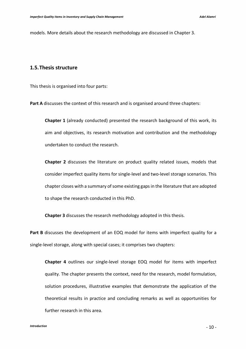
1.5. Thesis structure
This thesis is organised into four parts:
Part A discusses the context of this research and is organised around three chapters:
Chapter 1 (already conducted) presented the research background of this work, its
aim and objectives, its research motivation and contribution and the methodology
undertaken to conduct the research.
Chapter 2 discusses the literature on product quality related issues, models that
consider imperfect quality items for single-level and two-level storage scenarios. This
chapter closes with a summary of some existing gaps in the literature that are adopted
to shape the research conducted in this PhD.
Chapter 3 discusses the research methodology adopted in this thesis.
Part B discusses the development of an EOQ model for items with imperfect quality for a
single-level storage, along with special cases; it comprises two chapters:
Chapter 4 outlines our single-level storage EOQ model for items with imperfect
quality. The chapter presents the context, need for the research, model formulation,
solution procedures, illustrative examples that demonstrate the application of the
theoretical results in practice and concluding remarks as well as opportunities for
further research in this area.

imperfect Quality Items in Inventory and Supply Chain Management Adel Alamri
Introduction
- 11 -
Chapter 5 emphasises the versatile nature of the proposed model. In particular, we
derive a general step-by-step solution procedure for continuous intra-cycle periodic
review applications, account for an appropriate management of perishable
inventories, explore coordination mechanisms, link the model to some practical
situations for inventory management and provide a summary of implications and
managerial insights.
Part C presents EOQ models for a two-level storage and special cases. It consists of three
chapters:
Chapter 6 introduces our first two-level storage EOQ model for items with imperfect
quality that underlies a Last-In-First-Out (LIFO) dispatching policy. We present the
context, need for the research, model formulation, solution procedures, illustrative
examples that demonstrate the application of the theoretical results in practice and
concluding remarks, as well as opportunities for further research in this area.
Chapter 7 proposes our second two-level storage EOQ model for items with imperfect
quality that considers a First-In-First-Out (FIFO) dispatching policy. The chapter is
organised as above.
Chapter 8 suggests a new framework for a two-level storage EOQ model for items with
imperfect quality. A new dispatching policy entitled Allocation-In-Fraction-Out (AIFO)
is presented. This chapter also follows the structure adopted in Chapter 6.
Part D comprises one chapter that summarises the overall contributions presented in this PhD
and provides a discussion of avenues for further research.
imperfect Quality Items in Inventory and Supply Chain Management Adel Alamri
Introduction
- 12 -
Chapter 9 highlights the overall contribution and findings of this work and the next
steps of research.
A pictorial overview of the structure of the thesis is offered in Fig. 1.1.
Fig.1.1 Thesis structure.
1• General introduction
2• literature review
3• Research methodology
4• A general EOQ model for imperfect quality items
5• Special cases of the general EOQ model
6• A general EOQ model for imperfect quality items under
LIFO dispatching policy
7• A general EOQ model for imperfect quality items under
FIFO dispatching policy
8• General EOQ models for imperfect quality items under
LIFO, FIFO and AIFO dispatching policies
9• Summary of contributions and further research

imperfect Quality Items in Inventory and Supply Chain Management Adel Alamri
Literature review
- 13 -
2. Literature review
The academic literature related to inventory control for imperfect quality items is
multidisciplinary in nature and, for presentation purposes in this PhD thesis, is thematically
organised around four main streams of research: 1) inventory quality related issues; 2)
information sharing and inspection processes; 3) model formulations and related solution
techniques that consider imperfect quality items; and 4) lot size inventory models with two
levels of storage. The academic literature related to the first, third and fourth themes are
reviewed. For the second theme, some discussion on the Value of Information (VOI) and
learning effect is conducted to enable linkage with the inspection process. This provides the
necessary background to position our study in the current body of literature and elaborate
on its research contributions. This review will also summarise and highlight the research gaps
identified in the literature that led to the formulation of the general EOQ models stated in
the previous chapter.
2.1. Inventory quality issues
One implicit assumption embedded in the EOQ model is that stored items preserve their
physical characteristics indefinitely. This assumption may hold true for certain commodities.
However, in real-life settings, items are subject to “perishability”, “deterioration” and
“obsolescence” that affect the physical state/fitness and behaviour of an item while in storage
or as it moves through the supply chain (Goyal and Giri, 2001b; Bakker et al., 2012; Pahl and
Voß, 2014). Next, we present an overview of previous studies related to the quality issues
considered in this thesis.

imperfect Quality Items in Inventory and Supply Chain Management Adel Alamri
Literature review
- 14 -
2.1.1. Perishability and lifetime constraints
Nahmias (1975, 1977) introduced the fixed lifetime case and analysed the problem of a
random lifetime product managed under periodic review with stationary stochastic demand.
He assumed no fixed order cost and backlogged demand and orders perishing in the same
sequence that they enter stock (i.e. a FIFO dispatching policy). Padmanabhan and Vrat (1995)
investigated an inventory model for perishable items with stock dependent selling rate. Abad
(1996) presented pricing and lot-sizing models under conditions of perishability and partial
backordering. Giri and Chaudhuri (1998) studied deterministic inventory models of perishable
product with stock dependent demand rate.
Skouri and Papachristos (2002) investigated a continuous review inventory model for
deteriorating items and time-varying demand rate. They assumed linear replenishment cost
and partial time-varying backlogging. Abad (2003) studied an optimal pricing and lot sizing
problem considering perishability, finite production, partial backordering and lost sales.
Ketzenberg et al. (2012) extended the work of Nahmias (1977) and addressed the random
lifetime as a function of the product’s time and temperature history (TTH) in the supply chain.
They allowed for orders to perish out of sequence, to discard inventory that remains good for
sale and to sell inventory that may have already perished.
Amorim et al. (2013) presented a classification of models for perishable items that have
explicit characteristics related to their physical status (e.g. by spoilage, decay or depletion)
and/or changes in their value as perceived by the customer and/or a risk of future reduced
functionality according to specialist opinion. Pahl and Voß (2014) provided a comprehensive
literature review that addresses deterioration and lifetime constraints of items.
imperfect Quality Items in Inventory and Supply Chain Management Adel Alamri
Literature review
- 15 -
Ketzenberg et al. (2015) considered a case in which, unsatisfied demand having been lost,
products may arrive already perished and orders may not perish in sequence.
2.1.2. Deterioration
Ghare and Schrader (1963) were among the first authors to address inventory problems
considering deteriorating products. Covert and Philip (1973) formulated an EOQ model in
which the deterioration rate follows a two parameter Weibull distribution. Shah and Jaiswal
(1977) and Aggarwal (1978) developed inventory models with a constant rate of
deterioration. Dave and Patel (1981) formulated an inventory model for deteriorating items
with time proportional demand. Hollier and Mak (1983) developed an inventory
replenishment policy for deteriorating items. They assumed constant rate of deterioration
and exponentially negative decreasing demand rate. Roychowdhury and Chaudhuri (1983)
presented an order level inventory model for deteriorating items with finite rate of
replenishment. Sachan (1984) extended the model of Dave and Patel (1981) to allow for
shortages. Dave (1986a, 1986b) proposed an order level inventory model for constant rate of
deterioration. Baker and Urban (1988) investigated a deterministic inventory system allowing
for stock dependent demand rate.
Datta and Pal (1988) developed an order level inventory model with power demand pattern
for items with variable rate of deterioration. Bahari-Kashani (1989) extended the model of
Dave and Patel (1981) to allow for variable replenishment periods. Datta and Pal (1990)
presented a note on an inventory model with stock dependent demand. Pal et al. (1993) and
Giri et al. (1996) developed deterministic inventory models for deteriorating items with stock
dependent demand rate. Wee (1993) proposed an economic production lot size model for

imperfect Quality Items in Inventory and Supply Chain Management Adel Alamri
Literature review
- 16 -
deteriorating items with partial back ordering. Hill (1995) studied EOQ models for
deteriorating items with time varying demand. Chang and Dye (1999) studied an order level
inventory model for deteriorating items with time-varying demand rate and partial
backlogging. Mandal and Maiti (1999) developed an inventory model of damageable items
with variable replenishment and stock dependent demand rate.
Gupta and Aggarwal (2000) presented an EOQ model for deteriorating items allowing for
production rate to be dependent on a linear trend in demand. Abad (2001) presented pricing
and lot-sizing models allowing for a variable rate of deterioration and partial backlogging.
Chang and Dye (2001) proposed an inventory model for deteriorating items with partial
backlogging and permissible delay in payments. Goyal and Giri (2001a) conducted an
extensive review of papers addressing deteriorating items since the early 1990s. Goyal and
Giri (2001b) extended the model of Chang and Dey (1999) for deteriorating items with time
varying demand and partial backlogging. Wee and Law (2001) proposed a deterministic
inventory model for deteriorating items under time-value of money and price-dependent
demand. Wang (2002) investigated an inventory replenishment policy for deteriorating items
with shortages and partial backlogging. Wu (2002) developed an EOQ inventory model for
items considering Weibull distribution deterioration rate, time-varying demand and partial
backlogging.
Khanra and Chaudhuri (2003) re-established an order-level inventory model for deteriorating
items with time-dependent quadratic demand. Zhou et al. (2003) formulated a new variable
production scheduling strategy for deteriorating items with time-varying demand and partial
lost sale. Chu and Chung (2004) discussed the sensitivity of the inventory model with partial
backorders. Chu et al. (2004) presented a note on inventory model with a mixture of back

imperfect Quality Items in Inventory and Supply Chain Management Adel Alamri
Literature review
- 17 -
orders and lost sales. Sana et al. (2004) formulated a production inventory model for
deteriorating items with trended demand and shortages. Zhou et al. (2004) studied a finite
horizon lot-sizing inventory model with time-varying demand and waiting time dependent
partial backlogging. Giri et al. (2005) proposed an economic production lot size inventory
model with increasing demand and partial backlogging. Teng and Chang (2005) studied an
EPQ model for deteriorating items with price and stock dependent demand.
Manna and Chaudhuri (2006) developed an EOQ model with ramp type demand and time
dependent deterioration rate. In that model, the unit production cost is inversely
proportional to the demand rate. Ouyang et al. (2006) studied an inventory model for non-
instantaneous deteriorating items with permissible delay in payments. Pal et al. (2006)
suggested an inventory model for deteriorating items with demand rate being dependent on
the displayed stock level. Wu et al. (2006) studied an optimal replenishment policy for non-
instantaneous deteriorating items with stock-dependent demand and partial backlogging.
Teng et al. (2007) extended the work of Abad (2003) considering shortage and lost sales costs
into the objective function. Liao (2008) developed an EOQ model with non-instantaneous
receipt and exponentially deteriorating items under two-level trade credit. Chung (2009)
presented a complete proof on the solution procedure for non-instantaneous deteriorating
items with permissible delay in payment.
Skouri et al. (2009) studied inventory models with ramp type demand rate, partial backlogging
and Weibull deterioration rate. Ahmed et al. (2013) formulated inventory models with ramp-
type demand rate, partial backlogging and general deterioration rate. Sarkar and Sarkar
(2013) presented an inventory model with stock-dependent demand, partial backlogging and
time-varying deterioration rate. Sicilia et al. (2014) developed a deterministic inventory

imperfect Quality Items in Inventory and Supply Chain Management Adel Alamri
Literature review
- 18 -
model for deteriorating items with shortages and time-varying demand.
2.2. Information sharing and inspection process
There is a unanimous agreement among researchers and practitioners on the benefits of
information sharing that allows more timely material flow in a supply chain (Costantino et al.,
2013). In many situations, products entail inspection to ensure an appropriate service to the
customers (White and Cheong, 2012). In this section, we first address the importance of VOI
in supply chains, followed by some discussion that links the VOI and learning effect with the
inspection process associated with the formulation of EOQ inventory models.
2.2.1. Value of information (VOI)
Value of information (VOI) in supply chains has become increasingly important and may relate
to sharing data over and above demand and inventory information (Dong et al., 2014; Kahn
1987; Metters 1997). For example, modern technologies, such as radio-frequency
identification (RFID) systems, data loggers and time–temperature integrators and sensors, are
capable of recording, tracking and transmitting information regarding an item as it moves
through the supply chain (Jedermann et al., 2008). The deployment of such technologies
increases supply chain visibility, which in turn lowers safety stocks and improves customer
service level (Gaukler et al., 2007; Kim and Glock 2014).
Ketzenberg et al. (2007) conducted an extensive literature review of papers that: (1) address
VOI in the context of inventory control, (2) provide a numerical study to explore VOI over a
imperfect Quality Items in Inventory and Supply Chain Management Adel Alamri
Literature review
- 19 -
set of varying operating characteristics and (3) compare two or more scenarios. In addition,
they developed and tested a VOI framework to help identify the determinants of VOI. The
researchers pointed out that the dominant research stream in this area focuses on the value
of demand information to enhance supply chain performance.
Accurate shelf lifetime monitoring is a goal of technologies that have been developed to
collect and transmit data about the state of a product. For certain items, if temperature
departs from a pre-defined range, the items are spoiled and must be discarded (Zacharewicz
et al., 2011). Ketzenberg and Ferguson (2008) examined the VOI for a product with fixed
lifetime in the context of a serial supply chain. They evaluated the case in which a supplier
shares retailer demand and inventory information, as well as the case where a centralised
decision maker collects full information at both echelons. Recently, Ketzenberg et al. (2015)
addressed the VOI for inventory replenishment decisions to demonstrate the wide
fluctuations in a supply chain’s TTH, the applicability and accuracy of using RFID temperature
tags to capture the TTH, and the use of TTH to model shelf lifetime.
The focus of this PhD thesis is on the value and use of technologies, such as RFID, to capture
the TTH to model shelf lifetime and not the technologies themselves. For further details
related to this technology, see Jedermann et al. (2008) and Wessel (2007).
2.2.2. Learning effects
The ‘Learning Phenomenon’ introduced by Wright (1936) implies that the performance of a
system engaged in a repetitive task improves with time. The learning phenomenon is
reflected by the “learning curve” theory, which links the performance of a specific task with

imperfect Quality Items in Inventory and Supply Chain Management Adel Alamri
Literature review
- 20 -
the number of times that the task is repeated. Wright’s power function formulation (which
was based on empirical data) suggests that as production accumulates, the unit production
time decreases by a constant percentage (e.g. 80 per cent, 70 per cent, etc.) each time the
quantity doubles.
Wright’s simple mathematical formulation is a commonly used model because it is easier to
implement and understand by practitioners than those complex ones (e.g. Hackett, 1983;
Towill, 1982, 1985). However, it implies that production time can be neglected as the
cumulative quantity produced takes on relatively larger values. This is an unreasonable
conclusion, since in real-world problems, after a certain time of cumulative learning in a
production system, the system plateaus, in which case the production time will attain an
almost certain value.
Jordan (1965) and Carlson and Rowe (1976) argued that in practice, the learning function is
an “S”-shaped curve. The task “life cycle” depicted by an S-shaped logistic learning curve
comprises three phases. In the first phase (incipient), the worker is becoming acquainted with
the techniques, tools, procedures, work place, facilities, etc. In this phase improvement is
slow, which is consistent with the behaviour observed in many industrial situations. The
second phase (learning) is where most improvement occurs. The third phase (maturity)
denotes the levelling of the curve.
There is almost unanimous agreement among researchers and practitioners that the
preponderant form of a learning curve is either an S-shaped (Jordan, 1958; Carlson, 1973) or
a power one, as suggested by Wright (1936) (Alamri and Balkhi, 2007; Dar-El, 2000; Jaber,
2006). For more discussion on learning curves, interested reader may refer to Grosee et al.
(2015).

imperfect Quality Items in Inventory and Supply Chain Management Adel Alamri
Literature review
- 21 -
2.2.3. Inspection process
The above discussion raised in Sections 2.2.1 and 2.2.2 relates very much to knowledge
acquired from an inspection process conducted at the retailer site. This means that the quality
issues that render an item defective can be communicated to the supplier in order to reduce
the potential risks affecting such defectiveness. These risks can be attributed to production,
handling or transportation errors.
Although the buyer is often credited, so that no costs apply for defective items, the potential
interest remains to eliminate the presence of defects in subsequent replenishments.
Therefore, coordination may be pursued between supply chain members implying that any
information gained through previous replenishments can be used to enhance subsequent
deliveries.
White and Cheong (2012) considered the benefit of observing the quality of a perishable
product in a food supply chain that is processed in multiple stages from origin to destination.
At each stage, it is presumed essential to decide whether to inspect the quality of the product
at a certain cost. Moussawi-Haidar et al. (2013) investigated an instantaneous replenishment
model under the effect of a sampling policy for defective items.
Inspection may also be presumed essential for updating the Information System records with
good items that are actually available in stock, so as to avoid shortages. Moreover, inspection
may eliminate the return service cost associated with product recalls (Klassen and Vereecke
2012). It can be used in real-life settings where the impact of allowing through defective items
could be severe. Different types of inspection can occur, including seal inspection, outer case
label inspection or damaged carton inspection. The service cost may include goodwill cost,
transportation cost, and re-processing cost, and that may affect all supply chain members.

imperfect Quality Items in Inventory and Supply Chain Management Adel Alamri
Literature review
- 22 -
Inspection may also reduce holding costs due to the deployment of less preserving
environmental conditions, i.e. the defective items are not usually stored in the same
warehouse where the good items are stored (e.g. Wahab and Jaber, 2010).
2.3. Inventory models with imperfect quality items
The classical EOQ has been a widely-accepted model for inventory control purposes due to
its simple and intuitively appealing mathematical formulation. However, it is true to say that
the operation of the model is based on a number of explicitly or implicitly made, unrealistic,
mathematical assumptions that are never actually met in practice (Jaber et al., 2004; Liao et
al., 2013). For example, the assumption of perfect quality items is technologically
unattainable in most supply chain applications and it is an important restriction in the classical
formulation of the EOQ model (Cheng, 1991).
In a centralised scenario, there is a single decision-maker who is concerned with maximising
the entire chain's profit. The objective is to find a more profitable joint production and
inventory strategy, as compared to the strategy resulting from independent decision making.
In a decentralised, coordinated scenario, the supplier and the retailer cooperate in order to
render the total minimum (maximum) cost (revenue) closer to that associated with a
centralised one.
In this section, we present a review of previous studies related to the formulation of the EOQ
model with imperfect quality items. Section 2.3.1 will focus on papers that considered the
formulation of a single warehouse inventory model, followed by a review of studies
investigating the effect of learning on a single warehouse inventory model with imperfect

imperfect Quality Items in Inventory and Supply Chain Management Adel Alamri
Literature review
- 23 -
quality items in Section 2.3.2. Previous studies related to the formulation of a joint-vendor-
buyer inventory model with imperfect quality items are presented in Section 2.3.3.
2.3.1. Single-warehouse model
Porteus (1986) studied the impact of imperfect products when the production process may
shift randomly from an in-control state to an out-of-control state during a production run. He
assumed that all imperfect items could be reworked. Similarly, Rosenblatt and Lee (1986)
considered the effects of an imperfect manufacturing process on the determination of an
optimal manufacturing cycle time.
Salameh and Jaber (2000) developed a mathematical model that permits some of the items
to drop below the quality requirements, i.e. a random proportion of defective items is
assumed for each lot size shipment, with a known probability distribution. The researchers
assumed that each lot is subject to a 100 per cent screening, where defective items are kept
in the same warehouse until the end of the screening process and then can be sold at a price
lower than that of perfect quality items. Cárdenas-Barrón (2000) corrected a minor error
appearing on Salameh and Jaber’s model but did not diminish the main idea and the
contribution. Goyal and Cárdenas-Barrón (2002) developed a practical approach for
determining the economic production quantity. Chan et al. (2003) presented a similar model,
in which products are categorised as good quality, good quality after reworking, imperfect
quality, and scrap.
Chung and Huang, (2006) presented an inventory model which accounts for imperfect quality
items under the condition of permissible delay in payments. Papachristos and Konstantaras
imperfect Quality Items in Inventory and Supply Chain Management Adel Alamri
Literature review
- 24 -
(2006) investigated the sufficient condition proposed by Salameh and Jaber (2000) and Chan
et al. (2003), which is related to the issue of non-shortages. They pointed out that this
condition is not a sufficient condition to ensure that shortages will not occur. They also
extended the work of Salameh and Jaber in which imperfect items are removed by the end of
the cycle. Rezaei (2005), Eroglu and Ozdemir (2007) and Wee et al. (2007) extended the model
of Salameh and Jaber (2000) by allowing for shortages. Konstantaras et al. (2007) investigated
the case where imperfect quality items can be sold as a single batch at a lower price as well
as the case in which these items are reworked at a cost. Maddah and Jaber (2008) suggested
a new model that rectifies a flaw in the one presented by Salameh and Jaber (2000) using
renewal theory.
Jaggi and Mittal (2011) investigated the effect of deterioration on a retailer’s EOQ when the
items are of imperfect quality. In that paper, defective items were assumed to be kept in the
same warehouse until the end of the screening process. Jaggi et al. (2011) and Sana (2012)
presented inventory models, which account for imperfect quality items under the condition
of permissible delay in payments. Moussawi-Haidar et al. (2014) extended the work of Jaggi
and Mittal (2011) to allow for shortages.
2.3.2. Single-warehouse model with learning
Jaber et al. (2008) extended the work of Salameh and Jaber (2000) by considering that the
percentage of defective items per lot reduces according to a learning curve. They examined
empirical data from the automotive industry for several learning curve models and the S-
shaped logistic learning curve (Jordan, 1958; Carlson, 1973) was found to fit well.

imperfect Quality Items in Inventory and Supply Chain Management Adel Alamri
Literature review
- 25 -
Wahab and Jaber (2010) presented the case where different holding costs for good and
defective items are assumed. They showed that if the system is subject to learning, then the
lot size with the same assumed holding costs for the good and defective items is less than the
one with differing holding costs. When there is no learning in the system, the lot size with
differing holding costs increases with the percentage of defective items.
Konstantaras et al. (2012) pointed out that as learning in quality increases, then the lot size,
number of defective items and shortages decrease. Hlioui et al. (2015) investigated
replenishment, production and quality control strategies in a three-stage supply chain with
imperfect quality items. They pointed out that the integration of 100 per cent screening
process or discarding decisions is more beneficial, and assures better coordination at a lower
cost.
2.3.3. Vendor–buyer supply chain modelling
Zhang and Gerchak (1990) developed a joint lot sizing and inspection policy under an EOQ
model, in which a random proportion of the lot was considered defective. Wee (1995a)
presented a joint pricing and replenishment policy for deteriorating items with a declining
market. In a follow-up, Wee (1995b) developed a deterministic inventory model for
deteriorating items with shortages and a declining market. Yang and Wee (2002) investigated
the effect of deterioration and constant production and demand rates on a production
inventory policy with a single vendor and multiple buyers. Rau et al. (2003) proposed an
integrated inventory model for deteriorating items and derived an optimal joint total cost for
a multi-echelon supply chain environment.

imperfect Quality Items in Inventory and Supply Chain Management Adel Alamri
Literature review
- 26 -
Huang (2004) developed a model to determine an optimal integrated vendor–buyer inventory
policy for flawed items in a just-in-time manufacturing environment. Huang and Yao (2005)
studied an optimally coordinating inventory model for deteriorating items in a supply chain
system with a single vendor and multiple buyers. Lo et al. (2007) derived an integrated
vendor–buyer supply chain model with imperfect production processes. They assumed a
varying rate of deterioration, partial backordering and inflation. Sung and Gong (2008)
proposed a production inventory model for deteriorating production with defective items
being reworked and joint material replenishment policy being considered.
Singh and Diksha (2009) formulated an integrated vendor-buyer cooperative inventory model
for deteriorating items, allowing for multivariate demand and progressive credit period.
Wahab et al. (2011) developed an EOQ inventory model for a coordinated two-level supply
chain by allowing for shortages and environmental effects. Moussawi-Heidar and Jaber (2013)
proposed a joint model for cash and inventory management for a retailer under delay in
payments. Khan et al. (2014) presented an integrated vendor–buyer inventory policy by
accounting for learning in production at the vendors' end and quality inspection errors at the
buyers’ end.
Paul et al. (2014) presented a joint replenishment policy with imperfect quality items for
multiple products. Rad et al. (2014) derived an integrated vendor–buyer for a demand-driven
pricing model with imperfect production and shortages. Ongkunaruk et al. (2016) determined
the optimal reordering policy for multiple products in a joint replenishment problem. They
integrated shipment constraint, budget constraint and transportation capacity constraint. Yu
and Hsu (2017) derived a single-vendor, single-retailer, production-inventory model when a
100 per cent inspection is assumed with imperfect items being returned to vendor

imperfect Quality Items in Inventory and Supply Chain Management Adel Alamri
Literature review
- 27 -
immediately under an unequally sized shipment.
2.4. Two-warehouse model
The classical EOQ model is often based on the assumption that the OW has unlimited capacity.
However, there are many factors that may lead to purchasing a number of units that may
exceed the limited capacity of OW, resulting in the excessive units being stored in another
RW, which is assumed to be of ample capacity. Such factors may include a discounted price
of goods offered by the supplier, revenue (acquisition price) being higher than the holding
cost in RW, and evading high inflation rates.
The earliest approach to address the basic two-warehouse inventory model was recognised
by Hartley (1976). Sarma (1983) presented a deterministic two-warehouse inventory model
under an optimum release rule, in which the cost of transporting an item from RW to OW is
assumed. Murdeshwar and Sathe (1985) discussed some aspects of lot size model with two
levels of storage and derived the solution for optimum lot size under finite production rates.
Sarma (1987) considered a deterministic order level inventory model for deteriorating items.
He assumed a lower rate of deterioration in RW due to better preserving facilities. Goswami
and Chaudhuri (1992) developed a two-warehouse inventory model allowing for linear
demand and deterioration rates. Pakkala and Achary (1992) explored a deterministic two-
warehouse inventory model for deteriorating items with a finite replenishment rate assuming
uniform demand and shortages.
Bhunia and Maiti (1994) studied a two-warehouse inventory model for a single item with an
imperfect Quality Items in Inventory and Supply Chain Management Adel Alamri
Literature review
- 28 -
infinite rate of replenishment. They assumed a linear trend in demand and shortages were
allowed and fully backlogged. Ishii and Nose (1996) proposed a two-warehouse inventory
model for a perishable product with two types of customers, high priority and low priority
(the former buys only the newest commodity, while the latter buys either one). They assumed
that stock is depleted by high priority demand first and then low priority demand using FIFO
issuing policy; different selling prices reflecting the remaining lifetime of commodity are
assumed.
Roy and Maiti (1997) established a fuzzy EOQ model with two-level storage allowing for price
dependent demand. In that model, the setup cost varies with the quantity
produced/purchased. Bhunia and Maiti (1998a, 1998b) formulated a two-warehouse
inventory model for deteriorating items with linear trend in demand. Zhou (1998) and Lee
and Ma (2000) investigated a two-warehouse model for deteriorating items and time varying
demand. Kar et al. (2001) established a deterministic inventory model with two levels of
storage. They assumed linear time-dependent demand and finite time horizon. Zhou (2003)
considered a multi-warehouse inventory model for items with time-varying demand and
shortages.
Yang (2004) proposed a two-warehouse inventory problem for deteriorating items under
inflation. In that model, the inventory deteriorates at a constant rate and shortages were
allowed. Wee et al. (2005) investigated a two-warehouse inventory model with Weibull
distribution deterioration under inflation. They assumed partial backordering and applied the
discounted cash flow in problem analysis. Zhou and Yang (2005) presented a two-warehouse
model allowing for stock-level dependent demand rate.
Mandal et al. (2006) considered a two-warehouse inventory model for deteriorating items
imperfect Quality Items in Inventory and Supply Chain Management Adel Alamri
Literature review
- 29 -
with constant demand and deterioration rates. Yang (2006) extended his earlier model, Yang
(2004), accounting for partial backlogging and inflation. Dye et al. (2007) suggested a
deterministic two-warehouse inventory model for deteriorating items. They allowed for
shortages to occur in the OW with the backlogging demand rate being dependent on the
duration of the stock out.
Hsieh et al. (2008) formulated a deterministic two warehouses inventory model for
deteriorating items by minimising the net present value of the total cost. Rong et al. (2008)
investigated a two-warehouse inventory model for deteriorating items and shortages.
Thangam and Uthayakumar (2008) investigated a two-level supply chain model with partial
backordering and approximated Poisson demand. Lee and Hsu (2009) proposed a two-
warehouse production inventory model for deteriorating items and time-dependent
demands. Ghosh and Chakrabarty (2009) studied an order-level inventory model under two
levels of storage for deteriorating items and time-dependent demand. Jaggi et al. (2010)
proposed a two-warehouse inventory model for deteriorating items when demand is price
sensitive. Dem and Singh (2012) investigated a two-warehouse production model for
deteriorating items under quality consideration. Sett et al. (2012) developed a two-
warehouse production model assuming quadratically increasing demand and time-varying
deterioration. Agrawal et al. (2013) presented a two-warehouse inventory model with
constant deterioration rates, ramp-type demand and partial backlogging.

imperfect Quality Items in Inventory and Supply Chain Management Adel Alamri
Literature review
- 30 -
2.5. Summary
The effect of the presence of defective items on lot size has received the attention of many
researchers in the field. However, there has been little research that links the inspection
process with the management of perishable inventories. In parallel, it would be interesting to
explore the implications of the inspection process into inventory decision-making. Moreover,
a review of the literature reveals that there is no published work that derives solution
procedures for periodic review applications for the EOQ model with imperfect quality items.
The terms “deterioration”, “perishability” and “obsolescence” are used interchangeably in
the literature and may often be perceived as ambiguous because they are linked to specific
underlying assumptions regarding the physical state/fitness and behaviour of items over
time. In this thesis, we provide clearer definitions that distinguish the role of each term. For
example, deterioration indicates the process of decay, damage or spoilage of a product, i.e.
the product loses its value characteristics and can no longer be sold/used for its original
purpose. In contrast, an item with a fixed lifetime (expiration date) perishes once exceeding
its maximum shelf lifetime and thus it must be discarded. Obsolescence refers to items
incurring a partial or a total loss of value in such a way that the value for a product
continuously decreases with its perceived utility/desirability. Therefore, it would be value
adding to the literature of supply chain management if a detailed method is provided which
underpins and demonstrates how these terms may collectively apply to an item. It appears
also that the accuracy of continuous automated inventory control systems to model the shelf
lifetime of an item with imperfect quality is another research gap in this area.
The above identified research gaps are addressed in our first model that underlies an
imperfect Quality Items in Inventory and Supply Chain Management Adel Alamri
Literature review
- 31 -
inventory system with a single-level storage (OW). In particular, we present a general EOQ
model for items with imperfect quality under varying demand, defective items, a screening
process and deterioration rates for an infinite planning horizon. Consequently, the generality
of the model goes beyond academic interests to enable inventory managers to establish the
optimum order quantities that minimise the total system cost in different realistic situations.
It seems plausible to address the same identified research gaps when formulating an
inventory system with a two-level storage (OW and RW). However, this necessitates
formulation of LIFO and FIFO EOQ models for investigation and numerical comparison
purposes. As such, we propose and compare three general EOQ models with a two-level
storage considering different transportation costs associated with OW and RW. The first
model underlies LIFO, the second model underlies FIFO and the third model relates to our
new suggested dispatching policy, which implies simultaneous consumption fractions
associated with OW and RW and is entitled AIFO. In order to enhance this line of research,
we formulate a key performance indicator (KPI), i.e. an upper-bound (cost associated with
OW (RW) being idle) that renders AIFO the optimal dispatching policy.
The mathematical formulations consider arbitrary functions of time that allow the decision
maker to assess the consequences of a diverse range of strategies by employing a single
inventory formulation for each model. The proposed models may be viewed as realistic in
today’s competitive markets and reflective of several practical concerns with regard to
product quality related issues. These issues relate to imperfect items received from suppliers,
deterioration of goods during storage, potential dis-location of good and defective items,
tracking the quality of perishable products in a supply chain and transfer of knowledge from
one inventory cycle to another. We show that the solution to each underlying inventory
imperfect Quality Items in Inventory and Supply Chain Management Adel Alamri
Literature review
- 32 -
model, if it exists, is unique and global optimal.
In summary, the aim of this PhD thesis is to advance the current state of knowledge in the
field of inventory mathematical modelling and management by means of providing
theoretically valid and empirically viable generalised inventory frameworks to assist inventory
managers towards the determination of optimum order/production quantities that minimise
the total system cost. The obvious implications that can be derived from the general
formulations, along with the fact that many practical examples published in the literature for
generalised models in this area constitute special cases of our proposed models, make, we
feel, an important contribution to the supply chain literature.
imperfect Quality Items in Inventory and Supply Chain Management Adel Alamri
Research methodology
- 33 -
3. Research methodology
3.1. Introduction
Research paradigms may often be perceived as ambiguous, misleading or assumed,
frequently resulting in the terms “paradigm”, “methodology” and “method” being
considerably tangled and used interchangeably in the literature (McGregor and Murnane,
2010). Consequently, it is often difficult to recognise each paradigm that is linked to
particular, underlying assumptions about the reality, knowledge, values and logic of the
subject being investigated. Fortunately, recognition of the feasibility of each paradigm by its
philosophical underpinning in “methodologies” is key to reconciling the differences in
individual perceptions of the same social phenomenon, which in turn involves apprising the
methods and techniques adopted to shape research in this paradigm (McGregor, 2007; 2008).
Despite acknowledgment of these traditions as a means of shaping research, preference for
each tradition is based largely on its ability to answer the two fundamental questions
constituting epistemological and ontological orthodoxies. In the domain of ontology (the
nature of reality), scientists explore the form and nature of reality and, therefore, what can
be known about it. In the domain of epistemology (the nature of knowledge), scholars
investigate the nature of the relationship between the knower and what can be known (Guba
and Lincoln, 1994, p. 108). Hence, long-standing epistemological and ontological debate has
been centred on whether social reality and natural sciences can be conducted by using the
same ideologies (Bryman, 2015). In this context, positivism has emerged as a broad position
seeking to integrate deductive logic, precise empirical observations and individual behaviour
while aiming to explain numerous patterns of human activity.

imperfect Quality Items in Inventory and Supply Chain Management Adel Alamri
Research methodology
- 34 -
3.2. Epistemological and ontological orthodoxies
A survey of the literature reveals that “the rumours of positivism’s death within sociology
have been greatly exaggerated. Though it is not dead, positivism has become increasingly
encapsulated within the USA and disavowed in the UK, particularly in its ‘instrumental’ form”
(Gartrell and Gartrell, 2002, p.653). Positivism is generally known as an approach to the
methodology of science in which patterns and causal relations can be investigated and
disclosed through research. Moreover, and among a variety of definitions found in the
literature about positivism, one can deduce that a positivistic philosophical basis provides an
approach to investigate social reality by assuming that theory and observation are dependent
on each other and involve employing natural science methods and theories to explore current
observations, seeking regularities for the purpose of generalisation. With researchers
considering themselves isolated from the research setting and in an unbiased position of
observation, positivism can also be regarded as aiming to understand and predict reality,
where deterministic and reactive stances among people are assumed. Reality is assumed to
be objective, tangible, and fragmentable, with research findings being context independent
in order to provide a clear interpretation of separate objective and subjective data
(Mackenzie, 2011).
Given that positivism is the dominant epistemological position, researchers need to become
more conscious and seek appropriate materials to avoid the possible risk of misunderstanding
the nature of their own research. The presence of a few fundamentally misleading passages
found in many books and articles on positivism and the absence of unanimous agreement
among social scientists on a clear definition of the term “positivism”, could lead to rejection
for the wrong reasons (Persson, 2010).

imperfect Quality Items in Inventory and Supply Chain Management Adel Alamri
Research methodology
- 35 -
There is almost unanimous agreement among social scientists that a paradigm is a set of
values, concepts, assumptions and practices that collectively constitute a means by which
scientists perceive the world or reality under investigation and the effects of this knowledge
on research findings (McGregor and Murnane, 2010). It is worth noting that having an
appropriate paradigm is the basic platform a scientist uses for analysing research, which is
the true orientation of his or her control to infer unbiased perception of reality. This unbiased
perception, whether it relies on a recognised methodological approach, is appreciated as a
combination of multiple methods, or is a claim towards advancing the current state of
knowledge in either approaches, will remain insignificant unless it presents originality and/or
new insights that illuminate a specific line of research. Although positivism has been
described by many authors in pejorative terms (Mackenzie, 2011; Nairn, 2012), supply chain
research is known to be marginalised outside the positivist research paradigm.
Answering the above ontological question is a core characteristic that creates and tests
management theories. In other words, knowing what constitutes reality, and what the
consideration of a philosophy of science offers to supply chains, plays a significant role in how
to shape and form the subsequent knowledge generated (Burgess et al., 2006; Miller and
Tsang, 2010). Therefore, philosophies, worldviews and attitudes form the basis that enables
researchers to pose a research question, embrace a research strategy and employ
appropriate methods and reasoning approaches (Solem, 2003). In this regard, positivist
research paradigm comprises the empirical methodology where social reality is perceived as
being independent and data is derived from experimentation and observation, which in turn
can be measured and evaluated by rigorous scientific approaches (generating supportive
evidence) (Rohmann, 1999). Thus, scientific examinations are produced quantitatively in

imperfect Quality Items in Inventory and Supply Chain Management Adel Alamri
Research methodology
- 36 -
which the research findings must be repeatable to assure reliability as measures of research
quality; i.e. interested researchers can generate any future results employing the same
research methods. Moreover, these findings are governed by the cause-effect doctrines
aimed at defining stable patterns of social reality (Crotty, 1998; Marczyk et al., 2005; Neuman,
2002).
3.3. Research methods
Closely associated with the positivist paradigm is deductive mathematical modelling and its
associated scientific methods and techniques which are the most common quantitative ones
adopted in supply chain research (Sachan and Datta, 2005; Burgess et al., 2006; Spens and
Kovács, 2006; Aastrup and Halldórsson, 2008). Moreover, most research published in the top
Operational Research (OR) international journals primarily comprises theoretical
mathematical modelling, where research results are produced almost entirely within the
quantitative research domain (Lewis and Suchan, 2003; Sachan and Datta, 2005; Stock et al.,
2010).
Although researchers accept that supply chain management is more likely to be approached
quantitatively, this method has been subjected to criticism for not considering a more
inclusive, supply chain-wide system perspective and undermining the influence of social
structures and their relations to activity (Sachan and Datta, 2005). In this regard, recent calls
in top OR journals have invited scholars to consider more fully the importance of human
factors in supply chain management and to conduct behavioural studies.
Other examples of criticisms of the dominant supply chain management research paradigm
imperfect Quality Items in Inventory and Supply Chain Management Adel Alamri
Research methodology
- 37 -
from different philosophical domains includes, but not limited to, those raised by Faria and
Wensley (2002), Näslund (2002), Lewis and Suchan (2003) and New (2004). Within the long-
standing epistemological debate about the most appropriate philosophical position, other
researchers have claimed that the designability of supply chains adheres to a positivist
research paradigm with an inherent assumption that managers responsible for supply chain-
related activities and other related parties, such as being isolated from the context within
which they work and live, may act in predictable ways and accept designs as proposed without
questioning them (Aastrup and Halldórsson, 2008). This can be a valid criticism if, for example,
the reactions being experienced rely heavily on the managerial life experience of the subjects.
Instead, in well-established organisations, reactions are presumed to be dependent on the
implementation of either optimal and near optimal values derived or statistically projected
parameters.
Similarly, other works have focused primarily on the exclusion of elements such as context
and distribution of power and, consequently, call for the adoption of a new philosophy of
science perspectives that can discover reasons for the existence of phenomena, rather than
a perspective that can describe them and present solutions for reducing their effects (New
and Payne, 1995; Mangan et al., 2004; Spens and Kovács, 2005; Burgess et al., 2006; Boyer
and Swink, 2008; Stock et al., 2010; Tokar, 2010).
It is the very nature (not people related) of the majority of problems involved in OR that has
resulted in the dominance of quantitative methods. This is particularly true in statistical
inventory optimisation, whereby the scope of the problem (tremendous number of stock
keeping units involved) and the need for statistical optimisation calls for fully quantitative
approaches.

imperfect Quality Items in Inventory and Supply Chain Management Adel Alamri
Research methodology
- 38 -
3.4. Validity and reliability of the research
As discussed above, supply chain research has been characterised as being significantly
governed by a positivistic epistemological position that justifies the dominant ontological and
epistemological orthodoxies. In the domain of ontology, scholars agree that supply chains are
more likely to be perceived as inter-organisational entities that have ontological identities
generated independently of social bodies, relations and practices.
Despite the frequency and veracity of claims made regarding the ability of quantitative
methods to generate innovation, there is a natural dominance of quantitative, fully positivistic
approaches (Arlbjørn and Halldórsson, 2002; Näslund, 2002; Sachan and Datta, 2005). This is
because the intention is always to generalise and propose solutions that are sufficiently
robust to successfully apply in many different contexts. For example, in supply chain
mathematical modelling, the adoption of the positivistic paradigm is presumed essential for
facilitating the production of guidelines needed for optimised configurations and
improvement purposes, which, in most cases, are easy to implement among business entities.
Furthermore, the nature of this research is to formulate, solve and analyse mathematical
inventory models. Hence, the only ethical concerns to be considered when conducting
research is to accurately report both the methods and the results to allow interested readers
to derive, verify and compare research findings with currently available models.
Adamides et al. (2012) pointed out that the designability embedded in supply chains assumes
a flat ontology constructed on regularities at the activity level. In such a case, the constituting
activities of supply chains are being shaped according to the desired values of certain
performance levels. The potential question that arises here is how to attain validity and/or
imperfect Quality Items in Inventory and Supply Chain Management Adel Alamri
Research methodology
- 39 -
reliability without the presence of designability. For example, this designability is the
cornerstone for determining optimisation procedure required for the formulation, creation
and operationalisation of specific variables. These are collectively, under rigorous
mathematical assumptions, valid and reliable, particularly mathematical modelling
formulations and their associated science methods and techniques. Moreover, this
designability allows scholars to rectify any shortcomings that may appear in any mathematical
model and, thus, be able to refine the line of research. This is because researchers can
generate any future results produced by using the same research methods, whereby the
entire research process can be made value free to eliminate biased interpretations of the
results (Jantzen and Østergaard, 2001). Given that all research methodologies have their
weaknesses as well as their strengths, the methods and analytical tools employed by a
scholarly community may influence the very problems that do and do not receive the
attention of researchers (Martin, 1980).
3.5. Summary
So far, the motivation associated with relaxing some of the assumptions embedded in the
EOQ model for items with imperfect quality has been addressed. As the intended outcome is
presumed to be a theory-based research leading to widely applicable solutions, the positivist
epistemological framework will be embraced. It is often the case that a variety of practical
and complex inventory problems can be perceived as fully quantitative research studies. Thus,
a deductive approach is employed to incorporate non-linear programming techniques so as
to derive the solution procedure for the proposed models. It is, therefore, the aim of this
research to advance the current state of knowledge in the field of inventory mathematical

imperfect Quality Items in Inventory and Supply Chain Management Adel Alamri
Research methodology
- 40 -
modelling and management by means of providing theoretically valid and empirically viable
generalised inventory frameworks to assist inventory managers towards the determination
of optimum order/production quantities that minimise the total system cost.
To ascertain the validity of the research, and also for comparison purposes, all papers
contributing in the generalised work will be considered and the relevant models will be solved
to show that they constitute special cases of our proposed models.

imperfect Quality Items in Inventory and Supply Chain Management Adel Alamri
Part B
- 41 -
Part B: Lot size inventory model with one level of storage
This part consists of two chapters. Chapter 4 underlies a general EOQ model for imperfect
quality items and Chapter 5 covers special cases generated from the general model. In
Chapter 4, we present a general EOQ model for items that are subject to inspection for
imperfect quality. Each lot that is delivered to the sorting facility undergoes a 100 per cent
screening and the percentage of defective items per lot reduces according to a learning curve.
The generality of the model is viewed as important both from an academic and practitioner
perspective. The mathematical formulation considers arbitrary functions of time that allow
the decision maker to assess the consequences of a diverse range of strategies by employing
a single inventory model. A rigorous method is utilised to show that the solution is unique
and global optimal, and a general step-by-step solution procedure is presented for continuous
intra-cycle periodic review applications. The value of the temperature history and flow time
through the supply chain is also used to determine an appropriate policy. Furthermore,
coordination mechanisms that may affect the supplier and the retailer are explored to
improve inventory control at both echelons. In Chapter 5, we provide illustrative examples
and special cases that demonstrate application of the theoretical model in different settings
and lead to the generation of interesting managerial insights.
Part B is based on the paper entitled “Efficient inventory control for imperfect quality items”
by Adel Alamri, Irina Harris and Aris Syntetos, which has been published in the European
Journal of Operational Research (Alamri, et al. (2016)).

imperfect Quality Items in Inventory and Supply Chain Management Adel Alamri
A general EOQ model for imperfect quality items
- 42 -
4. A general EOQ model for imperfect quality items
4.1. Introduction
In this chapter, we present a general EOQ model for items with imperfect quality under
varying demand, defective items, a screening process and deterioration rates for an infinite
planning horizon. Consequently, the generality of the model extends beyond academic
interests to enable inventory managers to establish optimum order quantities that minimise
the total system cost. In the model, each lot is subject to a 100 per cent screening where items
that do not conform to certain quality standards are stored in a different warehouse.
Therefore, different holding costs for the good and defective items are considered in the
mathematical model.
Items deteriorate while they are in storage, with demand, screening and deterioration rates
being arbitrary functions of time. Thus, the decision maker can assess the consequences of a
diverse range of strategies by employing a single inventory model. The percentage of
defective items per lot reduces according to a learning curve. After a 100 per cent screening,
imperfect quality items may be sold at a discounted price as a single batch at the end of the
screening process or incur a disposal penalty charge.
A rigorous method is utilised to show that the solution, if it exists, is unique and global
optimal. Previously published models in this area are shown to be special cases of our model.
The behaviour of different conditions (such as using functions for varying demand, screening,
defectiveness and deterioration rates) is studied using illustrative examples, and interesting
insights are offered to practitioners.

imperfect Quality Items in Inventory and Supply Chain Management Adel Alamri
A general EOQ model for imperfect quality items
- 43 -
The remainder of the chapter is organised as follows: in Section 4.2 we emphasise the need
for the research. Our general EOQ model for items with imperfect quality, the assumptions
and notation of the inventory system are presented in Section 4.3. The solution procedures
are presented in Section 4.4, followed, in Section 4.5, by illustrative examples that
demonstrate the application of the theoretical results in practice. Managerial insights and
concluding remarks are provided in Section 4.6. The proof of the optimality and uniqueness
of our solution is presented in Appendix A.
4.2. Need for the research
The classical EOQ has been a widely accepted model for inventory control purposes due to its
simple and intuitively appealing mathematical formulation. However, the model is based on
a number of explicitly or implicitly made, unrealistic, mathematical assumptions that are
never actually met in practice (Jaber et al., 2004; Liao et al., 2013). Salameh and Jaber (2000)
presented a mathematical model in which a random proportion of defective items is assumed
for each lot size shipment. Maddah and Jaber (2008) developed a new model that rectifies a
flaw in the model presented by Salameh and Jaber (2000) using renewal theory. Jaber et al.
(2008) extended this by assuming the percentage of defective items per lot reduces according
to a learning curve. They examined empirical data from the automotive industry for several
learning curve models and the S-shaped logistic learning curve (Jordan, 1958; Carlson, 1973)
was found to fit well. Jaggi and Mittal (2011) investigated the effect of deterioration on a
retailer’s EOQ when the items are of imperfect quality.
In a real manufacturing environment, the defective items are not usually stored in the same

imperfect Quality Items in Inventory and Supply Chain Management Adel Alamri
A general EOQ model for imperfect quality items
- 44 -
warehouse as the good items. As a result, the holding cost must be different for the good
items and the defective ones (e.g. Paknejad et al., 2005). With this consideration in mind,
Wahab and Jaber (2010) presented the case where different holding costs for the good and
defective items are assumed. In this section, we have cited only references that are directly
relevant to this chapter. For more detail about the extension of a modified EOQ model for
imperfect quality items, see Khan et al. (2011).
One basic assumption of the above cited contributions is that the demand rate is assumed to
be constant and known. A survey of the inventory literature reveals that there is no published
work that investigates the model of Wahab and Jaber (2010) for time-varying demand and
product deterioration. Product life cycle analysis suggests that a constant demand rate
assumption is usually valid in the mature stage of the life cycle of the product. In the growth
and/or declining stages, the demand rate can be well approximated by a linear demand
function (e.g. Alamri and Balkhi (2007)). Also, one implicit assumption is that the stored items
that are screened may retain the same utility indefinitely, i.e. they do not lose their value as
time goes on. In fact, the variation of demand and/or product deterioration with time (or due
to any other factors) is a quite natural phenomenon.
4.3. Formulation of the general EOQ model
4.3.1. Assumptions and notation
The mathematical model is developed under the following assumptions and notation:
1. A single item is held in stock.
2. The lead-time is negligible, and no capacity restrictions are assumed, i.e. any

imperfect Quality Items in Inventory and Supply Chain Management Adel Alamri
A general EOQ model for imperfect quality items
- 45 -
replenishment ordered at the beginning of a cycle arrives just prior to the end of that
same cycle.
3. The demand, screening and deterioration rates are arbitrary functions of time
denoted by 𝐷(𝑡), 𝑥(𝑡)and𝛿(𝑡) respectively.
4. The percentage of defective items per lot reduces according to a learning curve
denoted by 𝑝d, where 𝑗 is the cycle index.
5. Shortages are not allowed, i.e. we require thate1 − 𝑝df𝑥(𝑡) ≥ 𝐷(𝑡)∀𝑡 ≥ 0.
6. The following notations are used for the cost parameters:
𝑐 is the unit purchasing cost.
𝑑 is the unit screening cost.
ℎ0 denotes the holding cost of good items per unit per unit time.
ℎi denotes the holding cost of defective items per unit per unit time.
𝑘 is the ordering cost per cycle.
4.3.2. The model
At the beginning of each cycle𝑗(𝑗 = 1, 2,… ), a lot of size 𝑄d is delivered, which covers the
actual demand and deterioration during both the first phase (screening) and the second
phase (non-screening). Each lot is subjected to a 100 per cent screening process at a rate of
𝑥(𝑡) that starts at the beginning of the cycle and ceases by time 𝑇jd, by which point in time
𝑄d units have been screened and 𝑦d units have been depleted, which is the summation of
demand and deterioration. During this phase, items not conforming to certain quality

imperfect Quality Items in Inventory and Supply Chain Management Adel Alamri
A general EOQ model for imperfect quality items
- 46 -
standards are stored in a different warehouse.
The variation in the inventory level during the first and second phases (Fig. 4.1) and the
variation in the inventory level for the defective items (shaded area) are given by (4.1), (4.3)
and (4.4) respectively.
iklm(1)i1
= −𝐷(𝑡) − 𝑝d𝑥(𝑡) − 𝛿(𝑡)𝐼0d(𝑡), 0 ≤ 𝑡 < 𝑇jd (4.1)
with the boundary condition 𝐼0d(0) = 𝑄d,
where
𝑄d = ∫ 𝑥(𝑢)𝑑𝑢opmq . (4.2)
iklm(1)i1
= −𝐷(𝑡) − 𝛿(𝑡)𝐼0d(𝑡), 𝑇jd ≤ 𝑡 ≤ 𝑇rd (4.3)
with the boundary condition 𝐼0de𝑇rdf = 0.
iksm(1)i1
= 𝑝d𝑥(𝑡), 0 ≤ 𝑡 ≤ 𝑇jd (4.4)
with the boundary condition 𝐼id(0) = 0.

imperfect Quality Items in Inventory and Supply Chain Management Adel Alamri
A general EOQ model for imperfect quality items
- 47 -
𝑄d 𝑄de1− 𝑝df − 𝑦d
𝑝d𝑄d 0 𝑇jd 𝑇rd Time Cycle length
Fig. 4.1. Inventory variation of an Economic Order Quantity (EOQ) model for one cycle.
The solutions of the above differential equations are:
𝐼0d(𝑡) = 𝑒/e0(1)/0(q)f ∫ 𝑥(𝑢)𝑑𝑢opmq − 𝑒/0(1) ∫ t𝐷(𝑢) + 𝑝d𝑥(𝑢)u𝑒0(v)𝑑𝑢
1q , 0 ≤ 𝑡 < 𝑇jd (4.5)
𝐼0d(𝑡) = 𝑒/0(1) ∫ 𝐷(𝑢)𝑒0(v)𝑑𝑢owm1 , 𝑇jd ≤ 𝑡 ≤ 𝑇rd (4.6)
𝐼id(𝑡) = ∫ 𝑝d𝑥(𝑢)𝑑𝑢1q , 0 ≤ 𝑡 ≤ 𝑇jd (4.7)
respectively, where
𝑔(𝑡) = ∫ 𝛿(𝑡) 𝑑𝑡. (4.8)
The per cycle cost components for the given inventory system are as follows:
Purchasing cost = 𝑐 ∫ 𝑥(𝑢)𝑑𝑢opmq . Note that this cost includes the defective and deteriorated
items.
Holding cost = ℎ0t𝐼0de0, 𝑇jdf + 𝐼0d(𝑇jd, 𝑇rd)u + ℎi𝐼ide0,𝑇jdf.
Inve
ntor
y le
vel

imperfect Quality Items in Inventory and Supply Chain Management Adel Alamri
A general EOQ model for imperfect quality items
- 48 -
Thus, the total cost per unit time of the underlying inventory system during the cycle t0, 𝑇rdu,
as a function of 𝑇jdand𝑇rd, say 𝑍(𝑇jd, 𝑇rd) is given by:
𝑍e𝑇jd, 𝑇rdf =jowmy(𝑐 + 𝑑) ∫ 𝑥(𝑢)𝑑𝑢 + ℎ0 z−𝐺(0)𝑒0(q) ∫ 𝑥(𝑢)𝑑𝑢opm
q +opmq
∫ 𝐷(𝑢)𝐺(𝑢)𝑒0(v)𝑑𝑢opmq + ∫ 𝑝d𝑥(𝑢)𝐺(𝑢)𝑒0(v)𝑑𝑢
opmq + ∫ 𝐷(𝑢)𝐺(𝑢)𝑒0(v)𝑑𝑢owm
opm{ +
ℎi z∫ t𝑇jd − 𝑢u𝑝d𝑥(𝑢)𝑑𝑢opmq { + 𝑘|, (4.9)
where
𝐺(𝑡) = ∫ 𝑒/0(1) 𝑑𝑡. (4.10)
Our objective is to find 𝑇jdand𝑇rd that minimise 𝑍(𝑇jd, 𝑇rd). However, the variables
𝑇jdand𝑇rd are related to each other as follows:
0 < 𝑇jd < 𝑇rd, (4.11)
𝑒0(q) ∫ 𝑥(𝑢)𝑑𝑢opmq = ∫ 𝐷(𝑢)𝑒0(v)𝑑𝑢owm
q + ∫ 𝑝d𝑥(𝑢)𝑒0(v)𝑑𝑢opmq . (4.12)
Thus, our goal is to solve the following optimisation problem, which we shall call problem(𝑚)
(𝑚) = }minimise𝑍e𝑇jd, 𝑇rdfgivenby(4.9)
subjectto(4.11)andℎd = 0�,
where
ℎd = 𝑒0(q) ∫ 𝑥(𝑢)𝑑𝑢opmq − ∫ 𝑝d𝑥(𝑢)𝑒0(v)𝑑𝑢
opmq − ∫ 𝐷(𝑢)𝑒0(v)𝑑𝑢owm
q .
It can be noted from Eq. (4.12), that 𝑇jd = 0 ⟹ 𝑇rd = 0 and 𝑇jd > 0 ⟹ 𝑇jd < 𝑇rd. Thus Eq.
(4.12) implies constraint (4.11). Consequently, if we temporarily ignore the monotony
imperfect Quality Items in Inventory and Supply Chain Management Adel Alamri
A general EOQ model for imperfect quality items
- 49 -
constraint (4.11) and call the resulting problem (𝑚j) then (4.11) does satisfy any solution of
(𝑚j). Hence (𝑚) and (𝑚j) are equivalent. Moreover, 𝑇jd > 0 ⟹ right-hand side (RHS) of
(4.6) > 0, i.e. Eq. (4.12) guarantees that the number of good items is at least equal to the
demand during the first phase.
4.4. Solution procedures
First, we note from (4.2) that 𝑇jd can be determined as a function of 𝑄d, say
𝑇jd = 𝑓jd(𝑄d). (4.13)
Taking also into account Eq. (4.12) we find that 𝑇rd can be determined as a function of 𝑇jd,
and thus of 𝑄d, say
𝑇rd = 𝑓rd(𝑄d). (4.14)
Thus, if we substitute (4.12)-(4.14) in (4.9) then problem (𝑚) will be converted to the
following unconstrained problem with the variable 𝑄d (which we shall call problem (𝑚r)).
𝑊e𝑄df =j�wmy(𝑐 + 𝑑) ∫ 𝑥(𝑢)𝑑𝑢 + ℎ0 z−𝐺(0)𝑒0(q) ∫ 𝑥(𝑢)𝑑𝑢�pm
q +�pmq
∫ 𝑝d𝑥(𝑢)𝐺(𝑢)𝑒0(v)𝑑𝑢�pmq + ∫ 𝐷(𝑢)𝐺(𝑢)𝑒0(v)𝑑𝑢�wm
q { + ℎi z∫ t𝑓jd − 𝑢u𝑝d𝑥(𝑢)𝑑𝑢�pmq { + 𝑘|.
(4.15)
Now, the necessary condition for having a minimum for problem (𝑚r) is
i�i�m
= 0. (4.16)
imperfect Quality Items in Inventory and Supply Chain Management Adel Alamri
A general EOQ model for imperfect quality items
- 50 -
To find the solution of (4.16), let 𝑊 = ��wm
then
i�i�m
=��m� �wm/�wm,�m
� �
�wmw , (4.17)
where 𝑤�m� and 𝑓rd,�m
� are the derivatives of 𝑤 and 𝑓rd with respect to (w.r.t) 𝑄d, respectively.
Hence, (4.16) is equivalent to
𝑤�m� 𝑓rd = 𝑓rd,�m
� 𝑤. (4.18)
Also, taking the first derivative of both sides of (4.12) (w.r.t) 𝑄d we obtain
𝑒0(q) − 𝑝d𝑒0(�pm) = 𝑓rd,�m� 𝐷e𝑓rdf𝑒0e�wmf. (4.19)
From which and (4.13)-(4.15) we have
𝑤�m� = (𝑐 + 𝑑) + ℎ0 zA𝐺e𝑓rdf − 𝐺(0)G 𝑒0(q) + A𝐺e𝑓jdf − 𝐺e𝑓rdfG 𝑝d𝑒0e�pmf{ +
�s�e�pmf
∫ 𝑝d𝑥(𝑢)𝑑𝑢�pmq . (4.20)
Also, (4.18) ⇔ 𝑊 = ��wm
=��m�
�wm,�m� , (4.21)
where 𝑊 is given by (4.15) and 𝑤�m�
is given by (4.20). Eq. (4.21) can be used to determine the
optimal value of 𝑄d and its corresponding total minimum cost. Then the optimal values of
𝑇jdand𝑇rd can be found from (4.13) and (4.14), respectively.

imperfect Quality Items in Inventory and Supply Chain Management Adel Alamri
A general EOQ model for imperfect quality items
- 51 -
4.5. Illustrative examples for different settings
In this section, we present examples to illustrate the theoretical application of our
mathematical model and solution procedure, whereby we consider scenarios with varying
demand, screening, defectiveness and deterioration rates.
4.5.1. Varying demand, screening, defectiveness and deterioration rates
In practice, the demand for products relies heavily on price (when price elasticity holds), time
and quality (Karmarkar and Pitbladdo, 1997). In addition, increasing (decreasing) demand
functions over time with quadratic, linear, exponential and stock-dependent trends is a
natural phenomenon (Murdeshwar, 1988; Hariga and Benkherouf, 1994; Datta et al. 1998;
Alamri, 2011; Benkherouf et al., 2014 ). For example, essential commodities and seasonal
products may follow steadily increasing quadratic or linear demand functions over time
(Mandal and Maiti, 2000). On the other hand, exponentially increasing demand applies to
products such as new spare parts, new electronic chips and seasonal goods in which the
demand rate is likely to increase very rapidly with time (Sana, 2010). Moreover, in some
countries (e.g. Saudi Arabia), the entire national (private and government) economy is
influenced by such phenomenon. For example, during the month of Ramadan, demand rate
for certain commodities and services is likely to increase very fast with time. This can be
justified by the fact that the number of visitors increases with time and the fact that
customers consumption behaviour during this month differs form that during other months.
However, before the end of this month, demand rate for such commodities is likely to
decrease very fast with time. Such phenomenon appears also in Saudi Arabia during the
imperfect Quality Items in Inventory and Supply Chain Management Adel Alamri
A general EOQ model for imperfect quality items
- 52 -
period of Hajj, i.e. the period in which the world's biggest annual gathering of people takes
place. In such period, demand rate for certain commodities and services is likely to increase
very fast with time until a specific point in time and then demand rate is likely to decrease
very fast with time. As such, the mathematical formulation presented in this PhD thesis
considers arbitrary functions of time, i.e. the mathematical formulation has no restriction on
all functions modelled. This implies that many functions can be incorporated to allow the
decision maker to assess and compare the consequences of a diverse range of strategies by
employing a single inventory model.
It is worth noting that the dominant form of a learning curve implemented by researchers
and practitioners alike is either an S-shaped (Jordan, 1958; Carlson, 1973), or a power one as
suggested by Wright (1936); please refer to Jaber (2006) for discussion on this issue.
In this example (Example 4.1), we consider the following functions for varying demand,
screening, defectiveness, and deterioration rates:
𝑥(𝑡) = 𝑎𝑡 + 𝑏,𝐷(𝑡) = 𝛼𝑡 + 𝑟,
𝑝d =𝜏
𝜋 + 𝑒¢d ,𝛿(𝑡) =𝑙
𝑧 − 𝛽𝑡
where 𝑏, 𝑟, 𝜋, 𝑧 > 0; 𝑎, 𝛼, 𝛾, 𝑙, 𝜏, 𝛽, 𝑡 ≥ 0,and𝛽𝑡 < 𝑧.
The parameter "𝛼” represents the rate of change in the demand. The case of 𝛼 = 0 reflects
a constant demand rate, when then 𝐷(𝑡) = 𝑟∀𝑡 ≥ 0. A similar behaviour is observed for the
effect of "𝑎”, the rate of change in the screening rate. Note that 𝛿(𝑡) is an increasing function
of time. The case of 𝛽 = 0 reflects a constant deterioration rate and 𝑙 = 0 corresponds to the
case associated with no deterioration. The percentage of defective items per lot reduces

imperfect Quality Items in Inventory and Supply Chain Management Adel Alamri
A general EOQ model for imperfect quality items
- 53 -
according to an S-shaped logistic learning curve (Jordan, 1958; Carlson, 1973), where𝜏 and𝜋
are model parameters, 𝛾 is the learning exponent and 𝑗 is the cycle index. The case 𝛾 = 0
applies to a constant percentage of defective items per lot.
The problem (𝑚r) has been coded in MATLAB for the above demand, screening,
defectiveness and deterioration rates and solutions were obtained using Eq. (4.21) for a wide
range of the control parameter values. Here, we adopt the values considered in the study by
Wahab and Jaber (2010), that are presented in Table 4.1 below.
Table 4.1. Input parameters for Example 4.1.
ℎ0 ℎi 𝑐 𝑑 𝑎 𝑏
20 5 100 0.50 1000 100200
Dollars/unit/year Dollars/unit/year Dollars/unit Dollars/unit Units/year Units/year
𝛼 𝑟 𝑙 𝑧 𝛽 𝑘
500 50000 1 20 25 3000
Units/year Units/year Units/year Units/year Units/year Dollars/cycle
𝜏 𝜋 𝛾
70.067 819.76 0.7932
Units/year Units/year Units/year
The optimal values of 𝑄d∗, 𝑇jd∗ , 𝑇rd∗ , 𝜔d∗, and the corresponding total minimum cost for 10
successive cycles are obtained and the results are shown in Table 4.2. In the first cycle, we
have taken 𝑝j = 0.08524resulting in a total number of 𝑄j∗ = 3550units, which is screened
by time 𝑇jj∗ = 0.0354 ≅ 13days and consumed by time 𝑇rj∗ = 0.0648 ≅ 24days. The total
minimum cost per year is 𝑊j∗ = 5585464dollars and the total minimum cost per cycle is
𝑤j∗ = 362030dollars. The number of defective items is 𝑝j𝑄j∗ = 303 units and the number
of deteriorated items is 𝜔j∗ = 5.4units, which is the difference between the actual demand
and the amount held in stock at the beginning of the cycle, excluding the number of defective
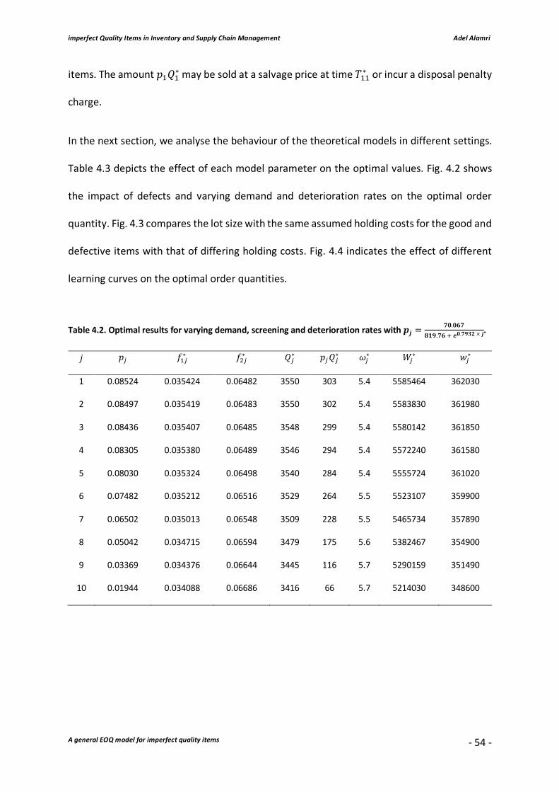
imperfect Quality Items in Inventory and Supply Chain Management Adel Alamri
A general EOQ model for imperfect quality items
- 54 -
items. The amount 𝑝j𝑄j∗ may be sold at a salvage price at time 𝑇jj∗ or incur a disposal penalty
charge.
In the next section, we analyse the behaviour of the theoretical models in different settings.
Table 4.3 depicts the effect of each model parameter on the optimal values. Fig. 4.2 shows
the impact of defects and varying demand and deterioration rates on the optimal order
quantity. Fig. 4.3 compares the lot size with the same assumed holding costs for the good and
defective items with that of differing holding costs. Fig. 4.4 indicates the effect of different
learning curves on the optimal order quantities.
Table 4.2. Optimal results for varying demand, screening and deterioration rates with 𝒑𝒋 =𝟕𝟎.𝟎𝟔𝟕
𝟖𝟏𝟗.𝟕𝟔¸𝒆𝟎.𝟕𝟗𝟑𝟐×𝒋.
𝑗 𝑝d 𝑓jd∗ 𝑓rd∗ 𝑄d∗ 𝑝d𝑄d∗ 𝜔d∗ 𝑊d∗ 𝑤d∗
1 0.08524 0.035424 0.06482 3550 303 5.4 5585464 362030
2 0.08497 0.035419 0.06483 3550 302 5.4 5583830 361980
3 0.08436 0.035407 0.06485 3548 299 5.4 5580142 361850
4 0.08305 0.035380 0.06489 3546 294 5.4 5572240 361580
5 0.08030 0.035324 0.06498 3540 284 5.4 5555724 361020
6 0.07482 0.035212 0.06516 3529 264 5.5 5523107 359900
7 0.06502 0.035013 0.06548 3509 228 5.5 5465734 357890
8 0.05042 0.034715 0.06594 3479 175 5.6 5382467 354900
9 0.03369 0.034376 0.06644 3445 116 5.7 5290159 351490
10 0.01944 0.034088 0.06686 3416 66 5.7 5214030 348600

imperfect Quality Items in Inventory and Supply Chain Management Adel Alamri
A general EOQ model for imperfect quality items
- 55 -
4.5.2. Sensitivity analysis
The results presented in Table 4.3 summarise the sensitivity analysis of the optimal order
quantity, total minimum cost per unit time and total minimum cost per cycle with respect to
all model parameters. The first row represents the original values of the proposed model and
the last one yields the values of the EOQ model. Fig. 4.2 depicts the effect of each additional
model parameter on the EOQ, i.e. the first three values represent the lot sizes of the last three
rows (EOQ, EOQ with defect and EOQ with the dis-location of good and defective items,
respectively). Whereas the following values reflect the effect of each additional model
parameter on the EOQ (Fig. 4.2). Fig. 4.3 replicates the first two rows of Table 4.3 for 10
consecutive cycles to compare the case of having the same holding costs for the good and
defective items with that of differing holding costs. Example 4.1 is replicated for 20
consecutive cycles to compare 𝑝d =½
¾¸¿Àm (Jordan, 1958; Carlson, 1973) with 𝑝d =
½¾¸j
𝑗/¢
(Wright, 1936) and the result is shown in Fig. 4.4 for 𝜏 = 40, 𝜋 = 999, 𝛾 = 0.75.

imperfect Quality Items in Inventory and Supply Chain Management Adel Alamri
A general EOQ model for imperfect quality items
- 56 -
Table 4.3. Sensitivity analysis for the general model.
𝑎 𝑏 𝛼 𝑟 𝑝d ℎ0 ℎi 𝑙 𝑧 𝛽 𝑓rd∗ 𝑄d∗ 𝜔d∗ 𝑊d∗ 𝑤d∗
1000 100200 500 50000 0.08524 20 5 1 20 25 0.06482 3550 5.4 5585464 362030
1000 100200 500 50000 0.08524 20 20 1 20 25 0.06397 3504 5.2 5586696 357370
1000 100200 500 50000 0.08524 20 5 1 40 25 0.06874 3762 3 5580407 383600
1000 100200 500 50000 0.08524 20 5 1 10 25 0.05827 3196 9 5595130 326040
1000 100200 500 50000 0.08524 20 5 1 20 50 0.06440 3528 5.5 5585745 359730
1000 100200 500 50000 0.08524 20 5 1 20 10 0.06505 3563 5.4 5585305 363310
1000 100200 500 50000 0.08524 20 5 1 20 0 0.06519 3571 5.6 5585202 364110
0 100200 500 50000 0.08524 20 5 1 20 25 0.06482 3550 5.4 5585464 362030
-1000 100200 500 50000 0.08524 20 5 1 20 25 0.06482 3550 5.4 5585464 362030
1000 100200 0 50000 0.08524 20 5 1 20 25 0.06612 3621 5.6 5583646 369190
1000 100200 -500 50000 0.08524 20 5 1 20 25 0.06751 3695 5.9 5581790 376800
0 100200 0 50000 0.08524 20 5 1 20 25 0.06612 3621 5.6 5583646 369190
0 100200 500 50000 0.08524 20 5 0 20 25 0.07321 4003 0 5575183 408140
0 100200 0 50000 0.08524 20 5 0 20 25 0.07511 4105* 0 5573127 418590
0 100200 0 50000 0.08524 20 20 0 20 25 0.07380 4034* 0 5574546 411390
0 100200 0 50000 0 20 20 0 20 25 0.07746 3873 0 5102460 395230
* The order quantity as in Wahab and Jaber (2010).
Fig. 4.2. The effect of each additional model parameter on the Economic Order Quantity (EOQ).
EOQ p hd a A l/z B3500
3600
3700
3800
3900
4000
4100
4200
Model parameters
Q*
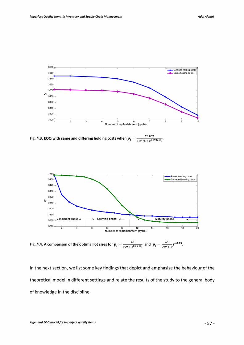
imperfect Quality Items in Inventory and Supply Chain Management Adel Alamri
A general EOQ model for imperfect quality items
- 57 -
Fig. 4.3. EOQ with same and differing holding costs when 𝒑𝒋 =𝟕𝟎.𝟎𝟔𝟕
𝟖𝟏𝟗.𝟕𝟔¸𝒆𝟎.𝟕𝟗𝟑𝟐×𝒋.
Fig. 4.4. A comparison of the optimal lot sizes for 𝒑𝒋 =𝟒𝟎
𝟗𝟗𝟗¸𝒆𝟎.𝟕𝟓×𝒋 and 𝒑𝒋 =
𝟒𝟎𝟗𝟗𝟗¸𝟏
𝒋/𝟎.𝟕𝟓.
In the next section, we list some key findings that depict and emphasise the behaviour of the
theoretical model in different settings and relate the results of the study to the general body
of knowledge in the discipline.
1 2 3 4 5 6 7 8 9 103400
3420
3440
3460
3480
3500
3520
3540
3560
3580
Number of replenishment (cycle)
Q*
Differing holding costsSame holding costs
2 4 6 8 10 12 14 16 18 203370
3380
3390
3400
3410
3420
3430
3440
3450
3460
Number of replenishment (cycle)
Q*
Power learning curve S-shaped learning curve
Incipient phase Learning phase Maturity phase

imperfect Quality Items in Inventory and Supply Chain Management Adel Alamri
A general EOQ model for imperfect quality items
- 58 -
4.5.3. Findings
• Table 4.2 indicates that the total minimum cost per year and the total minimum cost
per cycle decrease as learning increases, which supports the findings presented by
Jaber et al. (2008) and Wahab and Jaber (2010).
• The tabulated results indicate that all optimal quantities decrease as learning
increases, except for the amount of deteriorated items that incur a minor increase
that can be justified by the slight increase in the cycle length (Table 4.2).
• The presence of defects and varying demand and deterioration rates significantly
impact on the optimal order quantity (Table 4.2 and Fig. 4.2).
• The lot size with the same assumed holding costs for the good and defective items is
less than the one with differing holding costs. However, the difference between the
two quantities vanishes as 𝑝d takes on relatively small values (Fig. 4.3). Such finding is
consistence with that presented by Jaber et al. (2008).
• The results in Table 4.2 show a slight decrease in the total minimum cost per year due
to a slight decrease in 𝑝d. This is true in the incipient phase when an S-shaped logistic
learning curve is assumed, which is consistent with the behaviour of slow
improvement observed in this short phase, making the S-shaped learning curve an
appropriate model to use (Dar-El, 2000). On the other hand, this is not the case when
Wright’s learning curve is considered, which then leads to smaller quantities in the
incipient phase and hence the total minimum cost per year behaves similarly (Fig. 4.4).
Fig. 4.4 indicates that the reduction in the total minimum cost per year and the
optimal order quantities follow the same fashion as that of 𝑝d.
• The effect of 𝛼, the rate of change in the demand significantly influences the optimal
order quantity and the total minimum cost per year (Table 4.3). Moreover, this effect

imperfect Quality Items in Inventory and Supply Chain Management Adel Alamri
A general EOQ model for imperfect quality items
- 59 -
holds true for the case in which the deterioration rate is assumed to be of a fixed value
as well as for the case associated with no deterioration (Table 4.3).
• The presence of deterioration has a significant impact on the optimal order quantity
and the total minimum cost per year (Table 4.3). Such finding is consistence with that
presented by Moussawi-Haidar et al. (2014).
• A comparison between the results obtained in Tables 4.2 and 4.3 reveals that the
reduction of the optimal order quantity does not imply that the total minimum cost
per year decreases; in fact, it may increase.
• Previously published models in this area are shown to be special cases of our model
(Table 4.3).
4.6. Conclusion and further research
In this section, we summarise and emphasise the financial implications and managerial
aspects of our work to illustrate the theoretical application of our mathematical model.
In this chapter, a general EOQ model for items with imperfect quality was presented. The
general model developed in this chapter reflects a number of practical concerns with regard
to product quality related issues and may assist operations managers to respond to many
real-world challenges/opportunities for inventory improvements. Those opportunities
include poor supplier service levels (imperfect items received from suppliers), potential dis-
location of good and defective items (different warehouses for the good and defective items),
and transfer of knowledge from one inventory cycle to another.
Each lot is subjected to a 100 per cent screening and the percentage of defective items per

imperfect Quality Items in Inventory and Supply Chain Management Adel Alamri
A general EOQ model for imperfect quality items
- 60 -
lot reduces according to a learning curve. Items not conforming to certain quality standards
are stored in a separate facility with different holding costs for the good and defective items
being considered.
We presented illustrative examples to support application of the model and solution
procedure in different realistic situations. The obtained numerical results reflect the learning
effects incorporated in the proposed model. The presence of product deterioration and
varying demand rate significantly impact on the optimal order quantity. We observed the
effect of changing all model parameters and found that a reduction in the optimal order size
does not necessarily lead to a lower total minimum cost per unit time.
The generality of our model stems from the fact that the demand, screening, and product
deterioration rates are arbitrary functions of time. The proposed model unifies and extends
the academic literature related to imperfect quality items, which is quite diverse in nature.
Practical examples that are published in the literature for generalised models are used to
demonstrate that the solution is the same as in published sources, i.e. the validity of the
general model is ascertained. The versatile nature of our model and the fact that it may
accommodate many real-world concerns has been emphasised, whereby the results obtained
are compatible with the behaviour observed in many real-life settings. A mathematical proof
was presented (Appendix A), which shows that the solution to the underlying inventory
model, if it exists, is unique and global optimal. To the best of our knowledge, this appears to
be the first time that such a general EOQ model is formulated, investigated, and numerically
verified.
Based on the findings of this chapter, several interesting lines of further inquiry can be
addressed for finite or infinite planning horizons; for example:
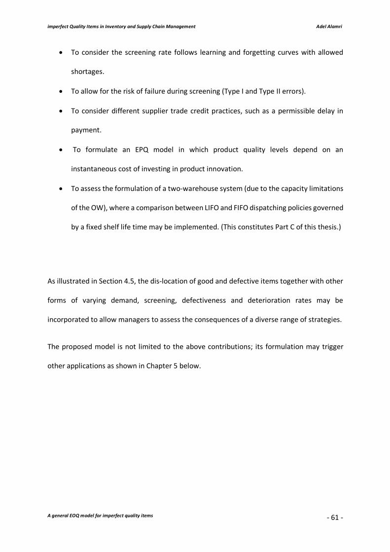
imperfect Quality Items in Inventory and Supply Chain Management Adel Alamri
A general EOQ model for imperfect quality items
- 61 -
• To consider the screening rate follows learning and forgetting curves with allowed
shortages.
• To allow for the risk of failure during screening (Type I and Type II errors).
• To consider different supplier trade credit practices, such as a permissible delay in
payment.
• To formulate an EPQ model in which product quality levels depend on an
instantaneous cost of investing in product innovation.
• To assess the formulation of a two-warehouse system (due to the capacity limitations
of the OW), where a comparison between LIFO and FIFO dispatching policies governed
by a fixed shelf life time may be implemented. (This constitutes Part C of this thesis.)
As illustrated in Section 4.5, the dis-location of good and defective items together with other
forms of varying demand, screening, defectiveness and deterioration rates may be
incorporated to allow managers to assess the consequences of a diverse range of strategies.
The proposed model is not limited to the above contributions; its formulation may trigger
other applications as shown in Chapter 5 below.

imperfect Quality Items in Inventory and Supply Chain Management Adel Alamri
Special cases of the general EOQ model
- 62 -
5. Special cases of the general EOQ model
5.1. Introduction
In this chapter, we further demonstrate the versatile nature of our model and the fact that it
may accommodate many real-world concerns. Specifically, we offer several special cases to
illustrate the theoretical application of our mathematical model. We aim to address the
quality related issues discussed in Chapter 2 when modelling inventories for items that
require 100 per cent screening; therefore, underpinning and demonstrating how the terms
deterioration, perishability and obsolescence may collectively apply to an item.
The number of special cases covered, and the resulting insights are considered to be of great
value to practitioners, since many of these issues have neither been recognised nor
analytically examined before. Consequently, inventory managers can establish the optimum
order quantities that minimise total system cost.
The behaviour of different conditions, including functions for varying demand, screening,
defectiveness and deterioration rates, VOI and perishable items that are subject to
deterioration while in storage, is studied using illustrative examples, and interesting insights
are offered to practitioners. In this chapter, we consider perishable and non-perishable
(infinite shelf lifetime) items, which are subject to deterioration while they are in storage.
The remainder of the chapter is organised as follows: A general solution procedure for intra-
cycle periodic review is presented in Section 5.2. In Section 5.3, we present a detailed example
that explains how to manage perishable products. The renewal theory is treated in Section
5.4, followed, in Section 5.5, by coordination mechanism. Stochastic processes, sampling test
imperfect Quality Items in Inventory and Supply Chain Management Adel Alamri
Special cases of the general EOQ model
- 63 -
and further implications are introduced in Sections 5.6, 5.7 and 5.8, respectively. A summary
of implications and managerial insights is given in Section 5.9. Concluding remarks are
provided in Section 5.10.
5.2. Intra-cycle periodic review
It is often desirable to adjust input parameters to be responsive to a new policy due to
acquired new knowledge. Such adjustment may occur due to the dynamic nature of demand,
screening and deterioration rates or as a result of price fluctuations. Therefore, the periodic
review is also beneficial to illustrate what happens if the decision maker deviates from the
optimal solution to assess the consequences of such a deviation. In this section, we present a
step-by-step solution procedure to determine the optimal policy for intra-cycle periodic
review applications.
5.2.1. Solution procedure
For each periodic review:
1. Reset the new input parameters and obtain the optimal values using Eq. (4.21).
2. The optimal quantity that needs to be added to the on-hand inventory for the next
replenishment is given by
𝑄Äd = 𝑄d−𝐼0d/je𝑡Ädf, (5.1)
where 𝑡Äd is the time up to the periodic review.
From Eq. (5.1) we distinguish two cases.

imperfect Quality Items in Inventory and Supply Chain Management Adel Alamri
Special cases of the general EOQ model
- 64 -
Case 1: 0 ≤ 𝑡Äd < 𝑇jd/j.
Considering Eqs. (4.5)-(4.7) and (5.1) we have
𝑄Äd = ∫ 𝑥(𝑢)𝑑𝑢opmq − 𝑒/A0e1Åmf/0(q)G ∫ 𝑥(𝑢)𝑑𝑢opmÆp
q + 𝑒/0(1Åm) ∫ t𝐷(𝑢) + 𝑝d𝑥(𝑢)u𝑒0(v)𝑑𝑢1Åmq ,
0 ≤ 𝑡Äd < 𝑇jd/j (5.2)
from which the number of units to be screened is given by
𝑞Äd = 𝑄Äd + ∫ 𝑥(𝑢)𝑑𝑢opmÆp1Åm
. 0 ≤ 𝑡Äd < 𝑇jd/j (5.3)
Note that the time 𝑇Çd, by which 𝑞Äd units are screened can be readily determined by
𝑞Äd = ∫ 𝑥(𝑢)𝑑𝑢oÈmq , where 𝑞Äd ≥ 𝑄Äd and 𝑠Äd = ∫ 𝑥(𝑢)𝑑𝑢1Åm
q .
Thus, the total cost per unit time of the underlying inventory system during the periodic
review is adjusted as:
𝑊e𝑄df =j�wmy𝑐𝑄Äd + 𝑑𝑞Äd + ℎ0 z−𝐺(0)𝑒0(q) ∫ 𝑥(𝑢)𝑑𝑢�Èm
q + ∫ 𝑝d𝑥(𝑢)𝐺(𝑢)𝑒0(v)𝑑𝑢�Èmq +
∫ 𝐷(𝑢)𝐺(𝑢)𝑒0(v)𝑑𝑢�wmq { + ℎi z𝑓Çd A∫ 𝑝𝑥(𝑢)𝑑𝑢�Åm
q + ∫ 𝑝𝑥(𝑢)𝑑𝑢�Èmq G − ∫ 𝑢𝑝d𝑥(𝑢)𝑑𝑢
�Èmq { +
𝑘|. (5.4)
It is worth noting here that the number of defective items held up to the periodic review may
be sold at a salvage price at time 𝑡Äd. In this case, we can set 𝑡Äd = 0 (without loss of
generality) in Eq. (5.4) or it can be kept as is in Eq. (5.4) up to time 𝑇Çd by which the screening
process ceases. Moreover, in the extreme case 𝑡Äd = 0 ⟹ 𝑇Çd = 𝑇jd/j, then the left-hand
side (LHS) of (5.2) is equal to zero (recall (5.3)), then the optimal values resulting from solving
imperfect Quality Items in Inventory and Supply Chain Management Adel Alamri
Special cases of the general EOQ model
- 65 -
Eq. (4.21) constitute the optimal policy for the decision maker. Alternatively, 𝑄Äd is to be
substituted by 𝑞Äd in Eq. (5.4).
Case 2: 𝑇jd/j ≤ 𝑡Äd ≤ 𝑇rd/j.
𝑄Äd = ∫ 𝑥(𝑢)𝑑𝑢opmq − 𝑒/0(1Åm) ∫ 𝐷(𝑢)𝑒0(v)𝑑𝑢owmÆp
1Åm, 𝑇jd/j ≤ 𝑡Äd ≤ 𝑇rd/j (5.5)
Note that 𝑄Äd = 𝑞Äd, i.e. the items ordered to fulfil the demand, defects and deterioration
during the planning horizon are the only ones that need to be screened (recall that the on-
hand inventory has already been screened).
Thus, the total cost per unit time of the underlying inventory system during the periodic
review is adjusted to:
𝑊e𝑄df =j�wmy(𝑐 + 𝑑)𝑄Äd + ℎ0 z−𝐺(0)𝑒0(q) ∫ 𝑥(𝑢)𝑑𝑢�Èm
q + ∫ 𝑝d𝑥(𝑢)𝐺(𝑢)𝑒0(v)𝑑𝑢�Èmq +
∫ 𝐷(𝑢)𝐺(𝑢)𝑒0(v)𝑑𝑢�wmq { + ℎi z𝑓Çd A∫ 𝑝𝑥(𝑢)𝑑𝑢�Åm
q + ∫ 𝑝𝑥(𝑢)𝑑𝑢�Èmq G − ∫ 𝑢𝑝d𝑥(𝑢)𝑑𝑢
�Èmq { +
𝑘|. (5.6)
From Eq. (5.6), the extreme case 𝑡Äd = 𝑇rd/j ⟹ 𝑇Çd = 𝑇jd (recall (5.5)).
Remark 5.1
The above suggested procedure is valid for 𝑡Äd ∈ t0, 𝑇rd/ju as well as for the generalised
models and the proposed idea can be further extended to be implemented in inventory

imperfect Quality Items in Inventory and Supply Chain Management Adel Alamri
Special cases of the general EOQ model
- 66 -
mathematical modelling. Note that the structure of the model allows for both continuous and
discrete periodic review.
5.2.2. Numerical verification
Let us now assume that the decision maker would like to change the current status within the
fifth cycle. Here, we consider the same set of values as in the previous example (Example 4.1)
except that a different demand rate is assumed, 𝑟 = 45000, and the coordination regarding
the on-hand inventory for the fifth batch of defective items has been made, i.e. 𝑝Ê = 0.07482
is to be implemented. In this example (Example 5.1), the optimal values of
𝑄Ê∗, 𝑄ÄÊ∗ , 𝑞ÄÊ∗ , 𝑇jÊ∗ , 𝑇rÊ∗ , 𝑇ÇÊ∗ , and the total minimum cost are obtained for a given periodic review
time, say 𝑡ÄÊ = 0.0137 = 5days. In this periodic cycle, we have taken 𝑝Ê = 0.07482
resulting in a total number of 𝑄Ê∗ ≅ 3348 units, which is consumed by time 𝑇rÊ∗ = 0.0687 ≅
25days. The optimal quantity that needs to be added to the on-hand inventory is 𝑄ÄÊ∗ = 617
units. The number of units that need to be screened is 𝑞ÄÊ∗ ≅ 2784units, which is being done
by time 𝑇ÇÊ∗ = 0.0278 ≅ 10days, by which point in time the total number of defective items
is accumulated. The total minimum cost per year is 𝑊ÄÊ∗ = 877640dollars and the total
minimum cost in this periodic cycle is 𝑤ÄÊ∗ = 60270dollars. The number of defective items
is 𝑝Ê𝑞ÄÊ∗ = 208units. Note that this amount is to be added to the previous defective items
that have been accumulated during time 𝑡ÄÊ = 0.0137, i.e. 𝑝Ë𝑠ÄÊ = 103units, where both
quantities constitute the total number of defective items.

imperfect Quality Items in Inventory and Supply Chain Management Adel Alamri
Special cases of the general EOQ model
- 67 -
5.3. Perishable products
In real life settings, a large number of perishable items encounter deterioration that occurs
out of sequence. This can be attributed to random lifetimes that are associated with the time
elapsing for the items to flow through the supply chain. Packaged foods, seafood, fruit, baked
goods, milk, cheese, processed meat, pharmaceutical and blood products, etc. would be
examples of such items (Lashgari et al., 2016).
Appropriate management of perishable inventories, in conjunction with modern
technologies, play an important role in monitoring the condition of those goods in different
stages of the supply chain. Ketzenberg et al. (2015) emphasised the importance of the value
of information generated from using different systems in the decision-making process in the
grocery industry (which is associated with low net margins). For example, continuous
automated inventory control systems are capable of tracking, recording and transmitting
relevant information regarding an item as it moves through the network.
The deployment of RFID systems, data loggers and time–temperature integrators and sensors
lead to a reduction in product spoilage and economic benefits (Ketzenberg et al., 2015). The
potential benefits of RFID for logistics, transportation and warehousing relate to increased
supply chain visibility, which in turn lowers safety stocks and provides the same or even better
customer service level (Gaukler et al., 2007; Kim and Glock 2014).
This study intersects the areas of fixed and random items’ lifetimes, since the assumption that
each lot is subjected to a 100 per cent screening will render the (potential) random lifetime
of a product deterministic. In this regard, a 100 per cent screening assumption not only
guarantees the isolation of defective and/or already perished items, but also classifies the
imperfect Quality Items in Inventory and Supply Chain Management Adel Alamri
Special cases of the general EOQ model
- 68 -
order quantity based on a FEFO policy, rather than a FIFO one. The focus of this chapter is on
the value and use of technologies such as RFID to capture the TTH to model shelf lifetime and
not the technologies themselves.
As discussed in Chapter 2, the terms “deterioration”, “perishability” and “obsolescence” are
linked to specific underlying assumptions regarding the physical state/fitness and behaviour
of items over time. As we attempt to provide a general special case model that considers
many possible practical scenarios, the behaviour of these conditions will be discussed through
illustrative examples given in Section 5.3.2 below. In this study, we consider perishable and
non-perishable (infinite shelf lifetime) items, which are subject to deterioration while they
are in storage.
5.3.1. The model
To show that our model can be easily responsive to manage such perishable items, consider
the amount ordered 𝑄d = e𝑞Ìd, 𝑞Ì/jd, … , 𝑞qdf where 𝑞Íd is the number of units with 𝑖(𝑖 =
0,1,… ,𝑚) useful periods of shelf lifetime. The special case of shelf lifetime equal to zero
refers to newly replenished items that have arrived already perished or items not satisfying
certain quality standards (defective items). It is worth noting here that the assumption that
each lot is subject to a 100 per cent screening underpins such classification, where 𝑝d𝑄d =
𝑞qd. It is often the case that the system is credited so that no outdating costs apply for this
quantity. However, the potential interest exists so as to reduce the presence of both defective
and already perished items in subsequent replenishments. Therefore, coordination can be
made between inter-related entities from which we can set 𝑝d¸j = 𝜉 ÏÇÐm�mÑ without loss of

imperfect Quality Items in Inventory and Supply Chain Management Adel Alamri
Special cases of the general EOQ model
- 69 -
generality. This is so, since such an assumption seems realistic, given that any information
gained from previous replenishments can be incorporated to enhance the subsequent
delivery.
Now, let 𝜔Íd denote the quantity of the on-hand inventory of shelf lifetime 𝑖 that perishes by
the end of period 𝑖. Thus, we have
𝜔Íd =
Ò𝑞Íd − t𝐷Íd − e∑ 𝑞�dÍ/j�Ôj − ∑ 𝜔�dÍ/j
�Ôj − ∑ 𝑑�dÍ�Ôj fu,𝐷Íd < e∑ 𝑞�dÍ
�Ôj − ∑ 𝜔�dÍ/j�Ôj − ∑ 𝑑�dÍ
�Ôj f0otherwise,
where 𝐷Íd is the actual demand observed up to the periodic review 𝑖, and 𝑑Íd is the number
of items of shelf lifetime 𝑖 that deteriorate while on storage. Hence, ∑ 𝜔ÍdÌÍÔj denotes the
total sum of inventory that perishes in cycle 𝑗, excluding any replenished items that have
arrived already perished, and ∑ 𝑑×dÌ×ÔÍ refers to the total sum of deteriorated items in period
𝑖, i.e. an item may not retain the same utility throughout its shelf lifetime. Therefore, the two
amounts that need to be discarded in each periodic review 𝑖 are 𝜔Íd and ∑ 𝑑×dÌ×ÔÍ . Assuming
an automated inventory control system, the observation of 𝐷Íd seems realistic since all items
are tracked. Thus, the information gained so far, collectively, constitutes a means by which
the input parameters can be known and then may or may not be adjusted.
Note that 𝑄d = e𝑞Ìd, 𝑞Ì/jd ,… , 𝑞qdf and the amounts 𝜔Ídand∑ 𝑑×dÌ×ÔÍ are known and that
𝐷Íd is fulfilled based on a FEFO policy. Then we have
𝐼0de𝑡Ídf = }𝑄d − 𝑞qØd − 𝐷Íd − ∑ 𝜔�dÍ
�Ôj − ∑ ∑ 𝑑×dÌ×Ô�
Í�Ôj ,0 ≤ 𝑡Íd < 𝑇jd,
e1 − 𝑝df𝑄d − 𝐷Íd − ∑ 𝜔�dÍ�Ôj − ∑ ∑ 𝑑×dÌ
×Ô�Í�Ôj , 𝑇jd ≤ 𝑡Íd ≤ 𝑇rd,
(5.7)

imperfect Quality Items in Inventory and Supply Chain Management Adel Alamri
Special cases of the general EOQ model
- 70 -
⇔ 𝐼0de𝑡Ídf = }e𝑞Ì/Íd, 𝑞Ì/Í/jd, … , 𝑞jd, 𝑞qÄdf,0 ≤ 𝑡Íd < 𝑇jd,e𝑞Ì/Íd, 𝑞Ì/Í/jd, … , 𝑞jdf, 𝑇jd ≤ 𝑡Íd ≤ 𝑇rd,
where 𝑞qÄd = ∫ 𝑝d𝑥(𝑢)𝑑𝑢opm1Úm
, 𝑞qØd + 𝑞qÄd = 𝑝d𝑄d. Thus, the optimal quantity that needs to
be added to the on-hand inventory for the next replenishment is given by
𝑄Íd = 𝑄d¸j − 𝐼0de𝑡Íd + Δf. (5.8)
The necessary condition to place an order is given by
𝐼0de𝑡Ídf ≤ e𝐷Íd + 𝜔Íd + ∑ 𝑑×dÌ×ÔÍ − 𝐷Í/jdfΔ, (5.9)
with a lead-time ΔeΔ ≤ 𝑇rd − 𝑡Ídf, the initial amount 𝐷qd = 0 and 𝑡Íd being the time up to the
periodic review. If condition (5.9) holds true for periodic review 𝑖, then Eq. (5.8) calculates the
next optimal replenishment quantity that needs to be added to the on-hand inventory (given
by (5.7)). In Eq. (5.9), the quantity e𝐷Íd + 𝜔Íd + ∑ 𝑑×dÌ×ÔÍ − 𝐷Í/jdf is taken as an
approximation for the behaviour of inventory fluctuation during the lead-time Δ.
Note that if 𝑄Íd = 𝑄d¸j, then we may assume that unsatisfied demand is lost. On the other
hand, if demand is fulfilled based on a record of known quantity, then the unsatisfied demand
𝐷Ûd = Ü𝐼0de𝑡Íd + ΔfÜ is known and consequently any relevant cost may apply. In this case,
(1 − 𝜑)Ü𝐼0de𝑡Íd + ΔfÜ forms the lost sales quantity with a fraction 𝜑(0 ≤ 𝜑 ≤ 1) being
backordered, i.e. 𝐼0de𝑡Íd + Δf < 0.

imperfect Quality Items in Inventory and Supply Chain Management Adel Alamri
Special cases of the general EOQ model
- 71 -
5.3.2. Numerical verification
We now introduce another example (Example 5.2) where we consider the values summarised
in Table 5.1 below for an item with a maximum shelf life-time 𝑚 = 5, i.e. 𝑖 ∈ [0,5].
Table 5.1. Input parameters for Example 5.2.
ℎ0 ℎi 𝑐 𝑑 𝑎 𝑏
0.4 0.1 10 0.2 500 20000
Dollars/unit/week Dollars/unit/week Dollars/unit Dollars/unit Units/week Units/week
𝛼 𝑟 𝑙 𝑧 𝛽 𝑘
50 700 1 20 2 300
Units/week Units/week Units/week Units/week Units/week Dollars/cycle
𝜏 𝜋 𝛾 𝑚 Δ
1 49 0 5 1
Units/week Units/week Units/week days days
The optimal values of 𝑄d∗, 𝑇jd∗ , 𝑇rd∗ , 𝜔d∗, and the corresponding total minimum cost is obtained.
The system parameters specified in Table 5.1 yield a lot size of 𝑄j∗ ≅ 518units, which is
screened by time 𝑇jj∗ = 0.026 ≅ 0.18days and consumed by time 𝑇rj∗ = 0.695 ≅ 4.8days.
The total minimum cost per week is 𝑊j∗ = 8136dollars and the total minimum cost per cycle
is 𝑤j∗ = 5650dollars. The number of defective items is 𝑝j𝑄j∗ = 10.4 units and the amount
of outdated (spoiled) and/or deteriorated items is 𝜔j∗ = 9 units. If it is beneficial to operate
on a discrete cycle length of a complete period, then 𝑊j∗ = min z𝑊j =
�q.Ëàjá
,𝑊j =�
q.àjáâ{.
The optimal order quantity in this case is 𝑄j∗ = 533units, which is given by 𝑊j∗ = �p∗
q.àjáâ=
8136dollars per week to satisfy the demand, defects and deterioration for five days. This
quantity is screened by time 𝑇jj∗ = 0.027 ≅ 0.19days and the total minimum cost per cycle
is 𝑤j∗ = 5812dollars. The number of defective items is 𝑝j𝑄j∗ = 10.6 units and the number
of outdated (spoiled) and/or deteriorated items is 𝜔j∗ = 9.6 units.

imperfect Quality Items in Inventory and Supply Chain Management Adel Alamri
Special cases of the general EOQ model
- 72 -
Suppose that after a 100 per cent screening the lot size is classified based on a FEFO policy
and is found to be on the set 𝑄j = (120,114,134,91,67,7), which corresponds to a 5-day
policy, i.e.𝑄j∗ = 533units. Now, let us assume that at the end of the first day the relevant
information gathered indicates that 𝐷jj = 63, 𝜔jj = 3and∑ 𝑑×jË×Ôj = 1 + 0 + 1 + 0 +
0 = 2, then 𝐼0j(0.1429) = 526 − 63 − 3 − 2 = 458units. The necessary condition to place
an order is 𝐼0j(𝑡jj) ≤ e𝐷jj+𝜔jj + ∑ 𝑑×jË×Ôj − 𝐷qjf(𝑇rj − 𝑡jj), but 𝐼0j(0.1429) > 68(4)
and consequently we do not place an order. Suppose that after the third day we have:
𝐷rj = 151, 𝐷âj = 276, 𝜔âj = 7, ∑ 𝜔Íj =âÍÔj 12, ∑ 𝑑×jË
×Ôâ = 0 + 1 + 0 =
1and∑ ∑ 𝑑×jË×Ô�
â�Ôj = 1 + 1 + 2 + 2 + 1 = 7, then 𝐼0j(0.429) = 526 − 276 − 12 − 7 =
231units and 𝐼0j(0.429) < 133(2). Thus, an order must be placed in which Eqs. (4.21) and
(5.8) can be used to obtain the optimal replenishment quantity that takes into account a
suitable adjustment to avoid lost sales. As such, approximations for the demand and
deteriorating rates, say �̂� = 𝐷äå =∑ eæÚm/æÚÆpmfçÚèp
Ì, 𝛼é = max ë0, 𝛼 Ï�mìp
�mÑí, and �̂� =
𝑧∑ iÚmçÚèp ¸∑ îÚmç
Úèpîm∗ may be employed. Note that if a record is kept for the actual demand
requested, then the unsatisfied demand is given by 𝐷Ûd, where 𝜑𝐷Ûd is backordered and the
rest (1 − 𝜑)𝐷Ûd is lost.
5.3.3. Time and temperature history (TTH)
In this section, we consider VOI such as TTH of an item as it moves through a supply chain is
transferable within that supply chain. In this case, the remaining shelf lifetime can be readily
calculated. For example, Bremner (1984) and Ronsivalli and Charm (1975) developed a shelf

imperfect Quality Items in Inventory and Supply Chain Management Adel Alamri
Special cases of the general EOQ model
- 73 -
lifetime model for fresh fish that links the spoilage rate to a given temperature.
Now, let ℃×and𝑡× denote respectively, the temperature and time elapsed of an item in a
supply chain entity 𝑦, then the remaining shelf lifetime is given by
𝐿 = 𝑀 − 𝑠(℃ï)𝑡ï − 𝑠(℃ð)𝑡ð,
where
𝑀 = 𝑚 + 𝑡ï + 𝑡ðand𝑠e℃×f = (0.1℃× + 1)r.
If this VOI is available to the next supply chain entity 𝑥, then a significant reduction in the cost
per cycle can be achieved (Ketzenberg et al., 2015). In our model, the VOI can be perceived
at external and/or internal domains of coordination. At the domain of external coordination,
this model addresses the VOI to capture a safe remaining shelf lifetime and acknowledges the
potential impact of transporting and handling a product at both external and internal levels.
Hence, the reflection of the VOI can result in a reduction of the percentage of imperfect items
that may arrive already perished and/or defective, i.e.
𝑓rd ≤ 𝐿, 𝛿(𝑡) = Ûñ(j¸¢)/ò1
, 𝑝d =½
¾¸¿Àm, 𝛾 = ó
ôand𝜙 = [𝑠(℃ï)𝑡ï + 𝑠(℃ð)𝑡ð].
To illustrate this, we introduce an example, (Example 5.3) where the same set of values as in
the previous example (Example 5.2) is considered.
Now, let 𝑀 = 𝑚 + 𝑡ï + 𝑡ð,℃ï = 3, 𝑡ï = 2,℃ð = 0and𝑡ð = 2, then 𝐿 = 9 − 3.38 − 2 =
3.62 ≅ 4days. if this information is available, then the optimal quantity with shelf lifetime
𝑖 ∈ [0,4] is 𝑄j∗ = 420units, which is consumed in 4days. The total minimum cost per week
is 𝑊j∗ = 8108dollars and the total minimum cost per cycle is 𝑤j∗ = 4633dollars. The

imperfect Quality Items in Inventory and Supply Chain Management Adel Alamri
Special cases of the general EOQ model
- 74 -
number of defective items is 𝑝j𝑄j∗ = 8.3 units and the number of outdated (spoiled) and/or
deteriorated items is 𝜔j∗ = 3.7 units. Thus, with the VOI, a reduction of 𝑐Ø = 1460dollars/
year can be achieved for this single item.
Remark 5.2
The proposed model is viable for the case in which items are classified based on their quality,
size, appearance, freshness, etc. In this case, a distinct selling price 𝑠Í may be linked to its
corresponding quantity 𝑞Íd, i.e. 𝑆 = (𝑠Ì, 𝑠Ì/j, … , 𝑠q)is applied for the set 𝑄d =
e𝑞Ìd, 𝑞Ì/jd ,… , 𝑞qdf. Further, it is still applicable if an item partially loses its value based on
its perceived actuality (obsolescence). Here 𝜔Íd can be kept in store at a discounted price and
𝑠e℃×f is based on the shelf lifetime model suitable for the item ordered.
5.4. Renewal theory
With regard to defective items, according to the academic literature, a random proportion of
such items is usually assumed with a known probability distribution. Hence, from (4.21) we
have
𝐸(𝑊) = ù(�)ùe�wmf
=ùÏ��m
� Ñ
ùÏ�wm,�m� Ñ
, (5.10)
wheree1 − 𝐸t𝑝duf𝑥(𝑡) > 𝐷(𝑡).
Eqs. (4.2), (4.14), (4.15), (4.19) and (4.20) can be used to find Eq. (5.10).

imperfect Quality Items in Inventory and Supply Chain Management Adel Alamri
Special cases of the general EOQ model
- 75 -
If 𝛿(𝑡) = Ûñ= 𝜃, 𝐷(𝑡) = 𝑟, and𝑥(𝑡) = 𝑏, then we have
𝐸t𝑓rdu =ûüýAþ[ÿ]!Å G
", 𝐸[𝐾] = $𝑏𝑓jd −
ùt%mu¿!&pmð"
'+ ùt%muð"
+ Ä"
.
In this thesis, we have used the assumption that defective items are stored in a different
warehouse. This assumption relaxes the behaviour of the inventory level that is presented by
Jaggi and Mittal (2011) and Moussawi-Haidar et al. (2014). This is because not every defective
item can be sold at a salvage price; rather, defective items may engender a disposal cost.
For comparison purposes, Table 5.2 presents the input parameters of the example used by
Jaggi and Mittal (2011). Their model leads to 𝑄(ô = 1283units, which is larger than the
optimal quantity obtained using Eq. (4.21) in our model, i.e. 𝑄∗ = 1167units.
Table 5.2. Input parameters for comparison examples for renewal theory (𝒑 ∼ 𝑼[𝟎,𝓵], E[𝒑] = ∫ 𝒑𝒇(𝒑)𝓵𝟎 𝒅𝒑 = 𝓵
𝟐).
ℎ 𝑐 𝑑 𝑘 𝑟 𝑏
5 25 0.25 100 50000 175200
Dollars/unit/year Dollars/unit Dollars/unit Dollars/cycle Units/year Units/year
𝑙 𝑧 𝑙
1 10 0.04
Units/year Units/year Units/year
Similarly, Moussawi-Haidar et al. (2014) use the same set of values from Jaggi and Mittal
(2011) except from the following parameters: 𝑑 = 0.5dollars, 𝑧 = 20, where 𝑄ô¿1ïÛ =
1280units, which is greater than our optimal 𝑄∗ = 1278units. In both papers, the objective
is to maximise the total profit per unit time, where 𝑠 = 50dollars(𝑣 = 20dollars) is the
selling price for a good (defective) item. Therefore, the maximum total profit per year, is set
equal to:

imperfect Quality Items in Inventory and Supply Chain Management Adel Alamri
Special cases of the general EOQ model
- 76 -
𝑇𝑃𝑈∗(𝑄) = Ø(�∗(j/%)/î∗)¸1%�∗
ow∗−𝑊∗ = Ëq×(jjÊÊ.2×q.32/j.â)¸rq×(jjÊÊ.2)×q.qr
q.qrr2− 1297016 =
1228200dollars > 𝑇𝑃𝑈(𝑄)(ô = 1224183dollars.
On the other hand, when 𝑑 = 0.5dollars, 𝑧 = 20, the corresponding maximum total profit
per year is reduced to 𝑇𝑃𝑈∗(𝑄) = 1211415dollars ≅ 𝑇𝑃𝑈(𝑄)ô¿1ïÛ = 1211414dollars.
Although the difference in the order quantities is negligible between the two compared
papers, our model produces a larger quantity when the deterioration rate decreases, which
supports the findings presented by Moussawi-Haidar et al. (2014).
Now, if 𝛿(𝑡) = 0, then ù(�)e4ùt�wmu¸Äfùt�wmu
=ùÏ��m
� Ñ
ej/ùt%muf, 𝐸t𝑓rdu =
/ĸAÄw¸r4�mej/ùt%mufGpw
4.
For simplicity, let 𝐷(𝑡) = 𝑟, 𝑥(𝑡) = 𝑏, and𝛿(𝑡) = 0,then Eq. (5.10) reduces to the model of
Wahab and Jaber (2010) as follows: 𝑄d∗ = 5rÄ6
�lùzej/%mfw{¸
Åþz7m{
8 t�l¸�su.
For ℎ0 = ℎi = ℎ , it reduces to the work of Jaber et al. (2008) and with 𝑝d = 𝑝 it yields the
optimal order quantity presented by Salameh and Jaber (2000) and (Maddah and Jaber (2008)
as follows: 𝑄d∗ = 5rÄ6
�ù[(j/%)w]¸w9Åþ[7]8
. Finally, if 𝑝d = 0, then, 𝑄d∗ = :rÄ6�= EOQ.
5.5. Coordination mechanisms
The generic nature of the model explores various coordination mechanisms that may improve
inventory management as shown below.
Let �̇�(𝑡) = (𝑞 − 𝑐j𝑒/>sℊ)𝐷(𝑡) > 0, where �̇�(𝑡) is the demand based on an acceptance
quality level 𝑞(𝑞ÌÍ@ ≤ 𝑞 ≤ 1) and a discount rateℊ(0 ≤ ℊ ≤ 1) for a cut-price 𝑐i offered by

imperfect Quality Items in Inventory and Supply Chain Management Adel Alamri
Special cases of the general EOQ model
- 77 -
the supplier for a single purchased item and 𝑐j is a positive parameter. The case of 𝑐j = 0
implies that �̇�(𝑡) = 𝑞𝐷(𝑡), and the case of 𝑐j = 0 and 𝑞 = 1 reflects an independent
demand function, where �̇�(𝑡) = 𝐷(𝑡)∀𝑡 ≥ 0. Any item that does not satisfy the minimum
acceptance quality level 𝑞ÌÍ@ is considered a defective item.
This function may apply for a demand-driven pricing model assumed by the supplier for which
a unit purchasing price 𝑐̇ = 𝑐𝑒, where 𝑒 can take the form 𝑒 = 𝑞 − 𝑐iℊ > 0or𝑒 = 𝑞 − >sℊÇ>
0. The case 𝑞 = 1 applies for a discounted purchasing price, where 𝑒 = 1 − 𝑐iℊ, and the case
of ℊ = 0 and 𝑞 = 1 reflects an independent purchasing cost, where 𝑐̇ = 𝑐. Note that �̇�(𝑡)
increases (decreases) as the acceptance quality level and/or discount rate increases
(decreases).
Such a contract unifies three managerial decision strategies that govern both the supplier and
the retailer, i.e. the acceptance quality level, unit discount rate and unit purchasing price.
Moreover, it encourages the supplier to invest in quality innovation to maintain sustainable
product quality levels that may reduce defects per shipment in order to maximise its
discounted stream of net revenue. Further, for the case of 𝑒 = 𝑞 − 𝑐iℊ, or 𝑒 = 𝑞 − >sℊÇ
, the
supplier would benefit from improving quality levels by increasing the purchase price, while
simultaneously the retailer would incur an additional charge payable to the supplier in order
to receive better quality items.
Another demand function that can be integrated by improving the quality level and decreased
by increasing the unit purchasing price may be implemented, where �̈�(𝑡) = 𝐷(𝑡) −
𝑐j𝑐̈𝑒/>wÇ > 0 and 𝑐r is a positive parameter (Vörös, 2002).
A similar demand function that depends on price and quality may take the form 𝐷B(𝑡) =

imperfect Quality Items in Inventory and Supply Chain Management Adel Alamri
Special cases of the general EOQ model
- 78 -
𝐷(𝑡) − 𝑐j𝑐 + 𝑐r𝑞, where 𝐷B(𝑡) increases with an acceptance quality level 𝑞(𝑞ÌÍ@ ≤ 𝑞 ≤ 1)
and decreases with a unit purchasing price c⃛ (Chenavaz, 2012).
For all the above scenarios, a unit purchasing price 𝑐̇ = 𝑐̈ = 𝑐 = 𝑐𝑞 can also be incorporated.
In the last two demand functions, the case of 𝑐j = 𝑐r = 0 reflects an independent arbitrary
demand function.
In a decentralised coordinated scenario, where the supplier and the retailer cooperate in
order to render the total minimum (maximum) cost (revenue) closer to that associated with
a centralised one, a selling price for the retailer, say 𝑐â𝑠𝑒/>DØ, can be assumed with s ≥ 𝑐̇ and
𝑐âand𝑐á being positive parameters (Smith and Achabal, 1998; Roy et al., 2015). It is worth
noting here that 𝑐á must be chosen such that j>D> 𝑐̇.
5.6. Stochastic parameters
It is often the case that input parameters are randomly distributed. The versatile nature of
our model accommodates such randomness as shown below.
Let 𝐷d be a random variable of the demand that is predetermined according to the
information gained by the supplier due to its coordination as an output of the 𝑗1� inspection
process. For example, suppose that 𝐷d~𝑈t𝜇d − √3𝜎d,𝜇d + √3𝜎du. It is clear that 𝐸(𝐷d) =
𝜇d = 𝐷(𝑡) = 𝑟 (Roy et al., 2013; Modaka et al., 2016). Similarly, 𝐸e𝑥df = 𝑥d = 𝑥(𝑡) =
𝑏, 𝑎𝑛𝑑𝐸e𝛿df = 𝛿d = 𝛿(𝑡) = Ûñ, which is the case provided in Section 5.2.3. Note that 𝐷d, and
hence the actual yield, may vary from one cycle to another (e.g. the parameters are
nonstationary).

imperfect Quality Items in Inventory and Supply Chain Management Adel Alamri
Special cases of the general EOQ model
- 79 -
If 𝑞 is assumed to be a random variable with known mean and variance, then the yield at the
supplier site would be represented by a random draw from a quality distribution. If this is the
case, then the yield is simultaneously influenced by internal and external randomness.
5.7. A 100 per cent inspection and sampling test
There is no doubt that many products require inspection, so as to guarantee an appropriate
service to customers. In addition, such inspection is essential to update the Information
System records with good items that are actually available in stock in order to satisfy demand.
Further, when new components are required in a production setting, their ordering policy
depends on the production batch size of the products that require such components.
Therefore, the presence of defective components has a direct impact on the production batch
size. Moreover, there exists a plethora of factors that may force supply chain management to
initiate both an inspection process and periodic review to enhance productivity, improve
profitability, meet total product demand and avoid the tarnished reputation associated with
product recalls (Klassen and Vereecke 2012). A 100 per cent inspection may eliminate the
return service cost caused by defective items. However, the assumption that each lot
undergoes a 100 per cent inspection implicitly applies to any smaller amount of the lot. For
example, let 𝜖 be a fraction of the amount ordered representing a random sample size drawn
from the batch. It is clear that 𝜖𝑥(𝑡) can also be implemented in the model.

imperfect Quality Items in Inventory and Supply Chain Management Adel Alamri
Special cases of the general EOQ model
- 80 -
5.8. Further implications
If safety issues arise from keeping defective items in store, then the model formulation allows
for an immediate disposal of defective items, i.e. ℎi = 0.
In practice, the actual consumption period is random and, consequently, 𝑡Äde𝑇jd/j ≤ 𝑡Äd ≤
𝑇rd/jfcan be used to represent the actual cycle length. If 𝐼0d/je𝑡Ädf > 0, then the
subsequent replenishment is cycle dependent, where Eq. (5.6) can be used to derive the
optimal lot size.
Remark 5.3
To avoid repetition, it is important to note here that the findings presented in Chapter 4 apply
for every single case that are addressed in this chapter.
In the next section, we summarise the implications and managerial insights addressed in this
chapter. In addition, we relate the research contributions to the general body of knowledge
in the discipline and emphasise the fact that the model may trigger other applications that
can be disseminated from the general formulation.
5.9. Summary of implications and managerial insights
• The generic nature of our model enables the decision maker to incorporate the
desired functions that are suitable to a system.
• A general step-by-step solution procedure to determine the optimal policy for

imperfect Quality Items in Inventory and Supply Chain Management Adel Alamri
Special cases of the general EOQ model
- 81 -
continuous intra-cycle periodic review applications is presented. The suggested
procedure is valid for generalised models and the proposed idea can be further
extended to be implemented in inventory mathematical modelling. The structure of
the model allows for both continuous and discrete periodic review. The proposed
solution procedure considers different inventory fluctuations during the planning
horizon.
• Clearer definitions associated with the terms deterioration, perishability and
obsolescence to purify and distinguish the role of each term for the model are
presented.
• A detailed method is provided that underpins and portrays how deterioration,
perishability and obsolescence may collectively apply to an item.
• The proposed model intersects the areas of fixed and random lifetimes of perishable
products, where unsatisfied demand may or may not be lost, products may arrive
already perished, and a product may not retain the same utility throughout its shelf
lifetime.
• The proposed model is viable for the case in which items are classified based on their
quality, size, appearance, freshness, etc.
• The accuracy of RFID temperature tags that capture the TTH, and the use of that TTH
data are adopted to model the shelf lifetime of an item. In this case, the VOI can be
quite valuable in reducing the total system cost.
• The VOI can be perceived at external and/or internal domains of coordination. At the
domain of external coordination, the VOI captures a safe remaining shelf lifetime and
acknowledges the potential impact of transporting and handling a product at both
external and internal levels.

imperfect Quality Items in Inventory and Supply Chain Management Adel Alamri
Special cases of the general EOQ model
- 82 -
• The mathematical formulation is linked to the renewal theory to show that previously
published models in this area constitute special cases of our model.
• Coordination mechanisms that may affect the supplier and the retailer are explored
to improve inventory control at both echelons.
• The versatile nature of our model accommodates stochastic process, where input
parameters are randomly distributed. It also accounts for the case when subsequent
replenishment is cycle dependent.
• The dis-location of good and defective items allows for an immediate disposal of
defective and/or already perished items in case of any potential safety issues.
• The proposed model is a viable solution for a 100 per cent inspection and for any
smaller amount of the lot, i.e. a random sample size drawn from the batch.
5.10. Conclusion and further research
In this chapter, we have extended the financial implications and managerial insights of our
work whereby we offered a number of special cases to illustrate the theoretical application
of our general model. The special cases covered respond to many real-world
challenges/opportunities for inventory improvements. Product quality related issues,
including defective and/or already perished items received from suppliers, dis-location of
good and defective items, tracking the quality of perishable products in a supply chain and
transfer of knowledge from one inventory cycle to another, were modelled.
The mathematical formulation of our model intersects the areas of fixed and random lifetimes
of perishable products, whereby the value of the temperature history and flow time through

imperfect Quality Items in Inventory and Supply Chain Management Adel Alamri
Special cases of the general EOQ model
- 83 -
the supply chain is also used to determine an appropriate policy. Furthermore, it provides a
general procedure for continuous intra-cycle periodic reviews so as to adjust and control the
flow of raw materials, component parts and finished goods to maintain sustainable
competitive advantage. Coordination mechanisms and managerial decision strategies that
govern both the supplier and the retailer were also addressed to improve inventory
management at both echelons.
We tested and observed the behaviour of varying demand, screening, defective and
deterioration rates, VOI and perishable and non-perishable (infinite shelf lifetime) items that
are subject to deterioration while in storage. The resulting insights offered to inventory
managers are thought to be of great value since many of these issues have not been
investigated before. Moreover, we underpinned and portrayed how the terms deterioration,
perishability and obsolescence may collectively apply to an item.
This study unifies and extends the academic literature that accounts for product quality
related issues, whereby the validity of the proposed model is ascertained, i.e. the solution is
the same as in published sources or in some cases produces better results. To the best of our
knowledge, this appears to be the first time that such special cases are addressed, formulated,
investigated, and numerically verified.
As illustrated in this chapter, the generic nature of the model enables decision makers to
incorporate other forms of varying demand, screening, defective and deterioration rates for
the above special cases to evaluate different scenarios.
The implications and managerial insights addressed in this chapter, when further coupled
with the findings discussed in Chapter 4, reveal that the model emerges as a viable solution

imperfect Quality Items in Inventory and Supply Chain Management Adel Alamri
Special cases of the general EOQ model
- 84 -
that manages and controls the flow of perishable and non-perishable products.
It should be noted that it is impossible for a single existing theory to adequately capture all
aspects of the relevant processes and the inventory problems associated with them. For
example, the classical EOQ model is often based on the assumption that the OW has unlimited
capacity. However, there is a plethora of factors that may allure inventory managers to
purchase more goods that may exceed the limited capacity of OW, resulting in excessive units
being stored in another RW. This problem necessitates the formulation of a two-warehouse
inventory system. This further line of inquiry is addressed in Part C below.

imperfect Quality Items in Inventory and Supply Chain Management Adel Alamri
Part C
- 85 -
Part C: Lot size inventory model with two levels of storage
This part consists of three chapters. These chapters introduce three general two-warehouse
inventory models. Chapter 6 underlies the LIFO policy, Chapter 7 underlies the FIFO policy
and Chapter 8 relates to the AIFO policy.
The classical formulation of a two-warehouse inventory model is often based on the LIFO or
FIFO dispatching policy. The LIFO policy relies upon inventory stored in a RW, with ample
capacity, being consumed first, before depleting inventory of an OW that has a limited
capacity. Consumption works the opposite way around for the FIFO policy. In this PhD thesis,
a new policy entitled “Allocation-In-Fraction-Out (AIFO)” is proposed. Unlike LIFO and FIFO,
AIFO implies simultaneous consumption fractions associated with RW and OW. In that
respect, the goods at both warehouses are depleted by the end of the same cycle. Moreover,
three general two-warehouse inventory models for items that are subject to inspection for
imperfect quality are developed and compared – each underlying one of the dispatching
policies considered. Each sub-replenishment that is delivered to OW and RW incurs a distinct
transportation cost and undergoes a 100 per cent screening. The percentage of defective
items per lot may reduce according to a learning curve and the OW may not be fulfilled with
its maximum capacity. The mathematical formulation considers arbitrary functions of time in
order to reflect a diverse range of strategies. In this part, we provide illustrative examples
that analyse the behaviour of deterioration, VOI and perishability in different settings. We
find that considering different transportation costs associated with OW and RW and the
incorporation of varying demand, screening, defectiveness and deterioration rates
significantly impact on the optimal order quantity.

imperfect Quality Items in Inventory and Supply Chain Management Adel Alamri
Part C
- 86 -
Part C is based on the paper entitled “Beyond LIFO and FIFO: Exploring an Allocation-In-
Fraction-Out (AIFO) policy in a two-warehouse inventory model” by Adel Alamri and Aris
Syntetos, which is, at the time of writing, under a 3rd review round by the International Journal
of Production Economics.
imperfect Quality Items in Inventory and Supply Chain Management Adel Alamri
A general EOQ model for imperfect quality items under LIFO dispatching policy
- 87 -
6. A general EOQ model for imperfect quality items under LIFO
dispatching policy
6.1. Introduction
In this chapter, we present a general two-warehouse EOQ model for items with imperfect
quality under varying demand, defective items, a screening process and deterioration rates
for an infinite planning horizon. The general model developed considers the LIFO dispatching
policy, i.e. the items are stocked into OW, with limited capacity, first and then in RW that has
ample capacity. Under a LIFO dispatching policy, items stored in RW are consumed first,
before depleting items in OW. Therefore, the generality of the model extends beyond
academic interests to allow the decision maker to determine the optimum order quantity that
minimises total system cost.
Each lot that is delivered to the inventory system undergoes a 100 per cent screening where
defective items are stored in different warehouses. Thus, different holding costs for the good
and defective items are modelled. Items deteriorate while they are effectively in storage. We
consider demand, screening and deterioration rates being arbitrary functions of time to allow
the decision maker to evaluate the consequences of a diverse range of strategies by
employing a single inventory model. The percentage of imperfect quality items per lot
reduces according to a learning curve. After a 100 per cent screening, defective items may be
sold at a salvage price as a single batch at the end of the screening process or incur a disposal
penalty charge.
A rigorous method is utilised to show that the solution, if it exists, is unique and global

imperfect Quality Items in Inventory and Supply Chain Management Adel Alamri
A general EOQ model for imperfect quality items under LIFO dispatching policy
- 88 -
optimal. Practical examples that are published in the literature for generalised models in this
area are shown to be special cases of our models. We provide illustrative examples that
analyse the behaviour of deterioration and VOI in different settings.
The remainder of the chapter is organised as follows: The need for the research is presented
in Section 6.2. Our general two-warehouse EOQ model for items with imperfect quality, the
assumptions and notation of the inventory system are presented in Section 6.3. Section 6.4
presents the solution procedures, followed, in Section 6.5, by illustrative examples that
demonstrate the application of the theoretical results in practice. Managerial insights and
concluding remarks are provided in Section 6.6. The proof of the optimality and uniqueness
of our solution is presented in Appendix B.
6.2. Need for the research
The classical EOQ model is often based on the assumption that a single OW has an infinite
capacity. In practice, however, there exists a plethora of factors that may entice decision
makers to purchase a number of units that may exceed the limited capacity of OW. From an
economical point of view, it is perhaps cost effective if the excess units are stored in another,
rented, warehouse (RW), which is assumed to be of ample capacity (Hartley, 1976). Such
factors may include price discounts for bulk purchase offered by the supplier, revenue being
higher than the holding cost in RW, and evading high inflation rates (Hsieh et al., 2008; Lee
and Hsu; 2009; Liang and Zhou, 2011; Yang, 2004; 2006; 2012; Zhong and Zhou, 2013; Zhou
and Yang, 2005).
The classical formulation of a two-warehouse inventory model assumes that the lot size

imperfect Quality Items in Inventory and Supply Chain Management Adel Alamri
A general EOQ model for imperfect quality items under LIFO dispatching policy
- 89 -
entering the system first fulfils the maximum storage capacity of the OW with the remaining
quantity, over and above that maximum capacity, being kept at the RW. Subsequently, when
the LIFO dispatching policy is employed, then the goods of the RW are consumed first before
considering the OW inventory. Researchers advocating such a policy assume a higher (lower)
holding cost (deterioration rate) in RW due to the availability of better preserving
environmental conditions (e.g. Chung et al. (2009) and Jaggi et al. (2015)).
A survey of the inventory literature reveals that there is no published work that investigates
the model of Chung et al. (2009) for time-varying demand and product deterioration.
6.3. Formulation of the general model under LIFO dispatching policy
6.3.1. Assumptions and notation
We will use throughout this chapter the subscript "𝑜(𝑟)” to indicate the quantity related to
the OW (RW). We will also employ the subscript "𝑔(𝑑)” to refer to good (defective) items.
So, for example, and denoting the cycle index by 𝑗, 𝐼Ä0d(𝑡) denotes the inventory level of
good items at time 𝑡 in RW, and 𝐼Kid(𝑡) refers to the inventory level of defective items at time
𝑡 in OW. We will also use the subscript (𝐿) to refer to the LIFO dispatching policy.
Our model is developed under the following assumptions and notation:
1. A single item is held in stock.
2. The lead-time is negligible, i.e. any replenishment ordered at the beginning of a cycle
arrives just prior to the end of that same cycle.

imperfect Quality Items in Inventory and Supply Chain Management Adel Alamri
A general EOQ model for imperfect quality items under LIFO dispatching policy
- 90 -
3. The demand, screening and deterioration rates are arbitrary functions of time
denoted by 𝐷(𝑡), 𝑥(𝑡)and𝛿×(𝑡) respectively.
4. The OW has a fixed limited capacity and the RW has unlimited capacity.
5. The percentage of defective items per lot reduces according to a learning curve
denoted by 𝑝d, where 𝑗 is the cycle index.
6. Shortages are not allowed, i.e. we require thate1 − 𝑝df𝑥(𝑡) ≥ 𝐷(𝑡)∀𝑡 ≥ 0.
7. The cost parameters are as follows:
𝑐 = Unit purchasing cost;
𝑑 = Unit screening cost;
𝑇Äd = Screening time of items stored in RW;
𝑇Kd = Screening time of items stored in OW;
𝑇Ld = Depleting time of items stored in RW;
𝑇d = Depleting time of items stored in OW (cycle length);
ℎÄ0 = Holding cost of good items per unit per unit time for RW;
ℎÄi = Holding cost of defective items per unit per unit time for RW;
ℎK0 = Holding cost of good items per unit per unit time for OW;
ℎKi = Holding cost of defective items per unit per unit time for OW;
𝑘 = Cost of placing an order.

imperfect Quality Items in Inventory and Supply Chain Management Adel Alamri
A general EOQ model for imperfect quality items under LIFO dispatching policy
- 91 -
6.3.2. The model
At the beginning of each cycle𝑗(𝑗 = 1,2,… ), a lot of size 𝑄Md enters the inventory system
such that a quantity of size 𝑞Kd is kept in the OW and the quantity of size 𝑞Äd = 𝑄Md − 𝑞Kd is
kept in the RW. The general model developed considers the LIFO dispatching policy, i.e. items
stored in a RW, being consumed first, before depleting items in an OW. Each sub-
replenishment that enters the OW (RW) undergoes a 100 per cent screening process at a rate
of 𝑥(𝑡) that starts at the beginning of the cycle and ceases by time 𝑇Kd(𝑇Äd), by which point
𝑞Kd(𝑞Äd) units have been screened and 𝑦Kd(𝑦Äd) units have been consumed. Each sub-
replenishment covers the actual demand and deterioration during both the first phase
(screening) and the second phase (non-screening). During the screening phase, items not
conforming to certain quality standards (defective items) are stored in different warehouses.
The goal is to formulate a general inventory model for the LIFO dispatching policy and then
prove the existence, uniqueness and global optimality of the solution.
When applying a LIFO dispatching policy, items stored in the RW are depleted first by time
𝑇Ld. In this model, we distinguish two cases:

imperfect Quality Items in Inventory and Supply Chain Management Adel Alamri
A general EOQ model for imperfect quality items under LIFO dispatching policy
- 92 -
Case 1. 𝑇Kd ≤ 𝑇Ld. The behaviour of such a model is depicted in Fig. 6.1.
𝑞Äd 𝑞Äde1 − 𝑝df − 𝑦Äd 𝑝d𝑞Äd 𝑞Kd 𝑞Kde1 − 𝑝df − 𝑦Kd
𝑝d𝑞Kd 0 𝑇Äd 𝑇Kd 𝑇Ld 𝑇d Time
Fig. 6.1. Inventory variation of the two-warehouse model during one cycle when 𝑻𝒐𝒋 ≤ 𝑻𝑹𝒋 (LIFO).
The variations in the inventory levels depicted in Fig. 6.1 are given by the following differential
equations:
ikÅlm(1)i1
= −𝐷(𝑡) − 𝑝d𝑥(𝑡) − 𝛿Ä𝐼Ä0d(𝑡), 0 ≤ 𝑡 < 𝑇Äd (6.1)
ikÅlm(1)i1
= −𝐷(𝑡) − 𝛿Ä𝐼Ä0d(𝑡), 𝑇Äd ≤ 𝑡 ≤ 𝑇Ld (6.2)
ikNlm(1)i1
= −𝑝d𝑥(𝑡) − 𝛿K𝐼K0d(𝑡), 0 ≤ 𝑡 < 𝑇Kd (6.3)
ikNlm(1)i1
= −𝛿K𝐼K0d(𝑡), 𝑇Kd ≤ 𝑡 < 𝑇Ld (6.4)
ikNlm(1)i1
= −𝐷(𝑡) − 𝛿K𝐼K0d(𝑡), 𝑇Ld ≤ 𝑡 ≤ 𝑇d (6.5)
with the boundary conditions: 𝐼Ä0d(0) = 𝑞Äd, 𝐼Ä0de𝑇Ldf = 0, 𝐼K0d(0) = 𝑞Kd, 𝐼K0de𝑇Kd¸f =
𝐼K0de𝑇Kdf𝑒0NeoNmfand𝐼K0de𝑇df = 0,
Inventory Level
imperfect Quality Items in Inventory and Supply Chain Management Adel Alamri
A general EOQ model for imperfect quality items under LIFO dispatching policy
- 93 -
where
𝑄Md = 𝑞Kd + 𝑞Äd = ∫ 𝑥(𝑢)𝑑𝑢oNmq + ∫ 𝑥(𝑢)𝑑𝑢oÅm
q . (6.6)
Finally, the variations in the inventory levels for defective items (shaded area) depicted in Fig.
6.1 are given by the following differential equations:
ikÅsm(1)i1
= 𝑝d𝑥(𝑡), 0 ≤ 𝑡 ≤ 𝑇Äd (6.7)
ikNsm(1)i1
= 𝑝d𝑥(𝑡), 0 ≤ 𝑡 ≤ 𝑇Kd (6.8)
with the boundary conditions 𝐼Äid(0) = 0, 𝐼Kid(0) = 0, 𝐼Äide𝑇Ädf = 𝑝d𝑞Äd and 𝐼Kide𝑇Kdf =
𝑝d𝑞Kd.
Considering the boundary conditions, the solutions of the above differential equations are
given by:
𝐼Ä0d(𝑡) = 𝑒/e0Å(1)/0Å(q)f ∫ 𝑥(𝑢)𝑑𝑢oÅmq − 𝑒/0Å(1) ∫ t𝐷(𝑢) + 𝑝d𝑥(𝑢)u𝑒0Å(v)𝑑𝑢
1q ,
0 ≤ 𝑡 < 𝑇Äd (6.9)
𝐼Ä0d(𝑡) = 𝑒/0Å(1) ∫ 𝐷(𝑢)𝑒0Å(v)𝑑𝑢oOm1 , 𝑇Äd ≤ 𝑡 ≤ 𝑇Ld (6.10)
𝐼K0d(𝑡) = 𝑒/e0N(1)/0N(q)f ∫ 𝑥(𝑢)𝑑𝑢oNmq − 𝑒/0N(1) ∫ 𝑝d𝑥(𝑢)𝑒0N(v)𝑑𝑢
1q , 0 ≤ 𝑡 < 𝑇Kd (6.11)
𝐼K0d(𝑡) = 𝑒/e0N(1)/0N(q)f ∫ 𝑥(𝑢)𝑑𝑢oNmq − 𝑒/0N(1) ∫ 𝑝d𝑥(𝑢)𝑒0N(v)𝑑𝑢
oNmq , 𝑇Kd ≤ 𝑡 < 𝑇Ld (6.12)
𝐼K0d(𝑡) = 𝑒/0N(1) ∫ 𝐷(𝑢)𝑒0N(v)𝑑𝑢om1 , 𝑇Ld ≤ 𝑡 ≤ 𝑇d (6.13)
respectively.

imperfect Quality Items in Inventory and Supply Chain Management Adel Alamri
A general EOQ model for imperfect quality items under LIFO dispatching policy
- 94 -
Now, the per cycle cost components for the given inventory model are as follows:
Purchasing cost + Screening cost = (𝑐 + 𝑑)∫ 𝑥(𝑢)𝑑𝑢oNmq + (𝑐 + 𝑑) ∫ 𝑥(𝑢)𝑑𝑢oÅm
q .
Note that the purchasing cost includes the defective and deterioration costs.
Holding cost for the RW = ℎÄ0t𝐼Ä0de0, 𝑇Ädf + 𝐼Ä0de𝑇Äd, 𝑇dfu + ℎÄi𝐼Äide0, 𝑇Ädf.
Holding cost for the OW = ℎK0t𝐼K0de0, 𝑇Kdf + 𝐼K0de𝑇Kd, 𝑇dfu + ℎKi𝐼Kide0, 𝑇Kdf.
Thus, the total cost per unit time of the underlying inventory model during the cycle t0, 𝑇du,
as a function of 𝑇Äd, 𝑇Ldand𝑇d, say 𝑍Me𝑇Äd, 𝑇Ld, 𝑇df, is given by:
𝑍Me𝑇Äd, 𝑇Ld, 𝑇df =jom}(𝑐 + 𝑑) ∫ 𝑥(𝑢)𝑑𝑢oNm
q + (𝑐 + 𝑑) ∫ 𝑥(𝑢)𝑑𝑢oÅmq + ℎÄ0 Pt𝐺Äe𝑇Ädf −
𝐺Ä(0)u𝑒0Å(q) ∫ 𝑥(𝑢)𝑑𝑢oÅmq − ∫ t𝐺Äe𝑇Ädf − 𝐺Ä(𝑢)ut𝐷(𝑢) + 𝑝d𝑥(𝑢)u𝑒0Å(v)𝑑𝑢
oÅmq +
∫ t𝐺Ä(𝑢) − 𝐺Äe𝑇Ädfu𝐷(𝑢)𝑒0Å(v)𝑑𝑢oOmoÅm
Q+ ℎÄi z∫ t𝑇Äd − 𝑢u𝑝d𝑥(𝑢)𝑑𝑢oÅmq { + ℎK0 Pt𝐺Ke𝑇Kdf −
𝐺K(0)u𝑒0N(q) ∫ 𝑥(𝑢)𝑑𝑢oNmq − ∫ t𝐺Ke𝑇Kdf − 𝐺K(𝑢)u𝑝d𝑥(𝑢)𝑒0N(v)𝑑𝑢
oNmq + t𝐺Ke𝑇Ldf −
𝐺Ke𝑇Kdfu𝑒0N(q) ∫ 𝑥(𝑢)𝑑𝑢oNmq − ∫ t𝐺Ke𝑇Ldf − 𝐺Ke𝑇Kdfu𝑝d𝑥(𝑢)𝑒0N(v)𝑑𝑢
oNmq + ∫ t𝐺K(𝑢) −
omoOm
𝐺Ke𝑇Ldfu𝐷(𝑢)𝑒0N(v)𝑑𝑢Q+ ℎKi z∫ t𝑇Kd − 𝑢u𝑝d𝑥(𝑢)𝑑𝑢oNmq { + 𝑘�. (6.14)

imperfect Quality Items in Inventory and Supply Chain Management Adel Alamri
A general EOQ model for imperfect quality items under LIFO dispatching policy
- 95 -
Case 2. 𝑇Kd > 𝑇Ld. The behaviour of such a model is depicted in Fig. 6.2.
𝑞Äd 𝑞Äde1 − 𝑝df − 𝑦Äd 𝑝d𝑞Äd 𝑞Kd 𝑞Kde1 − 𝑝df − 𝑦Kd
𝑝d𝑞Kd 0 𝑇Äd 𝑇Ld 𝑇Kd 𝑇d Time
Fig. 6.2. Inventory variation of the two-warehouse model during one cycle when 𝑻𝑹𝒋 < 𝑻𝒐𝒋 (LIFO).
First, we note from Fig. 6.2 that the inventory levels for good and defective items of the RW
and for defective items of the OW are the same as in Case 1.
Now, the variations in the inventory level for good items of the OW depicted in Fig. 6.2 are
given by the following differential equations:
ikNlm(1)i1
= −𝑝d𝑥(𝑡) − 𝛿K𝐼K0d(𝑡), 0 ≤ 𝑡 < 𝑇Ld (6.15)
ikNlm(1)
i1= −𝐷(𝑡) − 𝑝d𝑥(𝑡) − 𝛿K𝐼K0d(𝑡),, 𝑇Ld ≤ 𝑡 < 𝑇Kd (6.16)
ikNlm(1)i1
= −𝐷(𝑡) − 𝛿K𝐼K0d(𝑡), 𝑇Kd ≤ 𝑡 ≤ 𝑇d (6.17)
with the boundary conditions:
𝐼K0d(0) = 𝑞Kd, 𝐼K0de𝑇Kd¸f = 𝐼K0de𝑇Kdf𝑒0NeoNmfand𝐼K0de𝑇df = 0.
Inventory Level

imperfect Quality Items in Inventory and Supply Chain Management Adel Alamri
A general EOQ model for imperfect quality items under LIFO dispatching policy
- 96 -
The solutions of the above differential equations are:
𝐼K0d(𝑡) = 𝑒/e0N(1)/0N(q)f ∫ 𝑥(𝑢)𝑑𝑢oNmq − 𝑒/0N(1) ∫ 𝑝d𝑥(𝑢)𝑒0N(v)𝑑𝑢
1q , 0 ≤ 𝑡 < 𝑇Ld (6.18)
𝐼K0d(𝑡) = 𝑒/e0N(1)/0N(q)f ∫ 𝑥(𝑢)𝑑𝑢oNmq − 𝑒/0N(1) ∫ 𝑝d𝑥(𝑢)𝑒0N(v)𝑑𝑢
oOmq − 𝑒/0N(1) ∫ t𝐷(𝑢) +1
oOm
𝑝d𝑥(𝑢)u𝑒0N(v)𝑑𝑢, 𝑇Ld ≤ 𝑡 < 𝑇Kd (6.19)
𝐼K0d(𝑡) = 𝑒/0N(1) ∫ 𝐷(𝑢)𝑒0N(v)𝑑𝑢om1 , 𝑇Kd ≤ 𝑡 ≤ 𝑇d (6.20)
respectively.
Thus, the total cost per unit time of the underlying inventory model during the cycle t0, 𝑇du,
as a function of 𝑇Äd, 𝑇Ldand𝑇d, say 𝐻Me𝑇Äd, 𝑇Ld, 𝑇df, is given by:
𝐻Me𝑇Äd, 𝑇Ld, 𝑇df =jom}(𝑐 + 𝑑) ∫ 𝑥(𝑢)𝑑𝑢oNm
q + (𝑐 + 𝑑)∫ 𝑥(𝑢)𝑑𝑢oÅmq + ℎÄ0 Pt𝐺Äe𝑇Ädf −
𝐺Ä(0)u𝑒0Å(q) ∫ 𝑥(𝑢)𝑑𝑢oÅmq − ∫ t𝐺Äe𝑇Ädf − 𝐺Ä(𝑢)ut𝐷(𝑢) + 𝑝d𝑥(𝑢)u𝑒0Å(v)𝑑𝑢
oÅmq +
∫ t𝐺Ä(𝑢) − 𝐺Äe𝑇Ädfu𝐷(𝑢)𝑒0Å(v)𝑑𝑢oOmoÅm
Q+ ℎÄi z∫ t𝑇Äd − 𝑢u𝑝d𝑥(𝑢)𝑑𝑢oÅmq { + ℎK0 Pt𝐺Ke𝑇Ldf −
𝐺K(0)u𝑒0N(q) ∫ 𝑥(𝑢)𝑑𝑢oNmq − ∫ t𝐺Ke𝑇Ldf − 𝐺K(𝑢)u𝑝d𝑥(𝑢)𝑒0N(v)𝑑𝑢
oOmq + t𝐺Ke𝑇Kdf −
𝐺Ke𝑇Ldfu z𝑒0N(q) ∫ 𝑥(𝑢)𝑑𝑢oNmq − ∫ 𝑝d𝑥(𝑢)𝑒0N(v)𝑑𝑢
oOmq { − ∫ t𝐺Ke𝑇Kdf − 𝐺K(𝑢)ut𝐷(𝑢) +
oNmoOm
𝑝d𝑥(𝑢)u𝑒0N(v)𝑑𝑢 + ∫ t𝐺K(𝑢) − 𝐺Ke𝑇Kdfu𝐷(𝑢)𝑒0N(v)𝑑𝑢omoNm
Q+ ℎKi z∫ t𝑇Kd −oNmq
𝑢u𝑝d𝑥(𝑢)𝑑𝑢{ + 𝑘�. (6.21)

imperfect Quality Items in Inventory and Supply Chain Management Adel Alamri
A general EOQ model for imperfect quality items under LIFO dispatching policy
- 97 -
It is noted that the total cost per unit time for Case 2 given by (6.21) is identical with that for
Case 1 given by (6.14).
Moreover, the variables 𝑇Äd, 𝑇Ldand𝑇d that minimise 𝑍Me𝑇Äd, 𝑇Ld, 𝑇dfor𝐻Me𝑇Äd, 𝑇Ld, 𝑇df
given by (6.14) or (6.21) are related to each other through the following relations:
0 < 𝑇Äd < 𝑇Ld < 𝑇d, (6.22)
𝑒0Å(q) ∫ 𝑥(𝑢)𝑑𝑢oÅmq = ∫ 𝐷(𝑢)𝑒0Å(v)𝑑𝑢oOm
q + ∫ 𝑝d𝑥(𝑢)𝑒0Å(v)𝑑𝑢oÅmq , (6.23)
𝑒0N(q) ∫ 𝑥(𝑢)𝑑𝑢oÐmq = ∫ 𝐷(𝑢)𝑒0N(v)𝑑𝑢om
oOm+ ∫ 𝑝d𝑥(𝑢)𝑒0N(v)𝑑𝑢
oÐmq . (6.24)
Thus, our goal is to solve the following optimisation problem, which we shall call
problem(𝑚M):
(𝑚M) = }minimise𝐻Me𝑇Äd, 𝑇Ld, 𝑇dfgivenby(6.14)or(6.21)
subjectto(6.22 − 6.24)�.
From Eqs. (6.23) and (6.24), 𝑇Äd = 0 ⟹ 𝑇Ld = 0 and 𝑇Äd > 0 ⟹ 𝑇Äd < 𝑇Ld < 𝑇d. Thus, Eqs.
(6.23) and (6.24) imply constraint (6.22). Consequently, if we temporarily ignore the
monotony constraint (6.22) and call the resulting problem (𝑚Mj), then relation (6.22) does
satisfy any solution of (𝑚Mj). Hence (𝑚M) and (𝑚Mj) are equivalent.
6.4. Solution procedures
From Eqs. (6.6), (6.23) and (6.24) we note that 𝑇Äd, 𝑇Ldand𝑇d can be determined as functions
of 𝑞Äd, say

imperfect Quality Items in Inventory and Supply Chain Management Adel Alamri
A general EOQ model for imperfect quality items under LIFO dispatching policy
- 98 -
𝑇Äd = 𝑓Äd(𝑞Äd), (6.25)
𝑇Ld = 𝑓Ld(𝑞Äd), (6.26)
𝑇d = 𝑓d(𝑞Äd). (6.27)
Thus, if we substitute (6.23)-(6.27) in (6.14) or (6.21) then problem (𝑚Mj) will be converted
to the following unconstrained problem with the variable 𝑞Äd (which we shall call problem
(𝑚Mr)):
𝑊Me𝑄Mdf =j�my(𝑐 + 𝑑) ∫ 𝑥(𝑢)𝑑𝑢�Nm
q + (𝑐 + 𝑑) ∫ 𝑥(𝑢)𝑑𝑢�Åmq +
ℎÄ0 z−𝐺Ä(0)𝑒0Å(q) ∫ 𝑥(𝑢)𝑑𝑢�Åmq + ∫ 𝑝d𝑥(𝑢)𝐺Ä(𝑢)𝑒0Å(v)𝑑𝑢
�Åmq + ∫ 𝐷(𝑢)𝐺Ä(𝑢)𝑒0Å(v)𝑑𝑢
�Omq { +
ℎÄi z∫ t𝑓Äd − 𝑢u𝑝d𝑥(𝑢)𝑑𝑢�Åmq { + ℎK0 z−𝐺K(0)𝑒0N(q) ∫ 𝑥(𝑢)𝑑𝑢�Nm
q +
∫ 𝑝d𝑥(𝑢)𝐺K(𝑢)𝑒0N(v)𝑑𝑢�Nmq + ∫ 𝐷(𝑢)𝐺K(𝑢)𝑒0N(v)𝑑𝑢
�m�Om
{ + ℎKi z∫ t𝑓Kd − 𝑢u𝑝d𝑥(𝑢)𝑑𝑢�Nmq { +
𝑘|. (6.28)
If we let 𝑊M =�T�m
, then the necessary condition for having a minimum for problem (𝑚Mr) is
𝑤ÇÅm� 𝑓d = 𝑓d,ÇÅm
� 𝑤M, (6.29)
where 𝑤ÇÅm� and 𝑓d,ÇÅm
� are the derivatives of 𝑤M and 𝑓d with respect to 𝑞Äd, respectively.
Also, from (6.23) and (6.24) we obtain
𝑒0Å(q) − 𝑝d𝑒0Å(�Åm) = 𝑓Ld,ÇÅm� 𝐷e𝑓Ldf𝑒0Åe�Omf. (6.30)
𝑓d,ÇÅm� 𝐷e𝑓df𝑒0Ne�mf = 𝑓Ld,ÇÅm
� 𝐷e𝑓Ldf𝑒0Ne�Omf. (6.31)

imperfect Quality Items in Inventory and Supply Chain Management Adel Alamri
A general EOQ model for imperfect quality items under LIFO dispatching policy
- 99 -
Considering (6.30) and (6.31), but also (6.25)-(6.28) we have:
𝑤ÇÅm� = ℎÄ0 zA𝐺Äe𝑓Ldf − 𝐺Ä(0)G 𝑒0Å(q) + A𝐺Äe𝑓Ädf − 𝐺Äe𝑓LdfG 𝑝d𝑒0Åe�Åmf{ +
�Ås�e�Åmf
∫ 𝑝d𝑥(𝑢)𝑑𝑢�Åmq + ℎK0 zA𝐺Ke𝑓df − 𝐺Ke𝑓LdfG 𝑓d,ÇOm
� 𝐷e𝑓df𝑒0Ne�mf{ + (𝑐 + 𝑑) (6.32)
Also, (6.29) ⇔ 𝑊M =�T�m=
�ÈÅm�
�m,ÈÅm� . (6.33)
Eq. (6.33) can be used to determine the optimal value of 𝑄Md and its corresponding total
minimum cost. Then the optimal values of 𝑇Äd, 𝑇Ldand𝑇d can be found from (6.25), (6.26)
and (6.27), respectively.
6.5. Numerical analysis
In this section, we present illustrative examples to support the application of our
mathematical model and solution procedures in different realistic situations. The versatile
nature of our model allows the incorporation of the desired functions that are suitable for a
system. For example, the variation of demand, screening, deterioration and defectiveness
rates with time (or due to any other factors) is a quite natural phenomenon (Alamri, 2011;
Benkherouf et al., 2014; Datta et al. 1998; Hariga and Benkherouf, 1994; Grosse et al., 2013;
Jaber et al., 2008; Karmarkar and Pitbladdo, 1997; Murdeshwar, 1988; Sana, 2010).

imperfect Quality Items in Inventory and Supply Chain Management Adel Alamri
A general EOQ model for imperfect quality items under LIFO dispatching policy
- 100 -
6.5.1. Varying rates
In this example (Example 6.1), we consider the following functions for varying demand,
screening, defectiveness and deterioration rates:
𝑥(𝑡) = 𝑎𝑡 + 𝑏, 𝐷(𝑡) = 𝛼𝑡 + 𝑟, 𝑝d =½
¾¸¿Àm,𝛿K(𝑡) =
ÛNñN/òN1
and𝛿Ä(𝑡) =ÛÅ
ñÅ/òÅ1,
where 𝑏, 𝑟, 𝜋, 𝑧× > 0; 𝑎, 𝛼, 𝑙×, 𝜏, 𝛾, 𝛽×, 𝑡 ≥ 0and𝛽×𝑡 < 𝑧× .
Note that 𝛿×(𝑡) is an increasing function of time and 𝑝d reduces according to an S-shaped
logistic learning curve (Jordan, 1958; Carlson, 1973).
Problem (𝑚Mr) has been coded in MATLAB for the above functions and solutions were
obtained for a wide range of the control parameter values. Here, and for comparison
purposes, we thematically consider situations with parameters that are presented in Table
6.1 below.
Table 6.1. Input parameters for example 6.1.
ℎK0 ℎKi ℎÄ0 ℎÄi 𝑞K 𝑘
20 5 25 5 2000 3000
Dollars/unit/year Dollars/unit/year Dollars/unit/year Dollars/unit/year Units Dollars/cycle
𝑎 𝑏 𝛼 𝑟 𝑐 𝑑
1000 100200 500 50000 100 0.50
Units/year Units/year Units/year Units/year Dollars/unit Dollars/unit
𝑙K 𝑙Ä 𝑧K 𝑧Ä 𝛽K 𝛽Ä
1 1 20 33.33 25 20
Units/year Units/year Units/year Units/year Units/year Units/year
𝜏 𝜋 𝛾
70.067 819.76 0.7932
Units/year Units/year Units/year
imperfect Quality Items in Inventory and Supply Chain Management Adel Alamri
A general EOQ model for imperfect quality items under LIFO dispatching policy
- 101 -
In this example (Example 6.1), we have taken 𝑝j = 0.08524resulting in a total number of
𝑄j∗ = 𝑞Kj + 𝑞Äj∗ = 2000 + 1495 = 3495units, which is screened by time 𝑇Kj = 0.020 ≅
7days and consumed by time 𝑇j∗ = 0.0638 ≅ 23days. Note that the sub-replenishment
𝑞Kj(𝑞Äj∗ ) is screened by time 𝑇Kj(𝑇Äj∗ ) and counsumed by 𝑇Lj∗ (𝑇j∗). The total minimum cost
per year is 𝑊j∗ = 5585101dollars and the total minimum cost per cycle is 𝑤j∗ =
356330dollars. The number of defective items is 𝑝j𝑄j∗ = 298 units and the number of
deteriorated items is 𝜔j∗ = 𝜔Kj∗ + 𝜔Äj∗ = 4.38 + 0.59 = 4.97units, which is the difference
between the actual demand and the amount held in stock at the beginning of the cycle
excluding the number of defective items. The amount 𝑝j𝑄j∗ may be sold at a salvage price at
times 𝑇Kjand𝑇Äj∗ or incur a disposal penalty charge.
In the next section, we test and observe the behaviour of the theoretical model in different
realistic scenarios. Table 6.2 depicts the effect of all model parameters on the optimal values.
Table 6.3 shows the effect of Wright’s learning curve on the optimal values when the
deterioration rates increase.
6.5.2. Sensitivity analysis
The results presented in Table 6.2 summarise the sensitivity analysis of the optimal order
quantity and total minimum cost per unit time with respect to all model parameters. The first
row denotes the original values of the proposed model (Example 6.1) and the last one yields
the values of the EOQ model presented in Chapter 4. Table 6.3 compares two consecutive
cycles to observe the effect of Wright’s learning curve, i.e. 𝑝d =½
¾¸j𝑗/¢ on the optimal
values.

imperfect Quality Items in Inventory and Supply Chain Management Adel Alamri
A general EOQ model for imperfect quality items under LIFO dispatching policy
- 102 -
Table 6.2. Sensitivity analysis for the general model.
Parameter 𝑓K 𝑓Ä∗ 𝑓L∗ 𝑓∗ 𝑞K∗ 𝑞Ä∗ 𝜔K 𝜔Ä∗ 𝑊∗
Original model 0.020 0.0149 0.0273 0.0638 2000 1495 4.38 0.59 5585101
ℎK0 = ℎKi = 20 0.020 0.0147 0.0269 0.0634 2000 1472 4.34 0.57 5585796
ℎÄ0 = ℎÄi = 25
ℎK0 = ℎÄ0 = 20 0.020 0.0172 0.0315 0.0680 2000 1724 4.79 0.79 5583382
𝛽K = 𝛽Ä = 0 0.020 0.0151 0.0276 0.0641 2000 1510 4.28 0.60 5584866
𝑙K = 𝑙Ä = 0 0.020 0.0175 0.0321 0.0687 2000 1756 0 0 5576235
𝑙K = 𝑙Ä = 0 0.020 0.0183 0.0335 0.0701 2000 1833 0 0 5574310
𝛼 = 𝑎 = 0
ℎK0 = ℎÄ0 = 20
0 0.0354 0.0648 0.0648 0 3550 a 0 5.4 5585464 𝑧Ä = 𝑧K = 20
𝛽K = 𝛽Ä = 25
a The order quantity as in Example 4.1 (Table 4.2).
Table 6.3. The effect of Wright’s learning curve on the optimal values of the general model.
Parameter 𝑗 𝑝d 𝑓Kd 𝑓Äd∗ 𝑓Ld∗ 𝑓Äd∗ 𝑞Kd∗ 𝑞Äd∗ 𝜔Kd∗ 𝜔Äd∗ 𝑊d∗
𝑧K = 10 1 0.08537 0.020 0.0128 0.0235 0.0128 2000 1285 8.24 0.73 5593672
𝑧Ä = 20
𝑧K = 10 2 0.04926 0.020 0.0119 0.0226 0.0119 2000 1189 8.45 0.66 5384686
𝑧Ä = 20
In the next section, we summarise some key findings in order to highlight the behaviour of
the theoretical model in different settings and to relate the results addressed in this chapter
to the general body of knowledge in the discipline.

imperfect Quality Items in Inventory and Supply Chain Management Adel Alamri
A general EOQ model for imperfect quality items under LIFO dispatching policy
- 103 -
6.5.3. Findings
• The incorporation of varying demand, screening, defectiveness and deterioration
rates significantly impact on the optimal quantity that is allocated to the RW (Table
6.2).
• The lot size with the same assumed holding costs for the good and defective items is
less than the one with differing holding costs (Table 6.2). Such finding is consistence
with that presented by Wahab and Jaber (2010) and the finding addressed in Chapter
4.
• The optimal order quantity with the same assumed holding costs for the OW and RW
is less than the one with differing holding costs (Table 6.2).
• The effect of 𝛼, the rate of change in the demand significantly influences the optimal
amount that is allocated to the RW (Table 6.2).
• The results obtained in Table 6.2 reveal that the reduction of the optimal quantity that
is allocated to the RW does not imply that the total minimum cost per year decreases;
in fact, it may increase.
• As learning increases, i.e. the percentage of defective items per lot decreases, the total
minimum cost per year decreases (Table 6.3). Such finding is consistence with that
presented by Wahab and Jaber (2010) and the finding addressed in Chapter 4.
• All optimal quantities decrease as learning increases, except for the number of
deteriorated items in the OW which experiences a minor increase that can be justified
by the slight increase in the cycle length (Table 6.3). Such finding is consistence with
that presented in Chapter 4.
• Previously published models in this area are shown to be special cases of our model
(Table 6.2 and Appendix B).

imperfect Quality Items in Inventory and Supply Chain Management Adel Alamri
A general EOQ model for imperfect quality items under LIFO dispatching policy
- 104 -
Remark 6.1
The above findings support the findings presented in Chapter 4. Moreover, this model is a
viable solution for all special cases that are suggested in Chapter 5. Further investigations
related to this model will be addressed in Chapter 8.
6.6. Conclusion and further research
In this chapter, we have been concerned with the implications of the LIFO dispatching policy
associated with a two-level storage, where each sub-replenishment that is allocated to OW
(RW) undergoes a 100 per cent screening. In particular, a general two-warehouse EOQ model
for items with imperfect quality was presented. Items not conforming to certain quality
standards are isolated in separate facilities with different holding costs for the good and
defective items being considered.
The general model developed considers the LIFO dispatching policy, i.e. the items are stocked
in OW first and then in RW. However, inventory stored in RW is consumed first, before
depleting inventory of OW. The generality of our model stems from the fact that the demand,
screening and product deterioration rates are arbitrary functions of time. Therefore, the
generality of the model unifies and extends the academic literature relating to imperfect
quality items to allow the decision maker to determine the optimum order quantity that
minimises total system cost.
The analytical results illustrate the impact of incorporating learning curve and varying
demand, deterioration, defectiveness and screening rates on the optimal order quantity. The

imperfect Quality Items in Inventory and Supply Chain Management Adel Alamri
A general EOQ model for imperfect quality items under LIFO dispatching policy
- 105 -
obtained numerical results indicate that a reduction in the optimal quantity that is allocated
to the RW does not necessarily imply a lower total minimum cost per unit time.
This model is viable for fixed and random lifetimes of perishable products, where VOI may be
used to model the shelf lifetime of an item (see Chapter 8). The versatile nature of our model
and the fact that it may reflect a diverse range of strategies has been emphasised whereby
the validity of the general model is ascertained. Mathematical proof was presented (Appendix
B), which shows that the solution to the underlying inventory system, if it exists, is unique and
global optimal. To the best of our knowledge, this appears to be the first time that such a
general formulation of a two-level storage inventory model under LIFO dispatching policy is
presented, investigated and numerically verified.
Further research can be addressed for finite or infinite planning horizons that may include
extensions, such as allowing for shortages, considering that the screening rate follows
learning and forgetting curves and the risk of failure during screening (Type I and Type II
errors). In addition, it appears plausible to formulate an EPQ model, to assess the formulation
of EOQ model considering multiple items or to study the effect of different supplier trade
credit practices.
As illustrated in Chapters 4, 5 and 6, our mathematical formulation allows inventory managers
to incorporate other forms of varying demand, screening, defectiveness and deterioration
rates so they can establish the optimum order quantity that minimises total system cost.
It should be noted here that the implication of the LIFO dispatching policy may not be
practically or economically attainable, i.e. the FIFO policy is more in line with realistic
operating conditions. This implies the formulation of a general two-warehouse inventory

imperfect Quality Items in Inventory and Supply Chain Management Adel Alamri
A general EOQ model for imperfect quality items under LIFO dispatching policy
- 106 -
model that considers the FIFO dispatching policy, i.e. the goods of the OW are consumed first
before considering the RW inventory. Chapter 7 below will address this line of research.

imperfect Quality Items in Inventory and Supply Chain Management Adel Alamri
A general EOQ model for imperfect quality items under FIFO dispatching policy
- 107 -
7. A general EOQ model for imperfect quality items under FIFO
dispatching policy
7.1. Introduction
In this chapter, we propose a general two-warehouse EOQ model for items with imperfect
quality, considering varying demand, defective items, a screening process and deterioration
rates for an infinite planning horizon. Unlike the LIFO dispatching policy, the general model
developed in this chapter adopts the FIFO dispatching policy. That is to say, the items are first
stocked in OW that has limited capacity and then in RW that has ample capacity. However,
under FIFO dispatching policy, items stored in OW are consumed first, before depleting items
in RW. Therefore, the proposed general model enables interested readers to determine the
optimum order quantity that minimises total system cost.
The remainder of the chapter is organised as follows: Section 7.2 introduces the need for
considering FIFO dispatching policy in inventory management. Our general two-warehouse
EOQ model for items with imperfect quality, the assumptions and notation of the inventory
system are presented in Section 7.3. Section 7.4 presents the solution procedures, followed,
in Section 7.5, by illustrative examples that demonstrate the application of the theoretical
results in practice. Managerial insights and concluding remarks are provided in Section 7.6.
The proof of the optimality and uniqueness of our solution is presented in Appendix C.

imperfect Quality Items in Inventory and Supply Chain Management Adel Alamri
A general EOQ model for imperfect quality items under FIFO dispatching policy
- 108 -
7.2. Need for the research
As discussed in Chapter 6, the traditional EOQ model is often based on the assumption that a
single OW has unlimited capacity. In practice, decision makers may purchase a number of
units that may exceed the limited capacity of OW, resulting in excess units being stored in
another RW, which is assumed to be of ample capacity. Such situations emerge, for example,
if a discounted price of goods is offered by the supplier, the item under consideration is a
seasonal product, revenue is higher than the holding cost in RW, and attempts are made to
avoid high inflation rates (Hsieh et al., 2008; Lee and Hsu; 2009; Liang and Zhou, 2011; Yang,
2004; 2006; 2012; Zhong and Zhou, 2013; Zhou and Yang, 2005).
As the literature suggests, the classical formulation of a two-warehouse inventory model
assumes that the lot size entering the system first fulfils the maximum storage capacity of the
OW with the remaining quantity, over and above that maximum capacity, being kept at the
RW. Unlike the LIFO dispatching policy, the employment of the FIFO dispatching policy implies
that the goods of the OW are consumed first, before considering the RW inventory. This case
is usually justified by holding cost reduction, especially when the holding cost in RW is lower
than that in OW due to competition, i.e. various offers are available in the market (e.g. Lee,
2006; Niu and Xie, 2008). Moreover, in some practical situations, the implication of the FIFO
dispatching policy may fit well with the operational and financial performance of an inventory
system.
A survey of the inventory literature reveals that there is no published work that investigates
the model of Salameh and Jaber (2000) considering FIFO dispatching policy and time-varying
demand and product deterioration.

imperfect Quality Items in Inventory and Supply Chain Management Adel Alamri
A general EOQ model for imperfect quality items under FIFO dispatching policy
- 109 -
7.3. Formulation of the general model under FIFO dispatching policy
7.3.1. Assumptions and notation
In this chapter, we adopt the same assumptions and notation as those used in Chapter 6.
Specifically, we use the subscript "𝑜(𝑟)” to indicate the quantity relating to the OW (RW) and
the subscript "𝑔(𝑑)” to refer to good (defective) items. We will also use the subscript (𝐹) to
refer to the FIFO dispatching policy. It should be noted that under a FIFO dispatching policy,
the time by which the OW (RW) is depleted is given by:
𝑇d = Depleting time of items stored in OW;
𝑇Ld = Depleting time of items stored in RW (cycle length).
7.3.2. The model
At the beginning of each cycle𝑗(𝑗 = 1,2,… ), a lot of size 𝑄Ud is delivered such that a quantity
of size 𝑞Kd is kept in the OW and the remaining amount of size 𝑞Äd = 𝑄Ud − 𝑞Kd is kept in the
RW. The employment of the FIFO dispatching policy implies that the goods of the OW are
consumed first, before considering the RW inventory. The quantity 𝑞Kd(𝑞Äd) that enters the
OW (RW) undergoes a 100 per cent screening process at a rate of 𝑥(𝑡) that starts at the
beginning of the cycle and ceases by time 𝑇Kd(𝑇Äd), by which point in time 𝑦Kd (𝑦Äd) units
have been consumed. The quantity 𝑞Kd(𝑞Äd) covers the actual demand and deterioration
during both the first phase (screening) and the second phase (non-screening). During the
screening phase, items not conforming to certain quality standards (defective items) are
stored in different warehouses.

imperfect Quality Items in Inventory and Supply Chain Management Adel Alamri
A general EOQ model for imperfect quality items under FIFO dispatching policy
- 110 -
The goal is to formulate a general inventory model for the FIFO dispatching policy and then
prove the existence, uniqueness and global optimality of the solution.
When applying a FIFO dispatching policy, the goods of the RW are consumed only after
depleting the goods of OW, i.e. 𝑞Kd is consumed first, which implies that the cycle length for
the OW is a predetermined value. The behaviour of such a model is depicted in Figs. 7.1 and
7.2.
Case 1. 𝑇Äd ≤ 𝑇d.
𝑞Kd 𝑞Kde1 − 𝑝df − 𝑦Kd 𝑝d𝑞Kd 𝑞Äd 𝑞Äde1− 𝑝df − 𝑦Äd
𝑝d𝑞Äd 0 𝑇Kd 𝑇Äd 𝑇d 𝑇Ld Time
Fig. 7.1. Inventory variation of the two-warehouse model during one cycle when 𝑻𝒓𝒋 ≤ 𝑻𝒋 (FIFO).
Inventory Level

imperfect Quality Items in Inventory and Supply Chain Management Adel Alamri
A general EOQ model for imperfect quality items under FIFO dispatching policy
- 111 -
Case 2. 𝑇Äd > 𝑇d.
𝑞Kd 𝑞Kde1 − 𝑝df − 𝑦Kd 𝑝d𝑞Kd 𝑞Äd 𝑞Äde1− 𝑝df − 𝑦Äd
𝑝d𝑞Äd 0 𝑇Kd 𝑇d 𝑇Äd 𝑇Ld Time
Fig. 7.2. Inventory variation of the two-warehouse model during one cycle when 𝑻𝒋 < 𝑻𝒓𝒋 (FIFO).
As shown above for the LIFO dispatching policy, the formulation of Case 1 or Case 2 would
lead to an identical objective function. Thus, only Case 1 will be considered here. Also, from
Figs. 7.1 and 7.2 it is clear that inventory levels for defective items of the RW and OW are the
same as those of the LIFO policy.
Now, the variations in the inventory levels depicted in Fig. 7.1 are given by the following
differential equations:
ikNlm(1)i1
= −𝐷(𝑡) − 𝑝d𝑥(𝑡) − 𝛿K𝐼K0d(𝑡), 0 ≤ 𝑡 < 𝑇Kd (7.1)
ikNlm(1)i1
= −𝐷(𝑡) − 𝛿K𝐼K0d(𝑡), 𝑇Kd ≤ 𝑡 ≤ 𝑇d (7.2)
ikÅlm(1)i1
= −𝑝d𝑥(𝑡) − 𝛿Ä𝐼Ä0d(𝑡), 0 ≤ 𝑡 < 𝑇Äd (7.3)
ikÅlm(1)i1
= −𝛿Ä𝐼Ä0d(𝑡), 𝑇Äd ≤ 𝑡 < 𝑇d (7.4)
Inventory Level

imperfect Quality Items in Inventory and Supply Chain Management Adel Alamri
A general EOQ model for imperfect quality items under FIFO dispatching policy
- 112 -
ikÅlm(1)i1
= −𝐷(𝑡) − 𝛿Ä𝐼Ä0d(𝑡), 𝑇d ≤ 𝑡 ≤ 𝑇Ld (7.5)
with the boundary conditions: 𝐼Ä0d(0) = 𝑞Äd, 𝐼Ä0de𝑇Ldf = 0, 𝐼K0d(0) = 𝑞Kd, 𝐼Ä0de𝑇Äd¸f =
𝐼Ä0de𝑇Ädf𝑒0ÅeoÅmfand𝐼K0de𝑇df = 0.
Solving the above differential equations we obtain:
𝐼K0d(𝑡) = 𝑒/e0N(1)/0N(q)f ∫ 𝑥(𝑢)𝑑𝑢oNmq − 𝑒/0N(1) ∫ t𝐷(𝑢) + 𝑝d𝑥(𝑢)u𝑒0N(v)𝑑𝑢
1q ,
0 ≤ 𝑡 < 𝑇Kd (7.6)
𝐼K0d(𝑡) = 𝑒/0N(1) ∫ 𝐷(𝑢)𝑒0N(v)𝑑𝑢om1 , 𝑇Kd ≤ 𝑡 ≤ 𝑇d (7.7)
𝐼Ä0d(𝑡) = 𝑒/e0Å(1)/0Å(q)f ∫ 𝑥(𝑢)𝑑𝑢oÅmq − 𝑒/0Å(1) ∫ 𝑝d𝑥(𝑢)𝑒0Å(v)𝑑𝑢
1q , 0 ≤ 𝑡 < 𝑇Äd (7.8)
𝐼Ä0d(𝑡) = 𝑒/e0Å(1)/0Å(q)f ∫ 𝑥(𝑢)𝑑𝑢oÅmq − 𝑒/0Å(1) ∫ 𝑝d𝑥(𝑢)𝑒0Å(v)𝑑𝑢
oÅmq , 𝑇Äd ≤ 𝑡 < 𝑇d (7.9)
𝐼Ä0d(𝑡) = 𝑒/0Å(1) ∫ 𝐷(𝑢)𝑒0Å(v)𝑑𝑢oOm1 , 𝑇d ≤ 𝑡 ≤ 𝑇Ld (7.10)
respectively.
Now, the total cost per unit time of the underlying inventory model during the cycle t0, 𝑇Ldu,
as a function of 𝑇Ädand𝑇Ld, say 𝐻Ue𝑇Äd, 𝑇Ldf, is given by:

imperfect Quality Items in Inventory and Supply Chain Management Adel Alamri
A general EOQ model for imperfect quality items under FIFO dispatching policy
- 113 -
𝐻Ue𝑇Äd, 𝑇Ldf =joOm
}(𝑐 + 𝑑) ∫ 𝑥(𝑢)𝑑𝑢oNmq + (𝑐 + 𝑑) ∫ 𝑥(𝑢)𝑑𝑢oÅm
q + ℎK0 Pt𝐺Ke𝑇Kdf −
𝐺K(0)u𝑒0N(q) ∫ 𝑥(𝑢)𝑑𝑢oNmq − ∫ t𝐺Ke𝑇Kdf − 𝐺K(𝑢)ut𝐷(𝑢) + 𝑝d𝑥(𝑢)u𝑒0N(v)𝑑𝑢
oNmq +
∫ t𝐺K(𝑢) − 𝐺Ke𝑇Kdfu𝐷(𝑢)𝑒0N(v)𝑑𝑢omoÐm
Q+ ℎKi z∫ t𝑇Kd − 𝑢u𝑝d𝑥(𝑢)𝑑𝑢oNmq { + ℎÄ0 Pt𝐺Äe𝑇Ädf −
𝐺Ä(0)u𝑒0Å(q) ∫ 𝑥(𝑢)𝑑𝑢oÅmq − ∫ t𝐺Äe𝑇Ädf − 𝐺Ä(𝑢)u𝑝d𝑥(𝑢)𝑒0Å(v)𝑑𝑢
oÅmq + t𝐺Äe𝑇df −
𝐺Äe𝑇Ädfu𝑒0Å(q) ∫ 𝑥(𝑢)𝑑𝑢oÅmq − ∫ t𝐺Äe𝑇df − 𝐺Äe𝑇Ädfu𝑝d𝑥(𝑢)𝑒0Å(v)𝑑𝑢
oÅmq + ∫ t𝐺Ä(𝑢) −
oOmom
𝐺Äe𝑇dfu𝐷(𝑢)𝑒0Å(v)𝑑𝑢Q+ ℎÄi z∫ t𝑇Äd − 𝑢u𝑝d𝑥(𝑢)𝑑𝑢oÅmq { + 𝑘�. (7.11)
Note that 𝑇Ädand𝑇Ld that minimise 𝐻Ue𝑇Äd, 𝑇Ldf are related to each other as follows:
0 < 𝑇Äd < 𝑇Ld, (7.12)
𝑒0Å(q) ∫ 𝑥(𝑢)𝑑𝑢oÅmq = ∫ 𝐷(𝑢)𝑒0Å(v)𝑑𝑢oOm
om+ ∫ 𝑝d𝑥(𝑢)𝑒0Å(v)𝑑𝑢
oÅmq . (7.13)
Thus, our goal is to solve the following optimisation problem, which we shall call
problem(𝑚U):
(𝑚U) = }minimise𝐻Ue𝑇Äd, 𝑇Ldfgivenby(7.11)
subjectto(7.12)and(7.13)�.
From Eq. (7.13), 𝑇Äd = 0 ⟹ 𝑇Ld = 𝑇d = 0 and 𝑇Äd > 0 ⟹ 𝑇Äd < 𝑇Ld. Thus, if we ignore
constraint (7.12) and call the resulting problem (𝑚Uj) then relation (7.12) does satisfy any
solution of (𝑚Uj). Hence (𝑚U) and (𝑚Uj) are equivalent.

imperfect Quality Items in Inventory and Supply Chain Management Adel Alamri
A general EOQ model for imperfect quality items under FIFO dispatching policy
- 114 -
7.4. Solution procedures
First, we note from (7.12) that 𝑇Ädand𝑇Ld can be determined as functions of 𝑞Äd, say
𝑇Äd = 𝑓Äd(𝑞Äd), (7.14)
𝑇Ld = 𝑓Ld(𝑞Äd), (7.15)
respectively.
Thus, replacing (7.13)-(7.15) in (7.11) then problem (𝑚U) will be reduced to the following
unconstrained problem with the variable 𝑞Äd, say (𝑚Ur):
𝑊Ue𝑄df =j�Om
y(𝑐 + 𝑑) ∫ 𝑥(𝑢)𝑑𝑢�Nmq + (𝑐 + 𝑑) ∫ 𝑥(𝑢)𝑑𝑢�Åm
q +
ℎK0 z−𝐺K(0)𝑒0N(q) ∫ 𝑥(𝑢)𝑑𝑢�Nmq + ∫ 𝑝d𝑥(𝑢)𝐺K(𝑢)𝑒0N(v)𝑑𝑢
�Nmq + ∫ 𝐷(𝑢)𝐺K(𝑢)𝑒0N(v)𝑑𝑢
�mq { +
ℎKi z∫ t𝑓Kd − 𝑢u𝑝d𝑥(𝑢)𝑑𝑢�Nmq { + ℎÄ0 z−𝐺Ä(0)𝑒0Å(q) ∫ 𝑥(𝑢)𝑑𝑢�Åm
q +
∫ 𝑝d𝑥(𝑢)𝐺Ä(𝑢)𝑒0Å(v)𝑑𝑢�Åmq + ∫ 𝐷(𝑢)𝐺Ä(𝑢)𝑒0Å(v)𝑑𝑢
�Om�m
{ + ℎÄi z∫ t𝑓Äd − 𝑢u𝑝d𝑥(𝑢)𝑑𝑢�Åmq { +
𝑘|. (7.16)
If we let 𝑊U =�V�Om
, then the necessary condition for having a minimum for problem (𝑚Ur) is
𝑤ÇÅm� 𝑓Ld = 𝑓Ld,ÇÅm
� 𝑤M , (7.17)
Also, (7.13) yields
𝑒0Å(q) − 𝑝d𝑒0Å(�Åm) = 𝑓Ld,ÇÅm� 𝐷e𝑓Ldf𝑒0Åe�Omf. (7.18)
From (7.18) and (7.14)-(7.16) we have

imperfect Quality Items in Inventory and Supply Chain Management Adel Alamri
A general EOQ model for imperfect quality items under FIFO dispatching policy
- 115 -
𝑤ÇÅm� = ℎÄ0 zA𝐺Äe𝑓Ldf − 𝐺Ä(0)G 𝑒0Å(q) + A𝐺Äe𝑓Ädf − 𝐺Äe𝑓LdfG 𝑝d𝑒0Åe�Åmf{ +
�Ås�e�Åmf
∫ 𝑝d𝑥(𝑢)𝑑𝑢�Åmq + (𝑐 + 𝑑). (7.19)
Also, (7.17) ⇔ 𝑊U =�V�Om
=�ÈÅm�
�Om,ÈÅm� . (7.20)
Eq. (7.20) can be used to determine the optimal value of 𝑞Äd and its corresponding total
minimum cost. Then the optimal values of 𝑇Ädand𝑇Ld can be found from (7.14) and (7.15),
respectively.
7.5. Illustrative examples for different settings
In this section, we present examples to illustrate the theoretical application of our
mathematical model and solution procedures in different realistic situations.
7.5.1. Varying demand, screening, defectiveness, and deterioration rates
In this example (Example 7.1), we consider the following functions for varying demand,
screening, defectiveness and deterioration rates:
𝑥(𝑡) = 𝑎𝑡 + 𝑏, 𝐷(𝑡) = 𝛼𝑡 + 𝑟, 𝑝d =½
¾¸¿Àm,𝛿K(𝑡) =
ÛNñN/òN1
and𝛿Ä(𝑡) =ÛÅ
ñÅ/òÅ1,
where 𝑏, 𝑟, 𝜋, 𝑧× > 0; 𝑎, 𝛼, 𝑙×, 𝜏, 𝛾, 𝛽×, 𝑡 ≥ 0and𝛽×𝑡 < 𝑧× .
Note that the above functions are the same as those used for Chapter 6, where 𝛿×(𝑡) is an

imperfect Quality Items in Inventory and Supply Chain Management Adel Alamri
A general EOQ model for imperfect quality items under FIFO dispatching policy
- 116 -
increasing function of time and 𝑝d reduces according to an S-shaped logistic learning curve
(Jordan, 1958; Carlson, 1973).
Problem (𝑚Ur) has been coded in MATLAB for the above functions and solutions were
obtained for a wide range of the control parameter values. Here, and for comparison
purposes, we thematically consider situations with parameters that are presented in Table
7.1 below.
Table 7.1. Input parameters for example 7.1.
ℎK0 ℎKi ℎÄ0 ℎÄi 𝑞K 𝑘
20 5 25 5 2000 3000
Dollars/unit/year Dollars/unit/year Dollars/unit/year Dollars/unit/year Units Dollars/cycle
𝑎 𝑏 𝛼 𝑟 𝑐 𝑑
1000 100200 500 50000 100 0.50
Units/year Units/year Units/year Units/year Dollars/unit Dollars/unit
𝑙K 𝑙Ä 𝑧K 𝑧Ä 𝛽K 𝛽Ä
1 1 20 33.33 25 20
Units/year Units/year Units/year Units/year Units/year Units/year
𝜏 𝜋 𝛾
70.067 819.76 0.7932
Units/year Units/year Units/year
In this example (Example 7.1), we have taken 𝑝j = 0.08524resulting in a total number of
𝑄j∗ = 𝑞Kj + 𝑞Äj∗ = 2000 + 1402 = 3402units, which is screened by time 𝑇Kj = 0.020 ≅
7days and consumed by time 𝑇Lj∗ = 0.0621 ≅ 23days. Note that the sub-replenishment
𝑞Kj(𝑞Äj∗ ) is screened by time 𝑇Kj(𝑇Äj∗ ) and counsumed by 𝑇j∗(𝑇Lj∗ ). The total minimum cost
per year is 𝑊j∗ = 5587111dollars and the total minimum cost per cycle is 𝑤j∗ =
346960dollars. The number of defective items is 𝑝j𝑄j∗ = 290 units and the number of
deteriorated items is 𝜔j∗ = 𝜔Kj∗ + 𝜔Äj∗ = 1.78 + 1.95 = 3.73units, which is the difference

imperfect Quality Items in Inventory and Supply Chain Management Adel Alamri
A general EOQ model for imperfect quality items under FIFO dispatching policy
- 117 -
between the actual demand and the amount held in stock at the beginning of the cycle,
excluding the number of defective items. The amount 𝑝j𝑄j∗ may be sold at a salvage price at
times 𝑇Kjand𝑇Äj∗ or incur a disposal penalty charge.
In the next section, we analyse the behaviour of the theoretical model in different settings.
Table 7.2 illustrates the effect of changing all model parameters on the optimal values. The
effect of Wright’s learning curve on the optimal values is depicted in Table 7.3.
7.5.2. Sensitivity analysis
Table 7.2 summarises the sensitivity analysis of the optimal order quantity and total minimum
cost per unit time with respect to all model parameters. The first row of Table 7.2 represents
the original values of the proposed model (Example 7.1) and the last one denotes the values
of the EOQ model presented in Chapter 4. Table 7.3 compares two consecutive cycles to
observe the effect of Wright’s learning curve, i.e. 𝑝d =½
¾¸j𝑗/¢ on the optimal values when
the deterioration rates increase.

imperfect Quality Items in Inventory and Supply Chain Management Adel Alamri
A general EOQ model for imperfect quality items under FIFO dispatching policy
- 118 -
Table 7.2. Sensitivity analysis for the general model.
Parameter 𝑓K 𝑓Ä∗ 𝑓∗ 𝑓L∗ 𝑞K∗ 𝑞Ä∗ 𝜔K 𝜔Ä∗ 𝑊∗
Original model 0.020 0.0140 0.0365 0.0621 2000 1402 1.78 1.95 5587111
ℎK0 = ℎKi = 20 0.020 0.0138 0.0365 0.0618 2000 1381 1.78 1.91 5587789
ℎÄ0 = ℎÄi = 25
ℎK0 = ℎÄ0 = 20 0.020 0.0182 0.0365 0.0699 2000 1827 1.78 2.76 5581324
𝛽K = 𝛽Ä = 0 0.020 0.0140 0.0365 0.0622 2000 1406 1.76 1.93 5587011
𝑙K = 𝑙Ä = 0 0.020 0.0155 0.0366 0.0651 2000 1558 0 0 5580380
𝑙K = 𝑙Ä = 0 0.020 0.0163 0.0365 0.0664 2000 1631 0 0 5578555
𝛼 = 𝑎 = 0
ℎK0 = ℎÄ0 = 20
0 0.0354 0.0648 0.0648 0 3550 a 0 5.4 5585464 𝑧Ä = 𝑧K = 20
𝛽K = 𝛽Ä = 25
a The order quantity as in Example 4.1 (Table 4.2).
Table 7.3. The effect of Wright’s learning curve on the optimal values of the general model.
Parameter 𝑗 𝑝d 𝑓Kd 𝑓Äd∗ 𝑓d∗ 𝑓Ld∗ 𝑞Kd∗ 𝑞Äd∗ 𝜔Kd∗ 𝜔Äd∗ 𝑊d∗
𝑧K = 10 1 0.08537 0.020 0.0135 0.0365 0.0611 2000 1348 3.62 3.12 5592737
𝑧Ä = 20
𝑧K = 10 2 0.04926 0.020 0.0124 0.0379 0.0616 2000 1246 3.83 3.04 5383925
𝑧Ä = 20
In the next section, we summarise some key findings of our work and relate the results to the
general body of knowledge in the discipline.

imperfect Quality Items in Inventory and Supply Chain Management Adel Alamri
A general EOQ model for imperfect quality items under FIFO dispatching policy
- 119 -
7.5.3. Findings
• The tabulated results indicate that varying demand, screening, defectiveness and
deterioration rates significantly impact on the optimal quantity that is allocated to the
RW (Table 7.2).
• When the same assumed holding costs for the good and defective items are
considered, then the optimal order quantity is less than the one with differing holding
costs (Table 7.2).
• The lot size with the same assumed holding costs for the OW and RW is less than the
one with differing holding costs (Table 7.2).
• Increasing (decreasing) the rate of change in the demand significantly impacts the
optimal amount that is allocated to the RW (Table 7.2).
• The tabulated results indicate that the reduction of the optimal quantity that is
allocated to the RW does not necessarily decrease the total minimum cost per year,
i.e. it may increase it.
• The total minimum cost per year decreases as learning increases (Table 7.3).
• As learning increases, all optimal quantities decrease except for the amount of
deteriorated items in the OW that encounter a minor increase due to the slight
increase in the cycle length (Table 7.3).
• Previously published models in this area are shown to be special cases of our model
(Table 7.2 and Appendix C).
imperfect Quality Items in Inventory and Supply Chain Management Adel Alamri
A general EOQ model for imperfect quality items under FIFO dispatching policy
- 120 -
Remark 7.1
The above findings support the findings presented in Chapters 4 and 6. Moreover, this model
is a viable solution for all special cases that are suggested in Chapter 5. Further investigations
related to this model will be addressed in Chapter 8.
Remark 7.2
Although Table 7.3 assumes a higher (lower) holding cost (deterioration rate) in RW (e.g.
Chung et al. (2009) and Jaggi et al. (2015)), the total minimum cost per year is less than that
obtained under the LIFO dispatching policy (Table 6.3). This implies that the trade-off between
LIFO and FIFO dispatching policies constitutes a key business objective in supply chain
management.
7.6. Conclusion and further research
In this chapter, a general two-warehouse EOQ model for items with imperfect quality has
been presented. Each sub-replenishment that is allocated to OW (RW) undergoes a 100 per
cent screening and the percentage of defective items per lot reduces according to a learning
curve. The general model developed in this chapter reflects the FIFO dispatching policy, i.e.
the items are stocked into OW first and then in RW. However, the goods of the OW are
consumed first, before considering the RW inventory.
The mathematical formulation reflects several practical concerns with regard to product

imperfect Quality Items in Inventory and Supply Chain Management Adel Alamri
A general EOQ model for imperfect quality items under FIFO dispatching policy
- 121 -
quality related issues, with the demand, screening and product deterioration rates being
arbitrary functions of time. Therefore, the generality of the model may assist operations
managers to determine the optimum order quantity that minimises total system cost. It has
been shown that the solution to the underlying inventory model, if it exists, is unique and
global optimal (Appendix C). Items deteriorate while they are effectively in stock and items
not conforming to certain quality standards are stored in separate facilities with different
holding costs of the good and defective items being considered.
Illustrative examples to support application of the model and solution procedure in different
realistic situations have been presented. The analytical results reflect the incorporation of
learning effects and varying demand, deterioration, defectiveness and screening rates on the
proposed model. We observed the effect of changing all model parameters and found that a
reduction in the optimal order size does not necessarily lead to a lower total minimum cost
per unit time.
The proposed model is viable for fixed and random lifetimes of perishable products, where
VOI may be used to model the shelf lifetime of an item (see Chapter 8). The versatile nature
of our model and the fact that it may accommodate many real-world concerns has been
emphasised, whereby the results obtained are compatible with the behaviour observed in
many real-life settings. To the best of our knowledge, this appears to be the first time that
such a general formulation of a two-level storage inventory model under FIFO dispatching
policy is presented, investigated and numerically verified.
Several interesting extensions for finite or infinite planning horizons are possible, such as
allowing for shortages, considering that the screening rate follows learning and forgetting
curves and the risk of failure during screening (Type I and Type II errors). In addition, it seems

imperfect Quality Items in Inventory and Supply Chain Management Adel Alamri
A general EOQ model for imperfect quality items under FIFO dispatching policy
- 122 -
plausible to formulate an EPQ model considering FIFO dispatching policy, to assess the
formulation of an EOQ model considering multiple items or to study the effect of different
supplier trade credit practices.
The mathematical formulation allows the incorporation of other forms of varying demand,
screening, defective items and deterioration rates so that interested readers can determine
the optimum order quantity that minimises total system cost.
At this point, it is important to note that the terms LIFO and FIFO are often associated with
cost accounting, and indeed there is a considerable amount of research conducted in this
area. However, these terms are solely used, for the purposes of this PhD thesis, to indicate
which warehouse is being used first.
It should also be noted that a time gap exists between consecutive sub-replenishments that
are delivered to OW and RW. Under the LIFO policy, the time gap may affect availability of
RW and the FIFO policy renders the OW unusable during the consumption period of RW.
Subsequently, this necessitates introducing costs associated with the OW or RW being idle
when formulating a two-warehouse inventory model. This line of research will be addressed
in Chapter 8 below.
imperfect Quality Items in Inventory and Supply Chain Management Adel Alamri
General EOQ models for imperfect quality items under LIFO, FIFO and AIFO dispatching policies
- 123 -
8. General EOQ models for imperfect quality items under LIFO, FIFO
and AIFO dispatching policies
8.1. Introduction
As the literature suggests, the classical formulation of a two-warehouse inventory model is
often based on the LIFO or FIFO dispatching policies. The LIFO policy relies upon inventory
stored in the RW, with ample capacity, being consumed first, before depleting inventory of
the OW that has limited capacity. Consumption works the opposite way around for the FIFO
policy. In this chapter, a new policy entitled “Allocation-In-Fraction-Out (AIFO)” is proposed.
Unlike LIFO and FIFO, AIFO implies simultaneous consumption fractions associated with RW
and OW. That said, the goods at both warehouses are depleted by the end of the same cycle.
However, the LIFO and FIFO policies assume no cost effect while the initially used warehouse
is idle. Subsequently, this necessitates introducing costs associated with the OW or RW being
idle when formulating a two-warehouse inventory model, i.e. a KPI to trade-off the costs
associated with AIFO, LIFO and FIFO. Therefore, three general two-warehouse inventory
models for items that are subject to inspection for imperfect quality are developed and
compared – each underlying one of the dispatching policies considered. A rigorous method is
utilised to show that the solution to the underlying inventory model for the AIFO policy, if it
exists, is unique and global optimal (Appendix D).
Practical examples that are published in the literature for generalised models in this area are
shown to be special cases of our FIFO, LIFO and AIFO models. We observe and test the
behaviour of the theoretical models in different settings (e.g. different transportation costs
associated with OW and RW, functions for varying demand, screening, defectiveness and
imperfect Quality Items in Inventory and Supply Chain Management Adel Alamri
General EOQ models for imperfect quality items under LIFO, FIFO and AIFO dispatching policies
- 124 -
deterioration rates, VOI, perishable items that are subject to deterioration while in storage
and by means of relaxing the inherent determinism related to the maximum fulfilment of the
capacity of OW).
The remainder of this chapter is organised as follows: Section 8.2 emphasises the need for
the research. In Section 8.3, we present our three EOQ models for items with imperfect
quality and the solution procedures related to the AIFO dispatching policy. Illustrative
examples, a comparison between the three models and special cases are offered in Section
8.4. Concluding remarks and opportunities for further research are provided in Section 8.5.
The proof of the optimality and uniqueness of our solution is presented in Appendix D.
8.2. Need for the research
The classical formulation of a two-warehouse inventory model assumes that the lot size
entering the system first fulfils the maximum storage capacity of the OW with the remaining
quantity, over and above that maximum capacity, being kept at the RW. Subsequently, this
entails two types of dispatching policies. The first is to consume the goods of the RW at the
earliest, which is termed LIFO dispatching policy. Researchers advocating such a policy
assume a higher (lower) holding cost (deterioration rate) in RW due to the availability of
better preserving environmental conditions (e.g. Jaggi et al., 2015). Conversely, when the
FIFO dispatching policy is employed, the goods of the OW are consumed first before
considering the RW inventory. This case is usually justified by holding cost reduction,
especially when the holding cost in RW is lower than that in OW due to competition, i.e.
various offers are available in the market (e.g. Lee, 2006; Niu and Xie, 2008).

imperfect Quality Items in Inventory and Supply Chain Management Adel Alamri
General EOQ models for imperfect quality items under LIFO, FIFO and AIFO dispatching policies
- 125 -
The above assumption embedded in the EOQ models with a two-level of storage implies that
the lot size is delivered to the inventory system in one batch. This assumption ignores the cost
effects of transporting items to distinct warehouses, and whether those items are
transported to OW first and then to RW, or vice versa. It is important to note that if no penalty
charges are payable to the supplier when a replenishment (bulk quantity) is divided into two
sub-replenishments, then there is no reason why the second sub-replenishment is not
delivered at or just before the stored items in either warehouse are completely consumed.
That is, the mathematical formulation of a two-level storage has no meaning. Therefore,
considering differing unit transportation costs among supply chain levels may have a
considerable effect on the optimal order quantity. This can be justified by the distinct location
of each warehouse, i.e. there exists at least a marginal difference in distance that incurs an
additional transportation cost payable for inventory movements.
From a managerial point of view, there is indeed a time gap between consecutive sub-
replenishments that are delivered to OW and RW. The LIFO policy may influence the
warehouse rental contract, i.e. the time gap may affect the availability of RW (Fig. 8.1). On
the other hand, the FIFO policy renders the OW unusable during the consumption period of
RW (Fig. 8.2). Because of this, both LIFO and FIFO assume no cost effect while the initially
used warehouse is idle. Finally, in the case of managing perishable products, LIFO and FIFO
may not be the right choices, given that the order quantity needs to be consumed based on
a FEFO policy.

imperfect Quality Items in Inventory and Supply Chain Management Adel Alamri
General EOQ models for imperfect quality items under LIFO, FIFO and AIFO dispatching policies
- 126 -
𝑞Äd LIFO
Effect of demand RW 𝑞Kd OW Time gap (𝑇d − 𝑇Ld) with no cost effect
0 𝑇Ld 𝑇d Time
Fig. 8.1. Inventory variation of the two-warehouse model during one cycle (LIFO).
𝑞Kd FIFO
Effect of demand OW 𝑞Äd RW Time gap (𝑇Ld − 𝑇d ) with no cost effect
0 𝑇d 𝑇Ld Time
Fig. 8.2. Inventory variation of the two-warehouse model during one cycle (FIFO).
Inventory Level
Inventory Level

imperfect Quality Items in Inventory and Supply Chain Management Adel Alamri
General EOQ models for imperfect quality items under LIFO, FIFO and AIFO dispatching policies
- 127 -
𝑞Äd RW AIFO 𝑞Kd Effect of demand OW
0 𝑇d Time
Fig. 8.3. Inventory variation of the two-warehouse model during one cycle (AIFO).
In this chapter, a new policy entitled “Allocation-In-Fraction-Out (AIFO)” is developed. Under
an AIFO dispatching policy the goods at RW and OW experience simultaneous consumption
fractions, which implies that the inventories at both warehouses are depleted by the end of
the same cycle (Fig.8.3). On the other hand, the LIFO and FIFO policies assume no cost effect
while the initially used warehouse is idle, which is unrealistic and a rare scenario to encounter
in practice. Subsequently, this necessitates introducing costs associated with the OW or RW
being idle when formulating a two-warehouse inventory model, i.e. a key performance
indicator to trade-off the costs associated with AIFO, LIFO and FIFO. Therefore, three general
EOQ models for items with imperfect quality are presented and compared. The first model
underlies the LIFO policy, the second model underlies the FIFO policy and the third model
relates to the AIFO policy.
It becomes apparent that the trade-off between the three policies constitutes a key business
Inventory Level

imperfect Quality Items in Inventory and Supply Chain Management Adel Alamri
General EOQ models for imperfect quality items under LIFO, FIFO and AIFO dispatching policies
- 128 -
objective in supply chain management. Under both the LIFO and FIFO dispatching policies,
the cost associated with the OW or RW being idle is treated as an input parameter as well as
a decision variable. If the cost is a decision variable, then it constitutes KPI, i.e. an upper-
bound (cost associated with OW (RW) being idle) that renders AIFO the optimal dispatching
policy.
To the best of our knowledge, the maximum capacity of the OW is invariably treated in the
academic literature as an input parameter. Relaxing the inherent determinism related to the
maximum fulfilment of the capacity of OW may lead to maximizing net revenue. In addition,
if the system is subject to learning, then the lot size may reduce for each successive
replenishment. However, such reduction only affects the amount allocated to the RW, and
the amount allocated to the OW remains at the maximum capacity. Relaxing the inherent
determinism of this assumption implies comprehensive learning that can be achieved
simultaneously, i.e. the amounts that are allocated to both the OW and RW are affected.
The proposed models may be viewed as realistic in today’s competitive markets and reflective
of a number of practical concerns with regard to product quality related issues. These issues
relate to imperfect items received from suppliers, deterioration of goods during storage,
potential dis-location of good and defective items, tracking the quality of perishable products
in a supply chain and transfer of knowledge from one inventory cycle to another.
imperfect Quality Items in Inventory and Supply Chain Management Adel Alamri
General EOQ models for imperfect quality items under LIFO, FIFO and AIFO dispatching policies
- 129 -
8.3. Formulation of the general models
8.3.1. Assumptions and notation
We will use throughout the chapter the subscript "𝑜(𝑟)” to indicate the quantity related to
the OW (RW). We will also employ the subscript "𝑔(𝑑)” to refer to good (defective) items.
Thus, for example, denoting the cycle index by 𝑗, 𝐼Ä0d(𝑡) denotes the inventory level of good
items at time 𝑡 in RW, and 𝐼Kid(𝑡) refers to the inventory level of defective items at time 𝑡 in
OW. We will also use the subscript 𝑖(𝑖 = 𝐴, 𝐿, 𝐹) to refer to the AIFO, LIFO and FIFO
dispatching policies, respectively.
Our models are developed under the following assumptions and notation:
1. A single item is held in stock.
2. The lead-time is negligible, i.e. any replenishment ordered at the beginning of a cycle
arrives just prior to the end of that same cycle.
3. The demand, screening and deterioration rates are arbitrary functions of time
denoted by 𝐷(𝑡), 𝑥(𝑡)and𝛿×(𝑡) respectively.
4. The OW has a fixed limited capacity and the RW has unlimited capacity.
5. The percentage of defective items per lot reduces according to a learning curve
denoted by 𝑝d, where 𝑗 is the cycle index.
6. Shortages are not allowed, i.e. we require thate1 − 𝑝df𝑥(𝑡) ≥ 𝐷(𝑡)∀𝑡 ≥ 0.
7. The cost parameters are as follows:

imperfect Quality Items in Inventory and Supply Chain Management Adel Alamri
General EOQ models for imperfect quality items under LIFO, FIFO and AIFO dispatching policies
- 130 -
𝑐 = Unit purchasing cost;
𝑑 = Unit screening cost;
𝑐M = Charge payable per unit time if RW remains idle for the LIFO model;
𝑐U = Cost incurred per unit time if OW remains idle for the FIFO model;
𝑠K = Unit transportation cost for OW;
𝑠Ä = Unit transportation cost for RW;
ℎÄ0 = Holding cost of good items per unit per unit time for RW;
ℎÄi = Holding cost of defective items per unit per unit time for RW;
ℎK0 = Holding cost of good items per unit per unit time for OW;
ℎKi = Holding cost of defective items per unit per unit time for OW;
𝑘 = Cost of placing an order.
At the beginning of each cycle𝑗(𝑗 = 1,2,… ), a lot of size 𝑄Íd is delivered such that a quantity
of size 𝑞KÍd is allocated to the OW and the remaining amount of size 𝑞ÄÍd = 𝑄Íd − 𝑞KÍd is
allocated to the RW. Each sub-replenishment that enters the OW (RW) undertakes a 100 per
cent screening process at a rate of 𝑥(𝑡) that starts at the beginning of the cycle and ceases by
time 𝑇KÍd(𝑇ÄÍd), by which point, 𝑞KÍd(𝑞ÄÍd) units have been screened and 𝑦KÍd(𝑦ÄÍd) units
have been consumed. Each sub-replenishment covers the actual demand and deterioration
during both the first phase (screening) and the second phase (non-screening). During the
screening phase, items not conforming to certain quality standards (defective items) are

imperfect Quality Items in Inventory and Supply Chain Management Adel Alamri
General EOQ models for imperfect quality items under LIFO, FIFO and AIFO dispatching policies
- 131 -
stored in different warehouses.
8.4. AIFO dispatching policy
As an application of an AIFO dispatching policy, items are simultaneously depleted from the
RW and OW at rates ∅Kd 𝐷(𝑡) and ∅Äd𝐷(𝑡) respectively, where ∅Äd = 1 − ∅Kd. Unlike LIFO
and FIFO, the analysis of AIFO is limited to one case, i.e. the cycle length for the RW and OW
is the same, i.e. 𝑇d. The behaviour of such a model is depicted in Fig. 8.4.
𝑞Äd 𝑞Äde1 − 𝑝df − 𝑦Äd 𝑝d𝑞Äd 𝑞Kd 𝑞Kde1 − 𝑝df − 𝑦Kd
𝑝d𝑞Kd 0 𝑇Äd 𝑇Kd 𝑇d Time
Fig. 8.4. Inventory variation of the two-warehouse model during one cycle (AIFO).
The variations in the inventory levels depicted in Fig. 8.4 for the OW and RW are given by the
following differential equations:
ikNlm(1)i1
= −∅Kd𝐷(𝑡) − 𝑝d𝑥(𝑡) − 𝛿K𝐼K0d(𝑡), 0 ≤ 𝑡 < 𝑇Kd (8.1)
ikNlm(1)i1
= −∅Kd𝐷(𝑡) − 𝛿K𝐼K0d(𝑡), 𝑇Kd ≤ 𝑡 ≤ 𝑇d (8.2)
ikÅlm(1)i1
= −∅Äd𝐷(𝑡) − 𝑝d𝑥(𝑡) − 𝛿Ä𝐼Ä0d(𝑡), 0 ≤ 𝑡 < 𝑇Äd (8.3)
Inventory
Level

imperfect Quality Items in Inventory and Supply Chain Management Adel Alamri
General EOQ models for imperfect quality items under LIFO, FIFO and AIFO dispatching policies
- 132 -
ikÅlm(1)i1
= −∅Äd𝐷(𝑡) − 𝛿Ä𝐼Ä0d(𝑡), 𝑇Äd ≤ 𝑡 ≤ 𝑇d (8.4)
with the boundary conditions 𝐼K0d(0) = 𝑞Kd, 𝐼K0de𝑇df = 0, 𝐼Ä0d(0) = 𝑞Ädand𝐼Ä0de𝑇df = 0
where
𝑄Íd = ∫ 𝑥(𝑢)𝑑𝑢oNmq + ∫ 𝑥(𝑢)𝑑𝑢oÅm
q . (8.5)
Finally, the variations in the inventory levels for defective items (shaded area) depicted in Fig.
8.4 are given by the following differential equations:
ikÅsm(1)i1
= 𝑝d𝑥(𝑡), 0 ≤ 𝑡 ≤ 𝑇Äd (8.6)
ikNsm(1)i1
= 𝑝d𝑥(𝑡), 0 ≤ 𝑡 ≤ 𝑇Kd (8.7)
with the boundary conditions 𝐼Äid(0) = 0, 𝐼Kid(0) = 0, 𝐼Äide𝑇Ädf = 𝑝d𝑞Äd and 𝐼Kide𝑇Kdf =
𝑝d𝑞Kd.
Solving the above differential equations, we get
𝐼K0d(𝑡) = 𝑒/e0N(1)/0N(q)f ∫ 𝑥(𝑢)𝑑𝑢oNmq − 𝑒/0N(1) ∫ t∅Kd𝐷(𝑢) + 𝑝d𝑥(𝑢)u𝑒0N(v)𝑑𝑢
1q ,
0 ≤ 𝑡 < 𝑇Kd (8.8)
𝐼K0d(𝑡) = 𝑒/0N(1) ∫ ∅Kd𝐷(𝑢)𝑒0N(v)𝑑𝑢om1 , 𝑇Kd ≤ 𝑡 ≤ 𝑇d (8.9)
𝐼Kid(𝑡) = ∫ 𝑝d𝑥(𝑢)𝑑𝑢1q , 0 ≤ 𝑡 ≤ 𝑇Kd (8.10)
𝐼Ä0d(𝑡) = 𝑒/e0Å(1)/0Å(q)f ∫ 𝑥(𝑢)𝑑𝑢oÅmq − 𝑒/0Å(1) ∫ t∅Äd𝐷(𝑢) + 𝑝d𝑥(𝑢)u𝑒0Å(v)𝑑𝑢
1q ,
0 ≤ 𝑡 < 𝑇Äd (8.11)
𝐼Ä0d(𝑡) = 𝑒/0Å(1) ∫ ∅Äd𝐷(𝑢)𝑒0Å(v)𝑑𝑢om1 , 𝑇Äd ≤ 𝑡 ≤ 𝑇d (8.12)
𝐼Äid(𝑡) = ∫ 𝑝d𝑥(𝑢)𝑑𝑢1q , 0 ≤ 𝑡 ≤ 𝑇Äd (8.13)

imperfect Quality Items in Inventory and Supply Chain Management Adel Alamri
General EOQ models for imperfect quality items under LIFO, FIFO and AIFO dispatching policies
- 133 -
respectively.
Now, the per cycle cost components for the given inventory model are as follows:
Purchasing cost + Screening cost + Transportation cost= (𝑐 + 𝑑 + 𝑠K) ∫ 𝑥(𝑢)𝑑𝑢oNmq +
(𝑐 + 𝑑 + 𝑠Ä) ∫ 𝑥(𝑢)𝑑𝑢oÅmq . Note that the purchasing cost includes the defectiveness and
deterioration costs.
Holding cost for the RW = ℎÄ0t𝐼Ä0de0, 𝑇Ädf + 𝐼Ä0de𝑇Äd, 𝑇dfu + ℎÄi𝐼Äide0, 𝑇Ädf.
Holding cost for the OW = ℎK0t𝐼K0de0, 𝑇Kdf + 𝐼K0de𝑇Kd, 𝑇dfu + ℎKi𝐼Kide0, 𝑇Kdf.
Thus, the total cost per unit time of the underlying inventory model during the cycle t0, 𝑇du,
as a function of 𝑇Äd, 𝑇dand∅Kd say 𝑍We𝑇Äd, 𝑇d, ∅Kdf is given by
𝑍We𝑇Äd, 𝑇d, ∅Kdf =jom}(𝑐 + 𝑑 + 𝑠K)∫ 𝑥(𝑢)𝑑𝑢oNm
q + (𝑐 + 𝑑 + 𝑠Ä) ∫ 𝑥(𝑢)𝑑𝑢oÅmq +
ℎK0 Pt𝐺Ke𝑇Kdf − 𝐺K(0)u𝑒0N(q) ∫ 𝑥(𝑢)𝑑𝑢oNmq − ∫ t𝐺Ke𝑇Kdf − 𝐺K(𝑢)ut∅Kd𝐷(𝑢) +
oNmq
𝑝d𝑥(𝑢)u𝑒0N(v)𝑑𝑢 + ∫ t𝐺K(𝑢) − 𝐺Ke𝑇Kdfu∅Kd𝐷(𝑢)𝑒0N(v)𝑑𝑢omoNm
QℎKi z∫ t𝑇Kd −oNmq
𝑢u𝑝d𝑥(𝑢)𝑑𝑢{ + ℎÄ0 Pt𝐺Äe𝑇Ädf − 𝐺Ä(0)u𝑒0Å(q) ∫ 𝑥(𝑢)𝑑𝑢oÅmq − ∫ t𝐺Äe𝑇Ädf −
oÅmq
𝐺Ä(𝑢)ut∅Äd𝐷(𝑢) + 𝑝d𝑥(𝑢)u𝑒0Å(v)𝑑𝑢 + ∫ t𝐺Ä(𝑢) − 𝐺Äe𝑇Ädfu∅Äd𝐷(𝑢)𝑒0Å(v)𝑑𝑢omoÅm
Q+
ℎÄi z∫ t𝑇Äd − 𝑢u𝑝d𝑥(𝑢)𝑑𝑢oÅmq { + 𝑘�. (8.14)
Our objective is to find 𝑇Äd, 𝑇dand∅Kd that minimise 𝑍We𝑇Äd, 𝑇d, ∅Kdf, where 𝑍We𝑇Äd, 𝑇d, ∅Kdf is
given by (8.14). But the variables 𝑇Äd, 𝑇dand∅Kd are associated with each other through the

imperfect Quality Items in Inventory and Supply Chain Management Adel Alamri
General EOQ models for imperfect quality items under LIFO, FIFO and AIFO dispatching policies
- 134 -
following relations:
0 < 𝑇Äd < 𝑇d, (8.15)
𝑒0N(q) ∫ 𝑥(𝑢)𝑑𝑢oNmq = ∫ ∅Kd𝐷(𝑢)𝑒0N(v)𝑑𝑢
omq + ∫ 𝑝d𝑥(𝑢)𝑒0N(v)𝑑𝑢
oNmq , (8.16)
𝑒0Å(q) ∫ 𝑥(𝑢)𝑑𝑢oÅmq = ∫ ∅Äd𝐷(𝑢)𝑒0Å(v)𝑑𝑢
omq + ∫ 𝑝d𝑥(𝑢)𝑒0Å(v)𝑑𝑢
oÅmq . (8.17)
Thus, our goal is to solve the following optimisation problem, which we shall call
problem(𝑚W)
(𝑚W) = }minimise𝑍We𝑇Äd, 𝑇d, ∅Kdfgivenby(8.14)
subjectto(8.15 − 8.17)and0 ≤ ∅Kd ≤ 1�.
From Eq. (8.17), 𝑇Äd = 0 ⟹ 𝑇d = 0 and 𝑇Äd > 0 ⟹ 𝑇Äd < 𝑇d. Thus Eq. (8.17) implies
constraint (8.15). Hence, if we temporarily ignore the monotony constraint (8.15) and call the
resulting problem (𝑚Wj) then (8.15) does satisfy any solution of (𝑚Wj). Therefore, (𝑚W) and
(𝑚Wj) are equivalent. Moreover, 𝑇Äd > 0 ⟹ RHSof(8.9)and(8.12) > 0, i.e. Eqs. (8.16)
and (8.17) guarantee that the number of good items is at least equal to the demand and
deterioration during screening.
8.5. Solution procedures
First, we note from (8.16) and (8.17) that 𝑇Äd, 𝑇dand∅Kd can be determined as functions of
𝑞Äd, say
𝑇Äd = 𝑓Äd(𝑞Äd), (8.18)
𝑇d = 𝑓d(𝑞Äd), (8.19)
∅Kd = ∅d(𝑞Äd). (8.20)

imperfect Quality Items in Inventory and Supply Chain Management Adel Alamri
General EOQ models for imperfect quality items under LIFO, FIFO and AIFO dispatching policies
- 135 -
Thus, considering Eqs. (8.16)-(8.20) then the problem (𝑚W) is converted to the following
unconstrained problem with the variable 𝑄Wd (which we shall call problem (𝑚Wr)).
𝑊We𝑄Wdf =j�my(𝑐 + 𝑑 + 𝑠K)∫ 𝑥(𝑢)𝑑𝑢�Nm
q + (𝑐 + 𝑑 + 𝑠Ä) ∫ 𝑥(𝑢)𝑑𝑢�Åmq +
ℎK0 z−𝐺K(0)𝑒0N(q) ∫ 𝑥(𝑢)𝑑𝑢�Nmq + ∫ 𝑝d𝑥(𝑢)𝐺K(𝑢)𝑒0N(v)𝑑𝑢
�Nmq +
∅d ∫ 𝐷(𝑢)𝐺K(𝑢)𝑒0N(v)𝑑𝑢�mq { + ℎKi z∫ t𝑓Kd − 𝑢u𝑝d𝑥(𝑢)𝑑𝑢
�Nmq { +
ℎÄ0 z−𝐺Ä(0)𝑒0Å(q) ∫ 𝑥(𝑢)𝑑𝑢�Åmq + ∫ 𝑝d𝑥(𝑢)𝐺Ä(𝑢)𝑒0Å(v)𝑑𝑢
�Åmq + e1 −
∅df ∫ 𝐷(𝑢)𝐺Ä(𝑢)𝑒0Å(v)𝑑𝑢�mq { + ℎÄi z∫ t𝑓Äd − 𝑢u𝑝d𝑥(𝑢)𝑑𝑢
�Åmq { + 𝑘|. (8.21)
If we let 𝑊W =�\�m
, then the necessary condition for having a minimum for problem (𝑚Wr) is
𝑤ÇÅm� 𝑓d = 𝑓d,ÇÅm
� 𝑤W, (8.22)
where 𝑤ÇÅm� and 𝑓d,ÇÅm
� are the derivatives of 𝑤W and 𝑓d with respect to 𝑞Äd, respectively.
Also, (8.16) and (8.17) yield
𝑓d,ÇÅm� =
$¿lÅ(Ð)/%m¿lÅA&ÅmG'Ï∫ æ(v)¿lN(])iv
&mÐ Ñ
w
æe�mf¿lÅA&mG^Ï∫ æ(v)¿lN(])iv
&mÐ Ñ
w/_$∫ æ(v)¿lN(])iv
&mÐ /¿
ÏlNA&mGÆlÅA&mGÑ ∫ æ(v)¿lÅ(])iv&mÐ '`
,
(8.23)
∅d,ÇÅm� = −
_�m,ÈÅm� æe�mf¿
lNA&mG
Ï∫ æ(v)¿lN(])iv&mÐ Ñ
w, (8.24)
where 𝑆 = 𝑒0N(q) ∫ 𝑥(𝑢)𝑑𝑢�Nmq − ∫ 𝑝d𝑥(𝑢)𝑒0N(v)𝑑𝑢
�Nmq .

imperfect Quality Items in Inventory and Supply Chain Management Adel Alamri
General EOQ models for imperfect quality items under LIFO, FIFO and AIFO dispatching policies
- 136 -
Considering the above and also Eqs. (8.18)-(8.21) we have
𝑤ÇÅm� = (𝑐 + 𝑑 + 𝑠Ä) + ℎÄ0 zA𝐺Äe𝑓df − 𝐺Ä(0)G 𝑒0Å(q) + A𝐺Äe𝑓Ädf − 𝐺Äe𝑓dfG 𝑝d𝑒0Åe�Åmf +
∅d,ÇÅm� A𝐺Äe𝑓df∫ 𝐷(𝑢)𝑒0Å(v)𝑑𝑢�m
q − ∫ 𝐷(𝑢)𝐺Ä(𝑢)𝑒0Å(v)𝑑𝑢�mq G{ + �Ås
�e�Åmf∫ 𝑝d𝑥(𝑢)𝑑𝑢�Åmq +
ℎK0 z∅d,ÇÅm� ∫ 𝐷(𝑢)𝐺K(𝑢)𝑒0N(v)𝑑𝑢
�mq + ∅d𝑓d,ÇÅm
� 𝐷e𝑓df𝐺Ke𝑓df𝑒0Ne�mf{. (8.25)
Also, (24) ⇔ 𝑊W =�\�m=
�ÈÅm�
�m,ÈÅm� . (8.26)
Eq. (8.26) can be used to determine the optimal value of 𝑄Wd and its corresponding total
minimum cost. Then the optimal values of 𝑇Äd, 𝑇dand∅d can be found from Eqs. (8.18), (8.19)
and (8.20), respectively.
8.6. LIFO dispatching policy
When applying a LIFO dispatching policy, items stored in the RW are depleted first by time
𝑇Ld. In this model, we distinguish two cases:
The mathematical formulation for Cases 1 and 2 can be obtained in a similar way as that for
Chapter 6, where the total cost per unit time of the underlying inventory model is identical
for Cases 1 and 2 and is given by

imperfect Quality Items in Inventory and Supply Chain Management Adel Alamri
General EOQ models for imperfect quality items under LIFO, FIFO and AIFO dispatching policies
- 137 -
𝑊Me𝑄Mdf =j�my(𝑐 + 𝑑 + 𝑠K) ∫ 𝑥(𝑢)𝑑𝑢�Nm
q + (𝑐 + 𝑑 + 𝑠Ä) ∫ 𝑥(𝑢)𝑑𝑢�Åmq +
ℎÄ0 z−𝐺Ä(0)𝑒0Å(q) ∫ 𝑥(𝑢)𝑑𝑢�Åmq + ∫ 𝑝d𝑥(𝑢)𝐺Ä(𝑢)𝑒0Å(v)𝑑𝑢
�Åmq + ∫ 𝐷(𝑢)𝐺Ä(𝑢)𝑒0Å(v)𝑑𝑢
�Omq { +
ℎÄi z∫ t𝑓Äd − 𝑢u𝑝d𝑥(𝑢)𝑑𝑢��mq { + ℎK0 z−𝐺K(0)𝑒0N(q) ∫ 𝑥(𝑢)𝑑𝑢�Nm
q +
∫ 𝑝d𝑥(𝑢)𝐺K(𝑢)𝑒0N(v)𝑑𝑢�Nmq + ∫ 𝐷(𝑢)𝐺K(𝑢)𝑒0N(v)𝑑𝑢
�m�Om
{ + ℎKi z∫ t𝑓Kd − 𝑢u𝑝d𝑥(𝑢)𝑑𝑢�Nmq { +
𝑘 + 𝑐Mde𝑓d − 𝑓Ldf|. (8.27)
8.7. FIFO dispatching policy
When applying a FIFO dispatching policy, the goods of the RW are consumed only after
depleting the goods of OW, i.e. 𝑞Kd is consumed first, which implies that the cycle length for
the OW is a predetermined value. In this model, we distinguish two cases:
The mathematical formulation for Cases 1 and 2 can be obtained in a similar way as that for
Chapter 7, where the total cost per unit time of the underlying inventory model is identical
for Cases 1 and 2 and is given by
𝑊Ue𝑄Udf =j�Om
y(𝑐 + 𝑑 + 𝑠K)∫ 𝑥(𝑢)𝑑𝑢�Nmq + (𝑐 + 𝑑 + 𝑠Ä) ∫ 𝑥(𝑢)𝑑𝑢�Åm
q +
ℎK0 z−𝐺K(0)𝑒0N(q) ∫ 𝑥(𝑢)𝑑𝑢�Nmq + ∫ 𝑝d𝑥(𝑢)𝐺K(𝑢)𝑒0N(v)𝑑𝑢
�Nmq + ∫ 𝐷(𝑢)𝐺K(𝑢)𝑒0N(v)𝑑𝑢
�mq { +
ℎKi z∫ t𝑓Kd − 𝑢u𝑝d𝑥(𝑢)𝑑𝑢�Nmq { + ℎÄ0 z−𝐺Ä(0)𝑒0Å(q) ∫ 𝑥(𝑢)𝑑𝑢�Åm
q +
∫ 𝑝d𝑥(𝑢)𝐺Ä(𝑢)𝑒0Å(v)𝑑𝑢�Åmq + ∫ 𝐷(𝑢)𝐺Ä(𝑢)𝑒0Å(v)𝑑𝑢
�Om�m
{ + ℎÄi z∫ t𝑓Äd − 𝑢u𝑝d𝑥(𝑢)𝑑𝑢�Åmq { +
𝑘 + 𝑐Ude𝑓Ld − 𝑓df|. (8.28)
imperfect Quality Items in Inventory and Supply Chain Management Adel Alamri
General EOQ models for imperfect quality items under LIFO, FIFO and AIFO dispatching policies
- 138 -
8.8. Numerical analysis and special cases
In this section, we present illustrative examples and special cases to support the application
of our mathematical models and solution procedures in different realistic situations. First, we
formulate the upper-bound (cost applied if OW (RW) is idle). Then we test the behaviour of
the theoretical models in different settings. For example, we consider different transportation
costs associated with OW and RW, time-varying rates, VOI and perishable items. Moreover,
we observe the impact of relaxing the inherent determinism related to the maximum
fulfilment of the capacity of OW.
8.8.1. Formulation of the upper-bound
Even though 𝑐Íd is formulated for the LIFO and FIFO models, its associated value is set to be
equal to zero. That is, rather than assigning 𝑐Íd a specific value that would render the AIFO
policy to perform better than LIFO and FIFO, ignorance of such a value implies that AIFO is
optimal unless 𝑐Íd ≤ ∆Íd.
Now, let
∆Md= 𝜀ℎÄ0 +oTm∗ A�\m
∗ /�Tm∗ G
oTm∗ /oTOm
∗ ,
∆Ud= 𝜀ℎK0 +oVOm∗ A�\m
∗ /�Vm∗ G
oVOm∗ /oVm
∗ ,
where 𝜀 = 0.5 denotes the minimum average inventory of one unit that can be stored in
either unused warehouse.
imperfect Quality Items in Inventory and Supply Chain Management Adel Alamri
General EOQ models for imperfect quality items under LIFO, FIFO and AIFO dispatching policies
- 139 -
This appears realistic, since we either store at least one unit, in the unused warehouse, or do
not keep any (e.g. EOQ). On the other hand, an AIFO policy implies simultaneous consumption
fractions associated with RW and OW, where the goods at both warehouses are depleted by
the end of the same cycle, i.e. 𝜀 = 0.
Thus, ∆Íd constitutes KPI, i.e. an upper-bound (cost applied if OW (RW) is idle) that renders
AIFO the optimal dispatching policy.
Note that as 𝑇Íd∗ ⟶ 𝑇ÍLd∗ then𝜀 ⟶ 0⟹ 𝑊Wd∗ = 𝑊Md
∗ = 𝑊Ud∗ ⟹ EOQ⟹ 𝑐Íd = 0 = ∆Íd (recall
𝑚Ír). Therefore, if 𝑊Md∗ > 𝑊Ud
∗ then 𝑐Ud represents the cost incurred per year when the OW
remains unusable (empty). Conversely, if 𝑊Md∗ < 𝑊Ud
∗ then 𝑐Md denotes the charge payable per
year if the RW remains idle or the charge incurred per year in order to guarantee that the RW
is available.
As can been seen in the next section, this cost is typically very small with respect to the
minimum average holding cost per year incurred to store items in either warehouse.
8.8.2. Varying rates
In this example (Example 8.1), we consider the following functions for varying demand,
screening, defectiveness and deterioration rates:
𝑥(𝑡) = 𝑎𝑡 + 𝑏, 𝐷(𝑡) = 𝛼𝑡 + 𝑟, 𝑝d =½
¾¸¿Àm,𝛿K(𝑡) =
ÛNñN/òN1
and𝛿Ä(𝑡) =ÛÅ
ñÅ/òÅ1,
where 𝑏, 𝑟, 𝜋, 𝑧× > 0; 𝑎, 𝛼, 𝑙×, 𝜏, 𝛾, 𝛽×, 𝑡 ≥ 0and𝛽×𝑡 < 𝑧× .

imperfect Quality Items in Inventory and Supply Chain Management Adel Alamri
General EOQ models for imperfect quality items under LIFO, FIFO and AIFO dispatching policies
- 140 -
Note that 𝛿×(𝑡) is an increasing function of time and 𝑝d reduces according to an S-shaped
logistic learning curve (Jordan, 1958; Carlson, 1973).
Each problem (𝑚Ír) has been coded in MATLAB for the above functions and solutions were
obtained for a wide range of the control parameter values. Here, and for comparison
purposes, we thematically consider situations with parameters that are presented in Table
8.1 below.
Table 8.1. Input parameters for example 8.1.
ℎK0 ℎKi ℎÄ0 ℎÄi 𝑞K 𝑘
20 5 25 5 2000 3000
Dollars/unit/year Dollars/unit/year Dollars/unit/year Dollars/unit/year Units Dollars/cycle
𝑎 𝑏 𝛼 𝑟 𝑐 𝑑
1000 100200 500 50000 100 0.50
Units/year Units/year Units/year Units/year Dollars/unit Dollars/unit
𝑙K 𝑙Ä 𝑧K 𝑧Ä 𝛽K 𝛽Ä
1 1 20 33.33 25 20
Units/year Units/year Units/year Units/year Units/year Units/year
𝜏 𝜋 𝛾 𝑠K 𝑠Ä
70.067 819.76 0.7932 0.50 0.75
Units/year Units/year Units/year Dollars/unit Dollars/unit

imperfect Quality Items in Inventory and Supply Chain Management Adel Alamri
General EOQ models for imperfect quality items under LIFO, FIFO and AIFO dispatching policies
- 141 -
Table 8.2. Optimal results for varying demand, screening, defectiveness and deterioration rates.
𝑗 𝑝d 𝑓Äd∗ 𝑓d∗ 𝑓Ld∗ 𝑄d∗ 𝜔Kd∗ 𝜔Äd∗ 𝑊d∗ 𝑤d∗ Policy 𝑐Ídvs. ∅d∗
1 0.08524 0.0121 0.0586 0.0221 3209 3.88 0.39 5618002 329280 LIFO 𝒄𝑳𝒋 ≤ 𝟏𝟒𝟒𝟔
1 0.08524 0.0110 0.0365 0.0568 3107 1.78 1.45 5619757 318980 FIFO 𝑐Ud = 0
1 0.08524 0.0116 0.0577 - 3158 2.79 0.95 5618896 324160 AIFO ∅d∗ = 0.63
2 0.08497 0.0121 0.0586 0.0221 3209 3.88 0.39 5616361 329210 LIFO 𝒄𝑳𝒋 ≤ 𝟏𝟒𝟒𝟔
2 0.08497 0.0110 0.0366 0.0568 3106 1.78 1.45 5618116 318910 FIFO 𝑐Ud = 0
2 0.08497 0.0116 0.0577 - 3158 2.79 0.95 5617256 324120 AIFO ∅d∗ = 0.63
3 0.08436 0.0120 0.0586 0.0221 3207 3.88 0.39 5612658 329050 LIFO 𝒄𝑳𝒋 ≤ 𝟏𝟒𝟒𝟔
3 0.08436 0.0110 0.0366 0.0568 3104 1.79 1.45 5614413 318720 FIFO 𝑐Ud = 0
3 0.08436 0.0115 0.0577 - 3156 2.79 0.94 5613552 323920 AIFO ∅d∗ = 0.63
4 0.08305 0.0120 0.0586 0.0221 3204 3.88 0.39 5604720 328700 LIFO 𝒄𝑳𝒋 ≤ 𝟏𝟒𝟒𝟔
4 0.08305 0.0110 0.0366 0.0568 3100 1.79 1.45 5606477 318330 FIFO 𝑐Ud = 0
4 0.08305 0.0115 0.0577 - 3152 2.80 0.94 5605616 323540 AIFO ∅d∗ = 0.63
5 0.08030 0.0119 0.0587 0.0220 3196 3.89 0.38 5588132 327970 LIFO 𝒄𝑳𝒋 ≤ 𝟏𝟒𝟒𝟓
5 0.08030 0.0109 0.0367 0.0568 3092 1.80 1.44 5589892 317510 FIFO 𝑐Ud = 0
5 0.08030 0.0114 0.0577 - 3144 2.80 0.94 5589030 322760 AIFO ∅d∗ = 0.64
Table 8.2 shows the effect of learning on the optimal values of 𝑄Íd∗ , 𝑇ÄÍd∗ , 𝑇LÍd∗ , 𝑇Íd∗ , 𝜔Íd∗ , ∅d∗ and
the corresponding total minimum costs for five successive cycles. In the first cycle, the optimal
order quantities for the three models are 𝑄Mj∗ = 3209units, 𝑄Uj∗ = 3107units and 𝑄Wj∗ =
imperfect Quality Items in Inventory and Supply Chain Management Adel Alamri
General EOQ models for imperfect quality items under LIFO, FIFO and AIFO dispatching policies
- 142 -
3158units(and ∅j∗ = 0.63), respectively. The corresponding total minimum costs per year
are 𝑊Mj∗ = 5618002dollars,𝑊Uj
∗ = 5619757dollars and 𝑊Wj∗ = 5618896dollars and the
total minimum costs per cycle are 𝑤Mj∗ = 329280dollars,𝑤Uj∗ = 318980dollars and
𝑤Wj∗ = 324160dollars, respectively. The number of deteriorated items is 𝜔Íj∗ , which signifies
the difference between the actual demand and the amount held in either warehouse at the
beginning of the cycle, excluding the number of defective items. The number of defective
items is 𝑝j𝑄Íj∗ , which can be sold at a salvage price at times 𝑇KÍj∗ and𝑇ÄÍj∗ or incur a disposal
penalty charge. As learning increases, i.e. the percentage of defective items per lot decreases,
all optimal quantities for the three models decrease, except the number of deteriorated items
in the OW that experiences a minor increase due to the slight increase in the cycle length
(Table 8.2).
8.8.3. AIFO vs. LIFO/FIFO
Although Table 8.2 indicates that the LIFO dispatching policy performs better than the AIFO
policy, the fact remains that the former policy ignores cost effects during the time elapsed
between consuming the goods of the RW and the time by which the next sub-replenishment
is delivered. On the other hand, the latter operates in a simultaneous consumption fashion at
the OW and RW, i.e. the goods at both warehouses are depleted by the end of the same cycle.
It should be noted that when a LIFO policy is considered, the idle time has been found to be
significant for a wide range of the control parameter values. In this example (Example 8.1),
𝑇Mj∗ − 𝑇MLj∗ = 0.0586− 0.0221 = 0.0365 ≅ 13days, which constitutes more than
62percent of the cycle length. That is to say, the RW remains idle for more than 227 days
per year and free of charge, which is unrealistic and rare to encounter in practice.
imperfect Quality Items in Inventory and Supply Chain Management Adel Alamri
General EOQ models for imperfect quality items under LIFO, FIFO and AIFO dispatching policies
- 143 -
Thus, a LIFO dispatching policy is optimal if, and only if, the charge payable to keep the RW
available is less than or equals the upper-bound, i.e. 𝑐Mj ≤ ∆Mj= 0.5ℎÄ0 +oTp∗ (�\p
∗ /�Tp∗ )
oTp∗ /oTOp
∗ =
10 + 1436 = 1446dollarsperyear.
Note that this cost is typically very small with respect to the average holding cost per year
incurred to store items in the RW, which is given by oTOp∗ �ÅlroTp
∗ × 1209 = 5702dollarsperyear,
assuming also that ℎÄi = 0. This is so, since 𝑇Mj∗ > 𝑇MLj∗ , i.e. there is a time gap (free of charge)
between consecutive sub-replenishments that are delivered to the RW. If for instance 𝑇Mj∗ =
𝑇MLj∗ ⟹ EOQ, then this cost increases to 15113dollarsperyear. Therefore, 𝑐Mj denotes the
cost per year incurred if no items are stored in the RW. Considering 𝑚Mr and Table 8.2, this
cost is less than 53dollarspercycleorlessthan900dollarsperyear. This can be further
justified if, for instance, this cost (e.g. 53dollars) is included in the ordering cost applied for
LIFO and setting 𝑐Mj = 0, then 𝑊Wj∗ < 𝑊Mj
∗ .
For a FIFO dispatching policy, the time elapsed for the OW to remain unusable is more than
7days, which constitutes more than 36percent of the cycle length, i.e. 130 days per year of
an empty space. In many industrial situations, a substantial portion of holding cost also
applies to an empty space.
It should be noted that the AIFO dispatching policy not only overcomes this issue, but may
also lead to a discounted holding cost that can be gained if a continuous and long-term rental
contract is beneficial and, hence, further reduction in the total minimum cost per year can be
achieved.
As illustrated in Table 8.2, other forms of varying demand, screening, defectiveness and
imperfect Quality Items in Inventory and Supply Chain Management Adel Alamri
General EOQ models for imperfect quality items under LIFO, FIFO and AIFO dispatching policies
- 144 -
deterioration rates may be incorporated in each model in order to allow managers to assess
the consequences of a diverse range of strategies.
In the next section, we analyse the behaviour of the theoretical models in different settings,
taking into account that the associated value of 𝑐Í is set to be equal to zero for every single
case. Tables 8.3, 8.4, 8.5 and 8.6 depict the effect of each model parameter on the optimal
values. Table 8.7 tests and compares the effect of learning when the maximum fulfilment of
the capacity of OW is relaxed. Fig. 8.5 compares LIFO and AIFO for consecutive cycles in order
to observe the effect of different learning curves on the optimal order quantities. Finally, Fig.
8.6 indicates the effect of different learning curves on the maximum rental cost associated
with the RW, i.e. 𝑐Md (upper-bound).
8.8.4. Sensitivity analysis
In this section, further interesting insights can be obtained. For example, Tables 8.3, 8.4, 8.5
and 8.6 summarise the effect of each model parameter on the optimal values. Table 8.7
replicates the first two rows of Table 8.5 for two consecutive cycles in order to observe the
effect of Wright’s learning curve, i.e. 𝑝d =½
¾¸j𝑗/¢ on the optimal order quantity when the
capacity of the OW is a decision variable with that of fixed value. Fig. 8.5 compares the optimal
order quantity of AIFO with that of LIFO for 15 consecutive cycles with respect to 𝑝d =½
¾¸¿Àm
(Jordan, 1958; Carlson, 1973) and 𝑝d =½
¾¸j𝑗/¢ (Wright, 1936). Finally, Fig. 8.6 indicates the
effect of different learning curves on the maximum rental cost associated with the RW, i.e.
𝑐Md (upper-bound).

imperfect Quality Items in Inventory and Supply Chain Management Adel Alamri
General EOQ models for imperfect quality items under LIFO, FIFO and AIFO dispatching policies
- 145 -
Table 8.3. Sensitivity analysis for transportation costs.
Parameter 𝑓K∗ 𝑓Ä∗ 𝑓∗ 𝑓L∗ 𝑞K∗ 𝑞Ä∗ 𝜔K∗ 𝜔Ä∗ 𝑊∗ Policy 𝑐Ívs.∅∗
0.020 0.0121 0.0586 0.0221 2000 1209 3.88 0.39 5618002 LIFO 𝒄𝑳 ≤ 𝟏𝟒𝟒𝟔
𝑠K = 0.50 0.020 0.0110 0.0365 0.0568 2000 1107 1.78 1.45 5619757 FIFO 𝑐U = 0
𝑠Ä = 0.75 0.020 0.0116 0.0577 - 2000 1158 2.79 0.95 5618896 AIFO ∅∗ = 0.63
0.020 0.0149 0.0638 0.0273 2000 1494 4.38 0.59 5612482 LIFO 𝒄𝑳 ≤ 𝟏𝟕𝟖𝟏
𝑠K = 0.50 0.020 0.0140 0.0365 0.0621 2000 1402 1.78 1.95 5614482 FIFO 𝑐U = 0
𝑠Ä = 0.50 0.020 0.0145 0.0630 - 2000 1449 3.04 1.30 5613495 AIFO ∅∗ = 0.58
0.020 0.0149 0.0638 0.0273 2000 1495 4.38 0.59 5585101 LIFO 𝒄𝑳 ≤ 𝟏𝟕𝟖𝟏
𝑠K = 𝑠Ä = 0 0.020 0.0140 0.0365 0.0621 2000 1402 1.78 1.95 5587111 FIFO 𝑐U = 0
0.020 0.0145 0.0630 - 2000 1450 3.04 1.30 5586119 AIFO ∅∗ = 0.58
0.020 0.0152 0.0644 0.0279 2000 1527 4.44 0.62 5610115 LIFO 𝒄𝑳 ≤ 𝟏𝟖𝟐𝟖
𝑠K = 0.50 0.020 0.0151 0.0365 0.0642 2000 1513 1.78 2.15 5612175 FIFO 𝑐U = 0
𝑠Ä = 0.40 0.020 0.0155 0.0650 - 2000 1558 3.14 1.44 5611145 AIFO ∅∗ = 0.56
𝑞K∗ 0.016 0.0193 0.0647 0.0354 1609 1935 3.86 0.99 5609991 LIFO 𝒄𝑳 ≤ 𝟐𝟐𝟕𝟏
𝑠K = 0.50 0 0.0338 0.0620 0.0620 0 3391 0 3.07 5611828 FIFO ⟹ EOQ
𝑠Ä = 0.40 0.014 0.0270 0.0639 - 1420 2078 2.17 1.90 5611016 AIFO ∅∗ = 0.41
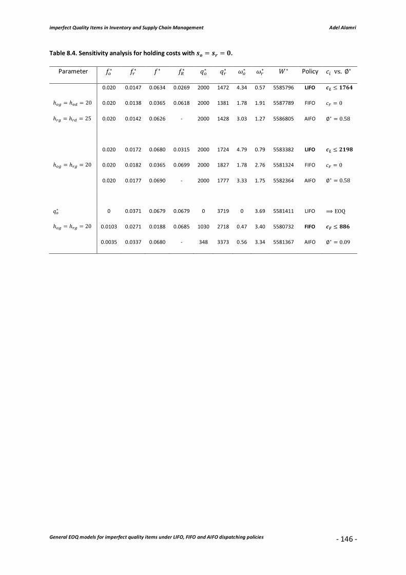
imperfect Quality Items in Inventory and Supply Chain Management Adel Alamri
General EOQ models for imperfect quality items under LIFO, FIFO and AIFO dispatching policies
- 146 -
Table 8.4. Sensitivity analysis for holding costs with 𝒔𝒐 = 𝒔𝒓 = 𝟎.
Parameter 𝑓K∗ 𝑓Ä∗ 𝑓∗ 𝑓L∗ 𝑞K∗ 𝑞Ä∗ 𝜔K∗ 𝜔Ä∗ 𝑊∗ Policy 𝑐Ívs. ∅∗
0.020 0.0147 0.0634 0.0269 2000 1472 4.34 0.57 5585796 LIFO 𝒄𝑳 ≤ 𝟏𝟕𝟔𝟒
ℎK0 = ℎKi = 20 0.020 0.0138 0.0365 0.0618 2000 1381 1.78 1.91 5587789 FIFO 𝑐U = 0
ℎÄ0 = ℎÄi = 25 0.020 0.0142 0.0626 - 2000 1428 3.03 1.27 5586805 AIFO ∅∗ = 0.58
0.020 0.0172 0.0680 0.0315 2000 1724 4.79 0.79 5583382 LIFO 𝒄𝑳 ≤ 𝟐𝟏𝟗𝟖
ℎK0 = ℎÄ0 = 20 0.020 0.0182 0.0365 0.0699 2000 1827 1.78 2.76 5581324 FIFO 𝑐U = 0
0.020 0.0177 0.0690 - 2000 1777 3.33 1.75 5582364 AIFO ∅∗ = 0.58
𝑞K∗ 0 0.0371 0.0679 0.0679 0 3719 0 3.69 5581411 LIFO ⟹ EOQ
ℎK0 = ℎÄ0 = 20 0.0103 0.0271 0.0188 0.0685 1030 2718 0.47 3.40 5580732 FIFO 𝒄𝑭 ≤ 𝟖𝟖𝟔
0.0035 0.0337 0.0680 - 348 3373 0.56 3.34 5581367 AIFO ∅∗ = 0.09

imperfect Quality Items in Inventory and Supply Chain Management Adel Alamri
General EOQ models for imperfect quality items under LIFO, FIFO and AIFO dispatching policies
- 147 -
Table 8.5. Sensitivity analysis for deterioration rates with 𝒔𝒐 = 𝒔𝒓 = 𝟎.
Parameter 𝑓K∗ 𝑓Ä∗ 𝑓∗ 𝑓L∗ 𝑞K∗ 𝑞Ä∗ 𝜔K∗ 𝜔Ä∗ 𝑊∗ Policy 𝑐Ívs. ∅∗
0.020 0.0128 0.0599 0.0235 2000 1285 8.24 0.73 5593672 LIFO 𝑐M = 0
𝑧K = 10 0.020 0.0135 0.0365 0.0611 2000 1348 3.62 3.12 5592737 FIFO 𝒄𝑭 ≤ 𝟏𝟐𝟑𝟔
𝑧Ä = 20 0.020 0.0132 0.0605 - 2000 1318 6.01 1.90 5593230 AIFO ∅∗ = 0.60
𝑞K∗ 0.0097 0.0228 0.0595 0.0418 971 2288 4.84 2.33 5593342 LIFO 𝑐M = 0
𝑧K = 10 0.0134 0.0196 0.0245 0.0603 1343 1959 1.62 3.97 5592454 FIFO 𝒄𝑭 ≤ 𝟕𝟒𝟏
𝑧Ä = 20 0.0117 0.0210 0.0599 - 1173 2108 3.44 3.04 5592887 AIFO ∅∗ = 0.36
0.020 0.0151 0.0641 0.0276 2000 1510 4.28 0.60 5584866 LIFO 𝒄𝑳 ≤ 𝟏𝟗𝟏𝟒
𝛽K = 𝛽Ä = 0 0.020 0.0140 0.0365 0.0622 2000 1406 1.76 1.93 5587011 FIFO 𝑐U = 0
0.020 0.0146 0.0632 - 2000 1458 2.97 1.29 5585950 AIFO ∅∗ = 0.58
0.020 0.0175 0.0687 0.0321 2000 1756 0 0 5576235 LIFO 𝒄𝑳 ≤ 𝟑𝟗𝟔𝟓
𝑙K = 𝑙Ä = 0 0.020 0.0155 0.0366 0.0651 2000 1558 0 0 5580380 FIFO 𝑐U = 0
0.020 0.0165 0.0669 - 2000 1658 0 0 5578342 AIFO ∅∗ = 0.55

imperfect Quality Items in Inventory and Supply Chain Management Adel Alamri
General EOQ models for imperfect quality items under LIFO, FIFO and AIFO dispatching policies
- 148 -
Table 8.6. Sensitivity analysis for special cases of the general models with 𝒔𝒐 = 𝒔𝒓 = 𝟎.
Parameter 𝑓K∗ 𝑓Ä∗ 𝑓∗ 𝑓L∗ 𝑞K∗ 𝑞Ä∗ 𝜔K∗ 𝜔Ä∗ 𝑊∗ Policy 𝑐Ívs. ∅∗
0.020 0.0162 0.0662 0.0297 2000 1525 4.61 0.70 5581490 LIFO 𝒄𝑳 ≤ 𝟏𝟗𝟑𝟗
𝛼 = −500 0.020 0.0153 0.0366 0.0645 2000 1530 1.78 2.19 5583594 FIFO 𝑐U = 0
0.020 0.0158 0.0654 - 2000 1579 3.16 1.47 5586805 AIFO ∅∗ = 0.56
𝑙K = 𝑙Ä = 0 0.020 0.0183 0.0701 0.0335 2000 1833 0 0 5574310 LIFO 𝒄𝑳 ≤ 𝟒𝟏𝟒𝟐
𝛼 = 0 0.020 0.0163 0.0365 0.0664 2000 1631 0 0 5578555 FIFO 𝑐U = 0
𝑎 = 0 0.020 0.0173 0.0683 - 2000 1733 0 0 5576466 AIFO ∅∗ = 0.54
ℎK0 = ℎÄ0 = 20 0.020 0.0161 0.0659 0.0295 2000 1611 4.59 1.15 5584203 LIFO 𝑐M = 0
𝑧Ä = 𝑧K = 20 0.020 0.0161 0.0365 0.0659 2000 1611 1.78 3.96 5584203 FIFO 𝑐U = 0
𝛽K = 𝛽Ä = 25 0.020 0.0161 0.0659 - 2000 1611 3.19 2.55 5584203 AIFO ∅∗ = 0.55
ℎK0 = ℎÄ0 = 20 0 0.0354 0.0648 0.0648 0 3550 a 0 5.4 5585464 LIFO 𝑐M = 0
𝑧Ä = 𝑧K = 20 0 0.0354 0.0648 0.0648 0 3550 a 0 5.4 5585464 FIFO 𝑐U = 0
𝛽K = 𝛽Ä = 25 0 0.0354 0.0648 - 0 3550 a 0 5.4 5585464 AIFO ∅∗ = 0
𝑓K = 0 ⟹ EOQ
a The order quantity as in Example 4.1 (Table 4.2).
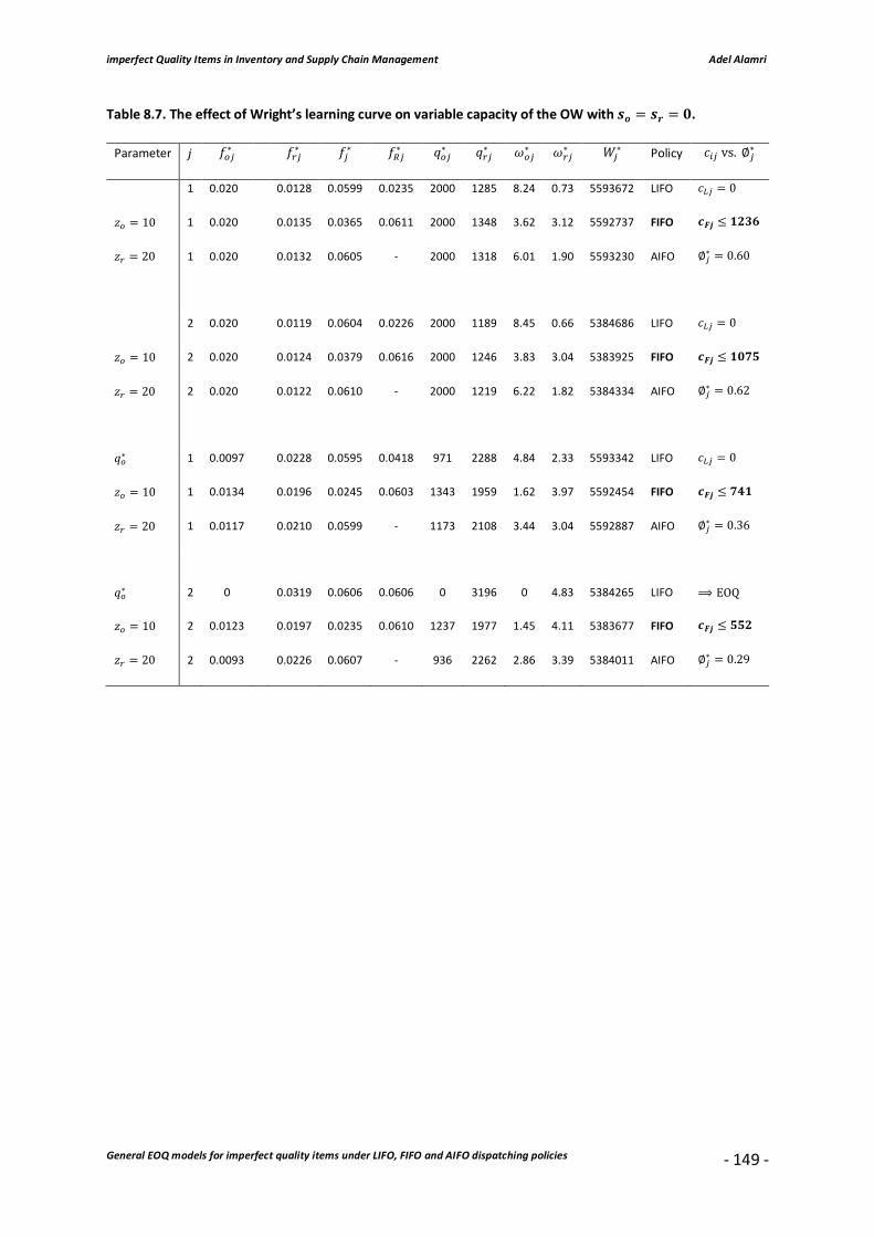
imperfect Quality Items in Inventory and Supply Chain Management Adel Alamri
General EOQ models for imperfect quality items under LIFO, FIFO and AIFO dispatching policies
- 149 -
Table 8.7. The effect of Wright’s learning curve on variable capacity of the OW with 𝒔𝒐 = 𝒔𝒓 = 𝟎.
Parameter 𝑗 𝑓Kd∗ 𝑓Äd∗ 𝑓d∗ 𝑓Ld∗ 𝑞Kd∗ 𝑞Äd∗ 𝜔Kd∗ 𝜔Äd∗ 𝑊d∗ Policy 𝑐Íd vs. ∅d∗
1 0.020 0.0128 0.0599 0.0235 2000 1285 8.24 0.73 5593672 LIFO 𝑐Md = 0
𝑧K = 10 1 0.020 0.0135 0.0365 0.0611 2000 1348 3.62 3.12 5592737 FIFO 𝒄𝑭𝒋 ≤ 𝟏𝟐𝟑𝟔
𝑧Ä = 20 1 0.020 0.0132 0.0605 - 2000 1318 6.01 1.90 5593230 AIFO ∅d∗ = 0.60
2 0.020 0.0119 0.0604 0.0226 2000 1189 8.45 0.66 5384686 LIFO 𝑐Md = 0
𝑧K = 10 2 0.020 0.0124 0.0379 0.0616 2000 1246 3.83 3.04 5383925 FIFO 𝒄𝑭𝒋 ≤ 𝟏𝟎𝟕𝟓
𝑧Ä = 20 2 0.020 0.0122 0.0610 - 2000 1219 6.22 1.82 5384334 AIFO ∅d∗ = 0.62
𝑞K∗ 1 0.0097 0.0228 0.0595 0.0418 971 2288 4.84 2.33 5593342 LIFO 𝑐Md = 0
𝑧K = 10 1 0.0134 0.0196 0.0245 0.0603 1343 1959 1.62 3.97 5592454 FIFO 𝒄𝑭𝒋 ≤ 𝟕𝟒𝟏
𝑧Ä = 20 1 0.0117 0.0210 0.0599 - 1173 2108 3.44 3.04 5592887 AIFO ∅d∗ = 0.36
𝑞K∗ 2 0 0.0319 0.0606 0.0606 0 3196 0 4.83 5384265 LIFO ⟹ EOQ
𝑧K = 10 2 0.0123 0.0197 0.0235 0.0610 1237 1977 1.45 4.11 5383677 FIFO 𝒄𝑭𝒋 ≤ 𝟓𝟓𝟐
𝑧Ä = 20 2 0.0093 0.0226 0.0607 - 936 2262 2.86 3.39 5384011 AIFO ∅d∗ = 0.29

imperfect Quality Items in Inventory and Supply Chain Management Adel Alamri
General EOQ models for imperfect quality items under LIFO, FIFO and AIFO dispatching policies
- 150 -
Fig. 8.5. A comparison of the optimal lot sizes of AIFO and LIFO for S-shaped and Power learning curves.
Fig. 8.6. A comparison of the maximum rental cost per year for S-shaped and Power learning curves.
2 4 6 8 10 12 142900
2950
3000
3050
3100
3150
3200
3250
Numberofcycle
Orderquantity
Q*
AIFO-S-ShapedlearningcurveAIFO-Wright'slearningcurveLIFO-S-ShapedlearningcurveLIFO-Wright'slearningcurve
2 4 6 8 10 12 141380
1390
1400
1410
1420
1430
1440
1450
Numberofcycle
Maximum
rentalcostperyear
CL
LIFO-S-ShapedlearningcurveLIFO-Wright'slearningcurve

imperfect Quality Items in Inventory and Supply Chain Management Adel Alamri
General EOQ models for imperfect quality items under LIFO, FIFO and AIFO dispatching policies
- 151 -
In the next section, we list some key findings that depict the behaviour of the theoretical
models in different realistic scenarios and we further relate the results of our work to the
general body of knowledge in the discipline.
8.8.5. Findings
• For any 𝑠K = 𝑠Ä ≥ 0, the optimal order quantity is identical for each model, which
signifies the importance of considering differing transportation costs in the
mathematical formulation of two-warehouse inventory models (Table 8.3).
• The dis-location of good and defective items significantly influences the optimal order
quantity (Tables 8.3 and 8.4).
• The assumption that the OW is fulfilled with the maximum capacity is indeed not the
optimal choice for specific input parameters (Tables 8.3, 8.4, 8.5 and 8.7). Although
such finding may appear to be counterintuitive, it is indeed an important finding for
practitioners, since the objective is to minimise the total system cost.
• Under FIFO and LIFO policies, it may become optimal that no items are stored in the
OW, i.e. the problem reduces to the EOQ (Tables 8.3, 8.4 and 8.7), which is consistent
with the behaviour of outsourcing inventory holding through a vendor managed
inventory (VMI) or other inventory intermediary arrangement (Table 8.6).
• Relaxing the inherent determinism of the maximum capacity associated with OW, not
only produces better results, but may also reduce the value of the upper-bound
significantly (Tables 8.4, 8.5 and 8.7).
• For equal holding costs and deterioration rates, the optimal order quantity for the
three models is identical, i.e. 𝑐Í = 0, which implies that LIFO (AIFO) is optimal if and
imperfect Quality Items in Inventory and Supply Chain Management Adel Alamri
General EOQ models for imperfect quality items under LIFO, FIFO and AIFO dispatching policies
- 152 -
only if 𝑐Í = 0 (Table 8.6). This finding is fundamental, since it not only shows the
validity and robustness of the proposed models, but also underpins and portrays the
value added for integrating the upper-bound in the mathematical formulations.
• Table 8.6 reveals that when 𝑓K = 0, all models are reduced to a single-level warehouse
base model presented in Chapter 4 (Alamri et al. (2016). In this case, 𝑐Í = 0, which
also shows the validity and robustness of the proposed models.
• It should be noted that the results presented in Table 8.2 reveal that the reduction in
the optimal order quantity does not affect the OW. That said, although the OW may
benefit from the VOI that reduces the defective items per lot, it still retains the
maximum capacity of goods and, consequently, the effect of learning does not really
apply here. On the other hand, this is not the case when relaxing the inherent
determinism of the maximum capacity associated with OW. In particular, such
relaxation implies comprehensive learning that can be achieved simultaneously, i.e.
the amounts that are allocated to both the OW and RW are affected (Table 8.7).
However, and despite the fact the lot size may reduce for each successive
replenishment, the amount that is allocated to the OW either remains static (due to
capacity restriction) or experiences further reduction, but the amount that is allocated
to the RW may decrease (increase) subject to the input parameter. This is a key
finding, which demonstrates the impact of learning on the operational and financial
performance of an inventory system with a two-level storage.
• Fig. 8.5 indicates that the optimal order quantity of AIFO and LIFO follows the same
fashion as that of 𝑝d.
• The same behaviour observed in Fig. 8.5 holds true for the total minimum costs per
year, which can be further justified by the reduction gained in the maximum rental

imperfect Quality Items in Inventory and Supply Chain Management Adel Alamri
General EOQ models for imperfect quality items under LIFO, FIFO and AIFO dispatching policies
- 153 -
cost per year (upper-bound) (Fig. 8.6).
• The S-shaped logistic learning curve generates greater quantities in the incipient
phase, which is consistent with the behaviour of slow improvement that is observed
in practice (Dar-El, 2000).
• Previously published models in this area are shown to be special cases of our models
(Table 8.6, Appendix B, Appendix C and Appendix D).
Remark 8.1
The proposed models are not limited to the above contributions; the versatile nature of our
models and the fact that they may trigger other applications that can be disseminated from
the general formulation is shown in Section 8.9 below.
8.9. Special cases of the general EOQ models
In this section, we offer a number of special cases to illustrate the theoretical application of
our mathematical models. We aim to address the quality related issues discussed in Chapters
2 and 5 when formulating LIFO and FIFO EOQ models for items that require 100 per cent
screening. In particular, we show that the special cases covered in Chapter 5 can be easily
addressed for LIFO and FIFO, although many of these issues have neither been recognised nor
analytically examined before. Moreover, the interface between different transportation costs
associated with OW and RW and the upper-bound (cost applied if OW (RW) is idle) allows
inventory managers to compare between LIFO, FIFO and AIFO dispatching policies to establish

imperfect Quality Items in Inventory and Supply Chain Management Adel Alamri
General EOQ models for imperfect quality items under LIFO, FIFO and AIFO dispatching policies
- 154 -
the optimum order quantities that minimise the total system cost.
The remainder of the section is organised as follows: First, we provide a brief summary of
general solution procedures for managing perishable products and lifetime constraints,
followed by linking our mathematical formulations to the renewal theory, whereby we show
that previously published models in this area constitute special cases of our models.
8.9.1. Perishable products and lifetime constraints
The implication of the inspection process into inventory decision-making can be further
explored to accommodate an inventory system with a two-level storage. Specifically, a lot of
size 𝑄Íd = 𝑞KÍd + 𝑞ÄÍd is delivered such that a quantity of size 𝑞KÍd is allocated to the OW and
the remaining amount of size 𝑞ÄÍd = 𝑄Íd − 𝑞KÍd is allocated to the RW. The assumption that
each sub-replenishment that enters the RW undertakes a 100 per cent screening would imply
that 𝑞ÄÍd = e𝑞ÄÌd, 𝑞ÄÌ/jd ,… , 𝑞Äqdf where 𝑞Ä6d is the number of units with 𝑘(𝑘 = 0,1, … ,𝑚)
useful periods of shelf lifetime. Here, 𝑞Äqd denotes newly replenished items that have arrived
already perished or items not satisfying certain quality standards (defective items). A similar
argument holds true for the quantity 𝑞KÍd that is allocated to the OW. Although no buyer
would pay for defective and already perished items, they would surely be interested in seeing
a reduction in the presence of such quantities in subsequent replenishments. Our formulation
allows for an immediate disposal of the amount 𝑞Äqd + 𝑞Kqd in case of any potential safety
issues, i.e. ℎKi = ℎÄi = 0. Now, let 𝜔Ä6d denote the quantity of the on-hand inventory of
shelf lifetime 𝑘 that perishes by the end of period 𝑘 in RW. Thus, we have

imperfect Quality Items in Inventory and Supply Chain Management Adel Alamri
General EOQ models for imperfect quality items under LIFO, FIFO and AIFO dispatching policies
- 155 -
𝜔Ä6d = }𝑞Ä6d − t𝐷6d − e∑ 𝑞Ä@d6/j@Ôj − ∑ 𝜔Ä@d6/j
@Ôj − ∑ 𝑑Ä@d6@Ôj fu¸
0otherwise,
where 𝐷6d < e∑ 𝑞Ä@d6@Ôj − ∑ 𝜔Ä@d6/j
@Ôj − ∑ 𝑑Ä@d6@Ôj f is the actual demand observed up to the
periodic review 𝑘, and 𝑑Ä6d is the number of items of shelf lifetime 𝑘 that deteriorate in RW
while on storage. Hence, ∑ 𝑑Ä×dÌ×Ô6 denotes the total sum of deteriorated items in RW in
period 𝑘, i.e. an item may not retain the same utility throughout its shelf lifetime, and
consequently ∑ 𝜔Ä6dÌ6Ôj refers to the total sum of inventory in RW that perishes in cycle 𝑗,
excluding any replenished items that have arrived already perished. A similar argument holds
true for the quantity 𝜔K6d that perishes in OW. It is important to note that if LIFO or FIFO are
considered, then ∑ 𝜔Ä6dÌ6Ôj + ∑ 𝜔K6dÌ
6Ôj is likely greater than that experienced under the
AIFO policy. This can be justified by the marginal difference in cycle length (Sections 8.8.2 and
8.8.4) and the fact that under the LIFO and FIFO policies, only one warehouse is utilised at a
time. This is an important issue, especially in the case when a distinct selling price 𝑣6 may be
linked to its corresponding quantity 𝑞6d, i.e. 𝑉 = (𝑣Ì,𝑣Ì/j, … ,𝑣q)is applied for the set 𝑄Íd =
e𝑞Ìd, 𝑞Ì/jd ,… , 𝑞qdf. Therefore, our formulation is viable if, for instance, an item partially
loses its value based on its perceived actuality (obsolescence).
The above discussion further underpins and demonstrates how the terms “deterioration”,
“perishability” and “obsolescence” may collectively affect inventories in a two-level storage.
Note that 𝑚Ír can still be used to drive the optimal quantity that needs to be added to the
on-hand inventory for the next replenishment, i.e. 𝑞Í6d = 𝑄Íd¸j−𝐼K0Íde𝑡6df − 𝐼Ä0Íde𝑡6df,
where 𝑡6d denotes the time up to the periodic review. This relation holds true for Sections
6.5.1, 7.5.1, 8.8.2 and 8.8.4, i.e. 𝑞d = 𝑄d − 𝐼K0d/je𝑇d/jf − 𝐼Ä0d/je𝑇d/jf for AIFO and LIFO and
𝑞d = 𝑄d − 𝐼K0d/je𝑇Ld/jf − 𝐼Ä0d/je𝑇Ld/jf for FIFO. Therefore, similar arguments as those for
imperfect Quality Items in Inventory and Supply Chain Management Adel Alamri
General EOQ models for imperfect quality items under LIFO, FIFO and AIFO dispatching policies
- 156 -
Sections 5.2 and 5.3 can be implemented here.
As an example of lifetime constraint, we can assume that Τ denotes the remaining shelf
lifetime of an item and ℃×and𝑡× represent, respectively, the temperature and time elapsed
of an item in a supply chain entity 𝑦. Then we have Τ = 𝑀 − 𝜁(℃ï)𝑡ï − 𝜁(℃ð)𝑡ð, where
𝜁e℃×f = (0.1℃× + 1)rand𝑀 = 𝑚 + 𝑡ï + 𝑡ð (Bremner, 1984; Ronsivalli and Charm, 1975).
In this case, 𝑓d ≤ Τ for AIFO and LIFO and 𝑓Ld ≤ Τfor FIFO, and consequently, the VOI can be
quite valuable in reducing the cost per cycle (Chapter 5). Note that 𝑧× = 1 + Τ can also fit
here.
8.9.2. Stochastic parameters
Let 𝑋d refer to a set of random variables that are predetermined according to the VOI gained
by the system due to its coordination as an output of the 𝑗1� inspection process. Suppose that
𝑋d~𝑈 z𝑌d − √3𝑍d,𝑌d + √3𝑍d{. Note that 𝐸 A𝑋dG = 𝑌d, i.e. if 𝐷d~𝑈t𝜇d − √3𝜎d,𝜇d + √3𝜎du,
then 𝐸(𝐷d) = 𝜇d = 𝐷(𝑡) = 𝑟. A similar argument holds true for other input parameters.
Note that 𝑋d and hence the actual yield may vary from one cycle to another (e.g. the
parameters are nonstationary). Thus, we have 𝐸(𝑊Í) =ù(�Ú)ùe�Úmf
=ùA�ÈÅm
� G
ùÏ�m,ÈÅm� Ñ
, for AIFO and LIFO,
and 𝐸(𝑊U) =ù(�V)ùe�Omf
=ùA�ÈÅm
� G
ùÏ�Om,ÈÅm� Ñ
,for FIFO, wheree1 − 𝐸t𝑝duf𝑥(𝑡) > 𝐷(𝑡).
In the example provided by Jaggi et al. (2015), it is assumed 𝐸[𝑝] = 0.02, 𝑞K = 800, ℎK0 =
ℎKi = 5, ℎÄ0 = ℎÄi = 7, 𝛽K = 𝛽Ä = 0, 𝑐 = 25, 𝑘 = 100, 𝑟 = 50000, 𝑙K = 𝑙Ä = 1, 𝑧K =

imperfect Quality Items in Inventory and Supply Chain Management Adel Alamri
General EOQ models for imperfect quality items under LIFO, FIFO and AIFO dispatching policies
- 157 -
3.33, 𝑧Ä = 5, 𝛼 = 0and𝑏 = 175200, resulting in 𝑄(¿1ïÛ = 915units. This quantity is
greater than our optimal 𝑄M∗ = 909unitsand𝑤M∗ = 1312381dollars. However, 𝑄U∗ =
943unitsand𝑤U∗ = 1312315, and consequently FIFO performs better than LIFO. Moreover,
if 𝑞K is taken as a decision variable, then 𝑞K∗ = 0,𝑄M∗ = 920unitsand𝑤M∗ =
1312126dollars ⟹ the solution of FIFO does not exist. This result is consistent with the
results obtained in Tables 8.3, 8.4, 8.5 and 8.7 and seems realistic, given that the objective is
to minimise the total system cost. Setting 𝑙K = 𝑙Ä = 0, the result is identical with that of
Chung et al. (2009) and Jaggi et al. (2015), where 𝑄M∗ = 𝑄l ¿1ïÛ = 𝑄(¿1ïÛ = 1290units.
In the next section, we summarise the implications and managerial insights of our work and
relate the results of the study to the general body of knowledge in the discipline. Further, we
emphasise the fact that each model may trigger other applications that can be disseminated
from the general formulation.
8.10. Summary of implications and managerial insights
• The versatile nature of each model allows the incorporation of the desired functions
that are suitable to a system. Consequently, the list of implications and managerial
insights outlined in Section 5.9 fits our models as well.
• Each model emerges as a viable solution that manages and controls the flow of
perishable and non-perishable products so as to reduce cost and/or waste for the
benefit of economy, environment and society.
• General solution procedures for LIFO, FIFO and AIFO to determine the optimal
dispatching policy for continuous intra-cycle periodic review applications for two-level
imperfect Quality Items in Inventory and Supply Chain Management Adel Alamri
General EOQ models for imperfect quality items under LIFO, FIFO and AIFO dispatching policies
- 158 -
storage EOQ models are presented. The proposed solution procedures consider
different inventory fluctuations during the planning horizon.
• A detailed method to illustrate how deterioration, perishability and obsolescence may
collectively affect inventories in a two-level storage is explored.
• The accuracy of RFID temperature tags that capture the TTH, and the use of that TTH
data are adopted to model the shelf lifetime of an item under LIFO, FIFO and AIFO
dispatching policies.
• The mathematical formulations are linked to the renewal theory to show that
previously published models in this area constitute special cases of our models.
• The importance of considering differing transportation costs in the mathematical
formulation of two-warehouse inventory models is illustrated.
• The assumption that the OW is fulfilled with the maximum capacity is indeed not the
optimal choice for specific input parameters, which constitutes an important decision
for practitioners, since the objective is to minimise the total system cost.
• Relaxing the inherent determinism of the maximum capacity associated with OW, not
only produces better results, but may also suggest an alternative policy and reduce
the value of the upper-bound significantly. Moreover, it implies comprehensive
learning that can be achieved simultaneously, i.e. the amounts that are allocated to
both the OW and RW are affected, which demonstrates the impact of learning on the
operational and financial performance of an inventory system with a two- level
storage.
• Integrating the upper-bound in the mathematical formulations of LIFO and FIFO
models, i.e. the introduction of a KPI to trade-off the costs associated with AIFO, LIFO
and FIFO policies constitutes a key business objective in supply chain management.

imperfect Quality Items in Inventory and Supply Chain Management Adel Alamri
General EOQ models for imperfect quality items under LIFO, FIFO and AIFO dispatching policies
- 159 -
• Under FIFO and LIFO policies, it may become optimal that no items are stored in the
OW, which suggests an outsourcing inventory holding through a VMI or other
inventory intermediary arrangement.
• In the case of managing perishable products, LIFO and FIFO may not be the right
dispatching policies, given that the order quantity needs to be consumed based on a
FEFO policy. This is so, since under the LIFO or FIFO dispatching polices, the total sum
of inventory that perishes in each cycle is likely greater than that experienced under
the AIFO policy.
• The dimension of risk influencing the management of perishable products may
increase if, for instance, a distinct selling price is linked to its corresponding quantity
with a distinct useful period of shelf lifetime.
• Under an AIFO dispatching policy, a discounted holding cost can be gained if a
continuous and long-term rental contract is beneficial and hence further reduction in
the total minimum cost per year can be achieved.
8.11. Conclusion and further research
In this chapter, we have been concerned with the implications of dispatching policies
associated with a two-level storage, where each lot is subjected to a 100 per cent screening.
Three general EOQ models for items with imperfect quality were presented and compared.
The first model underlies LIFO, the second model underlies FIFO and the third model relates
to simultaneous consumption fractions associated with OW and RW and is entitled Allocation-
In-Fraction-Out (AIFO). Under an AIFO dispatching policy, the cycle length is the same for both
OW and RW, and consequently the upper-bound (cost applied if OW (RW) is idle) that renders

imperfect Quality Items in Inventory and Supply Chain Management Adel Alamri
General EOQ models for imperfect quality items under LIFO, FIFO and AIFO dispatching policies
- 160 -
AIFO the optimal dispatching policy has also been provided. It has been shown that the
solution to AIFO inventory model, if it exists, is unique and global optimal. Items not
conforming to certain quality standards are isolated in separate facilities with different
holding costs of the good and defective items being considered.
The analytical results illustrate the impact of considering different transportation costs
associated with OW and RW, as well as the incorporation of varying demand, deterioration,
defectiveness and screening rates on the optimal order quantity. Relaxing the inherent
determinism related to the maximum capacity of OW not only produces better results, but
may also reduce the value of the upper-bound significantly. If the system is subject to
learning, then this relaxation implies further reduction in the quantity allocated to the OW
for each successive sub-replenishment that is delivered to OW, i.e. the system experiences
comprehensive and simultaneous learning.
This study is viable for fixed and random lifetimes of perishable products, where VOI is
adopted to model the shelf lifetime of an item. The versatile nature of our models and the
fact that they may reflect a diverse range of strategies has been emphasised, whereby the
validity of the general models is ascertained, i.e. the solution is the same as in published
sources or in some cases produces better results. To the best of our knowledge, this appears
to be the first time that such an Allocation-In-Fraction-Out (AIFO) policy is presented, which
necessitates a general formulation of LIFO and FIFO EOQ models for investigation and
numerical comparison purposes.
Further research can be addressed for finite or infinite planning horizons that may include
extensions, such as allowing for shortages, considering that the screening rate follows
learning and forgetting curves, and the risk of failure during screening (Type I and Type II

imperfect Quality Items in Inventory and Supply Chain Management Adel Alamri
General EOQ models for imperfect quality items under LIFO, FIFO and AIFO dispatching policies
- 161 -
errors). In addition, it appears plausible to assess the formulation of EOQ models for a two-
level storage to consider multiple items or to study the effect of different supplier trade credit
practices.

imperfect Quality Items in Inventory and Supply Chain Management Adel Alamri
Part D
- 162 -
Part D: Conclusion
This part consists of the last chapter of our work. In this chapter (Chapter 9), we highlight the
overall contributions, findings and implications, and managerial insights presented in this PhD
thesis. This chapter closes with a discussion of further research.

imperfect Quality Items in Inventory and Supply Chain Management Adel Alamri
Summary of contributions and further research
- 163 -
9. Summary of contributions and further research
9.1. Introduction
In this chapter, we highlight the overall contributions and findings presented in this PhD
thesis, summarise the implications and managerial insights of our work, relate the results of
the study to the general body of knowledge in the discipline and provide a discussion of
natural avenues for further research.
Inventory management is a field which has been relatively mature for several decades.
Moreover, there is no single existing theory that can adequately capture all aspects of the
relevant processes and the inventory problems associated with them. Therefore, making a
contribution that scholars would deem “significant” is not an easy task.
In this PhD thesis, we have attempted to advance the current state of knowledge in the field
of inventory mathematical modelling and management by means of providing theoretically
valid and empirically viable generalised inventory frameworks to assist inventory managers
towards the determination of optimum order/production quantities that minimise the total
system cost. From a theoretical perspective, the generic nature of our models enables the
decision maker to incorporate a diverse range of strategies that may reflect many real-world
concerns. From a practitioner’s perspective, this PhD thesis generated interesting managerial
insights. Despite the obvious implications that are triggered by the general formulations and
the fact that many practical examples published in the literature for generalised models in
this area constitute special cases of our proposed models, the following objectives were also
considered, for the first time, in this work:
imperfect Quality Items in Inventory and Supply Chain Management Adel Alamri
Summary of contributions and further research
- 164 -
1) To explore the implications of the inspection process on inventory decision-making and link
such process with the management of perishable inventories;
2) To derive a general, step-by-step solution procedure for continuous intra-cycle periodic
review applications;
3) To demonstrate how the terms “deterioration”, “perishability” and “obsolescence” may
collectively apply to an item;
4) To develop a new dispatching policy that is associated with simultaneous consumption
fractions from an owned warehouse (OW) and a rented warehouse (RW). The policy
developed is entitled “Allocation-In-Fraction-Out (AIFO)”;
5) To relax the inherent determinism related to the maximum fulfilment of the capacity of
OW to maximising net revenue; and
6) To assess the impact of learning on the operational and financial performance of an
inventory system with a single-level storage and a two-level storage.
9.2. Models overview
In this section, we emphasise the practical application of our work, where each model is based
on a single item held in stock, whether this item is perishable or non-perishable. This means
that each model is applicable in contexts such as grocery retailing, armed forces, hospitals,
wholesaling, manufacturing, etc.
Below, 3 single item examples (grocery retailer, hospital and manufacturer) are given
imperfect Quality Items in Inventory and Supply Chain Management Adel Alamri
Summary of contributions and further research
- 165 -
illustrating the applicability and importance of the models.
Case 1: Suppose that a grocery retailer is purchasing a seasonal product say, Indian mango.
Assume that the demand rate for such product is considered, respectively, to be linearly
increasing with time in the first three replenishments (what would more generally correspond
to the growth stage of the life cycle of the product, i.e. customers are likely to buy mango),
constant for the following two replenishments (in the mature stage of the life cycle of the
product) and linearly decreasing with time in the last two replenishments (in the declining
stage of the life cycle of the product, i.e. few customers are likely to buy mango).
The lot size shipment that enters the sorting facility consists of cartons of mangos worth 8
dollars each and contains six pieces. Since customers normally check many cartons before
they pick the right one, the lot size shipment undertakes 100 per cent inspection. In this case,
inspection reduces the potential rejection that could happen because of one defective piece
of mango that could be easily replaced with a good one in the same carton. In addition,
inspection can be used to classify those cartons based on some sort of presentation, price or
freshness in order to reduce waste and/or maximise revenue. Moreover, any defective piece
of mango may affect other pieces and thus increases potential waste. All defective complete
cartons and/or pieces of mangos can be sold at a salvage price or even incur a disposal cost.
As time goes on, the rate of deterioration increases due to the change in the physical status
of mangos. In addition, customers randomly, check many cartons before they pick the right
one, i.e. they may touch some mangos in the cartons, which in turn increases the rate of
deterioration as many more costumers have checked the same cartons.
imperfect Quality Items in Inventory and Supply Chain Management Adel Alamri
Summary of contributions and further research
- 166 -
In this case, i.e. Case 1, an inventory system with a two-level storage (OW and RW) applies, if
for example, the grocery retailer may have been enticed with price discounts to purchase a
number of cartons of mangos that exceed the limited capacity of OW. In this case, the grocery
retailer can trade-off between AIFO, LIFO and FIFO to find the best dispatching policy.
Case 2: Suppose that a hospital receives a seasonal flu medicine, say drug X (Vaccine), which
is liquid in nature. Assume that the demand rate for such medicine is considered to be linearly
increasing with time. The lot size shipment that enters the warehouse consists of cartons of
drug X, each of which may have a different expiration date as a result of a dispatching policy
embraced by the supplier. In this case, and to reduce any potential risk of perishability, the
lot size shipment undertakes 100 per cent inspection so as to classify those cartons into two
categories, say long-term and short-term dispatching policies (FEFO). Any cartons with
remaining shelf life time less than, say six months are considered to be defective as per the
regulation of say, Ministry of Health that the supplier agrees upon. All defective complete
cartons are sent back to the supplier and all damaged bottles of drug X are also considered
defective and may incur a disposal cost.
Demand, say for three different pharmacies in the hospital is satisfied from inventory of short-
term category first, then demand is satisfied from inventory of long-term category. As time
goes on, some bottles of drug X may get damaged while they are on storage and some others
may experience misplacement by pharmacists, nurses or doctors such that the minimum
remaining shelf life time of six months is no longer valid when such bottles are found. All
bottles of drug X that do not meet the minimum remaining shelf life time of six months are
considered deteriorated and must sent back to the supplier. All damaged bottles of drug X
imperfect Quality Items in Inventory and Supply Chain Management Adel Alamri
Summary of contributions and further research
- 167 -
are also considered deteriorated and may incur a disposal cost.
In this case, i.e. Case 2, classifying cartons into two categories, i.e. long-term and short-term
and, the fact that the demand is satisfied from inventory of short-term category first, then
demand is satisfied from inventory of long-term category involves a straightforward
application of either LIFO or FIFO dispatching policies. This implies that inventory of short-
term category (theoretically stored in (OW or RW)) is consumed first, before considering
inventory of long-term category (theoretically stored in (RW or OW)), i.e. an inventory system
with a two-level storage applies here. Another application of an inventory system with a two-
level storage occurs, if for instance, the lot size shipment may be allocated to two warehouses
due to capacity restriction of one warehouse.
Case 3: Suppose that a manufacturer purchases returned products, say product Y (lithium
battery) as well as three different new components that are required in a production setting.
Inventory of returned products is stored in a separate shop (warehouse). Assume that the
demand rate for such product follows a production rate that is considered to be linearly
increasing with time.
The lot size shipment of returned products that enters the warehouse consists of batteries
each of which has three different usable functional components. In this case, the lot size
shipment of returned products undertakes 100 per cent inspection, where each battery is
disassembled to isolate usable functional components to be transferred in batches to the
production shop. All defective batteries and/or unusual functional components can be sold
as scrap or even incur a disposal cost.

imperfect Quality Items in Inventory and Supply Chain Management Adel Alamri
Summary of contributions and further research
- 168 -
Each transferred batch contains distinct usable functional components, which represent a
fraction of the demand and the rest is satisfied from inventory of new components. As time
goes on, some batteries may get totally damaged while they are on storage and some damage
may also affect some functional components. All totally damaged batteries and unusual
functional components can be sold as scrap or even incur a disposal cost.
In this case, i.e. Case 3, an inventory system with a two-level storage (OW and RW) applies, if
for example, it is cost effective for the manufacturer to purchase a number of batteries that
exceed the limited capacity of OW. In this case, the manufacturer can trade-off between AIFO,
LIFO and FIFO to find the best dispatching policy.
9.3. Lot size inventory model with one level of storage
9.3.1. Research contribution
In this section, we summarise and emphasise the financial implications and managerial
aspects of our work in the case of a single storage. Opportunities and challenges in this case
include poor supplier service levels (imperfect items received from suppliers), potential dis-
location of good and defective items (different warehouses for the good and defective items),
goods’ deterioration during storage and transfer of knowledge from one inventory cycle to
another.
The combination of such challenges/opportunities is important in many industries and may
significantly influence the optimal order quantity. This is an important issue especially in the
case of managing perishable products where inspection would imply that products may be
classified according to quality, size, appearance, freshness, etc., and where a distinct selling

imperfect Quality Items in Inventory and Supply Chain Management Adel Alamri
Summary of contributions and further research
- 169 -
price may be linked to its corresponding quantity. Moreover, inspection may eliminate the
return service cost associated with product recalls. In real-life settings, the impact of allowing
through defective items could be severe (Klassen and Vereecke 2012). The service cost may
include goodwill cost, transportation cost, and re-processing cost, and that may affect all
supply chain members. Inspection may also reduce holding costs due to the deployment of
less preserving environmental conditions, i.e. the defective items are not usually stored in the
same warehouse where the good items are stored (e.g. Wahab and Jaber, 2010). Inspection
may also be presumed essential for updating the Information System records with good items
that are actually available in stock, so as to avoid shortages. Moreover, a 100 per cent
inspection will render a potential random lifetime of a product deterministic, i.e. it intersects
the areas of fixed and random lifetimes of an item. Finally, inspection not only isolates
defective and/or already perished items, but also leads to the consumption of the order
quantity based on a FEFO policy. For example, isolation, i.e. dis-location of good and defective
items, allows for an immediate disposal of defective and/or already perished items in case of
any potential safety issues.
The generality of our model stems from the fact that the demand, screening, and product
deterioration rates are arbitrary functions of time. The proposed model unifies and extends
the academic literature related to imperfect quality items, which is comparatively diverse in
nature. Mathematical proof was presented, which shows that the solution to the underlying
inventory model, if it exists, is unique and global optimal. It has been shown that practical
examples published in the literature for generalised models constitute special cases of our
model. This implies that the solution is the same as in published sources or in some cases
produces better results, which indicates that the validity of the general model is ascertained.
imperfect Quality Items in Inventory and Supply Chain Management Adel Alamri
Summary of contributions and further research
- 170 -
The versatile nature of our model, and the fact that it may accommodate many real-world
concerns, has been emphasised in that the results obtained are compatible with the
behaviour observed in many real-life settings. The obtained numerical results support
application of the model and solution procedure in different realistic situations. For example,
the presence of product deterioration and varying demand and screening rates significantly
impact on the optimal order quantity. However, a reduction in the optimal order size does
not necessarily lead to a lower total minimum cost per unit time. Moreover, we extended
upon the financial implications and managerial insights of our work by offering a number of
special cases to illustrate the theoretical application of our general model.
The mathematical formulation of our model intersects the areas of fixed and random lifetimes
of perishable products, whereby the value of the temperature history and flow time through
the supply chain is also used to determine an appropriate policy. Furthermore, it provides a
general procedure for continuous intra-cycle periodic reviews so as to adjust and control the
flow of raw materials, component parts and finished goods to maintain sustainable
competitive advantage. Coordination mechanisms and managerial decision strategies that
govern both the supplier and the retailer were also addressed to improve inventory
management at both echelons.
We tested and observed the behaviour of varying demand, screening, defectiveness and
deterioration rates, VOI and perishable and non-perishable (infinite shelf lifetime) items that
are subject to deterioration while in storage. The resulting insights offered to inventory
managers are considered to be of significant value, since many of these issues have not been
previously investigated. Therefore, the model emerges as a viable solution that manages and
controls the flow of perishable and non-perishable products.
imperfect Quality Items in Inventory and Supply Chain Management Adel Alamri
Summary of contributions and further research
- 171 -
Below, we list some key findings that depict and emphasise the behaviour of the theoretical
model in different settings and relate the results of the study to the general body of
knowledge in the discipline.
9.3.2. Key Findings
• The total minimum cost per unit time and the total minimum cost per cycle decrease
as learning increases, which supports the findings presented by Wahab and Jaber
(2010).
• As learning increases, all optimal quantities decrease, except for the amount of
deteriorated items that incur a minor increase that can be justified by the slight
increase in the cycle length.
• The presence of defects and varying demand and deterioration rates significantly
impact on the optimal order quantity.
• The lot size with the same assumed holding costs for the good and defective items is
less than the one with differing holding costs. However, the difference between the
two quantities vanishes as 𝑝d takes on relatively small values. Such finding is
consistence with that presented by Wahab and Jaber (2010).
• The results show a slight decrease in the total minimum cost per unit time due to a
slight decrease in 𝑝d. This is true in the incipient phase when an S-shaped logistic
learning curve is assumed, which is consistent with the behaviour of slow
improvement observed in this short phase, making the S-shaped learning curve an
appropriate model to use (Dar-El, 2000). On the other hand, this is not the case when
Wright’s learning curve is considered, which then leads to smaller quantities in the
incipient phase and hence the total minimum cost per unit time behaves similarly.
imperfect Quality Items in Inventory and Supply Chain Management Adel Alamri
Summary of contributions and further research
- 172 -
• The reduction in the total minimum cost per unit time and the optimal order
quantities follow the same fashion as that of 𝑝d.
• The effect of 𝛼, the rate of change in the demand significantly influences the optimal
order quantity and the total minimum cost per unit time.
• The presence of deterioration has a significant impact on the optimal order quantity
and the total minimum cost per unit time. Such finding is consistence with that
presented by Moussawi-Haidar et al. (2014).
9.3.3. Implications and managerial insights
In this section, we summarise the implications and managerial insights of our work and relate
the results of the study to the general body of knowledge in the discipline.
• The generic nature of our model allows incorporation of the desired functions that are
suitable to a system.
• A general step-by-step solution procedure to determine the optimal policy for
continuous intra-cycle periodic review applications is presented, which is valid for the
generalised models and can be further extended to be implemented in inventory
mathematical modelling. Moreover, the structure of the model allows for both
continuous and discrete periodic review.
• Clearer definitions that are associated with the terms deterioration, perishability and
obsolescence are suggested in order to refine and distinguish the role of each term
for the model. In addition, a detailed method was also provided, which underpins and
portrays how these terms may collectively apply to an item.
imperfect Quality Items in Inventory and Supply Chain Management Adel Alamri
Summary of contributions and further research
- 173 -
• The proposed model intersects the areas of fixed and random lifetimes of perishable
products. Moreover, it is viable for the case in which items are classified based on their
quality, size, appearance, freshness, etc., whereby the dis-location of good and
defective items allows for an immediate disposal of defective and/or already perished
items in case of any potential safety issues.
• The proposed model emerges as a viable solution that manages and controls the flow
of perishable and non-perishable products in order to reduce cost and/or waste for
the benefit of economy, environment and society.
• The VOI can be perceived at external and/or internal domains of coordination. At the
domain of external coordination, the integration of the VOI captures a safe remaining
shelf lifetime. For example, the accuracy of RFID temperature tags that capture the
TTH data are adopted to model the shelf lifetime of an item. At the domain of external
and internal coordination, the presence of the VOI acknowledges the potential impact
of transporting and handling a product through the supply chain. In this case, any
information gained from previous replenishments can be incorporated to reduce the
presence of both defective and already perished items in subsequent replenishments.
• The versatile nature of our model accommodates renewal theory, stochastic process
and inspecting a random sample size drawn from the batch, where input parameters
are randomly distributed. It also accounts for the case when subsequent
replenishment is cycle dependent. This line of research was also enhanced, whereby
coordination mechanisms and managerial decision strategies that govern both the
supplier and the retailer are addressed to improve inventory management at both
echelons.

imperfect Quality Items in Inventory and Supply Chain Management Adel Alamri
Summary of contributions and further research
- 174 -
9.4. Lot size inventory model with two levels of storage
9.4.1. Research contribution
In this section, we highlight research contribution and summarise the theoretical application,
financial implications of dispatching policies associated with a two-level storage and
managerial aspects related to our findings.
The contribution of this work goes beyond addressing the practical concerns with regards to
product quality related issues that are linked with the opportunities raised in Section 9.2.1
when formulating a two-warehouse inventory model for items that require 100 per cent
screening. In particular, a new policy entitled “Allocation-In-Fraction-Out (AIFO)” was
developed. Under an AIFO dispatching policy the goods at RW and OW experience
simultaneous consumption fractions, which implies that the inventories at both warehouses
are depleted by the end of the same cycle. On the other hand, the LIFO and FIFO policies
assume no cost effect while the initially used warehouse is idle, which is unrealistic and a rare
scenario to encounter in practice. Subsequently, this necessitated introducing costs
associated with the OW or RW being idle when formulating a two-warehouse inventory
model. Therefore, three general EOQ models for items with imperfect quality were presented
and compared. The first model underlies the LIFO policy, the second model underlies the FIFO
policy and the third model relates to the AIFO policy.
It becomes apparent that the tradeoff between the three policies constitutes a key business
objective in supply chain management. Under both the LIFO and FIFO dispatching policy, the
cost associated with the OW or RW being idle is treated as an input parameter as well as a
decision variable. If the cost is a decision variable, then it constitutes a KPI, i.e. an upper-

imperfect Quality Items in Inventory and Supply Chain Management Adel Alamri
Summary of contributions and further research
- 175 -
bound (cost associated with OW (RW) being idle) that renders AIFO the optimal dispatching
policy.
To the best of our knowledge, the maximum capacity of the OW is invariably treated in the
academic literature as an input parameter. Relaxing the inherent determinism related to the
maximum fulfilment of the capacity of OW may lead to maximizing net revenue. In addition,
if the system is subject to learning, then the lot size may reduce for each successive
replenishment. However, such reduction affects the amount allocated to the RW only, and
the amount allocated to the OW remains at the maximum capacity. Relaxing the inherent
determinism of this assumption implies comprehensive learning that can be achieved
simultaneously, i.e. the amounts that are allocated to both the OW and RW are affected.
We have shown that the solution to each underlying inventory model, if it exists, is unique
and global optimal. Practical examples that are published in the literature for generalised
models in this area are shown to be special cases of our FIFO, LIFO and AIFO models. We
observed and tested the behaviour of the theoretical models in different settings (e.g.
different transportation costs associated with OW and RW, functions for varying demand,
screening, defective and deterioration rates, VOI, perishable items that are subject to
deterioration while in storage and by means of relaxing the inherent determinism related to
the maximum fulfilment of the capacity of OW). Items not conforming to certain quality
standards are isolated in separate facilities with different holding costs of the good and
defective items being considered.
To avoid repetition, it is important to note here that the contributions presented in Sections
9.2.1 and 9.2.2 hold true for the three models proposed for LIFO, FIFO and AIFO. Moreover,
the analytical results illustrate the impact of considering different transportation costs

imperfect Quality Items in Inventory and Supply Chain Management Adel Alamri
Summary of contributions and further research
- 176 -
associated with OW and RW on the optimal order quantity. Relaxing the inherent
determinism related to the maximum capacity of OW not only produces better results but
may also significantly reduce the value of the upper-bound. If the system is subject to
learning, then this relaxation implies further reduction in the quantity allocated to the OW
for each successive sub-replenishment that is delivered to OW, i.e. the system experiences
comprehensive and simultaneous learning. The mathematical formulations are linked to the
renewal theory, which have led to further interesting insights.
The generic nature of our models and the fact that they may reflect a diverse range of
strategies has been emphasised, whereby the validity of the general models is ascertained,
i.e. the solution is the same as in published sources or, in some cases, produces better results.
In the next section, we highlight the key findings of our work and emphasise the behaviour of
the theoretical models in different settings in order to relate the findings of the study to the
general body of knowledge in the discipline.
9.4.2. Key Findings
• For any 𝑠K = 𝑠Ä ≥ 0, the optimal order quantity is identical for each model, which
signifies the importance of considering differing transportation costs in the
mathematical formulation of two-warehouse inventory models.
• The dis-location of good and defective items significantly influences the optimal order
quantity.
• The assumption that the OW is fulfilled with the maximum capacity may not be the
optimal choice for specific input parameters.
imperfect Quality Items in Inventory and Supply Chain Management Adel Alamri
Summary of contributions and further research
- 177 -
• When a LIFO (FIFO) policy is considered, the idle time has been found to be significant
for a wide range of the control parameter values and free of charge, which is
unrealistic and rare to encounter in practice. An AIFO dispatching policy not only
overcomes this issue, but may also lead to a discounted holding cost.
• It has been shown that the upper-bound is typically very small with respect to the
minimum average holding cost per year incurred to store items in either warehouse.
• Under FIFO and LIFO policies, it may become optimal that no items are stored in the
OW, i.e. the problem reduces to the EOQ, which is consistent with the behaviour of
outsourcing inventory holding through a VMI or other inventory intermediary
arrangement.
• For equal holding costs and deterioration rates, the optimal order quantity for the
three models is identical, i.e. 𝑐Í = 0, which implies that LIFO (AIFO) is optimal if and
only if 𝑐Í = 0. This finding is fundamental, since it not only shows the validity and
robustness of the proposed models, but also underpins and portrays the value added
for integrating the upper-bound in the mathematical formulations.
• When 𝑓K = 0, all models are reduced to a single-level warehouse base model
presented in Chapter 4. In this case, 𝑐Í = 0, which also shows the validity and
robustness of the proposed models.
• Relaxing the inherent determinism of the maximum capacity associated with OW
implies comprehensive learning that can be achieved simultaneously.
• The optimal order quantity and the total minimum costs per year follow the same
fashion as that of 𝑝d.
• Previously published models in this area are shown to be special cases of our models
(Table 6 and Appendices B, C and D).

imperfect Quality Items in Inventory and Supply Chain Management Adel Alamri
Summary of contributions and further research
- 178 -
9.4.3. Implications and managerial insights
In this section, we summarise the implications and managerial insights of our work and relate
the results of the study to the general body of knowledge in the discipline.
• The general solution procedure for continuous intra-cycle periodic review applications
introduced for an inventory system with one level of storage is valid for LIFO, FIFO and
AIFO to determine the optimal dispatching policy for two-level storage EOQ models.
Likewise, the implications and managerial insights presented in Section 9.3.2 hold true
for the three models proposed for LIFO, FIFO and AIFO. Moreover, the impact of
deterioration, perishability and obsolescence was investigated to illustrate how these
terms may collectively affect inventories in a two-level storage.
• The importance of considering differing transportation costs in the mathematical
formulation of two-warehouse inventory models was emphasised, which led to
further interesting insights.
• For specific input parameters, it may not be an optimal choice if, for instance, the OW
is fulfilled with the maximum capacity, which supports the objective that aims to
minimise the total system cost.
• Relaxing the inherent determinism of the maximum capacity associated with OW not
only produces better results but may also suggest an alternative policy and
significantly reduce the value of the upper-bound. Moreover, it implies
comprehensive learning that can be achieved simultaneously, i.e. the amounts that
are allocated to both the OW and RW are affected, which demonstrates the impact of
learning on the operational and financial performance of an inventory system with a
two-level storage.

imperfect Quality Items in Inventory and Supply Chain Management Adel Alamri
Summary of contributions and further research
- 179 -
• Integrating the upper-bound in the mathematical formulations of LIFO and FIFO
models shows that the trade-off between the three policies constitutes a key business
objective in supply chain management.
• In the case of managing perishable products, LIFO and FIFO may not be the right
dispatching policies, given that the order quantity needs to be consumed based on a
FEFO policy. This is so, since under the LIFO or FIFO dispatching polices, the total sum
of inventory that perishes in each cycle is likely to be greater than that experienced
under the AIFO policy.
• The dimension of risk influences the management of perishable products may
increase, if for instance, a distinct selling price is linked to its corresponding quantity
with distinct useful periods of shelf lifetime.
• Under an AIFO policy, a discounted holding cost can be gained if a continuous and
long-term rental contract is used and hence further reduction in the total minimum
cost can be achieved.
9.5. Further research
Based on the findings of the proposed EOQ models, several interesting lines of further inquiry
can be addressed for finite or infinite planning horizons; for example:
• To consider the screening rate follows learning and forgetting curves with allowed
shortages.
• To allow for the risk of failure during screening (Type I and Type II errors).
• To consider different supplier trade credit practices, such as a permissible delay in
payment.

imperfect Quality Items in Inventory and Supply Chain Management Adel Alamri
Summary of contributions and further research
- 180 -
• To formulate an EPQ model in which product quality levels depend on an
instantaneous cost of investing in product innovation.
All the subsequent steps of research suggested above can be addressed for an inventory
system with one level of storage, as well as for two levels of storage, associated with AIFO,
LIFO or FIFO dispatching policy.
imperfect Quality Items in Inventory and Supply Chain Management Adel Alamri
References
- 181 -
References
Aastrup, J., & Halldórsson, A. (2008). Epistemological role of case studies in logistics: A critical
realist perspective. International Journal of Physical Distribution & Logistics Management, 38
(10), 746-763.
Abad, P. L. (2003). Optimal pricing and lot sizing under conditions of perishability, finite
production and partial backlogging and lost sale. European Journal of Operational Research,
144 (3), 677-685.
Abad, P. L. (2001). Optimal price and order size for a reseller under partial
backordering. Computers & Operations Research, 28 (1), 53-65.
Abad, P. L. (1994). Supplier pricing when the buyer’s annual requirements are fixed.
Computers & Operational Research, 21 (2), 155- 167.
Adamides, E. D., Papachristos, G., & Pomonis, N. (2012). Critical realism in supply chain
research: Understanding the dynamics of a seasonal goods supply chain. International Journal
of Physical Distribution & Logistics Management, 42 (10), 906-930.
Aggarwal, S. P. (1978). A note on an order level inventory model for a system with constant
rate of deterioration. Opsearch, 15 (4), 184-187.
Agrawal, S., Banerjee, S., & Papachristos, S. (2013). Inventory model with deteriorating items,
ramp-type demand and partially backlogged shortages for a two warehouse system. Applied
Mathematical Modelling, 37 (20), 8912-8929.
Ahmed, M. A., Al-Khamis, T. A., & Benkherouf, L. (2013). Inventory models with ramp type

imperfect Quality Items in Inventory and Supply Chain Management Adel Alamri
References
- 182 -
demand rate, partial backlogging and general deterioration rate. Applied Mathematics and
Computation, 219 (9), 4288-4307.
Alamri, A. A. (2011). Theory and methodology on the global optimal solution to a general
reverse logistics inventory model for deteriorating items and time-varying rates. Computers
& Industrial Engineering, 60 (2), 236-247.
Alamri, A. A., & Balkhi, Z. T. (2007). The effects of learning and forgetting on the optimal
production lot size for deteriorating items with time varying demand and deterioration rates.
International Journal of Production Economics, 107 (1), 125–138.
Alamri, A. A., Harris, I., & Syntetos, A. A. (2016). Efficient inventory control for imperfect
quality items. European Journal of Operational Research, 254 (1), 92-104.
Amorim, P., Meyr, H., Almeder, C., & Almada-Lobo, B. (2013). Managing perishability in
production-distribution planning: a discussion and review. Flexible Services and
Manufacturing Journal, 25 (3), 389–413.
Stentoft Arlbjørn, J., & Halldorsson, A. (2002). Logistics knowledge creation: reflections on
content, context and processes. International Journal of Physical Distribution & Logistics
Management, 32 (1), 22-40.
Bahari-Kashani, H. (1989). Replenishment schedule for deteriorating items with time-
proportional demand. Journal of the Operational Research Society, 40 (1), 75–81.
Baker, R. C., & Urban, T. L. (1988). A deterministic inventory system with an inventory level-
dependent demand rate. Journal of the Operational Research Society, 39 (9), 823-831.

imperfect Quality Items in Inventory and Supply Chain Management Adel Alamri
References
- 183 -
Bakker, M., Riezebos, J., & Teunter, R. H. (2012). Review of inventory systems with
deterioration since 2001. European Journal of Operational Research, 221 (2), 275–284.
Benkherouf, L., Konstantina, S., & Konstantaras, L. (2014). Optimal lot sizing for a production-
recovery system with time-varying demand over a finite planning horizon. IMA Journal of
Management Mathematics, 25 (4), 403–420.
Bhunia, A. K., & Maiti, M. (1998a). A two warehouse inventory model for deteriorating items
with a linear trend in demand and shortages. Journal of the Operational Research Society, 49
(3), 287-292.
Bhunia, A. K., & Maiti, M. (1998b). Deterministic inventory model for deteriorating items with
finite rate of replenishment dependent on inventory level. Computers & Operations
Research, 25 (11), 997-1006.
Bhunia, A. K., & Maiti, M. (1994). A two warehouse inventory model for a linear trend in
demand. Opsearch, 31 (4), 318-318.
Boyer, K. K., & Swink, M. L. (2008). Empirical elephants—why multiple methods are essential
to quality research in operations and supply chain management. Journal of Operations
Management, 26 (3), 338-344.
Boyer, M. (2006). Lost in SKUs. Progressive Grocer, 85 (7), 118–121.
Bremner, H. A. (1984). Quality: an attitude of mind. In Proceedings of the 1984 Australian
Maritime College Seminar on the Australian Fishing Industry, (pp. 245-269).
Bryman, A. (2015). Social Research Methods. Oxford University Press.
imperfect Quality Items in Inventory and Supply Chain Management Adel Alamri
References
- 184 -
Burgess, K., Singh, P. J., & Koroglu, R. (2006). Supply chain management: a structured
literature review and implications for future research. International Journal of Operations &
Production Management, 26 (7), 703-729.
Cárdenas-Barrón, L. E. (2000). Observation on: “Economic production quantity model for
items with imperfect quality” [Int. J. Production Economics 64 (2000) 59–64]. International
Journal of Production Economics, 67 (2), 201.
Carlson, J. G. (1973). Cubic learning curve: Precision tool for labor estimating. Manufacturing
Engineering and Management, 71 (5), 22–25.
Carlson, J. G., & Rowe, A. J. (1976). How much does forgetting cost. Industrial Engineering, 8
(9), 40-47.
Chan, W. M., Ibrahim, R. N., & Lochert, P. B. (2003). A new EPQ model: integrating lower
pricing, rework and reject situations. Production Planning and Control, 14 (7), 588–595.
Chang, H. J., & Dye, C. Y. (2001). An inventory model for deteriorating items with partial
backlogging and permissible delay in payments. International Journal of Systems Science, 32
(3), 345-352.
Chang, H. J., & Dye, C. Y. (1999). An EOQ model for deteriorating items with time varying
demand and partial backlogging. Journal of the Operational Research Society, 50 (11) 1176-
1182.
Chenavaz, R. (2012). Dynamic pricing, product and process innovation. European Journal of
Operational Research, 222 (3), 553-557.
Cheng, T. (1991). An economic order quantity model with demand-dependent unit and

imperfect Quality Items in Inventory and Supply Chain Management Adel Alamri
References
- 185 -
imperfect production processes. IIE Transactions, 23 (1), 23–28.
Chopra, S., & Meindl, P. (2007). Supply chain management. Strategy, planning & operation,
In Das Summa Summarum des Management. Springer, 265-275.
Chu, P., & Chung, K. J. (2004). The sensitivity of the inventory model with partial
backorders. European Journal of Operational Research, 152 (1), 289-295.
Chu, P., Yang, K. L., Liang, S. K., & Niu, T. (2004). Note on inventory model with a mixture of
back orders and lost sales. European Journal of Operational Research, 159 (2), 470-475.
Chung, K. J. (2009). A complete proof on the solution procedure for non-instantaneous
deteriorating items with permissible delay in payment. Computers & Industrial
Engineering, 56 (1), 267-273.
Chung, K. J., Her, C. C., & Lin, S. D. (2009). A two-warehouse inventory model with imperfect
quality production processes. Computers & Industrial Engineering, 56 (1), 193-197.
Chung, K. J., & Huang, Y. F. (2006). Retailer’s optimal cycle times in the EOQ model with
imperfect quality and a permissible credit period. Quality & Quantity, 40 (1), 59-77.
Costantino, F., Di Gravio, G., Shaban, A., & Tronci, M. (2013). Information sharing policies
based on tokens to improve supply chain performances. International Journal of Logistics
Systems and Management, 14 (2), 133-160.
Covert, R. P., & Philip, G. C. (1973). An EOQ model for items with Weibull distribution
deterioration. AIIE Transactions, 5 (4), 323-326.
Crotty, M. (1998). The Foundations of Social Research: Meaning and Perspective in the
imperfect Quality Items in Inventory and Supply Chain Management Adel Alamri
References
- 186 -
Research Process. Sage.
Dar-El, E. M. (2000). Human Learning: From Learning Curves to Learning Organization. Kluwer
Academic Publishers, Boston, MA.
Darlington, R., & Rahimifard, S. (2006). A responsive demand management framework for the
minimization of waste in convenience food manufacture. International Journal of Computer
Integrated Manufacturing, 19 (8), 751–761.
Datta, T. K., & Pal, A. K. (1990). A note on an inventory model with inventory level dependent
demand rate. Journal of the Operations Research Society, 41 (10), 971-975.
Datta, T. K., Paul, K., & Pal, A. K. (1998). Demand promotion by upgradation under stock-
dependent demand situation–a model. International Journal of Production Economics 55 (1),
31–38.
Dave, U., (1986a). An order level inventory model for deteriorating items with variable
instantaneous demand and discrete opportunities for replenishment, Opsearch, 23 (1), 244-
249.
Dave, U. (1986b). A probabilistic scheduling period inventory model for deteriorating items
with lead times. Zeitschrift für Operations Research, 30 (5), 229–237.
Dave, U., & Patel, L. K. (1981). (T, Si) Policy inventory model for deteriorating items with time
proportional demand. Journal of the Operational Research Society, 32 (2), 137-142.
Van Delft, Ch., & Vial, J. P. (1996). Discounted costs, obsolescence and planned stockouts with
the EOQ formula. International Journal of Production Economics, 44 (3), 255–265.

imperfect Quality Items in Inventory and Supply Chain Management Adel Alamri
References
- 187 -
Dem, H., & Singh, S. R. (2012). A two-warehouse production model with quality
consideration. Procedia Engineering, 38, 3242-3259.
Dohi, T., & Osaki, S. (1995). Optimal inventory policies under product obsolescent
circumstance. Computers and Mathematics with Applications, 29 (3), 23–30.
Dong, Y., Dresner, M., & Yao, Y. (2014). Beyond information sharing: An empirical analysis of
vendor-managed inventory. Production and Operations Management, 23 (5), 817-828.
Doyle, J. P. (1995). Seafood shelf life as a function of temperature. Alaska Sea Grant Marine
Advisory Program, 30.
Dye, C. Y., Hsieh, T. P., & Ouyang, L. Y. (2007). Determining optimal selling price and lot size
with a varying rate of deterioration and exponential partial backlogging. European Journal of
Operational Research, 181 (2), 668-678.
Elmaghraby, W., & Keskinocak, P. (2003). Dynamic pricing in the presence of inventory
considerations: Research overview, current practices, and future directions. Management
Science, 49 (10), 1287–1309.
Eroglu, A., & Ozdemir, G. (2007). An economic order quantity model with defective items and
shortages. International Journal of Production Economics, 106 (2), 544-549.
Faria, A., & Wensley, R. (2002). In search of ‘interfirm management’ in supply chains:
recognizing contradictions of language and power by listening. Journal of Business
Research, 55 (7), 603-610.
Ferguson, M. E., & Ketzenberg, M. E. (2005). Sharing Information to Manage Perishables
(ed.2), Georgia Institute of Technology.

imperfect Quality Items in Inventory and Supply Chain Management Adel Alamri
References
- 188 -
Ferguson, M. E., & Koenigsberg, O. (2007). How should a firm manage deteriorating
inventory? Production and Operations Management, 16 (3), 306–312.
Gartrell, C. D., & Gartrell, J. W. (2002). Positivism in sociological research: USA and UK (1966–
1990) 1. The British Journal of Sociology, 53 (4), 639-657.
Gaukler, G. M., Seifert, R. W., & Hausman, W. H. (2007). Item-level RFID in the retail supply
chain. Production and Operations Management, 16 (1), 65–76.
Ghare, P. M., & Schrader, G. F. (1963). A model for exponentially decaying inventory. Journal
of Industrial Engineering, 14 (5), 238-243.
Ghosh, S., & Chakrabarty, T. (2009). An order-level inventory model under two level storage
system with time-dependent demand. Opsearch, 46 (3), 335-344.
Giri, B. C., & Chaudhuri, K. S. (1998). Deterministic models of perishable inventory with stock
dependent demand rate and non linear holding cost. European Journal of Operational
Research, 105 (3), 467-474.
Giri, B. C., Jalan, A. K., & Chaudhuri, K. S. (2005). An economic production lot size model with
increasing demand, shortages and partial backlogging. International Transactions in
Operational Research, 12 (2), 235-245.
Giri, B. C., Pal, S., Goswami, A., & Chaudhuri, K. S. (1996). An inventory model for deteriorating
items with stock-dependent demand rate. European Journal of Operational Research, 95 (3),
604-610.
Glock, C. H., Grosse, E. H., & Ries, J. M. (2014). The lot sizing problem: A tertiary

imperfect Quality Items in Inventory and Supply Chain Management Adel Alamri
References
- 189 -
study. International Journal of Production Economics, 155, 39-51.
Goswami, A., & Chaudhuri, K. S. (1992). An economic order quantity model for items with two
levels of storage for a linear trend in demand. Journal of the Operational Research Society, 43
(2) 157-167.
Goyal, S. K., & Cárdenas-Barrón, L. E. (2002). Note on: economic production quantity model
for items with imperfect quality–a practical approach. International Journal of Production
Economics, 77 (1), 85-87.
Goyal, S. K., & Giri, B. C. (2001a). Recent trends in modeling of deteriorating inventory.
European Journal of Operational Research, 134 (1), 1–16.
Goyal, S. K., & Giri, B. C. (2001b). A comment on change and Dye (1999): An EOQ model for
deteriorating items with time varying demand and partial backlogging. Journal of the
Operational Research Society, 52 (2), 238 – 239.
Grosse, E. H., Glock, C. H., & Jaber, M. Y. (2013). The effect of worker learning and forgetting
on storage reassignment decisions in order picking systems. Computers & Industrial
Engineering, 66 (4), 653-662.
Grosse, E. H., Glock, C. H., & Müller, S. (2015). Production economics and the learning curve:
A meta-analysis. International Journal of Production Economics, 170, 401-412.
Guba, E., & Lincoln, Y. (1994). Competing paradigms in qualitative research. In N. Denzin and
Y. Lincoln (Eds.), Handbook of Qualitative Research, Thousand Oaks: Sage, (pp. 105-117).
Gunders, D. (2012). Wasted: How America is losing up to 40 percent of its food from farm to
fork to landfill. NRDC Issue Paper, (August), 1–26. Available at

imperfect Quality Items in Inventory and Supply Chain Management Adel Alamri
References
- 190 -
http://large.stanford.edu/courses/2012/ph240/briggs1/docs/wasted-food-ip.pdf (accessed:
Sep. 11, 2014)
Gupta, P. N., & Aggarwal, R. N. (2000). An order level inventory model with time dependent
deterioration. Opsearch, 37 (4), 351-359.
Hackett, E. A. (1983). Application of a set of learning curve models to repetitive tasks. Radio
and Electronic Engineer, 53 (1), 25-32.
Hariga, M., & Benkherouf, L. (1994). Optimal and heuristic inventory replenishment models
for deteriorating items with exponential time-varying demand. European Journal of
Operational Research 79 (1), 123–137.
Harris, F. W. (1913). What quantity to make at once. In: The Library of Factory Management.
Operation and Costs, The Factory Management Series, 5 A.W. Shaw Co., Chicago, (pp. 47–52).
Hartley, R. V. (1976). Operations Research- A Managerial Emphasis. Good Year Publishing
Company California, 315-317.
Hill, R. M. (1995). Optimal EOQ models for deteriorating items with time varying demand.
Journal of the Operational Research Society, 47 (10), 1228-1246.
Hlioui, R., Gharbi, A., & Hajji, A. (2015). Replenishment, production and quality control
strategies in three-stage supply chain. International Journal of Production Economics, 166, 90-
102.
Hollier, R. H., & Mak, K. L. (1983). Inventory replenishment policies for deteriorating items in
a declining market. International Journal of Production Research, 21 (6), 813-826.

imperfect Quality Items in Inventory and Supply Chain Management Adel Alamri
References
- 191 -
Hsieh, T. P., Dye, C. Y., & Ouyang, L. Y. (2008). Determining optimal lot size for a two-
warehouse system with deterioration and shortages using net present value. European
Journal of Operational Research, 191 (1), 182-192.
Huang, C. K. (2004). An optimal policy for a single-vendor single-buyer integrated production-
inventory problem with process unreliability consideration. International Journal of
Production Economics, 91 (1), 91–98.
Huang, J. Y., & Yao, M. J. (2005). On optimally coordinating inventory for a deteriorating item
in a supply chain system with a single vendor and multiple buyers. Journal of the Chinese
Institute of Industrial Engineers, 22 (6), 473-484.
Ishii, H., & Nose, T. (1996). Perishable inventory control with two types of customers and
different selling prices under the warehouse capacity constraint. International Journal of
Production Economics, 44 (1-2), 167-176.
Jaber, M. Y. (2006). Learning and forgetting models and their applications. In: Badiru, A.B.
(Ed.), Handbook of Industrial & Systems Engineering. CRC Press, Boca Raton, FL, (pp. 30.1–
30.27).
Jaber, M., Goyal, S., & Imran, M. (2008). Economic production quantity model for items with
imperfect quality subject to learning effects. International Journal of Production Economics,
115 (1), 143–150.
Jaber, M., Nuwayhid, R. Y., & Rosen, M. A. (2004). Price-driven economic order systems from
a thermodynamic point of view. International Journal of Production Research, 42 (24), 5167–
5184.

imperfect Quality Items in Inventory and Supply Chain Management Adel Alamri
References
- 192 -
Jaggi, C. K., Aggarwal, K. K., & Verma, P. (2010). Two-warehouse inventory model for
deteriorating items when demand is price sensitive. International Journal of Operational
Research, 7 (4), 530-551.
Jaggi, C. K., Goel, S. K., & Mittal, M. (2011). Economic order quantity model for deteriorating
items with imperfect quality and permissible delay on payment. International Journal of
Industrial Engineering Computations, 2 (2), 237–248.
Jaggi, C. K., & Mittal, M. (2011). Economic order quantity model for deteriorating items with
imperfect quality. Revista Investigación Operacional, 32 (2), 107-113.
Jaggi, C. K., Tiwari, S., & Shafi, A. (2015). Effect of deterioration on two-warehouse inventory
model with imperfect quality. Computers & Industrial Engineering, 88, 378-385.
Jain, K., & Silver, E. A. (1994). Lot sizing for a product subject to obsolescence or perishability.
European Journal of Operational Research, 75 (2), 287–295.
Jedermann, R., Emond, J. P., & Lang, W. (2008). Shelf life prediction by intelligent RFiD–
Technical limits of model accuracy. Dynamics in Logistics Part 7, 231-238.
Joglekar, P., & Lee, P. (1993). An exact formulation of inventory costs and optimal lot size in
face of sudden obsolescence. Operations Research Letters, 14 (5), 283–290.
Jordan, R. B. (1965). How to use the learning curve. Materials Management Institute.
Jordan, R. B. (1958). Learning how to use the learning curve. N.A.A. Bulletin, 39 (5), 27–39.
Kahn, J. A. (1987). Inventories and the volatility of production. The American Economic
Review, 77 (4), 667–669.
imperfect Quality Items in Inventory and Supply Chain Management Adel Alamri
References
- 193 -
Kar, S., Bhunia, A. K., & Maiti, M. (2001). Deterministic inventory model with two levels of
storage, a linear trend in demand and a fixed time horizon. Computers & Operations
Research, 28 (13), 1315-1331.
Karmarkar, U., & Pitblado, R. U. (1997). Quality, class, and competition. Management Science
43 (1), 27–39.
Ketzenberg, M., Bloemhof, J., & Gaukler, G (2015). Managing Perishables with Time and
Temperature History. Production and Operations Management, 24 (1), 54-70.
Ketzenberg, M., & Ferguson, M. (2008). Managing slow moving perishables in the grocery
industry. Production and Operations Management, 17 (5), 513–521.
Ketzenberg, M., Rosenzweig, E., Marucheck, A., & Metters, R. (2007). A framework for the
value of information in inventory replenishment. European Journal of Operational Research,
183 (3), 1230–1250.
Ketzenberg, M., Gaukler, G., & Salin, V. (2012). Determining expiration dates for perishables.
Texas A&M University Working Paper, College Station, TX.
Khan, M., Jaber, M. Y., & Ahmad, A. R. (2014). An integrated supply chain model with errors
in quality inspection and learning in production. Omega, 42 (1), 16-24.
Khan, M., Jaber, M. Y., Guiffrida, A. L., & Zolfaghari, S. (2011). A review of the extensions of a
modified EOQ model for imperfect quality items. International Journal of Production
Economics, 132 (1), 1-12.
Khanra, S., & Chaudhuri, K. S. (2003). A note on an order-level inventory model for a
deteriorating item with time-dependent quadratic demand. Computers & Operations

imperfect Quality Items in Inventory and Supply Chain Management Adel Alamri
References
- 194 -
Research, 30 (12), 1901-1916.
Kim, T., & Glock, C. H. (2014). On the use of RFID in the management of reusable containers
in closed-loop supply chains under stochastic container return quantities. Transportation
Research Part E: Logistics and Transportation Review, 64, 12-27.
Klassen, R. D., & Vereecke, A. (2012). Social issues in supply chains: Capabilities link
responsibility, risk (opportunity), and performance. International Journal of Production
Economics. 140 (1), 103–115.
Konstantaras, I., Goyal, S. K., & Papachristos, S. (2007). Economic ordering policy for an item
with imperfect quality subject to the in-house inspection. International Journal of Systems
Science, 38 (6), 473-482.
Konstantaras, I., Skouri, K., & Jaber, M. Y. (2012). Inventory models for imperfect quality items
with shortages and learning in inspection. Applied Mathematical Modelling, 36 (11), 5334-
5343.
Koutsoumanis, K., Taoukis, P. S., & Nychas, G. J. E. (2005). Development of a safety monitoring
and assurance system for chilled food product. International Journal of Food Microbiology,
100 (1-3), 253–260
Krommyda I. P., Skouri K., Konstantaras I., & Ganas, I. (2013). Optimal pricing and
replenishment policy for non-instantaneous deteriorating items and two levels of storage.
Asia-Pacific Journal of Operational Research, 30 (4), 1-28.
Lashgari, M., Taleizadeh, A., & Sana, S. S. (2016). An inventory control problem for
deteriorating items with back-ordering and financial considerations under two levels of trade

imperfect Quality Items in Inventory and Supply Chain Management Adel Alamri
References
- 195 -
credit linked to order quantity, Journal of Industrial and Management Optimization, 12 (3),
1091-1119.
Lee, C. C. (2006). Two-warehouse inventory model with deterioration under FIFO dispatching
policy. European Journal of Operational Research, 174 (2), 861-873.
Lee, C. C., & Hsu, S. L. (2009). A two-warehouse production model for deteriorating inventory
items with time-dependent demands. European Journal of Operational Research, 194 (3),
700-710.
Lee, C. C., & Ying, C. (2000). Optimal inventory policy for deteriorating items with two-
warehouse and time-dependent demands. Production Planning & Control, 11 (7), 689-696.
Leung, S. C. H., & Ng, W.-L. (2007). A stochastic programming model for production planning
of perishable products with postponement. Production Planning & Control, 18 (3), 190–202.
Lewis, I., & Suchan, J. (2003). Structuration theory: its potential impact on logistics
research. International Journal of Physical Distribution & Logistics Management, 33 (4), 296-
315.
Liang, Y., & Zhou, F. (2011). A two-warehouse inventory model for deteriorating items under
conditionally permissible delay in payment. Applied Mathematical Modelling, 35 (5), 2221-
2231.
Liao, J. J. (2008). An EOQ model with non-instantaneous receipt and exponentially
deteriorating items under two-level trade credit. International Journal of Production
Economics, 113 (2), 852-861.

imperfect Quality Items in Inventory and Supply Chain Management Adel Alamri
References
- 196 -
Liao, J. J., Huang, K. N., & Chung, K. J. (2013). Optimal pricing and ordering policy for perishable
items with limited storage capacity and partial trade credit. IMA Journal of Management
Mathematics, 24 (1), 45–61.
Lo, S. T., Wee, H. M., & Huang, W. C. (2007). An integrated production-inventory model with
imperfect production processes and Weibull distribution deterioration under
inflation. International Journal of Production Economics, 106 (1), 248-260.
Mackenzie, J. (2011). Positivism and constructivism, truth and ‘truth’. Educational Philosophy
and Theory, 43 (5), 534–546.
Maddah, B., & Jaber, M. (2008). Economic order quantity for items with imperfect quality:
Revisited. International Journal of Production Economics, 112 (2), 808–815.
Mandal, M., & Maiti, M. (2000). Inventory of damageable items with variable replenishment
and stock-dependent demand. Asia-Pacific Journal of Operational Research 17 (1), 41–54.
Mandal, M., & Maiti, M. (1999). Inventory of damageable items with variable replenishment
rate, stock-dependent demand and some units in hand. Applied Mathematical Modelling, 23
(10), 799-807.
Mandal, N. K., Roy, T. K., & Maiti, M. (2006). Inventory model of deteriorated items with a
constraint: A geometric programming approach. European Journal of Operational
Research, 173 (1), 199-210.
Mangan, J., Lalwani, C., & Gardner, B. (2004). Combining quantitative and qualitative
methodologies in logistics research. International Journal of Physical Distribution & Logistics
Management, 34 (7), 565-578.

imperfect Quality Items in Inventory and Supply Chain Management Adel Alamri
References
- 197 -
Manna, S. K., & Chaudhuri, K. S. (2006). An EOQ model with ramp type demand rate, time
dependent deterioration rate, unit production cost and shortages. European Journal of
Operational Research, 171 (2), 557-566.
Marczyk, G., DeMatteo, D. & Festinger, D. (2005). Essentials of Research Design and
Methodology. New Jersey: John Wiley and Sons.
Martin, J. M. (1980). A Garbage Can Model of the Research Process. Graduate School of
Business, Stanford University.
McGregor, S. L. T. (2008). Ideological maps of consumer education. International Journal of
Consumer Studies, 32 (5), 545–552.
McGregor, S. L. T. (2007). International Journal of Consumer Studies: decade review (1997–
2006). International Journal of Consumer Studies, 31 (1), 2–18.
McGregor, S. L. T., & Murnane, J. A. (2010) Paradigm, methodology and method:
Intellectualintegrity in consumer scholarship. International Journal of Consumer Studies, 34
(4), 419-427.
Metters, R. (1997). Quantifying the Bullwhip Effect in Supply Chains. Journal of Operations
Management, 15 (2), 89-100.
Miller, K. D., & Tsang, E. W. (2011). Testing management theories: Critical realist philosophy
and research methods. Strategic Management Journal, 32 (2), 139-158.
Modaka, N. M., Pandab, S., & Sana, S. S. (2106). Three-echelon supply chain coordination
considering duopolistic retailers with perfect quality products. International Journal of
Production Economics, 182, 564-578.

imperfect Quality Items in Inventory and Supply Chain Management Adel Alamri
References
- 198 -
Moussawi-Haidar, L., & Jaber, M. Y. (2013). A joint model for cash and inventory management
for a retailer under delay in payments. Computers & Industrial Engineering, 66 (4), 758-767.
Moussawi-Haidar, L., Salameh, M., & Nasr, W. (2014). Effect of deterioration on the
instantaneous replenishment model with imperfect quality items. Applied Mathematical
Modelling 38 (24) 5956–5966.
Moussawi-Haidar, L., Salameh, M., & Nasr, W. (2013). An instantaneous replenishment model
under the effect of a sampling policy for defective items. Applied Mathematical Modelling, 37
(3), 719-727.
Murdeshwar, T. M. (1988). Inventory replenishment policy for linearly increasing demand
considering shortages–an optimal solution. Journal of the Operational Research Society 39,
(7) 687–692.
Murdeshwar, T. M., & Sathe, Y. S. (1985). Some aspects of lot size model with two levels of
storage. Opsearch, 22 (4), 255-262.
Nahmias, S. (1977). On ordering inventory when both demand and lifetime are random.
Management. Science, 24 (1) 82–90.
Nahmias, S. (1975). Optimal ordering policies for perishable inventory II. Operations Research,
23 (4), 735-749.
Nairn, S. (2012). A critical realist approach to knowledge: implications for evidence-based
practice in and beyond nursing. Nursing Inquiry, 19 (1), 6-17.
Näslund, D. (2002). Logistics needs qualitative research–especially action
research. International Journal of Physical Distribution & Logistics Management, 32 (5), 321-
imperfect Quality Items in Inventory and Supply Chain Management Adel Alamri
References
- 199 -
338.
Neuman, L. W. (2002). Social Research Methods: Qualitative and Quantitative Approaches.
Boston: Allyn and Bacon.
New, S. (2004). Supply chains: construction and legitimation. In Understanding Supply Chains:
Concepts, Critiques & Futures. OUP Oxford, (pp. 69-108).
New, S. J., & Payne, P. (1995). Research frameworks in logistics: three models, seven dinners
and a survey. International Journal of Physical Distribution & Logistics Management, 25 (10),
60-77.
Niu, B., & Xie, J. (2008). A note on “Two-warehouse inventory model with deterioration under
FIFO dispatch policy”. European Journal of Operational Research, 190 (2), 571-577.
Olsson, F. (2009). Modelling two-echelon serial inventory systems with perishable items. IMA
Journal of Management Mathematics, 21 (1), 1–17.
Ongkunaruk, P., Wahab, M. I. M., & Chen, Y. (2016). A genetic algorithm for a joint
replenishment problem with resource and shipment constraints and defective
items. International Journal of Production Economics, 175, 142-152.
Jantzen, C., & Østergaard, P. (2001). Shifting perspectives in consumer research: From buyer
behaviour to consumption studies. In Interpretive Consumer Research. Djøf/Jurist-og
Økonomforbundet, (pp. 9-23).
Ouyang, L. Y., Wu, K. S., & Yang, C. T. (2006). A study on an inventory model for non-
instantaneous deteriorating items with permissible delay in payments. Computers &
Industrial Engineering, 51 (4), 637-651.
imperfect Quality Items in Inventory and Supply Chain Management Adel Alamri
References
- 200 -
Padmanabhan, G., & Vrat, P. (1995). EOQ models for perishable items under stock dependent
selling rate. European Journal of Operational Research, 86 (2), 281-292.
Pahl, J., & Voß, S. (2014). Integrating deterioration and lifetime constraints in production and
supply chain planning: A survey. European Journal of Operational Research, 238 (3), 654–674.
Pahl, J., & Voß, S. (2010). Discrete lot-sizing and scheduling including deterioration and
perishability constraints. In Advanced Manufacturing and Sustainable Logistics. Lecture Notes
in Business Information Processing, 46, 345–357. Berlin Heidelberg: Springer.
Pakkala, T. P. M., & Achary, K. K. (1992). A deterministic inventory model for deteriorating
items with two warehouses and finite replenishment rate. European Journal of Operational
Research, 57 (1), 71-76.
Paknejad, J., Nasri, F., & Affisco, J. F. (2005). Quality improvement in an inventory model with
finite-range stochastic lead times. Journal of Applied Mathematics and Decision Sciences,
2005 (3), 177-189.
Pal, A. K., Bhunia, A. K., & Mukherjee, R. N. (2006). Optimal lot size model for deteriorating
items with demand rate dependent on displayed stock level (DSL) and partial
backordering. European Journal of Operational Research, 175 (2), 977-991.
Pal, B., Sana, S. S., & Chaudhuri, K. S. (2013). A mathematical model on EPQ for stochastic
demand in an imperfect production system. Journal of Manufacturing Systems, 32 (1), 260-
270.
Pal, S., Goswami, A., & Chaudhuri, K. S. (1993). A deterministic inventory model for
deteriorating items with stock-dependent demand rate. International Journal of Production
imperfect Quality Items in Inventory and Supply Chain Management Adel Alamri
References
- 201 -
Economics, 32 (3), 291-299.
Papachristos, S., & Konstantaras, I. (2006). Economic ordering quantity models for items with
imperfect quality. International Journal of Production Economics, 100 (1), 148-154.
Paul, S., Wahab, M. I. M., & Ongkunaruk, P. (2014). Joint replenishment with imperfect items
and price discount. Computers & Industrial Engineering, 74, 179-185.
Pei-xin, Z. (2007). An EOQ model for items with Weibull distribution deterioration. In 2nd IEEE
Conference on Industrial Electronics and Applications, 451–454.
Persson, J. (2010). Misconceptions of positivism and five unnecessary science theoretic
mistakes they bring in their train. International Journal of Nursing Studies, 47 (5), 651-661.
Porteus, E. L. (1986). Optimal lot sizing, process quality improvement and setup cost
reduction. Operations Research, 34 (1), 137-144.
Rad, M. A., Khoshalhan, F., & Glock, C. H. (2014). Optimizing inventory and sales decisions in
a two-stage supply chain with imperfect production and backorders. Computers & Industrial
Engineering, 74, 219-227.
Rau, H., Wu, M. Y., & Wee, H. M. (2003). Integrated inventory model for deteriorating items
under a multi-echelon supply chain environment. International Journal of Production
Economics, 86 (2), 155-168.
Rezaei, J. (2005). Economic order quantity model with backorder for imperfect quality items.
Proceedings of IEEE Conference on Engineering Management, 2, 466-470.
Roberti, M. (2005). RFID will help keep perishables fresh. RFID J. Available at http :// www.

imperfect Quality Items in Inventory and Supply Chain Management Adel Alamri
References
- 202 -
rfidjournal. com/ article/articleview/ 1775/1/1. (accessed: Sep. 11, 2014)
Rohmann, C. (1999). The World of Ideas. Ballantine Books, NY.
Rong, M., Mahapatra, N. K., & Maiti, M. (2008). A two warehouse inventory model for a
deteriorating item with partially/fully backlogged shortage and fuzzy lead time. European
Journal of Operational Research, 189 (1), 59-75.
Ronsivalli, L., & Charm, S. (1975). Spoilage and shelf life prediction of refrigerated fish. Marine
Fisheries Review, 37(4), 32–34.
Rosenblatt, M. J., & Lee, H. L. (1986). Economic production cycles with imperfect production
processes. IIE transactions, 18 (1), 48-55.
Roy, T. K., & Maiti, M. (1997). A fuzzy EOQ model with demand-dependent unit cost under
limited storage capacity. European Journal of Operational Research, 99 (2), 425-432.
Roy, A., Sana, S. S., & Chaudhuri, K. (2015). Optimal Pricing of competing retailers under
uncertain demand-a two layer supply chain model, Annals of Operations Research, 1-20.
Roy, M., Sana, S., & Chaudhuri, K. (2013). An economic production lot size model for defective
items with stochastic demand, backlogging and rework. IMA Journal of Management
Mathematics, 25 (2), 159–183.
Roychowdhury, M., & Chaudhuri, K. S. (1983). An order level inventory model for
deteriorating items with finite rate of replenishment Opsearch, 20, 99-106.
Sachan, R. S. (1984). On (T, Si) policy inventory model for deteriorating items with time
proportional demand. Journal of the Operational Research Society, 35 (11), 1013-1019.
imperfect Quality Items in Inventory and Supply Chain Management Adel Alamri
References
- 203 -
Sachan, A., & Datta, S. (2005). Review of supply chain management and logistics research.
International Journal of Physical Distribution & Logistics Management, 35 (9), 664-705.
Salameh, M. K., & Jaber, M. Y. (2000). Economic production quantity model for items with
imperfect quality. International Journal of Production Economics, 64 (1), 59–64.
Sana, S. S. (2012). An economic order quantity model for nonconforming quality products,
Service Science, 4 (4), 331-348.
Sana, S. S. (2010). An economic production lot size model in an imperfect production system.
European Journal of Operational Research, 201 (1) 158–170.
Sana, S., Goyal, S. K., & Chaudhuri, K. S. (2004). A production–inventory model for a
deteriorating item with trended demand and shortages. European Journal of Operational
Research, 157 (2), 357-371.
Sarkar, B., & Sarkar, S. (2013). An improved inventory model with partial backlogging, time
varying deterioration and stock-dependent demand. Economic Modelling, 30, 924-932.
Sarma, K. V. S. (1987). A deterministic order level inventory model for deteriorating items
with two storage facilities. European Journal of Operational Research, 29 (1), 70-73.
Sarma, K. V. S. (1983). A deterministic inventory model with two levels of storage and an
optimum release rule. Opsearch, 20 (3), 175-180.
Sett, B. K., Sarkar, B., & Goswami, A. (2012). A two-warehouse inventory model with
increasing demand and time varying deterioration. Scientia Iranica, 19 (6), 1969-1977.
Shah, Y. K., & Jaiswal, M. C. (1977). An order level inventory model for a system with constant

imperfect Quality Items in Inventory and Supply Chain Management Adel Alamri
References
- 204 -
rate of deterioration, Opsearch, 14 (3), 174-184.
Shah, B. J., Shah, N. H., & Shah, Y. K. (2005). EOQ model for time-dependent deterioration
rate with a temporary price discount. Asia Pacific Journal of Operational Research, 22 (4),
479–485.
Sicilia, J., González-De-la-Rosa, M., Febles-Acosta, J., & Alcaide-López-de-Pablo, D. (2014). An
inventory model for deteriorating items with shortages and time-varying
demand. International Journal of Production Economics, 155, 155-162.
Simchi-Levi, D., Simchi-Levi, E., & Kaminsky, P. (1999). Designing and Managing the Supply
Chain: Concepts, Strategies, and Cases. New York: McGraw-Hill.
Singh, S. R. & Diksha. (2009). Integrated vendor-buyer cooperative model with multivariate
demand and progressive credit period. IUP Journal of Operations Management, 8 (2), 36-50.
Skouri, K., Konstantaras, I., Papachristos, S., & Ganas, I. (2009). Inventory models with ramp
type demand rate, partial backlogging and Weibull deterioration rate. European Journal of
Operational Research, 192 (1), 79-92.
Skouri, K., & Papachristos, S. (2002). A continuous review inventory model with deteriorating
items, time-varying demand, linear replenishment cost, partially time-varying backlogging.
Applied Mathematical Modelling, 26 (5), 603-617.
Smith, A. S., & Achabal, D. D. (1998). Clearance pricing and inventory policies for retail chains.
Management Science, 44 (3), 285-300.
Solem, O. (2003). Epistemology and logistics: a critical overview. Systemic Practice and Action

imperfect Quality Items in Inventory and Supply Chain Management Adel Alamri
References
- 205 -
Research, 16 (6), 437-454.
Song, J. S., & Zipkin, P. (1996). Managing inventory with the prospect of obsolescence.
Operations Research, 44 (1), 215–222.
Spens, K. M., & Kovács, G. (2006). A content analysis of research approaches in logistics
research. International Journal of Physical Distribution & Logistics Management, 36 (5), 374–
390.
Stock, J. R., Boyer, S. L., & Harmon, T. (2010). Research opportunities in supply chain
management. Journal of the Academy of Marketing Science, 38 (1), 32-41.
Sung, J. C., & Gong, D. C. (2008). An integrated production-inventory model for deteriorating
production with defective item rework and joint material replenishment policy. Journal of the
Chinese Institute of Industrial Engineers, 25 (4), 326-336.
Taoukis, P. S., Koutsoumanis, K. & Nychas, G. J. E. (1999). Use of time-temperature integrators
and predictive modelling for shelf life control of chilled fish under dynamic storage conditions.
International Journal of Food Microbiology, 53 (1), 21–31.
Teng, J. T., & Chang, C. T. (2005). Economic production quantity models for deteriorating
items with price-and stock-dependent demand. Computers & Operations Research, 32 (2),
297-308.
Teng, J. T., Ouyang, L. Y., & Chen, L. H. (2007). A comparison between two pricing and lot-
sizing models with partial backlogging and deteriorated items. International Journal of
Production Economics, 105 (1), 190-203.
Teunter, R. H., & Flapper, S. D. P. (2003). Lot-sizing for a single-stage single-product
imperfect Quality Items in Inventory and Supply Chain Management Adel Alamri
References
- 206 -
production system with rework of perishable product defectives. OR Spectrum, 25 (1), 85–96.
Thangam, A., & Uthayakumar, R. (2008). A two-level supply chain with partial backordering
and approximated Poisson demand. European Journal of Operational Research, 187 (1), 228-
242.
Tokar, T. (2010). Behavioural research in logistics and supply chain management. The
International Journal of Logistics Management, 21 (1), 89-103.
Tortola, J. (2005). Loss leader. Progressive Grocer, 84 (7), 14–15.
Towill, D. R. (1982). How complex a learning curve model need we use? Radio and Electronic
Engineer, 52 (7), 331-338.
Towill, D. R. (1985). The use of learning curve models for prediction of batch production
performance. International Journal of Operations & Production Management, 5 (2), 13-24.
Vörös, J. (2002). Product balancing under conditions of quality inflation, cost pressures and
growth strategies. European Journal of Operational Research, 141 (1), 153-166.
Wahab, M. I. M., & Jaber, M. Y. (2010). Economic order quantity model for items with
imperfect quality, different holding costs, and learning effects: A note. International Journal
of Production Economics, 58 (1), 186-190.
Wahab, M. I. M., Mamun, S. M. H., & Ongkunaruk, P. (2011). EOQ models for a coordinated
two-level international supply chain considering imperfect items and environmental
impact. International Journal of Production Economics, 134 (1), 151-158.
Wang, S. P. (2002). An inventory replenishment policy for deteriorating items with shortages

imperfect Quality Items in Inventory and Supply Chain Management Adel Alamri
References
- 207 -
and partial backlogging. Computers & Operations Research, 29 (14), 2043-2051.
Wee, H. M. (1995a). Joint pricing and replenishment policy for deteriorating inventory with
declining market. International Journal of Production Economics, 40 (2-3), 163-171.
Wee, H. M. (1995b). A deterministic lot-size inventory model for deteriorating items with
shortages and a declining market. Computers & Operations Research, 22 (3), 345-356.
Wee, H. M. (1993). Economic production lot size model for deteriorating items with partial
backordering. Computers & Industrial Engineering, 24 (3), 449–458.
Wee, H. M., & Law, S. T. (2001). Replenishment and pricing policy for deteriorating items
taking into account the time-value of money. International Journal of Production
Economics, 71 (1), 213-220.
Wee, H. M., Yu, J., & Chen, M. C. (2007). Optimal inventory model for items with imperfect
quality and shortage backordering. Omega, 35 (1), 7-11.
Wee, H. M., Yu, J. C., & Law, S. T. (2005). Two-warehouse inventory model with partial
backordering and Weibull distribution deterioration under inflation. Journal of the Chinese
Institute of Industrial Engineers, 22 (6), 451-462.
Wessel, R. (2007). Chill-on develops prototype RFID-enabled time temperature indicator.
RFID J, Available at http://www.rfidjournal. com/article/view/3749 (accessed date
September 21, 2014).
White, C. C., & Cheong, T. (2012). In-transit perishable product inspection. Transportation
Research Part E: Logistics and Transportation Review, 48 (1), 310–330.

imperfect Quality Items in Inventory and Supply Chain Management Adel Alamri
References
- 208 -
Wrap (2012a). Sector Guidance note: Preventing waste in the fruit and vegetables supply
chain. (June). Available at http://www.wrap.org.uk/sites/files/wrap/WRAP%20Fruit%2015%
20-%20final.pdf
Wrap (2012b). Sector Guidance note: Preventing waste in the Fresh meat supply chain. (June).
Available at http://www.wrap.org.uk/sites/files/wrap/WRAP%20Meat%2010%20fina l. pdf
Wright, T. (1936). Factors affecting the cost of airplanes. Journal of Aeronautical Science, 3
(2), 122–128.
Wu, K. S. (2002). EOQ inventory model for items with Weibull distribution deterioration, time-
varying demand and partial backlogging. International Journal of Systems Science, 33 (5), 323-
329.
Wu, K. S., Ouyang, L. Y., & Yang, C. T. (2006). An optimal replenishment policy for non-
instantaneous deteriorating items with stock-dependent demand and partial
backlogging. International Journal of Production Economics, 101 (2), 369-384.
Yang, H. L. (2012). Two-warehouse partial backlogging inventory models with three-
parameter Weibull distribution deterioration under inflation. International Journal of
Production Economics, 138 (1), 107-116.
Yang, H. L. (2006). Two-warehouse partial backlogging inventory models for deteriorating
items under inflation. International Journal of Production Economics, 103 (1), 362-370.
Yang, H. L. (2004). Two-warehouse inventory models for deteriorating items with shortages
under inflation. European Journal of Operational Research, 157 (2), 344-356.
Yang, P. C., & Wee, H. M. (2002). A single-vendor and multiple-buyers production–inventory

imperfect Quality Items in Inventory and Supply Chain Management Adel Alamri
References
- 209 -
policy for a deteriorating item. European Journal of Operational Research, 143 (3), 570-581.
Yu, H. F., & Hsu, W. K. (2017). An integrated inventory model with immediate return for
defective items under unequal-sized shipments. Journal of Industrial and Production
Engineering, 34 (1), 70-77.
Zacharewicz, G., Deschamps, J.-C., & Francois, J. (2011). Distributed simulation platform to
design advanced RFID based freight transportation systems. Computers in Industry, 62 (6),
597–612.
Zhang, X., & Gerchak, Y. (1990). Joint lot sizing and inspection policy in an EOQ model with
random yield. IIE Transactions, 22 (1), 41-47.
Zhong, Y. G., & Zhou, Y. W. (2013). Improving the supply chain's performance through trade
credit under inventory-dependent demand and limited storage capacity. International
Journal of Production Economics, 143 (2), 364-370.
Zhou, Y. W. (2003). A multi-warehouse inventory model for items with time-varying demand
and shortages. Computers & Operations Research, 30 (14), 2115-2134.
Zhou, Y. W. (1998). An optimal EOQ model for deteriorating items with two warehouses and
time-varying demand. Mathematica Applicata, 10 (2), 19-23.
Zhou, Y. W., Lau, H. S., & Yang, S. L. (2004). A finite horizon lot-sizing problem with time-
varying deterministic demand and waiting-time-dependent partial backlogging. International
Journal of Production Economics, 91 (2), 109-119.
Zhou, Y. W., Lau, H. S., & Yang, S. L. (2003). A new variable production scheduling strategy for
deteriorating items with time-varying demand and partial lost sale. Computers & Operations

imperfect Quality Items in Inventory and Supply Chain Management Adel Alamri
References
- 210 -
Research, 30 (12), 1753-1776.
Zhou, Y. W., & Yang, S. L. (2005). A two-warehouse inventory model for items with stock-level-
dependent demand rate. International Journal of Production Economics, 95 (2), 215-228.

imperfect Quality Items in Inventory and Supply Chain Management Adel Alamri
Appendix A
- 211 -
Appendix A. EOQ model with one level of storage
The goal is to prove the existence, uniqueness and global optimality of the solution to the
general inventory model with one level of storage.
Lemma 1.
𝑓rd,�m� ≥ 0.
Proof.
From (4.12), 𝑇jd > 0 ⟹ A𝑒0(q) − 𝑝d𝑒0e�pmfG𝑥e𝑓jdf ≥ 𝐷e𝑓jdf𝑒0e�pmf (A.1)
First, we note from (A.1) that 𝑒0(q) ≥ 𝑝d𝑒0(�pm) ⟹ 𝑓rd,�m� ≥ 0.
Also, (A.1)
⇔ 0 ≤ 𝑝d ≤ 𝑒/0e�pmf $𝑒0(q) − æe�pmf¿lA&pmG
�e�pmf'. (A.2)
Moreover, if 𝛿(·) = 0, i.e. for the without deterioration case, (A.2) implies Assumption 5,
Chapter 4. This completes the proof of the Lemma. □
Theorem 1. Any existing solution of (𝑚r) is a minimising solution to (𝑚r) if
𝐿�e𝑄df > 0, (A.3)
i.e. 𝐿e𝑄df is an increasing function of 𝑄d, where

imperfect Quality Items in Inventory and Supply Chain Management Adel Alamri
Appendix A
- 212 -
𝐿e𝑄df = 𝑤�m� 𝑓rd − 𝑓rd,�m
� 𝑤. (A.4)
Proof.
From (4.17), (4.18), and (A.4) we have
iw�i�m
w =M�e�mf�wm
w /r�wm�wm,�m� Me�mf
�wmD > 0. (A.5)
This is so, since the value of Eq. (A.5) at this solution (where 𝐿e𝑄df = 0), is equal to M�e�mf�wmw >
0. This completes the proof of the Theorem. □
Theorem 2. If condition (A.3) holds, then any existing solution of (𝑚r) is the unique and global
optimal solution to (𝑚r).
Proof.
Recall that 𝑄d = 0 ⇔ 𝑓jd = 𝑓rd = 0, then 𝐿(0) = −𝑓rd,�m� 𝑤 < 0. Thus, Eq. (4.21) has
solution(s) if 𝐿e𝑄df ≥ 0 for some 𝑄d > 0. Now, let 𝜉e𝑄df = 𝐿e𝑄df − 𝐿(0) > 0, then
𝜉�e𝑄df = 𝐿�e𝑄df > 0 for any 𝑄d > 0. Since 𝐿(0) is constant, 𝑓rd is an increasing function of
𝑄d, and 𝑓rd,�m� ≥ 0 (recall Lemma 1) we can find 𝑄d > 0 so that 𝜉e𝑄df dominates𝐿(0) in which
case 𝐿e𝑄df = 𝜉e𝑄df + 𝐿(0) has a nonnegative value. Hence, the solution of Eq. (4.21) (⇔
𝐿e𝑄df = 0) does exist and it is the unique global optimal solution. This completes the proof
of the Theorem. □

imperfect Quality Items in Inventory and Supply Chain Management Adel Alamri
Appendix A
- 213 -
Next, we shall give the conditions under which the global optimal solution can be attained.
From Eqs. (4.19), (4.20), and (A.4) we obtain
𝑓rd,�m�� =
/%mne�pmf¿lA&pmG/�wm,�m
� ¿lA&wmGAæ�e�wmf¸n(�wm)æe�wmfG
æe�wmf¿lA&wmG
, (A.6)
𝑤�m�� = ℎ0 z𝑒0(q)/0e�wmf + A1 − 𝑒0e�pmf/0e�wmfG𝑝d + 𝛿e𝑓jdf A𝐺e𝑓jdf − 𝐺e𝑓rdfG𝑝d𝑒0e�pmf{ +
ℎi P/��e�pmf
A�e�pmfGw ∫ 𝑝d𝑥(𝑢)𝑑𝑢
�pmq + %m
�e�pmfQ,
𝐿�e𝑄df = 𝑤�m�� 𝑓rd − 𝑓rd,�m
�� 𝑤, (A.7)
respectively, where 𝑤�m�� and 𝑓rd,�m
�� are the derivatives of 𝑤�m� and 𝑓rd,�m
� (w.r.t) 𝑄d. Here we
need only to add the following restrictions for the case 𝐷�(·) < 0 and 𝑥�(·) < 0.
𝛿(·)𝑥(·) ≥ |𝑥�(·)|, (A.8)
𝛿(·)𝐷(·) ≥ |𝐷�(·)|. (A.9)
From Lemma 1 and (A.9), 𝑓rd,�m�� ≤ 0.

imperfect Quality Items in Inventory and Supply Chain Management Adel Alamri
Appendix A
- 214 -
Now, assume that 𝑤�m�� > 0, then we are sure that condition (A.3) (given by Eq. (A.7)) holds,
which guarantees the existence and uniqueness of solution to Eq. (4.21). Conversely, let
𝑤�m�� ≤ 0, and recall that 𝐿(0) < 0, then we have two possibilities.
1.𝑤�m�� 𝑓rd − 𝑓rd,�m
�� 𝑤 ≤ 0.
Then Eq. (A.7) is a non-increasing function of 𝑄d. Therefore, 𝐿e𝑄df < 0, ∀𝑄d ≥ 0. Hence Eq.
(21) is infeasible in which case the solution does not exist.
2. 𝑤�m�� 𝑓rd − 𝑓rd,�m
�� 𝑤 > 0.
Then Eq. (A.7) is an increasing function of 𝑄d. Therefore, condition (A.3) holds, i.e. the solution
to problem (𝑚r) does exist and it is the unique and global optimal solution.

imperfect Quality Items in Inventory and Supply Chain Management Adel Alamri
Appendix B
- 215 -
Appendix B. EOQ model with two levels of storage (LIFO)
The goal is to prove the existence, uniqueness and global optimality of the solution to a
general inventory model for the LIFO dispatching policy. It should be noted that the general
model presented in Chapter 8 is considered here, i.e. Eq. (8.27).
Lemma.
0 ≤ 𝑓d,ÇÅm� ≤ 𝑓Ld,ÇÅm
� .
Proof.
From (6.23), 𝑇Äd > 0 ⟹ e𝑒0Å(q) − 𝑝d𝑒0Å(�Åm)f𝑥e𝑓Ädf ≥ 𝐷e𝑓Ädf𝑒0Å(�Åm). (B.31)
From (6.24), 𝑇Kd > 0 ⟹ e𝑒0N(q) − 𝑝d𝑒0N(�Nm)f𝑥e𝑓Kdf ≥ 𝐷e𝑓Kdf𝑒0N(�Nm). (B.32)
First, we note from (B.31) that 𝑒0Å(q) ≥ 𝑝d𝑒0Åe�Åmf ⟹ 𝑓Ld,ÇÅm� ≥ 0 ⟹ 𝑓d,ÇÅm
� ≤ 𝑓Ld,ÇÅm� .
Also, (B.31) and (B.32) ⇔
0 ≤ 𝑝d ≤ minp𝑒/0Å(�Åm) Ï𝑒0Å(q) − æe�Åmf¿lÅ(&Åm)
�e�ÅmfÑ , 𝑒/0N(�Nm) Ï𝑒0N(q) − æe�Nmf¿
lN(&Nm)
�e�NmfÑq. (B.33)
Moreover, if 𝛿×(·) = 0, i.e. for the case without deterioration, (B.33) implies Assumption 6,
Chapter 6. This completes the proof of the Lemma. □
The existence, uniqueness and global optimality of the solution can be obtained in a similar
fashion as that for the general inventory system with one level of storage presented in
Appendix A.

imperfect Quality Items in Inventory and Supply Chain Management Adel Alamri
Appendix B
- 216 -
Next, we shall give the conditions under which the global optimal solution can be attained.
From Eqs. (6.30),(6.31), (8.27) we obtain
𝑓d,ÇÅm�� =
/%mnÅe�Åmf¿lNA&OmGÆlÅA&OmGìlÅA&ÅmG¸�Om,ÈÅm
� æe�OmfAnNe�Omf/nÅe�OmfG¿lNA&OmG/�m,ÈÅm
� Aæ�e�mf¸nNe�mfæe�mfG¿lNA&mG
æe�mf¿lNA&mG
(B.34)
𝑤ÇÅm�� = +ℎÄ0 z𝑒0Å(q)/0Åe�Omf + A1 − 𝑒0Åe�Åmf/0Åe�OmfG𝑝d + 𝛿Äe𝑓Ädf A𝐺Äe𝑓Ädf −
𝐺Äe𝑓LdfG 𝑝d𝑒0Åe�Åmf{ +�Ås%m�e�Åmf
ë1 − ��e�Åmf�e�Åmf
∫ 𝑥(𝑢)𝑑𝑢�Åmq í + 𝑐Md A𝑓′d,ÇÅm
� − 𝑓Ld,ÇÅm�� G +
ℎK0 zA1 − 𝑒0Ne�mf/0Ne�OmfG𝑓d,ÇÅm� 𝐷e𝑓df + A𝐺Ke𝑓df − 𝐺Ke𝑓LdfG A𝑓d,ÇÅm
�� 𝐷e𝑓df𝑒0Ne�mf +
𝑓d,ÇÅm� 𝐷�e𝑓df𝑒0Ne�mf + 𝑓d,ÇÅm
� 𝐷e𝑓df𝛿Ke𝑓df𝑒0Ne�mfG{, (B.35)
𝜓M� e𝑞Ädf = 𝑤ÇÅm�� 𝑓d − 𝑓d,ÇÅm
�� 𝑤M > 0, (B.36)
respectively.
As can be seen from (6.24), (6.30), (6.31), (8.27), (B.33)-(B.35), 𝑓Kd = 0 ⟹ 𝑓Ld = 𝑓d . In this
case, problem (𝑚Mr) reduces to that of (𝑚r), i.e. the general inventory model with one level
of storage. This shows the validity and robustness of the proposed formulation.

imperfect Quality Items in Inventory and Supply Chain Management Adel Alamri
Appendix C
- 217 -
Appendix C. EOQ model with two levels of storage (FIFO)
The goal is to prove the existence, uniqueness and global optimality of the solution to a
general inventory model for the FIFO dispatching policy presented in Chapter 8, i.e. Eq. (8.28).
Lemma.
𝑓Ld,ÇÅm� ≥ 0.
Proof.
From (7.13), 𝑇Äd > 0 ⟹ e𝑒0Å(q) − 𝑝d𝑒0Å(�Åm)f𝑥e𝑓Ädf ≥ 𝐷e𝑓Ädf𝑒0Å(�Åm). (C.1)
Recall that 𝑇Kd > 0 ⟹ e𝑒0N(q) − 𝑝d𝑒0N(�Nm)f𝑥e𝑓Kdf ≥ 𝐷e𝑓Kdf𝑒0N(�Nm). (C.2)
Hence, condition (B.33) holds.
As can be seen from (C.1): 𝑒0Å(q) ≥ 𝑝d𝑒0Åe�Åmf ⟹ 𝑓Ld,ÇÅm� ≥ 0.
This completes the proof of Lemma. □
The existence, uniqueness and global optimality of the solution can be obtained in a similar
fashion as that for the general inventory model with one level of storage presented in
Appendix A, where the conditions under which the global optimal solution can be attained
are given by:
𝑓Ld,ÇÅm�� =
/%mnÅe�Åmf¿lÅA&ÅmG/�Om,ÈÅm
� Aæ�e�Omf¸nÅe�Omfæe�OmfG¿lÅA&OmG
æe�Omf¿lÅA&OmG
, (C.3)
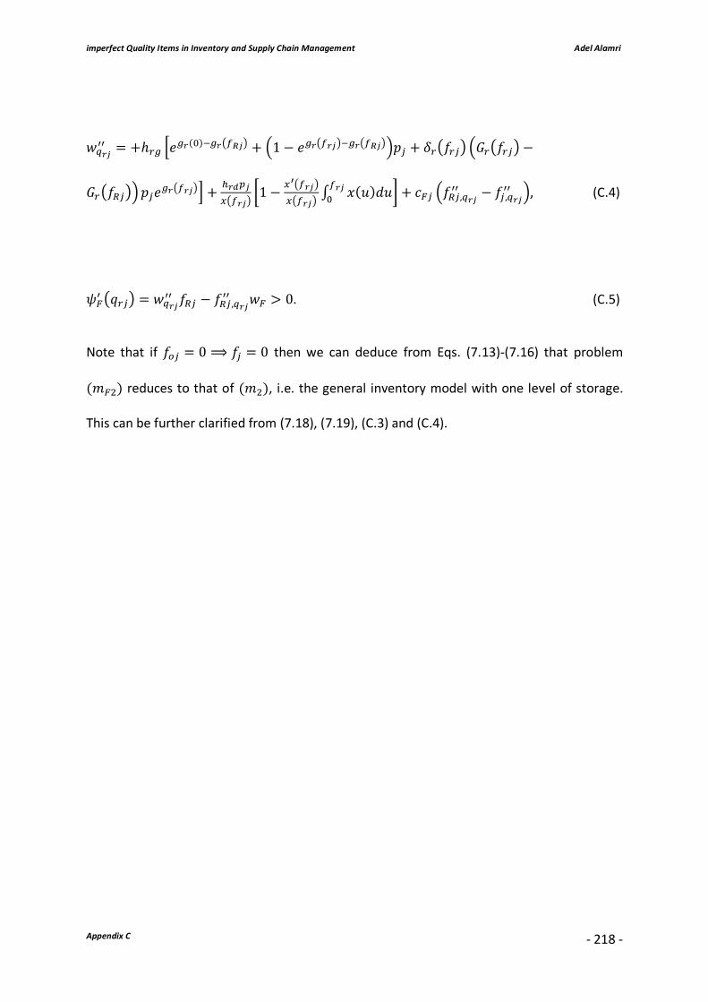
imperfect Quality Items in Inventory and Supply Chain Management Adel Alamri
Appendix C
- 218 -
𝑤ÇÅm�� = +ℎÄ0 z𝑒0Å(q)/0Åe�Omf + A1 − 𝑒0Åe�Åmf/0Åe�OmfG𝑝d + 𝛿Äe𝑓Ädf A𝐺Äe𝑓Ädf −
𝐺Äe𝑓LdfG 𝑝d𝑒0Åe�Åmf{ +�Ås%m�e�Åmf
ë1 − ��e�Åmf�e�Åmf
∫ 𝑥(𝑢)𝑑𝑢�Åmq í + 𝑐Ud A𝑓Ld,ÇÅm
�� − 𝑓d,ÇÅm�� G, (C.4)
𝜓U� e𝑞Ädf = 𝑤ÇÅm�� 𝑓Ld − 𝑓Ld,ÇÅm
�� 𝑤U > 0. (C.5)
Note that if 𝑓Kd = 0 ⟹ 𝑓d = 0 then we can deduce from Eqs. (7.13)-(7.16) that problem
(𝑚Ur) reduces to that of (𝑚r), i.e. the general inventory model with one level of storage.
This can be further clarified from (7.18), (7.19), (C.3) and (C.4).
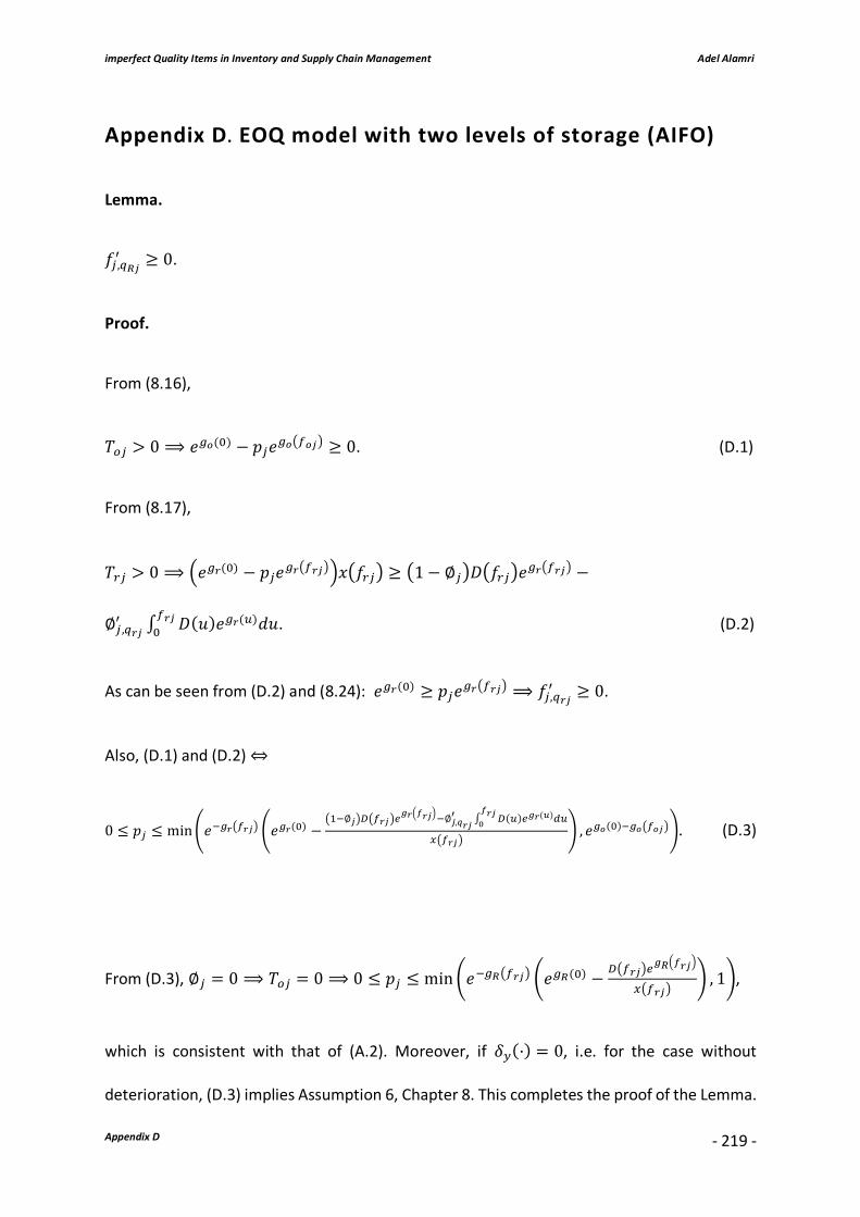
imperfect Quality Items in Inventory and Supply Chain Management Adel Alamri
Appendix D
- 219 -
Appendix D. EOQ model with two levels of storage (AIFO)
Lemma.
𝑓d,ÇOm� ≥ 0.
Proof.
From (8.16),
𝑇Kd > 0 ⟹ 𝑒0N(q) − 𝑝d𝑒0Ne�Nmf ≥ 0. (D.1)
From (8.17),
𝑇Äd > 0 ⟹ A𝑒0Å(q) − 𝑝d𝑒0Åe�ÅmfG𝑥e𝑓Ädf ≥ e1 − ∅df𝐷e𝑓Ädf𝑒0Åe�Åmf −
∅d,ÇÅm� ∫ 𝐷(𝑢)𝑒0Å(v)𝑑𝑢�Åm
q . (D.2)
As can be seen from (D.2) and (8.24): 𝑒0Å(q) ≥ 𝑝d𝑒0Åe�Åmf ⟹ 𝑓d,ÇÅm� ≥ 0.
Also, (D.1) and (D.2) ⇔
0 ≤ 𝑝d ≤ minp𝑒/0Åe�Åmf p𝑒0Å(q) −ej/∅mfæe�Åmf¿
lÅA&ÅmG/∅m,ÈÅm� ∫ æ(v)¿lÅ(])iv
&ÅmÐ
�e�Åmfq , 𝑒0N(q)/0Ne�Nmfq. (D.3)
From (D.3), ∅d = 0 ⟹ 𝑇Kd = 0 ⟹ 0 ≤ 𝑝d ≤ min$𝑒/0Oe�Åmf $𝑒0O(q) − æe�Åmf¿lOA&ÅmG
�e�Åmf' , 1',
which is consistent with that of (A.2). Moreover, if 𝛿×(·) = 0, i.e. for the case without
deterioration, (D.3) implies Assumption 6, Chapter 8. This completes the proof of the Lemma.

imperfect Quality Items in Inventory and Supply Chain Management Adel Alamri
Appendix D
- 220 -
□
The existence, uniqueness and global optimality of the solution can be obtained in a similar
fashion as for the LIFO and FIFO policies, where the conditions under which the global optimal
solution can be attained are given by:
𝑓d,ÇÅm�� =
/Ï∫ æ(v)¿lN(])iv&mÐ Ñ
snÅe�Åmf%m¿
lÅA&ÅmG/W_/lt¸æ
æe�mf¿lÅA&mGPÏ∫ æ(v)¿lN(])iv
&mÐ Ñ
s/u_Q
, (D.4)
∅d,ÇÅm�� =
^r$�m,ÈÅm� æe�mf¿
lNA&mG'w/∫ æ(v)¿lN(])iv
&mÐ $�m,ÈÅm
�� æe�mf¿lNA&mG¸v'`_
Ï∫ æ(v)¿lN(])iv&mÐ Ñ
s , (D.5)
where
𝐴 = 2Ï𝑓d,ÇÅm� 𝐷e𝑓dfÑ
r𝑒A0Ne�mf¸0Åe�mfG ∫ 𝐷(𝑢)𝑒0N(v)𝑑𝑢�m
q ,
𝐵 = A∫ 𝐷(𝑢)𝑒0N(v)𝑑𝑢�mq G
r− 𝑒A0Ne�mf/0Åe�mfG ∫ 𝐷(𝑢)𝑒0N(v)𝑑𝑢�m
q ∫ 𝐷(𝑢)𝑒0Å(v)𝑑𝑢�mq ,
𝐶 = A∫ 𝐷(𝑢)𝑒0N(v)𝑑𝑢�mq G
â− 𝑆 A∫ 𝐷(𝑢)𝑒0N(v)𝑑𝑢�m
q Gr,
𝑋 = 𝑓d,ÇÅm� 𝑒0Åe�mf A𝐷�e𝑓df + 𝛿Äe𝑓df𝐷e𝑓dfG,
𝑌 = 𝑓d,ÇÅm� 𝑒0Ne�mf A𝐷′e𝑓df + 𝛿Ke𝑓df𝐷e𝑓dfG,
𝐷 = 𝑆 Ï2 A𝑓d,ÇÅm� 𝐷e𝑓df𝑒0Ne�mfG
r− 𝑌 ∫ 𝐷(𝑢)𝑒0N(v)𝑑𝑢�m
q Ñ ∫ 𝐷(𝑢)𝑒0Å(v)𝑑𝑢�mq ,

imperfect Quality Items in Inventory and Supply Chain Management Adel Alamri
Appendix D
- 221 -
𝑤ÇÅm�� = +ℎÄ0 z𝑒0Å(q)/0Åe�mf + A1 − 𝑒0Åe�Åmf/0Åe�mfG𝑝d + 𝛿Äe𝑓Ädf A𝐺Äe𝑓Ädf −
𝐺Äe𝑓dfG𝑝d𝑒0Åe�Åmf + ∅d,ÇÅm�� A𝐺Äe𝑓df ∫ 𝐷(𝑢)𝑒0Å(v)𝑑𝑢�m
q − ∫ 𝐷(𝑢)𝐺Ä(𝑢)𝑒0Å(v)𝑑𝑢�mq G +
∅d,ÇÅm� 𝑒/0Åe�mf ∫ 𝐷(𝑢)𝑒0Å(v)𝑑𝑢�m
q { + �Ås%m�e�Åmf
ë1 − ��e�Åmf�e�Åmf
∫ 𝑥(𝑢)𝑑𝑢�Åmq í +
ℎK0 z∅d,ÇÅm�� ∫ 𝐷(𝑢)𝐺K(𝑢)𝑒0N(v)𝑑𝑢
�mq + A∅d,ÇÅm
�� + 2∅d,ÇÅm� G 𝑓d,ÇÅm
� 𝐷e𝑓df𝐺Ke𝑓df𝑒0Ne�mf{, (D.6)
𝜓W� e𝑞Ädf = 𝑤ÇÅm�� 𝑓d − 𝑓d,ÇÅm
�� 𝑤W > 0. (D.7)
Note that 𝛿Ä(·) = 𝛿K(·) ⟹ (8.23) ⇔ 𝑓d,ÇÅm� = ¿lÅ(Ð)/%m¿
lÅA&ÅmG
æe�mf¿lÅA&mG
⟹ (D. 4)
⇔ 𝑓d,ÇÅm�� =
/%mnÅe�Åmf¿lÅA&ÅmG/�m,ÈÅm
� Aæ�e�mf¸nÅe�mfæe�mfG¿lÅA&mG
æe�mf¿lÅA&mG
.
Considering the above and (8.21), (8.25) and (D.6), ∅d = 0 ⟹ 𝑇Kd = 0, the model reduces to
that of of (𝑚r), i.e. the general inventory system with one level of storage.