impact of the panama canal expansion in global …
TRANSCRIPT
IMPACT OF THE PANAMA CANAL EXPANSION IN GLOBAL SUPPLY CHAIN:
OPTIMIZATION MODEL FOR US CONTAINER SHIPMENT
A Dissertation
Submitted to the Graduate Faculty
of the
North Dakota State University
of Agriculture and Applied Science
By
Ju Dong Park
In Partial Fulfillment of the Requirements
for the Degree of
DOCTOR OF PHILOSOPHY
Major Program:
Transportation and Logistics
March 2015
Fargo, North Dakota

North Dakota State University
Graduate School
Title
IMPACT OF THE PANAMA CANAL EXPANSION IN GLOBAL SUPPLY
CHAIN: OPTIMIZATION MODEL FOR THE U.S. CONTAINER SHIPMENT
By
Ju Dong Park
The Supervisory Committee certifies that this disquisition complies with North Dakota State
University’s regulations and meets the accepted standards for the degree of
DOCTOR OF PHILOSOPHY
SUPERVISORY COMMITTEE:
Dr. Won W. Koo
Chair
Dr. Joseph Szmerekovsky
Dr. Saleem Shaik
Dr. Seung Won Hyun
Approved:
3-30-2015 Dr. Denver Tolliver
Date Department Chair
iii
ABSTRACT
The transportation of containerized shipments will continue to be a topic of interest in the
world because it is the primary method for shipping cargo globally. The primary objective of this
study is to analyze the impact of the Panama Canal Expansion (PCE) on the trade flows of
containerized shipments between the United States and its trade partners for US exports and
imports. The results show that the Panama Canal Expansion would affect the trade flows of US
imports and exports significantly. The major findings are as follows: (1) the PCE affects not only
US domestic trade flows, but also international trade flows since inland transportation and ocean
transportation are interactive, (2) delay cost and toll rate at the Panama Canal do not have a
significant impact on trade volume and flows of US containerized shipments after the Panama
Canal Expansion mainly because delay cost and toll rate at the canal account for a small portion
of the total transportation costs after the PCE, (3) West Coast ports would experience negative
effects and East Coast ports would experience positive effects from the PCE, while Gulf ports
would experience no effects from the PCE, and (4) an optimal toll rate is inconclusive in this
study because changes in toll rate at the canal account for a small portion of the total
transportation costs and the PNC competes with shipments to/from Asia shipping to the US West.

iv
ACKNOWLEDGMENTS
I would like to gratefully and sincerely thank Dr. Won W. Koo for his guidance,
understanding, patience, and most importantly, his mentorship during my graduate studies at
North Dakota State University. His mentorship was paramount in providing a well-rounded
experience consistent with my career goals. I wish I had satisfied his expectation as the last
student in his academic life. For everything you have done for me, Dr. Koo, I truly thank you. I
would also like to thank my committee members: Dr. Joseph Szmerekovsky, whose comments
improved supply chain issues in the dissertation: Dr. Saleem Shaik, who shared solid knowledge
of operation research and individual suggestions regarding research methodology:, and Dr.
Seung Won Hyun, who was always willing to help and give his best suggestions and
encouragement. The help they have given me during graduate school and a successful career at
North Dakota State University is greatly appreciated. Special appreciation goes to Richard
Taylor for all his help and advice in developing the GAMS code for my dissertation. I am
especially grateful to the director of the Upper Great Plains Transportation Institute, Dr. Denver
Tolliver, whose great support improved my academic career. I would like thank the staff at
UGPTI, especially Jody Bohn, Dr. Dybing and Doug Benson. In addition, I would like to thank
Dr. Chiwon Lee, Dr. Sang Young Moon, Dr. Junwook Chi, and Dr. Eunsu Lee. Thanks to Poyraz
Kayabas, Wonjoo Cho, Yongshin Park, Juho Choi, Haram Kim, and Jaesung Choi for their
friendship in Fargo, North Dakota. Finally, and most importantly, I would like to thank my
parents, Panyeop Park and Namsun Kang, for their faith in me and allowing me to be as
ambitious as I wanted. I want thank my two order sisters (Seohee Park and Younghee Park), two
brothers-in-law (Ohmin Kwon and Taeho Hwang) and my lovely niece (Jeonghyun Hwang) and
nephew (Juhyun Hwang). Their support, encouragement, quiet patience and unwavering love

v
were undeniably the bedrock upon which the past 10 years of my life in the United States have
been built. Especially, all my honor goes to my dad, who is at rest since last May.

vi
TABLE OF CONTENTS
ABSTRACT ................................................................................................................................. iii
ACKNOWLEDGMENTS ........................................................................................................... iv
LIST OF TABLES ....................................................................................................................... ix
LIST OF FIGURES ....................................................................................................................... x
LIST OF APPENDIX TABLES ................................................................................................. xii
LIST OF APPENDIX FIGURES ............................................................................................... xiii
CHAPTER 1. INTRODUCTION ................................................................................................. 1
1.1. Background of Problem Statement ............................................................................. 1
1.2. Statements of the Problem ........................................................................................ 10
1.3. Research Objective ................................................................................................... 12
1.4. Assumptions .............................................................................................................. 14
1.5. Organization .............................................................................................................. 15
CHAPTER 2. LITERATURE REVIEW .................................................................................... 17
2.1. Spatial Optimization Models .................................................................................... 17
2.2. Transportation Costs and Container Shipment Trade ............................................... 19
2.3. Operation of the Current Panama Canal and Its Expansion ..................................... 23
CHAPTER 3. MODEL DEVELOPMENT ................................................................................. 28
3.1. Theoretical Foundation ............................................................................................. 28
3.2. Basic Structure of Container Shipment Model ......................................................... 31
3.3. Model Description .................................................................................................... 33
3.4. Spatial Optimization Model for US Exports ............................................................. 35
3.5. Spatial Optimization Model for US Imports ............................................................. 40

vii
3.6. Spatial Optimization Model for US Container Trade ............................................... 46
CHAPTER 4. DATA COLLECTION ........................................................................................ 50
4.1. Supply and Demand .................................................................................................. 50
4.1.1. US Exports ................................................................................................. 50
4.1.2. US Imports ................................................................................................. 51
4.2. Shipping Origins and Destinations ........................................................................... 51
4.3. Transportation Costs ................................................................................................. 52
4.3.1. Ocean Transportation Costs ....................................................................... 52
4.3.2. Barge Transportation Costs ........................................................................ 53
4.3.3. Rail Transportation Costs .......................................................................... 54
4.3.4. Truck Transportation Costs ........................................................................ 55
4.3.5. Summary .................................................................................................... 55
4.4. Cargo Handling Charges at Container Ports ............................................................. 56
4.5. Delay Costs and Toll Rates at the Panama Canal ..................................................... 56
4.6. Cargo Handling Capacity of US Ports and the Panama Canal ................................. 57
CHAPTER 5. EMPIRICAL RESULTS ..................................................................................... 58
5.1. Spatial Optimization under the Base Model vs. the Panama Canal and the
US Port Expansion ................................................................................................... 58
5.1.1. Trade Volume of Containerized Shipments for US Exports ..................... 60
5.1.2. Trade Volume of Containerized Shipments for US Imports ..................... 65
5.1.3. Trade Volume and Total Toll Revenue of Containerized Shipments
at the Panama Canal .................................................................................. 70
5.1.4. Trade Volume and Flows at Container Ports in the United States ............ 72
5.1.5. Domestic Trade Volume and Flows of Containerized Shipments
in the United States .................................................................................... 77
viii
5.1.6. Impacts of the Panama Canal Expansion on the competitiveness
of intermodal and intramodal systems in the United States ...................... 89
5.1.7. International Trade Volume and Flows of Containerized Shipments
in the United States .................................................................................... 98
5.1.8. Summary .................................................................................................. 106
5.2. Impacts of Changes in Toll Rates at the Panama Canal ......................................... 108
5.2.1. Changes in Trade Volume of Containerized Shipments Transited
through the Panama Canal ....................................................................... 108
5.2.2. Economic Value of the Panama Canal Expansion ....................................112
5.2.3. Summary .................................................................................................. 115
CHAPTER 6. SUMMARY AND CONCLUSIONS ................................................................ 118
REFERENCES .......................................................................................................................... 122
APPENDIX A. EXPORT DEMAND AND IMPORT SUPPLY FOR US
EXPORTS (TEUs) ......................................................................................... 127
APPENDIX B. EXPORT DEMAND AND IMPORT SUPPLY FOR US IMPORTS
(TEUs) ............................................................................................................. 130
APPENDIX C. CARGE HANDLING COSTS (US$) AT PORTS IN EXPORTING
AND IMPORTING COUNTRIES ................................................................. 134
APPENDIX D. CARGO HANDLING CAPACITIES OF THE PANAMA CANAL
AND US PORTS (TEUs) ............................................................................... 136
APPENDIX E. INLAND TRANSPORTATION NETWORKS IN THE UNITED
STATES .......................................................................................................... 137
APPENDIX F. OCEAN TRANSPORTATION NETWORKS IN THE UNITED
STATES .......................................................................................................... 139
APPENDIX G. QUANTITIES OF EXPORTS AND IMPORTS IN 49 STATES OF US
MAINLAND (TEUs) ...................................................................................... 141
APPENDIX H. Q&A FROM PERSONAL INTERVIEW ...................................................... 143
APPENDIX I. GAMS CODE ................................................................................................. 144
ix
LIST OF TABLES
Table Page
5.1. An average of actual trade volume between US shipping origins and its 15
trade partners from 2011 to 2013 (TEUs) ........................................................................ 62
5.2. An average of actual trade volume between US shipping destinations and its
15 trade partners from 2011 to 2013 (TEUs) ................................................................... 67
5.3. Trade volume and the total toll revenue of containerized shipments at the
Panama Canal ................................................................................................................... 71
5.4. Trade volume and flows at container ports in the United States ...................................... 73
5.5. Domestic trade volume and flows of containerized shipments by truck in the
United States (TEUs) ....................................................................................................... 78
5.6. Domestic trade volume and flows of containerized shipments by truck-barge
combination in the United States (TEUs) ........................................................................ 81
5.7. Domestic trade volume and flows of containerized shipments by rail in the
United States (TEUs) ....................................................................................................... 84
5.8. Shares of domestic transportation modes in the United States ........................................ 90
5.9. Optimal choices of US domestic transportation mode in changes of
international trade circumstance ...................................................................................... 97
5.10. Shares and changes of international trade volume of containerized shipments
in the United States ........................................................................................................ 104
5.11. Changes in trade volume of containerized shipments at the Panama Canal by
the PNC toll changes ...................................................................................................... 109
5.12. Changes in the total toll revenue at the Panama Canal by the PNC toll changes .......... 113

x
LIST OF FIGURES
Figure Page
1.1. World container traffic and throughput (millions of TEU) (Drewry Shipping
Consultants, 2014) ............................................................................................................. 2
1.2. Global exports and container throughput (WTO and Drewry Shipping
Consultants, 2013) ............................................................................................................. 3
1.3. Top 15 trading partners for US containerized exports (US Maritime
Administration, 2013) ........................................................................................................ 4
1.4. Top 15 trading partners for US containerized imports (US Maritime
Administration, 2013) ........................................................................................................ 5
1.5. Container export trends at US coasts (US Maritime Administration, 2012) ..................... 6
1.6. Container import trends at US coasts (US Maritime Administration, 2012) ..................... 7
1.7. Shares of container flows between Northeast Asia and US East Coast ports
(Panama Canal Authority, 2010) ....................................................................................... 8
1.8. General Information of the New Locks at PNC (Panama Canal Authority, 2012) ......... 10
3.1. Effects of Transportation Cost (Koo, 1984) .................................................................... 29
3.2. Relationship between trade volume and toll rate at the Panama Canal ........................... 30
3.3. Hypothetical trip cost curves for rail (RR’), truck (TT’), and barge (WW’) modes
of transportation for a given origin/destination (Koo, Tolliver, and Bitzan, 1993) ......... 32
3.4. Classification of container vessel by its capacity (in meters) (Ashar and
Rodrigue, 2012) ............................................................................................................... 33
3.5. Regions associated with container trade and transportation modes for
US exports ........................................................................................................................ 36
3.6. Regions associated with container trade and transportation modes for
US imports ....................................................................................................................... 41
5.1. Official regions of the United States. Source: US Census (2015) ................................... 65
5.2. Distribution of domestic transportation modes prior to the Panama Canal
Expansion in the United States ........................................................................................ 91
xi
5.3. Distribution of domestic transportation modes after the Panama Canal
Expansion in the United States ........................................................................................ 93
5.4. Distribution of domestic transportation modes after the Panama Canal and
US port expansion in the United States ........................................................................... 96
5.5. Ocean trade flows of containerized shipments in the United States ................................ 99
5.6. Ocean trade flows of containerized shipments after the Panama Canal
Expansion in the United States ...................................................................................... 101
5.7. Ocean trade flows of containerized shipments after the Panama Canal and
US port expansion in the United States ......................................................................... 102
5.8. Total trade volume of containerized shipments by coastal regions in
the United States ............................................................................................................ 106
5.9. Total volume and toll revenue in changes of toll rate at the Panama Canal .................. 117

xii
LIST OF APPENDIX TABLES
Table Page
A1. Export Demand and Import Supply for US Exports (TEUs) ......................................... 128
B1. Export Demand and Import Supply for US Imports (TEUs) ......................................... 131
C1. Cargo Handling Costs (US$) at Ports in Exporting and Importing Countries ............... 135
D1. Cargo Handling Capacities of the Panama Canal and US Ports (TEUs) ....................... 136

xiii
LIST OF APPENDIX FIGURES
Figure Page
E1. Inland Transportation Networks in the United States .................................................... 138
F1. Ocean Transportation Networks in the United States .................................................... 140
G1. Quantities of Exports and Imports in 49 States of US Mainland (TEUs) ...................... 142
1
CHAPTER 1. INTRODUCTION
1.1. Background of Problem Statement
The container shipping industry plays an important role in the transportation of freight.
Between 1990 and 2008, containerization began to seriously impact global trade patterns. During
the same period, a new class of Panamax containerships became a dominant vector of maritime
shipping. Figure 1.1 shows the growth of world container traffic and throughput, full/empty
containers, and transshipments from 1980 to 2013. The world container traffic was increased
continuously from 28.7 million TEUs (twenty-foot equivalent units) in 1990 to 152.0 million
TEUs in 2008, an increase of about 530%. This corresponds to an average annual compound
growth of 9.5%. During the same period, container throughput, which includes TEUs at the port
of origin, destination and transshipment, grew from 88 million to 530 million TEUs, an increase
of 600%, equivalent to an average annual compound growth of 10.5%. The trend underlines a
divergence between throughput and traffic as global supply chains became more complex.
Consequently, the ratio of container traffic over container throughput was around 3.5 in 2008,
whereas this ratio was 3.0 in 1990. However, the financial crisis of 2009-2010 had a significant
impact on container flows, which experienced a drop of 49 million TEUs (9.3%) between 2008
and 2009 (WTO, 2013).

2
Figure 1.1. World container traffic and throughput (millions of TEU) (Drewry Shipping
Consultants, 2014).
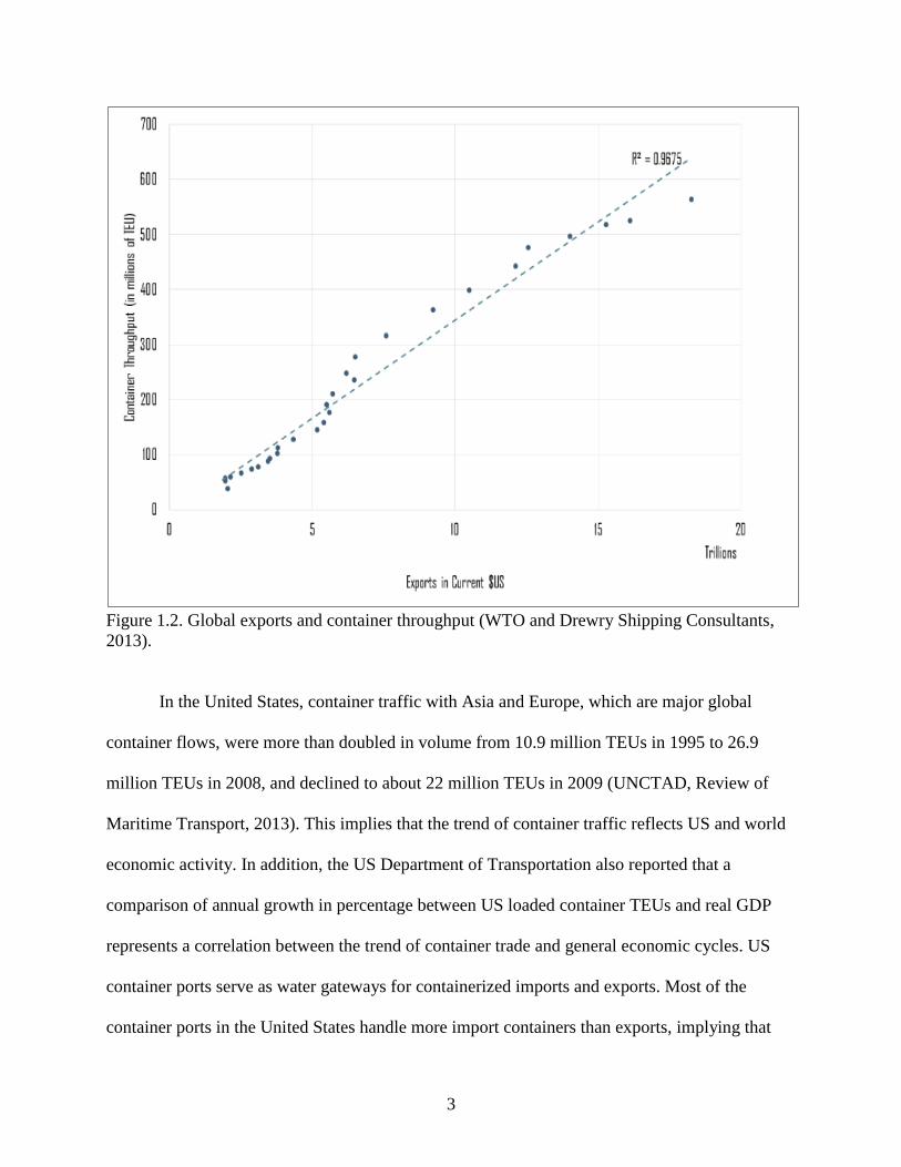
Figure 1.2 shows a correlation between global exports and global container throughput
from 1980 to 2010 with 𝑅2 of 0.97. Although this relation is proportional, Figure 1.2 shows that
there is a direct relationship between the volume of world container throughput (TEU) and global
exports as the number (TEU) of world container throughput increased when global exports
increased during the same period. This implies that the trend of container traffic reflects world
economic activity.
3
Figure 1.2. Global exports and container throughput (WTO and Drewry Shipping Consultants,
2013).
In the United States, container traffic with Asia and Europe, which are major global
container flows, were more than doubled in volume from 10.9 million TEUs in 1995 to 26.9
million TEUs in 2008, and declined to about 22 million TEUs in 2009 (UNCTAD, Review of
Maritime Transport, 2013). This implies that the trend of container traffic reflects US and world
economic activity. In addition, the US Department of Transportation also reported that a
comparison of annual growth in percentage between US loaded container TEUs and real GDP
represents a correlation between the trend of container trade and general economic cycles. US
container ports serve as water gateways for containerized imports and exports. Most of the
container ports in the United States handle more import containers than exports, implying that
4
the US has been facing a trade deficit in container shipments. About 60% of the international
container trade is for imports and more than 80% of import containers are handled by US major
container ports in 2012. However, most currently, US waterborne container export is 11.9
million TEUs in 2012, a 4% increase from the 10.7 million TEUs in 2007 (US Maritime
Administration, 2013).
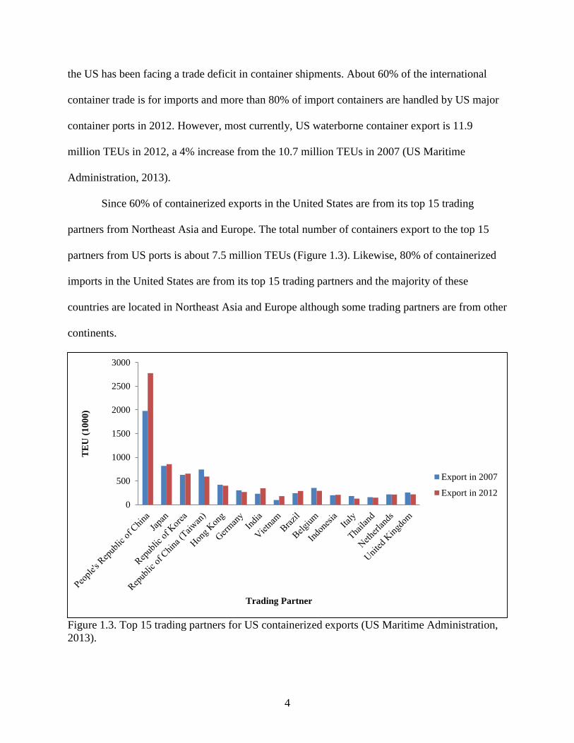
Since 60% of containerized exports in the United States are from its top 15 trading
partners from Northeast Asia and Europe. The total number of containers export to the top 15
partners from US ports is about 7.5 million TEUs (Figure 1.3). Likewise, 80% of containerized
imports in the United States are from its top 15 trading partners and the majority of these
countries are located in Northeast Asia and Europe although some trading partners are from other
continents.
Figure 1.3. Top 15 trading partners for US containerized exports (US Maritime Administration,
2013).
0
500
1000
1500
2000
2500
3000
TE
U (
10
00
)
Trading Partner
Export in 2007
Export in 2012

5
Figure 1.4. Top 15 trading partners for US containerized imports (US Maritime Administration,
2013).
Containerized imports to all US ports from these top 15 trade partners is about 13.9
million TEUs which is about 80% of the total imports in the United States (Figure 1.4). The
People’s Republic of China (hereafter, China) is the biggest trade partner for containerized
shipments in the United States, since more than 35% of container shipments, among these top 15
exporters, is exported to China from the US and 60% of container shipments, among these top 15
importers, is imported from China to the US. Trade volume between the US and China is
overwhelmingly larger than trade volume between the US and other countries.
Figure 1.5 shows export trends of container shipments at different US coasts. Between
2008 and 2009, exports of container shipments at US West Coast ports decreased by 0.3 million
TEUs, exports of container shipments at US East Coast ports decreased by 0.5 million TEUs, and
exports of container shipments at US Gulf Coast ports remained about same. On the other hand,
between 2008 and 2012, exports of container shipments from both the US West Coast ports and
0
1000
2000
3000
4000
5000
6000
7000
8000
9000
10000T
EU
(1
00
0)
Trading Partner
Import in 2007
Import in 2012

6
East Coast ports increased by 0.3 million TEUs, whereas exports of container shipments from
US Gulf Coast ports increased by 0.1 million TEUs.
Figure 1.5. Container export trends at US coasts (US Maritime Administration, 2012).
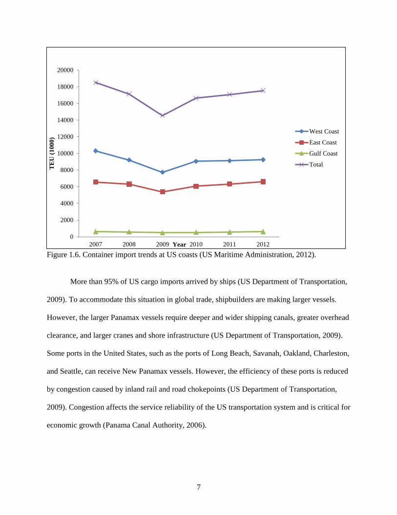
Figure 1.6 represents that import trends of container shipments at different US coasts.
Between 2007 and 2009, imports of container shipments at the US West Coast ports decreased
by 2.6 million TEUs. Imports of container shipments at US East Coast ports decreased by 1.2
million TEUs, whereas imports of container shipments at US Gulf Coast ports decreased by 0.1
million TEUs. However, from 2009 to 2012, imports of container shipments at US West Coast
ports increased by 1.5 million TEUs, increased by 1.2 million TEUs at US East Coast ports, and
also increased by 0.1 million TEUs at US Gulf Coast ports. As a result, trades of container
shipments at US West Coast ports decreased 1.1 million TEUs, while trades of container
shipments at US East Coast and Gulf Coast ports remained about same from 2007 to 2012
0
2,000
4,000
6,000
8,000
10,000
12,000
14,000
2007 2008 2009 2010 2011 2012
TE
U (
10
00
)
Year
West Coast
East Coast
Gulf Coast
Total
7
Figure 1.6. Container import trends at US coasts (US Maritime Administration, 2012).
More than 95% of US cargo imports arrived by ships (US Department of Transportation,
2009). To accommodate this situation in global trade, shipbuilders are making larger vessels.
However, the larger Panamax vessels require deeper and wider shipping canals, greater overhead
clearance, and larger cranes and shore infrastructure (US Department of Transportation, 2009).
Some ports in the United States, such as the ports of Long Beach, Savanah, Oakland, Charleston,
and Seattle, can receive New Panamax vessels. However, the efficiency of these ports is reduced
by congestion caused by inland rail and road chokepoints (US Department of Transportation,
2009). Congestion affects the service reliability of the US transportation system and is critical for
economic growth (Panama Canal Authority, 2006).
0
2000
4000
6000
8000
10000
12000
14000
16000
18000
20000
2007 2008 2009 2010 2011 2012
TE
U (
10
00
)
Year
West Coast
East Coast
Gulf Coast
Total
8
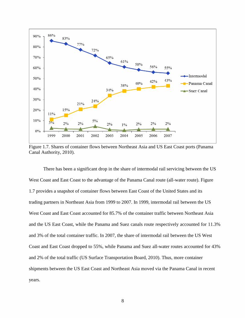
Figure 1.7. Shares of container flows between Northeast Asia and US East Coast ports (Panama
Canal Authority, 2010).
There has been a significant drop in the share of intermodal rail servicing between the US
West Coast and East Coast to the advantage of the Panama Canal route (all-water route). Figure
1.7 provides a snapshot of container flows between East Coast of the United States and its
trading partners in Northeast Asia from 1999 to 2007. In 1999, intermodal rail between the US
West Coast and East Coast accounted for 85.7% of the container traffic between Northeast Asia
and the US East Coast, while the Panama and Suez canals route respectively accounted for 11.3%
and 3% of the total container traffic. In 2007, the share of intermodal rail between the US West
Coast and East Coast dropped to 55%, while Panama and Suez all-water routes accounted for 43%
and 2% of the total traffic (US Surface Transportation Board, 2010). Thus, more container
shipments between the US East Coast and Northeast Asia moved via the Panama Canal in recent
years.

9
More than 1 million vessels have transited through the Panama Canal since it opened in
1914. The Panama Canal has served as a pathway for major world commodities and the
importance of the Panama Canal continues to grow due to increases in trade between the United
States and Asia. Container shipments have become the major type of commodities through the
canal, although bulk shipments used to be major commodities through the canal in its history.
Now the canal is under the construction to expend the existing canal system. The Panama
Canal is an efficient route between the US Gulf /East Coasts and Northeast Asia, but is reaching
its maximum capacity. However, this problem would be resolved in 2016 when the Panama
Canal expansion project is completed. Most currently, the Panama Canal Authority reported 86%
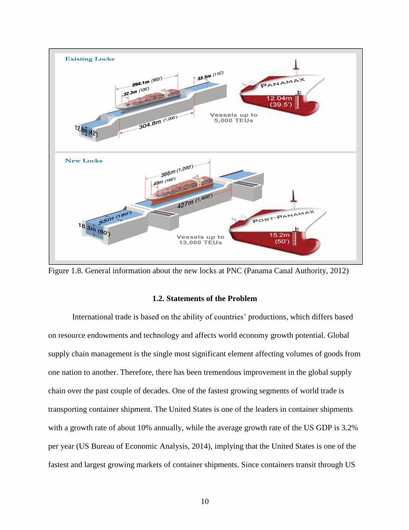
of the expansion project was completed on February 2015. Figure 1.8 shows details of the
existing locks and the new locks being built at the Panama Canal. As shown in Figure 1.8, major
parts of the expansion project include dredging and the building of new locks. Dredging is the
largest part of the expansion project since it will be able to allow New Panamax vessels to move
through the Canal. The locks will be 38 feet wider, 18 feet deeper, and 401 feet longer than the
current locks (Panama Canal Autuhority, 2012). The new locks will allow New Panamax vessels
to move through the Canal. Since New Panamax vessels carry 12,500 TEUs of container
shipments, while current Panamax vessels carry only 4,500 TEUs of container shipments, the
expansion project will lead to more than a doubled capacity of the Canal. Therefore, the
expansion project will accommodate growing trade volumes of container shipments and reduce
congestion.
10
Figure 1.8. General information about the new locks at PNC (Panama Canal Authority, 2012)
1.2. Statements of the Problem
International trade is based on the ability of countries’ productions, which differs based
on resource endowments and technology and affects world economy growth potential. Global
supply chain management is the single most significant element affecting volumes of goods from
one nation to another. Therefore, there has been tremendous improvement in the global supply
chain over the past couple of decades. One of the fastest growing segments of world trade is
transporting container shipment. The United States is one of the leaders in container shipments
with a growth rate of about 10% annually, while the average growth rate of the US GDP is 3.2%
per year (US Bureau of Economic Analysis, 2014), implying that the United States is one of the
fastest and largest growing markets of container shipments. Since containers transit through US
11
seaports, container shipments have a significant impact on seaports, as well as intermodal
transportation networks between the ports and inland.
Transportation costs of shipping containerized cargo from shipping origins in exporting
countries to shipping destinations in importing countries consist of ocean transportation costs,
inland transportation costs, cargo handling charges for loading and unloading at ports in
exporting and importing countries, tolls at the canal (if the shipping route includes the canal),
and delay costs (at the canal). Domestic transportation in an exporting country and international
transportation cannot be separated and examined individually because they are interdependent.
There are interactions between domestic and international transportation. Domestic
transportation costs affect international trade flows, as well as domestic trade flows in an
exporting country. Inland transportation systems in exporting countries are another concern.
How effectively inland transportation systems deliver containerized cargo from shipping origins
to the export ports in exporting countries may be a critical measurement of countries’
competitiveness in the world trade of container shipments.
The US railroad industry experiences intramodal and intermodal competition. Intramodal
competition among railroad operators stimulates efficiency of rail transportation and reduces
freight rates. Since railroads compete with barges in shipping containerized cargo from shipping
origins to the US Gulf Coast ports, intermodal competition between rail and barge transportation
also plays an important role in reducing rail freight rates. While the rail industry increases its
efficiency to compete with barges, the barge industry loses its efficiency by decrepitude and
erosion of dams and locks on river systems.
Global economics is driving the use of large vessels with their economies of scale. Ports
that can handle these large vessels are expected to increase their market shares. Container traffic
12
in the United States tends to be highly concentrated and is becoming even more so as larger
vessels call on ports that are capable of handling them. As a result of these concentrations,
increases in container shipping capacity (particularly enroute between Northeast Asia and the
United States), and the escalation in vessel sizes, substantial strain or perception of future strain
on capacity at most US ports is felt as well as in associated transportation corridors.
Changes in ocean transportation costs; toll, and delay costs at the Panama Canal; and port
capacity after the PCE in exporting and importing countries are the most significant factors
determining world container trade flows. A change in these factors is favorable to some
exporting and importing countries, but not favorable to all. It is also necessary to evaluate how
the changes in these factors affect the world trade of container shipments and individual
exporting and importing countries.
The Panama Canal Expansion (PCE) may positively affect container shipment trade in
the United States since the canal is a gateway for transporting containerized cargo between the
United States and Asia. By completion of the expansion, transportable vessel size through the
canal will increase from current Panamax size (4,500 TEUs) to a new Panamax size (12,500
TEUs) and efficiency of canal operation and its operation costs would increase. As a result, toll
rates may be increased by the Panama Canal Authority, which has rights for operations and
maintenance, to maximize its revenue from the canal.
1.3. Research Objective
The main objective of this study is to analyze the impacts of the Panama Canal
Expansion (PCE) on the flows of containerized shipments from shipping origins in the United
States to its export destinations and its impact on flows of containerized cargo from ports in
exporting countries to shipping destinations in the US, with special interest in the flows of
13
container shipments between the United States and Northeast Asia and Europe. More specifically,
the study is designed to examine the following scenarios: (1) investigate the impacts of PCE on
the transportation costs of US container shipments, (2) evaluate the impacts of the PCE on the
trade volume and flows of container shipments through analyzing US container shipments
comparing pre-PCE to after, (3) investigate impacts of delay cost at the PNC on the trade volume
and flows of containerized shipments for US exports and imports, (4) examine the impacts of
alternative toll rates in the Panama Canal on the flows of container shipments to ports in the
United States and ocean shipping routes, (5) estimate an optimal toll rate to maximize the
Panama Canal’s revenue after PCE, (6) estimate throughput of container shipments at the
Panama Canal after PCE, and (7) estimate port handling capacity in the United States after PCE.
The primary focus of this research is US trade of container shipments with Northeast
Asia and Europe. Since Northeast Asia has a large trade volume of container shipments, the area
of interest is whether more US container shipments will be shipped through the US Gulf and East
Coast ports via the Panama Canal or if US container shipments will be shipped through US West
Coast ports such as the Pacific Northwest (PNW) or Los Angeles/Long Beach (LA/LB). The
major contributions of this study are that it evaluates impacts of toll rates at the Panama Canal
due to the expansion of container trade flows, it estimates the economic value of the canal
expansion in the world container trade, and estimates further needs of ocean and inland
transportation infrastructures.
14
1.4. Assumptions
The model developed for this study is based on the following assumptions.
(1) The values of containerized cargo are ignored, mainly because the container is
the equipment used for the shipping of commodities/products between
shipping origin and destination.
(2) It is assumed that every container is fully loaded, while its total weight is 24
tons with 22 tons of net load. In this general situation, for normal or low value
cargo, most shippers and carriers would not leave any wasted space inside
containers because most ocean carriers (liners) charge shipping costs based on
TEU rather than tonnage for containerized shipments. Although shipping rates
are differentiated by container type, such as frozen, empty, and loaded, it does
not charge based on cargo weight.
(3) US containerized shipments are moved by rail, truck, and barge between
shipping origins/destinations. Trucks transit containerized shipments within
less than 250 miles between shipping origins/destinations, and rail is used for
distances greater than 250 miles. Truck and barge combinations are also used
on the U.S. river systems.
(4) From the 1990s to 2000s, barge liners operated their services to transit
containerized shipments between the Gulf ports and river ports along the US
river systems because there were enough shipments for liner services and it
was competitive with rail operations for long hauling. However, many barge
liners quit operating their services for containers mainly because of the
backhaul shortage at the end of 2000s. In other words, they had enough

15
shipments from the Gulf ports to river ports along the river systems for US
imports, but there were not enough shipments on a return trip from river ports
to the Gulf ports. This implies that the United States is a trade deficit country.
In the United States, only one barge carrier still transports containers on barge
service now and their service is based on contract rather than line service
(Koenning, 2014). Therefore, it is assumed that container service is available
at all river ports with their unlimited port capacities in the United States for
barge service.
1.5. Organization
The introduction to the study, a background, the importance of container shipment trade,
statement of the problem and objectives, and major assumptions were outlined previously. The
remainder of this dissertation is organized as follows. Chapter 2 presents an extensive review of
relevant literature on linear programing models, transportation cost models, container activity,
and the Panama Canal expansion. The foundation of the study and insights on theory and
methodology were built up through review of similar studies in this chapter. Chapter 3 outlines
the theoretical foundation and background for model development and structure. The
deterministic of base optimization model is developed. The major model parameter estimation
and assumptions are explored in this chapter.
Data collection for this study is represented in Chapter 4. Chapter 4 describes details and
procedures of data collection and development for supply and demand, transportation cost
estimation, and the PNC delay cost. Chapter 5 presents the results found in regards to the trade
flows and transportation costs associated with US containerized shipments under the base and
alternative models. The results are also used to comparatively analyze the impacts of the Panama

16
Canal Expansion (PCE) on US trade. Chapter 6 summarizes and concludes and provides overall
major findings and contributions for this dissertation. Finally, nine appendixes are included.
Appendix A shows export demand and import supply (TEUs) for US exports. Appendix B
presents export demand and import supply (TEUs) for US imports. Appendix C represents cargo
handling costs (US$) at ports in exporting and importing countries. Appendix D shows cargo
handling capacities of the Panama Canal and US container ports (TEUs). Appendix E represents
inland transportation networks used for this study. Appendix F shows ocean transportation
networks used for this study. Appendix G represents the quantities of exports and imports in the
49 states of the US mainland (TEUs). Appendix H shows Q&A during a personal interview with
an expert in the barge industry in a phone interview. Appendix I shows GAMS code for the base
model of this study.

17
CHAPTER 2. LITERATURE REVIEW
The study of the use of container shipments has been active, especially during recent
decades of global booming trade. There exists a large body of research on spatial optimization
modeling, spatial equilibrium modeling, transportation cost modeling, traffic flow optimization,
infrastructure planning, intermodal simulation, empty container allocation problem, ocean ship
scheduling, freight security, and freight network modeling. This chapter reviews current and
previous research on the container shipping industry. The review covers literatures ranging from
general research on global container trade, to supply chain network planning, to relevant
mathematic methodology.
2.1. Spatial Optimization Models
Koo and Thompson (1982) developed a spatial optimization model using a linear
programming algorithm to optimize US grain distribution systems. The objective function of this
model is to minimize transportation and handling costs associated with transportation activities
for the US grain trade. The authors found that the capacity constraints of transportation modes
determine the flow of grain from shipping origins to destinations. The capacity constraints of
transportation modes do not affect the flow when using shorter shipping distances and changes in
grain flow to domestic markets. On the other hand, changes in costs of transportation modes
affect intermodal transportation systems from origins to destinations since demand for barge
service has more price elasticity than for rail services.
Koo, et al. (1988) used a spatial optimization model to optimize domestic and
international grain flows. The authors found that international grain flow is influenced more by
changes in ocean transportation costs at a particular port rather than by uniform changes at all
ports. The reallocation of export shipments from the Gulf to other ports results in high freight

18
rates for several importing regions because domestic transportation costs from major shipping
origins are lower to US Gulf ports than to other US ports. The cheapest transportation mode for
long distance transport to US Gulf ports is barge along the Mississippi River system. In addition,
once ocean transportation costs from the Gulf ports to East Asia increase, quantities of grain
shipped from the US West Coast to East Asia substantially increase.
Wilson, Koo, Taylor, and Dahl (2005) developed a large-scale spatial optimization model
based on a longer-term competitive equilibrium to make projections in the world grain trade. The
spatial distribution of grain flows are affected by changes in world grain trade. The changes in
world grain trade are influenced by many factors, including production, consumption (which is
impacted by tastes, population and income growth), and agricultural and trade policies. In
addition, relative costs of production, interior shipping, handling and ocean transportation costs
all have an impact on trade and competitiveness. Six major grains (wheat, corn, soybean, barley,
sorghum, and rice) were identified for this study and very detailed data was generated.
According to this study, world trade should increase by about 47%, with the fastest growth
occurring in imports to China and Pakistan. Japan and the European Union (EU), traditionally
large markets, are expected to have the slowest growth. Most of the increases are expected in
soybeans (49%), followed by corn (26%), and most of US exports growth is expected through
the US Gulf.
Wilson, Koo, Taylor, and Dahl (2005) developed a detailed spatial optimization model of
the world grain trade in order to analyze the potential impacts of the Panama Canal expansion on
the world grain trade. The model has the objective of minimizing production costs in exporting
countries, and marketing costs from shipping origins in exporting countries to shipping
destinations and importing countries. The objective is minimized subject to meeting demands at

19
importing countries and regions, available supplies and production potential in each of the
exporting countries and regions, and currently available shipping costs and technologies. The
model is solved jointly for each of the six grains (wheat, corn, soybean, barley, sorghum, and
rice). The model also contains 13 exporting countries and 26 importing countries with each type
of grain and oilseed having different sets of exporting and importing countries. In the United
States, there were 10 shipping origins and destinations, conforming to traditional
production/consumption regions, and 3 export ports. Canada had 5 shipping origins and 2
possible export ports, in addition to shipping through the United States. Transportation modes
included truck, rail, and barges for inland transportation and ocean vessels for ocean
transportation. The model contains 16 ports in exporting countries and 32 ports in importing
countries for transit of grains and oilseeds from shipping origins in exporting countries to
shipping destinations in importing countries. The authors expected that the range of trade
through the Panama Canal (after expansion) for those grains would be an increase from 35 mmt
to 59 mmt in 2025, while the range in world grain trade in 2025 for these grains would be an
increase from 270 mmt to 360 mmt (all grains, Canal and non-Canal). An expanded Canal would
allow for larger vessel sizes used for grains, varying by markets, and would result in reduced
shipping costs.
2.2. Transportation Costs and Container Shipment Trade
Limao and Venables (2001) investigated the dependence of transportation costs on
geography and infrastructure. Transportation costs and trade volumes depend on many complex
details of geography, infrastructure, administrative barriers, and the structure of the shipping
industry. The authors used several sources of evidence to explain transportation costs and trade
flows in terms of geography and the infrastructure of the trading countries. Two different data

20
sources for transportation costs were used. The first is shipping company quotes for the cost of
transporting a standard container from Baltimore, Maryland, to selected destinations. A second
data set used a cross section of the ratio of carriage, insurance, and freight (CIF) to free on board
(FOB) values that the International Monetary Fund (IMF) reported for bilateral trade between
countries. Analysis of bilateral trade data confirmed the importance of these variables in
determining trade and enabled the computation of estimates of the elasticity of trade flows with
respect to transportation costs. They found that this elasticity is large, with a 10% increase in
transportation costs typically reducing trade volumes by approximately 20%. They also found
that the deterioration of infrastructure from the median to the 75th percentile raised transportation
costs by 12% and reduced trade volumes by 28%. In addition, the authors extended the
quantitative implications of their findings by applying them to the Sub-Saharan African trade, a
real case study.
Behar and Venables (2010) studied not only the impact of transportation costs on the
volume and nature of international trade but also the determinants of international transportation
costs. Transportation costs also influence modal choice, the commodity composition of trade,
and the organization of production, particularly as ‘just-in-time’ methods get extended to the
global level. The authors found that transportation costs affect international trade and vice versa.
Both are influenced by considerations of geography, technology, infrastructure, fuel costs, and
policy towards trade facilitation. Distance is not the only significant geographical factor. Being
landlocked increases trade costs by 50% and reduces trade volumes by 30-60%. Over time,
technical change and the price of fuel have influenced transportation costs and trade volumes.
Binkley and Harrer (1981) explained that trade volume is of approximately equal
importance with distance in determining rates through the econometric analysis of ocean grain

21
rates suggests that ship size and trade volume. The authors developed a cross-section model to
investigate the determinants of ocean freight rates for grain. Large ships reduce ocean
transportation costs, but larger ships appear to incur higher port costs such as loading and
unloading costs. They found that policies to improve shipping technology and increase trade
volume can lead to lower rates, reduce geographic differences among exporters, and generate
more competitive markets. This implies that the role of transportation in trade analysis should
not be ignored.
Park and Koo (2004) evaluated structural changes and price differentials in ocean freight
rates for grain shipments from US ports to various, major importing countries using a cross-
sectional econometric model. Ocean freight rates fluctuate widely because of unbalanced traffic,
low probability of backhaul shipments, and a lake of economic regulations in ocean
transportation industries. The authors found that not only cost factors, such as distance and the
ship size, but also the geographical location of the port play an important role in determining
ocean freight rates. Ocean freight rates depend on types of commodities. In addition, there were
seasonality and changes in structure for grain shipments during the 1987-1998 period.
Hummels (2007) used regression analysis to investigate the role of cost shocks and
technological and compositional change in shaping the time series in transportation costs and
then draw out implications of these trends for the changing nature of trade and integration. The
author concentrated on international shipping trends of ocean and air transportation from 1950 to
2004. He found that ocean shipping constituted 99 percent of world trade by weight and a
majority of world trade by value also experienced a technological revolution in the form of
container shipping, but dramatic price declines are not in evidence. Instead, prices for ocean
shipping exhibited little change from 1952–1970, substantial increases from 1970 through the
22
mid-1980s, followed by a steady 20-year decline. Trade using container lowers shipping costs
from 3% to 13%. However, ocean freight costs began to increase with the rising cost of crude
and port congestion at the end of 1980s.
Korinek and Sourdin (2010) attempted to investigate the role that maritime freight costs
play in determining ocean–shipped agricultural imports by using the newly-compiled
Organization for Economic Co-operation and Development (OECD) Maritime Transportation
Costs database. The authors found that transportation costs significantly and negatively impact
agricultural imports, even after controlling for shipping distance. Analysis of the new dataset on
maritime transportation costs underscored the importance of shipping in determining agricultural
trade flows. The cost of shipping represented 10% of the overall cost of importing goods
worldwide in 2007, and maritime transportation costs are even higher for some products, for
example grains and oilseeds, and some countries, particularly small, developing countries. Lower
income, net food-importing countries paid particularly dearly for imports of staple foods. The
shipping costs of importing grains to some of these countries were 20–30% of their 2008 import
value.
Koo and Uhm (2008) applied the theory of rail rates for cargo shipments to the United
States and Canadian grain movements for both domestic and export destinations. The authors
attempted to analyze that grain freight rates in US are significantly determined by distance,
shipment size, frequency of shipments, intermodal competition, and geographical characteristics
of route origins and destinations. For domestic grain, the rail-rate equation was estimated on the
basis of 523 origin-destination routes where grain flows are heavy. 200 observations for wheat
and 323 observations for corn and soybean movements were used. The total number of
observations to estimate export grain rail-rate equation was 432 origin-destination routes, while
23
187 observations were used for wheat and 245 observations were used for corn and soybean
movements. A comparison of US export rates with Canada's statutory rate revealed that US rate
levels, in 1979, were 4.3 and 2.9 times higher for hauling distances of 200 and 1,000 miles
respectively in the lowest-rate route; while it was about 7.8 and 7.5 times higher for the same
mileage in the highest-rate route. It is concluded that if deregulation stimulates competition
between rail and other inland transportation modes and among the railroads themselves, the
expectation is of a lowering of freight rates in the Corn Belt, the Eastern, and Southern states. In
contrast, in the Northern Plains, where railways face only limited competition from barge and
truck transportation freight rates were already the highest in the United States. There was not
seasonality on the demand for grain for domestic and export markets, although seasonal rates
might be beneficial to both producers and consumers if they have the effect of moderating
seasonal fluctuations in demand.
2.3. Operation of the Current Panama Canal and Its Expansion
Fuller, Makus, and Gallimore (1984) evaluated the ability of Panama Canal management
to extract additional toll revenues from the transportation of United States grain and determined
the effect of increasing toll rates on United States grain flows to port regions. A multi-
commodity, multi-period, and cost-minimizing spatial model was used to conduct the analysis.
Authors found that there is a relatively inelastic relationship between toll rate levels and the
quantity of United States grain traveling through the Panama Canal. Therefore, there appears to
be substantial opportunity for increasing toll rates and revenues if Canal management adopted a
revenue maximizing philosophy. They also found that the revenue maximizing toll rates on
soybeans, sorghum, and corn would range from 6 to 24 cents per bushel between 1975 and 1982.

24
Revenue maximizing tolls would be greatest when the Gulf and Pacific port ship rates to Asia are
similar and smallest when the Gulf port rates to Asia are relatively high.
Pagano, Light, Sánchez, Ungo, and Tapiero (2012) investigated the economic impact of
the Panama Canal expansion on the economy of Panama since the Panama Canal is the most
significant resource, and a key industry in Panama. Authors found that the economic impact of
the Panama Canal expansion on the Panama national economy must be considered based on its
impact on export generation by using an Input-Output model. A gravity model was used to
estimate the economies of agglomeration and network effects that result from the canal on the
Panama Canal Trade in Logistics Services Cluster. In Panama, with its own small, open
economy, exports are essential to maintain dynamic economic growth by linking the country to
larger markets. 82% of Panama's economy and 33% of its exports are comprised of services.
More than 75% of exports are services exported by the activities of the Cluster in the
Interoceanic Transit Region, most of which are related to canal activity. It is concluded that
Panama's economic growth depends, to an extent, on the Cluster's service exports.
Ungo and Sabonge (2012) analyzed the competitiveness of Panama Canal routes. The
competitiveness of routes that use the Panama Canal against alternative routes based on total
transportation cost for different type of vessels was computed by developing the Panama Canal
Route Competitive Analysis Model. Fuel costs, operating costs, capital costs, charter rates, port
costs, handling costs, and canal costs were used for ocean transportation costs, while inland
transportation costs for truck, rail, and barge were based on market rates. The main finding is
that the value of Panama Canal routes increases in times of heightened fuel prices.
Fan, Wilson, and Dahl (2012) analyzed spatial competition, congestion, and flows of
container imports into the United States by developing a comprehensive intermodal network

25
flow model. The model determines optimal ship sizes, routes, vessel-strings, container flows, and
congestion costs and evaluates the value of increasing capacity at individual ports, as well as the
impact of expanding all ports simultaneously. Authors found that there are fairly significant
changes including the near-simultaneous expansion of water-routes serving the United States
markets, as well as either new ports or expanded ports which are pending at many US ports. The
results represent that channeling expansion decisions to conform to long-term optimal results
should be a priority and ports should explore pricing and assess the feasibility of adopting
varying forms of congestion pricing as a mechanism to even out flows.
Pagano, Wang, Sánchez, and Ungo (2013) evaluated impacts of privatization on port
efficiency and effectiveness using Panama and US ports as examples. The results provide an
estimate of the savings and effectiveness gains from privatization through a comparison between
Panama and US ports using financial econometric techniques. Authors found that there is
significant relationship of between port efficiency and various variables, which represent the
type of operation indicates that privatization can have a positive impact on port efficiency for
privatized ports to be more effective than publicly run operations.
The US Department of Transportation (DOT) and Maritime Administration (MARAD)
(2013) reported on the Panama Canal expansion study which focus on examining the anticipated
economic and infrastructure impacts of the Panama Canal expansion on US ports and port-
related freight transportation infrastructure. The report presented information in four key areas:
(1) the Panama Canal Expansion and its potential effects, (2) major factors that shape impacts on
US ports and infrastructure, (3) impacts on US trade, and (4) impacts of the Panama Canal
expansion on US regions. First, the Panama Canal is an important link in global trade,
accommodating an estimated 5% of the world’s total cargo volume. The Panama Canal

26
expansion will double the Canal capacity and allow the passage of much larger ships than those
currently able to transit the Canal. Second, the use of larger ships will increase the volume of
containers that must be moved at each port of call to make the port of call profitable for the
carrier. This will likely lead to fewer and more concentrated ship calls at larger ports, especially
for vessel deployments serving between Northeast Asia and the US East and Gulf coasts trade.
Third, the transition from 5,000 TEU vessels to 13,000 TEU vessels on Northeast Asia-US
East/Gulf Coasts routes will result in significant gross cost savings, but a significant portion of
these savings are expected to be absorbed by transportation service providers, rather than be
passed on to the cargo owners. Last, cost reductions will be derived from volumes of cargo
switched from the US West Coast routing to all-water service to the US East and Gulf Coasts.
Shifts in shipments from the West Coast to East Coast ports may occur due to per-TEU cost
reductions, but these shifts will be limited, relatively, by the already high current Panama Canal
shares. As the US East Coast region already receives a large share of its imported goods
(particularly for lower value products) via the Panama Canal, it will benefit the most from cost
reductions associated with the Canal expansion. Both the use of the Panama Canal for shipments
inland through the East Coast ports and the absolute cost reduction benefits related to current
cargo flows will likely be small relative to intermodal service from West Coast ports.
Most recently, the Panama Canal Authority (2015) proposed to increase toll rates at the
canal once the expanded canal begins operations. Previous toll rates are based on the concept of
“one price fits all” where, for a merchant vessel, toll calculations are based on their volumetric
capacity, measured using the Panama Canal/Universal Measurement System (PC/UMS) Net
Tonnage, which only differed if the vessel transited laden or ballast, and in the case of other
floating craft, including dredges, dry docks and warships, which were charged tolls on the basis

27
of displacement tonnage (the weight of sea water that the vessel displaces). However, the
Panama Canal Authority implemented a change in its admeasurement system applicable only to
full container vessels and those vessels with container-carrying capacity on-deck in 2005. After
that, the adjustment modified the traditional measure utilized as the charge basis for these vessels,
from PC/UMS Net Ton to a twenty feet container, or TEU and established the total TEU
capacity, including on-deck, adjusted for the visibility restrictions of the canal, as it has been
changed several times until 2011. The current toll rate per TEU at the canal is $74 and the
proposed toll rate is $90 per TEU, an approximately 22% increase.

28
CHAPTER 3. MODEL DEVELOPMENT
A large number of factors impact world trade in container shipments, the distribution of
container shipments, and container shipments through the Panama Canal. These include supply
and demand in individual countries and regions, ocean and inland transportation costs, cargo
handling costs, delay costs, and tolls at a canal. To analysis these, a spatial optimization model of
world trade in container shipments was developed. This chapter provides a detailed description
of the development of an optimization model for container supply chain activity, minimizing
total transportation costs subject to meeting demands in importing countries and regions. Section
3.1 provides a theoretical foundation, Section 3.2 presents a basic structure of container shipment
modeling, and Section 3.3 provides a detailed description of the mathematic formulation.
3.1. Theoretical Foundation
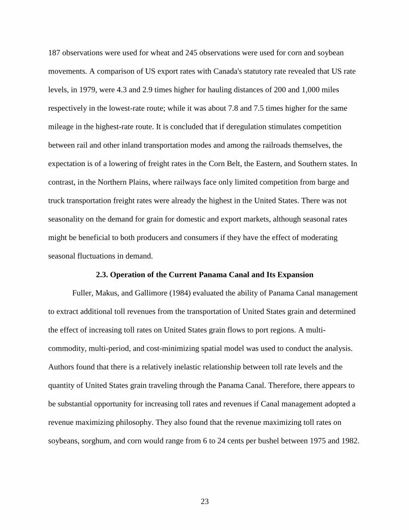
Figure 3.1 represents effects of transportation costs from an exporting country to an
importing country. Figure 3.1 (a) shows domestic demand and supply in an importing country
and Figure 3.1 (c) represents domestic demand and supply in an exporting country. Figure 3.1 (b)
shows export supply and import demand in international market. In Figure 3.1 (b), an
international equilibrium price of goods without transportation costs is P and the quantity traded
is OQ. Transportation costs are represented by distance ab, which is equal to (P1 - P2). Given this
transportation cost, the price in the importing country increases from P to P1, and the price in the
exporting country decreases from P to P2. The price difference between the two countries, (P1 -
P2), is transportation costs in a free market system. Since the price of goods in the importing
country increases and the price of goods in exporting country decreases, the trade volume
decreases from Q to QI. This trade volume is equal to country’s imports and country’s exports.
The decrease in the price of goods in the exporting country is the portion of transportation costs
29
that producers pay in the exporting country. The increase in price of goods in the importing
country is the portion of transportation costs that consumers pay in the importing country. This
implies that transportation costs are shared between the two countries, depending upon the price
elasticity of export supply and import demand. However, transportation costs are measured by
TEU, rather than the actual price of goods because it is not possible to evaluate the value of
goods in containers for every containerized shipment. Therefore, the value of goods in containers
is ignored for this study since various types of cargo are containerized.
Figure 3.1. Effects of Transportation Cost (Koo, 1984).
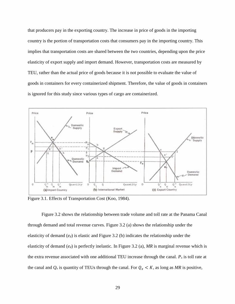
Figure 3.2 shows the relationship between trade volume and toll rate at the Panama Canal
through demand and total revenue curves. Figure 3.2 (a) shows the relationship under the
elasticity of demand (ed) is elastic and Figure 3.2 (b) indicates the relationship under the
elasticity of demand (ed) is perfectly inelastic. In Figure 3.2 (a), MR is marginal revenue which is
the extra revenue associated with one additional TEU increase through the canal. Px is toll rate at
the canal and Qx is quantity of TEUs through the canal. For 𝑄𝑥 < 𝐾, as long as MR is positive,
30
meaning every additional TEU will increase the total revenue. However, MR gets smaller as
output increases. Thus, the total revenue increases at a decreasing rate. Eventually, at the
midpoint (C) of the linear demand curve, 𝑀𝑅 = 0. This implies that the total revenue neither
increases nor decreases. For 𝑄𝑥 > 𝐾, 𝑀𝑅 < 0, indicating that every additional TEU will
decrease the total revenue. In Figure 3.2 (b), since changes in quantity are not sensitive to
changes in price, the total revenue increases as the price increases. Marginal revenue (MR) is
equal to demand. As a result, an optimal price to maximize the total revenue is inconclusive
when the elasticity of demand is perfectly inelastic.
Figure 3.2. Relationship between trade volume and toll rate at the Panama Canal.

31
Throughput demand through the PNC (Figure 3.2 (a)) can be expressed as follows:
𝑄𝑥 = 𝛼 − 𝛽𝑃𝑥 (3.1)
where 𝑄𝑥 is the quantity shipped through the PNC and 𝑃𝑥 is toll rate at the canal.
𝑇𝑅 = 𝑃𝑥 ∗ 𝑄𝑥 = (𝛼 − 𝛽𝑃𝑥) ∗ 𝑃𝑥 = 𝛼𝑃𝑥 − 𝛽𝑃𝑥2 (3.2)
MR is obtained by taking partial derivative of TR with respect to 𝑃𝑥 as follows:
𝜕𝑇𝑅
𝜕(𝑃𝑥)= 𝛼 − 2𝛽(𝑃𝑥)
(3.3)
To find the toll rate to maximize TR, set 𝑀𝑅 = 0 as follows:
𝛼 − 2𝛽(𝑃𝑥) = 0 (3.4)
𝑃𝑥 =𝛼
2𝛽
(3.5)
3.2. Basic Structure of Container Shipment Model
The model used for this study is developed on the basis of a mathematical programming
model based on a linear programming algorithm. The objective of the model is to minimize
transportation and handling costs of containers from shipping origin to destination. The objective
function is optimized subject to a set of linear equations, representing the supply of containerized
cargo at shipping origins in exporting countries and demand for the cargo in importing countries.
Inland transportation modes used in this study are rail, truck, and barge. In general, trucks are the
cheapest transportation mode for shipping containers short distances, followed by rail (Figure
3.3). For this reason, trucks and rails will be used to ship domestic containers from shipping
origins/destinations to/from container ports in the United States. Since barges are the cheapest
mode of transportation for long distances, rail and barges will be used for long-distance hauling.

32
Figure 3.3. Hypothetical trip cost curves for rail (RR’), truck (TT’), and barge (WW’) modes of
transportation for a given origin/destination (Koo, Tolliver, and Bitzan, 1993).
In Figure 3.3, the industry has a comparative advantage in section OC, railways in
section CD, and barges in distances greater than OD. Container vessels are the primary ocean
transportation mode for shipping containers from ports in exporting countries to ports in
importing countries. Figure 3.4 shows the classification of container ship by its capacity. As
shown in Figure 3.4, the maximum container vessel size through the Panama Canal will increase
from 4,500 TEUs to 12,500 TEUs, three times larger than the current Panamax allowance.

33
Figure 3.4. Classification of container vessel by its capacity (in meters) (Ashar and Rodrigue,
2012).
3.3. Model Description
Set:
SO = set of shipping origins for US exports in the United States
EPe = set of export ports for US exports in the United States
RPe = set of river ports for US exports in the United States
IPe = set of import ports for US exports in importing countries
EPi = set of export ports for US imports in exporting countries
IPi = set of import ports for US imports in the United States
RPi = set of river ports for US imports in the United States
SD = set of shipping destinations for US imports in the United States
Parameters:
Dq = demand of TEUs for US exports in importing countries, 𝑞 ∈ 𝐼𝑃𝑒

34
Qi = supply of TEUs for US exports in shipping origins, 𝑖 ∈ 𝑆𝑂
Dd = demand of TEUs for US imports in shipping destinations, 𝑑 ∈ 𝑆𝐷
Qf = supply of TEUs for US imports in exporting countries, 𝑓 ∈ 𝐸𝑃𝑖
PCp = cargo handling capacity (TEUs) at export ports in the United States, 𝑝 ∈ 𝐸𝑃𝑒
PCu = cargo handling capacity (TEUs) at import ports in the United States, 𝑢 ∈ 𝐼𝑃𝑖
PC = aggregated cargo handling capacity (TEUs) at ports in the United States
PCC = cargo handling capacity (TEUs) at the Panama Canal
𝑇𝑡 = truck freight rate per TEU in the United States
𝑇𝑟 = rail freight rate per TEU in the United States
𝑇𝑏 = barge freight rate per TEU in the United States
𝑇𝑜 = ocean freight rate per TEU without the Panama Canal
𝑇𝑜𝑐 = ocean freight rate per TEU through the Panama Canal
h = cargo handling charge per TEU at ports in exporting and importing countries
𝜌 = toll rate per TEU at the Panama Canal
𝜎 = delay cost per TEU at the Panama Canal
Decision variables:
𝑄𝑡 = the quantity of TEUs shipped by truck
𝑄𝑟 = the quantity of TEUs shipped by rail
𝑄𝑏 = the quantity of TEUs shipped by barge
𝑄𝑜 = the quantity of TEUs shipped by container vessel without the Panama Canal
𝑄𝑜𝑐 = the quantity of TEUs shipped by container vessel through the Panama Canal

35
3.4. Spatial Optimization Model for US Exports
The model developed for US exports includes shipping origins and export ports in the
United States and major container ports in importing countries, especially Northeast Asia and
Europe. Shipping origin of each is identified based on workforce. Major container importing
countries are chosen on the basis of their import volume from the United States. The model
includes several inland transportation modes in the United States to evaluate the effects of
intermodal competition on optimal container shipments for export in the United States. The
model also includes major container ports in the United States for international trade. These ports
will be used in the transit of containers from shipping origins in the United States to ports in
importing countries.
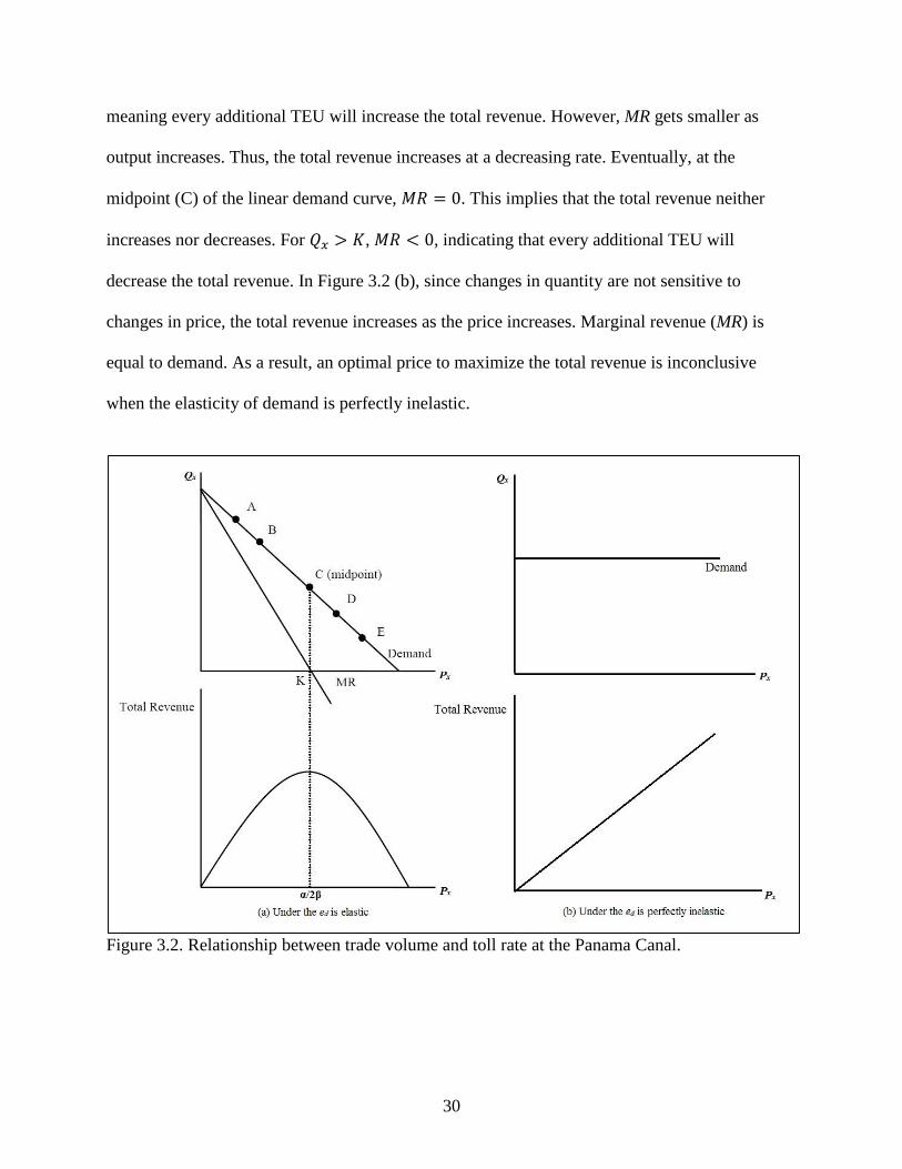
Figure 3.5 represents the supply chain of container shipments from shipping origins to
export ports and from export ports to ports in importing countries either with or without the
Panama Canal. Rails and trucks are considered as transportation for shipping containers from
shipping origins to export ports and a truck-barge combination is also considered as an inland
transportation mode in the United States. The truck-barge combination consists of transiting
containers from shipping origins to the river ports by truck and from the river ports to the US
Gulf ports by barge. Container vessels are available for the ocean transportation mode and it
navigates on a route either with or without the Panama Canal. Different sizes of container vessels
are used for this study because the Panama Canal and container ports of exporting and importing
countries have a size limitation of vessel that can be handled at their facilities.
36
Figure 3.5. Regions associated with container trade and transportation modes for US exports.
The domestic transportation system in the United States is optimized by using a linear
programing model. The objective function of the spatial optimization model is to minimize
transportation and handling costs in shipping containers from shipping origins to export ports in
the United States. The objective function is specified as follows:
𝑊𝑒𝑙 = ∑ ∑ 𝑄𝑖𝑝𝑡 𝑇𝑖𝑝
𝑡
𝑃
𝑝=1
𝐼
𝑖=1
+ ∑ ∑ 𝑄𝑖𝑝𝑟 𝑇𝑖𝑝
𝑟
𝑃
𝑝=1
𝐼
𝑖=1
+ ∑ ∑ 𝑄𝑖𝑎𝑡 𝑇𝑖𝑎
𝑡
𝐴
𝑎=1
𝐼
𝑖=1
+ ∑ ∑ 𝑄𝑎𝑝𝑏 𝑇𝑎𝑝
𝑏
𝑃
𝑝=1
𝐴
𝑎=1
(3.6)
where i is an index for shipping origins in the United States, p is an index for export ports in the
United States, t is an index for truck transportation mode, r is an index for rail transportation
mode, b is an index for barge transportation mode, a is an index for barge access points, and T
represents transportation costs. 𝑄𝑖𝑝𝑡 is containers (TEUs) shipped from shipping origin i to export
port p by trucks, 𝑄𝑖𝑝𝑟 is containers (TEUs) shipped from shipping origin i to export port p by rails,
Ocean TransitInland Transit
Shipping Origin i
Export Port p
Panama Canal
Import Port q
𝑚𝑖𝑎𝑝- truck-barge combination
𝑚𝑖𝑝 – Rail/Truck
𝑣𝑝𝑞 – Container Ship
𝑣𝑝𝑐𝑞 – Container Ship

37
𝑄𝑖𝑎𝑡 is containers (TEUs) shipped from shipping origin i to barge access point a by trucks, 𝑄𝑎𝑝
𝑏 is
containers (TEUs) shipped from barge point a to export port p by barges, 𝑇𝑖𝑝𝑡 is transportation
costs from shipping origin i to export port p by trucks, 𝑇𝑖𝑝𝑟 is transportation costs from shipping
origin i to export port p by rails, 𝑇𝑖𝑎𝑡 is transportation costs from shipping origin i to barge access
point a by trucks, and 𝑇𝑎𝑝𝑏 is transportation costs from barge access point a to export port p by
barges.
Inland transportation costs in the United States consist of costs from shipping origins to
export ports. When several transportation modes are available, the least expensive mode is
chosen for container shipments. The first and second terms of Equation 3.6 represent the sum of
transportation costs in shipping containers from shipping origins to export ports by trucks and
rails, respectively; the third term represents shipment of containers from shipping origins to
barge access points by truck; and the last term represents shipment of containers from barge
access points to export ports by barge.
The international transportation system from the United States to importing countries is
optimized by using a linear programing model. The objective function of the spatial optimization
model is to minimize transportation and handling costs in shipping containers from US origins to
import ports. The objective function is specified as follows:
𝑊𝑒𝑜 = ∑ ∑ 𝑄𝑝𝑞𝑜 (𝑇𝑝𝑞
𝑜
𝑄
𝑞=1
𝑃
𝑝=1
+ ℎ𝑝𝑞) + ∑ ∑ 𝑄𝑝𝑞𝑜𝑐
𝑄
𝑞=1
𝑃
𝑝=1
(𝑇𝑝𝑞𝑜𝑐 + 𝜌 + 𝜎) (3.7)
where p is index for major container ports in the United States, q is an index for major container
ports in importing countries, 𝑄𝑝𝑞𝑜 is containers (TEUs) shipped from US port p to import port q
without the Panama Canal, 𝑄𝑝𝑞𝑜𝑐 is containers (TEUs) shipped from US port p to import port q
through the Panama Canal, 𝑇𝑝𝑞𝑜 is ocean transportation costs by ship size from US port p to

38
import port q without using the canal, 𝑇𝑝𝑞𝑜𝑐 is ocean transportation costs by ship size from US port
p to import port q through the canal, ℎ𝑝𝑞 is the handling charge at ports p and q, 𝜌 is the toll rate
per TEU at the Panama Canal, and 𝜎 is the delay cost per TEU at the Panama Canal.
Ocean transportation costs between the United States and importing countries consist of
costs from US ports to import ports. Since two ocean routes for container shipments are available,
the least expensive route is chosen for container shipments. The first term of Equation 3.7
represents the sum of transportation costs from US ports to import ports without using the
Panama Canal and handling costs at ports in US and it trade partners. The next term indicates the
sum of transportation costs from US ports to import ports through the Panama Canal, handling
costs at the ports in the US and its importing countries, the PNC toll rate, and the delay cost at
the Panama Canal.
Since the objective of this study is to optimize container flows from shipping origins in
the United States to import ports in importing countries, under the spatial optimization and the
objective function of the spatial optimization model for US export the sum of equations 3.7 and
3.8 is as follows:
𝑊𝑒 = ∑ ∑ 𝑄𝑖𝑝𝑡 𝑇𝑖𝑝
𝑡
𝑃
𝑝=1
𝐼
𝑖=1
+ ∑ ∑ 𝑄𝑖𝑝𝑟 𝑇𝑖𝑝
𝑟
𝑃
𝑝=1
𝐼
𝑖=1
+ ∑ ∑ 𝑄𝑖𝑎𝑡 𝑇𝑖𝑎
𝑡
𝐴
𝑎=1
𝐼
𝑖=1
+ ∑ ∑ 𝑄𝑎𝑝𝑏 𝑇𝑎𝑝
𝑏
𝑃
𝑝=1
𝐴
𝑎=1
+ ∑ ∑ 𝑄𝑝𝑞𝑜 (𝑇𝑝𝑞
𝑜
𝑄
𝑞=1
𝑃
𝑝=1
+ ℎ𝑝𝑞) + ∑ ∑ 𝑄𝑝𝑞𝑜𝑐
𝑄
𝑞=1
𝑃
𝑝=1
(𝑇𝑝𝑞𝑜𝑐 + 𝜌 + 𝜎)
(3.8)
Transportation costs are divided into domestic transportation and ocean transportation costs.
Ocean shipments are divided into shipments from the United States to importing countries
whether the shipments pass through the Panama Canal. Handling charges such as loading and

39
unloading, at the ports in exporting and importing countries, the PNC toll, and the delay cost at
the canal are included in the objective function.
Major constraints of the model are domestic supply in the United States, import demand
in importing countries, cargo handling capacities of U.S ports and the Panama Canal and the
inventory-clearing condition at export and import ports. The constraints are presented as follows:
∑ 𝑄𝑝𝑞𝑜
𝑃
𝑝=1
+ ∑ 𝑄𝑝𝑞𝑜𝑐
𝑃
𝑝=1
≥ 𝐷𝑞 (3.9)
∑ 𝑄𝑖𝑝𝑡
𝑃
𝑝=1
+ ∑ 𝑄𝑖𝑝𝑟
𝑃
𝑝=1
+ ∑ 𝑄𝑖𝑎𝑡
𝐴
𝑎=1
≤ 𝑄𝑖 (3.10)
∑ 𝑄𝑖𝑝
𝐼
𝑖=1
≤ 𝑃𝐶𝑝 (3.11)
∑ ∑ 𝑄𝑝𝑞𝑜𝑐
𝑄
𝑞=1
𝑃
𝑝=1
≤ 𝑃𝐶𝐶 (3.12)
𝑄𝑞 = ∑ 𝑄𝑝𝑞𝑜
𝑄
𝑞=1
+ ∑ 𝑄𝑝𝑞𝑜𝑐
𝑄
𝑞=1
, 𝑞 = 1,2, … , 𝑄 (3.13)
𝑄𝑝 = ∑ 𝑄𝑖𝑝𝑡
𝐼
𝑖=1
+ ∑ 𝑄𝑖𝑝𝑟
𝐼
𝑖=1
+ ∑ 𝑄𝑎𝑝𝑏
𝐼
𝑖=1
, 𝑝 = 1,2, … , 𝑃 (3.14)
𝑄𝑎𝐺𝑢𝑙𝑓𝑏 = ∑ 𝑄𝑖𝑎
𝑡
𝐼
𝑖=1
, 𝑎 = 1,2, … , 𝐴 𝑎𝑛𝑑 𝑎 ∈ 𝑅𝑃𝑒 (3.15)
𝑄𝑝 = ∑ 𝑄𝑝𝑞𝑜
𝑃
𝑝=1
+ ∑ 𝑄𝑝𝑞𝑜𝑐
𝑃
𝑝=1
, 𝑝 = 1,2, … , 𝑃
(3.16)
where 𝑄𝑞 is the number of containers (TEUs) at import port q, 𝑄𝑝 is the number of containers
(TEUs) at export port p, and 𝑄𝑎𝐺𝑢𝑙𝑓𝑏 is the number of containers for the Gulf ports at barge access

40
points a. Other variables are defined previously. Equations 3.9 and 3.10 represent import demand
and export supply constraints respectively. Equation 3.9 represents the import demand
constraints in importing countries. Equation 3.10 indicates that the total containers shipped from
each shipping origins in the United States should be equal to or smaller than the quantities of
containers shipped to the export ports. Equations 3.11 and 3.12 represent container handling
capacities at ports in the United States and the Panama Canal, respectively. The total quantities
of containers handled by each port and the Panama Canal should be equal to or smaller than
handling capacities at their facilities. Equation 3.13 indicates that the quantity of containers
imported in import port q is equal to the sum of containers shipped from export ports. Equation
3.14 describes that the quantity of container exported in port p is equal to quantity of containers
received from either shipping origins by truck and rail or barge access points by barge. Equation
3.15 is an inventory clearing condition at barge access points indicating that the quantity of
containers received in each barge access points by truck should be equal to the quantity shipped
out by barge to the Gulf ports. Equation 3.16 also describes an inventory-clearing condition at
ports, indicating that the container quantities received by each export port from shipping origins
must equal to the container quantities shipped to each import port.
3.5. Spatial Optimization Model for US Imports
The model developed for US imports includes major shipping destinations and container
ports in the United States and ports in exporting countries. Major container shipping destinations
will be identified as one of each states of the US mainland, based on population. Major container
exporting countries are identified on the basis of US import volume. The model includes several
inland transportation modes in the United States to evaluate the effects of intermodal competition
on optimal container shipments in the United States. Ports in the United States will be used in the

41
transit of containers from ports in exporting countries to shipping destinations in the United
States.
Figure 3.6. Regions associated with container trade and transportation modes for US imports.
Figure 3.6 represents the supply chain of container shipments from export ports in other
countries to shipping destinations at US imports. Ocean vessels are the transportation mode used
for shipping containers from ports in exporting countries to ports in the United States. The model
for import includes barges, as one of the inland transportation modes, which are available to ship
containers from the US Gulf ports to water access points along major US river systems. Since
barges are the cheapest mode of inland transportation for long distances, barges are used for
long-distance hauling. Containers imported in the Gulf ports in the United States can be moved
to water access points by barge and then moved to shipping destinations by truck, called a truck-
barge combination. For shipment from other US import ports, either rails or trucks are used to
Inland TransitOcean Transit
Export Port f
Panama Canal
Import Port uShipping
Destination
d
𝑚𝑢𝑑 – Rail/Truck/Truck-Barge Combination 𝑣𝑓𝑢 – Container Ship

42
ship containers since trucks are the cheapest transportation mode for shipping containers short
distances, followed by rail in general.
The international transportation system from exporting countries to the United States is
optimized by using a linear programing model. The objective function of the spatial optimization
model is to minimize transportation and handling costs in shipping containers from export ports
to US ports. The objective function is specified as follows:
𝑊𝑖𝑜 = ∑ ∑ 𝑄𝑓𝑢𝑜 (𝑇𝑓𝑢
𝑜
𝑈
𝑢=1
𝐹
𝑓=1
+ ℎ𝑓𝑢) + ∑ ∑ 𝑄𝑓𝑢𝑜𝑐
𝑈
𝑢=1
𝐹
𝑓=1
(𝑇𝑓𝑢𝑜𝑐 + 𝜌 + 𝜎) (3.17)
where f is the index for ports in exporting countries, u is an index for container ports in the
United States, 𝑄𝑓𝑢𝑜 is containers (TEUs) shipped from export port f to US port u without the
Panama Canal, 𝑄𝑓𝑢𝑜𝑐 is containers (TEUs) shipped from export f to US port u through the Panama
Canal, 𝑇𝑓𝑢𝑜 is ocean transportation costs by ship size from export port f to US port u without
using the canal, 𝑇𝑓𝑢𝑜𝑐 is ocean transportation costs by ship size from export port f to US port u
through the canal, ℎ𝑓𝑢 is handling charges at ports f and u , 𝜌 is the toll rate per TEU at the
Panama Canal, and 𝜎 is the delay cost per TEU at the Panama Canal.
Ocean transportation costs between exporting countries and the United States consist of
costs from export ports to US ports. Since two ocean routes for container shipments are available,
the least expensive route is chosen for container shipments. The first term of equation 3.17
represents the sum of ocean transportation costs from export ports to US ports without the
Panama Canal and handling costs at the ports in exporting and importing countries. The next
term indicates the sum of transportation costs from export ports to US ports through the Panama
Canal, handling costs at ports, the PNC toll, and delay costs at the Panama Canal.
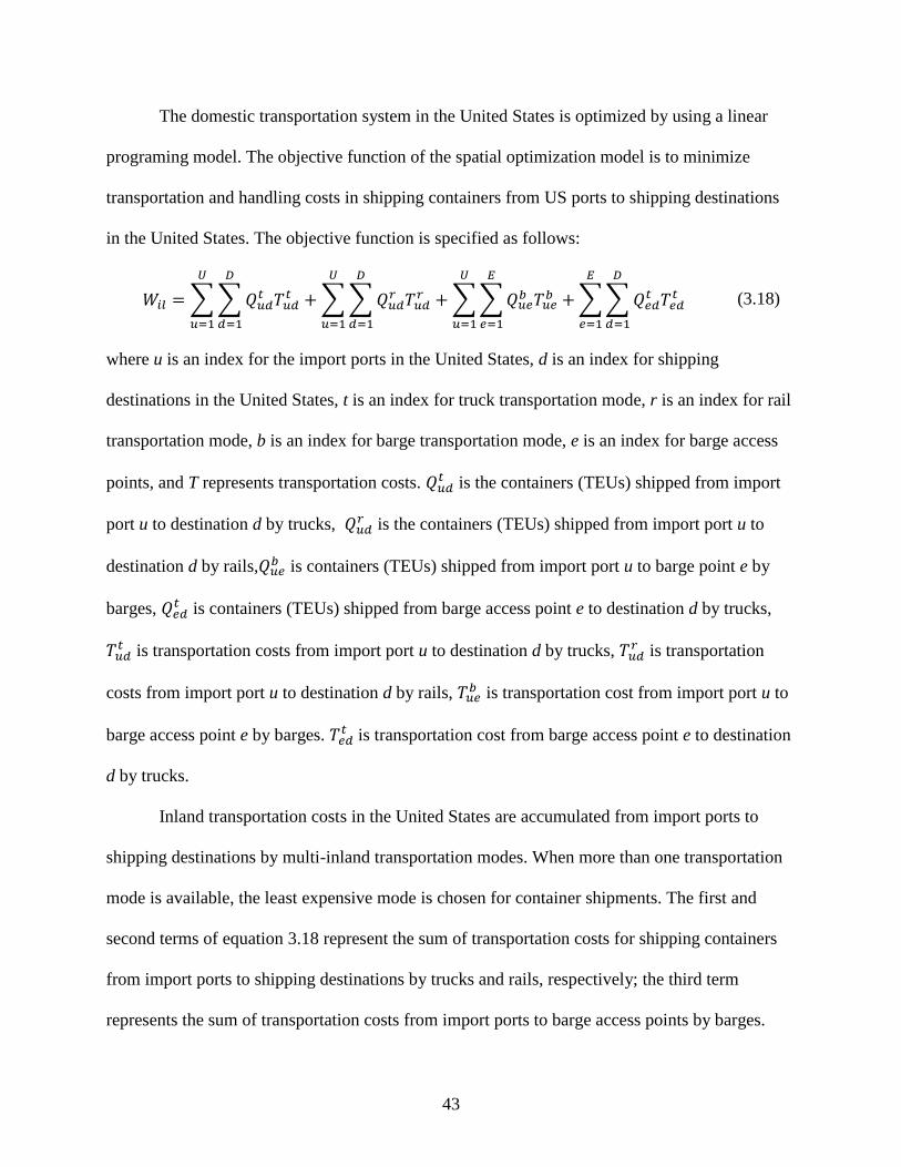
43
The domestic transportation system in the United States is optimized by using a linear
programing model. The objective function of the spatial optimization model is to minimize
transportation and handling costs in shipping containers from US ports to shipping destinations
in the United States. The objective function is specified as follows:
𝑊𝑖𝑙 = ∑ ∑ 𝑄𝑢𝑑𝑡 𝑇𝑢𝑑
𝑡
𝐷
𝑑=1
𝑈
𝑢=1
+ ∑ ∑ 𝑄𝑢𝑑𝑟 𝑇𝑢𝑑
𝑟
𝐷
𝑑=1
𝑈
𝑢=1
+ ∑ ∑ 𝑄𝑢𝑒𝑏 𝑇𝑢𝑒
𝑏
𝐸
𝑒=1
𝑈
𝑢=1
+ ∑ ∑ 𝑄𝑒𝑑𝑡 𝑇𝑒𝑑
𝑡
𝐷
𝑑=1
𝐸
𝑒=1
(3.18)
where u is an index for the import ports in the United States, d is an index for shipping
destinations in the United States, t is an index for truck transportation mode, r is an index for rail
transportation mode, b is an index for barge transportation mode, e is an index for barge access
points, and T represents transportation costs. 𝑄𝑢𝑑𝑡 is the containers (TEUs) shipped from import
port u to destination d by trucks, 𝑄𝑢𝑑𝑟 is the containers (TEUs) shipped from import port u to
destination d by rails,𝑄𝑢𝑒𝑏 is containers (TEUs) shipped from import port u to barge point e by
barges, 𝑄𝑒𝑑𝑡 is containers (TEUs) shipped from barge access point e to destination d by trucks,
𝑇𝑢𝑑𝑡 is transportation costs from import port u to destination d by trucks, 𝑇𝑢𝑑
𝑟 is transportation
costs from import port u to destination d by rails, 𝑇𝑢𝑒𝑏 is transportation cost from import port u to
barge access point e by barges. 𝑇𝑒𝑑𝑡 is transportation cost from barge access point e to destination
d by trucks.
Inland transportation costs in the United States are accumulated from import ports to
shipping destinations by multi-inland transportation modes. When more than one transportation
mode is available, the least expensive mode is chosen for container shipments. The first and
second terms of equation 3.18 represent the sum of transportation costs for shipping containers
from import ports to shipping destinations by trucks and rails, respectively; the third term
represents the sum of transportation costs from import ports to barge access points by barges.
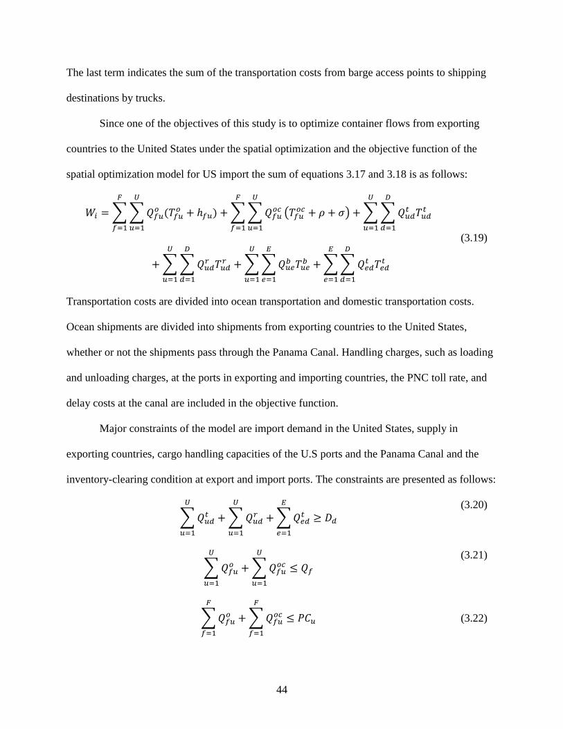
44
The last term indicates the sum of the transportation costs from barge access points to shipping
destinations by trucks.
Since one of the objectives of this study is to optimize container flows from exporting
countries to the United States under the spatial optimization and the objective function of the
spatial optimization model for US import the sum of equations 3.17 and 3.18 is as follows:
𝑊𝑖 = ∑ ∑ 𝑄𝑓𝑢𝑜 (𝑇𝑓𝑢
𝑜
𝑈
𝑢=1
𝐹
𝑓=1
+ ℎ𝑓𝑢) + ∑ ∑ 𝑄𝑓𝑢𝑜𝑐
𝑈
𝑢=1
𝐹
𝑓=1
(𝑇𝑓𝑢𝑜𝑐 + 𝜌 + 𝜎) + ∑ ∑ 𝑄𝑢𝑑
𝑡 𝑇𝑢𝑑𝑡
𝐷
𝑑=1
𝑈
𝑢=1
+ ∑ ∑ 𝑄𝑢𝑑𝑟 𝑇𝑢𝑑
𝑟
𝐷
𝑑=1
𝑈
𝑢=1
+ ∑ ∑ 𝑄𝑢𝑒𝑏 𝑇𝑢𝑒
𝑏
𝐸
𝑒=1
𝑈
𝑢=1
+ ∑ ∑ 𝑄𝑒𝑑𝑡 𝑇𝑒𝑑
𝑡
𝐷
𝑑=1
𝐸
𝑒=1
(3.19)
Transportation costs are divided into ocean transportation and domestic transportation costs.
Ocean shipments are divided into shipments from exporting countries to the United States,
whether or not the shipments pass through the Panama Canal. Handling charges, such as loading
and unloading charges, at the ports in exporting and importing countries, the PNC toll rate, and
delay costs at the canal are included in the objective function.
Major constraints of the model are import demand in the United States, supply in
exporting countries, cargo handling capacities of the U.S ports and the Panama Canal and the
inventory-clearing condition at export and import ports. The constraints are presented as follows:
∑ 𝑄𝑢𝑑𝑡
𝑈
𝑢=1
+ ∑ 𝑄𝑢𝑑𝑟
𝑈
𝑢=1
+ ∑ 𝑄𝑒𝑑𝑡
𝐸
𝑒=1
≥ 𝐷𝑑
(3.20)
∑ 𝑄𝑓𝑢𝑜
𝑈
𝑢=1
+ ∑ 𝑄𝑓𝑢𝑜𝑐
𝑈
𝑢=1
≤ 𝑄𝑓
(3.21)
∑ 𝑄𝑓𝑢𝑜
𝐹
𝑓=1
+ ∑ 𝑄𝑓𝑢𝑜𝑐
𝐹
𝑓=1
≤ 𝑃𝐶𝑢 (3.22)

45
∑ ∑ 𝑄𝑓𝑢𝑜𝑐
𝑈
𝑢=1
𝐹
𝑓=1
≤ 𝑃𝐶𝐶
(3.23)
𝑄𝑢 = ∑ 𝑄𝑓𝑢𝑜
𝑈
𝑢=1
+ ∑ 𝑄𝑓𝑢𝑜𝑐
𝑈
𝑢=1
, 𝑢 = 1,2, … , 𝑈
(3.24)
𝑄𝑑 = ∑ 𝑄𝑢𝑑𝑡
𝐷
𝑑=1
+ ∑ 𝑄𝑢𝑑𝑟
𝐷
𝑑=1
+ ∑ 𝑄𝑒𝑑𝑡
𝐷
𝑑=1
, 𝑑 = 1,2, … , 𝐷 (3.25)
𝑄𝑢 = ∑ 𝑄𝑢𝑑𝑡
𝐷
𝑑=1
+ ∑ 𝑄𝑢𝑑𝑟
𝐷
𝑑=1
+ ∑ 𝑄𝑢𝑒𝑏
𝐷
𝑑=1
, 𝑢 = 1,2, … , 𝑈 (3.26)
𝑄𝐺𝑢𝑙𝑓,𝑒𝑏 = ∑ 𝑄𝑒𝑑
𝑡
𝐷
𝑑=1
, 𝑒 = 1,2, … , 𝐸 𝑎𝑛𝑑 𝑒 ∈ 𝑅𝑃𝑖 (3.27)
where 𝑄𝑢 is the number of containers (TEUs) at import port u, 𝑄𝑑 is the number of containers
(TEUs) at destination d, 𝑄𝐺𝑢𝑙𝑓,𝑒𝑏 is the number of containers from the Gulf ports to barge access
points e. Other variables are defined previously.
Equations 3.20 and 3.21 represent import demand and export supply constraints
respectively. Equation 3.20 represents the import demand constraints in the United States.
Equation 3.21 indicates that the total containers shipped from ports in exporting countries should
be equal to or smaller than the quantities of containers shipped to the United States. Equations
3.22 and 3.23 represent container handling capacities at ports in the United States and the
Panama Canal, respectively. The total quantities of containers handled by each port and the
Panama Canal should be equal to or smaller than their annual handling capacities. Equation 3.24
indicates that the quantity of containers received at import port u is equal to the sum of
containers shipped from export ports. Equation 3.25 describes that the quantity of containers
received at destination d is equal to sum of the containers from import ports and barge access

46
points. Equation 3.26 describes an inventory-clearing condition at ports, indicating that the
container quantities received by each import port from exporting countries must equal to sum of
containers shipped to destinations and barge access points. Equation 3.27 is an inventory clearing
condition at barge access points indicating that the quantity of containers received in each barge
access point by barge from the Gulf ports should be equal to the quantity shipped out through
trucks to destinations.
3.6. Spatial Optimization Model for US Container Trade
Since a primary objective of this study is to optimize overall flows of containerized
shipment in the United States, export and import were considered at the same time. Therefore,
the objective function of the spatial optimization model for this study is developed by combining
equations 3.8 and 3.19 as follows:
𝑊𝑐 = ∑ ∑ 𝑄𝑖𝑝𝑡 𝑇𝑖𝑝
𝑡
𝑃
𝑝=1
𝐼
𝑖=1
+ ∑ ∑ 𝑄𝑖𝑝𝑟 𝑇𝑖𝑝
𝑟
𝑃
𝑝=1
𝐼
𝑖=1
+ ∑ ∑ 𝑄𝑖𝑎𝑡 𝑇𝑖𝑎
𝑡
𝐴
𝑎=1
𝐼
𝑖=1
+ ∑ ∑ 𝑄𝑎𝑝𝑏 𝑇𝑎𝑝
𝑏
𝑃
𝑝=1
𝐴
𝑎=1
+ ∑ ∑ 𝑄𝑢𝑑𝑡 𝑇𝑢𝑑
𝑡
𝐷
𝑑=1
𝑈
𝑢=1
+ ∑ ∑ 𝑄𝑢𝑑𝑟 𝑇𝑢𝑑
𝑟
𝐷
𝑑=1
𝑈
𝑢=1
+ ∑ ∑ 𝑄𝑢𝑒𝑏 𝑇𝑢𝑒
𝑏
𝐸
𝑒=1
𝑈
𝑢=1
+ ∑ ∑ 𝑄𝑒𝑑𝑡 𝑇𝑒𝑑
𝑡
𝐷
𝑑=1
𝐸
𝑒=1
+ ∑ ∑ 𝑄𝑝𝑞𝑜 (𝑇𝑝𝑞
𝑜
𝑄
𝑞=1
𝑃
𝑝=1
+ ℎ𝑝𝑞)
+ ∑ ∑ 𝑄𝑝𝑞𝑜𝑐
𝑄
𝑞=1
𝑃
𝑝=1
(𝑇𝑝𝑞𝑜𝑐 + 𝜌 + 𝜎) + ∑ ∑ 𝑄𝑓𝑢
𝑜𝑐
𝑈
𝑢=1
𝐹
𝑓=1
(𝑇𝑓𝑢𝑜𝑐 + 𝜌 + 𝜎)
+ ∑ ∑ 𝑄𝑝𝑞𝑜 (𝑇𝑓𝑢
𝑜
𝑈
𝑢=1
𝐹
𝑓=1
+ ℎ𝑓𝑢)
(3.28)
The first through fourth terms represent inland transportation costs for US exports and the fifth
through eighth terms are inland transportation costs for US imports. The last four terms represent

47
ocean transportation costs of containerized shipments for US exports and imports and those
include cargo handling charges at ports in exporting and importing countries, the PNC toll rate,
and the delay cost at the Panama Canal.
Major constraints of the model are import demand in importing countries, supply in
exporting countries, cargo handling capacity at US ports and the Panama Canal, and the
inventory-clearing condition at US ports. The constraints are presented as follows:
∑ 𝑄𝑝𝑞𝑜
𝑃
𝑝=1
+ ∑ 𝑄𝑝𝑞𝑜𝑐
𝑃
𝑝=1
≥ 𝐷𝑞 (3.29)
∑ 𝑄𝑢𝑑𝑡
𝑈
𝑢=1
+ ∑ 𝑄𝑢𝑑𝑟
𝑈
𝑢=1
+ ∑ 𝑄𝑒𝑑𝑡
𝐸
𝑒=1
≥ 𝐷𝑑 (3.30)
∑ 𝑄𝑖𝑝𝑡
𝑃
𝑝=1
+ ∑ 𝑄𝑖𝑝𝑟
𝑃
𝑝=1
+ ∑ 𝑄𝑖𝑎𝑡
𝐴
𝑎=1
≤ 𝑄𝑖 (3.31)
∑ 𝑄𝑓𝑢𝑜
𝑈
𝑢=1
+ ∑ 𝑄𝑓𝑢𝑜𝑐
𝑈
𝑢=1
≤ 𝑄𝑓 (3.32)
∑ 𝑄𝑖𝑝
𝐼
𝑖=1
+ ∑ 𝑄𝑎𝑝
𝐴
𝑎=1
+ ∑ 𝑄𝑓𝑢𝑜
𝐹
𝑓=1
+ ∑ 𝑄𝑓𝑢𝑜𝑐
𝐹
𝑓=1
≤ 𝑃𝐶 , 𝑝 = 𝑢 (3.33)
∑ ∑ 𝑄𝑝𝑞𝑜𝑐
𝑄
𝑞=1
𝑃
𝑝=1
+ ∑ ∑ 𝑄𝑓𝑢𝑜𝑐
𝑈
𝑢=1
𝐹
𝑓=1
≤ 𝑃𝐶𝐶 (3.34)
𝑄𝑞 = ∑ 𝑄𝑝𝑞
𝑃
𝑝=1
, 𝑞 = 1,2, … , 𝑄 (3.35)
𝑄𝑝 = ∑ 𝑄𝑖𝑝𝑡
𝐼
𝑖=1
+ ∑ 𝑄𝑖𝑝𝑟
𝐼
𝑖=1
+ ∑ 𝑄𝑎𝑝𝑏
𝐼
𝑖=1
, 𝑝 = 1,2, … , 𝑃 (3.36)

48
𝑄𝑎𝐺𝑢𝑙𝑓𝑏 = ∑ 𝑄𝑖𝑎
𝑡
𝐼
𝑖=1
, 𝑎 = 1,2, … , 𝐴 𝑎𝑛𝑑 𝑎 ∈ 𝑅𝑃𝑒 (3.37)
𝑄𝑝 = ∑ 𝑄𝑝𝑞
𝑄
𝑞=1
, 𝑝 = 1,2, … , 𝑃 (3.38)
𝑄𝑢 = ∑ 𝑄𝑓𝑢
𝐹
𝑓=1
, 𝑢 = 1,2, … , 𝑈 (3.39)
𝑄𝑑 = ∑ 𝑄𝑢𝑑𝑡
𝐷
𝑑=1
+ ∑ 𝑄𝑢𝑑𝑟
𝐷
𝑑=1
+ ∑ 𝑄𝑒𝑑𝑡
𝐷
𝑑=1
, 𝑑 = 1,2, … , 𝐷 (3.40)
𝑄𝑢 = ∑ 𝑄𝑢𝑑𝑡
𝐷
𝑑=1
+ ∑ 𝑄𝑢𝑑𝑟
𝐷
𝑑=1
+ ∑ 𝑄𝑢𝑒𝑏
𝐷
𝑑=1
, 𝑢 = 1,2, … , 𝑈
(3.41)
𝑄𝐺𝑢𝑙𝑓,𝑒𝑏 = ∑ 𝑄𝑒𝑑
𝑡
𝐷
𝑑=1
, 𝑒 = 1,2, … , 𝐸 𝑎𝑛𝑑 𝑒 ∈ 𝑅𝑃𝑖 (3.42)
where 𝑃𝐶 is annual handling capacity of container ports in the United States. Other variables are
defined previously.
Equations 3.29 and 3.30 represent import demands in importing countries for US exports
and the United States for US imports, respectively. Equations 3.31 and 3.32 represent export
supply constraints in the United States for US exports and exporting countries for US imports,
respectively. Equations 3.33 and 3.34 represent containers handling capacities at US ports and
the Panama Canal, respectively. The total quantities of containers handled by each port and the
Panama Canal should be equal to or smaller than their annual handling capacities. Equation 3.35
indicates that the quantity of containers for export in import port q is equal to the sum of
containers exported at US ports. Equation 3.36 describes that the quantity of container exported
at US port p is equal to the quantity of containers received from shipping origins by rail and

49
truck and from barge access points by barge. Equation 3.37 is an inventory clearing condition for
US exports at barge access points indicating that the quantity of containers received in each
barge access points by truck should be equal to the quantity shipped out by barge to the Gulf
ports. Equation 3.38 also describes an inventory-clearing condition at US ports, indicating that
the container quantities received by each US port from shipping origins must equal to the
container quantities exported at US port to import port. Equation 3.39 indicates that the quantity
of containers imported at US port u is equal to the sum of containers shipped from export ports.
Equation 3.40 describes that the quantity of containers received at shipping destination d is equal
to the sum of the containers from import ports by truck and rail and from barge access points by
truck in the United States. Equation 3.41 describes an inventory-clearing condition for US
imports at US ports, indicating that the container quantities received by each import port from
exporting countries must be equal to the sum of containers shipped to shipping destinations by
truck and rail and to barge access points by barge. Equation 3.42 is also an inventory clearing
condition for US imports at barge access points, indicating that the quantity of containers
received in each barge access point from the Gulf ports by barge should be equal to the quantity
shipped out through trucks to destinations.

50
CHAPTER 4. DATA COLLECTION
Data used for this study are container shipments demand in shipping destinations,
container shipments supply in shipping origins, the total quantities (TEUs) of containerized
shipments for US exports and imports through the Panama Canal, and transportation costs in
shipping container shipments from shipping origins to destinations, which consist of inland and
ocean transportation costs. In addition, cargo handling charges at container ports in exporting
and importing countries, delay costs and toll rates at the Panama Canal were included as well.
4.1. Supply and Demand
Since the model used for this study includes containerized shipments for US exports and
imports, supply and demand for US exports and imports are developed separately. The quantities
in TEUs of US exports and imports are calculated by using a weighted arithmetic average under
the assumption that regardless of the cargo value in the containers, an average of three years
(2011 through 2013) of TEUs for US exports and imports were used for this study.
4.1.1. US Exports
An annual trade volume in TEU between the US and its trade partners from 2008 to 2013
is used as a proxy for measuring supply and demand for US exports. They were found in the US
Container Trade by Trading Partners Report which is published by the US Maritime
Administration. An annual trade value in US dollars from the 49 states of the US mainland to its
trade partners in the world are used as a proxy for measuring the supply and demand for US
exports. This data was found at 2013 NAICS Total All Merchandise Exports and Imports
published by the International Trade Administration of the US Department of Commerce. This
study assumes that the value of the cargo in the containers is ignored, and every container is fully
loaded, because shippers and carriers do not want to waste space in containers in general.

51
Therefore, the trade volume in TEU is converted from value to volume by using a weighted
arithmetic average. Then, an average of three years of trade volume from 49 mainland states of
the US to its trade partners is used as proxy for supply and demand for US exports for this study.
4.1.2. US Imports
An annual trade volume in TEU between the US and its trade partners from 2008 to 2013
is used as a proxy for measuring supply and demand for US imports. They were found in the US
Container Trade by Trading Partners Report, which is published by the US Maritime
Administration. An annual trade value in US dollars from US trade partners in the world to the
49 mainland states of US are used as a proxy for measuring the supply and demand for US
imports and they were found at 2013 NAICS Total All Merchandise Exports and Imports
published by the International Trade Administration of the US Department of Commerce. Like
US exports, the trade volume in TEU is converted from value to volume by using a weighted
arithmetic average. Then, an average of three years of trade volume from US trade partners to the
49 mainland states of US is used as a proxy for supply and demand for US imports for this study.
4.2. Shipping Origins and Destinations
Since the majority of US exports and imports are shipped from/to the US mainland, this
study is focused on supply and demand for containerized shipments in the US mainland. One
shipping origin of each state is identified in the US mainland for US exports, while the top 15
importing countries for US exports are identified. 49 shipping origins are used for US exports
and it is based on workforce. The workforce of each county/city in the United States is used as a
proxy for shipping origin because it would be one of the biggest producing areas in each state. 18
container ports in importing countries consist of one container port in each country and one
additional container port in China, Japan, and Germany, respectively. Most of the 18 container

52
ports are ranked on the top in each country, while they are ranked in the top 50 container ports in
the world (World Shipping Council, 2014).
For US imports, one shipping destination of each state is identified in the US mainland
for US imports, while the top 15 exporting countries for US imports are identified. 49 shipping
destinations are used for US exports and it is based on population. The population of each
county/city in the United States is used as a proxy for shipping destinations because it would be
the biggest consumer in each state. 18 container ports in exporting countries consist of one
container port in each country and one additional container port in China, Japan, and Germany,
respectively. Most of those 18 container ports are ranked on the top in each country, while they
are ranked in the top 50 container ports in the world (World Shipping Council, 2014).
4.3. Transportation Costs
Transportation in this study is divided into inland transportation and ocean transportation.
Inland transportation modes used in this study are rail and truck. Barges are used as an inland
transportation mode between barge access points and the US Gulf ports. Container vessels are
used as an ocean transportation mode in shipping container shipments from ports in exporting
countries to ports in importing countries.
4.3.1. Ocean Transportation Costs
Ocean freight rates are specified as a function of the size of vessel, the ocean distance
between ports, oil price, and characteristics of the destination and origin as the function
developed by Park and Koo (2004). The ocean freight rate function for this study is re-specified
as follows:
𝑂𝑅𝑝𝑞𝑡 = 𝑓(𝑆𝑝𝑞𝑡, 𝑀𝑝𝑞𝑡) (4.1)
53
where 𝑂𝑅𝑝𝑞𝑡 is the ocean freight rate per TEU in shipping containers from export port p to
import port q in a time period t, 𝑆𝑝𝑞𝑡 is the size of the vessel shipping containers from export port
p to import port q in a time period t, 𝑀𝑝𝑞𝑡 is the ocean distance from export port p to import port
q in a time period t. It is expected that a variable for the size of the vessel has a negative
relationship with the ocean freight rates function, which means that ocean freight costs decrease
as the size of the vessel increases. The coefficient of the ocean distance variable is expected to be
positive, which means that ocean freight costs per TEU per nautical mile increases as the
distance between origin and destination increases.
Monthly average ocean freight rates per TEU from December 2009 to October 2013 are
used to estimate ocean freight and they were collected from the Shipping Intelligence Network at
Clarkson Research. Container vessel size on a route is measured by maximum size port the
container vessel can access and smaller vessel size between importing and exporting port
facilities was chosen as maximum vessel size. These were found using research from Port
Authority on each of its ports in the US and its trading partners. Ocean distance used for this
study is measured by using an ocean distance calculator, which is available on a website as an
open source, http://www.sea-distances.org. Since ocean distance from the ocean distance
calculator is based on nautical miles, ocean distances used for this study were converted from
nautical miles to standard miles.
4.3.2. Barge Transportation Costs
Barge freight rates are estimated with diesel oil prices. The barge freight rate function is
specified as follows:
𝐵𝑅𝑡 = 𝑓(𝑂𝑡) (4.2)
54
where 𝐵𝑅𝑡 is an average barge freight rate per ton-mile in time period t and 𝑂𝑡 is an average
diesel oil price per gallon at time period t. The coefficient of the diesel oil price is expected to be
positive, which means that the barge rate per ton-mile increases as the diesel oil price increases.
An annual average of real revenue of barge per ton-mile from 1995 to 2004 is used to estimate
barge rates and they were found on Table 3-21 at the Bureau of Transportation Statistics
published by the US Department of Transportation. Annual average diesel retail prices per gallon
from 1995 to 2012 are used to estimate barge rates and they were found at US Energy
Information Administration’s main website.
4.3.3. Rail Transportation Costs
Rail freight rates are estimated with diesel oil prices and fixed distance ranges. The rail
freight rate function is specified as follows:
𝑅𝑅𝑡 = 𝑓(𝑂𝑡, 𝐷𝑡) (4.3)
where 𝑅𝑅𝑡 is an average rail freight rate per ton-mile in time period t, 𝑂𝑡 is an average diesel oil
price per gallon, and 𝐷𝑡 is the fixed distance range. It is expected that a variable for the diesel oil
price has a positive relationship with the rail freight rate function, which means that rail freight
costs decrease as diesel oil prices increase. The coefficient of the fixed rail distance variable is
expected to be positive, which means that rail freight costs increase as the fixed distance range
increases. Fixed distance ranges have four different distance ranges, as follows: (1) rail distance
less than 500 miles, (2) rail distance between 501 and 1,000 miles, (3) rail distance between
1,001 and 1,500 miles, (4) distance longer than 1,501 miles. The longest distance in each range is
used for this study.
An annual average of real revenue of class I rail per ton-mile from 1995 to 2007 is used
to estimate rail rates and they were collected from the Bureau of Transportation Statistics at the

55
US Department of Transportation. Annual average diesel retail price per gallon from 1995 to
2012 is used to estimate barge rates and they were found at the US Energy Information
Administration. Distance for rail is calculated by PC Miler Rail 19 BatchPro and it is measured
based on Standard Point Location Code (SPLC). In addition, if there is more than one class I
railroad operations on the same route, the shortest distance was chosen. If there is more than one
shortest distance, then the distance with the fewer number of transfers or railroad operations was
chosen for this study.
4.3.4. Truck Transportation Costs
Truck freight rates are estimated with diesel oil prices. The truck freight rate function is
specified as follows:
𝑇𝑅𝑡 = 𝑓(𝑂𝑡) (4.2)
where 𝑇𝑅𝑡 is an average truck freight rate per ton-mile in time period t, and 𝑂𝑡 is an average
diesel oil price per gallon at time period t. The coefficient of the diesel oil price is expected to be
positive, which means that the truck rate per ton-mile increases as the diesel oil price increases.
An annual average of real revenue of truck per ton-mile from 1995 to 2007 is used to estimate
truck rates and they were found on Table 3-21 at the Bureau of Transportation Statistics
published by the US Department of Transportation. An annual average of diesel retail price per
gallon from 1995 to 2012 is used to estimate barge rates and they were found at the US Energy
Information Administration.
4.3.5. Summary
In this study, railroad, truck, and barge operations for containerized shipments are
considered inland transportation modes in the United States and container vessel operation is a
mode of ocean transportation. Railroad is an inland transportation mode in shipping container

56
shipments from shipping origins to export ports in the US for US exports and it operates its
service from the import ports to shipping destinations in the US for US imports. This study
assumed that railroads operate their services for transiting containerized shipments longer than
250 miles of the total travel distance, while trucks operate their services for containers no longer
than 250 miles of the total travel distance. Also, trucks are the only inland transportation mode to
transit containers between barge access points and shipping origins/destinations in the United
States and then barges are the only inland transportation mode between river access points to US
Gulf ports, called truck-barge combination hereafter. Under the assumption of a fully loaded
container, rate per TEU for this study was calculated by multiplying with 24 tons of inland
transportation rates per ton-mile which is maximum weight of a single container.
4.4. Cargo Handling Charges at Container Ports
Cargo handling costs are included in the model to the estimate efficiency of port
operation. Efficiency of operation consists of loading and unloading cargo, time to transit, and
time for loading and unloading. Handling costs at ports in the United States and its trading
partners are included. Cargo handling charges at 15 US container ports are found at the Local
Haulage Surcharges, Orient Overseas Container Line, Ltd, (OOCL), and 18 container ports in 15
US trade partners are collected from the Landside Tariff Surcharge at Mitsui O.S.K. Lines, Ltd,
(MOL). Currencies were converted to US dollars when costs were in local currency.
4.5. Delay Costs and Toll Rates at the Panama Canal
Delay costs and toll rates are included in the model to estimate the efficiency of the
Canal’s operation. Delay time at the Panama Canal could be decreased by the Panama Canal
Expansion, since the expansion project includes building new locks. Congestion in the Canal will
be reduced because of larger capacity of the Canal due to the PCE. The delay cost at the PNC is

57
developed for this study. An annual average of fuel consumption for Panamax accounts for 46%
of an annual average of total operating costs (Drewry Shipping Consultants, Ltd., 2013) and 20%
of fuel consumption is required to maintain the vessel without navigating (Report for NC DOT
by AECOM, 2012). Most current delay time at the PNC is 23 hours (Panama Canal Authority,
2013). Delay cost at the PNC was calculated by using those three references. Toll rate at the
Panama Canal could be decreased by the Panama Canal Expansion since the Panama Canal
Expansion will allow bigger sized vessels to transit through the Canal. Most current toll rate at
the PNC is $74 per TEU and it is used for this study.
4.6. Cargo Handling Capacity of US Ports and the Panama Canal
Cargo handling capacities of the US ports and the Panama Canal are considered in this
study because they actually have limited capacity at their facilities. These facilities would
investigate needs of port expansion in US mainly due to the Panama Canal Expansion. Most
recent throughput at port in the United States is used as a proxy for measuring port capacity,
because most of major container ports handle more than their capacities. This information was
collected from the Port Authority at each port in the US, Current capacity of the PNC is used for
its capacity and it is found at the Panama Canal Authority.
58
CHAPTER 5. EMPIRICAL RESULTS
This chapter presents the results found in regards to the trade flows and transportation
costs associated with US containerized shipments under the base and alternative models. The
results are also used to comparatively analyze the impacts of the Panama Canal Expansion (PCE)
on US trade.
The model has 15 importing and exporting countries for US exports and imports,
respectively. For US exports, each state of the US mainland, including the District of Columbia,
has a shipping origin (a total of 49 shipping origins). This study also identifies nine river ports
along the Mississippi, Arkansas, Ohio, Illinois, Wisconsin, and Missouri River System, 15 US
container ports, and 18 import ports in other countries are identified. For US imports, 18 export
ports in other countries, 15 US container ports, and 9 river ports along the Mississippi, Arkansas,
Ohio, Illinois, Wisconsin, and Missouri River System in the US are identified. Each state of the
mainland US, including the District of Columbia, has a shipping destination (a total of 49
shipping destinations).
Four issues are examined in this chapter: optimal trade flows for US containerized
shipments under the most current trade circumstances, the impacts of the Panama Canal
Expansion on US containerized shipments, the impacts of the Panama Canal and US port
expansion on US containerized shipments, and the effects of delay cost and toll rate at the
Panama Canal on US containerized shipments.
5.1. Spatial Optimization under the Base Model vs. the Panama Canal and the US Port
Expansion
This section analyzes results for the base model and the models including the Panama
Canal and US port facilities, with the same toll rates for each model. Delay costs at the canal are

59
expected to be decreased or eliminated when the Panama Canal is expanded. Since the PCE
allows a larger handling capacity and larger vessel size at the PNC, congestion (waiting time) at
the PNC could be reduced. Therefore, delay costs after the Panama Canal Expansion are
assumed as follows: (1) delay costs are decreased by 50% after the PCE and (2) delay costs are
eliminated after the PCE. The base model is based on the current handling capacity of the
Panama Canal and US ports, estimated transportation costs, current cargo handling charges at
port, current delay costs, and toll rates at the Panama Canal. The base model determines optimal
trade flows for US containerized shipments in current trade situations.
The base model is compared to conditions under completion of the PCE to investigate
which changes occur in the transportation of US containerized shipments, under the same
Panama Canal toll rate and two different delay costs. This comparative analysis between current
canal conditions and post PCE is conducted by eliminating the canal capacity from the model
constraints and by increasing the vessel size that can go through the expanded canal using the
ocean freight rate. This represents lower ocean freight rates associated with economies of scale,
due to the increase in vessel size for hauling containerized shipments and simultaneously
foreshadowing the Panama Canal’s ability to handle larger vessels.
The base model is also being compared to conditions after the PCE and US port
expansion, which allows a 50% increase of port capacity, to investigate what changes occur in
the transportation of US containerized shipments, under the same Panama Canal toll rates and
two different delay costs. This comparative analysis between current canal conditions and post
PCE with US port expansion is conducted by eliminating the canal capacity and increasing US
port capacity by 50% in the model constraints by increasing vessel size that can go through
expanded canals charged the ocean freight rate. This represents the lower ocean freight rates

60
associated with economies of scale due to the increase in vessel size for the hauling of
containerized shipments and simultaneously foreshadowing the Panama Canal and US Ports’
abilities to handle larger vessels.
The base and alternative models are minimized as follows:
The base model – the current Panama Canal capacity with the existing delay cost and toll rate.
Model 1 – the expanded canal capacity with reduced delay costs and existing toll rate.
Model 2 – the expanded canal capacity with eliminated delay costs and existing toll rate.
Model 3 – the expanded canal and US port capacities with reduced delay costs and
existing toll rate.
Model 4 – the expanded canal and US port capacities with eliminated delay costs and
existing toll rate.
5.1.1. Trade Volume of Containerized Shipments for US Exports
Table 5.1 shows the average of trade volume between US shipping origins and its top 15
trade partners for US exports from 2011 to 2013. The total quantities of containerized shipments
for US exports are over 7.4 million TEUs. California is the largest production state for
containerized shipments in the United States since approximately 1.2 million TEUs are exported
from California, 16.15% of the total US exports. Texas is the second largest production state
since more than 860,000 TEUs are exported from Texas, which is 11.61% of the total US exports.
Washington, New York, and Louisiana are the third, fourth, and fifth largest production states,
respectively. Those five states account for 48% of the total US exports. China is the largest
importing country, which imports about 2.7 million TEUs of US containerized shipments,
accounting for 36.78% of the total US exports. Japan and South Korea are the second and third
largest importing countries for US exports. They imports more than 814,000 TEUs and 649,000

61
TEUs, which accounts for 10.99% and 8.76% of the total US exports, respectively. Taiwan and
Hong Kong are the fourth and fifth largest importing countries for US exports, respectively.
Those five importing countries account for 69.75% of the total US exports.

62
Table 5.1. An average of actual trade volume between US shipping origins and its top 15 trade partners from 2011 to 2013 (TEUs).
Shipping
origin
Importing Country
Belgium Brazil China Germany Hong
Kong India Indonesia Italy Japan Netherlands
South
Korea Taiwan Thailand
United
Kingdom
Viet
Nam The total
Alabama 2,567 4,570 59,741 12,491 2,196 3,466 970 1,579 9,400 1,193 8,096 4,447 2,144 2,762 1,610 117,233
Arkansas 1,597 1,573 15,103 840 2,063 737 1,185 487 2,618 265 2,889 2,159 521 681 937 33,655
Arizona 987 2,579 27,742 4,047 4,101 1,320 1,009 1,562 11,124 1,841 4,525 7,938 6,468 3,504 1,891 80,639
California 28,830 19,058 369,930 29,366 80,707 63,577 22,820 16,042 165,401 23,569 131,642 160,211 24,010 18,248 44,136 1,197,546
Colorado 1,454 1,096 16,395 1,547 2,281 1,812 1,315 563 5,365 1,570 4,376 4,045 1,100 923 1,584 45,428
Connecticut 3,559 2,416 24,171 7,889 2,167 2,222 1,285 1,169 7,163 2,703 8,455 2,802 1,130 2,795 1,247 71,173
District of
Columbia 14 81 111 56 12 320 11 286 46 4 22 62 3 140 9 1,175
Delaware 4,200 760 11,055 1,494 382 554 331 160 4,014 1,150 1,908 2,476 191 3,031 386 32,093
Florida 4,371 36,652 31,975 8,087 10,804 14,006 3,604 3,992 13,217 5,171 8,164 7,518 2,826 4,765 4,064 159,217
Georgia 7,015 7,706 88,104 6,048 8,045 8,079 7,578 4,357 16,977 3,537 13,360 14,966 2,964 5,060 11,151 204,946
Iowa 888 4,168 16,106 3,574 1,298 1,296 1,923 830 12,059 1,313 5,017 2,508 646 1,448 1,741 54,816
Idaho 90 391 11,124 183 3,240 285 1,389 162 3,706 346 9,331 16,408 338 367 777 48,138
Illinois 16,935 17,439 114,210 14,660 7,116 15,560 13,529 3,789 25,858 6,741 14,067 24,423 5,134 8,344 12,266 300,070
Indiana 4,805 6,427 31,834 11,170 4,172 4,063 1,716 5,652 20,622 4,626 12,066 5,621 1,686 4,640 1,561 120,662
Kansas 1,061 3,526 29,185 2,014 1,324 1,183 1,886 1,014 9,733 449 3,796 3,664 599 1,979 3,206 64,620
Kentucky 5,017 8,072 27,557 4,385 6,598 1,958 1,330 1,447 15,409 3,279 8,228 6,829 1,540 6,758 971 99,378
Louisiana 11,382 15,575 204,102 5,876 663 9,582 14,618 3,903 44,467 16,094 24,193 11,139 5,185 4,503 4,549 375,832
Massachusetts 7,113 3,066 49,413 10,510 11,161 4,772 1,190 4,209 24,659 6,054 15,567 21,528 2,586 10,138 1,814 173,781
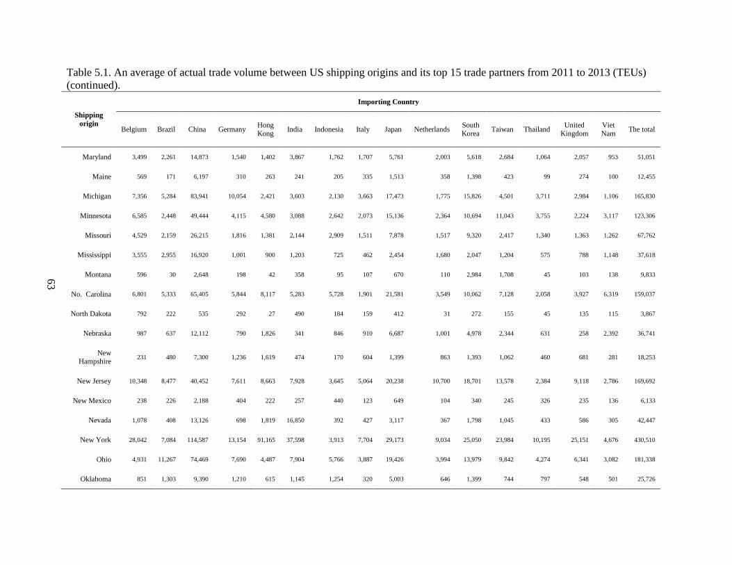
63
Table 5.1. An average of actual trade volume between US shipping origins and its top 15 trade partners from 2011 to 2013 (TEUs)
(continued).
Shipping
origin
Importing Country
Belgium Brazil China Germany Hong Kong
India Indonesia Italy Japan Netherlands South Korea
Taiwan Thailand United
Kingdom Viet Nam
The total
Maryland 3,499 2,261 14,873 1,540 1,402 3,867 1,762 1,707 5,761 2,003 5,618 2,684 1,064 2,057 953 51,051
Maine 569 171 6,197 310 263 241 205 335 1,513 358 1,398 423 99 274 100 12,455
Michigan 7,356 5,284 83,941 10,054 2,421 3,603 2,130 3,663 17,473 1,775 15,826 4,501 3,711 2,984 1,106 165,830
Minnesota 6,585 2,448 49,444 4,115 4,580 3,088 2,642 2,073 15,136 2,364 10,694 11,043 3,755 2,224 3,117 123,306
Missouri 4,529 2,159 26,215 1,816 1,381 2,144 2,909 1,511 7,878 1,517 9,320 2,417 1,340 1,363 1,262 67,762
Mississippi 3,555 2,955 16,920 1,001 900 1,203 725 462 2,454 1,680 2,047 1,204 575 788 1,148 37,618
Montana 596 30 2,648 198 42 358 95 107 670 110 2,984 1,708 45 103 138 9,833
No. Carolina 6,801 5,333 65,405 5,844 8,117 5,283 5,728 1,901 21,581 3,549 10,062 7,128 2,058 3,927 6,319 159,037
North Dakota 792 222 535 292 27 490 184 159 412 31 272 155 45 135 115 3,867
Nebraska 987 637 12,112 790 1,826 341 846 910 6,687 1,001 4,978 2,344 631 258 2,392 36,741
New Hampshire
231 480 7,300 1,236 1,619 474 170 604 1,399 863 1,393 1,062 460 681 281 18,253
New Jersey 10,348 8,477 40,452 7,611 8,663 7,928 3,645 5,064 20,238 10,700 18,701 13,578 2,384 9,118 2,786 169,692
New Mexico 238 226 2,188 404 222 257 440 123 649 104 340 245 326 235 136 6,133
Nevada 1,078 408 13,126 698 1,819 16,850 392 427 3,117 367 1,798 1,045 433 586 305 42,447
New York 28,042 7,084 114,587 13,154 91,165 37,598 3,913 7,704 29,173 9,034 25,050 23,984 10,195 25,151 4,676 430,510
Ohio 4,931 11,267 74,469 7,690 4,487 7,904 5,766 3,887 19,426 3,994 13,979 9,842 4,274 6,341 3,082 181,338
Oklahoma 851 1,303 9,390 1,210 615 1,145 1,254 320 5,003 646 1,399 744 797 548 501 25,726

64
Table 5.1. An average of actual trade volume between US shipping origins and its top 15 trade partners from 2011 to 2013 (TEUs)
(continued).
Shipping
origin
Importing Country
Belgium Brazil China Germany Hong
Kong India Indonesia Italy Japan Netherlands
South
Korea Taiwan Thailand
United
Kingdom
Viet
Nam The total
Oregon 1,100 2,840 76,674 2,433 3,915 2,291 5,271 994 20,216 1,142 16,607 18,267 2,053 1,322 17,771 172,897
Pennsylvania 9,963 9,306 77,834 9,833 4,720 8,326 4,190 5,156 21,773 8,771 16,594 12,320 2,180 6,470 2,114 199,551
Rhode Island 289 103 2,195 1,168 354 209 58 783 588 126 473 1,611 324 295 216 8,793
So. Carolina 4,427 4,684 92,529 20,203 2,849 7,229 2,160 2,037 8,443 2,115 7,838 6,377 1,809 5,749 3,393 171,842
South Dakota 367 129 1,637 134 181 29 127 71 641 20 280 165 81 75 134 4,072
Tennessee 11,897 5,054 53,205 4,229 3,622 4,089 5,121 2,838 23,216 4,965 10,176 7,681 2,475 3,725 5,363 147,655
Texas 43,466 73,267 266,972 15,462 16,484 33,030 25,297 9,858 60,415 48,736 121,499 89,184 17,294 16,877 22,870 860,711
Utah 2,099 750 21,151 1,490 46,453 10,018 1,055 1,291 6,803 948 4,217 13,606 8,900 19,561 678 139,019
Virginia 4,086 4,919 46,860 4,767 2,397 4,266 6,597 1,955 6,553 2,373 5,309 10,500 1,424 4,419 4,465 110,890
Vermont 244 44 15,486 312 2,990 181 208 161 1,899 205 2,317 3,703 705 221 211 28,887
Washington 4,035 7,973 350,174 9,967 24,053 21,537 48,490 1,977 95,803 5,407 49,177 37,272 10,544 8,813 9,459 684,682
Wisconsin 3,855 3,669 38,161 4,258 2,923 5,577 2,086 2,353 10,758 1,988 6,601 4,695 2,687 2,674 2,358 94,642
West Virginia 3,052 4,482 15,973 1,700 774 8,839 294 4,912 6,519 4,041 6,305 1,055 363 1,909 363 60,581
Wyoming 87 837 241 13 13 62 2,169 3 633 221 679 953 442 93 383 6,828
Total 271840 303954 2726751 258174 389609 333248 213618 116547 814673 201060 649634 590242 142542 209061 192100

65
Figure 5.1 shows official regions and divisions of the United States and it is used for
measurement of trade volumes and flows by US regions and divisions. The northeast region of
the United States produces 15.02% of the total US exports, the Midwest region of the United
States exports 16.43% of the total US exports, the South region of the United States produces
35.73% of the total US exports, and the West region of the United States exports 32.83% of the
total US exports. On the other hand, approximately, 77.15% of the total US containerized
shipments are imported by countries in Asia, while 18.75% and 4.1% of the total US
containerized shipments are imported by countries in Europe and South America, respectively.
Figure 5.1. Official regions of the United States. Source: US Census (2015).
5.1.2. Trade Volume of Containerized Shipments for US Imports
Table 5.2 shows the average trade volume between US shipping destinations and its top
15 trade partners for US imports from 2011 to 2013. The total quantities of containerized

66
shipments for US imports are over 14.4 million TEUs. California is the largest consumption state
for containerized shipments in the United States. California imports approximately 3.7 million
TEUs, accounting for 25.63% of the total US imports. Texas and New York are the second and
third largest consumption states. They import approximately 1.3 million TEUs and 1 million
TEUs, respectively, which account for 9.39% and 7.43% of the total US imports. Illinois and
New Jersey are the fourth and fifth largest consumption states, respectively. Those five states
account for 53% of the total US imports.
China, as the largest exporting country, exports more than 8.6 million TEUs of
containerized shipments, accounting for 59.77% of the total US imports. South Korea and Japan
are the second and third largest exporting countries to the US, which imports more than 695,000
TEUs and 619,000 TEUs, respectively, accounting for 4.82% and 4.29% of the total US imports.
Vietnam and Germany are the fourth and fifth largest exporting countries to the US, respectively.
Those five exporting countries account for 76.33% of the total US imports. The northeast region
of the United States consumes 19.16 of the total US imports. The Midwest region of the United
States imports 16.94% of the total US imports, the south region of the United States consumes
32.7% of the total US imports, and the west region of the United States imports 31.2% of the
total US imports. Approximately 83.99% of the total containerized shipments for US imports are
from countries in Asia, while 14.08% and 1.94% of the total containerized shipments for US
imports are from countries in Europe and South America, respectively.

67
Table 5.2. An average of actual trade volume between US shipping destinations and its top 15 trade partners from 2011 to 2013 (TEUs)
Shipping
destination
Exporting Country
Belgium Brazil China Germany Hong Kong
India Indonesia Italy Japan Netherlands South Korea
Taiwan Thailand United
Kingdom Viet Nam
Total
Alabama 1166 15898 40452 14102 837 986 1458 3476 5437 976 44770 1827 644 640 3831 136500
Arkansas 335 242 43350 1780 844 2518 521 905 610 555 1482 1644 1045 299 1004 57135
Arizona 382 943 52661 3086 7463 1784 1233 1794 6617 2992 3366 6748 3188 1548 1626 95432
California 7788 24696 2604119 60280 86888 34120 79124 28665 183998 12314 148000 148506 114294 12127 154326 3699245
Colorado 669 531 39427 3024 3442 4307 530 2683 945 1536 3055 2793 1043 903 4052 68940
Connecticut 2808 2995 56027 7894 3641 2302 1574 5116 4529 13820 1947 3705 1380 6482 3773 117991
District of
Columbia 43 78 396 235 61 177 9 241 161 367 136 13 30 131 37 2115
Delaware 14977 2524 10481 1589 435 1271 129 823 473 3197 178 415 46 9042 195 45775
Florida 4713 31140 237016 10287 20842 9670 8852 15265 18195 12087 14987 13716 10028 7279 27180 441257
Georgia 6208 7162 331080 61604 16111 15578 13267 13115 20444 8045 68015 13639 16616 6925 20686 618495
Iowa 465 1160 26230 3173 531 1682 224 3040 1768 737 1552 2439 557 370 1034 44962
Idaho 28 77 15925 388 548 119 278 3216 1979 348 4285 9167 71 77 574 37081
Illinois 8770 6823 526970 25575 11878 13167 11264 15860 38875 33159 63928 29327 13780 6844 21873 828092
Indiana 2170 4214 126175 11163 2746 4352 3093 6540 23039 4356 3744 11361 7320 4092 8456 222822
Kansas 1396 1532 44095 3955 1983 866 2201 2584 1112 781 2591 16580 794 1567 7136 89173
Kentucky 4458 2667 132175 9294 6769 8587 7670 14587 20858 2620 8161 19947 7598 3665 11009 260064
Louisiana 17276 18129 21214 3223 1097 4447 8984 2340 1490 5224 6888 1104 1675 2932 2584 98608
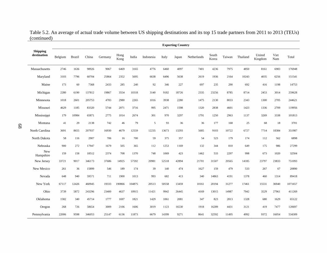
68
Table 5.2. An average of actual trade volume between US shipping destinations and its top 15 trade partners from 2011 to 2013 (TEUs)
(continued)
Shipping
destination
Exporting Country
Belgium Brazil China Germany Hong Kong
India Indonesia Italy Japan Netherlands South Korea
Taiwan Thailand United
Kingdom Viet Nam
Total
Massachusetts 2746 1636 98926 9067 6469 3165 4776 6460 4097 7401 4236 7975 4850 8161 6983 176948
Maryland 3103 7796 60704 25864 2352 5695 6638 6496 5638 2619 1936 2164 10243 4035 6256 151541
Maine 173 60 7368 2433 285 240 92 346 227 697 235 290 692 416 1198 14753
Michigan 2280 6190 137812 19867 3554 10318 3140 9182 18726 2335 23256 8785 8714 2453 3014 259628
Minnesota 1018 2601 205753 4783 2980 2265 1016 3938 2280 1475 2130 8033 2343 1300 2705 244621
Missouri 4629 1185 83320 5744 2071 3716 995 2471 1598 1320 2838 4601 1423 1336 2709 119956
Mississippi 179 10984 65871 2775 1014 2674 301 970 3297 1791 1250 2963 1137 3269 3338 101813
Montana 41 29 2138 742 46 79 5 93 36 36 177 168 25 68 18 3701
North Carolina 3691 8655 207937 16930 4679 12559 12235 13673 13293 5685 9103 10722 6727 7714 18384 351987
North Dakota 58 116 2907 706 16 700 59 375 357 54 523 179 174 112 562 6898
Nebraska 900 272 17947 1679 505 365 112 1253 1169 132 344 810 649 175 986 27299
New
Hampshire 159 158 18512 2374 708 1370 748 1069 423 1462 533 2297 998 673 1020 32504
New Jersey 33721 9017 346173 37686 14925 57592 20981 52518 42894 21701 31507 20565 14185 23797 23833 751093
New Mexico 261 36 15899 546 189 174 39 140 474 1627 159 479 533 267 67 20890
Nevada 648 940 59571 711 1900 1013 993 682 413 340 14863 4191 1378 460 1314 89418
New York 67117 12426 460945 19333 190866 104875 20513 50558 13459 10161 20194 31277 17461 15531 36940 1071657
Ohio 3739 5872 243296 23400 4637 10915 11421 9942 26445 4169 13015 14987 7942 3529 27961 411269
Oklahoma 1582 340 45714 1777 1697 1821 1429 1061 2081 347 823 2813 1328 680 1629 65122
Oregon 268 726 58654 3009 2106 1606 3019 1123 16530 1918 16289 4431 3121 419 7477 120697
Pennsylvania 22006 9598 346053 25147 6136 11873 6679 14399 9271 8641 32592 11495 4992 9372 16054 534309

69
Table 5.2. An average of actual trade volume between US shipping destinations and its top 15 trade partners from 2011 to 2013 (TEUs)
(continued)
Shipping
destination
Exporting Country
Belgium Brazil China Germany Hong Kong
India Indonesia Italy Japan Netherlands South Korea
Taiwan Thailand United
Kingdom Viet Nam
Total
Rhode Island 1130 655 25101 16676 584 1467 209 819 633 3049 358 748 1320 2170 429 55348
South Carolina 5738 6267 111239 34886 1722 8713 14398 10882 7921 7435 4595 4846 6770 4445 10208 240064
South Dakota 33 1055 2581 137 68 47 9 218 71 48 103 252 107 30 97 4857
Tennessee 11893 4082 435571 13076 4578 14862 17810 7598 39750 2961 5375 10632 9604 4477 28981 611252
Texas 19538 57407 825238 35917 18671 51829 17627 30721 32085 23693 99929 43821 38308 16894 42944 1354621
Utah 143 837 34627 945 2106 671 427 791 632 279 689 3768 362 269 1183 47728
Virginia 2611 5053 90504 9065 2281 9405 9528 7000 8726 2324 2138 3333 2730 3228 10185 168112
Vermont 43 69 5546 555 188 672 510 417 228 106 414 352 78 213 783 10174
Washington 1547 2914 179038 4168 5179 3616 5404 5484 28719 4489 25037 28346 7079 5441 10570 317032
Wisconsin 1221 1230 117034 6395 4192 6799 6770 7104 3560 1839 3760 6723 1376 1018 16965 185985
West Virginia 484 253 5289 896 101 1347 114 542 4203 125 122 434 82 158 922 15071
Wyoming 18 6 2260 164 48 133 12 22 37 23 64 53 9 80 47 2977
Total 266367 279279 8627320 548105 452968 438508 308421 368599 619803 223395 695674 525462 336851 187116 555145

70
5.1.3. Trade Volume and Total Toll Revenue of Containerized Shipments at the Panama
Canal
Table 5.3 shows the trade volume of containerized shipments between the United States
and its trade partners through the Panama Canal (PNC), and it also contains the total toll revenue
at the PNC. Prior to the Panama Canal Expansion (PCE), more than 2 million TEUs of
containerized shipments are exported from US export ports to import ports in other countries
through the PNC, while more than 4.5 million TEUs of containerized shipments are imported
from export ports in other countries to US import ports through the PNC. In other words, 27% of
the total US exports and 32% of the total US imports are shipped via the PNC.
The total toll revenue at the PNC is about $488 million dollars, with existing delays
costing $6.34 per TEU and a toll rate at $74 per TEU. These were factored into the base model.
After the PCE with a 50% reduced delay cost and without delay costs at the canal, it is expected
that more than 2.6 million TEUs of containerized shipments will be exported from US export
ports to import ports in other countries through the PNC, while more than 4.9 million TEUs of
containerized shipments will be imported from export ports in other countries to US import ports
through the PNC. In other words, 36% of the total US exports and 34% of the total US imports
are anticipated to be shipped via the PNC.
The total toll revenue at the PNC is about $563 million dollars with a 50% reduced delay
cost ($3.17 per TEU) in Model 1 and the same without delay cost at the canal with same toll rate
in Model 2. Since traffic volume at the PNC increases by 31% for US exports and 8% for US
imports, respectively in Models 1 and 2, the total toll revenue at the PNC increases by more than
15%. After the PCE and US port expansion (50% increased capacity) with 50% reduced delay
cost (Model 3) and no delay cost (Model 4) at the Canal, more than 3 million TEUs of

71
containerized shipments will be exported from US export ports to import ports in other countries
through the PNC, while more than 6.2 million TEUs of containerized shipments are expected to
be imported from export ports in other countries to US import ports through the PNC. In other
words, 41% of the total US exports and 43% of the total US imports will be shipped via the PNC.
Table 5.3. Trade volume and the total toll revenue of containerized shipments at the Panama
Canal.
Base Model Model 1 Model 2 Model 3 Model 4
Trade
Volume
(TEUs) at
the PNC
US
Export 2,021,409 2,640,077 2,648,310 3,046,233 3,046,233
US
Import 4,584,475 4,964,146 4,964,146 6,202,617 6,202,618
Trade
Volume (%)
at the PNC
US
Export 27% 36% (31%↑) 36% (31%↑) 41% (51%↑) 41% (51%↑)
US
Import 32% 34% (8%↑) 34% (8%↑) 43% (35%↑) 43% (35%↑)
Toll Revenue
(US $) at the
PNC
$488,835,416 $562,712,502 $563,321,744 $684,414,900 $684,414,974
% Change in
Toll Revenue 15.11% ↑ 15.24% ↑ 40% ↑ 40% ↑
The total toll revenue at the PNC is about $684 million dollars with both 50% reduced
delay cost ($3.17 per TEU) and no delay cost at the canal with same toll rate in Models 3 and 4.
Since trade volume at the PNC increases by 51% for US exports and 35% for US imports
respectively, the total toll revenue at the PNC increases by 40%.Thus, after the Panama Canal is
expanded, more containerized shipments for US export and import will be moved through the
PNC because of the lower ocean freight rates associated with vessel size for the hauling of
containerized shipments. For instance, ocean freight rate between the Port of Shanghai in China
and the port of Houston, Texas in the United States by Panamax vessel with current capacity at

72
the PNC is $3,101 per TEU, excluding port handling charges at export and import ports, delay
costs and the toll rate at the canal. However, the ocean freight rate on the same route by a New
Panamax vessel with an unlimited capacity after the expanded PNC is finished is $1,972 per
TEU. The ocean freight rate on this route decreases to $1,129 when the Panama Canal is
expanded. Therefore, the PCE affects trade volume and the total toll revenue at the PNC. If the
Panama Canal and US Ports are expanded, even more containerized shipments for US exports
and imports are shipped through the PNC, because larger port capacity allows US ports in the
East and the Gulf Coast to handle more shipments for US exports and imports. Although the
Panama Canal and US port expansion have very significant impacts on trade volume and the
total toll revenue at the canal, delay costs at the canal do not affect trade volume and the total toll
revenue at the canal, mainly because delay costs at the PNC accounts for a small portion of the
total transportation costs.
5.1.4. Trade Volume and Flows at Container Ports in the United States
Table 5.4 shows trade volume and flows at US major container ports. In Table 5.4,
coastal regions in the United States are divided into 6 regions: (1) Pacific Northwest (PNW)
including major US container ports in Washington and Oregon, (2) Los Angeles and Long Beach
(LA/LB) including major container ports in California, (3) the West side of the Gulf of Mexico
(West Gulf) including major US container ports in Texas, (4) the East side of the Gulf of Mexico
(East Gulf) including major US container ports in Louisiana, Mississippi, Alabama, the South
side of Georgia, and the West side of Florida, (5) the South Atlantic including major US
container ports in the East side of Florida, the Southeast side of Georgia, South Carolina and
North Carolina, and (6) the Mid-Atlantic including major US container ports in Virginia,
Maryland, Delaware, Pennsylvania, New York and New Jersey. Since none of the container

73
ports are ranked as the top 15 US container ports in the North Atlantic, this study is focused on
six coastal regions in the United States.
Table 5.4. Trade volume and flows at container ports in the United States.
Base Model Model 2 Model 4
Coastal
Region Port
US Export
(TEUs)
US
Import
(TEUs)
Total
(TEUs)
Port
Usage
(%)
US
Export
(TEUs)
US
Import
(TEUs)
Total
(TEUs)
Port
Usage
(%)
US
Export
(TEUs)
US Import
(TEUs)
Total
(TEUs)
Port
Usage
(%)
PNW
Seattle, WA 663493 0 663493 50.90 257771 0 257771 19.78 0 0 0 0
Tacoma,
WA 259993 730945 990938 100 505529 485409 990938 100 742653 417232 1159885 78.03
Portland,
OR 0 0 0 0 156117 0 156117 100 172897 61279 234176 100
LA/LB
Los
Angeles,
CA
2560654 5402679 7963333 100 2203826 5471672 7675498 96.39 1543766 4240098 5783864 48.42
Long
Beach, CA 0 203128 203128 2.68 0 0 0 0 0 0 0 0
West
Gulf
Freeport,
TX 52704 0 52704 100 0 52704 52704 100 0 79056 79056 100
Houston,
TX 0 1475997 1475997 100 450117 1025880 1475997 100 884305 1329691 2213996 100
East
Gulf
Gulfport,
MS 70939 103179 174118 100 0 174118 174118 100 16556 244621 261177 100
Mobile, AL 87997 41201 129198 100 0 129198 129198 100 0 193797 193797 100
New
Orleans, LA 299518 0 299518 100 78438 221080 299518 100 22406 426871 449277 100
South
Atlantic
Charleston,
SC 117233 136500 253733 21.76 160254 336851 497105 42.63 117233 136500 253733 14.51
Miami, FL 159217 441257 600474 82.19 285807 444823 730630 100 159217 936728 1095945 100
Savannah,
GA 889616 1389539 2279155 100 963677 1315478 2279155 100 1650949 1767784 3418733 100
Mid-
Atlantic
New York,
NY 1655519 3844481 5500000 100 1677706 3822294 5500000 100 1304558 3632934 4937492 59.85
Norfolk,
VA 596165 664106 1260271 77.45 673806 953505 1627311 100 798508 966421 1764929 72.3
Container ports in PNW handle approximately 923,000 TEUs for US exports and
730,000 TEUs for US imports and meet 67.51% of their current capacities in the base model.
Container ports in PNW handle more shipments for US exports than imports. While PNW
continues to handle more shipments for US exports than imports, the total containerized
74
shipments at PNW decrease by 15.09% when the PNC is expanded and decrease by 15.74%
when the PNC and its port capacity are expanded. Unlike PNW, container ports in LA/LB handle
approximately 2.5 million TEUs for US exports and 5.6 million TEUs for US imports and meet
52.53% of their current capacities in the base model. Container ports in LA/LB handle more
shipments for US imports than exports. While LA/LB continues to handle more shipments for
US imports than exports, the total containerized shipments at LA/LB decreases by 6.01% when
the PNC is expanded and decreases by 29.18% when the PNC and US port capacities are
expanded.
More than 1.5 million TEUs are handled by container ports in the West Gulf, which
meets 100% of current port capacities in the base model. In this area, container ports handle the
majority of their shipments for US imports about 96.55% of the total throughput at the West Gulf
is come from other countries. However, when the PNC is expended, 29.44% of the total
throughput at the West Gulf is shipped out and 70.56% is from other countries, while container
ports in the West Gulf fully use their current capacities. If ports in the West Gulf expand their
capacity by 50% of their current capacity with the PCE, the total throughput at the West Gulf
increases by 50%, which means ports in that area fully meet their new capacities as well. About
38.56% and 61.44% of the total throughput at the West Gulf are US exports and imports,
respectively.
In the East Gulf, 76.05% of the total throughput at the East Gulf is US exports, while
23.95% is US imports. Container ports in West Gulf handle more shipments for US exports than
import. They meet 100% of their current capacities in the base model. On the other hand, 86.99%
of the total throughput at the West Gulf is from other countries and 13.01% is shipped out after
the PCE. They meet 100% of their current capacities in Model 2 as well. If ports in that area

75
expanded their capacities with the PCE, they would handle 95.69% of the total throughput as
shipments for US imports, while they would fully use their expanded capacities.
Under the current status of port facilities in the South Atlantic, about 3.1 million TEUs
are shipped through these ports. About 62.79% of the total throughput in the South Atlantic is
from other countries and 37.21% is shipped out. Container ports in the South Atlantic meet 75.03%
of their current capacities in the base model. Since quantities of containerized shipments in the
South Atlantic increase after the PCE, container ports in the South Atlantic handle 11.92% more
than prior to the changes. Usage of ports increases to 83.98% from 75.03% of current capacity in
Model 2. In the South Atlantic, if ports and the PNC are expanded, the total throughput increases
to 4.7 million TEUs from 3.1 million TEUs, which is 52.18% increase. Usage of ports is 76.13%
of the new capacity.
Container ports in the Mid-Atlantic handle approximately 2.2 million TEUs for US
exports and 4.5 million TEUs for US imports and meet 94.85% of their current capacities in the
base model. Container ports in the Mid-Atlantic handle more shipments for US exports than
imports. While the Mid-Atlantic continues to handle more shipments for US exports than imports,
the total containerized shipments at the Mid-Atlantic increase by 5.43% and meets current port
capacity when the PNC is expanded. However, the total containerized shipments at the Mid-
Atlantic decreases by 0.86% and meets 62.69% of a new port capacity when the PNC and ports
are expanded together.
Major container ports in the United States are characterized under given alternative
scenarios in this section. Prior to the Panama Canal Expansion, all container ports by coastal
regions in the United States use more than 50% of their current capacities. Container ports in the
West Coast of the US use approximately 55%, container ports in the Gulf of Mexico use 100%,

76
and container ports in the East Coast use about 88% of their current capacities. Although all
container ports by coastal regions in the United States continue to use more than 50% of their
current capacities, usage of ports in the West Coast decreases by 4%, as the total throughput
decreases by 6%, while usage of ports in the East Coast increases by 7%, as the total throughput
increases by 5%, and usage of ports and the total throughput in the Gulf Coast remains the same
as before the PCE.
Thus, the Panama Canal Expansion will have significant impacts on the total throughput
at ports in the United States. For instance, ports in the West Coast loses total throughput, but
ports in the Gulf and East Coast have the same or more shipments after the PCE. Furthermore,
ports in the Gulf Coast and East Coast may need to be expanded, because usage of these ports
increase to 100% and 94%, respectively, after the PCE.
On the other hand, if the Panama Canal and major US container ports are expanded,
usage of ports in the West Coast decreases by 28%, as the total throughput decreases by 29%,
and usage of ports in the East Coast decreases by 20%, as the total throughput decreases by 1%.
Since ports in the Gulf meet 100% of their capacities in all models, usage of ports in the Gulf
Coast remains the same as the base case, while the total throughput increases by 50%. Under this
new trade circumstance, in the United States, ports in the Gulf Coast need to be expanded by 50%
of their current capacities and by even more than 50% since ports in the Gulf Coast fully use
their new capacities. Ports in the East Coast also need to be expanded to handle more
containerized shipments; however, it is not necessary to increase its capacity as much as 50% of
their current capacities, because ports in the East Coast use 68% of their new capacities under the
current volume of containerized shipments. However, ports in the West Coast should not expand

77
their capacities because they will only use 27% of their new capacities if the PCE and ports are
expanded.
5.1.5. Domestic Trade Volume and Flows of Containerized Shipments in the United States
Table 5.5 shows domestic trade volume and flows of containerized shipments by trucks
in the United States. Prior to the PCE, approximately 1.2 million TEUs of containerized
shipments for US exports are transited from shipping origins in California to the ports of Los
Angeles or Long Beach, and 3.7 million TEUs of containerized shipments for US imports are
shipped from the ports of Los Angeles or Long Beach to shipping destinations in California by
truck. In New York and its neighbor states such as New Jersey or Connecticut, more than
430,000 TEUs, 169,000 TEUs, and 71,000 TEUs of containerized shipments for US exports are
delivered to the port of New York from their shipping destinations by truck, respectively.
Shipping destinations in New York, New Jersey, and Connecticut receive about 1 million TEUs,
751,000 TEUs, and 117,000 TEUs of containerized shipments for US imports from the port of
New York by truck, respectively. Washington and Oregon are shipped more than 684,000 TEUs
and 172,000 TEUs of containerized shipments for US exports from their shipping origins to the
ports of Seattle or Tacoma by truck and shipping destinations in Washington and Oregon receive
more than 317,000 TEUs and 120,000 TEUs of containerized shipments for US imports from the
ports of Seattle or Tacoma by truck, respectively. Shipping origin in Florida ships out 159,000
TEUs of containerized shipments for US exports to the port of Miami and 441,000 TEUs of
containerized shipments are moved from the port of Miami to Florida by truck. In Virginia,
71,000 TEUs of containerized shipments for US exports are transited from its shipping origin to
the port of Norfolk, while its shipping destination receives about 118,000 TEUs from the port of

78
Norfolk by truck. Those eight shipping origins and destinations are connected with five container
ports in the United States in the base model.
Table 5.5. Domestic trade volume and flows of containerized shipments by truck in the United
States (TEUs).
US Export US Import
Shipping
origin Container Port
Volume
(TEUs) Container Port
Shipping
destination
Volume
(TEUs)
Base
Model
California LA/LB, CA 1,197,546 LA/LB, CA California 3,699,245
New York New York, NY 430,510 New York, NY New York 1,071,657
Washington Seattle/Tacoma,
WA 684,682
Seattle/Tacoma,
WA Washington 317,032
New Jersey New York, NY 169,692 New York, NY New Jersey 751,093
Florida Miami, FL 159,217 Miami, FL Florida 441,257
Oregon Seattle/Tacoma,
WA 172,897
Seattle/Tacoma,
WA Oregon 120,697
Virginia Norfolk, VA 110,890 Norfolk, VA Virginia 168,112
Connecticut New York, NY 71,173 New York, NY Connecticut 117,991
Model
2
California LA/LB, CA 1,197,546 LA/LB, CA California 3,699,245
New York New York, NY 430,510 New York, NY New York 1,071,657
Washington Seattle/Tacoma,
WA 684,682
Seattle/Tacoma,
WA Washington 317,032
New Jersey New York, NY 169,692 New York, NY New Jersey 751,093
Florida Miami, FL 159,217 Miami, FL Florida 441,257
Oregon
Seattle/Tacoma,
WA 16,780 Seattle/Tacoma,
WA Oregon 120,697
Portland, OR 156,117
Virginia Norfolk, VA 110,890 Norfolk, VA Virginia 168,112
Connecticut New York, NY 71,173 New York, NY Connecticut 117,991
North
Carolina Charleston, SC 43,021 Charleston, SC
North
Carolina 3,918
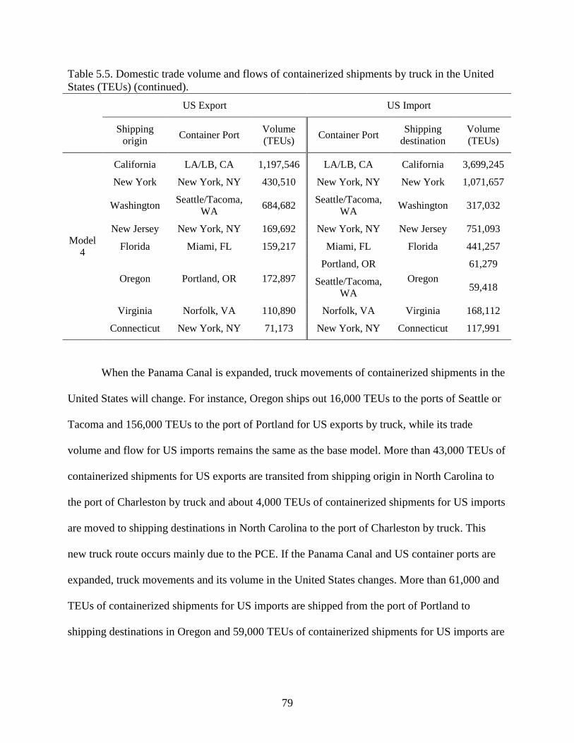
79
Table 5.5. Domestic trade volume and flows of containerized shipments by truck in the United
States (TEUs) (continued).
US Export US Import
Shipping
origin Container Port
Volume
(TEUs) Container Port
Shipping
destination
Volume
(TEUs)
Model
4
California LA/LB, CA 1,197,546 LA/LB, CA California 3,699,245
New York New York, NY 430,510 New York, NY New York 1,071,657
Washington Seattle/Tacoma,
WA 684,682
Seattle/Tacoma,
WA Washington 317,032
New Jersey New York, NY 169,692 New York, NY New Jersey 751,093
Florida Miami, FL 159,217 Miami, FL Florida 441,257
Oregon Portland, OR 172,897
Portland, OR
Oregon
61,279
Seattle/Tacoma,
WA 59,418
Virginia Norfolk, VA 110,890 Norfolk, VA Virginia 168,112
Connecticut New York, NY 71,173 New York, NY Connecticut 117,991
When the Panama Canal is expanded, truck movements of containerized shipments in the
United States will change. For instance, Oregon ships out 16,000 TEUs to the ports of Seattle or
Tacoma and 156,000 TEUs to the port of Portland for US exports by truck, while its trade
volume and flow for US imports remains the same as the base model. More than 43,000 TEUs of
containerized shipments for US exports are transited from shipping origin in North Carolina to
the port of Charleston by truck and about 4,000 TEUs of containerized shipments for US imports
are moved to shipping destinations in North Carolina to the port of Charleston by truck. This
new truck route occurs mainly due to the PCE. If the Panama Canal and US container ports are
expanded, truck movements and its volume in the United States changes. More than 61,000 and
TEUs of containerized shipments for US imports are shipped from the port of Portland to
shipping destinations in Oregon and 59,000 TEUs of containerized shipments for US imports are

80
transited from the ports of Seattle or Tacoma to shipping destinations in Oregon by truck. All
other truck movements and volumes remain the same as the base case.
Table 5.6 shows domestic trade volume and flows of containerized shipments by truck-
barge combinations in the United States. Under current trade movement of containerized
shipments in the United States, shipping origins in Arkansas transits 33,000 TEUs of
containerized shipments for US exports to the port of Freeport via the river port of Little Rock,
Arkansas, by truck-barge combination and 57,000 TEUs of containerized shipments for US
imports are shipped from the port of Houston to shipping destinations in Arkansas via the river
port of Little Rock, Arkansas, by a truck-barge combination.
Illinois ships out more than 35,000 TEUs, 84,000 TEUs, and 19,000 TEUs of
containerized shipments for US exports to the ports of Mobile, New Orleans, and Freeport via
the river port of Chicago, Illinois, by a truck-barge combination. Shipping destinations in Illinois
receive 728,000 TEUs from the port of Houston and 99,000 TEUs from the port of Gulfport via
the river port of Chicago, Illinois, by a truck-barge combination for US imports.
More than 52,000 TEUs and 70,000 TEUs of containerized shipments for US exports are
shipped to the ports of Mobile and the Gulfport via the river port of Minneapolis, Minnesota,
from shipping origin in Minnesota, respectively and about 4,000 TEUs of containerized
shipments of US imports are transited from the port of the Gulfport to Minnesota via the river
port of Minneapolis, Minnesota, by a truck-barge combination.
In Missouri, more than 67,000 TEUs are moved to the port of New Orleans from its
shipping origin via St. Louis, Missouri, for US exports and 78,000 TEUs and 41,000 TEUs of
containerized shipments for the U.S import are transited from the ports of Houston and Mobile to
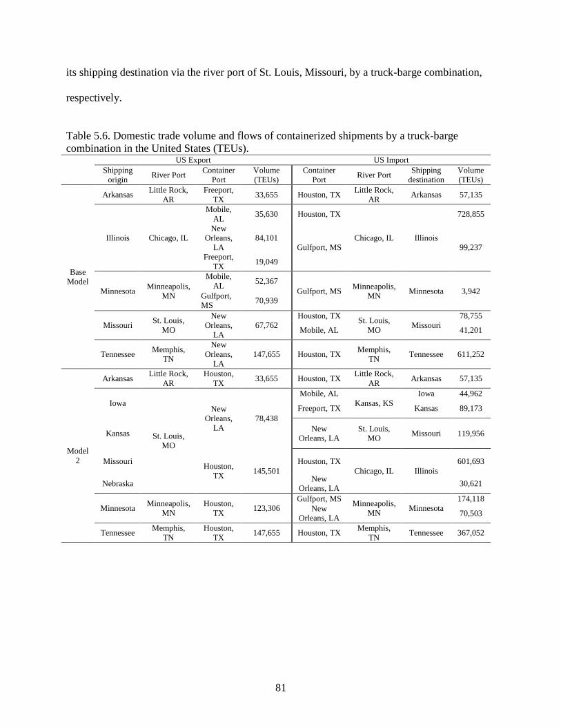
81
its shipping destination via the river port of St. Louis, Missouri, by a truck-barge combination,
respectively.
Table 5.6. Domestic trade volume and flows of containerized shipments by a truck-barge
combination in the United States (TEUs).
US Export US Import
Shipping
origin River Port
Container
Port
Volume
(TEUs)
Container
Port River Port
Shipping
destination
Volume
(TEUs)
Base
Model
Arkansas Little Rock,
AR
Freeport,
TX 33,655 Houston, TX
Little Rock,
AR Arkansas 57,135
Illinois Chicago, IL
Mobile,
AL 35,630 Houston, TX
Chicago, IL Illinois
728,855
New
Orleans,
LA
84,101
Gulfport, MS 99,237
Freeport,
TX 19,049
Minnesota Minneapolis,
MN
Mobile,
AL 52,367
Gulfport, MS Minneapolis,
MN Minnesota 3,942
Gulfport,
MS 70,939
Missouri St. Louis,
MO
New
Orleans,
LA
67,762
Houston, TX St. Louis,
MO Missouri
78,755
Mobile, AL 41,201
Tennessee Memphis,
TN
New
Orleans,
LA
147,655 Houston, TX Memphis,
TN Tennessee 611,252
Model
2
Arkansas Little Rock,
AR
Houston,
TX 33,655 Houston, TX
Little Rock,
AR Arkansas 57,135
Iowa
St. Louis,
MO
New
Orleans,
LA
78,438
Mobile, AL
Kansas, KS
Iowa 44,962
Freeport, TX Kansas 89,173
Kansas New
Orleans, LA
St. Louis,
MO Missouri 119,956
Missouri Houston,
TX 145,501
Houston, TX
Chicago, IL Illinois
601,693
Nebraska New
Orleans, LA 30,621
Minnesota Minneapolis,
MN
Houston,
TX 123,306
Gulfport, MS Minneapolis,
MN Minnesota
174,118
New
Orleans, LA 70,503
Tennessee Memphis,
TN
Houston,
TX 147,655 Houston, TX
Memphis,
TN Tennessee 367,052
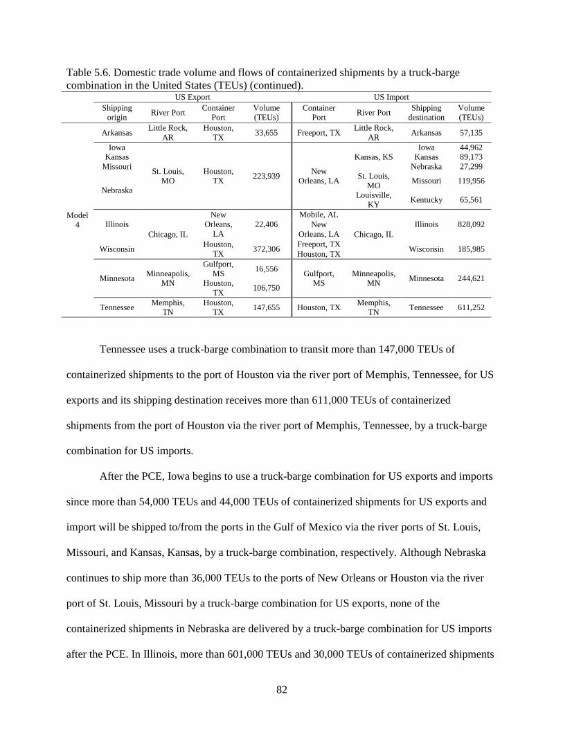
82
Table 5.6. Domestic trade volume and flows of containerized shipments by a truck-barge
combination in the United States (TEUs) (continued).
US Export US Import
Shipping
origin River Port
Container
Port
Volume
(TEUs)
Container
Port River Port
Shipping
destination
Volume
(TEUs)
Model
4
Arkansas Little Rock,
AR
Houston,
TX 33,655 Freeport, TX
Little Rock,
AR Arkansas 57,135
Iowa
St. Louis,
MO
Houston,
TX 223,939
New
Orleans, LA
Kansas, KS
Iowa 44,962
Kansas Kansas 89,173
Missouri Nebraska 27,299
Nebraska
St. Louis,
MO Missouri 119,956
Louisville,
KY Kentucky 65,561
Illinois
Chicago, IL
New
Orleans,
LA
22,406
Mobile, AL
Chicago, IL
Illinois 828,092 New
Orleans, LA
Wisconsin Houston,
TX 372,306
Freeport, TX Wisconsin 185,985
Houston, TX
Minnesota Minneapolis,
MN
Gulfport,
MS 16,556
Gulfport,
MS
Minneapolis,
MN Minnesota 244,621
Houston,
TX 106,750
Tennessee Memphis,
TN
Houston,
TX 147,655 Houston, TX
Memphis,
TN Tennessee 611,252
Tennessee uses a truck-barge combination to transit more than 147,000 TEUs of
containerized shipments to the port of Houston via the river port of Memphis, Tennessee, for US
exports and its shipping destination receives more than 611,000 TEUs of containerized
shipments from the port of Houston via the river port of Memphis, Tennessee, by a truck-barge
combination for US imports.
After the PCE, Iowa begins to use a truck-barge combination for US exports and imports
since more than 54,000 TEUs and 44,000 TEUs of containerized shipments for US exports and
import will be shipped to/from the ports in the Gulf of Mexico via the river ports of St. Louis,
Missouri, and Kansas, Kansas, by a truck-barge combination, respectively. Although Nebraska
continues to ship more than 36,000 TEUs to the ports of New Orleans or Houston via the river
port of St. Louis, Missouri by a truck-barge combination for US exports, none of the
containerized shipments in Nebraska are delivered by a truck-barge combination for US imports
after the PCE. In Illinois, more than 601,000 TEUs and 30,000 TEUs of containerized shipments

83
come from the ports of Houston and New Orleans via the river port of Chicago, Illinois by a
truck-barge combination for US imports respectively, but Illinois does not use a truck-barge
combination to ship containerized shipments for US exports after the PCE. Besides the states of
Iowa, Illinois, and Nebraska, other states continue to use a truck-barge combination for US
exports and import after the PCE.
If the Panama Canal and US ports are expanded, shipping destinations in Nebraska and
Kentucky begin to receive more than 27,000 TEUs and 65,000 TEUs of containerized shipments
for US imports from the port of New Orleans via the river port of Kansas, Kansas, and Louisville,
Kentucky by a truck-barge combination, respectively. Wisconsin begins to use a truck-barge
combination after the PCE and US port expansion since more than 372,000 TEUs of
containerized shipments for US exports are shipped to the port of Houston via the river port of
Chicago, Illinois and 185,000 TEUs of containerized shipments for US imports are transited
from the ports of Mobile, New Orleans, Freeport or Houston via the river port of Chicago,
Illinois by a truck-barge combination.
Table 5.7 shows domestic trade volume and flows of containerized shipments on the most
sensitive route by rail in the United States. Those 15 selected rail routes are most sensitive in
changes of trade situation in the United States. Before the PCE, more than 54,000 TEUs of
containerized shipments for US exports are shipped to the ports of Los Angeles or Long Beach
from Iowa by rail and 44,000 TEUs of US imports are delivered to its shipping destination from
the Port of Los Angeles or Long Beach by rail. However, none of the containerized shipments
are transited by rail in Iowa when neither the Panama Canal is expanded nor the Panama Canal
and US ports are expanded.

84
In Illinois, 161 TEUs of containerized shipments for US exports are shipped from its
shipping origin to the port of New York by rail, while no containerized shipments for US imports
are moved by rail in the base case. Quantities of containerized shipments for US exports from
Illinois to the port of New York increases by 300 TEUs and its shipping origin begins to receive
195,000 TEUs of containerized shipments for US imports from the port of New York by rail
after the PCE. On the other hand, none of containerized shipments are transited by rail in Illinois
if the Panama Canal and U.S ports are expanded. In Indiana, 120,000 TEUs of US exports and
222,000 TEUs of US imports are transited to/from the port of New York by rail before the PCE,
and the PCE does not make any changes in trade volume and flows in Indiana since trade volume
and flows of containerized shipments remain the same as the base case.
Table 5.7. Domestic trade volume and flows of containerized shipments by rail in the United
States (TEUs).
US Export US Import
Shipping
origin Container Port
Volume
(TEUs) Container Port
Shipping
destination
Volume
(TEUs)
Model
2
North
Dakota
Seattle/Tacoma
WA 3,867 LA/LB, CA Nebraska 27,299
South
Dakota New York, NY 4,069
Savannah, GA Mississippi
98,247
Miami, FL 3,566
Texas
LA/LB, CA 660,060 Norfolk, VA North
Carolina 348,069
Miami, FL 126,590 Seattle/Tacoma,
WA North Dakota 6,898
Savannah, GA 74,061 New York, NY South Dakota 4,857
Wisconsin New York, NY 94,642
Charleston, SC Tennessee 196,433
LA/LB, CA Texas 1,354,621
New York, NY Wisconsin 185,685
Model
4 Indiana
New York, NY 17,697 New York, NY Indiana
185,505
Norfolk, VA 102,965 Norfolk, VA 37,317
Kentucky Norfolk, VA 99,378 Norfolk, VA Kentucky 194,503
North
Carolina Norfolk, VA 159,037 Miami, FL Louisiana 98,608
North
Dakota New York, NY 3,867
Miami, FL Mississippi 101,813
Norfolk, VA North
Carolina 351,987

85
Table 5.7. Domestic trade volume and flows of containerized shipments by rail in the United
States (TEUs) (continued).
US Export US Import
Shipping
origin Container Port
Volume
(TEUs) Container Port
Shipping
destination
Volume
(TEUs)
Base
Model
Iowa LA/LB, CA 54,816 LA/LB, CA Iowa 44,962
Illinois New York, NY 161,290 New York, NY Indiana 222,822
Indiana New York, NY 120,662 LA/LB, CA Kansas 89,173
Kansas LA/LB, CA 64,620 Savannah, GA Kentucky 260,064
Kentucky Savannah, GA 99,378 Savannah, GA Louisiana 98,608
North
Carolina Norfolk, VA 159,037
Seattle/Tacoma,
WA Minnesota 240,679
North
Dakota
Seattle/Tacoma,
WA 3,867 Savannah, GA Mississippi 101,813
Nebraska LA/LB, CA 36,741 Norfolk, VA North
Carolina
281,492
Savannah, GA 70,495
South
Dakota
Seattle/Tacoma,
WA 4,069
Seattle/Tacoma,
WA North Dakota 6,898
Texas LA/LB, CA 860,711
LA/LB, CA Nebraska 27,299
Seattle/Tacoma,
WA South Dakota 4,857
Wisconsin New York, NY 94,642 LA/LB, CA Texas 1,354,621
New York, NY Wisconsin 185,685
Model
2
Illinois New York, NY 300,070 New York, NY Illinois 195,778
Indiana Norfolk, VA 120,662 Norfolk, VA Indiana 222,822
Kentucky Savannah, GA 99,378 Savannah, GA Kentucky 260,064
North
Carolina Norfolk, VA 116,016 Savannah, GA Louisiana 98,608
Model
2
North
Dakota
Seattle/Tacoma,
WA 3,867 LA/LB, CA Nebraska 27,299
South
Dakota New York, NY 4,069
Savannah, GA Mississippi
98,247
Miami, FL 3,566
Texas
LA/LB, CA 660,060 Norfolk, VA North
Carolina 348,069
Miami, FL 126,590 Seattle/Tacoma,
WA North Dakota 6,898
Savannah, GA 74,061 New York, NY South Dakota 4,857
Wisconsin New York, NY 94,642
Charleston, SC Tennessee 196,433
LA/LB, CA Texas 1,354,621
New York, NY Wisconsin 185,685
Model
4
Indiana New York, NY 17,697 New York, NY
Indiana 185,505
Norfolk, VA 102,965 Norfolk, VA 37,317
Kentucky Norfolk, VA 99,378 Norfolk, VA Kentucky 194,503
North
Carolina Norfolk, VA 159,037 Miami, FL Louisiana 98,608
North
Dakota New York, NY 3,867
Miami, FL Mississippi 101,813
Norfolk, VA North
Carolina 351,987

86
Table 5.7. Domestic trade volume and flows of containerized shipments by rail in the United
States (TEUs) (continued).
US Export US Import
Shipping
origin Container Port
Volume
(TEUs) Container Port
Shipping
destination
Volume
(TEUs)
Model
4
South
Dakota New York, NY 4,069
New York, NY North Dakota 6,898
New York, NY South Dakota 4,857
Texas Savannah, GA 860,711
LA/LB, CA
Texas
150,346
Miami, FL 295,050
Savannah, GA 909,225
After the PCE and US port expansion, 17,000 TEUs and 102,000 TEUs of containerized
shipments for US exports are delivered to the ports of New York and Norfolk from Indiana by
rail respectively and 185,000 TEUs and 37,000 TEUs in shipping destination of Indiana are
imported from the port of New York and Norfolk by rail, respectively. In Kansas, more than
64,000 TEUs of containerized shipments for US exports are shipped from its shipping origin to
the port of Los Angeles or Long Beach and 89,000 TEUs of containerized shipments for US
imports are transited to Kansas from the port of Savannah by rail in the base model. Shipping
origin and destination in Kansas do not use rail to transit containerized shipments for US exports
and import after the PCE and US port expansion.
Under the base model and Model 2, more than 99,000 TEUs of containerized shipments
for US exports and 260,000 TEUs of containerized shipments for US imports in Kentucky are
transited to/from the port of Savannah by rail. However, whole containerized shipments for US
exports are shipped to the port of Norfolk, rather than Savannah Port by rail after the PCE and
US port expansion. Quantities of containerized shipments for US imports in Kentucky decreases
by 194,000 TEUs and they are shipped from the port of Norfolk by rail. In Louisiana,
approximately 99,000 TEUs of containerized shipments for US imports are shipped from the port
of Savannah to the shipping destination in the base model and Model 2, but the import port

87
changes from Savannah to the port of Miami after the PCE and US port expansion, while trade
volume remains the same as the base case. Louisiana does not use rail to transit containerized
shipments for US exports.
Minnesota imports some of their containerized shipments from the ports of Settle or
Tacoma, since 240,000 TEUs of US imports are shipped on this route by rail in the base model.
After the PCE and US port expansion, none of the containerized shipments for US exports and
import are transited by rail in Minnesota. In Mississippi, more than 101,000 TEUs of
containerized shipments are imported from the port of Savannah to shipping destination by rail.
When the Panama Canal is expanded, quantities of containerized shipments for US imports
decreases by 98,000 TEUs, which comes from the port of Savannah by rail as the port of Miami
begins to send 3,000 TEUs for US imports to Mississippi by rail. If the Panama Canal and US
ports are expanded, all containerized shipments for US imports in Mississippi are shipped from
Miami by rail.
In North Carolina, 159,000 TEUs of containerized shipments for US exports are shipped
from shipping origin to the port of Norfolk by rail and 281,000 TEUs and 70,000 TEUs of
containerized shipments for US imports are from the ports of Norfolk and Savannah by rail,
respectively in the base case. Shipping origin exports 116 TEUs of containerized shipments for
US exports to the port of Norfolk by rail and more than 378,000 TEUs of containerized
shipments for US imports are delivered to shipping destination from the port of Norfolk by rail
after the PCE. If the PCE and US port expansion are completed, 159,000 TEUs for the U.S,
export and 351,000 TEUs for US imports are transited by rail to/from the port of Norfolk by rail.
In North Dakota, about 3,000 TEUs for US exports and 7,000 TEUs for US imports are
transited to/from the port Seattle or Tacoma by rail in the base model and Model 2. However, all

88
containerized shipments for US exports and imports in North Dakota are transited to/from the
port of New York instead of Seattle or Tacoma Ports by rail when the Panama Canal and US
ports are expanded. In Nebraska, 36,000 TEUs of containerized shipments for US exports are
shipped from shipping origin to the port of Los Angeles or Long Beach by rail and 27,000 TEUs
are delivered to shipping destination from the same port by rail before the PCE.
Although Nebraska continues to receive the same quantities of containerized shipments
for US imports from the port of Los Angeles or Long Beach by rail after the PCE, none of the
containerized shipments are exported and imported after the PCE and US port expansion. In
South Dakota, about 4,000 TEUs and 5,000 TEUs containerized shipments for US exports and
import are transited to/from the port of Seattle or Tacoma by rail in the base model; however, all
containerized shipments for US exports and import are transited to/from the port of New York
instead of Seattle and Tacoma ports, by rail, mainly when neither the PNC is expanded nor the
PNC and US ports are expanded.
Texas, which is the largest state to use rail services for domestic freight movement in the
United States, more than 860,000 TEUs of containerized shipments are shipped from shipping
origin to the port of Los Angeles or Long Beach and 1.3 million TEUs of containerized
shipments for US imports are transited to shipping destinations from the same port by rail prior
to the PCE. Although trade volume and flow of containerized shipments for US imports after the
PCE remain the same as the base case, trade volume and flows of containerized shipments for
US exports change as 666,000 TEUs, 126,000 TEUs, and 74,000 TEUs are exported to the port
of LA/LB, Miami, and Savannah by rail, respectively. If the Panama Canal and US ports are
expanded, all containerized shipments for US exports are shipped from shipping origin to the
port of Savannah, while trade volume and flows of containerized shipments for US imports
89
changes as 150,000 TEUs, 295,000 TEUs, and 909,000 TEUs are imported from the port of
LA/LB, Miami, and Savannah by rail, respectively.
Wisconsin exports more than 94,000 TEUs to the port of New York and this shipping
destination receives more than 185,000 TEUs from the same port by rail in the base model and
Model 2. None of the containerized shipments for US exports and import are shipped by rail if
the Panama Canal and US port are expanded. Lastly, Tennessee receives approximately 196,000
TEUs of containerized shipments for US imports from the port of Charleston by rail when only
the Panama Canal is expanded.
Details of domestic trade flows and shares of intermodal and intramodal systems in the
United States are discussed in the next section. Competitiveness of domestic transportation
modes by changes in international trade circumstance such as the Panama Canal Expansion is
also discussed.
5.1.6. Impacts of the Panama Canal Expansion on the competitiveness of intermodal and
intramodal systems in the United States
Table 5.8 shows shares of domestic transportation modes under given alternative
scenarios in the United States. 40.42%, 6.9%, and 52.68% of the total containerized shipments
for US exports are shipped from shipping origins to the export ports by truck, truck-barge
combination, and rail respectively and 46.33%, 11.23%, and 42.44% of containerized shipments
for US imports are transited to shipping destinations from import ports by truck, truck-barge
combination, and rail respectively before the Panama Canal Expansion in the United States. Rail
moves more containerized shipments for US exports than truck, but truck moves more
containerized shipments for US imports than rail in the base model. In the total, rail moves more
containerized shipments than trucks in the United States. Figure 5.2 shows distribution of

90
domestic transportation modes prior to the PCE in the United States. In Figure 5.2, red dots
indicate quantities of containerized shipments transited by trucks, blue dots indicate quantities of
containerized shipments moved by a truck-barge combination, and green dots indicate quantities
of containerized shipments transited by rail in the United States. In the base model, Washington,
Oregon, California, Florida, Virginia, New Jersey, Connecticut, and New York are only the
states to use truck services to transit their containerized shipments in the United States. Arkansas,
Tennessee, Missouri, Minnesota, and Illinois use truck-barge services to transit their
containerized shipments in the United States. All other states use rail services to transit their
containerized shipments. Illinois is the only state that uses more than one domestic transportation
mode for US exports and Minnesota is the only state that uses more than one domestic
transportation mode for US imports.
Table 5.8. Shares of domestic transportation modes in the United States.
Base Model Model 2 Model 4
Mode Export Import Total Export Import Total Export Import Total
Truck 40.42% 46.33% 44.33% 41% 46.36% 44.54% 40.42% 46.33% 44.33%
Truck-
Barge 6.9% 11.23% 9.76% 7.13% 11.11% 9.76% 12.45% 15.76% 14.64%
Rail 52.68% 42.44% 45.92% 51.87% 42.53% 45.70% 47.12% 37.91% 41.04%

91
Figure 5.2. Distribution of domestic transportation modes prior to the Panama Canal Expansion
in the United States.
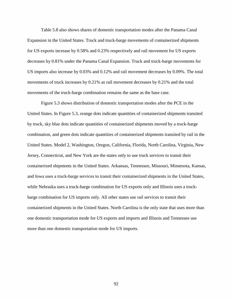
92
Table 5.8 also shows shares of domestic transportation modes after the Panama Canal
Expansion in the United States. Truck and truck-barge movements of containerized shipments
for US exports increase by 0.58% and 0.23% respectively and rail movement for US exports
decreases by 0.81% under the Panama Canal Expansion. Truck and truck-barge movements for
US imports also increase by 0.03% and 0.12% and rail movement decreases by 0.09%. The total
movements of truck increases by 0.21% as rail movement decreases by 0.21% and the total
movements of the truck-barge combination remains the same as the base case.
Figure 5.3 shows distribution of domestic transportation modes after the PCE in the
United States. In Figure 5.3, orange dots indicate quantities of containerized shipments transited
by truck, sky blue dots indicate quantities of containerized shipments moved by a truck-barge
combination, and green dots indicate quantities of containerized shipments transited by rail in the
United States. Model 2, Washington, Oregon, California, Florida, North Carolina, Virginia, New
Jersey, Connecticut, and New York are the states only to use truck services to transit their
containerized shipments in the United States. Arkansas, Tennessee, Missouri, Minnesota, Kansas,
and Iowa uses a truck-barge services to transit their containerized shipments in the United States,
while Nebraska uses a truck-barge combination for US exports only and Illinois uses a truck-
barge combination for US imports only. All other states use rail services to transit their
containerized shipments in the United States. North Carolina is the only state that uses more than
one domestic transportation mode for US exports and imports and Illinois and Tennessee use
more than one domestic transportation mode for US imports.

93
Figure 5.3. Distribution of domestic transportation modes after the Panama Canal Expansion in
the United States.
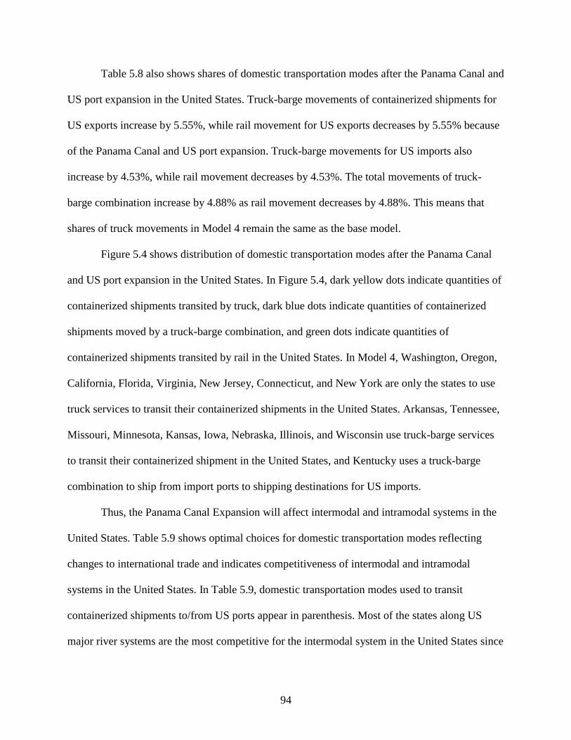
94
Table 5.8 also shows shares of domestic transportation modes after the Panama Canal and
US port expansion in the United States. Truck-barge movements of containerized shipments for
US exports increase by 5.55%, while rail movement for US exports decreases by 5.55% because
of the Panama Canal and US port expansion. Truck-barge movements for US imports also
increase by 4.53%, while rail movement decreases by 4.53%. The total movements of truck-
barge combination increase by 4.88% as rail movement decreases by 4.88%. This means that
shares of truck movements in Model 4 remain the same as the base model.
Figure 5.4 shows distribution of domestic transportation modes after the Panama Canal
and US port expansion in the United States. In Figure 5.4, dark yellow dots indicate quantities of
containerized shipments transited by truck, dark blue dots indicate quantities of containerized
shipments moved by a truck-barge combination, and green dots indicate quantities of
containerized shipments transited by rail in the United States. In Model 4, Washington, Oregon,
California, Florida, Virginia, New Jersey, Connecticut, and New York are only the states to use
truck services to transit their containerized shipments in the United States. Arkansas, Tennessee,
Missouri, Minnesota, Kansas, Iowa, Nebraska, Illinois, and Wisconsin use truck-barge services
to transit their containerized shipment in the United States, and Kentucky uses a truck-barge
combination to ship from import ports to shipping destinations for US imports.
Thus, the Panama Canal Expansion will affect intermodal and intramodal systems in the
United States. Table 5.9 shows optimal choices for domestic transportation modes reflecting
changes to international trade and indicates competitiveness of intermodal and intramodal
systems in the United States. In Table 5.9, domestic transportation modes used to transit
containerized shipments to/from US ports appear in parenthesis. Most of the states along US
major river systems are the most competitive for the intermodal system in the United States since
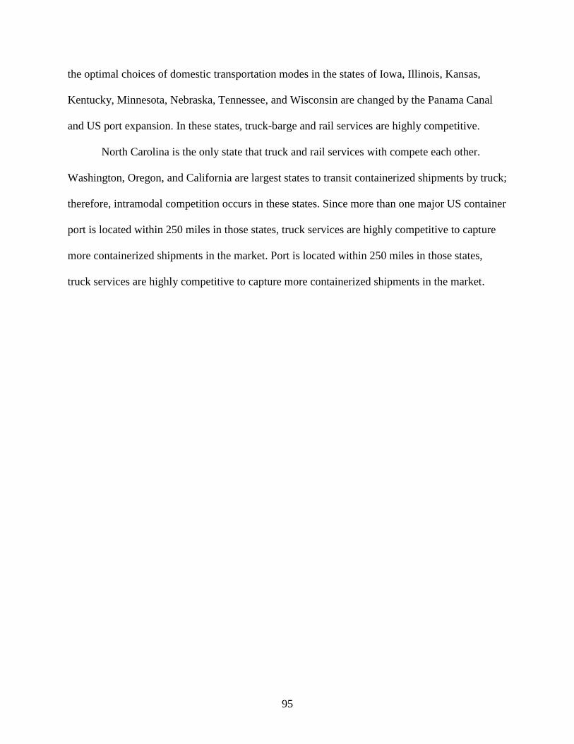
95
the optimal choices of domestic transportation modes in the states of Iowa, Illinois, Kansas,
Kentucky, Minnesota, Nebraska, Tennessee, and Wisconsin are changed by the Panama Canal
and US port expansion. In these states, truck-barge and rail services are highly competitive.
North Carolina is the only state that truck and rail services with compete each other.
Washington, Oregon, and California are largest states to transit containerized shipments by truck;
therefore, intramodal competition occurs in these states. Since more than one major US container
port is located within 250 miles in those states, truck services are highly competitive to capture
more containerized shipments in the market. Port is located within 250 miles in those states,
truck services are highly competitive to capture more containerized shipments in the market.

96
Figure 5.4. Distribution of domestic transportation modes after completion of the Panama Canal
and US port expansion in the United States.

97
Table 5.9. Optimal choices of US domestic transportation mode in changes of international trade
circumstance. US Export US Import
State Base
Model Model 2 Model 4 State
Base
Model Model 2 Model 4
CA LA/LB (T) LA/LB (T) LA/LB (T)
IA LA/LB (R) Gulf (T-B) Gulf (T-B) IA LA/LB (R) Gulf (T-B) Gulf (T-B)
IL Gulf (T-B)
M-A (R) M-A (R) Gulf (T-B) IL Gulf (T-B)
Gulf (T-B)
M-A (R) Gulf (T-B)
IN M-A (R) M-A (R) M-A (R)
KS LA/LB (R) Gulf (T-B) Gulf (T-B) KS LA/LB (R) Gulf (T-B) Gulf (T-B)
KY S-A (R) S-A (R) M-A (R) KY S-A (R) S-A (R) Gulf (T-B)
M-A (R)
LA S-A (R) S-A (R) S-A (R)
MN Gulf (T-B)
PNW (R) Gulf (T-B) Gulf (T-B)
MS S-A (R) S-A (R) S-A (R)
NC M-A (R) M-A (R)
S-A (T) M-A (R) NC
M-A (R)
S-A (R)
M-A (R)
S-A (T) M-A (R)
ND PNW (R) PNW (R) M-A (R) ND PNW (R) PNW (R) M-A (R)
NE LA/LB (R) Gulf (T-B) Gulf (T-B) NE LA/LB (R) LA/LB (R) Gulf (T-B)
OR PNW (T) PNW (T) PNW (T) OR PNW (T) PNW (T) PNW (T)
SD PNW (R) M-A (R) M-A (R) SD PNW (R) M-A (R) M-A (R)
TX LA/LB (R) LA/LB (R)
S-A (R) S-A (R) TX LA/LB (R) LA/LB (R)
LA/LB (R)
S-A (R)
WA PNW (T) PNW (T) PNW (T) TN Gulf (T-B) Gulf (T-B)
S-A (R) Gulf (T-B)
WI M-A (R) Gulf (T-B) M-A (R) WI M-A (R) M-A (R) Gulf (T-B)
Rail distance between shipping origin/destination in Indiana and export/import ports in
the South-Atlantic and Mid-Atlantic are almost the same as each other; therefore, rail services
are highly competitive in these areas. Louisiana and Mississippi are supposed to be competitive
for truck movements, because more than one major US container port is located within states or
interstate. However, these two states are highly competitive for rail services, since container
ports in or near these states meet their port capacities for other states’ shipments.
Containerized shipments in Arkansas and Missouri are always transited by a truck-barge
combination under the given scenarios because the distance between shipping

98
origins/destinations in those two states and export/import ports in the Gulf of Mexico could be
the optimal distance to minimize total domestic transportation costs. Then, those two states will
be able to use only a truck-barge combination. Lastly, since North and South Dakota are located
right in the Mid-North of the United States, long hauling of containerized shipments is required.
As a result, rail services are the only available choice for inland transportation mode in this study.
However, these two states become highly competitive for rail services when the Panama Canal
and US ports are expanded.
5.1.7. International Trade Volume and Flows of Containerized Shipments in the United
States
International trade flows of containerized shipments for US exports and import show
shipments between container ports in the United States and its trade partners in the world. Figure
5.5 shows ocean trade volume and flows of containerized shipments in the United States prior to
the Panama Canal Expansion. In Figure 5.5, a bar chart indicates quantities of containerized
shipments for US exports (green) and imports (red) on all possible ocean freight routes in the
United States. Ocean trades route in the United States are divided into 5 routes: (1) an ocean
trade route between US trade partners in Asia and the West Coast of the United States including
container ports in the PNW and LA.LB areas; (2) an ocean trade route between US trade partners
in Asia and the Gulf of Mexico including container ports in the West and East Gulf areas; (3) an
ocean trade route between US trade partners in Europe/South America and the Gulf of Mexico
including container ports in the West and East Gulf areas; (4) an ocean trade route between US
trade partners in Asia and the East Coast of the United States, including container ports in the
South Atlantic and Mid-Atlantic areas; and (5) an ocean trade route between US trade partners in
Europe/South America and the East Coast, including container ports in the South Atlantic and

99
Mid-Atlantic areas. One additional ocean trade route, named PNC in Figure 5.5 shows the total
volume of containerized shipments through the Panama Canal in the United States.
Figure 5.5. Ocean trade flows of containerized shipments in the United States.
Prior to the Panama Canal Expansion, more than 3.4 million TEUs of containerized
shipments are exported from the West Coast to importing counties in Asia, and 6.3 million TEUs
of containerized shipments are imported from exporting countries in Asia to the West Coast of
the United States. For shipments between the Gulf of Mexico and Asia through the Panama
Canal, more than 511,000 TEUs and 1.6 million TEUs of containerized shipments are transited
for US exports and imports, respectively. None of the containerized shipments are traded

100
between the Gulf of Mexico and US trade partners in Europe and South America in the base case.
Approximately 1.5 million TEUs of containerized shipments are exported from importing
countries in Asia to the East Coast of the United States through the Panama Canal and 2.9
million TEUs of containerized shipments are imported from exporting countries in Asia to the
East Coast of the United States via the Panama Canal. More than 1.9 million TEUs are exported
to importing countries in Europe and South America from the East Coast of the United States
and 3.5 million TEUs of containerized shipments are imported from exporting countries in
Europe and South America to the East Coast. 2 million TEUs and 4.5 million TEUs of
containerized shipment for US exports and import are shipped through the Panama Canal.
Figure 5.6 shows ocean trade volume and flows of containerized shipments by container
vessel in the United States after the Panama Canal Expansion. More than 3.1 million TEUs of
containerized shipments are exported from the West Coast to importing counties in Asia and 5.9
million TEUs of containerized shipments are imported from exporting countries in Asia to the
West Coast of the United States. For shipments between the Gulf of Mexico and Asia through
the Panama Canal, more than 78,000 TEUs and 350,000 TEUs of containerized shipments are
transited for US exports and import, respectively. 450 TEUs of containerized shipments are
exported to importing countries in Europe and South America from the Gulf of Mexico and
125,000 TEUs are imported from exporting countries in those two continents to the Gulf of
Mexico in the United States. More than 2.5 million TEUs of containerized shipments are
exported from importing countries in Asia to the East Coast through the Panama Canal and 4.6
million TEUs of containerized shipments are imported from exporting countries in Asia to the
East Coast via the Panama Canal. Approximately 1.2 million TEUs are exported to importing
countries in Europe and South America from the East Coast and 2.2 million TEUs of

101
containerized shipments are imported from exporting countries in Europe and South America to
the East Coast. More than 2.6 million TEUs and 4.9 million TEUs of containerized shipment for
US exports and import are transited through expanded Panama Canal.
Figure 5.6. Ocean trade flows of containerized shipments after the Panama Canal Expansion in
the United States.
Figure 5.7 shows ocean trade volume and flows of containerized shipments by container
vessel in the United States after the Panama Canal and US port expansion. More than 2.4 million
TEUs of containerized shipments are exported from the West Coast to importing counties in Asia
and 4.7 million TEUs of containerized shipments are imported from exporting countries in Asia
to the West Coast of the United States.
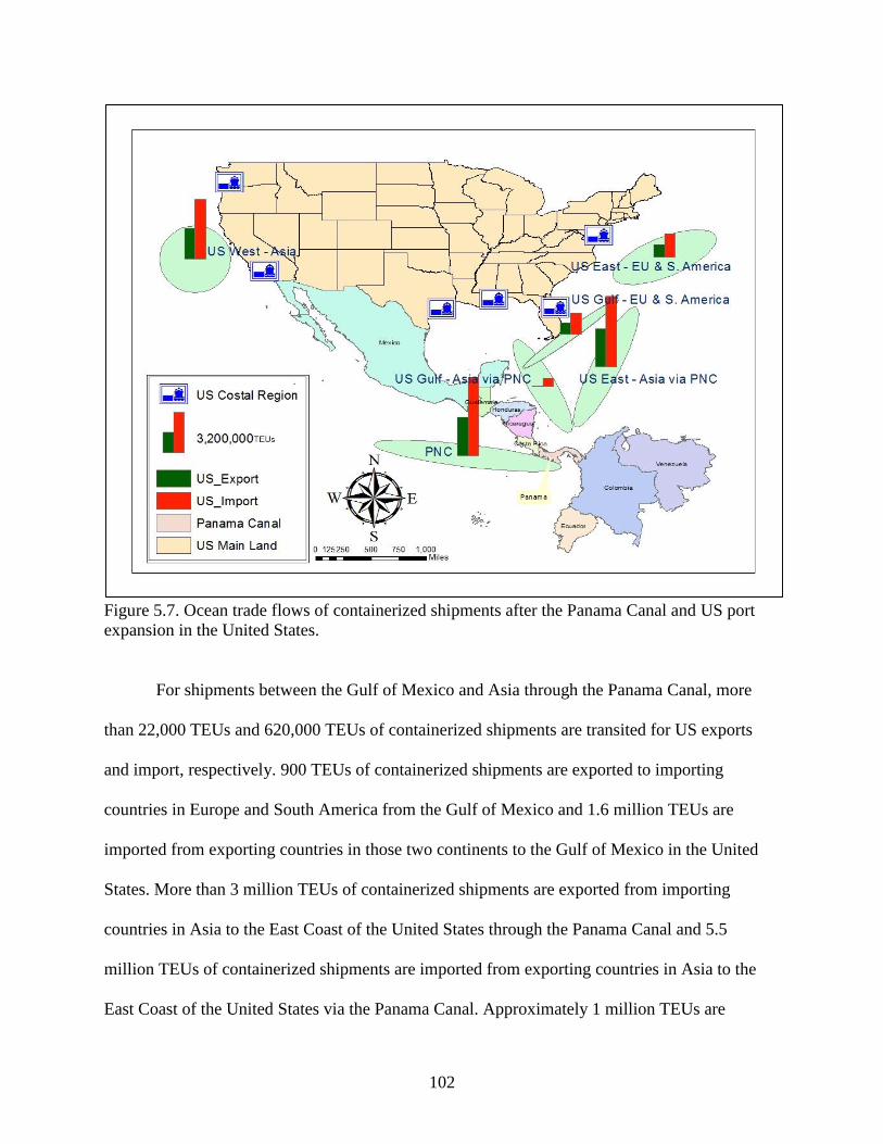
102
Figure 5.7. Ocean trade flows of containerized shipments after the Panama Canal and US port
expansion in the United States.
For shipments between the Gulf of Mexico and Asia through the Panama Canal, more
than 22,000 TEUs and 620,000 TEUs of containerized shipments are transited for US exports
and import, respectively. 900 TEUs of containerized shipments are exported to importing
countries in Europe and South America from the Gulf of Mexico and 1.6 million TEUs are
imported from exporting countries in those two continents to the Gulf of Mexico in the United
States. More than 3 million TEUs of containerized shipments are exported from importing
countries in Asia to the East Coast of the United States through the Panama Canal and 5.5
million TEUs of containerized shipments are imported from exporting countries in Asia to the
East Coast of the United States via the Panama Canal. Approximately 1 million TEUs are

103
exported to importing countries in Europe and South America from the East Coast of the United
States and 1.8 million TEUs of containerized shipments are imported from exporting countries in
Europe and South America to the East Coast of the United States. More than 3 million TEUs and
6.2 million TEUs of containerized shipment for US exports and import are transited through the
expanded Panama Canal.
As a result, Panama Canal Expansion affects international trade volume and flows of
containerized shipments between US and Asia. Table 5.10 shows shares and changes in
international trade volume of containerized shipments on selected routes in the United States.
Under current international trade conditions, 44.95% of the total containerized shipments in the
United States are traded between the West Coast of the United States and its trade partners in
Asia, 9.76% are on a route between the Gulf of Mexico in the United States and its trade partners
in Asia, 20.48% are on a route between East Coast of the United States and its trade partners in
Asia, and 24.81% of the total containerized shipments in the United States are traded between
the East Coast of the United States and its trade partners in Europe and South America. Shares of
international containerized shipments for US exports and imports at the Panama Canal is 30.24%,
since 27.21% of the total US export and 31.76% of the total US import are shipped through the
canal in the base case.
After the Panama Canal Expansion, quantities of the total containerized shipments
between the West Coast and Asia decrease to 41.57%, the total TEUs of containerized shipments
between the Gulf and Asia decrease to 1.96%, and the volume of the total containerized
shipments between the East Coast and EU/South America decreases to 15.79%. However, the
total quantities of containerized shipments between the Gulf and EU/S. America increase to 7.79%
and the total TEUs of containerized shipments between East Coast and Asia increase to 32.88%.
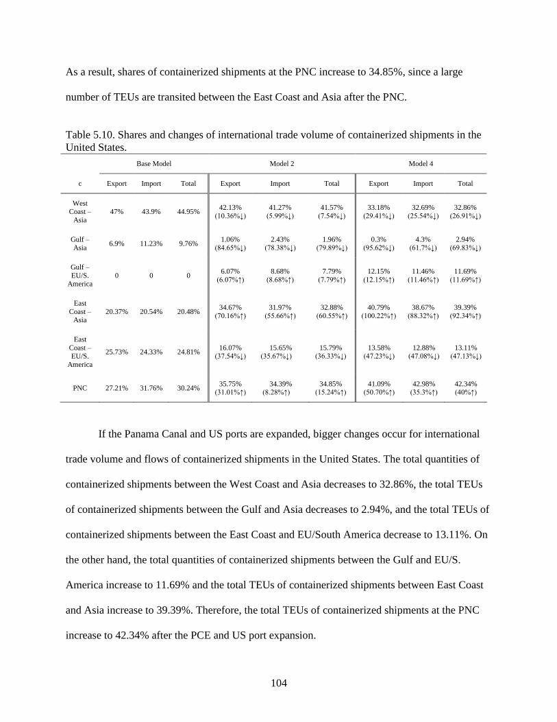
104
As a result, shares of containerized shipments at the PNC increase to 34.85%, since a large
number of TEUs are transited between the East Coast and Asia after the PNC.
Table 5.10. Shares and changes of international trade volume of containerized shipments in the
United States.
c
Base Model Model 2 Model 4
Export Import Total Export Import Total Export Import Total
West Coast –
Asia
47% 43.9% 44.95% 42.13%
(10.36%↓)
41.27%
(5.99%↓)
41.57%
(7.54%↓)
33.18%
(29.41%↓)
32.69%
(25.54%↓)
32.86%
(26.91%↓)
Gulf – Asia
6.9% 11.23% 9.76% 1.06%
(84.65%↓) 2.43%
(78.38%↓) 1.96%
(79.89%↓) 0.3%
(95.62%↓) 4.3%
(61.7%↓) 2.94%
(69.83%↓)
Gulf –
EU/S. America
0 0 0 6.07%
(6.07%↑)
8.68%
(8.68%↑)
7.79%
(7.79%↑)
12.15%
(12.15%↑)
11.46%
(11.46%↑)
11.69%
(11.69%↑)
East
Coast – Asia
20.37% 20.54% 20.48% 34.67%
(70.16%↑)
31.97%
(55.66%↑)
32.88%
(60.55%↑)
40.79%
(100.22%↑)
38.67%
(88.32%↑)
39.39%
(92.34%↑)
East
Coast – EU/S.
America
25.73% 24.33% 24.81% 16.07%
(37.54%↓) 15.65%
(35.67%↓) 15.79%
(36.33%↓) 13.58%
(47.23%↓) 12.88%
(47.08%↓) 13.11%
(47.13%↓)
PNC 27.21% 31.76% 30.24% 35.75%
(31.01%↑) 34.39%
(8.28%↑) 34.85%
(15.24%↑) 41.09%
(50.70%↑) 42.98%
(35.3%↑) 42.34% (40%↑)
If the Panama Canal and US ports are expanded, bigger changes occur for international
trade volume and flows of containerized shipments in the United States. The total quantities of
containerized shipments between the West Coast and Asia decreases to 32.86%, the total TEUs
of containerized shipments between the Gulf and Asia decreases to 2.94%, and the total TEUs of
containerized shipments between the East Coast and EU/South America decrease to 13.11%. On
the other hand, the total quantities of containerized shipments between the Gulf and EU/S.
America increase to 11.69% and the total TEUs of containerized shipments between East Coast
and Asia increase to 39.39%. Therefore, the total TEUs of containerized shipments at the PNC
increase to 42.34% after the PCE and US port expansion.
105
Thus, 45.29% of the total TEUs in the United States are shipped through the East Coast
and 44.95% of the total TEUs in the United States will be transited through the West Coast,
while 9.76% of the total TEUs in the United States will be handled at the Gulf. East and West
Coasts handle the majority of the containerized shipments in the United States evenly before the
PCE. The East Coast has an advantage with the completion of the new PCE, since it handles
48.67% of the total TEUs in the United States. Shares of the total containerized shipments in
West Coast will decrease from 44.95% to 41.75% after the PCE. However, the total quantities of
containerized shipments at the Gulf remain the same in the base case because all container ports
in the Gulf meet their capacities in all models. Therefore, although the total TEUs of
containerized shipments between the Gulf and Asia decreases as the total TEUs between the Gulf
and EU/South America increase, the total TEUs at the Gulf do not change before or after the
PCE. At the Gulf of Mexico, the ports’ capacities are relatively smaller than other container ports
in the United States; therefore, they have very limited capacities to handle containerized
shipments at ports under current trade conditions. If the Panama Canal and US ports are
expanded, the Gulf has an advantage with the PCE since it handles 14.63% of the total TEUs of
containerized shipments in the United States and the Gulf used to handle less than 10% of the
total TEUs. In the East Coast, container ports share 52.5% of the total containerized shipments in
the United States, while the West Coast loses their shipments dramatically. As a result, it is
concluded that the PCE brings positive effects for container ports in the East Coast and negative
effects on the ports in the West Coast, while no effects are felt by ports in the Gulf. The PCE and
US port expansion are significantly harmful to the ports in the West Coast, while they are the
most beneficial to the ports in the Gulf and the East Coast of the United States (Figure 5.8).

106
Figure 5.8. Total trade volume of containerized shipments by coastal regions in the United States.
5.1.8. Summary
The Panama Canal Expansion results in changes in international and domestic trade flows
because it allows larger container vessels transit through the canal. According to the result of the
ocean freight rate estimation, the ocean freight rate decreases as the vessel size increases. This
represents the lower ocean freight rates associated with economies of scale due to the increase in
vessel size for the hauling of containerized shipments. As a result, more containerized shipments
are transited through the expanded Panama Canal with a reduced ocean freight rate from using
larger vessel and eliminating delay by resolving congestion at the canal. However, the savings by
eliminating delays is relatively small compared with the reduction in the ocean freight rate.
9.8
9.1
7.2
2.1 2.1 3.2
9.9
10.6 11.5
6.6
7.6
9.2
0.0
2.0
4.0
6.0
8.0
10.0
12.0
14.0
Base Model Model 2 Model 4
West Coast Gulf of Mexico East Coast PNC
107
Therefore, the delay cost at the PNC does not affect trade volume and flows of containerized
shipments in the United States under the Panama Canal Expansion.
Since more than one inland transportation mode is available in states along US major
river systems, rail and barge-truck combinations are highly competitive in those states. Most
major US export and import states are located near the ocean and have cost advantages for
domestic transportation. In most coastal areas in the United States, more than one major
container port is located within a couple of hundred miles and this encourages competitiveness of
intermodal and intramodal systems. Since truck service has some advantages (cheaper cost and
better reliability, and accessibility for short hauling), truck service competes with rail service,
while it competes with other trucking services in the market. As a result, competitiveness of
intermodal and intramodal systems occurs at the same time in those states.
Because container ports in the Gulf of Mexico meet 100% of their capacities before and
after the PCE, trade volumes do not change. However, trade routes are changed significantly
after the PCE and US port expansion. States in the mid-north part of the US mainland have only
one choice for domestic transportation since distance between states and US sea ports are long.
Rail service is the most popular domestic transportation mode in those states; however, they have
choices of sea ports, depending on their international trade partners. Since those states could go
to all coastal regions in the United States with comparable costs for inland transportation, states
in the mid-north part of the US mainland are relatively more sensitive to inland transportation
costs than other states. Lastly, the PCE changes international trade volume and flows
dramatically. Most beneficial ports are located in the East Coast and the ports in the West Coast
have negative effects on their shipments.

108
Thus, most of states in the United States are sensitive to the PCE and US port expansion.
Competitiveness of intermodal and intramodal systems occurs in the United States. However, it
is not necessary to expand port capacities in the West Coast, while ports in the East Coast should
expand their capacities. Container ports in the Gulf should be or should not be expanded, under
various, alternative scenarios for this study.
5.2. Impacts of Changes in Toll Rates at the Panama Canal
This section introduces alternative toll rates at the Panama Canal to examine the impact
of changes in toll rates on trade flows of containerized shipments between the United States and
its top 15 trade partners. The model determines the optimal toll rate to maximize revenue at the
Panama Canal.
It is expected that the Panama Canal Authority (PCA) may increase or decrease toll rates
to maximize canal revenue. An increase (or a decrease) of the canal toll rates reduces (or
increases) the quantities of containerized shipments passing through the canal and also affects
inland shipping in the United States. The toll rate in the base case is $74 per TEU; alternatives
toll rates considered are decreases (and increases) of 5%, 10%, 15%, 20%, and 30%, respectively.
This section analyzes the increases and decreases in toll rates and examines the resulting
economic values of the Panama Canal Expansion.
5.2.1. Changes in Trade Volume of Containerized Shipments Transited through the
Panama Canal
Changes in toll rates at the PNC influence the total quantities of containerized shipments
at the canal. Table 5.11 shows changes in the total trade volume of containerized shipments
between the United States and its trading partners using alternative toll rates. Prior to the Panama
Canal Expansion, the US exports more than 2 million TEUs of containerized shipments to its

109
trade partners through the PNC, which is 27% of the total containerized shipments for US
exports. Approximately 4.5 million TEUs of containerized shipments are imported from other
countries to the US via the PNC, which is 32% of the total containerized shipments for US
imports. More than 6.6 million TEUs of the total containerized shipments are transited through
the PNC for US exports and imports. When the Panama Canal is expanded, the total TEUs of
containerized shipments for US exports through the PNC increase by 31% and, US imports
through the PNC increase by 8%, with the PNC toll rate remaining the same as in the base model.
The PNC handles more than 7.6 million TEUs of the total containerized shipments for US
exports and imports.
Table 5.11. Changes in trade volume of containerized shipments at the Panama Canal by the
PNC toll changes.
Toll Change
Toll at
the
PNC
($)
Trade Volume (TEUs) at the PNC Trade Volume (%) at the PNC
Export Import Total Export Import Total
Base
Mode
l
- $74 (-) 2,021,409 4,584,475 6,605,884 27% 32% 30%
Mode
l 2
- $74 (-) 2,648,310 4,964,146 7,612,456 36%
(31%↑)
34%
(8%↑) 34% (15%↑)
Decrease
$71.78
(3%↓) 2,861,928 5,272,567 8,134,495
39%
(8%↑)
37%
(6%↑) 37% (6.9%↑)
$70.3
(5%↓) 2,861,928 5,272,567 8,134,495
39%
(8%↑)
37%
(6%↑) 37% (6.9%↑)
$66.6
(10%↓) 2,861,928 5,272,567 8,134,495
39%
(8%↑)
37%
(6%↑) 37% (6.9%↑)
$62.9
(15%↓) 2,861,928 5,272,567 8,134,495
39%
(8%↑)
37%
(6%↑) 37% (6.9%↑)
$59.2
(20%↓) 2,861,928 5,272,567 8,134,495
39%
(8%↑)
37%
(6%↑) 37% (6.9%↑)
$51.8
(30%↓) 3,281,696 5,521,796 8,803,492
44%
(24%↑)
38%
(11%↑)
40%
(15.6%↑)
Increase
$77.4
(5%↑) 2,640,077 4,964,146 7,604,223
35%
( .3%↓) 34% (-) 35% (0.1%↓)
$81.4
(10%↑) 2,454,514 4,964,146 7,418,660
33%
(7%↓) 34% (-) 34% (2.5%↓)

110
Table 5.11. Changes in trade volume of containerized shipments at the Panama Canal by the
PNC toll changes (continued).
Toll Change
Toll at
the
PNC
($)
Trade Volume (TEUs) at the PNC Trade Volume (%) at the PNC
Export Import Total Export Import Total
$85.1
(15%↑) 2,454,514 4,964,146 7,418,660
33%
(7%↓) 34% (-) 34% (2.5%↓)
Mode
l 4
- $74 (-) 3,046,233 6,202,618 9,248,851 41%
(51%↑)
43%
(35%↑) 42% (40%↑)
Decrease
$70.3
(5%↓) 3,046,233 6,202,618 9,248,851
41%
(-) 43% (-) 42% (-)
$66.6
(10%↓) 3,046,233 6,352,964 9,399,197
41%
(-)
44%
(2.4↑) 43% (1.6%↑)
$62.9
(15%↓) 3,046,233 6,352,964 9,399,197
41%
(-)
44%
(2.4↑) 43% (1.6%↑)
$59.2
(20%↓) 3,046,233 6,352,964 9,399,197
41%
(-)
44%
(2.4↑) 43% (1.6%↑)
$51.8
(30%↓) 3,046,233 6,352,964 9,399,197
41%
(-)
44%
(2.4↑) 43% (1.6%↑)
Increase
$77.4
(5%↑) 3,046,233 6,202,618 9,248,851
41%
(-) 43% (-) 42% (-)
$81.4
(10%↑) 3,046,233 6,202,618 9,248,851
41%
(-) 43% (-) 42% (-)
$85.1
(15%↑) 3,046,233 6,202,618 9,248,851
41%
(-) 43% (-) 42% (-)
$88.8
(20%↑) 3,046,233 6,202,618 9,248,851
41%
(-) 43% (-) 42% (-)
$96.2
(30%↑) 3,046,233 6,202,618 9,248,851
41%
(-) 43% (-) 42% (-)
As an inverse relationship between the PNC toll rate and quantities of containerized
shipments through the PNC is expected, the quantity of containerized shipments through the
PNC increases when the PNC toll rate decreases. For instance, if 3% of the current toll rate at the
PNC decreases, TEUs of containerized shipments through the PNC increase by 6.9%. More than
8.1 million TEUs of containerized shipments are transited through the PNC when the toll is
reduced to $71.78 per TEU. However, if the PNC toll rates decrease by 10%, 15%, and 20%, the
total TEUs of containerized shipments through the PNC remains the same as that with the 3%
decrease. Trade balance of US exports and import through the PNC does not change as well.
However, if the PNC toll rate decreases from $74 to $51.8 (a 30% decrease), quantities of the

111
total containerized shipments through the PNC increase by 15.6%. The total quantities of
containerized shipments through the PNC for US exports and imports decrease by 0.1% with a 5%
decrease in the PNC toll rate. On the other hand, if the PNC toll rates increase by 10%, 15%,
20%, and 30%, the total number of containerized shipments through the PNC decrease from 7.6
million TEUs to 7.4 million TEUs. This implies that toll rates are not sensitive to the volume of
containerized shipments through the PNC.
If the Panama Canal and US ports are expanded, the total quantities of containerized
shipments through the PNC increase, as shown in Table 5.10. However, changes in the PNC rate
affect the total containerized shipments through the PNC only for US imports under some
instances of toll changes. The total TEUs of containerized shipments increase by 40%, with a 51%
increase for US exports and a 35% increase for US imports via the PNC after the PCE and US
port expansion. In quantity, more than 9.2 million TEUs of containerized shipments are transited
through the PNC after the PCE and US port expansion under the current toll rate. When the PNC
toll rate decreases by 5%, the quantities of US exports and imports remain the same as those in
the base case. However, if the PNC toll rates decrease by 10%, 15%, 20%, and 30%, quantities
of containerized shipments through the PNC for US imports increase by 1.6% from 6.2 million
TEUs to 6.3 million TEUs. Even if the PNC toll rates increase by 5%, 10%, 15%, 20%, and 30%,
the quantities of containerized shipments through the PNC in the United States do not change.
This implies that toll rates are not sensitive to the volume of containerized shipments through the
canal.
The PCE and US port expansion influence quantities of containerized shipments through
the Panama Canal significantly. In Model 2, four breaking points for the PNC toll rate are found
in regard to changes in the quantity of containerized shipments. The total quantities of

112
containerized shipments through the PNC increase with toll rate decreases in 3% and 30%, while
quantities of TEUs remain the same with toll rate decreases ranging between more than 3%
through 20%. The total quantities of containerized shipments through the PNC decrease with toll
rate increases in 5% and 10%, while quantities of TEUs remain the same with toll rate increases
ranging between more than 10% through 30%. On the other hand, in Model 4, only one breaking
point for the PNC toll rate is found in regard to changes in the quantity of containerized
shipments. The total quantity of containerized shipments through the PNC increases with a toll
rate decrease of 10%, while quantities of TEUs remain the same with toll rate decreases of more
than 10% through 30%. The total quantities of containerized shipments through the PNC do not
change with toll increases ranging between 5% through 30%.
5.2.2. Economic Value of the Panama Canal Expansion
The Panama Canal plays an important role in transporting shipments between the United
States and its trade partners in Asia. Without the canal, shipments between the Gulf of Mexico
and the East Coast of the United States and countries in Asia are transited through either the
Suez Canal, along the Atlantic Ocean or an alternative route along the Straits of Magellan. The
Panama Canal saves not only ocean transit time, but also the ocean transportation cost of
shipments passing between the Atlantic and Pacific Oceans. Since the Panama Canal has traffic
congestion due to increased shipments through the canal, the Panama Canal Authority (PCA)
decided to expand the canal.
Table 5.12 shows changes in the total toll revenue at the Panama Canal under alternative
PNC toll rates. Prior to the Panama Canal Expansion with a current toll rate as of $74 per TEU,
the total toll revenue is more than $488 million. When the PCE is completed, using the PNC toll
rate at the current level, the total toll revenue is more than $563 million, 15.2% higher than that
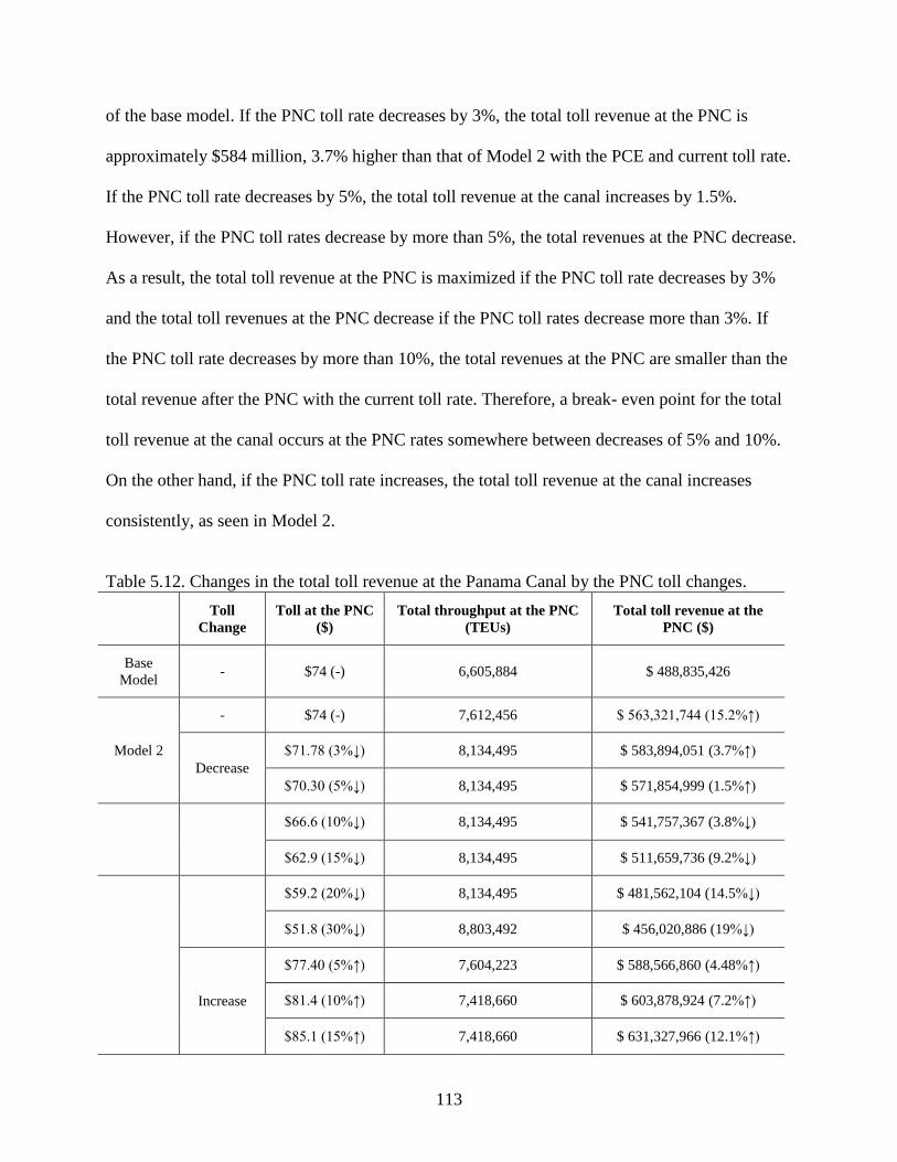
113
of the base model. If the PNC toll rate decreases by 3%, the total toll revenue at the PNC is
approximately $584 million, 3.7% higher than that of Model 2 with the PCE and current toll rate.
If the PNC toll rate decreases by 5%, the total toll revenue at the canal increases by 1.5%.
However, if the PNC toll rates decrease by more than 5%, the total revenues at the PNC decrease.
As a result, the total toll revenue at the PNC is maximized if the PNC toll rate decreases by 3%
and the total toll revenues at the PNC decrease if the PNC toll rates decrease more than 3%. If
the PNC toll rate decreases by more than 10%, the total revenues at the PNC are smaller than the
total revenue after the PNC with the current toll rate. Therefore, a break- even point for the total
toll revenue at the canal occurs at the PNC rates somewhere between decreases of 5% and 10%.
On the other hand, if the PNC toll rate increases, the total toll revenue at the canal increases
consistently, as seen in Model 2.
Table 5.12. Changes in the total toll revenue at the Panama Canal by the PNC toll changes.
Toll
Change
Toll at the PNC
($)
Total throughput at the PNC
(TEUs)
Total toll revenue at the
PNC ($)
Base
Model - $74 (-) 6,605,884 $ 488,835,426
Model 2
- $74 (-) 7,612,456 $ 563,321,744 (15.2%↑)
Decrease
$71.78 (3%↓) 8,134,495 $ 583,894,051 (3.7%↑)
$70.30 (5%↓) 8,134,495 $ 571,854,999 (1.5%↑)
$66.6 (10%↓) 8,134,495 $ 541,757,367 (3.8%↓)
$62.9 (15%↓) 8,134,495 $ 511,659,736 (9.2%↓)
$59.2 (20%↓) 8,134,495 $ 481,562,104 (14.5%↓)
$51.8 (30%↓) 8,803,492 $ 456,020,886 (19%↓)
Increase
$77.40 (5%↑) 7,604,223 $ 588,566,860 (4.48%↑)
$81.4 (10%↑) 7,418,660 $ 603,878,924 (7.2%↑)
$85.1 (15%↑) 7,418,660 $ 631,327,966 (12.1%↑)

114
Table 5.12. Changes in the total toll revenue at the Panama Canal by the PNC toll changes
(continued).
Toll
Change
Toll at the PNC
($)
Total throughput at the PNC
(TEUs)
Total toll revenue at the
PNC ($)
$88.8 (20%↑) 7,418,660 $ 658,777,008 (17%↑)
$96.2 (30%↑) 7,418,660 $ 713,675,092 (26.7%↑)
Model 4
- $74 (-) 9,248,851 $ 684,414,974 (40%↑)
Decrease
$70.3 (5%↓) 9,248,851 $ 650,194,225 (15.4%↑)
$66.6 (10%↓) 9,399,197 $ 625,986,520 (11.1%↑)
$62.9 (15%↓) 9,399,197 $ 591,209,491 (5%↑)
$59.2 (20%↓) 9,399,197 $ 556,432,462 (1.2%↓)
$51.8 (30%↓) 9,399,197 $ 486,878,405 (13.6%↓)
Increase
$77.4 (5%↑) 9,248,851 $ 715,861,067 (27.1%↑)
$81.4 (10%↑) 9,248,851 $ 752,856,471 (33.6%↑)
$85.1 (15%↑) 9,248,851 $ 787,077,220 (40%↑)
$88.8 (20%↑) 9,248,851 $ 821,297,969 (45.8%↑)
$96.2 (30%↑) 9,248,851 $ 889,739,466 (58%↑)
In Model 4, the total toll revenue at the PNC increases by 40%, mainly due to the Panama
Canal and US port expansion, while the toll rate at $74. Compare to Model 4, which includes the
PCE and US port expansion with the current toll rate, if the PCA decreases the toll rate at the
canal by 5%, 10%, and 15%, total revenues increase by 15.4%, 11.1%, and 5%, respectively
although changes in percentage are decreased. The total revenue decreases if the PNC toll rates
decrease by more than 20%. However, if the PNC toll rate increases, the total toll revenue at the
canal increases as well in Model 4.
Thus, if the Panama Canal Authority does not decrease the toll rate more than 5% or the
PCA increases the toll rate by any amount less than 30%, the total toll revenue increases

115
consistently after the Panama Canal Expansion. If the PCA decreases the toll rate less than 15%,
the total revenue at the canal also increases, while the total revenue increases consistently as the
toll rate increase at the canal after the Panama Canal and US port expansion. As a result,
although the PCE and US port expansion results in changes of the total toll revenue at the canal
associated with the total quantities of containerized shipments through the canal and the toll rate
at the canal, the total quantities of containerized shipments through the canal in the United States
are not sensitive to changes of the toll rate at the canal. In addition, the PNC toll changes would
account for a small portion of total ocean transportation costs and it will not affect the quantities
of shipments through the expanded canal significantly.
5.2.3. Summary
An optimal toll rate after the Panama Canal and US port expansion, to maximize the total
toll revenue at the PNC, is inconclusive. Theoretically, expansions would decrease the PNC toll
rate due to the economies of scale by use of larger container vessels after the PCE. However, an
optimal toll rate cannot be found in this study mainly because the toll rate is not sensitive to the
quantity of containers shipped through the canal. The toll rate at the PNC accounts for a small
portion of total transportation cost to transit containerized shipments between the United States
and its trading partners.
Figure 5.9 shows changes in the total volume (upper side) and toll revenue (lower side)
under alternative toll rates at the Panama Canal. In Figure 5.9, the blue line indicates volume of
containerized shipments with the current and alternative toll rates (Model 2) and the Panama
Canal Expansion. The red line indicates those under Model 4, which includes the Panama Canal
and US port expansion. Figure 5.9 also includes the total volume and revenue at the PNC for the
base model with current toll rate at $74*. The total volume of containerized shipments through

116
the Panama Canal either increases as the PNC toll rate decreases and the total volume decreases
as toll rate increases in Model 2. More specifically, the total quantities of containerized
shipments through the PNC does not change when the PNC toll rates change from 3% to 20%
decreases and from 10% to 30% increases. In Model 4, the total volume through the PNC
increases as the PNC toll decreases slightly and the total volume remains when the PNC toll rate
increases. The total volume of containerized shipments through the PNC remains the same with
the toll rate decreased from 10% to 30%.
The total toll revenue at the Panama Canal consistently increases as the PNC toll rate
increases in both Models 2 and 4 because the total volume at the canal either remains or slightly
decreases. The total revenue at the canal decreases as the toll rate decreases in Model 4. On the
other hand, the total revenue increases when the PNC toll rate decreases by less than 5% and the
total revenue begins to decrease somewhere between 5% and 10% decreases of the PNC toll rate
in Model 2. As a result, the Panama Canal Authority will earn more revenue from the toll unless
they decrease the toll rate by less than 5% of the current toll rate at the canal.
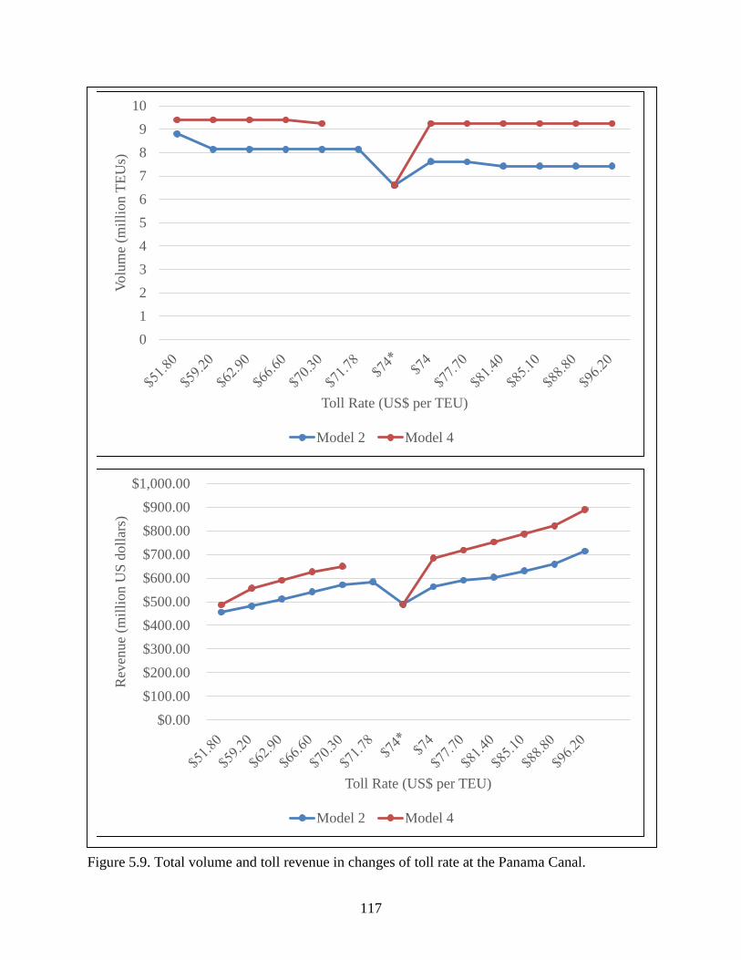
117
Figure 5.9. Total volume and toll revenue in changes of toll rate at the Panama Canal.
0
1
2
3
4
5
6
7
8
9
10V
olu
me
(mil
lion T
EU
s)
Toll Rate (US$ per TEU)
Model 2 Model 4
$0.00
$100.00
$200.00
$300.00
$400.00
$500.00
$600.00
$700.00
$800.00
$900.00
$1,000.00
Rev
enu
e (m
illi
on U
S d
oll
ars)
Toll Rate (US$ per TEU)
Model 2 Model 4

118
CHAPTER 6. SUMMARY AND CONCLUSIONS
The transportation of containerized shipments will continue to be a topic of interest in the
world because it is the major method used to ship various cargo globally. The reason for
continuous studies on the topic of transportation of containerized shipments is due mainly to a
significant increase in world container traffic since 1990. The majority of cargo is containerized
mainly due to advancement in the technology of container design. Since the United States is one
of the leaders in global trade, a large number of containerized shipments are exported and
imported in the United States.
In the United States, 80% of containerized shipments are imported from its top 15
exporting countries and 60% of containerized shipments are exported to its top 15 importing
countries. The majority of these countries are located in Northeast Asia and Europe, although
some trading partners are in other continents. Since the United States is a trade deficit country in
containerized shipments, most major container ports in the United States handle more import
shipments than export shipments. Furthermore, more than 95% of US cargo imports arrive on d
by ships (US Department of Transportation, 2009). Factors determining costs for shipping
containerized shipments between the US and its trading partners include domestic transportation
costs, ocean transportation costs, cargo handling charges at ports, and other costs (such as the toll
at the Panama Canal when vessel is required to navigate via the canal).
The Panama Canal is being expanded to reduce traffic congestions, stemming from the
increase in global trade between countries. The growth of world trade has led to the greater cargo
hauling of container vessels, and the increase in the number of these larger vessels being
manufactured. Fleets of a new class of Panamax ships continue to rise to satisfy a continuous
increase in containerized shipments under globalization.

119
The primary objective of this paper is to evaluate the impact of the Panama Canal
Expansion on the domestic and international trade flows of containerized shipments from
shipping origins in the US to ports in its importing countries for US exports and from the ports in
exporting countries to shipping destinations in the US for US imports. Special attention is given
to flows of containerized shipments between the US and its trade partners in Asia. More
specifically, the study is designed to undertake the following issues: (1) analyze the optimal trade
flows for US containerized shipments under the current shipping conditions, (2) estimate the
impact of the Panama Canal Expansion on the trade flows of US containerized shipments, (3)
estimate the impact of the Panama Canal and US port expansion on US containerized shipments,
(4) examine the effects of delay cost and toll rate at the Panama Canal for US containerized
shipments, and (5) evaluate the economic value of the Panama Canal Expansion.
Many studies have analyzed transportation of containerized shipments and its impacts on
trade flows among nations. The studies are, in general, focused on a spatial optimization of
containerized shipments. A spatial optimization model based on a linear programming algorithm
was developed to optimize trade flows by either minimizing costs or maximizing volumes. Most
of the previous studies were focused on US imports.
This study developed a spatial optimization model based on a mathematical programming
algorithm to examine the economic effects of the PCE on US trade with its trading partners,
especially those in Asia. The model minimizes total transportation costs associated with the
transportation of containerized shipments, in order to get them from their shipping origins to US
export ports and then also from export ports to the ports in importing countries for US exports
and from the ports in exporting countries to US import ports and then also from the import ports

120
to the shipping destinations in US for US imports. The objective function is minimized subject to
a system of linear constraints.
This study shows that there would be a significant change in the quantity of containerized
shipments transited through the canal and the toll revenue at the canal after its expansion. The
East Coast of the United States receives the most benefit under the Panama Canal Expansion
mainly because a decrease in ocean transportation costs from ports in the East Coast to Asia
leads to more domestic shipments to the East Coast from other ports in the US. Therefore, ports
in the East Coast of the United States would be beneficial if the ports expand their capacities to
handle increased shipments in the future. On the other hand, the ports in the West Coast would
lose quantities of containerized shipments after the Panama Canal Expansion because more
shipments would change domestic transportation routes from the West Coast to either the Gulf of
Mexico or the East Coast of the United States. This implies that the ports in the West Coast of
the United States would see a negative impact under the Panama Canal Expansion.
The Panama Canal Expansion will have no effect on US containerized shipments to ports
in the Gulf of Mexico because of two reasons: (1) ports in the Gulf Coast meet 100% of their
port capacities before and after the Panama Canal Expansion and (2) the majority of their
shipments are transited to/from ports in Asia through the PNC before the PCE, but many
shipments are transited to/from the ports in either Europe or South America after the PCE. In
other words, containerized shipments between the US Gulf Coast and either Europe or South
America fully replace lost quantities between the US Gulf Coast and Asia under the Panama
Canal Expansion. As a result, Gulf Coast ports may or may not need expansion of their port
capacities.

121
This study is inconclusive in determining the optimal toll rate at the canal which
maximizes its revenue. This may be mainly because the delay cost and toll rate at the canal
account for a small portion of the total transportation costs to transit containerized shipments
through the expanded canal. The sensitivity analysis indicates that changes in the toll rate
ranging between 5% and 30% are not sensitive to shipments via the canal, including that the
PNC should increase the toll rate to maximize its revenue under the assumption that US freight
rates, such as the rail rate, remain constant. Since shipping routes from shipping origins in most
states in the US to Asia through the West Coast competes with those through the PNC, changes
in domestic transportation costs (e.g., rail rate) to the West Coast may be an important factor
affecting containerized shipments via the Canal. Therefore, increases in the PNC toll rate to
maximize its revenue should be constrained by US shipments through the West Coast. This is
also true for containerized shipments for US imports from Asia.

122
REFERENCES
AECOM. (2012) NC Maritime Strategy Vessel Size vs. Cost. Report for the North Carolina
Department of Transportation.
Alabama State Port Authority. (2014) Port capacity and maximum vessel size.
http://www.asdd.com/index.html, accessed 17 July 2014.
ALK Technologies Inc. (2014) PC Miler Rail 19 BatchPro and PC Miler 24 BatchPro.
Behar, Alberto and Venables, J. (2010) Transportation costs and International Trade. From the
SelectedWorks of Alberto Behar,
http://works.bepress.com/cgi/viewcontent.cgi?article=1016&context=alberto_behar
Binkley, K. and Harrer, Bruce. (1981) Major Determinants of Ocean Freight Rates for Grains:
An Econometric Analysis. American Journal of Agricultural Economics 63(1):47-57.
Busan Port Authority. (2014) Port capacity and maximum vessel size.
http://www.busanpa.com/Service.do?id=engmain, accessed 16 July 2015.
Clarkson Research. (2014) Shipping Intelligence Network.
http://www.clarksons.net/sin2010/ts/Default.aspx?MyTs=1, accessed 9 September 2014.
Drewry Shipping Consultants Limited. (2015) Container Census 2013: Survey and Forecast of
Global Container Units.
Fan, L., Wilson, W., and Dahl, B. (2012) Congestion, port expansion and spatial competition for
US container imports. Transportation Research Part E 48(2012):1121-1136.
Fuller, Stephen, Makus, Larry, and Gallimore, William. (1984) Effects of Increasing Panama
Canal Toll Rates on U.S. Grain Exports. Southern Journal of Agricultural Economics. p.
9-20.
Georgia Ports Authority. (2014) Port capacity and maximum vessel size.
http://www.gaports.com/PortofSavannah.aspx, accessed 17 July 2014.
Hong Kong Container Terminal Operators Association Ltd. (2014) Port capacity and maximum
vessel size. http://www.hkctoa.com/, accessed 16 July 2014.
Hummels, David. (2007) Transportation Costs and International Trade in the Second Era of
Globalization. The journal of Economic Perspectives 21(3):131-154.
Jawaharlal Nehru Port Trust. (2014) Port capacity and maximum vessel size.
http://www.jnport.gov.in/index.aspx, accessed 16 July 2014.
Jakarta International Container Terminal. (2014) Port capacity and maximum vessel size.
https://www.jict.co.id/, accessed 16 July 2014.
Koo, W. and Kennedy, P. (2005) International Trade and Agriculture 1st Edition. Blackwell
Publishing Ltd.
Koo, W. and Thompson, S. (1982) An Economic Analysis of the U.S. Grain Marketing and
Transportation System. North Dakota State University Agricultural Experiment Station
Research Report 65(1):183-189.
123
Koenning, L. (2014) Personal interview regarding to the current status of container-on-barge
services in the United States. Account Manager and Operations at Osprey Line LLC.
interviewed 24 July 2014.
Korinek, Jane. and Sourdin, Patricia. (2010) Clarifying Trade Costs: Maritime Transport and Its
Effect on Agricultural Trade. Applied Economic Perspectives and Policy 32(3):417-435.
Limao, Nuno and Venables J. (2001) Infrastructure, Geographical Disadvantage, Transportation
Costs, and Trade. The World Bank Economic Review 15(3):451-479.
Marine Department, The Government of the Hong Kong Special Administrative Region. (2014)
Port capacity and maximum vessel size. http://www.mardep.gov.hk/en/home.html,
accessed 16 July 2015.
Mitsui O.S.K. Lines. (2014) Landside Tariff Surcharge. http://cms.molpower.com/Tariffs-
/Surcharge-Website, accessed 9 October 2014.
Leam Chabang International Terminal Co., Ltd. (2014) Port capacity and maximum vessel size.
http://www.lcit.com/, accessed 16 July 2014.
Orient Overseas Container Line, Ltd (OOCL). (2014) Local and Haulage Surcharges.
http://www.oocl.com/eng/resourcecenter/globalinfo/Pages/default.aspx, accessed 20
October 2014.
Panama Canal Authority. (2006) Annual Report. http://www.acp.gob.pa/eng/general/reporte-
anual/annual-report-2006.pdf, accessed 20 January 2014.
Panama Canal Authority. (2010) Annual Report. http://www.acp.gob.pa/eng/general/reporte-
anual/2010/pdf/LIBROing.pdf, accessed 12 November 2013.
Panama Canal Authority. (2012) Annual Report. http://www.acp.gob.pa/eng/general/reporte-
anual/2012/pdf/ingles.pdf, accessed 6 May 2013.
Panama Canal Authority. (2013) Annual Report. http://www.pancanal.com/eng/general/reporte-
anual/2013/pdf/Report-v2.pdf, accessed 17 December 2014.
Panama Canal Authority. (2014) Annual Report. http://www.pancanal.com/eng/general/reporte-
anual/2014/FlipBook.html, accessed 23 February 2015.
Panama Canal Authority. (2015) Proposal to Modify the Regulations for the Admeasurement of
Vessels and the Panama Canal Tolls System. http://www.pancanal.com/peajes/pdf/tolls-
proposal-2015.pdf, accessed 9 March 2015.
Pagano, A., Light, M., Sánchez, O., Ungo, R., and Tapiero, E. (2012) Impact of the Panama
Canal expansion on the Panamanian economy. Maritime Policy & Management: The
flagship journal of international shipping and port research 39(7):705-722.
Pagano, A., Wang, G., Sánchez, O., and Ungo, R. (2013) Impact of privatization on port
efficiency and effectiveness: results from Panama and US ports. Maritime Policy &
Management: The flagship journal of international shipping and port research 40(2):100-
115.
Park, J. and Koo, W. (2004) An Economic Analysis of Ocean Freight Rates for Grain Shipments
from the United States to Major Importing Countries. Journal of the Transportation
Research Forum. Vol.43:85-100.

124
Port Freeport. (2014) Port capacity and maximum vessel size. http://www.portfreeport.com/,
accessed 17 July 2014.
Port Miami. (2014) Port capacity and maximum vessel size.
http://www.southfloridacontainer.com/, accessed 17 July 2014.
Port of Antwerp. (2014) Port capacity and maximum vessel size.
http://www.portofantwerp.com/en, accessed 16 July 2014.
Port of Bremerhaven/Bremen. (2014) Port capacity and maximum vessel size.
http://www.bremenports.de/en/location, accessed 16 July 2014.
Port of Felixstowe. (2014) Port capacity and maximum vessel size.
https://www.portoffelixstowe.co.uk/, accessed 16 July 2014.
Port of Gulfport. (2014) Port capacity and maximum vessel size.
http://shipmspa.com/#sthash.WFjKfjI4.dpbs, accessed 17 July 2014.
Port of Hamburg. (2014) Port capacity and maximum vessel size.
http://www.portofhamburg.com/en, accessed 16 July 2014.
Port of Houston Authority. (2014) Port capacity and maximum vessel size.
http://www.portofhouston.com/, accessed 17 July 2014.
Port of Kaohsiung, Taiwan International Ports Corporation, Ltd. (2014) Port capacity and
maximum vessel size. http://kh.twport.com.tw/en/, accessed 16 July 2014.
Port of Long Beach. (2014) Port capacity and maximum vessel size. http://www.polb.com/,
accessed 17 July 2014.
Port of New Orleans. (2014) Port capacity and maximum vessel size. http://www.portno.com/,
accessed 17 July 2014.
Port of New York and New Jersey. (2014) Port capacity and maximum vessel size.
http://www.panynj.gov/port/, accessed 17 July 2014.
Port of Portland. (2014) Port capacity and maximum vessel size.
http://www2.portofportland.com/Marine, accessed 17 July 2014.
Port of Rotterdam. (2014) Port capacity and maximum vessel size.
http://www.portofrotterdam.com/en/Pages/default.aspx, accessed 16 July 204.
Port of Seattle. (2014) Port capacity and maximum vessel size.
http://www.portseattle.org/Cargo/SeaCargo/Facilities/Container-
Terminals/Pages/default.aspx, accessed 17 July 2014.
Port of Tacoma, (2014) Port capacity and maximum vessel size. http://portoftacoma.com/,
accessed 17 July 2014.
Port of Yokohama. (2014) Port capacity and maximum vessel size.
http://www.city.yokohama.lg.jp/kowan/english/, accessed 16 July 2014.
Rodrigue, J., Comtois, C., and Slack, B. (2013) The Geography of Transport Systems. Third
Edition.
Santos Brasil. (2014) Port capacity and maximum vessel size.
https://www.santosbrasil.com.br/en-us/services/port-operations, accessed 16 July 2014.
125
Sea-distance. (2013) Ocean Distance Calculator. http://www.sea-distances.org/, accessed 8
August 2014.
Shanghai International Port (Group) Co., Ltd. (2014) Port capacity and maximum vessel size.
http://www.portshanghai.com.cn/en/, accessed 16 July 2014.
Shenzhen Port. (2014) Port capacity and maximum vessel size.
http://www.szport.net/eng/index.jsp, accessed 16 July 2014.
South Carolina Ports. (2014) Port capacity and maximum vessel size.
http://www.scspa.com/Cargo/Facilities/charleston/terminals/terminals.asp, accessed 17
July 2014.
The Port of Los Angeles. (2014) Port capacity and maximum vessel size.
http://www.portoflosangeles.org/, accessed 17 July 2014.
The Port of Virginia. (2014) Port capacity and maximum vessel size.
http://www.portofvirginia.com/facilities/norfolk-international-terminals-nit/, accessed 17
July 2014.
Tokyo Port Terminal Corporation. (2014) Port capacity and maximum vessel size.
http://www.tptc.co.jp/tabid/798/Default.aspx, accessed 16 July 2014.
Ungo, R. and Sabonge, R. (2012) A competitive analysis of Panama Canal routes. Maritime
Policy & Management: The flagship journal of international shipping and port research
39(6):555-570.
United Nations Conference on Trade and Development. (2013) Review of Maritime Transport
2013. http://unctad.org/en/publicationslibrary/rmt2013_en.pdf, accessed 16 March 2014.
US Bureau of Labor Statistics (2014) Local Area Unemployment Statistics (LAUS).
US Census Bureau (2014) Population Estimates: NST-EST2014-01.
US Department of Commerce. (2014) National Economic Account: Gross Domestic Product,
http://www.bea.gov/newsreleases/national/gdp/2014/pdf/gdp1q14_adv.pdf, accessed 1
May 2014.
US Department of Commerce. (2014) National Economic Account: 2013 NAICS Total All
Merchandise Exports and Imports.
US Department of Transportation. (2009) American Container Ports: Freight Hubs That Connect
Our Nation to Global Markets.
US Department of Transportation. (2014) Table 3-21: Average Freight Revenue Per Ton-Mile.
US Energy Information Administration. (2014) U.S. On-Highway Diesel Fuel Price.
US Maritime Administration. (2013)
http://www.marad.dot.gov/library_landing_page/data_and_statistics/Data_and_Statistics.
htm, accessed 20 November 2013.
US Maritime Administration. (2013) Panama Canal Expansion Study Phase I Report:
Developments in Trade and National and Global Economies.
http://www.marad.dot.gov/documents/Panama_Canal_Phase_I_Report_-_20Nov2013.pdf,
accessed 22 January 2014.

126
US Maritime Administration. (2013) 2008-2013 U.S. Container Trade by Trading Partners
Report.
US Surface Transportation Board. (2010) Study of Railroad Rates: STB Rail Rate Index 1985 to
2007.
US Surface Transportation Board. (2010) Economic data: Waybill.
http://www.stb.dot.gov/stb/industry/econ_waybill.html, accessed 16 February 2014.
Vietnam International Container Terminals. (2014) Port capacity and maximum vessel size.
http://www.vict-vn.com/Home.aspx, accessed 16 July 2014.
Wilson, W., Koo, W., Taylor, D., and Dahl, L. (2005) Fundamental Factors Affecting World
Grain Trade in the Next Two Decades. North Dakota State University Agribusiness &
Applied Economics Report No.555
Wilson, W., Koo, W., Taylor, D., and Dahl, L. (2005) Long-Term Forecasting of World Grain
Trade and U.S. Gulf Exports. Journal of Transportation Research Board. Vol.1909:22-30.
World Trade Organization. (2013) World Trade Report 2013: Factors shaping the future of world
trade. http://www.wto.org/english/res_e/booksp_e/world_trade_report13_e.pdf, accessed
1 March 2014.
World Shipping Council. (2014) Trade Statistics. http://www.worldshipping.org/about-the-
industry/global-trade, accessed 14 December 2014.

127
APPENDIX A. EXPORT DEMAND AND IMPORT SUPPLY FOR US EXPORTS (TEUs)

128
Table A1. Export Demand and Import Supply for US Exports (TEUs)
Shipping
Origin
Importing Countries
Supply Belgiu
m Brazil China
German
y
Hong
Kong India
Indones
ia Italy Japan
Netherl
ands
South
Korea Taiwan
Thailan
d
United
Kingdom
Viet
Nam
Alabama 2567 4570 59741 12491 2196 3466 970 1579 9400 1193 8096 4447 2144 2762 1610 117233
Arkansas 1597 1573 15103 840 2063 737 1185 487 2618 265 2889 2159 521 681 937 33655
Arizona 987 2579 27742 4047 4101 1320 1009 1562 11124 1841 4525 7938 6468 3504 1891 80639
California 28830 19058 369930 29366 80707 63577 22820 16042 165401 23569 131642 160211 24010 18248 44136 1197546
Colorado 1454 1096 16395 1547 2281 1812 1315 563 5365 1570 4376 4045 1100 923 1584 45428
Connecticut 3559 2416 24171 7889 2167 2222 1285 1169 7163 2703 8455 2802 1130 2795 1247 71173
District of
Columbia
14 81 111 56 12 320 11 286 46 4 22 62 3 140 9 1175
Delaware 4200 760 11055 1494 382 554 331 160 4014 1150 1908 2476 191 3031 386 32093
Florida 4371 36652 31975 8087 10804 14006 3604 3992 13217 5171 8164 7518 2826 4765 4064 159217
Georgia 7015 7706 88104 6048 8045 8079 7578 4357 16977 3537 13360 14966 2964 5060 11151 204946
Iowa 888 4168 16106 3574 1298 1296 1923 830 12059 1313 5017 2508 646 1448 1741 54816
Idaho 90 391 11124 183 3240 285 1389 162 3706 346 9331 16408 338 367 777 48138
Illinois 16935 17439 114210 14660 7116 15560 13529 3789 25858 6741 14067 24423 5134 8344 12266 300070
Indiana 4805 6427 31834 11170 4172 4063 1716 5652 20622 4626 12066 5621 1686 4640 1561 120662
Kansas 1061 3526 29185 2014 1324 1183 1886 1014 9733 449 3796 3664 599 1979 3206 64620
Kentucky 5017 8072 27557 4385 6598 1958 1330 1447 15409 3279 8228 6829 1540 6758 971 99378
Louisiana 11382 15575 204102 5876 663 9582 14618 3903 44467 16094 24193 11139 5185 4503 4549 375832
Massachusetts 7113 3066 49413 10510 11161 4772 1190 4209 24659 6054 15567 21528 2586 10138 1814 173781
Maryland 3499 2261 14873 1540 1402 3867 1762 1707 5761 2003 5618 2684 1064 2057 953 51051
Maine 569 171 6197 310 263 241 205 335 1513 358 1398 423 99 274 100 12455
Michigan 7356 5284 83941 10054 2421 3603 2130 3663 17473 1775 15826 4501 3711 2984 1106 165830
Minnesota 6585 2448 49444 4115 4580 3088 2642 2073 15136 2364 10694 11043 3755 2224 3117 123306
Missouri 4529 2159 26215 1816 1381 2144 2909 1511 7878 1517 9320 2417 1340 1363 1262 67762
Mississippi 3555 2955 16920 1001 900 1203 725 462 2454 1680 2047 1204 575 788 1148 37618
Montana 596 30 2648 198 42 358 95 107 670 110 2984 1708 45 103 138 9833

129
Table A1. Export Demand and Import Supply for US Exports (TEUs) (continued).
Shipping
Origin
Importing Countries
Supply Belgiu
m Brazil China
German
y
Hong
Kong India
Indones
ia Italy Japan
Netherl
ands
South
Korea Taiwan
Thailan
d
United
Kingdom
Viet
Nam
North Carolina 6801 5333 65405 5844 8117 5283 5728 1901 21581 3549 10062 7128 2058 3927 6319 159037
North Dakota 792 222 535 292 27 490 184 159 412 31 272 155 45 135 115 3867
Nebraska 987 637 12112 790 1826 341 846 910 6687 1001 4978 2344 631 258 2392 36741
New Hampshire
231 480 7300 1236 1619 474 170 604 1399 863 1393 1062 460 681 281 18253
New Jersey 10348 8477 40452 7611 8663 7928 3645 5064 20238 10700 18701 13578 2384 9118 2786 169692
New Mexico 238 226 2188 404 222 257 440 123 649 104 340 245 326 235 136 6133
Nevada 1078 408 13126 698 1819 16850 392 427 3117 367 1798 1045 433 586 305 42447
New York 28042 7084 114587 13154 91165 37598 3913 7704 29173 9034 25050 23984 10195 25151 4676 430510
Ohio 4931 11267 74469 7690 4487 7904 5766 3887 19426 3994 13979 9842 4274 6341 3082 181338
Oklahoma 851 1303 9390 1210 615 1145 1254 320 5003 646 1399 744 797 548 501 25726
Oregon 1100 2840 76674 2433 3915 2291 5271 994 20216 1142 16607 18267 2053 1322 17771 172897
Pennsylvania 9963 9306 77834 9833 4720 8326 4190 5156 21773 8771 16594 12320 2180 6470 2114 199551
Rhode Island 289 103 2195 1168 354 209 58 783 588 126 473 1611 324 295 216 8793
South Carolina 4427 4684 92529 20203 2849 7229 2160 2037 8443 2115 7838 6377 1809 5749 3393 171842
South Dakota 367 129 1637 134 181 29 127 71 641 20 280 165 81 75 134 4072
Tennessee 11897 5054 53205 4229 3622 4089 5121 2838 23216 4965 10176 7681 2475 3725 5363 147655
Texas 43466 73267 266972 15462 16484 33030 25297 9858 60415 48736 121499 89184 17294 16877 22870 860711
Utah 2099 750 21151 1490 46453 10018 1055 1291 6803 948 4217 13606 8900 19561 678 139019
Virginia 4086 4919 46860 4767 2397 4266 6597 1955 6553 2373 5309 10500 1424 4419 4465 110890
Vermont 244 44 15486 312 2990 181 208 161 1899 205 2317 3703 705 221 211 28887
Washington 4035 7973 350174 9967 24053 21537 48490 1977 95803 5407 49177 37272 10544 8813 9459 684682
Wisconsin 3855 3669 38161 4258 2923 5577 2086 2353 10758 1988 6601 4695 2687 2674 2358 94642
West Virginia 3052 4482 15973 1700 774 8839 294 4912 6519 4041 6305 1055 363 1909 363 60581
Wyoming 87 837 241 13 13 62 2169 3 633 221 679 953 442 93 383 6828
Demand 271840 303954 2726751 258174 389609 333248 213618 116547 814673 201060 649634 590242 142542 209061 192100

130
APPENDIX B. EXPORT DEMAND AND IMPORT SUPPLY FOR US IMPORTS (TEUs)

131
Table B1. Export Demand and Import Supply for US Imports (TEUs)
Shipping
Destination
Exporting Countries
Demand Belgium
Brazil China German
y Hong Kong
India Indones
ia Italy Japan
Netherlands
South Korea
Taiwan Thailan
d United
Kingdom Viet Nam
Alabama 1166 15898 40452 14102 837 986 1458 3476 5437 976 44770 1827 644 640 3831 136500
Arkansas 335 242 43350 1780 844 2518 521 905 610 555 1482 1644 1045 299 1004 57135
Arizona 382 943 52661 3086 7463 1784 1233 1794 6617 2992 3366 6748 3188 1548 1626 95432
California 7788 24696 2604119 60280 86888 34120 79124 28665 183998 12314 148000 148506 114294 12127 154326 3699245
Colorado 669 531 39427 3024 3442 4307 530 2683 945 1536 3055 2793 1043 903 4052 68940
Connecticut 2808 2995 56027 7894 3641 2302 1574 5116 4529 13820 1947 3705 1380 6482 3773 117991
District of
Columbia 43 78 396 235 61 177 9 241 161 367 136 13 30 131 37 2115
Delaware 14977 2524 10481 1589 435 1271 129 823 473 3197 178 415 46 9042 195 45775
Florida 4713 31140 237016 10287 20842 9670 8852 15265 18195 12087 14987 13716 10028 7279 27180 441257
Georgia 6208 7162 331080 61604 16111 15578 13267 13115 20444 8045 68015 13639 16616 6925 20686 618495
Iowa 465 1160 26230 3173 531 1682 224 3040 1768 737 1552 2439 557 370 1034 44962
Idaho 28 77 15925 388 548 119 278 3216 1979 348 4285 9167 71 77 574 37081
Illinois 8770 6823 526970 25575 11878 13167 11264 15860 38875 33159 63928 29327 13780 6844 21873 828092
Indiana 2170 4214 126175 11163 2746 4352 3093 6540 23039 4356 3744 11361 7320 4092 8456 222822
Kansas 1396 1532 44095 3955 1983 866 2201 2584 1112 781 2591 16580 794 1567 7136 89173
Kentucky 4458 2667 132175 9294 6769 8587 7670 14587 20858 2620 8161 19947 7598 3665 11009 260064
Louisiana 17276 18129 21214 3223 1097 4447 8984 2340 1490 5224 6888 1104 1675 2932 2584 98608
Massachusetts 2746 1636 98926 9067 6469 3165 4776 6460 4097 7401 4236 7975 4850 8161 6983 176948
Maryland 3103 7796 60704 25864 2352 5695 6638 6496 5638 2619 1936 2164 10243 4035 6256 151541
Maine 173 60 7368 2433 285 240 92 346 227 697 235 290 692 416 1198 14753
Michigan 2280 6190 137812 19867 3554 10318 3140 9182 18726 2335 23256 8785 8714 2453 3014 259628
Minnesota 1018 2601 205753 4783 2980 2265 1016 3938 2280 1475 2130 8033 2343 1300 2705 244621
Missouri 4629 1185 83320 5744 2071 3716 995 2471 1598 1320 2838 4601 1423 1336 2709 119956
Mississippi 179 10984 65871 2775 1014 2674 301 970 3297 1791 1250 2963 1137 3269 3338 101813
Montana 41 29 2138 742 46 79 5 93 36 36 177 168 25 68 18 3701

132
Table B1. Export Demand and Import Supply for US Imports (TEUs) (continued).
Shipping
Destination
Exporting Countries
Demand Belgium
Brazil China German
y Hong Kong
India Indones
ia Italy Japan
Netherlands
South Korea
Taiwan Thailan
d United
Kingdom Viet Nam
North Carolina 3691 8655 207937 16930 4679 12559 12235 13673 13293 5685 9103 10722 6727 7714 18384 351987
North Dakota 58 116 2907 706 16 700 59 375 357 54 523 179 174 112 562 6898
Nebraska 900 272 17947 1679 505 365 112 1253 1169 132 344 810 649 175 986 27299
New
Hampshire 159 158 18512 2374 708 1370 748 1069 423 1462 533 2297 998 673 1020 32504
New Jersey 33721 9017 346173 37686 14925 57592 20981 52518 42894 21701 31507 20565 14185 23797 23833 751093
New Mexico 261 36 15899 546 189 174 39 140 474 1627 159 479 533 267 67 20890
Nevada 648 940 59571 711 1900 1013 993 682 413 340 14863 4191 1378 460 1314 89418
New York 67117 12426 460945 19333 190866 104875 20513 50558 13459 10161 20194 31277 17461 15531 36940 1071657
Ohio 3739 5872 243296 23400 4637 10915 11421 9942 26445 4169 13015 14987 7942 3529 27961 411269
Oklahoma 1582 340 45714 1777 1697 1821 1429 1061 2081 347 823 2813 1328 680 1629 65122
Oregon 268 726 58654 3009 2106 1606 3019 1123 16530 1918 16289 4431 3121 419 7477 120697
Pennsylvania 22006 9598 346053 25147 6136 11873 6679 14399 9271 8641 32592 11495 4992 9372 16054 534309
Rhode Island 1130 655 25101 16676 584 1467 209 819 633 3049 358 748 1320 2170 429 55348
South Carolina 5738 6267 111239 34886 1722 8713 14398 10882 7921 7435 4595 4846 6770 4445 10208 240064
South Dakota 33 1055 2581 137 68 47 9 218 71 48 103 252 107 30 97 4857
Tennessee 11893 4082 435571 13076 4578 14862 17810 7598 39750 2961 5375 10632 9604 4477 28981 611252
Texas 19538 57407 825238 35917 18671 51829 17627 30721 32085 23693 99929 43821 38308 16894 42944 1354621
Utah 143 837 34627 945 2106 671 427 791 632 279 689 3768 362 269 1183 47728
Virginia 2611 5053 90504 9065 2281 9405 9528 7000 8726 2324 2138 3333 2730 3228 10185 168112
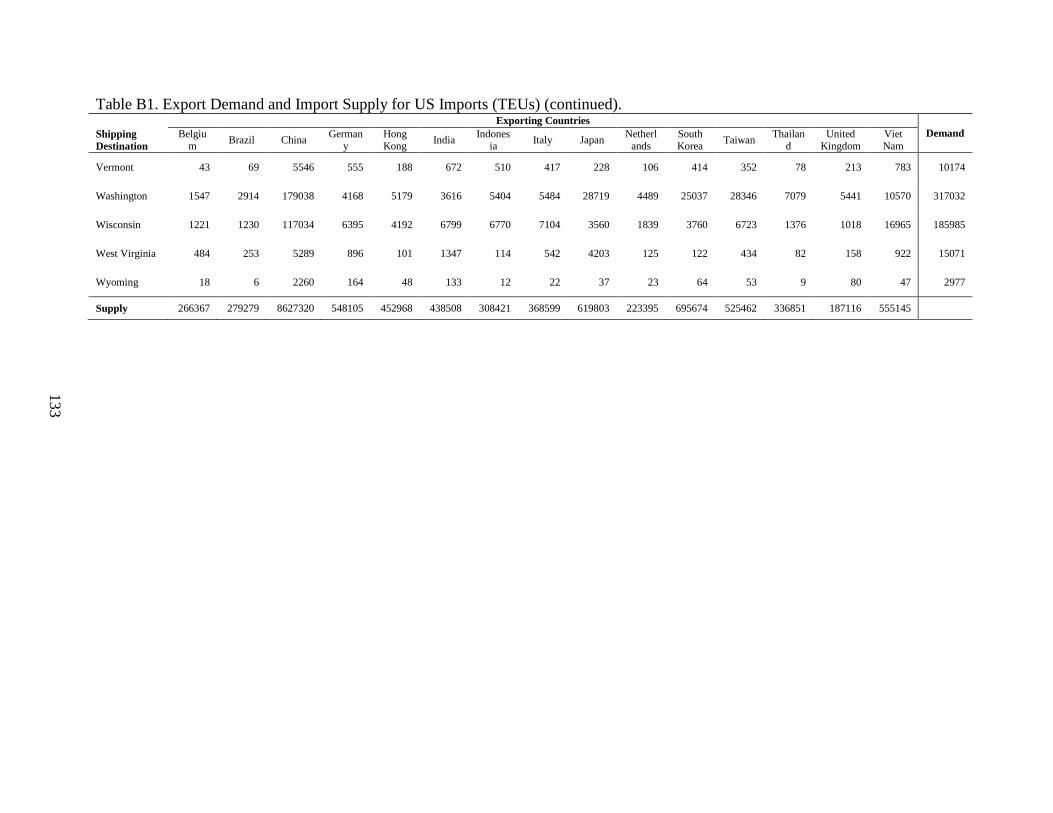
133
Table B1. Export Demand and Import Supply for US Imports (TEUs) (continued).
Shipping
Destination
Exporting Countries
Demand Belgium
Brazil China German
y Hong Kong
India Indones
ia Italy Japan
Netherlands
South Korea
Taiwan Thailan
d United
Kingdom Viet Nam
Vermont 43 69 5546 555 188 672 510 417 228 106 414 352 78 213 783 10174
Washington 1547 2914 179038 4168 5179 3616 5404 5484 28719 4489 25037 28346 7079 5441 10570 317032
Wisconsin 1221 1230 117034 6395 4192 6799 6770 7104 3560 1839 3760 6723 1376 1018 16965 185985
West Virginia 484 253 5289 896 101 1347 114 542 4203 125 122 434 82 158 922 15071
Wyoming 18 6 2260 164 48 133 12 22 37 23 64 53 9 80 47 2977
Supply 266367 279279 8627320 548105 452968 438508 308421 368599 619803 223395 695674 525462 336851 187116 555145

134
APPENDIX C. CARGO HANDLING COSTS (US$) AT PORTS IN EXPORTING AND
IMPORTING COUNTRIES
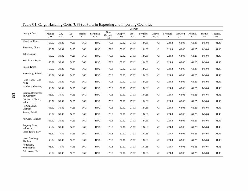
135
Table C1. Cargo Handling Costs (US$) at Ports in Exporting and Importing Countries
Foreign Port
US Port
Mobile
, AL
LA,
CA
LB,
CA
Miami,
FL
Savannah,
GA
New Orleans,
LA
Gulfport
, MS
NY,
NY
Portland,
OR
Charles
ton, SC
Freeport,
TX
Houston
, TX
Norfolk,
VA
Seattle,
WA
Tacoma,
WA
Shanghai, China 68.52 30.32 74.25 36.2 109.2 79.3 52.12 27.12 134.68 42 224.8 63.06 61.25 145.08 91.43
Shenzhen, China 68.52 30.32 74.25 36.2 109.2 79.3 52.12 27.12 134.68 42 224.8 63.06 61.25 145.08 91.43
Tokyo, Japan 68.52 30.32 74.25 36.2 109.2 79.3 52.12 27.12 134.68 42 224.8 63.06 61.25 145.08 91.43
Yokohama, Japan 68.52 30.32 74.25 36.2 109.2 79.3 52.12 27.12 134.68 42 224.8 63.06 61.25 145.08 91.43
Busan, Korea 68.52 30.32 74.25 36.2 109.2 79.3 52.12 27.12 134.68 42 224.8 63.06 61.25 145.08 91.43
Kaohsiung, Taiwan 68.52 30.32 74.25 36.2 109.2 79.3 52.12 27.12 134.68 42 224.8 63.06 61.25 145.08 91.43
Hong Kong, Hong
Kong 68.52 30.32 74.25 36.2 109.2 79.3 52.12 27.12 134.68 42 224.8 63.06 61.25 145.08 91.43
Hamburg, Germany 68.52 30.32 74.25 36.2 109.2 79.3 52.12 27.12 134.68 42 224.8 63.06 61.25 145.08 91.43
Bremen/Bremerhav
en, Germany 68.52 30.32 74.25 36.2 109.2 79.3 52.12 27.12 134.68 42 224.8 63.06 61.25 145.08 91.43
Jawaharlal Nehru,
India 68.52 30.32 74.25 36.2 109.2 79.3 52.12 27.12 134.68 42 224.8 63.06 61.25 145.08 91.43
Ho Chi Minh,
Vietnam 68.52 30.32 74.25 36.2 109.2 79.3 52.12 27.12 134.68 42 224.8 63.06 61.25 145.08 91.43
Santos, Brazil 68.52 30.32 74.25 36.2 109.2 79.3 52.12 27.12 134.68 42 224.8 63.06 61.25 145.08 91.43
Antwerp, Belgium 68.52 30.32 74.25 36.2 109.2 79.3 52.12 27.12 134.68 42 224.8 63.06 61.25 145.08 91.43
Tanjung Priok, Indonesia 68.52 30.32 74.25 36.2 109.2 79.3 52.12 27.12 134.68 42 224.8 63.06 61.25 145.08 91.43
Gioia Tauro, Italy 68.52 30.32 74.25 36.2 109.2 79.3 52.12 27.12 134.68 42 224.8 63.06 61.25 145.08 91.43
Laem Chabang,
Thailand 68.52 30.32 74.25 36.2 109.2 79.3 52.12 27.12 134.68 42 224.8 63.06 61.25 145.08 91.43
Rotterdam,
Netherlands 68.52 30.32 74.25 36.2 109.2 79.3 52.12 27.12 134.68 42 224.8 63.06 61.25 145.08 91.43
Felixstowe, UK 68.52 30.32 74.25 36.2 109.2 79.3 52.12 27.12 134.68 42 224.8 63.06 61.25 145.08 91.43

136
APPENDIX D. CARGO HANDLING CAPACITIES OF THE PANAMA CANAL AND US
PORTS (TEUs)
Table D1. Cargo Handling Capacities of the Panama Canal and US Ports (TEUs)
Port Capacity
Panama Canal 7200000
Mobile, AL 129198
LA, CA 7963333
LB, CA 7583333
Miami, FL 730630
Savannah, GA 2279155
New Orleans, LA 299518
Gulfport, MS 174118
NY, NY 5500000
Portland, OR 156117
Charleston, SC 1166102
Freeport, TX 52704
Houston, TX 1475997
Norfolk, VA 1627311
Seattle, WA 1303482
Tacoma, WA 990938

137
APPENDIX E. INLAND TRANSPORTATION NETWORKS IN THE UNITED STATES

138
Figure E1. Inland Transportation Networks in the United States

139
APPENDIX F. OCEAN TRANSPORTATION NETWORKS IN THE UNITED STATES
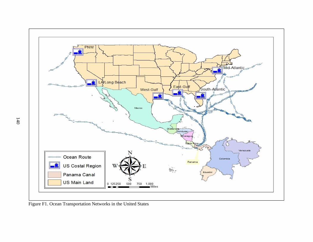
140
Figure F1. Ocean Transportation Networks in the United States

141
APPENDIX G. QUANTITIES OF EXPORTS AND IMPORTS IN 49 STATES OF US
MAINLAND (TEUs)

142
Figure G1. Quantities of Exports and Imports in 49 States of US Mainland (TEUs)

143
APPENDIX H. Q&A FROM PERSONAL INTERVIEW
Interviewee: Mr. Les Koenning, Account Manager and Operations at Osprey Line LLC.
Date: 2 p.m. on July 24th 2014
Question 1: Does your company operate container-on-barge (COB) service as liner along the
US river systems, now?
Answer: No, we used to operate COB as liner service from 1990s to 2000s. We do not
serve COB as liner service since 2009. COB as liner service is no longer
profitable mainly due to the shortage of backhaul because there had not been
enough shipments on the return trip though there was enough shipments for US
imports.
Questions 2: Then, how does your company still operate COB service?
Answer: We serve COB as project which is based on contract.
Question 3: Is there enough demand in the market?
Answer: No, we occasionally have customer for COB.
Question 4: Could you please explain general procedure of COB, now and how do you think
COB services at your company in the future?
Answer: We have our own barge for container which can carry 120 TEUs; however, any
river port facilities have equipment (crane) to handle containers; therefore, we use
crane truck to unload containers. Frankly, in these days, COB has very limited
operation system and infrastructure. I do not think we will be back to COB
service as liner until shipments of COB are balanced.

144
APPENDIX I. GAMS CODE
*this program computes optimal trade flows of containerized shipments
*between the US and its top trade partners in the world. The model is a
*spatial optimization model based on a linear programming algorithm. The objective
*function of the model is to minimize transport costs from shipping origins to destinations via
*various means of transportation modes. The objective function is optimized subject to a
*set of linear constraints.
*Base avg 2011, 2012, 2013
*The model contains containerized shipments regardless of cargo types and value,
*49 shipping origins in the US and 15 importing countries for US exports
*and 49 shipping destinations in the US and 15 exporting countries for US imports,
*15 ports in the US and 18 ports in other countries for US exports and imports,
*and 9 river ports in the US for truck-barge combination.
OPTION limrow=0; OPTION limcol=0;
SETS
I PRODUCING REGIONS IN THE US FOR US EXPORT / ALP, ARP, AZP, CAP, COP, CTP,
DCP, DEP, FLP, GAP,
IAP, IDP, ILP, INP, KSP, KYP, LAP, MAP, MDP, MEP, MIP, MNP, MOP, MSP, MTP, NCP,

145
NDP, NEP, NHP, NJP, NMP, NVP, NYP, OHP, OKP, ORP, PAP, RIP, SCP, SDP, TNP, TXP,
UTP, VAP, VTP, WAP, WIP, WVP, WYP /
A RIVER PORTS IN THE US FOR US EXPORT / ELi, ECh, ELo, EMi, ESt, EKa, ECi, EPi,
EMe /
P SEA PORTS IN THE US / MO, LA, LB, MI, SV, NO, GP, NY, PO, CH, FP, HU, NF, SE, TA
/
Q IMPORT PORTS IN OTHER COUNTRIES FOR US EXPORT / ImCH1, ImCH2, ImJP1,
ImJP2, ImKO, ImTW, ImHK, ImGR1, ImGR2, ImIN, ImVT, ImBR, ImBL, ImID, ImIT, ImTH,
ImNE, ImUK /
D EXPORT PORTS IN OTHER COUNTRIES FOR US IMPORT / ExCH1, ExCH2, ExJP1,
ExJP2, ExKO, ExTW, ExHK, ExGR1, ExGR2, ExIN, ExVT, ExBR, ExBL, ExID, ExIT, ExTH,
ExNE, ExUK /
F RIVER PORTS IN THE US FOR US IMPORT / ILi, ICh, ILo, IMi, ISt, IKa, ICi, IPi, IMe /
G CONSUMTION REGIONS IN THE US FOR US IMPORT / CAL, CAR, CAZ, CCA, CCO,
CCT, CDC, CDE, CFL, CGA,
CIA, CID, CIL, CIN, CKS, CKY, CLA, CMA, CMD, CME, CMI, CMN, CMO, CMS, CMT,
CNC, CND, CNE,
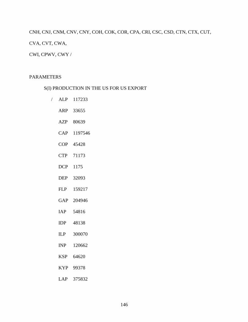
146
CNH, CNJ, CNM, CNV, CNY, COH, COK, COR, CPA, CRI, CSC, CSD, CTN, CTX, CUT,
CVA, CVT, CWA,
CWI, CPWV, CWY /
PARAMETERS
S(I) PRODUCTION IN THE US FOR US EXPORT
/ ALP 117233
ARP 33655
AZP 80639
CAP 1197546
COP 45428
CTP 71173
DCP 1175
DEP 32093
FLP 159217
GAP 204946
IAP 54816
IDP 48138
ILP 300070
INP 120662
KSP 64620
KYP 99378
LAP 375832
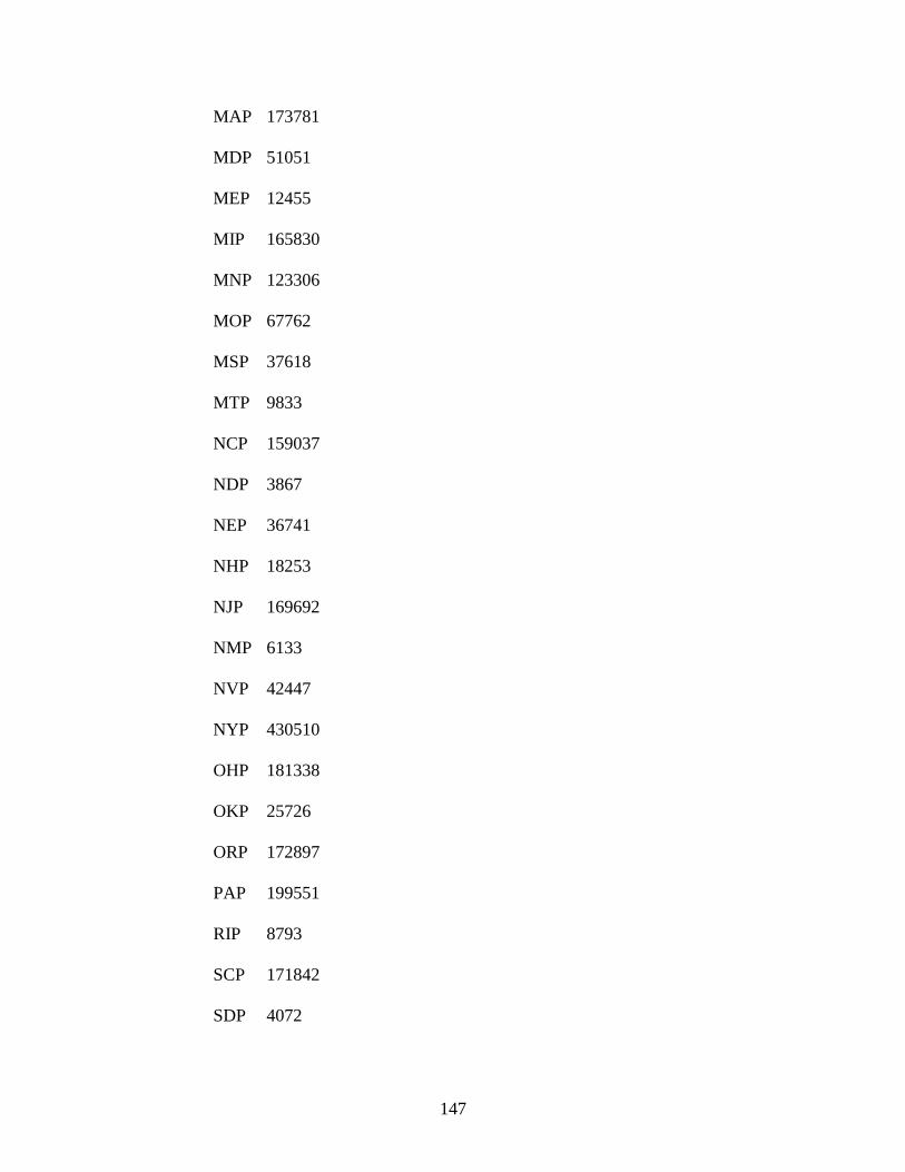
147
MAP 173781
MDP 51051
MEP 12455
MIP 165830
MNP 123306
MOP 67762
MSP 37618
MTP 9833
NCP 159037
NDP 3867
NEP 36741
NHP 18253
NJP 169692
NMP 6133
NVP 42447
NYP 430510
OHP 181338
OKP 25726
ORP 172897
PAP 199551
RIP 8793
SCP 171842
SDP 4072

148
TNP 147655
TXP 860711
UTP 139019
VAP 110890
VTP 28887
WAP 684682
WIP 94642
WVP 60581
WYP 6828 /
T(P) PORT CAPACITY IN THE US
/ MO 129198
LA 7963333
LB 7583333
MI 730630
SV 2279155
NO 299518
GP 174118
NY 5500000
PO 156117
CH 1166102
FP 52704
HU 1475997

149
NF 1627311
SE 1303482
TA 990938 /
U(Q) CONSUMPTION IN IMPORTING COUNTRY FOR US EXPORT
/ ImCH1 1363375
ImCH2 1363375
ImJP1 407336
ImJP2 407336
ImKO 649634
ImTW 590242
ImHK 389609
ImGR1 129087
ImGR2 129087
ImIN 333245
ImVT 192100
ImBR 303954
ImBL 271840
ImID 213618
ImIT 116547
ImTH 142542
ImNE 201060
ImUK 209061 /

150
J(D) PRODUCTION IN OTHER COUNTRIES FOR US IMPORT
/ ExBL 266367
ExBR 279279
ExCH1 4313660
ExCH2 4313660
ExGR1 274052
ExGR2 274052
ExHK 452968
ExIN 438508
ExID 308421
ExIT 368599
ExJP1 309902
ExJP2 309902
ExNE 223395
ExKO 695674
ExTW 525462
ExTH 336851
ExUK 187116
ExVT 555145 /
K(G) COMSUMPTION IN THE US FOR US IMPORT
/ CAL 136500

151
CAR 57135
CAZ 95432
CCA 3699245
CCO 68940
CCT 117991
CDC 2115
CDE 45775
CFL 441257
CGA 618495
CIA 44962
CID 37081
CIL 828092
CIN 222822
CKS 89173
CKY 260064
CLA 98608
CMA 176948
CMD 151541
CME 14753
CMI 259628
CMN 244621
CMO 119956
CMS 101813

152
CMT 3701
CNC 351987
CND 6898
CNE 27299
CNH 32504
CNJ 751093
CNM 20890
CNV 89418
CNY 1071657
COH 411269
COK 65122
COR 120697
CPA 534309
CRI 55348
CSC 240064
CSD 4857
CTN 611252
CTX 1354621
CUT 47728
CVA 168112
CVT 10174
CWA 317032
CWI 185985

153
CPWV 15071
CWY 2977 /
*Read the following data from C-drive
TABLE IT1(I,A) SHIPPING RATE FROM PRODUCTUIN REGION TO RIVER PORT BY
TRUCK (USD)
$include "C:\Users\Jude\Desktop\GAMS\New
Table\Base_Model\TFR_US_Export_to_BAP_Base_250.txt" ;
TABLE IT2(I,P) SHIPPING RATE FROM PRODUCTION REGION TO EXPORT PORT BY
TRUCK (USD)
$include "C:\Users\Jude\Desktop\GAMS\New
Table\Base_Model\TFR_US_Export_to_ESP_Base_250.txt" ;
TABLE IB(A,P) SHIPPING RATE FROM RIVER PORT TO EXPORT PORT BY BARGE
(USD)
$include "C:\Users\Jude\Desktop\GAMS\New
Table\Base_Model\BFR_US_Export_Base_250.txt" ;
TABLE NG3(A,P) NO-GO MATRIX
$include "C:\Users\Jude\Desktop\GAMS\New Table\Base_Model\ng3_01.txt" ;

154
TABLE IR(I,P) SHIPPING RATE FROM PRODUCTION REGION TO EXPORT PORT BY
RAIL (USD)
$include "C:\Users\Jude\Desktop\GAMS\New
Table\Base_Model\RFR_US_Export_Base_250_01.txt" ;
TABLE OT1(P,Q) SHIPPING RATE FROM EXPORT PORT TO IMPORT PORT WITHOUT
PNC BY VESSEL (USD)
$include "C:\Users\Jude\Desktop\GAMS\New
Table\Base_Model\OFR_US_Export_no_PNC_01.txt" ;
TABLE NG5(P,Q) NO-GO MATRIX
$include "C:\Users\Jude\Desktop\GAMS\New Table\Base_Model\ng5_01.txt" ;
TABLE OT2(P,Q) SHIPPING RATE FROM EXPORT PORT TO IMPORT PORT VIA PNC
BY VESSEL (USD)
$include "C:\Users\Jude\Desktop\GAMS\New
Table\Base_Model\OFR_US_Export_thu_PNC_01.txt" ;
TABLE NG6(P,Q) NO-GO MATRIX
$include "C:\Users\Jude\Desktop\GAMS\New Table\Base_Model\ng6_01.txt" ;
TABLE TC(P,Q) TERMINAL HANDLING CHARGE AT EXPORT AND IMPORT PORT
FOR US EXPORT (USD)
155
$include "C:\Users\Jude\Desktop\GAMS\New Table\Base_Model\ESP_THC_01.txt" ;
TABLE PT(P,Q) PANAMA CANAL TOLL RATE FOR US EXPORT (USD)
$include "C:\Users\Jude\Desktop\GAMS\New Table\Base_Model\US_Ex_PNC_TOL_01.txt" ;
TABLE PH(P,Q) PANAMA CANAL HANDLING CHARGE FOR US EXPORT (USD)
$include "C:\Users\Jude\Desktop\GAMS\New Table\Base_Model\US_Ex_PNC_THC_01.txt" ;
TABLE PD(P,Q) PANAMA CANAL DELAY COST FOR US EXPORT (USD)
$include "C:\Users\Jude\Desktop\GAMS\New Table\Base_Model\US_Ex_PNC_DEL_01.txt" ;
TABLE OTI1(D,P) SHIPPING RATE FROM FOREIGN EXPORT PORT TO US IMPORT
PORT WITHOUT PNC BY VESSEL (USD)
$include "C:\Users\Jude\Desktop\GAMS\New
Table2\Base_Model\OFR_USIMPORT_NO_PNC_01.txt" ;
TABLE NG12(D,P) NO-GO MATRIX
$include "C:\Users\Jude\Desktop\GAMS\New Table2\Base_Model\ng12_01.txt" ;
TABLE OTI2(D,P) SHIPPING RATE FROM FOREIGN EXPORT PORT TO US IMPORT
PORT VIA PNC BY VESSEL (USD)
$include "C:\Users\Jude\Desktop\GAMS\New
Table2\Base_Model\OFR_USIMPORT_thu_PNC_01.txt" ;

156
TABLE NG13(D,P) NO-GO MATRIX
$include "C:\Users\Jude\Desktop\GAMS\New Table2\Base_Model\ng13_01.txt" ;
TABLE IBI(P,F) SHIPPING RATE FROM US IMPORT PORT TO US IMPORT RIVER
PORT BY BARGE (USD)
$include "C:\Users\Jude\Desktop\GAMS\New
Table2\Base_Model\BFR_US_Import_Base_250.txt" ;
TABLE NG9(P,F) NO-GO MATRIX
$include "C:\Users\Jude\Desktop\GAMS\New Table2\Base_Model\ng9_01.txt" ;
TABLE ITI1(F,G) SHIPPING RATE FROM US IMPORT RIVER PORT TO US
CONSUMPTION REGION BY TRUCK (USD)
$include "C:\Users\Jude\Desktop\GAMS\New
Table2\Base_Model\TFR_US_Import_from_BAP_Base_250.txt" ;
TABLE ITI2(P,G) SHIPPING RATE FROM US IMPORT PORT TO US CONSUMPTION
REGION BY TRUCK (USD)
$include "C:\Users\Jude\Desktop\GAMS\New
Table2\Base_Model\TFR_US_Import_from_ISP_Base_250.txt" ;

157
TABLE IRI(P,G) SHIPPING RATE FROM US IMPORT PORT TO US CONSUMPTION
REGION BY RAIL (USD)
$include "C:\Users\Jude\Desktop\GAMS\New
Table2\Base_Model\RFR_US_Import_Base_250_01.txt" ;
TABLE TCI(D,P) TERMINAL HANDLING CHARGE AT EXPORT AND IMPORT PORT
FOR US IMPORT (USD)
$include "C:\Users\Jude\Desktop\GAMS\New Table2\Base_Model\US_IMP_THC_01.txt" ;
TABLE PTI(D,P) PANAMA CANAL TOLL RATE FOR US IMPORT (USD)
$include "C:\Users\Jude\Desktop\GAMS\New Table2\Base_Model\US_IM_PNC_TOL_01.txt" ;
TABLE PHI(D,P) PANAMA CANAL HANDLING CHARGE FOR US IMPORT (USD)
$include "C:\Users\Jude\Desktop\GAMS\New Table2\Base_Model\US_IM_PNC_THC_01.txt" ;
TABLE PDI(D,P) PANAMA CANAL DELAY COST FOR US IMPORT (USD)
$include "C:\Users\Jude\Desktop\GAMS\New Table2\Base_Model\US_IM_PNC_DEL_01.txt" ;

158
PARAMETERS
IT1(I,A) TRUCK FREIGHT RATE FROM I TO A IN DOLLARS
IT2(I,P) TRUCK FREIGHT RATE FROM I TO P IN DOLLARS
IB(A,P) BARGE FREIGHT RATE FROM A TO P IN DOLLARS
IR(I,P) RAIL FREIGHT RATE FROM I TO P IN DOLLARS
OT1(P,Q) OCEAN FREIGHT RATE FROM P TO Q WITHOUT PNC IN DOLLARS
OT2(P,Q) OCEAN FREIGHT RATE FROM P TO Q VIA PNC IN DOLLARS
TC(P,Q) TERMINAL HANDLING CHARGE AT PORT FOR US EXPORT
PT(P,Q) PANAMA CANAL TOLL FOR US EXPORT IN DOLLARS
PH(P,Q) PANAMA CHNAL HANDLING CHARGE FOR US EXPORT IN
DOLLARS
PD(P,Q) PANAMA CHNAL DELAY COST FOR US EXPORT IN DOLLARS
OTI1(D,P) OCEAN FREIGHT RATE FROM D TO E WITHOUT PNC IN DOLLARS
OTI2(D,P) OCEAN FREIGHT RATE FROM D TO E VIA PNC IN DOLLARS
IBI(P,F) BARGE FREUGHT RATE FROM E TO F IN DOLLARS
ITI1(F,G) TRUCK FREIGHT RATE FROM F TO G IN DOLLARS
ITI2(P,G) TRUCK FREIGHT RATE FROM E TO G IN DOLLARS
IRI(P,G) RAIL FREIGHT RATE FROM E TO G IN DOLLARS
TCI(D,P) TERMINAL HANDLING CHARGE AT PORT FOR US IMPORT
PTI(D,P) PANAMA CANAL TOLL IN DOLLARS FOR US IMPORT
PHI(D,P) PANAMA CHNAL HANDLING CHARGE FOR US EXPORT IN
DOLLARS
PDI(D,P) PANAMA CANAL DELAY COST FOR US IMPORT (USD) ;

159
VARIABLES
costs
x(I,A) QUANTITY FROM PRODUCING REGION TO RIVER PORT
m(A,P) QUANTITY FROM RIVER PORT TO EXPORT PORT
n(I,P) QUANTITY FROM PRODUCING REGION TO EXPORT PORT
o(P,Q) QUANTITY FROM EXPORT PORT TO IMPORT PORT WITHOUT
PNC
r(P,Q) QUANTITY FROM EXPORT PORT TO IMPORT PORT VIA PNC
h1(D,P) QUANTITY FROM PRODUCING COUNTRY TO US IMPORT PORT
WITHOUT PNC FOR US IMPORT
h5(D,P) QUANTITY FROM PRODUCING COUNTRY TO US IMPORT PORT
VIA PNC FOR US IMPORT
h2(P,F) QUANTITY FROM US IMPORT PORT TO US IMPORT RIVER PORT
h3(F,G) QUANTITY FROM US IMPORT RIVER PORT TO CONSUMING
REGION
h4(P,G) QUANTITY FROM US IMPORT PORT TO CONSUMING REGION
POSITIVE VARIABLES x, m, n, o, r, h1, h2, h3, h4, h5 ;
EQUATIONS
Obj costs
SUPPLY(I) OBSERVE SUPPLY LIMIT AT PRODUCING REGION I
160
DEMAND(Q) SATISFY DEMAND AT IMPORTING COUNTRY Q
PORTBALANCE1(A) RIPORT CLEARING
PORTBALANCE2(P) EXPORT CLEARING
ISUPPLY(D) OBSERVE SUPPLY LIMIT AT PRODUCING REGION D
IDEMAND(G) SATISFY DEMAND IN THE US G
IPORTBALANCE1(P) IMPORT CLEARING
IPORTBALANCE2(F) IRIPORT CLEARING
PORTCAP(P) PORT CAPACITY
PNCAP PNC CAPACITY ;
obj.. costs =E= SUM((I,A),x(I,A) * IT1(I,A))
+ SUM((A,P),m(A,P) * IB(A,P))
+ SUM((I,P),n(I,P) * IT2(I,P))
+ SUM((I,P),n(I,P) * IR(I,P))
+ SUM((P,Q),o(P,Q) * (OT1(P,Q) + TC(P,Q)))
+ SUM((P,Q),r(P,Q) * (OT2(P,Q) + TC(P,Q)
+ PT(P,Q) + PH(P,Q) + PD(P,Q)))
+ SUM((D,P),h5(D,P) * (OTI2(D,P) + TCI(D,P)
+ PTI(D,P) + PHI(D,P) + PDI(D,P)))
+ SUM((D,P),h1(D,P) * (OTI1(D,P) + TCI(D,P)))
+ SUM((P,F),h2(P,F) * IBI(P,F))
+ SUM((F,G),h3(F,G) * ITI1(F,G))
+ SUM((P,G),h4(P,G) * ITI2(P,G))

161
+ SUM((P,G),h4(P,G) * IRI(P,G)) ;
SUPPLY(I).. SUM(A,x(I,A)) + SUM(P,n(I,P)) =L= S(I) ;
DEMAND(Q).. SUM(P,o(P,Q)) + SUM(P,r(P,Q)) =G= U(Q) ;
PORTBALANCE1(A).. SUM(I,x(I,A)) =E= SUM(P,m(A,P)) ;
PORTBALANCE2(P).. SUM(A,m(A,P)) + SUM(I,n(I,P)) =E= SUM(Q,o(P,Q)) +
SUM(Q,r(P,Q)) ;
ISUPPLY(D).. SUM(P,h1(D,P)) + SUM(P,h5(D,P)) =L= J(D) ;
IDEMAND(G).. SUM(F,h3(F,G)) + SUM(P,h4(P,G)) =G= K(G) ;
IPORTBALANCE1(P).. SUM(D,h1(D,P)) + SUM(D,h5(D,P)) =E= SUM(F,h2(P,F)) +
SUM(G,h4(P,G)) ;
IPORTBALANCE2(F).. SUM(P,h2(P,F)) =E= SUM(G,h3(F,G)) ;
PORTCAP(P).. SUM(A,m(A,P)) + SUM(I,n(I,P)) + SUM(D,h1(D,P)) + SUM(D,h5(D,P))
=L= T(P) ;

162
PNCAP.. SUM((P,Q),r(P,Q)) + SUM((D,P),h5(D,P)) =L= 7200000 ;
Loop((A,P)$(NG3(A,P)EQ 0),
m.fx(A,P)=0 ;
);
Loop((P,Q)$(NG5(P,Q)EQ 0),
o.fx(P,Q)=0 ;
);
Loop((P,Q)$(NG6(P,Q)EQ 0),
r.fx(P,Q)=0 ;
);
Loop((D,P)$(NG12(D,P)EQ 0),
h1.fx(D,P)=0 ;
);
Loop((D,P)$(NG13(D,P)EQ 0),
h5.fx(D,P)=0 ;
);

163
Loop((P,F)$(NG9(P,F)EQ 0),
h2.fx(P,F)=0 ;
);
MODEL TRANSPORT /ALL/;
SOLVE TRANSPORT USING LP MINIMIZING costs ;
FILE out /C:\Users\Jude\Desktop\GAMS\Test\Base_Model_Final.prn/;
put out;
put "Trade flows from PROD Region to River Port for US Export"
put /;
loop((I,A)$x.l(I,A),
put I.tl,A.tl,x.l(I,A)
put /;
);
put "Trade flows from River Port to Export Port for US Export"
put /;
loop((A,P)$m.l(A,P),
put A.tl,P.tl,m.l(A,P)
put /;

164
);
put "Trade flows from PROD Region to Export Port for US Export"
put /;
loop((I,P)$n.l(I,P),
put I.tl,P.tl,n.l(I,P)
put /;
);
put "Trade flows from Export Port to Import Port without PNC for US Export"
put /;
loop((P,Q)$o.l(P,Q),
put P.tl,Q.tl,o.l(P,Q)
put /;
);
put "Trade flows from Export Port to Import Port via PNC for US Export"
put /;
loop((P,Q)$r.l(P,Q),
put P.tl,Q.tl,r.l(P,Q)
put /;
);
165
put "Trade flows from PROD Country to US Import Port without PNC for US Import"
put /;
loop((D,P)$h1.l(D,P),
put D.tl,P.tl,h1.l(D,P)
put /;
);
put "Trade flows from PROD Country to US Import Port via PNC for US Import"
put /;
loop((D,P)$h5.l(D,P),
put D.tl,P.tl,h5.l(D,P)
put /;
);
put "Trade flows from US Import port to US Import river port for US Import"
put /;
loop((P,F)$h2.l(P,F),
put P.tl,F.tl,h2.l(P,F)
put /;
);
put "Trade flows from US Import river port to consuming region for US Import"
put /;

166
loop((F,G)$h3.l(F,G),
put F.tl,G.tl,h3.l(F,G)
put /;
);
put "Trade flows from US Import port to consuming region for US Import"
put /;
loop((P,G)$h4.l(P,G),
put P.tl,G.tl,h4.l(P,G)
put /;
);