Impact of the Cardiac Heart Flow Alpha Project

Kathy YelickEECS Department

U.C. Berkeley

Outline

• Vision of a Digital Human• Applications of the IBM

– The Heart Model– The Cochlea Model– Others

• Overview of the Immersed Boundary Method

• The Alpha project– Solvers– Automatic tuning (FFT vs. MG)– Heart model

• Short term future directions

Simulation: The Third Pillar of Science • Traditional scientific and engineering

paradigm:1) Do theory or paper design.2) Perform experiments or build system.

• Limitations:– Too difficult -- build large wind tunnels.– Too expensive -- build a throw-away passenger jet.– Too slow -- wait for climate or galactic evolution.– Too dangerous -- drug design.

• Computational science paradigm:3) Use high performance computer systems

to simulate the phenomenon.

Economics of Large Scale Simulation• Automotive design:

– Crash and aerodynamics simulation (500+ CPUs).– Savings: approx. $1 billion per company per year.

• Semiconductor industry:– Device simulation and logic validation (500+ CPUs).– Savings: approx. $1 billion per company per year.

• Airlines:– Logistics optimization on parallel system.– Savings: approx. $100 million per airline per year.

• Securities industry:– Home mortgage investment and risk analysis.– Savings: approx. $15 billion per year.

• What about health care, which is 20% of GNP?Source: David Bailey, LBNL

From Visible Human to Digital Human

Source: John Sullivan et al, WPI

Source: www.madsci.org

Building 3D Models from images

Heart Simulation Calculation

Developed by Peskin and McQueen at NYU– Done on a Cray C90: 1 heart-beat in 100 hours– Used for evaluating artificial heart valves– Scalable parallel version done here

• Implemented in a high performance Java dialect

–Model also used for: • Inner ear

• Blood clotting

• Embryo growth

• Insect flight

• Paper making

Simulation of a Heart

Simulation and Medicine

• Imagine a “digital body double” – 3D image-based medical record– Includes diagnostic, pathologic, and other

information

• Used for:– Diagnosis– Less invasive surgery-by-robot– Experimental treatments

Where are we today?

Digital Human Roadmap

1995 2000 2005 2010

1 organ 1 model

scalable implementations

1 organ multiple models

multiple organs

3D model construction

better algorithms

organ system

coupled models

100x effective performance

improved programmability

Last Year

Project Summary

• Provide easy-to-use, high performance tool for simulation of fluid flow in biological systems.– Using the Immersed Boundary Method

• Enable simulations on large-scale parallel machines. – Distributed memory machine including SMP

clusters

• Using Titanium, ADR, and KeLP with AMR• Specific demonstration problem: Simulation

of the heart model on Blue Horizon.

Outline

• Short term goals and plans• Technical status of project

– Immersed Boundary Method– Software Tools– Solvers

• Next Steps

Short Term Goals for October 2001IB Method written in Titanium (IBT)IBT Simulation on distributed memoryHeart model input and visualization

support in IBTTitanium running on Blue Horizon• IBT users on BH and other SPs? Performance tuning of code to exceed

T90 performance? Replace solver with (adaptive)

multigrid

IB Method Users• Peskin and McQueen at NYU

– Heart model, including valve design

• At Washington– Insect flight

• Fauchy et al at Tulane– Small animal swimming

• Peter Kramer at RPI– Brownian motion in the IBM

• John Stocky at Simon Fraser– Paper making

• Others– parachutes, flags, flagellates, robot insects

Building a User Community

• Many users of the IB Method• Lots of concern over lack of

distributed memory implementation• Once IBT is more robust and efficient

(May ’01), advertise to users• Identify 1 or 2 early adopters

• Longer term: workshop or short course

Long Term Software Release Model

• Titanium– Working with UPC and possibly others

on common runtime layer– Compiler is relatively stable but needs

ongoing support

• IB Method– Release Titanium source code– Parameterized “black box” for IB

Method with possible cross-language support

• Visualization software is tied to SGI

Immersed Boundary Method

• Developed at NYU by Peskin & McQueen to model biological systems where elastic fibers are immersed in an incompressible fluid. – Fibers (e.g., heart muscles) modeled

by list of fiber points– Fluid space modeled by a regular

lattice

Immersed Boundary Method Structure

Fiber activation & force calculation

InterpolateVelocity

Navier-Stokes Solver

SpreadForce

4 steps in each timestep

Fiber Points

Interaction

Fluid Lattice

Challenges to Parallelization• Irregular fiber lists need to interact

with regular fluid lattice. – Trade-off between load balancing of

fibers and minimizing communication• Efficient “scatter-gather” across processors

• Need a scalable elliptic solver– Plan to uses multigrid – Eventually add Adaptive Mesh

Refinement• New algorithms under development by

Colella’s group

Tools used for Implementation• Titanium supports

– Classes, linked data structures, overloading– Distributed data structures (global address

space)– Useful for planned adaptive hierarchical

structures

• ADR provides– Help with analysis and organization of output– Especially for hierarchical data

• KeLP provides– Alternative programming model for solvers

• ADR and KeLP are not critical for first-year

Titanium Status

• Titanium runs on uniprocessors, SMPs, and distributed memory with a single programming model

• It has run on Blue Horizon– Issues related to communication

balance– Revamped backends are more

organized, but BH backend not working right now

• Need to replace personnel

Solver Status

• Current solver is based on 3D FFT• Multigrid might be more scalable• Multigrid with adaptive meshes might be

more so• Balls and Colella algorithm could also be

used• KeLP implementations of solvers included• Note: McQueen is looking into solver issues

for numerical reasons unrelated to scaling• Not critical for first year goals

IB Titanium Status

• IB (Generic) rewritten in Titanium.

• Running since October

• Contractile torus– runs on Berkeley NOW

and SGI Origin

• Needed for heart: – Input file format – Performance tuning

•Uniprocessor (C code used temporarily in 2 kernels)

•Communication

Immersed Boundary on Titanium

• Performance Breakdown (torus simulation):

Berkeley NOW, 4 processors

NS Solver44%

Interpolate Velocity

39%

Fiber Calculation

0%

Spread Force27%

Argonne Lab SGI Origin, 4 processors

NS Solver30%

Interpolate Velocity

34%

Fiber Calculation

2%

Spread Force34%

Immersed Boundary on Titanium

Relative speedup on the NOW

00.5

11.5

22.5

33.5

44.5

5

1 2 4 8Number of processors

Speedup

FiberCalculation

SpreadForce

Fluid Solver

InterpolateVelocity

Overall

Next Steps

• Improve performance of IBT• Generate heart input for IBT• Recover Titanium on BH• Identify early user(s) of IBT• Improve NS solver• Add functionality

– Bending angles, anchorage points, source & sinks) to the software package.

Yelick(UCB), Peskin (NYU), Colella (LBNL), Baden (UCSD),

Saltz (Maryland)

Adaptive Computations for

Fluids in Biological Systems

Immersed BoundaryMethod Applications

Human Heart (NYU)

Embryo Growth (UCB)

Blood Clotting (Utah)

Robot Insect Flight (NYU)

Pulp Fibers (Waterloo)

Generic Immersed Boundary Method (Titanium)

Heart(Titanium)

InsectWings

FlagellateSwimming

…

Spectral(Titanium)

Multigrid(KeLP)

AMR

Application Models

Extensible Simulation

Solvers

General Questions• - How has your project addressed the goals of the PACI program (providing

access to tradition HPC, providing early access to experimental systems,fostering interdisciplinary research, contributing to intellectualdevelopment, broadening the base)?- What infrastructure products (e.g., software, algorithms, etc.) have you produced?- Where have you deployed them (on NPACI systems, other systems)?- What have you done to communicate the availability of thisinfrastructure?- What training have you done?- What kind/size of community is using your infrastructure?- How have you integrated your work with EOT activities?- What scientific accomplishments - or other measurable impacts notcovered by answers to previous questions - have resulted from its use?- What are the emerging trends/technologies that NPACI should buildon/leverage?- How can we increase the impact of NPACI development to date?- How can we increase the community that uses the infrastructure you'vedeveloped?

Greg’s Slides

Scallop

• A latency tolerant elliptical solver library

• Implemented in KeLP, with a simple interface

• Still under development

Elliptical solvers

• A finite-difference based solvers– Good for regular, block-structured

domains• Method of Local Corrections

– Local solutions corrected by a coarse solution

– Good accuracy, well-conditioned solutions

• Limited communication– Once to generate coarse grid values– Once to correct local solutions

KeLP implementation

• Advantages – abstractions available in C++– built in domain calculus– communication management– numerical kernels written in Fortran

• Simple interface– callable from other languages– no KeLP required in user code

A Finite Difference Domain Decomposition Method Using Local Corrections for the Poisson Equation

Greg BallsUniversity of California, Berkeley

The Poisson Equation

• We are interested in the solution to

• A particular solution to this equation is

2 of all on,

zzGydyyxG 1

log21

)(,)()(

Infinite Domain Boundary Conditions

• We can write our infinite domain boundary condition as

• These boundary conditions specify a unique solution.

xox

R ),1(1

log2

xdxR )(

The Discretized Problem

• We would like an approximate solution

1,01,0)supp(

),(, jhihexactji

NhNji

1,,0

Solving the Discretized Problem

• We could calculate the convolution integral at each point

• Multigrid provides a faster method work)( 4NO

work)log( 2 NNO

A Standard Finite Difference Discretization

• With a discretization of the Laplacian, e.g.

• We solve the discretized equation

jijijijijiji hL ,1,1,,1,12,

5 41

),(, jhihL ji

1,11,11,11,12,9

61

jijijijiji hL

jijijijiji ,1,1,,1,1 204

A Finite Difference Approach for the Infinite Domain Problem

• A discrete solution can be found in three steps:

1. Solve a multigrid problem with homogeneous Dirichlet boundary conditions.

2. Do a potential calculation to set accurate inhomogeneous Dirichlet boundary conditions.

3. Solve a second multigrid problem with these boundary conditions.

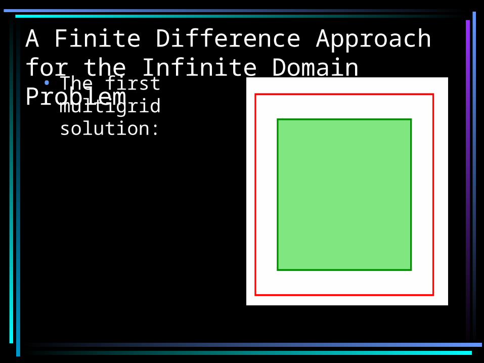
A Finite Difference Approach for the Infinite Domain Problem

• The first multigrid solution:

DDL on

DD on0

A Finite Difference Approach for the Infinite Domain Problem

• The potential calculation:

dssyxGsyxP

inside

D

nsy

sy

A Finite Difference Approach for the Infinite Domain Problem

• The second multigrid solution:

BBL on

BPB on

Domain Decomposition

• We would like to solve this problem in parallel, calculating h such that

• A basic domain decomposition strategy:Do until converged -

• Break into pieces.• Solve on each piece.• Compute coupling.

2hOexacth

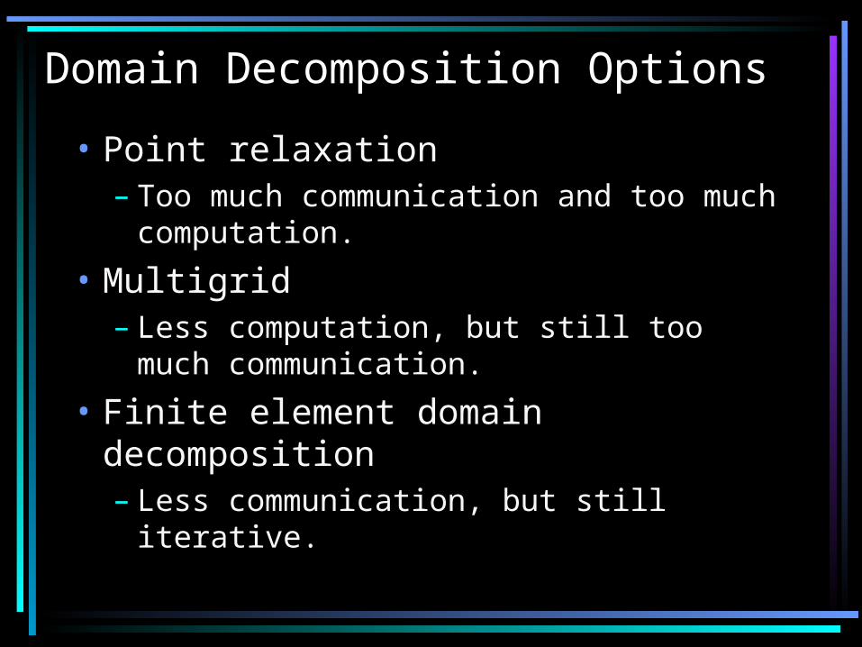
Domain Decomposition Options

• Point relaxation– Too much communication and too

much computation.

• Multigrid– Less computation, but still too much

communication.

• Finite element domain decomposition– Less communication, but still iterative.

The Importance of Communication

• Current parallel machines can do many floating point operations in the time that it takes to send a message.

• This imbalance will get worse.

Fast Particle Methods

• Methods such as FMM and MLC need no iteration.

• They take advantage of the fact that the local and far-field solutions are only weakly coupled.

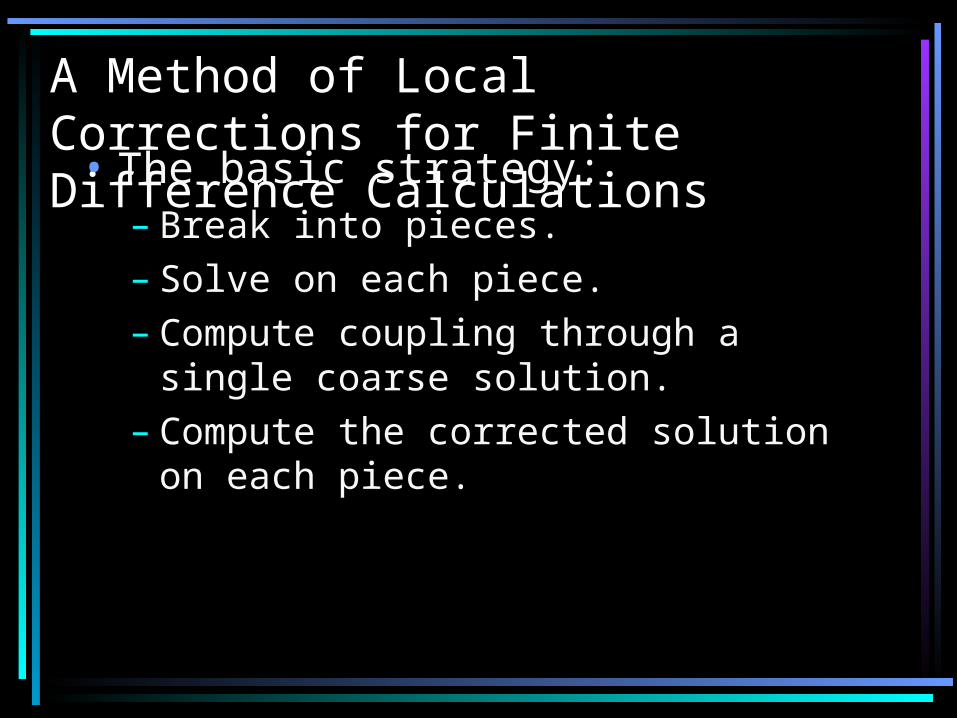
A Method of Local Corrections for Finite Difference Calculations

• The basic strategy:– Break into pieces.– Solve on each piece.– Compute coupling through a single

coarse solution.– Compute the corrected solution on

each piece.

The Initial Solution

• An infinite domain solution is found on each piece, l

• The effects of all other pieces are ignored.

hl

initialhlL ,9

A Coarse Grid Charge

• A coarse grid charge is computed for each piece.

initialHl

Hl L ,9

initialhl

initialHl A ,,

The Global Coarse Solution

• All the individual coarse grid charges are combined on a global coarse grid.

• A global coarse solution is found.

HHL 9

l

Hl

H

Setting Accurate Boundary Conditions

• The interpolation stencil only interpolates far-field information.

stencilHH

mm

initialHm

HstencilH

,:

,,

Hk

Hj

Setting Accurate Boundary Conditions

• The coarse stencil information is interpolated to a corresponding fine grid stencil to O(H4).

• Local information is added from nearby fine grids.

stencilHHm

lm

initialhm

stencilhhl

,:

,,

The Corrected Solution

• Once the boundary conditions have been set for each piece, we solve one last time with multigrid:

• The full solution is thenhl

hlL 5

l

hl

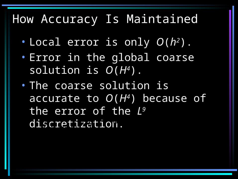
How Accuracy Is Maintained

• Local error is only O(h2).• Error in the global coarse solution

is O(H4).• The coarse solution is accurate to O(H4) because of the error of the L9 discretization.

where),( 64)supp(~

HOHexact H

0H

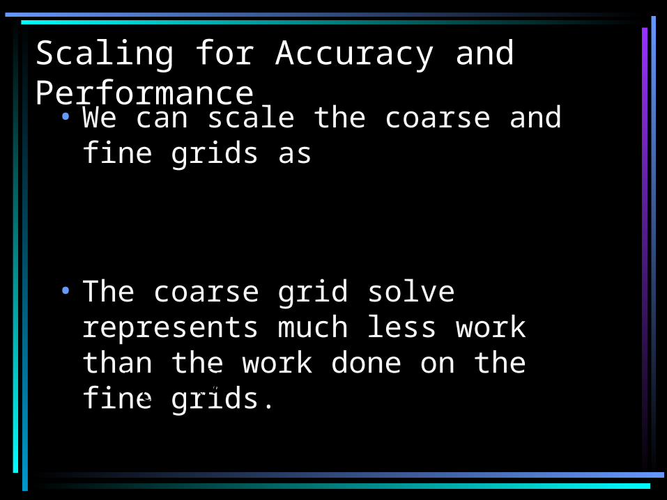
Scaling for Accuracy and Performance

• We can scale the coarse and fine grids as

• The coarse grid solve represents much less work than the work done on the fine grids.

hOH

NNC

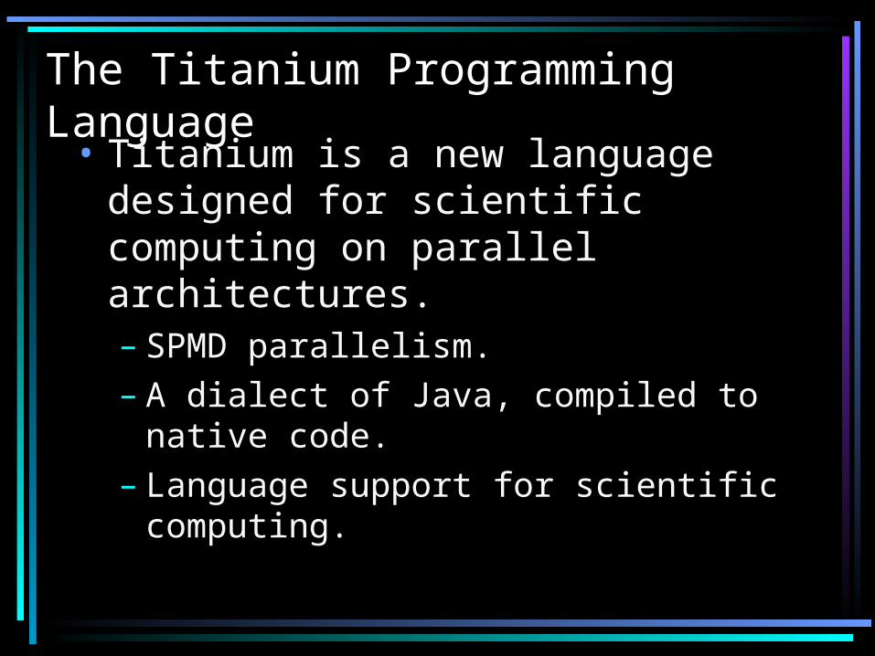
The Titanium Programming Language

• Titanium is a new language designed for scientific computing on parallel architectures.– SPMD parallelism.– A dialect of Java, compiled to native

code.– Language support for scientific

computing.

The Benefits of Titanium

• An object-oriented language with built-in support for fast, multi-dimensional arrays.

• Language support for– Tuples (Points).– Rectangular regions (RectDomains).– Expressing array bounds as

RectDomains and indexing arrays by Points.

• A global address space

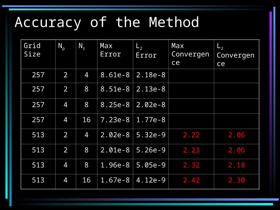
Accuracy of the Method

Grid Size

Np Nr Max Error

L2 Error Max Convergence

L2 Convergence

257 2 4 8.61e-8 2.18e-8

257 2 8 8.51e-8 2.13e-8

257 4 8 8.25e-8 2.02e-8

257 4 16 7.23e-8 1.77e-8

513 2 4 2.02e-8 5.32e-9 2.22 2.06

513 2 8 2.01e-8 5.26e-9 2.23 2.06

513 4 8 1.96e-8 5.05e-9 2.32 2.18

513 4 16 1.67e-8 4.12e-9 2.42 2.30

Error on a Large, High-Wavenumber Problem

91047.6

91031.1

Scalability of the Method

• Results from the SDSC IBM SP-2:

Scalability of the Method

• Results from the NERSC Cray T3E:

Future Work

• Extension to three dimensions.• Implementation of different

boundary conditions.• Use in other solvers such as:

– Euler.– Navier-Stokes.

Conclusions

• The method is second-order accurate.

• The method does not iterate between the local fine representations and the global coarse grid.

• The need for communication is kept to a minimum.

• The method is scalable.

Comparison to the Serial Method

• Extra computational costs:– The time spent on the coarse grid

solution can be kept to less than 10% of time spent on the local fine grids.

– The final multigrid solution adds 40% more fine grid work.

• Communication costs:– Experimentally, less than 1% of the

total time