impact of mobility on last encounter routing protocolshelmy/papers/maid-secon... · this research...

Impact of Mobility on Last Encounter RoutingProtocols

Fan Bai*, Ahmed Helmy** General Motors Research Center, General Motors Corporation

tComputer and Information Science and Engineering Department, University of Florida

Abstract- In this study, we analyze last encounter basedrouting protocol (e.g., FResher Encounter SearcH, orFRESH) that utilizes encounter history to create time(or age) gradients for information diffusion in wirelessnetworks. FRESH protocols can be used for resourcediscovery, routing or node location, and hold great promisefor future wireless networks.We provide the first study on sensitivity of this class

of protocols to a rich set of mobility models (Manhattan,Group, Random Walk and Random Waypoint models).We find that FRESH is sensitive to the mobility pattern.However, somewhat to our surprise, FRESH's performanceafter warm-up is insensitive to velocity for all the mobilitymodels examined. To expose the fundamental reason be-hind these observations, we develop analytical models toanalyze FRESH's performance and validate these modelsvia extensive simulations. Finally, our analysis concludesthat the characteristics of the age gradient tree is the keyfactor to explain this interplay between mobility and theperformance of FRESH protocols.

I. INTRODUCTION

Recent studies [6] [7] indicate that mobility im-poses negative effects on conventional routing protocols(e.g., DSR, AODV, DSDV, etc.). However, mobilityalso provides opportunities that can, and in fact should,be utilized to enhance the performance of MANETprotocols. For example, last encounter based protocols(e.g., EASE [5], or FRESH [4]) explicitly use the nodemobility and encounter history to locate (and establishroutes to) other nodes. In this paper, we focus on FRESHprotocol [4], as a generic example for this type of lastencounter based protocols. FRESH uses node encounterhistory to create time (encounter age) gradient tree withinthe network. By following the time (or age) gradient, amobile user can efficiently establish routes to, or locate,other users. The age gradients are created according tothe node encounter patterns, which in turn depend onthe node mobility patterns. However, this complicatedinterplay between mobility and mobility-assisted last

encounter based protocol had not been investigated andanalyzed yet. We present the first such study in thispaper, in order to fill the important gap in the quantitativeunderstanding of mobility-assisted protocols and theirinteraction with mobility process, helping to design andfurther improve the mobility-assisted protocols.

In this paper, we aim to (1) develop a deep insight intothe protocol mechanisms for the last encounter routingprotocols (e.g., FRESH) and (2) gain a better understand-ing of the interaction between the FRESH protocols andthe mobility process. Particularly, we are interested inanswering the questions: How does the performanceof the FRESH protocols vary with different mobilitypatterns and velocity? and Why?We use both extensive simulations and theoretical

analysis to answer these questions. First, we conductextensive simulations using a rich set of mobility models,including Manhattan, Group mobility, Random walk andRandom waypoint models. Through simulations, we findthat the warm-up behavior is highly sensitive to boththe mobility model and node velocity. We also confirmthat the steady state behavior is only affected by thedifferent mobility patterns but is insensitive to the nodevelocity. Then, to explain these interesting observations,we develop a set of analytical models for both warm-up behavior and steady behavior of FRESH protocol.These analytical models, together with the simulationresults, provide initial insight into the performance trendof the FRESH mechanisms. The analytical solutions weprovide are not specific to a particular mobility model.

To develop a clear picture about the effect of mobilityon FRESH protocol, we identify a key characteristiccalled the temporal-spatio correlation that refers to theproperty that the nodes having 'fresher' encounter agesare closer to the destination. Through simulation, weobserve that temporal-spatio correlation exists in all themobility models we studied. We use temporal-spatiocorrelation and its derivant, Age Gradient Tree (AGT),

1-4244-1268-4/07/$25.00 t2007 IEEE

Thiisfull textpaper waspeer reviewed at the direction ofIEEE Communications Society subject matter expertsfor publication in the IEEE SECON 2007proceedings.461

Authorized licensed use limited to: University of Florida. Downloaded on November 28, 2008 at 16:50 from IEEE Xplore. Restrictions apply.

to explain the insensitivity of FRESH to velocity forthe various mobility models. Our analysis, findings andinsights pave the road for further research in the area oflast encounter routing protocol, which is fundamentallydifferent from traditional protocols. The contributions ofthis study include:

1) We provide the first sensitivity study for theFRESH protocols: The transitional behavior ofFRESH protocol is sensitive to both mobility pat-tern and velocity. We also find that its steady statebehavior is insensitive to velocity, but still sensitiveto the mobility pattern.

2) We develop novel analytical models to captureperformance of FRESH in both phases and validateour models through extensive simulations, over arich set of mobility models.

3) We introduce two new metrics - temporal-spatialcorrelation and characteristics of age gradient tree- as key part of our analysis to understand the com-plicated interplay between mobility and FRESH.

II. RELATED WORK

Ref. [2], which showed that node mobility can beutilized to dramatically improve network capacity, wasthe first work to point out that mobility can be a positivefactor. A large number of works were then proposedto overcome network partition or facilitate packet de-livery by utilizing node mobility, such as SWIM [3],DTN [1], Message Ferry [8]. Beside them, EASE [5]and FRESH [4] introduce a revolutionary paradigm forrouting protocols, which explicitly use last encounterinformation to successively refine the estimation ofnetwork topology and deliver the packets. EASE is ageographic location discovery scheme that solely relieson information about node encounter history (both thetime and location of node encounters) [5]. Even if thegeographic location of node encounters is unknown, thelast encounter still could be used to improve protocolperformance (i.e., reduce the search overhead), as shownin FRESH [4].

Inspired by these two studies and to further explorethis research topic, our study mainly concentrates onfilling the gap of analyzing the complicated interactionbetween various mobility patterns and encounter-basedFRESH protocol. To do so, beside the Random Walkand Random Waypoint models in [4] [5], we evaluatethe FRESH protocol performance across an even richerset of mobility models. Moreover, our analytical modelsare appropriate for all these mobility models, rather thanonly focusing on the asymptotic performance in the

Random Walk model [5]. Finally, beyond the previousworks [4] [5], we explore the fundamental designprinciple behind FRESH protocol and then identify thatthe temporal-spatial correlation is the key to explain thecomplicated interaction between mobility and FRESHprotocol.

III. LAST ENCOUNTER BASED ROUTING PROTOCOL

Different with conventional MANET routing protocolsthat purely rely on spatial information of location to findthe route, the establishment of routes in the FRESH pro-tocols is done by the guidance of temporal informationofnode encounter. The intuition behind FRESH protocolis to utilize the so-called temporal-spatio correlation ofthe existing mobility models, i.e., the Cartesian distance(spatial information) between two nodes is more or lesscorrelated with the time when they encounter with eachother (temporal information).

A. Mechanisms of FRESH Protocol

Thus, the mechanisms' of FRESH protocols are cen-tered on how to record and how to utilize the nodeencounter history, including two phases:Encounter caching phase: As two nodes move within

the transmission range, both nodes record the time andlocation of encounter and the ID of the other. Ini-tially, each node only caches the nodes within its directneighborhood(cold-cache phase). Later, after a node hasencountered a large portion of the other nodes, it isable to develop a richer and more accurate view of thewhole network topology(warm-cache phase). Clearly,sufficient encounter events (and, hence time) are neededto populate (warm up) the encounter tables, so thatFRESH protocol can gradually change from the 'cold-cache' phase to the 'warm-cache' phase. We call thistime of cache state transition as the warm-up time.

Route Searching Phase: Each node is able to uti-lize node encounter history to discover the destinationnode, by iteratively finding a series of intermediatenodes which had encountered the destination with thedecreasing encounter age2 for the given destination.In each step, the intermediate node searches for the

'The FRESH protocols could have other variants, in terms ofdetailed mechanisms. In this paper, the design choices of studiedFRESH protocol are specified as Ref. [4]: Only time of encounter isrecorded; fixed-incremental expanding ring search; and greedy searchstrategy. However, the conclusions and methodologies presented inthis paper also apply to the other variants.

2Encounter age (AGE) is the difference of the current time andthe node encounter time, and it indicates the 'freshness' of nodeencounters.

462Authorized licensed use limited to: University of Florida. Downloaded on November 28, 2008 at 16:50 from IEEE Xplore. Restrictions apply.

DData route tor packettransmiission

-*+Movement trajectoryfor node D

(X3) (X2)

D w\L( (X3) D (XI)

(a (X4) X2)

a(XI) e

Fig. 1. The Example of FRESH Protocol Operation. In this example,to better illustrate how FRESH protocol works, we assume that allthe other nodes except node D are stationary. Here, the (Xc) symbolindicates the hop length of this node to destination, in terms of SPTdistance. For example, via SPT tree, node C is 1-hop from destinationD, and node B is 2-hops from destination.

next intermediate node that encountered the destinationeven more recently. This way, the search procedure isrepeated until it finally reaches at the destination. In eachsearch step, an anchor with a larger encounter age iscalled upstream anchor and an anchor with a smallerencounter age is called downstream anchor. The searchis conducted according to the search method, in a mannersimilar to the expanding ring search.As illustrated in Fig. 1, the source S utilizes the

FRESH protocol to discover the destination D. NodeS first searches in its neighborhood and discovers nodeA (that encountered D 25 sec ago) as its downstreamanchor, and node A then finds node B (that encounteredD 12 sec ago). Node B, in turn, finds node C (thatencountered D 8 sec ago) and finally node C directlylocates node D in its neighborhood.

B. Age Gradient Tree for FRESH ProtocolIn FRESH protocol, each upstream anchor is re-

sponsible for discovering its downstream anchor. Thisway, source node eventually finds the destination viaa series of concatenated links, with each link pointingfrom an upstream anchor with larger encounter age to adownstream anchor with smaller encounter age. This setof concatenated links forms an age gradient path witha strictly decreasing encounter ages, from the source tothe destination. For a given destination, the collectionof age gradient paths from various source forms an AgeGradient Tree(AGT) rooted at this destination. Clearly,the data packets in FRESH protocol are sent via agegradient tree. In contrast, in the conventional routingprotocols, the packets are sent to destination via theShortest Path Tree(SPT) (Generally, Age Gradient Treeis different from Shortest Path Tree). As shown later, weidentify that the characteristics of age gradient tree are

the key element to study the interaction between mobilityand FRESH protocol performance.

IV. SIMULATION SETTINGS

A. Mobility Models

To thoroughly examine the performance of FRESHprotocol, we evaluate the FRESH protocol over a richset of mobility models. These models are carefullychosen so that each of them exhibits different mobilitycharacteristics:

(1) Random WayPoint (RWP) model: Each mobilenode randomly selects one location and moves towardsit with a randomly chosen speed. Upon reaching thedestination, node stops for a certain period and thenmoves towards another randomly chosen destination.In RWP model, the node velocity is independent ofother nodes. However, for a given node, the currentnode velocity depends on its previous one. Hence, RWPexhibits a strong degree of temporal correlation and weakdegree of spatial correlation.

(2) Random Walk (RWK) model: In RWK model,the nodes change their speed V(t) and direction 0(t) ateach time interval t. Both RWK and RWP model exhibitstrong randomness, while RWK model exhibits a weakdegree of temporal correlation.

(3) Reference Point Group Mobility (RPGM)model: RPGM model is used to model group mobility.Here, each group has a group leader and a number ofgroup members, with each group member choosing avelocity by randomly deviating from its group leader.Thus, the node movement in RPGM model is correlatedwith its groupmates. The RPGM model is expected toshow a strong degree of spatial correlation betweendifferent nodes.

(4) Manhattan (MH) model: MH model emulatesthe node movement on streets. Manhattan grid maps ofhorizontal and vertical streets are used to restrict the nodemovement. On each street, the mobile nodes move alongthe lanes of both directions with randomly chosen speed.Unlike RWP model, the mobile nodes only travel on thepathways in the map.

These models represent a rich set of mobility charac-teristics varying from weak to strong degrees of temporalcorrelation, spatial correlation and geographic restriction,providing a solid basis to evaluate and analyze theFRESH protocol.

B. Simulation Setting

We carry out the simulation in our customizedevent-driven simulator. The mobility traces are obtained


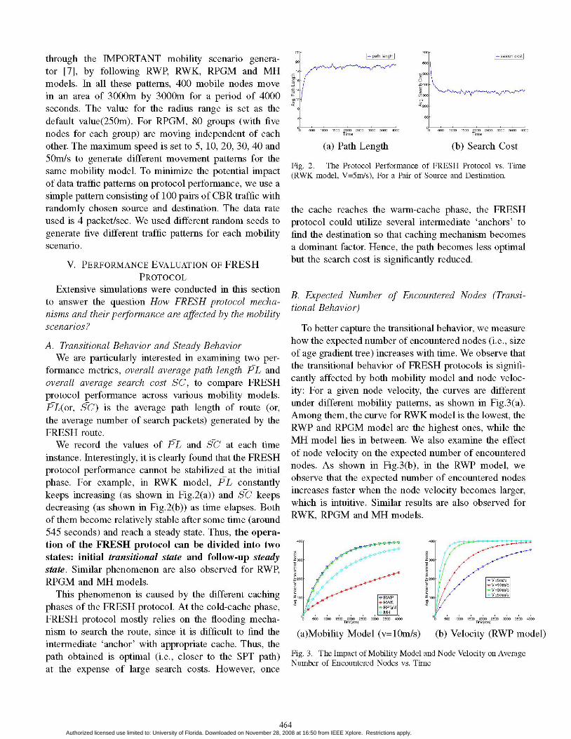
through the IMPORTANT mobility scenario genera-tor [7], by following RWP, RWK, RPGM and MHmodels. In all these patterns, 400 mobile nodes movein an area of 3000m by 3000m for a period of 4000seconds. The value for the radius range is set as thedefault value(250m). For RPGM, 80 groups (with fivenodes for each group) are moving independent of eachother. The maximum speed is set to 5, 10, 20, 30, 40 and5Om/s to generate different movement patterns for thesame mobility model. To minimize the potential impactof data traffic patterns on protocol performance, we use asimple pattern consisting of 100 pairs of CBR traffic withrandomly chosen source and destination. The data rateused is 4 packet/sec. We used different random seeds togenerate five different traffic patterns for each mobilityscenario.

V. PERFORMANCE EVALUATION OF FRESHPROTOCOL

Extensive simulations were conducted in this sectionto answer the question How FRESH protocol mecha-nisms and their performance are affected by the mobilityscenarios?

A. Transitional Behavior and Steady BehaviorWe are particularly interested in examining two per-

formance metrics, overall average path length PL andoverall average search cost SC, to compare FRESHprotocol performance across various mobility models.PL(or, SC) is the average path length of route (or,the average number of search packets) generated by theFRESH route.We record the values of PL and SC at each time

instance. Interestingly, it is clearly found that the FRESHprotocol performance cannot be stabilized at the initialphase. For example, in RWK model, PL constantlykeeps increasing (as shown in Fig.2(a)) and SC keepsdecreasing (as shown in Fig.2(b)) as time elapses. Bothof them become relatively stable after some time (around545 seconds) and reach a steady state. Thus, the opera-tion of the FRESH protocol can be divided into twostates: initial transitional state and follow-up steadystate. Similar phenomenon are also observed for RWP,RPGM and MH models.

This phenomenon is caused by the different cachingphases of the FRESH protocol. At the cold-cache phase,FRESH protocol mostly relies on the flooding mecha-nism to search the route, since it is difficult to find theintermediate 'anchor' with appropriate cache. Thus, thepath obtained is optimal (i.e., closer to the SPT path)at the expense of large search costs. However, once

-path length |~r

18-

, 16-

F- 14-

10

700-

600 )

-}5 500-

00

= 400-

U100-

60 500 1000 1500 2000 2500 3000 3500 4000

Time

(a) Path Length

0 500 1000 1500 2000 2500 3000 3500 4000Time

(b) Search Cost

Fig. 2. The Protocol Performance of FRESH Protocol vs. Time(RWK model, V=5m/s), For a Pair of Source and Destination.

the cache reaches the warm-cache phase, the FRESHprotocol could utilize several intermediate 'anchors' tofind the destination so that caching mechanism becomesa dominant factor. Hence, the path becomes less optimalbut the search cost is significantly reduced.

B. Expected Number of Encountered Nodes (Transi-tional Behavior)

To better capture the transitional behavior, we measurehow the expected number of encountered nodes (i.e., sizeof age gradient tree) increases with time. We observe thatthe transitional behavior of FRESH protocols is signifi-cantly affected by both mobility model and node veloc-ity: For a given node velocity, the curves are differentunder different mobility patterns, as shown in Fig.3(a).Among them, the curve for RWK model is the lowest, theRWP and RPGM model are the highest ones, while theMH model lies in between. We also examine the effectof node velocity on the expected number of encounterednodes. As shown in Fig.3(b), in the RWP model, weobserve that the expected number of encountered nodesincreases faster when the node velocity becomes larger,which is intuitive. Similar results are also observed forRWK, RPGM and MH models.

V 5m=sV=lOm/sV=30m/sV=50m/sRWP

RWKRPGMMH

ovi .~L~0500 1000 1500 2000 2500 3000 3500 4000

Time(sec)

(a)Mobility Model (v=10m/s)

6-0 500 1000 1500 2000 2500 3000 3500 4000

Time(sec)

(b) Velocity (RWP model)

Fig. 3. The Impact of Mobility Model and Node Velocity on AverageNumber of Encountered Nodes vs. Time

464

search cos.t|

400 F 400 F

z~300 z~3000

,=200~ ,, 2000

z 100 z 1000


C. Expected Path Length and Expected Search Cost(Steady Behavior)

We also examine the detailed steady behavior, i.e.,expected path length PL(Xn) and expected search costSC(xn) in FRESH for the destination with given SPTdistance (n hops away from the source)3. Fig.4(a) andFig.4(b) illustrate PL(Xn) and SC(xn), under variousmobility models at a given node velocity. The x-axis inboth figures is the SPT hop distance between a sourceand a destination, and the y-axis is the expected pathlength PL(Xn) or expected search cost SC(xn) for thepath with the given SPT distance, respectively. As shownin Fig.4(a), for a given SPT hop distance, the pathlength PL(xtn) for the MH model is the highest andthe RWK model has the lowest value, while the valuesfor RWP and RPGM models are nearly same and lie inbetween. As shown in Fig.4(b), SC(xn) increases withthe SPT hop distance n for all the mobility patterns. Fora given SPT hop distance, the RWP model generates thelowest overhead, and the other three mobility modelsare crossing over each other. When the hop distance nis small, the MH model incurs a larger search cost thanthe RWK and RPGM model.

4000v-RWPE RWK

13000 M

2000-

1000--v RWPRWKRPGMMH

10 15 20 25 30SPT Distance(hop)

(a) Path Length

10 15 20 25SPT Distance(hop)

(b) Search Cost

Fig. 4. The Expected Path Length and Expected Search Costobtained by FRESH protocol for all the Mobility Models (v=lOm/s)

We also examine the effect of node velocity on thesteady behavior of FRESH protocol for a given mobilitymodel. We observed that the steady behavior of theFRESH protocol is insensitive to the node velocity fora given mobility pattern. Both PL(Xn) and SC(xn) forRWP model are illustrated in the Fig.5(a) and Fig.5(b).Obviously, the different node velocity settings barelyhave an effect on the steady behavior of the FRESHprotocol. Similar results are also observed for RWK,RPGM and MH models.

Intuitively, FRESH protocols are supposed to behighly sensitive to node mobility at both transitionalstate and steady state. However, partly contrary to ourexpectation, we find out that the FRESH protocolperformance at transitional state is indeed sensitiveto both mobility model and node velocity setting,while its steady state behavior is only sensitive tounderlying mobility model but robust to node ve-locity. This further confirms the previous observationthat the FRESH protocol behaves differently under RWPand RWK model [4], by using an even richer set ofmobility models. Also, we shed some light on how thenode velocity affects the FRESH protocol, which is anew addition to previous observation. In this paper, it isthese observations that motivate us to develop the set ofanalytical models presented in Section VI and SectionVII, in an attempt to explore the reasons behind them.

VI. ANALYTICAL MODEL FOR NODE ENCOUNTERSAND WARM-UP TIME

We believe that the number of encountered nodesEi(t) is an important indicator to capture the cachewarm-up process. Thus, we are particularly interested indeveloping analytical model to identify the relationshipbetween the number of node encounters and its variousimpacting factors.

1500 V 5ms

co1000 V=0/3~50 V3-

V5500V=50m/s


(a) Path Length


(b) Search Cost

Fig. 5. The Steady-State Protocol Performance under RWP Model,for Different Node Velocities.

3The SPT distance between node A and node B, is the number ofhops from node A to node B along the Shortest Path Tree rooted atnode A.

A. Terminology

We first define the terms in our analysis as follows.1) N: The number of mobile nodes in the network.2) A: The width of the square-shape network field.3) t: The time elapsed since the system starts, 0 <

t < T, where T is the overall system operationaltime.

4) R: The communication range of wireless node.5) v: The average node velocity of mobile nodes.6) Ei(t): The expected number of encountered nodes

for node i at time t, i.e., number of created (notupdated) encounter table entries.

7) p: The effective average node density in the field.

465

55~

50

5000 F

~40

<] 30-

620-

10

30

40r 2000r

-300

1 200

100~

{iINCO Cb -


8) pi (t): The probability for node i that a nodeencountered at time t is really a node that nodei never encountered in the history.

Note that if the mobile nodes are uniformly distributedover the simulation field, then, the node density is pAN. In general, this is not valid for various mobilitymodels and node distributions. Hence, in general, weassume that the node density is p = 6 N, where 6 isthe constant compensation factor for the non-uniformlyfashion of node distribution(e.g., in MH model, wherethe nodes are only distributed along the freeway lanes,rather than uniformly distributed in the whole field).Different mobility models have different 6 values.

Also, for random mobility model, for node i, theprobability of encountering a new node (not encountered

befre)is ~(t N Ei(t)_ubefore) is pi(t) N. But, in general, to consider

all the mobility models, we assume that the probability ofbeing the freshly encountered node is pi (t) =1 NE(t)where t, is the constant compensation factor for the non-uniform node encounter probability distribution(e.g., inRWK model, the newly encountered node is more likelyto be a previously encountered node in contrast to RWPmodel, because the nodes in RWK model tend to wanderin its own neighborhood due to the strong temporalcorrelation). Different mobility patterns have different t,values.

B. Expected Number of Encountered Nodes

First, let us examine the number of nodes that node iencountered during the time slot At (after time t), i.e.,Ei(Atlt). During that time slot, the node i will travel inthe distance vAt, and the area covered by the wirelesstransmitter of node i is vAt x 2R = 2RvAt (Pleasenote the "incremental" area covered during time intervalAt (after time t) is not 2RvAt + wFR2, since the areawrR2 had already been covered at time t). Because thenode density in the field is p, the number of nodes thatnode i encountered during time slot At is 2RvAt x p.Within these encountered nodes, some are the nodes thatnode i has never encountered in the past, while othersare not. Thus, the number of 'freshly' encountered nodesfor node i during time slot At (after time t) is

Ei(Atlt) vAt x 2R x p x pi(t)

6r(2vRAt) NNE(t)

The number of encountered nodes at time t + At issum of the number of encountered node at time t andthe number of 'freshly' encountered nodes in the timeslot At. Hence,

Ei(t + At) Ei(t) + Ei(At t) (3)(1-0 A2vR 2vRN(1 A2At)Ej(t) + 6r At

Let c= 2nR1 = 2vfRN and Athe above equation, we have

Ei (t + At) -Ei (t) _ dEj (t) _At dt

:. Then, by using

-AaEi (t) + AO (4)

Eqn.4 is a standard differential equation about theunknown function Ei(t). Its general solution is givenby

Ei(t)p +ce-Aata

Nc 2vRAN + ce A2t (5)

where c is a constant factor to be determined.When t = 0, the nodes are static, and the encoun-

tered nodes are those within the radius range. Thus,the initial(boundary) condition is E (0) = AwN(N R)2Therefore, the constant factor c= (Aw (R) 2 1)N, andthe number of encountered nodes over time is

Ei(t) = N -N(1- AwF(j)2)e-A2AH (6)

When the simulation time is long enough (i.e., ap-proaches to infinity), the expected number of encoun-tered node is Ei(t - ox) = N. At that time, any specificnode has already encountered all the others.

Since the A values in Eqn.6 are too complex to be ana-lytically derived for various mobility models, we directlyestimate this value from simulation via the maximumlikelihood test, for different mobility models with thesame given velocity (v = 20m/s). We observe that the Aparameter is different for various mobility patterns. TheA parameter for RWP, RWK, RPGM and MH modelsare 1.92325, 0.71454, 1.8324 and 0.94365, respectively(when v = 20m/s). We then applied the curving fittingscheme to compare the experiment results collected fromsimulations and the analytical results based on Eqn.6 byusing this set of A values, for different mobility modelswith all the velocity settings (except v = 20m/s). Wecompare the error margin ratio between the simulationresults and results obtained from the analytical model.We find that the error margin ratio appears to be verysmall(< 2% in most cases), across all the mobilitymodels and all the velocity settings.


C. Warm-up Time

The warm-up time twarmup is defined as the time whenthe node encounter ratio exceeds a portion (i.e., y)4 ofall the other nodes. Hence, from Eqn.6, we are able toestimate the system warm-up time as

[ t > ~~~I ( (1--y

A))twarmup - ( _ 2v (7)A2vR-A A2

From Eqn.7, we can see that the warm-up time isa function of several key system parameters: the nodevelocity v, radius range R, and constant compensationfactor A which is unique for each mobility model.

VII. ANALYTICAL MODELS FOR EXPECTED PATHLENGTH AND EXPECTED SEARCH COST

At the warm-cache phase, we are particularly inter-ested in expected path length PL(xm) and expectedsearch cost SC(xm). We identify that these two per-formance metrics of FRESH protocol are directly deter-mined by the characteristics of age gradient tree.

A. Terminology

We first introduce the terms used in this section.1) Xm, x,n: The node Xnm(Xn) is the anchor node with

m-hops (n-hops) SPT distance from the destina-tion. For each search step in the FRESH operation,the upstream anchor xm discovers its downstreamanchor Xn along the age gradient tree (Vn, Vm, 0 <m, n < D). Please note m is not always greaterthan n in the FRESH protocol, even though xm isthe upstream anchor.

2) P(Xm, xn): The probability that upstream anchorXm discovers downstream anchor xn.

3) d(xm, xn): The average distance from upstreamanchor xm to downstream anchor xn, in terms ofhop counts.

4) C(Xmn, xn): The average search cost from upstreamanchor xm to its downstream anchor xn, in termsof transmitted packets.

5) PL(xm): The expected path length from anchorx,m to the destination via the path computed bythe FRESH protocol, in terms of hop count.

6) SC(xm): The expected search cost from anchorx,m to the destination, generated by the FRESHprotocol, in terms of transmitted packets.

4In our study, we define -y as 30%. As observed through simula-tions, both the characteristics of age gradient tree and the FRESHprotocol performance become stable after E(t) is larger than 30% oftotal node numbers.

7) /In,m The ratio of the path length for x,, to thepath length for xm, in the FRESH protocols, wheren > m. In other words, /tn,m PL(x,.") (wherePL(x,,)'n > m).

8) vnT,m: The ratio of the search cost for xn to thesearch cost for xm, in the FRESH protocols, wheren > m. In other words, Urn,m = SC(x-) (whereSC(x,,)'n > m).

Here, note that the parameters p(Qrm, Xn), d(xm, xn)and c(Xm, xn) are the characteristics of the age gradienttree representing the probability, the expected distanceand the expected cost from the upstream anchor to thedownstream anchor, respectively.B. Expected Path Length and Expected Search Cost

In the FRESH protocol, each upstream anchor x,m isin charge of searching its downstream anchor xn alongthe age gradient tree. The average distance from theupstream anchor xTm to the downstream anchor xn isd(xmT, xn). Considering the expected path length for theanchor xn is given as PL(xn), then, the path length fromanchor xTm to the destination via anchor xn is calculatedas PL(Xn) + d(xmT, xn). Also, the probability that up-stream anchor x,m discovers its downstream anchor xnis given as P(Xm Sxn). Hence,

D

PL(x,m) S x,(d(m x,2) + PL(xn,))p(xm, x,2)n=lmI1

(d(xm, X,n) + PL(xn))P(Xm, X,n)n=l

(1)

+ (d(xm, xm) + PL(xm))p(xm, xm)(2)

D

+ (d(xm, x,n) + PL(xn))p(Xm, x,n)n=m+I

(3)

(8)

(9)

where D is network diameter. Here, part(l), part(2)and part(3) corresponds to the cases in which the SPTdistance from upstream anchor to the destination (mhops) is larger than, equal to, or smaller than the SPTdistance from the downstream anchor to the destination(n hops), respectively. The equation could be solved ina recursive manner. For the upstream anchor xm with agiven hop distance m, the path length for the downstreamanchor PL(xn) (Vn, n < m) in part(l) is already known.For the case where n > m (in part (3)), by substitutingPL(xn) = tn,mPL(xm)(where n > m) into part(3) of


Eqn.9 and then simplifying Eqn.9, we get the expected After replacing the n factor and v factor bypath length for anchor x,m along the path obtained by Eqn.12 and Eqn.13, we get the analytical models for theFRESH protocol as expected path length and the expected search cost in

the FRESH protocol (in recursive format) asPLf ) ," 1d(x,,,x,)p(x,,,x,)+E_' PL(x,)p(x,,,,t)PL(x,) En1 pn=1~)ZLX;m 1~~-p(Xm 'X")-Yn=m+l 11tn,mP(X,,Xn)

(1

Similarly, we get the expected search cost as

SC(m) 1 ~(XTmXn)P(XTXn)+ET SC(Xn)p(XT,Xn)SC(XT1) =-xn1 D

n=1

1-P(XTmXT')-En=m+l Vn,mP(X,,,Xn)

(1

However, the parameters PnU,m in Eqn.10 and vn,, inEqn. 11 remain unknown. Through our derivations, wefind that the path length of FRESH paths is linearlycorrelated with its SPT path length. Hence, the parameter/Atn,m is

PL(4FRESH) n/lr,m = PL(XFRESH) at (12)

Also, we find that search cost of FRESH path ispolynomially correlated with its SPT path length. To bein details, the parameter vn,m is also a function of theirSPT distances, as

SC( RESH) 2n311i,m -SC(XFRESH) 2m3

3n2 + n

.3m2 + m

We also validate both Eqn.12 and Eqn.13 by takingthe measurement of the path length ratio /I ,m and searchcost ratio v,,m (where n > m) in the FRESH protocol,through simulations. The results indicate that, in mostcases, Eqn.12 and Eqn.13 are reasonable approximations

.5of real scenarios

5We acknowledge that the both equations (Eqn. 12 and Eqn. 13)are only the approximations of the realistic scenarios. However, theaccuracy of the analytical models (Eqn.10 and Eqn. 1) will not besignificantly affected. This is because, intuitively, we know that itis a rare case that an upstream anchor will search a downstreamanchor whose SPT distance to destination is even much larger thanits own SPT distance to the destination. Through the simulation,we observe that P(Xm,Xn) is a very small value if m < n <m + E, and P(Xm,Xn) = 0 if n > m + E (in most mobilityscenarios, K< 2). At the same time, the value P(Xm, xn) (wheren < m) seems to be a very large value compare to the valueP(xm, x,) if n > m. That is to say, even the approximation ofun.m and v'n,m is not exactly accurate, the small values of p(Xm, x )(n > m) enables the item En=m+l/1 n,mP(Xm, Xn) (in Eqn.10) and

>ZD m+1 Pn,mpQm, Xn) (in Eqn.11) to be very small values. Thus,the accuracy of the estimation based on Eqn. 15 and Eqn. 16 will notbe affected significantly by these approximations made in Eqn. 12and Eqn. 13. We further validate our argument through extensivesimulations.

0PL(xm )

SC(X,m)

1)

1d(xm ,x)p(xm ZUx)+n1 PL(xt,)p(xmxn)1-n=l n=l-E+ mpt 7n

withPL(xi) = 1 (14)

Zuii 1(m(XT X)P(XT ,Xn )+Y: SC(Xn)P(XT,,X,,)1-p(xxm)-~ 1nm+l 2m3-3m2+mP( )

withSC(xl) = 1 15)

As shown in Eqn.14, for a given m value, the expectedpath length PL(xm) is a function of the characteristicsof age gradient tree (d(xm, x,2), P((xm:, x,)) and theexpected path length of the paths whose SPT distancesmaller than m hops (PL(x,2), where 1 < n < m).Similarly, as shown in Eqn. 15, the expected search costSC(xm) is also a function of the characteristics of agegradient tree (C(Xm, Xn), P(Xm, xn)) and the expectedsearch cost of the paths whose SPT distance is smallerthan m hops (SC(xn), where 1 < n < m).

Both Eqn.14 and Eqn.15 should be solved in a recur-sive fashion, from smallest m value(m = 1) to the largestm value (m = D). Intuitively, the initial conditions forrecursive-format Eqn.14 and Eqn.15 are PL(xi) = 1 andSC(xi) = 1. Starting from these initial conditions, weare able to estimate the expected path length PL(xm)and expected search cost SC(xm) based on these twoanalytical models, if the characteristics of age gradienttree (d(xm, x,n), C(Xm, x,n) and P(Xxm, xn)) are given.

Again, we compute the error margin ratio between thecalculated result (based on Eqn.14 and Eqn.15) and themeasured result (from simulation). Through the study,we find the error margin ratio for the expected pathlength is 5% -10% and the error margin ratio for theexpected search cost is around 6% -17% in all themobility scenarios. The acceptable error margin ratiosindicates that the proposed analytical models are goodapproximations to study the steady behavior of FRESHprotocol based on the measurement of the character-istics of age gradient tree (d(xm,xn), C(Xmnxn) andP(XmT, xn))-

VIII. THE LOGICAL RELATIONSHIP BETWEENMOBILITY, AGE GRADIENT TREE AND FRESH

PROTOCOL

Finally, we attempt to answer questions Why FRESHprotocol is, or, is not, affected by the underlying mobility


scenarios?, by developing a logical relationship amongall the components.

A. Temporal-Spatio Correlation and Age Gradient Tree

Temporal-spatio correlation, which exists for all themobility models discussed in this paper, can be used toroughly estimate the distance between nodes, based ontheir last encounter time. However, note that differentmobility models exhibit different types of temporal-spatio correlation. To vividly illustrate the temporal-spatio correlation, we examine the 3-D age gradientfield. For a specific destination, the age gradient fieldis formed if each node on the 2-D space is associatedwith its encounter age for the destination (as its z-axis),which represents the 'potential' (similar to the meaningof 'potential' in physics). As shown in Fig.6(a) andFig.6(b), the age gradient fields for RWK model andMH model are like funnels (whose sink is the givendestination), indicating the spatial distance between anode and a destination is somehow correlated with theirencounter age. Similar temporal-spatio correlation is alsoclearly observed for RWP and RPGM models.

(b)RWPI -1

(c)MH (d)RPGM

Fig. 7. The Age Gradient Tree (AGT) for RWP, RWK, MH andRPGM models (v=20m/s, t=400sec). Here, D is the destination, andalso, the root of AGT.

2000 1000

3000 0X(m) Y (m)

Fig. 8. The Temporal-Spatio Correlation of a given destination nearcenter, for the RWK model (V=50m/s), measured from simulation.

in Section III-B). Therefore, age gradient tree is an'

abstracted form of the temporal-spatio correlation.a)

a) 400-

' 200-8

3000 o.-0

2000

Y (m)

(a)

-2000-- ~000

0 0 X(m)

RWK model

2000 ,1_000-loo3000 o

X (m) Y (m)

(b) MH model

Fig. 6. The Temporal-Spatio Correlation of a given destination forthe RWK and MH model (V=30m/s), measured from simulation. Wepick one node close to the center of simulation field as the destination,for better illustration.

The age gradient field implicitly designates the routefrom any node to the given destination. In other words,because of this temporal-spatio correlation, the packetsare able to gradually move from upstream anchor to-wards downstream anchor and finally reach the destina-tion. Hence, we believe that temporal-spatio correla-tion is the key reason enabling the mobility-assistedencounter-based FRESH protocol. FRESH protocolwill not function well if this temporal-spatio correlationdoes not exist.

Rather than being used directly, the 3-D temporal-spatio correlation and the designated routes on the funnelsurface are projected onto the 2-D space, forming anage gradient tree (exactly the same 'age gradient tree'

B. The Impact of Mobility on Age Gradient Tree andFRESH Protocol Performance

Through Section V, we know that the performanceof FRESH protocol at steady state is fully determinedby characteristics of age gradient tree. Here, we mainlyfocus on the impact of mobility on the behavior of agegradient tree at steady state, i.e., how the shape andthe characteristics of age gradient tree behave underdifferent mobility models and node velocities. First,we discuss the case of different mobility models withsame velocity. Intuitively, different mobility models cre-ate different encounter patterns and hence the differenttypes of temporal-spatio correlation, as shown in Fig.6(a)(RWK) and Fig.6(b) (MH). Also, as shown in Fig.7,the shape of age gradient tree for RWK, RWP, RPGMand MH mobility models are visually different (andso are their characteristics). For example, in the MHmodel, the age gradient tree consists of age gradientson the horizontal and vertical lines because nodes arerestricted to the Manhattan map (as shown in Fig.7(c)).Next, we examine the case of same mobility model withdifferent velocities. Here, interestingly, we observe thatthe shapes and characteristics of age gradient tree for the

469

600-0a)Aa) 400, 140)

'E. 200-D00C:LU

0-0 -------------...ooo:..

2000

"I .I.x

600 rI'l

,3- 800-a)

.' 600ol

400-2. 200-0

w 0 '

3000 -

30001 000


same mobility model are similar under the different nodevelocities. Quantitatively, for a given mobility model,the error margin ratio for p(rm, x2n), d(xmn,xn) andC(X,m, xn) between different velocities is very small (lessthan 5.25%, 4.06% and 8.45%, for all these four mobilitymodels). To sum up, for steady state, we observe thatthe mobility model significantly affects the shape andthe characteristics of the age gradient tree, while thevelocity settings may not.

This counter-intuitive observation can be explainedin this way: With the different node velocity settings,the exact encounter age between nodes may differ andthe height of 3-D temporal-spatio correlation may bedifferent (e.g., the height of funnel is around 800 secin Fig.6(a), while the height is about 400 sec in Fig.8).However, its rough shape and the designated routes onthe funnel surface (the age gradient from the node withlarger encounter age to the node with smaller encounterage) do not change drastically, as shown in Fig.6(a)(v = 30m/s) and Fig.8 (v = 50m/s). In other words,once the 3-D temporal-spatio correlation is projected tothe 2-D field, the information of exact encounter age(z-axis value) becomes useless. In this way, the nodevelocity only contributes to 'scale' the encounter age butdoes not affect their relative relationship which forms theage gradient tree. Hence, the shapes (and characteristics)of age gradient tree under different node velocity arenearly same for a given mobility model.

Therefore, the FRESH protocol, whose performance isdetermined by the characteristics of the age gradient tree,behaves differently for various mobility models but lesssensitive to different node velocities. We, thus, believethat the characteristics of age gradient tree are thekey bridge linking the mobility effect and the protocolbehavior of FRESH protocol6.

IX. CONCLUSION & FUTURE WORK

In this paper, we quantitatively analyze the com-plicated interaction between the mobility and the lastencounter based protocol (i.e., FRESH) which directlyutilize mobility information to discover node location orroute. First, we evaluated the FRESH protocol over a richset of mobility models by which we believe that mobilityspace could be spanned. We found that the transitionalbehavior of FRESH protocol is significantly affected by

6The role of age gradient tree in FRESH protocol is same to that ofLink Duration and Path Duration in the SPT-based MANET routingprotocols [9]. We believe that, because of the different protocol mech-anisms, it is necessary to examine the different connectivity graphproperties which are directly relevant to the protocol mechanism.

underlying mobility scenarios, while its steady behavioris less sensitive to the node mobility. Motivated bythese observations, we developed a set of analyticalmodels to capture the FRESH protocol behavior at bothtransitional state and steady state, and we also realizethat age gradient tree is the key to explain the complexinterplay between node mobility and last encounter basedprotocol.

The analytical models and qualitative analysis notonly deepen our theoretical understanding itself, butalso contribute to practical protocol design enhancement.Partly inspired by the fact that the age gradient tree isinsensitive to the node velocity, we also aim to design amore practical protocol whose performance is robust tonode velocity(based on Eqn.15 and Eqn.16). Throughour study, we feel that AGT-based mobility-assistedprotocols hold great potentials for the future wirelessnetwork, and this topic deserves more attention fromresearch society.

REFERENCES

[1] K. Fall. "A delay-tolerant network architecture for chal-lenged intemets", In Proceeding of ACM SIGCOMM, 2003.

[2] M. Grossglauser and D. Tse. "Mobility increases the capac-ity of ad-hoc wireless networks", In: Proceeding of IEEEINFOCOM 2001.

[3] T. Small and Z. Haas. "The Shared Wireless InfostationModel - A New Ad Hoc Networking Paradigm (or Wherethere is a Whale, there is a Way)". In Proceeding of ACMMobiHoc, June 2003.

[4] H. Dubois-Ferriere, M. Grossglauser, and M. Vetterli. "Agematters: Efficient route discovery in mobile ad hoc networksusing encounter ages", In Proceeding of ACM MobiHoc,June 2003.

[5] M. Grossglauser and M. Vetterli. "Locating nodes withEASE: Mobility diffusion of last encounters in ad hocnetworks", In Proceeding of IEEE INFOCOM, April 2003.

[6] J. Broch, D.A. Maltz, D.B. Johnson, Y-C. Hu, J. Jetcheva,"A performance comparison of multi-hop wireless ad hocnetwork routing protocols", in: Proceedings of ACM Mobi-com 1998, Roma, Italy.

[7] F. Bai, N. Sadagopan, A. Helmy, "IMPORTANT: a frame-work to systematically analyze the impact of mobility onperformance of routing protocols for ad hoc networks", inINFOCOM 2003.

[8] W. Zhao, M. Ammar and E. Zegura, "A Message FerryingApproach for Data Delivery in Sparse Mobile Ad HocNetworks". In Proceedings of ACM MobiHoc 2004, TokyoJapan.

[9] F. Bai, N. Sadagopan, B. Krishnamachari, A. Helmy, "Mod-eling Path Duration Distributions in MANETs and theirImpact on Routing Performance", IEEE Journal on SelectedAreas of Communications (JSAC), Vol. 22, No. 7, pp. 1357-1373, September 2004.


impact of mobility on last encounter routing protocolshelmy/papers/maid-secon... · this research...

Documents