impact of interest rate risks on life insurance assets and liabilities examensarbete 2006:19
TRANSCRIPT
Mathematical Statistics
Stockholm University
Impact of Interest Rate Risks on
Life Insurance Assets and Liabilities
Hao Wu
Examensarbete 2006:19
ISSN 0282-9169

Postal address:Mathematical StatisticsDept. of MathematicsStockholm UniversitySE-106 91 StockholmSweden
Internet:http://www.matematik.su.se/matstat

Mathematical StatisticsStockholm UniversityExamensarbete 2006:19,http://www.matematik.su.se/matstat
Impact of Interest Rate Risks on
Life Insurance Assets and Liabilities
Hao Wu∗
November 2006
Abstract
This paper examines the impact of interest rate risk that a lifeinsurer is subject to, especially the effect of interest rate risk on therestricted assets and the technical provisions. The main work has beenestimating the yield curves and scenario analyzing. Stress test hasbeen applied for this purpose, aiming to get a suitable match betweenthe assets and liabilities in such a way that changes in interest ratesby shifts do not affect the financing of liabilities.
Keywords : Extended Nelson-Siegel model, yield curve, technical
provisions, restricted assets, and traffic light system.
∗E-mail: [email protected]. Supervisor: Thomas Hoglund.

ACKNOWLEDGEMENTS
This report is a 20 credits thesis in mathematical statistics, mainly performed at TheSwedish Financial Supervisory Authority, Finansinspektionen.
First of all, I would like to express my sincere gratitude and appreciation to mysupervisors at Finansinspektionen, Jan Röman and Göran Ronge who have beensupportive to me since the moment I entered the Finansinspektionen. Their help andencouragement are important for me to carry out this thesis, and it has become a fullyenjoyable learning process to write the thesis. I would also like to acknowledge mysupervisor at mathematical statistical institution at Stockholm University Prof. ThomasHöglund for his professional advice and judgment.
I am grateful for the discussions with Björn Palmgren (Finansinspektionen), RikardBergström (PP Pension) and Tony Persson (Alecta), who inspired me with great ideas inboth life insurance mathematics and risk management.
I would also like to take this opportunity to thank faculty members of mathematicalstatistical institution at Stockholm University for guiding me through the ActuaryProgram.
I also give my special thanks to my family: mother Leizhen Zhang, father Shunchao Wu,brother Po Wu and my husband Hao Mo for their encouragement and support.

1
CONTENTS
1 Introduction -------------------------------------------------------------------------- 2
2 Fixed-income securities ---------------------------------------------------------- 42.1 Term structure of interest rate2.2 Risk measures for the term structures
3 Parametric model for the yield curves ----------------------------------------- 83.1 Nelson-Siegel Model3.2 Extended Nelson-Siegel Model
4 Estimation for the yield curves --------------------------------------------------- 124.1 Criterion for the estimation4.2 Data selection4.3 Estimates of parameters4.4 Impact of the yield curves4.5 Alternative yield curves
5 Parametric effects on the yield curve -------------------------------------------- 185.1 Influence of parameter _05.2 Influence of parameter _1 and 1τ5.3 Influence of parameter _2 and 1τ5.4 Influence of parameter _3 and 2τ
6 Life insurance mathematics -------------------------------------------------------- 236.1 Pension system in Sweden6.2 Life insurance risks6.3 Cash flows valuation
7 The problem of mismatch for a life insurer -------------------------------------- 277.1 Mismatch between the asset and liability7.2 The restricted assets7.3 Sensitivity to the interest rate risk
8 Conclusions ---------------------------------------------------------------------------- 34
9 References ----------------------------------------------------------------------------- 36
10 Appendix ------------------------------------------------------------------------------ 38

2
1 INTRODUCTION
On January 1, 2006 the Directive on Institutions for Occupational RetirementProvisions (IORP Directive) came into force in Sweden. This is the beginning of aseries of regulatory changes in the insurance area over the next few years. The TrafficLight System, as a new supervisory tool is designed by The Swedish FinancialSupervisory Authority (Finansinspektionen) aiming to measure financial risks (seefigure 1) that life insurance companies and occupational pension funds may be exposedto. Finansinspektionen believes the earlier identification of insurers with high financialrisk, the better protection can be achieved for the policyholders. The main risk thatundertakings are subject to is interest rate risk, with consideration to the fact thatinsurance liabilities often have long durations. In our study, the insurance businessconsists of occupational life long pensions on a defined benefit basis, occupationaltemporary pensions on a defined contribution basis and private pensions, temporaryand life long. Such a composition obviously generates a long duration of our liabilitiesthat are very sensitive to the changes in interest rates. So in this paper, the risk ofinterest rates stands in the focus.
Figure 1: Overview of financial risks
According to the Traffic Light System, life insurers are required to follow the PrudentPerson Principle in the case of valuing their technical provisions. Finansinspektionenemphasizes that each transaction in an insurance contract must essentially bediscounted individually using the risk free rate of interest that corresponds to theduration of the liabilities, provided that an institution can categorize its liabilities in thismanner. For an institution that cannot apply cash flow categorization, the problem canbe solved by other approximate measures, which we will not take into account in thiswork.
Total Risk
Fluctuations in a life insurance company value
Financial Risk Operational Risk Insurance risk
Int erest rate risk
Liquidity risk
Re al estate risk
Credit ris k
Exchange ri sk
Equ it y ri sk
Actuarial
assumptions made
in different lines of
insurance business

3
As we mentioned above, the cornerstone of the Prudent Person Principle is valuing thetechnical provisions at their realistic value. It gives rise to a series of changes in theannual report. First of all, as an opposite financial position in a balance sheet, therestricted assets have to respond to the changes in the technical provisions. In otherwords, this principle requires insurers to increase their restricted assets in bothquantities and qualities, so the assets at least will satisfy the solvency ratio requirement.Furthermore, from the view of risk taking a proper balance between the assets andliabilities is expected for a life insurer. In the following figure, we try to summarize thestructure of balance sheet affected by the Prudent Person Principle.
Figure 2: Overview of existing balance sheet in a life insurance company after introducing theTraffic Light System
Available solvency margin
Safety margin
Required solvency margin
Realistic value
Restricted assets Technical
provisions
Free assets
---------------------
Share capital and
other equity
--------------

4
2 FIXED-INCOME SECURITIES2.1 TERM STRUCTURE OF INTEREST RATE
Term structure theory puts aside the notion of yield, and instead focuses on therelationship between financial securities of different terms. The term structures ofinterest rates, also known as the yield curves therein interest rates are determined bytheir terms. The curves usually slope gradually upward as maturities increase. Suchtypical shape of yield curves reflects the expectation hypothesis in which market’sexpectation for the future interest rates is explained on the basis of the current marketconditions.
Government treasuries are considered risk free. Their yields are often observed asbenchmarks for the fixed-income securities with the same maturities. Here we givesome examples for the most popular financial securities, zero-coupon bonds andcoupon bonds.
• Zero coupon bondsA zero coupon bond is a debt security that does not pay coupons during its life, but it istraded at a deep discount to its face value, which will be worth when the bond maturesor comes due. Zero-coupon bonds have an important advantage of being free ofreinvestment risk, though such bonds cannot enjoy the effects of an interest rate rise.Zero coupon bonds tend to be very sensitive to the changes in interest rates. Theirprices fluctuate more than other types of bonds in the secondary market in the since thatthere are no coupons during their life to reduce the effect of the changes in interestrates.
• Coupon bondsA coupon bond is a debt obligation with coupons affixed to the bond itself, and eachcoupon represents a single interest payment.
The current price of a bond should be the same as the present value of the stream offuture cash flows, which is the nominal amount of money to change hands at somefuture date, discounted to account for the time value of money, e.g. interest rate.(http://en.wikipedia.org/wiki/Present_value). Present value of a stream of cash flowscan be obtained by adding discounted magnitudes of the individual cash flows due tothe present value is additive. It should be noted that sooner the money is received, morevalue it is worth if it is compared with the same amount of money that is received latersince interest can be earned by loaning money out.
Suppose there is a stream consisting of several payments at the end of each period fortotal of n periods ),...,,( 21 nXXX and m times per year. Interest rate r is the nominalannual compounded interest rate. In the formula below, PV is used to denote the presentvalue of the stream of payments (consisting of the coupon payments and the final face-value redemption payment).

5
In a context of finance, discounting is referred to a process of calculating the presentvalue of future monetary amounts. With the help of discount factor, a future cash flowcan be valuated at a given time that we are interested in. Let td indicate the discountfactor for its term t. The value of td can be obtained by the formulas below with theconsideration of different types of interest rates. Suppose that the fixed annual interestrate r compounded m times per year for total t periods, and then the appropriatediscount factor is
In the case of continuous compounding, we gave the following formula
2.2 RISK MEASURES FOR THE TERM STRUCTURES
We start this section with introducing a conception of yield. Yield for a bond isthe effective rate of interest paid on the bond, at which the present value for a stream ofpayments is exactly equal to the current price of the bond. The stream here consists ofall coupon payments and the final face-value redemption payment. This effective rateof interest is always quoted on an annual basis, and termed more properly as yield tomaturity (YTM).
Formulas below are given for the bond prices therein coupon payments made at the endof each period of total n periods, and m times per year. Time to maturity is T years,which equates with n/m. YTM is constant and denoted by λ, the payment that made inperiod k is indicated to kC , and its present value is denoted by kPV .
Duration is a measure of time until a bond gives a profit. It is useful in the sense that itdirectly measures the sensitivity of prices to the effects of changes in YTM. For a zero-coupon bond, duration is the same as its time to maturity. For a coupon bond, durationis strictly less than their life period. We start our discussion about this measure withintroducing two kinds of durations. Suppose we have coupon payment made m times
mkteXPV
mrXPV
k
n
k
n
kk
k
ktr
kt=⋅=
+=
⋅−∑
∑
=
=
here w gcompoundin Continuous
]1[ rateinterest Compound
0
0
mkteCPVPVP
m
CPVPVP
ktk
n
kk
k
kk
n
kk
ktk
===
+==
⋅−⋅
=
=
∑
∑
and where, price Bond : gcompoundin continuousWith
]1[ where, price Bond :rateinterest compoundWith
1
1
λ
λ
[ ]kmrdk
+=1
1
mkted k
ktrk ==
⋅− re whe

6
per year in T years, YTM is λ and kC is the payment that made in period k. Macaulayduration of such a bond can be found according to the following formula.
It is easy to realize that Macaulay duration is the average of the stream of paymentsover the life of a bond, each coupon payment is discounted on the basis of a commonyield curve. The other duration we want to mention here is Modified duration. Therelationship between these two durations can be described by the following.
It should be noted that for large values of m - the number of payments made per year orsmall values of YTM, we have Dmacaulay ≅ Dmodified. With the help of modified duration,derivation of bond price with respect to λ can be reduced to the following expression.
That can be even rewritten as following
(*)
With the help of the formula above, we readily realized that modified duration revealsthe relative slope of the price-yield curve at a given point. A certain percentage changeof bond price leads to a corresponding change of the yield curve. That gives a straight-line approximation to the price-yield curve.
Another risk measure for the sensitivity of price-yield curve is convexity, whichmeasures a certain percentage change in the modified duration if the yield increaseswith one basis point. Convexity is defined as below
If the bond price P is described in terms of cash flows, the formula above will have adifferent appearance. In the following formula, coupon payments are paid m times peryear for total n periods; kC is the payment that made at period k, and its present value isdenoted by kPV .
[ ]∑= +
⋅=n
k
kmacaulay k
m
Cmk
PD
1 )(1
1λ
m
DD macaulay
λ+
=1
modified
PDPD
m
n
kkPVP
×−≡××+
−=∑= ∂
∂=
∂∂
modifiedmacaulay1
1
1 λλλ
)2(modified λολ ∂+∂×−=∂ DPP
2
21Convexityλ∂∂
=P
P
[ ] [ ] 211
2
2 )1(
)(1)(1
11Convexity2 m
kk
m
C
mP
PVP
n
k
kn
k
kk
+⋅
++=
∂
∂= ∑∑
== λλλ

7
With the help of convexity, the formula (*) can be derived even further. A betterapproximation for the price-yield curve can be achieved by taking in the second-orderderivative.
As we mentioned earlier in this section, the current price of a bond is exactly equal tothe present value for the stream of its coupon payments. The way to calculate Macaulayduration and Modified duration for a single bond can be utilized to a portfolio as well.Suppose there is a portfolio, in which several bonds (say m) with different durations areassembled. Let Pi and Di denote the price and duration for these bonds respectively,and i= 1, 2 …m. The value of such portfolio can be obtained by the formula belowtherein P and D are used to denote the value of this portfolio and its duration,respectively.
[ ] [ ] )()1(
)(1)(1
1 322
1modified
2λολ
λλλ ∂+∂×
+⋅
+++∂×−=
∂∑= m
kk
m
C
mPD
PP n
k
k
k
,...m,iPPwDwDwDwD
PPPPi
imm
m
21 and where...
...
21
21
21 ==+++=
+++=
8
3 PARAMETRIC MODEL FOR THE YIELD CURVES
Estimates of the yield curves are required to have enough flexibility in order torepresent the shape associated with the curves, which means the estimates shouldprovide a maximal approximation to the observed data. God precision of the estimatesis another requirement with the consideration of the analytical demands in the contextof monetary policy.
In 1987, Nelson, C.R. and Siegel, A.F. published their parsimonious modeling of yieldcurves (so-called Nelson-Siegel Model), which successfully seized a trade-off betweenthe smoothness of the estimated curve and the flexibility. In 1994, Svensson, L.E.Oextended Nelson-Siegel Model by his work ‘Estimating and interpreting forwardinterest rates’ (so-called Extended Nelson-Siegel Model), in which he demonstrated theuse of forward interest rates as a monetary policy indicator. He also pointed out ‘theforward rate curve more easily allows a separation of expectations for the short,medium and long term than does the yield curve’.
Litterman and Scheinkman in 1991 claimed that most of the observed variation in bondreturns could be explained by three factors baptized to the name – level, slope andcurvature. Their findings provided another interpretation of short-, medium- and long-term components for the estimates of the yield curves, which were used in the paperwritten by Nelson and Siegel.
According to BIS (Bank for International Settlements), most central banks haveadopted either Nelson-Siegel or Extended Nelson-Siegel Model, except those countriesCanada, Japan, the U.K and the U.S. In the case of Sweden, Riksbank - Sweden’scentral bank adopted the ‘smoothing splines’ method in 2001, but it still reportsExtended Nelson-Siegel estimates to the BIS Data Bank.
3.1 NELSON-SIEGEL MODEL
This model is motivated by, but not dependent on, the expectation theory of the termstructure. It offers a parsimonious representation of the range of shapes associated withthe term structure of interest rate: monotonic, humped and S shaped. The model hasadvantages of estimating lesser number of parameters and therefore ensuring a smoothforward curve.
In order to understand the ideas of Nelson-Siegel model, we start our discussion aboutthis model with recalling the definition of instantaneous forward rate and finite-maturity forward rate. Suppose that mts , is the spot interest rate for a zero coupon bondtraded at a given point of time t and matures at time m; ),,( mitf is the forward ratewith trade date t, settlement date i and maturity date m. Below we gave the formulasthat describe the relationship amongst spot interest rate, instantaneous forward rate (theforward rate for a forward contract with an infinitesimal investment period after the

9
settlement date) and finite maturity forward rate. It should be noted that the possiblevalue of m must be higher or equal to the value of i.
Nelson-Siegel Model derives the instantaneous forward rate ),,( tmf Θ at maturity m ina functional form given below where Θ denotes the parameters β0, β1, β2, τ1 that needto be estimated from the observed data, and t indexes to the point of time at whichestimation is carried out.
This forward rate model generates a family of forward rate curves that take onmonotonic, humped, or S shapes depending on the values of beta-parameters. Nelsonand Siegel interpreted the coefficients of each component as indicators that measure thestrengths of the long-, short-, and medium-term components for the forward rate curve.The long-term component is constant that does not decay to zero in the limit. The short-term has the fastest decay of all functions that decay monotonically to zero. Themedium-term starts out at zero and decays to zero. Figure 3.1 shows the characteristicsof these components for the forward rate curve. There the contribution of the long-termcomponent β0 is equal to 1.
Figure 3.1: Components of forward rate curve estimated by Nelson-Siegel Model
Based on the forward rate model, the yield for zero-coupon bonds with differentmaturities is denoted as ),,( tmR Θ , which can be obtained by integrating the forwardrate function from zero to m and then divided by m. ),,( tmR Θ is actually the average offorward rates over time.
0
0,2
0,4
0,6
0,8
1
1,2
0 2 4 6 8 10 12 14
time to maturity
mod
el v
alue
s
long term short term exp(-m) medium term m*exp(-m)
( )
( )tm
m
tuduutf
mitfim
im
m
iuduutfim
iits
mmts
mtsitf
mitfmitf
−
∫==
→=
−
∫==−
−
+
+=
),( ,,lim
),(
1)(
1
),1(
,1
,),(
),,(),,(
−⋅⋅+−⋅+=Θ )exp()exp(),,(,1,1
,2,1
,1,0tt
tt
ttmmmtmf ττ
βτββ

10
We realize that the value of ),,( tmR Θ converges to β0,t as maturity goes to infinity.That is the reason that β0,t is interpreted as contribution of the long-term component ofthe curve. It indicates the level of the term structure of interest rates. The estimatedvalue of β0,t should be obviously positive.
),,( tmR Θ converges to β0,t+ β1,t as soon as m decreases to zero. To understand this, itis better to go back to the forward rate model therein β1,t is the coefficient of a termdecaying monotonically and fast to zero. β1,t determines the starting value of the curvein terms of deviation from the asymptote β0,t, and this is why Nelson and Siegelconsidered this parameter as contribution for the short-term component. β1,t indicatesthe slope of the yield curve.
In the yield function ),,( tmR Θ , the coefficient of the third component - β2,t specifiescurvature of the yield curves. As long as the sign of β2,t is determined, hump (positive)or U shape (negative) is made. The absolute value of β2,t indicates the magnitude of thecurvature.
In the case of parameter τ1,t, it should be positive and determines the position of thecurvature for the estimated yield curve.
3.2 EXTENDED NELSON-SIEGEL MODEL
Svensson L.E.O. extended the Nelson-Siegel model by an additional component inwhich two parameters β3,t and τ2,t were involved. In other word, Extended Nelson-Siegelmodel consists of total six parameters β0,t, β1,t, β2,t, β3,t, τ1,t and τ2,t. The forth componentcreates an additional turning point in the estimated curve. In the context ofparsimonious modeling of the yield curves, Nelson-Siegel model is usually consideredas a restrictive application for the Extended Nelson-Siegel model. The yield function isgiven below
The additional parameter τ2,t should be greater than zero, and indicates the position ofthe second hump or the U-shape on the curve. Parameter β3,t has the same function asparameter β2,t , its sign determines the shape of the estimated curve and its absolutevalue indicates the magnitudes of the second curvature.
−−
−−⋅+
−−⋅+=Θ )exp(
)exp(1)exp(1),,(
,1,1
,1,2
,1
,1,1,0
tt
tt
t
ttt
mm
m
m
mtmR τ
τ
τβ
τ
τββ
−−
−−⋅+
−−
−−⋅+
−−⋅+=Θ )exp(
)exp(1)exp(
)exp(1)exp(1),,(
,2,2
,2,3
,1,1
,1,2
,1
,1,1,0
tt
tt
tt
tt
t
ttt
mm
mm
m
m
m
mtmR τ
τ
τβτ
τ
τβ
τ
τββ
11
Figure 3.2 below shows the characteristics of these four components in Extended N-Smodel. Total sex parameters are estimated from the data set selected on 28, April2006, and their estimated value are β0,t = 3,40%, β1,t = -1,37%, β2,t = -2,03%, τ1,t =0,43, τ2,t = 5,57 and β3,t = 1,97%.
Figure 3.2: Components of the yield curve estimated by Extended N-S model.
-10,00%
-8,00%
-6,00%
-4,00%
-2,00%
0,00%
2,00%
4,00%
6,00%
1 9 17 25 33 41 49 57 65 73 81 89
time to marturity
valu
e
the first component the second component the third component the forth component
12
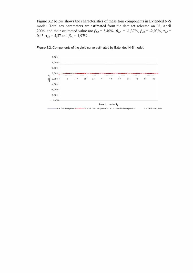
4 ESTIMATION FOR THE YIELD CURVES4.1 CRITERION FOR THE ESTIMATION
Parameters in Nelson-Siegel or Extended Nelson-Siegel model can be estimated byminimizing either the sum of squared bond-price errors or the sum of squared yielderrors. Decision of whether the first or the later should be applied depends on thepurpose of estimation.
However, as pointed out by Svensson (1994) minimizing price errors sometimes resultsin fairly large yield errors for bonds with short maturities. This is because prices arevery insensitive to yields for short maturities. BIS (Bank for International Settlements)also noted that using bond prices in the estimation irrespective to their durations wouldlead to over-fitting of the long-term bond prices at the expense of the short-term prices.Facing this problem, several approaches have been introduced amongst which the mostpopular remedy is non-linear least squares algorithm e.g. the price error of each bond isweighted by the inverse of its duration, so-called interest rate sensitivity factors ofprice.
In the formula below, y indicates the yield, jP is the market price for bond j and ejP is
the theoretical price for bond j. jφ is denoted for the weight given to j:th bond (interestrate sensitivity factor for j:th bond). In our case the parameters ,,,, 13210 τββββ and2τ are estimated by minimizing the sum of squared bond price errors weighted by Φ/1 :
4.2 DATA SELECTION
Theoretically, a term structure of interest rates with continuous time is related to a fullset of zero-coupon bond with default risk. Unfortunately, most bonds are coupon bondswith time to maturity beyond 12 months, which means the yield of such bonds cannotbe used as YTM directly. In Sweden, government bonds (nominal) are medium- andlong-term coupon bonds, but the longest one is much shorter than duration that mostlife insurance companies have on their debt. Therefore we have to estimate a yieldcurve with enough long maturities.
For the purpose of yield curve estimation we selected data sets from ECOWIN at threedifferent points of time (Mars 31, April 28 and August 1, 2006). Table 4.2-1 belowprovided the information about spot interest rates for zero coupon bonds (withmaturities less or equal to 12 months), Swedish government bonds without SO-1035and SO-1038 due to their relatively short maturities. It should be noted that Swedish
yPmacaulyD jj
j +=
1*)(
where φ
2
1
21,3,210
,,,
),,,(min
21,3,210
∑=
−n
j j
ejj PP
φ
ττββββ
ττββββ

13
government bonds have convention 30/360, e.g. every calendar month has exactly 30days.
Table 4.2-1: Data stets selected on different points of time
Mars 31,2006 April 28, 2006 August 1, 2006
Name
Time to
maturity Yield Coupon
Time to
maturity Yield Coupon
Time to
maturity Yield Coupon
1 Month 2006-04-30 2,00% 0,00% 2006-05-28 2,00% 0,00% 2006-08-31 2,24% 0,00%
2 Month 2006-05-30 2,00% 0,00% 2006-06-27 2,00% 0,00% 2006-09-30 2,27% 0,00%
3 Month 2006-06-29 2,02% 0,00% 2006-07-27 2,07% 0,00% 2006-10-30 2,39% 0,00%
6 Month 2006-09-27 2,15% 0,00% 2006-10-25 2,16% 0,00% 2007-01-28 2,62% 0,00%
9 Month 2006-12-26 2,25% 0,00% 2007-01-23 2,28% 0,00% 2007-04-28 2,80% 0,00%
12 month 2007-03-26 2,37% 0,00% 2007-04-23 2,42% 0,00% 2007-07-27 2,96% 0,00%
SO-1037 2007-08-15 2,64% 8,00% 2007-08-15 2,69% 8,00% 2007-08-15 2,93% 8,00%
SO-1040 2008-05-05 2,95% 6,50% 2008-05-05 3,03% 6,50% 2008-05-05 3,20% 6,50%
SO-1043 2009-01-28 3,16% 5,00% 2009-01-28 3,25% 5,00% 2009-01-28 3,40% 5,00%
SO-1034 2009-04-20 3,26% 9,00% 2009-04-20 3,35% 9,00% 2009-04-20 3,50% 9,00%
SO-1048 2009-12-01 3,31% 4,00% 2009-12-01 3,43% 4,00% 2009-12-01 3,54% 4,00%
SO-1045 2011-03-15 3,46% 5,25% 2011-03-15 3,61% 5,25% 2011-03-15 3,67% 5,25%
SO-1046 2012-10-08 3,56% 5,50% 2012-10-08 3,73% 5,50% 2012-10-08 3,76% 5,50%
SO-1041 2014-05-05 3,61% 6,75% 2014-05-05 3,81% 6,75% 2014-05-05 3,80% 6,75%
SO-1049 2015-08-12 3,66% 4,50% 2015-08-12 3,88% 4,50% 2015-08-12 3,84% 4,50%
SO-1050 2016-07-12 3,69% 3,00% 2016-07-12 3,92% 3,00% 2016-07-12 3,87% 3,00%
SO-1047 2020-12-01 3,70% 5,00% 2020-12-01 3,96% 5,00% 2020-12-01 3,91% 5,00%
4.3 ESTIMATES OF PARAMETERS
The purpose of comparing yield curves estimated at different points of time is toanswer the question if the estimates of parameters by Extended Nelson-Siegel modelreflect the changes in time horizon, in other words if the estimated yield curves are timedependent. In table 4.3-1 below, we listed the estimated values of the parameters andthe yield with maturity 10 years corresponding to the yield curves estimated on thedifferent points of time. Price errors after optimization are given in the last raw of thetable, they are obtained by the criterion that we mentioned in the previous section:
The results confirmed that the estimated value of parameters varied from time point totime point. In the cases of beta-parameters, the magnitude of their variations isrelatively higher than do the parameters _1 and _2. That partly reflects the changes oftime horizon, and partly depends on the specific properties of these parameters.Therefore we will investigate more about these parameters in the next section.
2
1
21,3,210
,,,
),,,(min
21,3,210
∑=
−n
j j
ejj PP
φ
ττββββ
ττββββ
14
Table 4.3-1: Estimated value of the parameters in Extended Nelson-Siegel Model based ondata selected on the different points of time.
Parameter Mars 31, 2006 April 28, 2006 August 1, 2006
β0(t) 3,63% 3,40% 3,99%
β1(t) -1,75% -1,37% -1,30%
β2(t) -2,22% -2,03% -1,74%
τ1(t) 0,43 0,43 0,512
τ2(t) 5,57 5,57 6,747
β3(t) 0,56% 1,97% -0,07%
),,10( tR Θ 3,6310% 3,8421% 3,8130%
Price Error after
optimization 3,9E-07 1,3E-06 5,5E-07
Table 4.3-1 can be rewrite in the form of the function of yield.
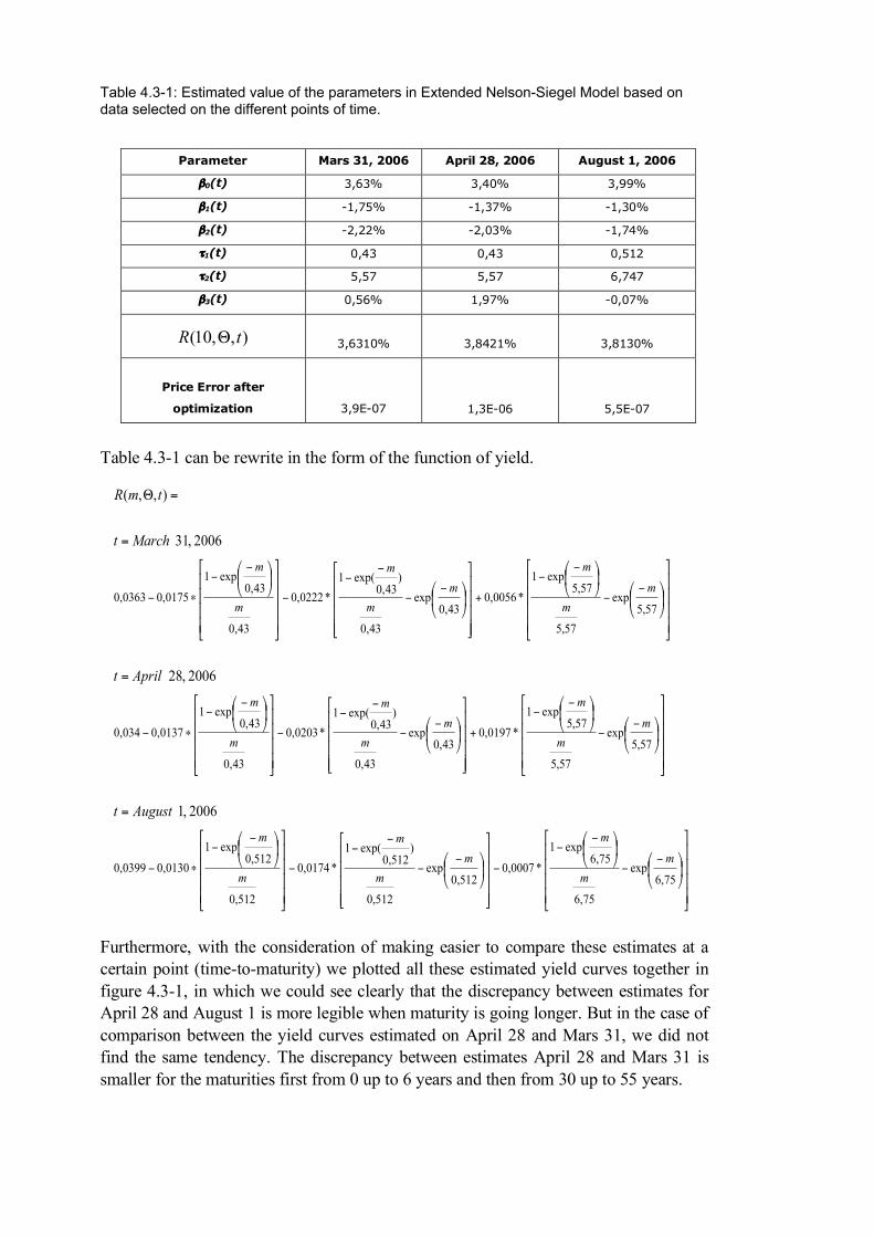
Furthermore, with the consideration of making easier to compare these estimates at acertain point (time-to-maturity) we plotted all these estimated yield curves together infigure 4.3-1, in which we could see clearly that the discrepancy between estimates forApril 28 and August 1 is more legible when maturity is going longer. But in the case ofcomparison between the yield curves estimated on April 28 and Mars 31, we did notfind the same tendency. The discrepancy between estimates April 28 and Mars 31 issmaller for the maturities first from 0 up to 6 years and then from 30 up to 55 years.
=
=
=
=Θ
−−
−−
−−
−
−−
−
−−
∗−
−−
−−
+−
−
−−
−
−−
∗−
−−
−−
+−
−
−−
−
−−
∗−
75,6exp
75,6
75,6exp1
*0007,0512,0
exp
512,0
)512,0
exp(1*0174,0
512,0
512,0exp1
0130,00399,0
57,5exp
57,5
57,5exp1
*0197,043,0
exp
43,0
)43,0
exp(1*0203,0
43,0
43,0exp1
0137,0034,0
57,5exp
57,5
57,5exp1
*0056,043,0
exp
43,0
)43,0
exp(1*0222,0
43,0
43,0exp1
0175,00363,0
2006 ,1
2006 ,28
2006 ,31
),,(
mm
mm
m
m
m
m
mm
mm
m
m
m
m
mm
mm
m
m
m
m
Augustt
Aprilt
Marcht
tmR
15
Figure 4.3-1: Yield curves estimated at the different points of time
4.4 IMPACT OF THE YIELD CURVES
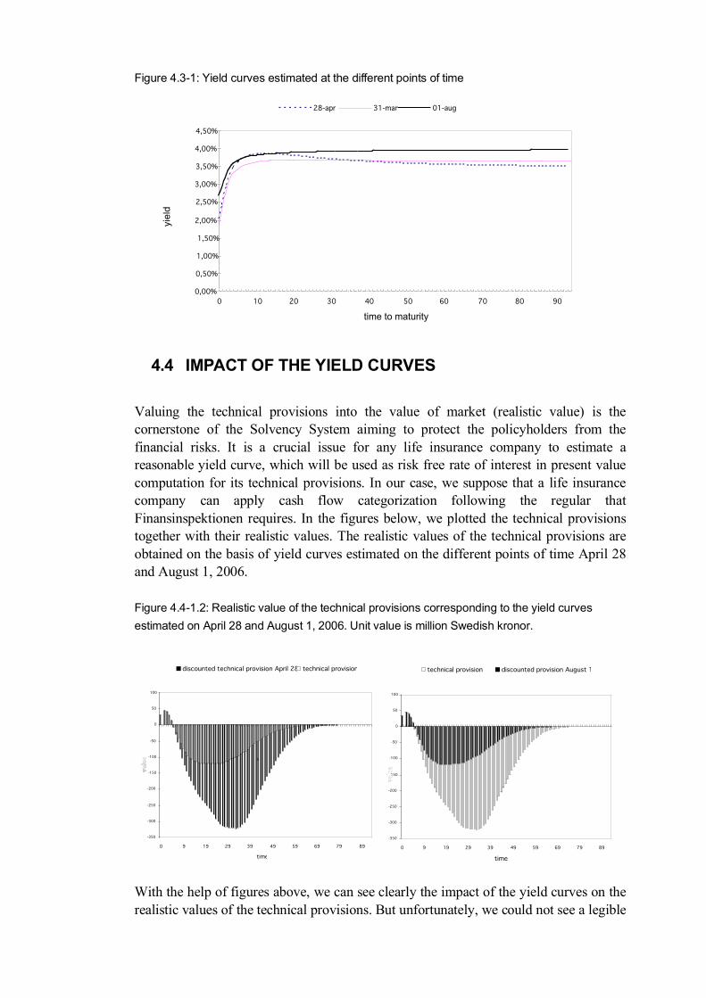
Valuing the technical provisions into the value of market (realistic value) is thecornerstone of the Solvency System aiming to protect the policyholders from thefinancial risks. It is a crucial issue for any life insurance company to estimate areasonable yield curve, which will be used as risk free rate of interest in present valuecomputation for its technical provisions. In our case, we suppose that a life insurancecompany can apply cash flow categorization following the regular thatFinansinspektionen requires. In the figures below, we plotted the technical provisionstogether with their realistic values. The realistic values of the technical provisions areobtained on the basis of yield curves estimated on the different points of time April 28and August 1, 2006.
Figure 4.4-1.2: Realistic value of the technical provisions corresponding to the yield curvesestimated on April 28 and August 1, 2006. Unit value is million Swedish kronor.
With the help of figures above, we can see clearly the impact of the yield curves on therealistic values of the technical provisions. But unfortunately, we could not see a legible
-350
-300
-250
-200
-150
-100
-50
0
50
100
0 9 19 29 39 49 59 69 79 89
time
discounted technical provision April 28 technical provision
5
-350
-300
-250
-200
-150
-100
-50
0
50
100
0 9 19 29 39 49 59 69 79 89
time
technical provision discounted provision August 1
0,00%
0,50%
1,00%
1,50%
2,00%
2,50%
3,00%
3,50%
4,00%
4,50%
0 10 20 30 40 50 60 70 80 90
time to maturity
yiel
d
28-apr 31-mar 01-aug
16
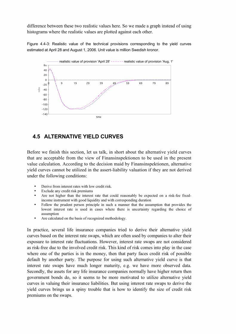
difference between these two realistic values here. So we made a graph instead of usinghistograms where the realistic values are plotted against each other.
Figure 4.4-3: Realistic value of the technical provisions corresponding to the yield curvesestimated at April 28 and August 1, 2006. Unit value is million Swedish kronor.
4.5 ALTERNATIVE YIELD CURVES
Before we finish this section, let us talk, in short about the alternative yield curvesthat are acceptable from the view of Finansinspektionen to be used in the presentvalue calculation. According to the decision maid by Finansinspektionen, alternativeyield curves cannot be utilized in the assert-liability valuation if they are not derivedunder the following conditions:
• Derive from interest rates with low credit risk.• Exclude any credit risk premiums• Are not higher than the interest rate that could reasonably be expected on a risk-fee fixed-
income instrument with good liquidity and with corresponding duration• Follow the prudent person principle in such a manner that the assumption that provides the
lowest interest rate is used in cases where there is uncertainty regarding the choice ofassumption
• Are calculated on the basis of recognized methodology.
In practice, several life insurance companies tried to derive their alternative yieldcurves based on the interest rate swaps, which are often used by companies to alter theirexposure to interest rate fluctuations. However, interest rate swaps are not consideredas risk-free due to the involved credit risk. This kind of risk comes into play in the casewhere one of the parties is in the money, then that party faces credit risk of possibledefault by another party. The purpose for using such alternative yield curve is thatinterest rate swaps have much longer maturity, e.g. we have more observed data.Secondly, the assets for any life insurance companies normally have higher return thengovernment bonds do, so it seems to be more motivated to utilize alternative yieldcurves in valuing their insurance liabilities. But using interest rate swaps to derive theyield curves brings us a spiny trouble that is how to identify the size of credit riskpremiums on the swaps.
-140
-120
-100
-80
-60
-40
-20
0
20
40
60
0 9 19 29 39 49 59 69 79 89
time
realistic value of provision 'April 28' realistic value of provision 'Aug, 1'
17
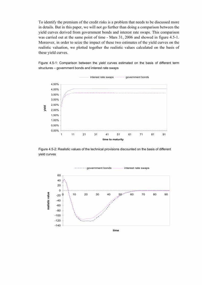
To identify the premium of the credit risks is a problem that needs to be discussed morein details. But in this paper, we will not go further than doing a comparison between theyield curves derived from government bonds and interest rate swaps. This comparisonwas carried out at the same point of time - Mars 31, 2006 and showed in figure 4.5-1.Moreover, in order to seize the impact of these two estimates of the yield curves on therealistic valuation, we plotted together the realistic values calculated on the basis ofthese yield curves.
Figure 4.5-1: Comparison between the yield curves estimated on the basis of different termstructures – government bonds and interest rate swaps
Figure 4.5-2: Realistic values of the technical provisions discounted on the basis of differentyield curves
0,00%
0,50%
1,00%
1,50%
2,00%
2,50%
3,00%
3,50%
4,00%
4,50%
1 11 21 31 41 51 61 71 81 91
time to maturity
yiel
d
interest rate swaps government bonds
-140
-120
-100
-80
-60
-40
-20
0
20
40
60
0 10 20 30 40 50 60 70 80 90
time
real
istic
val
ue
government bonds interest rate swaps
18
5 PARAMETRIC EFFECT ON THE YIELD CURVES
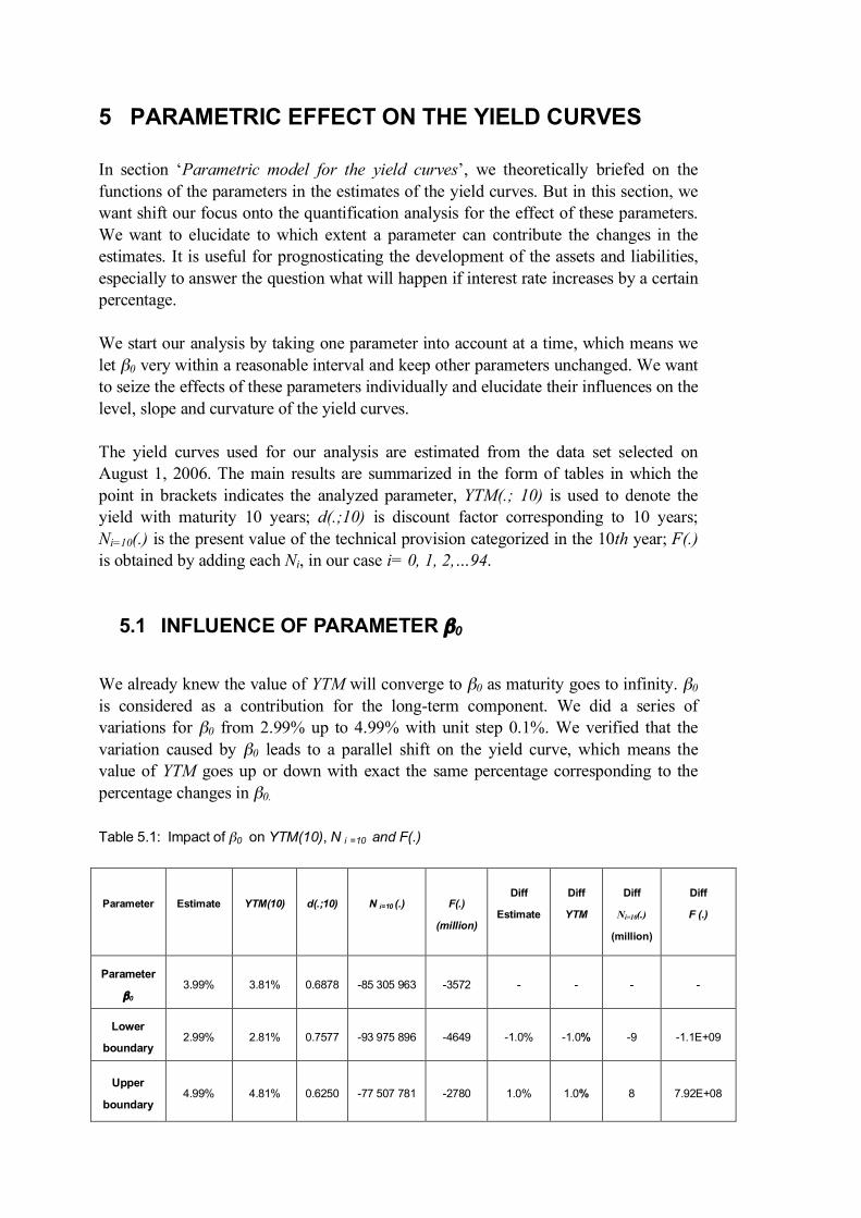
In section ‘Parametric model for the yield curves’, we theoretically briefed on thefunctions of the parameters in the estimates of the yield curves. But in this section, wewant shift our focus onto the quantification analysis for the effect of these parameters.We want to elucidate to which extent a parameter can contribute the changes in theestimates. It is useful for prognosticating the development of the assets and liabilities,especially to answer the question what will happen if interest rate increases by a certainpercentage.
We start our analysis by taking one parameter into account at a time, which means welet β0 very within a reasonable interval and keep other parameters unchanged. We wantto seize the effects of these parameters individually and elucidate their influences on thelevel, slope and curvature of the yield curves.
The yield curves used for our analysis are estimated from the data set selected onAugust 1, 2006. The main results are summarized in the form of tables in which thepoint in brackets indicates the analyzed parameter, YTM(.; 10) is used to denote theyield with maturity 10 years; d(.;10) is discount factor corresponding to 10 years;Ni=10(.) is the present value of the technical provision categorized in the 10th year; F(.)is obtained by adding each Ni, in our case i= 0, 1, 2,…94.
5.1 INFLUENCE OF PARAMETER β0
We already knew the value of YTM will converge to β0 as maturity goes to infinity. β0
is considered as a contribution for the long-term component. We did a series ofvariations for β0 from 2.99% up to 4.99% with unit step 0.1%. We verified that thevariation caused by β0 leads to a parallel shift on the yield curve, which means thevalue of YTM goes up or down with exact the same percentage corresponding to thepercentage changes in β0.
Table 5.1: Impact of β0 on YTM(10), N i =10 and F(.)
Parameter Estimate YTM(10) d(.;10) N i=10 (.) F(.)
(million)
Diff
Estimate
Diff
YTM
Diff
Ni=10(.)
(million)
Diff
F (.)
Parameter
β0
3.99% 3.81% 0.6878 -85 305 963 -3572 - - - -
Lower
boundary2.99% 2.81% 0.7577 -93 975 896 -4649 -1.0% -1.0% -9 -1.1E+09
Upper
boundary4.99% 4.81% 0.6250 -77 507 781 -2780 1.0% 1.0% 8 7.92E+08

19
Figure 5.1: The impact of β0 on the yield curves
5.2 INFLUENCE OF PARAMETER β1 AND τ1
An increment and reduction of β1 leads to a proportional increment and reduction ofYTM, respectively, but the magnitude of changes on YTM is smaller than what β0 did.An increment and reduction of τ1 makes a proportional reduction and increment onYTM, respectively, but the corresponding variation on YTM is much smaller than whatbeta parameters generated. But unfortunately, the impact of a combination of these twoparameters is hard to be quantified due to their adverse characteristics.
Table 5.2: Impact of β1 and τ1 on YTM(10) and Ni=10
Parameter (.) Estimate YTM(.;10) d(.;10) Ni=10 (.)Estimate
Diff
YTM(.;10)
Diff
Ni=10(.)
Diff
Parameter β1-1.30% 3.81% 0.6878 -85305963 - - -
Lower boundary -2.30% 3.76% 0.6912 -85727807 -1.00% -0.05% -421844
Upper boundary -0.10% 3.87% 0.6838 -84802762 1.20% 0.06% 503201
Parameter τ1 0.5120 3.81% 0.6878 -85305963 - - -
Lower boundary 0.1120 3.93% 0.6798 -84313751 -0.4000 0.12% 992212
Upper boundary 0.7220 3.75% 0.6921 -85831995 0.2100 -0.06% -526032
Combination of
β1 and τ1 (-1,30 ; 0,5120) 3.81% 0.6878 -85305963 - - -
Lower boundary (-2,30% ; 0,1120) 3.92% 0.6806 -84404638 (-1% ;-0.4) 0.11% 901325
Upper boundary (-0,10% ; 0,7220) 3.84% 0.6863 -85118531 (1.2% ; 0.21) 0.03% 187432
1 11 21 31 41 51 61 71 81 91
3,0%3,5%4,0%4,5%5,0%0,0%
0,5%
1,0%
1,5%
2,0%
2,5%
3,0%
3,5%
4,0%
4,5%
5,0%
YTM
time0β

20
Figure 5.2: The impact of β1 and τ1 on YTM(10).
5.3 INFLUENCE OF PARAMETERS β2 AND τ1
An increment and reduction of β2 leads to a proportional increment and reduction ofYTM, respectively, the magnitude of changes of YTM caused by this parameter is verysmall compared with what β0 did on the YTM. However, the impact of a combination ofparameters β2 and τ1 is hard to be quantified due to their adverse characteristics.
Table 5.3: Impact of β2 and τ1 on YTM(10) and Ni=10
Parameter Estimate YTM (.;10) d(.;10) Ni=10 (.) Estimate
Diff
YTM
Diff
Ni=10(.)
Diff
Parameter β2-1.74% 3.81% 0.6878 -85305963 - - -
Lower
boundary -2.74% 3.76% 0.6912 -85727807 -1.00% -0.05% -421844
Upper
boundary -0.64% 3.87% 0.6841 -84844571 1.10% 0.06% 461392
Parameter τ10.5120 3.81% 0.6878 -85305963 - - -
Lower
boundary 0.1120 3.93% 0.6798 -84313751 -0.4000 0.12% 992212
Upper
boundary 0.7220 3.75% 0.6921 -85831995 0.2100 -0.06% -526032
Combination
of β2 and τ1 (-1,74% ;0,5120) 3.81% 0.6878 -85305963 - - -
Lower
boundary (-2,74 ; 0,1120) 3.78% 0.6899 -85561170 (-1% ; -0.4) -0.03% -255207
Upper
boundary (-0,64% ;0,7220) 3.86% 0.6849 -84939618 (1.1% ; 0.21) 0.05% 366345
-2,30%-1,90%
-1,50%
-1,10%
-0,70%
-0,30%
0,1120,392
0,4320,472
0,5120,552
0,5920,632
0,6720,712
3,50%3,60%3,70%3,80%3,90%4,00%
YTM(10)
1β 1τ

21
Figure 5.3: The impact of β2 and τ1 on YTM(10)
5.4 INFLUENCE OF PARAMETERS β3 AND τ2
A series of variations has been maid on the parameters β3 and τ2. An increment andreduction of β3 leads to a proportional increment and reduction of YTM, respectively.But the magnitude of changes in YTM(10) corresponding to the effect of β3 isconsiderably small. In the case of τ2, an increment and reduction of it does not make acorresponding linear variation of YTM, and moreover the magnitude of changes ofYTM(10) effected by the variation of τ2 is extremely small. Figure 5.4 showed us whatkind of impact that τ2 has on Ni=10. To quantify the impact of these parameters’combination is a delicate matter in the sense that parameter τ2 has a complicatedproperty.
Table 5.4: Impact of β3 and τ2 on YTM(10) and Ni=10
Parameter Estimate YTM(.;10) d(.;10) Ni =10 (.) Estimate
Diff
YTM(.;10)
Diff
Ni =10 (.)
Diff
Parameter β3 -0.07% 3.81% 0.6878 -85305963 - - -
Lower boundary -2.07% 3.22% 0.7281 -90296746 -2.00% -0.59% -4990783
Upper boundary 2.53% 4.58% 0.6391 -79266073 2.60% 0.77% 6039890
Parameter τ2 6.75 3.810% 0.6878 -85305963 - - -
Lower boundary 1.75 3.822% 0.685 -85231830 -5.00 0.012% 74133
Upper boundary 11.75 3.817% 0.6843 -85277177 5.00 0.007% 28786
Combination of β3 and τ2 (-0,07% ; 6,75) 3.81% 0.6878 -85305963 - - -
Lower boundary (-2,07% ; 1,75) 3.48% 0.7103 -88089233 (-2.0% ; -5) -0.33% -2783270
Upper boundary (2,53% ; 11,75) 4.46% 0.6466 -80189361 (2.6% ; 5) 0.65% 5116602
3,60%
3,70%
3,80%
3,90%
YTM(10)
2β 1τ

22
Figure 5.4: The impact of β3 and τ2 on N i=10 . Unit value is million Swedish kronor.
-95
-90
-85
-80
-75
-70Value
β3
τ2
-95
-90
-85
-80
-75
-70
Value
3β2τ

23
6 LIFE INSURANCE MATHEMATICS6.1 PENSION SYSTEM IN SWEDEN
A pyramid with three layers can generalize the Swedish pension system (see the figure6.1 below). The basis of the pyramid is national pension, interlayer is occupationalpension and the top-level is private pension. The national pension is a statutorypension, which is paid out by the National Insurance Office. Individuals earn money fortheir national pension during their entire life. The old system (basic pension andnational supplementary pension) remains for people born in 1937 or earlier. The newpension system covers people born in 1938 or later and started to pay out pension in2003. The national pension comprises three components: income pension, premiumpension and guarantee pension. Occupational pension is built up on an agreementbetween trade unions and employers for the benefit of the employees, and paid out bydifferent pension institutions, depending on whether you work within private industry,local government/county council etc. Generally the occupational pensionapproximately amounts to 10 per cent of salary at the year before he/she retires onhis/her pension. The total period of employment, moreover, affects the outcome ofoccupational pension. Individuals create private pension savings as supplement fortheir pension. There are several life insurance products that people can choose to fittheir own life situation, such as traditional pension insurance, unit-link fund insuranceand ordinary savings.
Figure6.1: Swedish pension system shaped in a form of pyramid.
6.2 LIFE INSURANCE RISKS
As we mentioned before in section one ‘Interest rate risk in the focus’,Finansinspektionen emphasizes that each transaction in an insurance contract mustessentially be discounted individually using the risk-free rate of interest thatcorrespond to the duration of the liabilities.
In reality, it’s not easy for a life insurance company to evaluate these futuretransactions exactly, because the magnitude of in- and out-cash flows are notdetermined. Quantifying the changes that could be caused by the decisions made frominsurers and policyholders requires a more complicated calculating approach in whichdistribution of profit, requirement of repayment cover etc. can be taken into account.
Occupational pension
National pension (Income-, premium- and guarantee pension)
Private pension
24
In this paper we don’t keep our focus on risk factor identification, but how to quantifythese uncertainties. Furthermore, we are not going to discus all factors that possiblyhave statistical effects on valuing cash flows, it will be impossible with theconsideration of paper space. We decided to discuss risks that have a great deal ofimpact on life assurance mathematics.
Transfer risk: A policyholder signs up for a certain insurance contract period butchanges his mind after a while and wants his accumulated capital transferred to anotherinsurance company before the maturity date of the policy. This is defined as transferrisk. It should be noted that surrender is a term most often for life policies but transfermight often have the same economic impact on the insurance business. In this paper wehave not taken transfer risk into account.
Paid-up risk: Another possible opportunity for those who wish to discontinuepremium payment is the paid-up policy. Such a policy remains in-force but no furtherpremiums will be paid in. In practice, using a standard paid-up assumption seems to bea solution to deal with such problems, e.g. each year a certain percentage of policieswith regular premiums will be converted to paid-up.
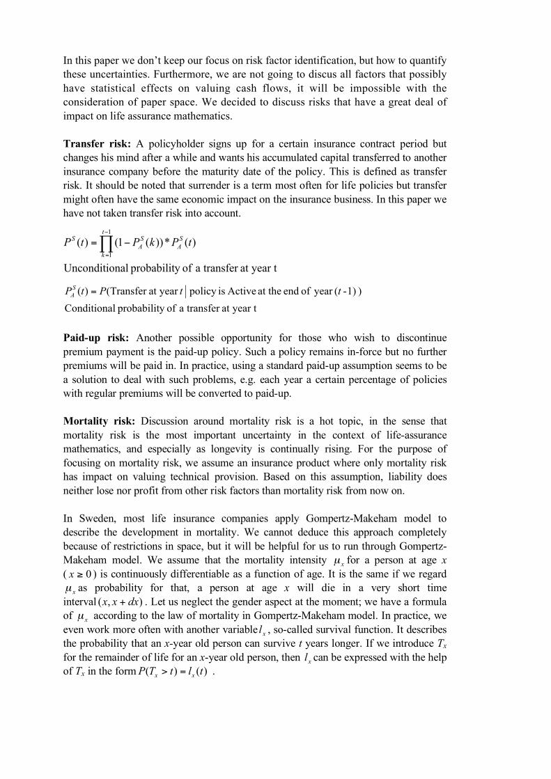
Mortality risk: Discussion around mortality risk is a hot topic, in the sense thatmortality risk is the most important uncertainty in the context of life-assurancemathematics, and especially as longevity is continually rising. For the purpose offocusing on mortality risk, we assume an insurance product where only mortality riskhas impact on valuing technical provision. Based on this assumption, liability doesneither lose nor profit from other risk factors than mortality risk from now on.
In Sweden, most life insurance companies apply Gompertz-Makeham model todescribe the development in mortality. We cannot deduce this approach completelybecause of restrictions in space, but it will be helpful for us to run through Gompertz-Makeham model. We assume that the mortality intensity xµ for a person at age x( 0≥x ) is continuously differentiable as a function of age. It is the same if we regardxµ as probability for that, a person at age x will die in a very short time
interval ),( dxxx + . Let us neglect the gender aspect at the moment; we have a formulaof xµ according to the law of mortality in Gompertz-Makeham model. In practice, weeven work more often with another variable xl , so-called survival function. It describesthe probability that an x-year old person can survive t years longer. If we introduce Tx
for the remainder of life for an x-year old person, then xl can be expressed with the helpof Tx in the form )()( tltTP xx => .
year tat transfer a ofy probabilit lConditiona) 1)-(year of end at the Active ispolicy year at Transfer ()( ttPtPSA =
year tat transfer a ofy probabilit nalUnconditio
)(*))(1()(1
1∏−
=
−=t
k
SA
SA
S tPkPtP

25
0 t where)(
)()(
person oldyear an for life ofremainder where )()(
)(')( and 0 where)(1
)(
)(
0
0
x
≥∫
=+
=
=≤=
=≥−
=⋅+=
+−
⋅
tx
xdss
x
xx
xx
exltxltl
xTtTPtF
xFxfxxFxfe
µ
γβαµ
With the specification in the current official Swedish mortality table M90, we have theexplicit formula for mortality intensity, which is utilized also in this paper.
In practice, commutation functions D (x) and N (x) are introduced into valuingprovision for the purpose of reducing complexities. D (x) and N (x) are defined asbelow
In this paper, out-cash flow in a life insurance company is approximately equal to theexpected value of benefit on the collective level, which will be paid out from thecompany successively in the future. We also assume that in-cash flow is equal to theexpected value of premium on the same level as benefit, which will be paid in frompolicyholders successively during the signed contract period. Net cash flow is simplyequal to the difference between the out- and in-cash flows under the condition thatpolicyholders are alive during this period.
6.3 CASH FLOW VALUATION
We start with a simple insurance product for the needs of occupational pension,wherein benefit S will be paid out successively to a policyholder at the year from whichhe has reached 65, as long as he is alive but no longer than 5 years. During the signedcontract period, the policyholder will pay his premium until he is 65. Our policyholderhere is 60 years old at the point of time t when the calculation is carried out.
At the point of time t, out- and in-cash flows for a policyholder are calculated by theformulas below.
ly respective women andmen for 6,or 0 0.044 and 0.000012 0.001, ,0 where,
)()10ln(
=
===≥
⋅+= −⋅⋅
fx
e fxx
γβα
βαµ γ
deduction tax ofeffect tax and ratediscount is )charge premium()tax1ln(by determined factor,discount is ,where
)()( ,)()(
rr
duuDxNexlxDx
x
−⋅+
=⋅= ∫∞
⋅−
δ
δ

26
It should be noted that functions a(t) and b(t) are not directly dependent on t, but theage of our policyholder at the time point t. At the point of time t, the calculation of out-and in-cash flow on the collective level can be carried out in a similar way. In theformula below, w(60) is denoted for a total number of individuals who are 60 years oldin the year of calculation and they have exactly the same insurance contract.
Formulas above give us a comprehensive view of development of benefit and premiumfrom statistic perspective, but now we want to shift our focus into technical detail,which means the formula will be deduced in a discrete context.
We can even more develop the function above under a condition that pension will bepaid out from the insurance company to the policyholder in the beginning of each year.
Furthermore, let V (t) denote the present value of net cash flows in a life insurancecompany at point of time t, e.g. V (t) =B (t) - A (t).
)60(
)(a(t)
)60()65()60(a(t) flowcash in
)60(
)( b(t)
)60()70()65(b(t) flowcash out
65
60
70
65
tt
t
tt
D
duuDPP
DNN
D
duuDSS
DNN
∫
∫
∗=⇔∗−
=−
∗=⇔∗−
=−
)60()60(
)65()60( A(t) flowcash in
)60()60(
)70()65(B(t) flowcash out
wPD
NN
wSD
NN
t
t
t
∗∗−
=−
∗∗−
=−
)60()70()69(
)60()67()66(
)60()66()65(
)60()70()65(
tttt DNN
DNN
DNN
DNN −
++−
+−
=−
L
965
)60()69(
)60()66(
)60()65(
)60()70()69(
)60()67()66(
)60()66()65(
)60()70()65(
⋅−⋅−⋅− ⋅++⋅+⋅=
−++
−+
−=
−
δδδ elle
lle
ll
DNN
DNN
DNN
DNN
ttt
tttt
L
L
27
7 PROBLEM OF MISMATCH
7.1 MISMATCH BETWEEN THE ASSET AND THE LIABILITY
Mismatching between the assets and the liabilities is a very problematic issue in thefinancial area because it has a multiple property. Mismatching in a life insurancecompany is sculptured out of life insurance mathematics due to the actuarialassumptions made in insurance subsidiaries. A traditional way to scrutinize thisproblem is to partition it into segments, in which the assets and liabilities aremismatched. It should be noted that in this paper the mismatching problem has beenlocalized on the level where we are supposed to get a suitable balance between therestricted assets and the technical provisions.
Let us for the moment leave the provisions aside and concentrate upon the restrictedassets. For an asset portfolio consists of interest rate instruments, there are at least threemismatched segments that a life actuary must to take into account. These segments aremismatched present values, durations and liquidities. As a well known financialsolution, immunization has been used to reduce the impact of interest rate fluctuationsthat generate the mismatch in the present value and duration. By the help of thisapproach, these two mismatched segments can successfully bridged over, we can evenget a better match between the assets and liabilities if their convexities could be equal.But unfortunately, the immunization cannot contribute anything for solving themismatch in the liquidity, which means at a certain moment the value of asset portfoliois not enough for the liabilities or adversely much more than necessary. Both situationswill cost a company huge money, because the first possibility will force an insurer tomake credits, and in the case of temporary surplus, we have to keep them under themattress to fit the future payments. A possible compensation for immunization is tohave a buffer capital for such happenings.
For an asset portfolio consists of more than interest rate instruments, for instance,shares and properties, ALM (Asset-Liability Model) seems to be a reasonable approachto deal with the problem of mismatch. ALM is a modeling trying to capture thestochastic uncertainties involved in the assets and liabilities. It provides the insurers asolution in which they have a dynamic control over the development of their assets andliabilities, provided that the structure of the assets and liabilities are unchanged throughthe ages. However, the reality for a life insurer is much more complicated in the sensethat the actuarial assumptions do change over time. There is limitation in ALM to keepup a correspondence to such uncertainties. A possible compensation for the ALM is tobuild up a realistic model for the in- and out- cash flows in a life insurance company.This model will reflect all uncertainties hid behind the assets and insurance liabilities,e.g. the financial, operational and insurance risks.
7.2 THE RESTRICTED ASSETS
Building up a realistic model is out of this work because the object of this paper isprotecting the guaranteed undertakings from the interest rate risk with a high degree of

28
certainty, which means the asset portfolio is not designed for a better return butmatching the guaranteed undertakings. A portfolio consists of only governments bondsshould be suitable for this purpose. It would be easy for us to solve the problem if themethod of immunization can be applied in this case, but unfortunately this approach isnot available due to the short maturities (almost 15 years for the longest one) thatSwedish government bonds have.
Our strategy for solving the mismatch problem is creating an asset portfolio whose cashflows are distributed more like our insurance liabilities; furthermore the portfolio isexpected to have more tolerance to the interest rate fluctuations. The point of departureis testing reasonable combinations of bonds that could satisfy our requirements above.We decided to have an asset portfolio that consists of government bonds SO-1037,1040, 1045, 1049 and 1047 with the consideration of their different long durations.Based on the tests we finally managed up an asset portfolio where the magnitudes ofeach bond is given to 2400, 1800, 400, 300 and 225 standard respectively. Table 7.2-1listed the present value of our assets that are designed to cover our determined technicalprovisions. The present value calculation is carried out on the basis of three estimatedyield curves. Two scenarios - buffer capital and solvency ratio are introduced todescribe the positions of our restricted assets and technical provisions. The value of ourbuffer capital is obtained by adding the present values of the assets and provisions.Solvency ratio is equal to the absolute value of the division between the realistic valueof the restricted assets and technical provisions. PV stands here for the realistic values.
Table7.2-1: Realistic values of restricted assets and technical provisions calculated on thebasis of different yield curves. Unit value is milliard Swedish kronor.
Mars 31 April 28 August 1
YTM(10) 3.6310% 3.8421% 3.8130%
PV (provisions) -3,804 -3,768 -3,572
PV (restricted assets) 5,583 5,580 5,543
SO-1037 2400 2400 2400
SO-1040 1800 1800 1800SO-1045 400 400 400SO-1049 300 300 300SO-1047 225 225 225
Buffer capital 1,780 1,812 1,971Solvency ratio 1.47 1.48 1.55
Based on the earlier studies we know that the changes in the yield curves made the lifeinsurance companies vulnerable due to the long duration for their insurance liabilities.With the help of Extended Nelson-Siegel modeling, we are capable to carry out a stresstest on the yield curves aiming to prognosticating the development of our assets andliabilities corresponding to the changes in interest rates.
In the stress test, we made a series of paralleled shifts on each of original yield curvesestimated on the different time points. The magnitude of each shift is 5 basis points

29
(5bp = 0.05%). Our created asset portfolio passed the stress tests by a good tolerancefor a broad paralleled shift (from -150bp to +150bp) on the yield curves.
A part of results of stress tests is showed in the tables below in which we found thateach +50bp stressed on these yield curves leads to a reduction by about 20 percent forthe solvency ratio; each -50bp stressed for the curves gives an increment by about 16percent for the solvency ratio. The most important signal for a life insurance companyis the solvency ratio getting close to the crucial level 1 when the interest rate goingdown with 1%.
Table7.2-2: Paralleled shift by ± 50bp stressed on the different yield curves. Unit value ismilliard Swedish kronor.
+50bp -50bp
Mars 31 April 28 August 1 Mars 31 April 28 August 1
YTM(10) 4,1310% 4,3421% 4,3130% 3,1310% 3,3421% 3,3130%
Paralleled shift 0,5000% 0,5000% 0,5000% -0,5000% -0,5000% -0,5000%
PV(provisions) -3, 344 -3, 309 -3, 146 -4, 341 -4, 304 -4, 068
PV(restricted assets) 5, 535 5, 535 5, 495 5, 633 5, 628 5, 593
SO-1037 2400 2400 2400 2400 2400 2400
SO-1040 1800 1800 1800 1800 1800 1800
SO-1045 400 400 400 400 400 400SO-1049 300 300 300 300 300 300SO-1047 225 225 225 225 225 225
Buffer capital 2,191 2,225 2,349 1, 292 1, 323 1, 525Solvency ratio 1,66 1,67 1,75 1,30 1,31 1,37
Table7.2-3: Paralleled shift by 100bp stressed on the different yield curves. Unit value ismilliard Swedish kronor.
+100bp -100bp
Mars 31 April 28 August 1 Mars 31 April 28 August 1
YTM (10) 4,6310% 4,8421% 4,8130% 2,6310% 2,8421% 2,8130%
Paralleled shift 1,0000% 1,0000% 1,0000% -1,0000% -1,0000% -1,0000%
PV (provision) -2, 949 -2, 916 -2, 780 -4, 972 -4, 935 -4, 649
PV (restricted assets) 5, 489 5, 490 5, 449 5, 685 5, 677 5, 644
SO-1037 2400 2400 2400 2400 2400 2400SO-1040 1800 1800 1800 1800 1800 1800SO-1045 400 400 400 400 400 400SO-1049 300 300 300 300 300 300SO-1047 225 225 225 225 225 225
Buffer capital 2, 540 2, 575 2, 670 0, 714 0, 742 0, 995
Solvency ratio 1,86 1,88 1,96 1,14 1,15 1,21
30
7.3 SENSITIVITY TO THE INTEREST RATE RISK
Even though the method of immunization cannot be applied in our case, it is stillimportant for an actuary to control how the restricted assets, technical provisions andbuffer capital behave corresponding to the changes in interest rate.
We already know from section ‘Term structure of interest rate’, duration and convexityare two powerful risk measures that can be used to assess the interest rate risk. Durationprovides the information about the slope of the line tangent to the price -yield curve at acertain point, and its magnitude is ( PD ified ∗− mod ). With the help of convexity we canget even better approximation for the price-yield curve because it provides the relativecurvature at a given point on the curve.
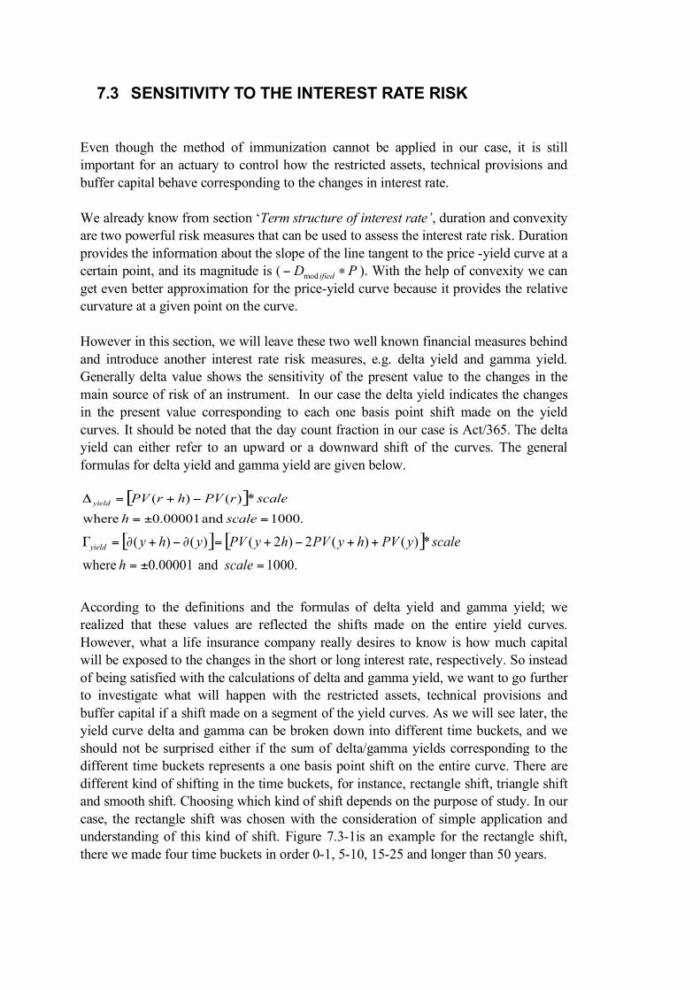
However in this section, we will leave these two well known financial measures behindand introduce another interest rate risk measures, e.g. delta yield and gamma yield.Generally delta value shows the sensitivity of the present value to the changes in themain source of risk of an instrument. In our case the delta yield indicates the changesin the present value corresponding to each one basis point shift made on the yieldcurves. It should be noted that the day count fraction in our case is Act/365. The deltayield can either refer to an upward or a downward shift of the curves. The generalformulas for delta yield and gamma yield are given below.
[ ].1000 and 00001.0 where
*)()(
=±=
−+=Δ
scalehscalerPVhrPVyield
[ ] [ ].1000 and 00001.0 where
*)()(2)2()()(
=±=
++−+=∂−+∂=Γ
scalehscaleyPVhyPVhyPVyhyyield
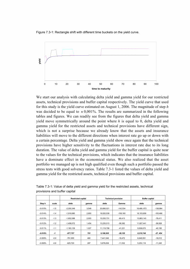
According to the definitions and the formulas of delta yield and gamma yield; werealized that these values are reflected the shifts made on the entire yield curves.However, what a life insurance company really desires to know is how much capitalwill be exposed to the changes in the short or long interest rate, respectively. So insteadof being satisfied with the calculations of delta and gamma yield, we want to go furtherto investigate what will happen with the restricted assets, technical provisions andbuffer capital if a shift made on a segment of the yield curves. As we will see later, theyield curve delta and gamma can be broken down into different time buckets, and weshould not be surprised either if the sum of delta/gamma yields corresponding to thedifferent time buckets represents a one basis point shift on the entire curve. There aredifferent kind of shifting in the time buckets, for instance, rectangle shift, triangle shiftand smooth shift. Choosing which kind of shift depends on the purpose of study. In ourcase, the rectangle shift was chosen with the consideration of simple application andunderstanding of this kind of shift. Figure 7.3-1is an example for the rectangle shift,there we made four time buckets in order 0-1, 5-10, 15-25 and longer than 50 years.
31
Figure 7.3-1: Rectangle shift with different time buckets on the yield curve.
0 10 20 30 40 50 60 70 80 90 100
time to maturity
yiel
d
We start our analysis with calculating delta yield and gamma yield for our restrictedassets, technical provisions and buffer capital respectively. The yield curve that usedfor this study is the yield curve estimated on August 1, 2006. The magnitude of step hwas decided to be equal to ± 0,001%. The results are summarized in the followingtables and figures. We can readily see from the figures that delta yield and gammayield move symmetrically around the point where h is equal to 0, delta yield andgamma yield for the restricted assets and technical provisions have different sign,which is not a surprise because we already know that the assets and insuranceliabilities will move to the different directions when interest rate go up or down witha certain percentage. Delta yield and gamma yield show once again that the technicalprovisions have higher sensitivity to the fluctuations in interest rate due to its longduration. The value of delta yield and gamma yield for the buffer capital is quite nearto the values for the technical provisions, which indicates that the insurance liabilitieshave a dominate effect in the economical status. We also realized that the assetportfolio we managed up is not high qualified even though such a portfolio passed thestress tests with good solvency ratios. Table 7.3-1 listed the values of delta yield andgamma yield for the restricted assets, technical provisions and buffer capital.
Table 7.3-1: Value of delta yield and gamma yield for the restricted assets, technicalprovisions and buffer capital
Restricted capital Technical provision Buffer capital
Step h scale delta gamma delta Gamma delta gamma
-0.015% -1.5 -2,200,349 3,549 20,690,021 -142,534 18,489, 672 -138,984
-0.014% -1.4 -1,916,680 2,693 18,020,539 -108,160 16,103,859 -105,466
-0.013% -1.3 -1,652,588 2,003 15,535,731 -80,413 13,883,143 -78,411
-0.012% -1.2 -1,408,072 1,454 13,235,513 -58,382 11,827,441 -56,928
-0.011% -1.1 -1,183,129 1,027 11,119,799 -41,221 9,936,670 -40,195
-0.010% -1 -977,757 701 9,188,505 -28,155 8,210,748 -27, 454
-0.009% -0.9 -791,955 460 7,441,546 -18,472 6,649,591 -18,012
-0.008% -0.8 -625,720 287 5,878,838 -11,532 5,253,118 -11,245

32
-0.007% -0.7 -479,050 168 4,500,294 -6,760 4,021,244 -6,592
-0.006% -0.6 -351,942 91 3,305,831 -3,649 2,953,889 -3,558
-0.005% -0.5 -244,396 44 2,295,364 -1,760 2,050,968 -1,716
-0.004% -0.4 -156,408 18 1,468,807 -721 1,312,400 -703
-0.003% -0.3 -87,976 6 826,077 -228 738,101 -222
-0.002% -0.2 -39,099 1 367,089 -45 327,990 -44
-0.001% -0.1 -9,774 0.07 91,758 -3 81,984 -3
0.000% 0 0 0.00 0 0 0 0
0.001% 0.1 -9,774 0.07 91,730 -3 81,956 -3
0.002% 0.2 -39,093 1 366,864 -45 327,770 -44
0.003% 0.3 -87,957 6 825,317 -228 737,360 -222
0.004% 0.4 -156,363 18 1,467,005 -721 1,310,643 -703
0.005% 0.5 -244,308 44 2,291,844 -1,760 2,047,536 -1,716
0.006% 0.6 -351,791 91 3,299,749 -3,649 2 947 959 -3,558
0.007% 0.7 -478,809 168 4,490,637 -6,760 4,011,828 -6,592
0.008% 0.8 -625,361 287 5,864,422 -11,532 5,239,061 -11,245
0.009% 0.9 -791,444 460 7,421,022 -18,472 6,629,578 -18,012
0.010% 1 -977,056 701 9,160,351 -28,155 8,183,294 -27, 454
0.011% 1.1 -1,182,196 1,027 11,082,325 -41,221 9,900,129 -40,195
0.012% 1.2 -1,406,860 1,454 13,186,861 -58,382 11,780,001 -56,928
0.013% 1.3 -1,651,048 2,003 15,473,875 -80,413 13,822,827 -78,411
0.014% 1.4 -1,914,756 2,693 17,943,282 -108,160 16,028,526 -105,466
0.015% 1.5 -2,197,983 3,549 20,594,999 -142,534 18,397,016 -138,984
In the analysis of shifting segments of the yield curve, we did the following restrictionsto simplify the calculations. We decided to make a shift with magnitude one basispoint, and moreover we chose the underlying capital in our analysis to be the net cashflows that indicate how much capitals are available at each point of time. Wesummarized our results in table 7.3-2. If we compare the result with the values that weobtained for the buffer capital, (delta yield =8 183 294 and gamma yield = -27 454, seetable 7.3-1), we realized these values are quite close to each other. It verified that ourstatement made earlier in this section, the sum of different time buckets shouldrepresent the shift on the whole yield curve.
Table7.3-2: Investigation summary for sifting segments of the yield curve with one basis point
Time bucket (year) Delta yield Gamma yield
0-1 -19,701 4
1-2 364,118 106
2-5 -217,063 120
5-10 5,702 -23
10-15 637,292 -911
15-25 2,124,773 -4,560
25-50 5,476,851 -19,365
>50 514,578 -2,808
Total value 8,158,313 27,437

33
Based on table 7.3-1, we made up figures 7.3-2 where we put together the delta yieldfor the restricted assets, technical provisions and buffer capital. In figure 7.3-3 we puttogether their gamma yield. The purpose for doing so is to describe the financial riskstatus for a life insurance company. It is useful for an actuary to have suchinformation besides the balance sheet, so he or she can possibly have a whole pictureof the economic growth for his or her company. As we mentioned in the verybeginning of this paper, the cornerstone of the Traffic Light System is to protectpolicyholders from the financial uncertainties and in our case especially to protectthem from the interest rate fluctuations.
Figure 7.3-2: Delta yield for the restricted assets, technical provisions and buffer capital. Unitvalue is million Swedish kronor
-5
0
5
10
15
20
25
-0,01
5%
-0,01
4%
-0,01
3%
-0,01
2%
-0,01
1%
-0,01
0%
-0,00
9%
-0,00
8%
-0,00
7%
-0,00
6%
-0,00
5%
-0,00
4%
-0,00
3%
-0,00
2%
-0,00
1%
0,000
%
0,001
%
0,002
%
0,003
%
0,004
%
0,005
%
0,006
%
0,007
%
0,008
%
0,009
%
0,010
%
0,011
%
0,012
%
0,013
%
0,014
%
0,015
%
h
delta
yie
ld
delta asset delta liability delta buffer capital
Figure7.3-3: Gamma yield for the restricted assets, technical provisions and buffer capital.Unite value is thousands Swedish kronor
-160
-140
-120
-100
-80
-60
-40
-20
0
20 -0,
015%
-0,01
4%
-0,01
3%
-0,01
2%
-0,01
1%
-0,01
0%
-0,00
9%
-0,00
8%
-0,00
7%
-0,00
6%
-0,00
5%
-0,00
4%
-0,00
3%
-0,00
2%
-0,00
1%
0,000
%
0,001
%
0,002
%
0,003
%
0,004
%
0,005
%
0,006
%
0,007
%
0,008
%
0,009
%
0,010
%
0,011
%
0,012
%
0,013
%
0,014
%
0,015
%
h
gam
ma
yiel
d
gamma liability gamma buffer capital gamma asset

34
8 CONCLUSION
Every insurer desires to have the suitable balance between the assets and liabilitiesaiming to improve growth, profit and risk control. An insurer may be exposed to manydifferent types of risks, and the unique one amongst them is insurance risk. It requiresan insurer to utilize a specific risk-control method that differs from the general financialmanagement. As a response to the IORP Directive, the Traffic Light System is assignedby the Swedish Financial Supervisory Authority to obtain more complete control overthe life insurers in Sweden.
This paper examines the impact of interest rate risk on the life insurance assets andliabilities. The main work has been estimating the yield curves and sensitivity testing.Stress test of interest rates has been applied for this purpose in order to achieve asuitable balance between the assets and liabilities in such a way that fluctuations ininterest rates by shifts do not affect the financing of liabilities.
The technical provisions have been valued at their realistic value, which means at everygiven point of time the technical provisions have been discounted on the basis of ayield curve estimated by Extended Nelson Siegel model. Four yield curves (estimatedon the different point of time and underlying instruments) have been applied in ouranalysis. The results delivered from these curves showed that the estimates are timedependent. Furthermore as a consequence of the dependency, the estimates have a greatimpact on the realistic value of our technical provisions. It motivates the requirementfrom the Swedish authority about estimating reasonable discount rates.
As we mentioned in the beginning of this paper, our focus is interest rate risk. Thatmeans mismatch between life insurance assets and liabilities caused by interest ratefluctuations is the issue for this paper. Several stress tests have been applied forinvestigating the problem. Based on the portfolio assigned for the restricted assets, wecarried out stress tests to see if such a portfolio will exceed the required solvency ratio.The results showed that the created portfolio has good tolerance for the paralleled shift(from -150 bp up to +150 bp) on the entire yield curves. However, the solvency ratiowill get close to the crucial level when the interest rates are going down with onepercentage.
Stress tests are considered as a tool for examining what might happen in a particularstress scenario. However, it should be noted that stress tests do not predict what willhappen. Moreover, stress tests are not suitable approaches for an insurer who expects toapply techniques that are appropriate for the whole risk profile and the businessundertaken. We have mentioned before in section ‘Life insurance mathematics’, webelieve a complex realistic modeling should be an appropriate tool for the life insurers.
Furthermore, for the purpose of analyzing the interest rate risk, we decided to havesimple structure for both insurance assets and liabilities. However, with theconsideration of life insurers’ reality, the technical provisions might be calculated insuch a way that they could reflect the reality of the insurance contracts. In the case of

35
the restricted assets, their simple structure made extremely difficult for insurers toobtain a suitable balance aiming to improve their risk control. A following work afterthis paper could be to create a realistic portfolio with more complex structure for therestricted assets, shares and interest rate swaps could be considered in such a case.
36
9 REFERENCES
Jan R. M. Röman (2006). Lecture notes in Analytical Finance I & II,Department of Mathematics and Physics, Mälardalen University, Sweden
Thomas Höglund (2005). Lecture notes in Finance mathematics I & II,Mathematical Statistical Institute at Stockholm University, Sweden
C.R. Nelson and A.F. Segel (1987). Parsimonious Modelling of Yield Curves,Journal of Busniness, 60:473-89.
Lars E.O. Svensson (1994).Estimating and Interpreting Forward Interest Rates: Sweden 1992-1994,NBER Working Paper Series, No.4871.
David G. Luenberger (1998). Investment Science, Oxford University Press
Bank of International Settlements (October, 2005).Zero-coupon yield curves: technical documentation,BIS Papers No 25, Monetary and Economic Department.
Deutsche Bundesbank (October, 1997). Estimating the term structure of interest rates,Monthly Report
Yu, I. y Fung, L. (2002).Estimation of Zero-Coupon Yield Curves Based on Exchange Fund Bills and Notes in HongKong, Market Research Division, Research Department, Hong Kong Monetary Authority.
Gunnar Andersson (2005). Livförsäkringsmatematik I.
Erik Alm, Gunnar Andersson, Bengt von Bahr and Anders Martin Löf (2006).Livförsäkringsmatematik II
Björn Palmgren (August, 2000).Preliminary discussion note on cash-flow analysis in insurance (In Swedish).
The Swedish Financial Supervisory Authority (2006).Tjänstepensionföretag – en vägledning, 2006-05-22
The Swedish Financial Supervisory Authority (2005).Trafikljusmodellen – Beslutad version, 2005-11-08

37
The Swedish Financial Supervisory Authority (2005).Memorandum: Discount rates, 2005-11-08
International Association of Insurance Supervisors (2006).Asset Liability Management, Issues paper 31 May.
Statens Offentliga Utredningar, 2003:84

38
10 APPENDIX
• The yield function ),,( tmR Θ in Nelson-Siegel model
• The form of Extension Temporary Pension in a discrete context
−−
⋅+
−⋅+=
−+−⋅⋅+−⋅⋅+=
⋅⋅
+⋅
+=
⋅⋅++=
===
−⋅+
−⋅+
=
−⋅+−⋅+=
Θ=Θ
∫−−
∫∫
∫∫
∫
∫
∫
∫
∫
−
−−
−−
)exp()exp(1)exp(1
,
)exp(1
)exp(1
1
)exp()exp(1
),,(1),,(
,1,1
,1,2
,1
,1,1,0
00
,1,2
0
,1,1,0
0
,1,2
0
,1,1,0
0,1
,2
0,1
,1,0
,1,1
0 ,1,1,2
0 ,1,1
0,0
0 ,1,1,2
,1,1,0
0
,1,1,1
,1,1
,1,1
tt
tt
t
ttt
m
y
m
tt
m
ttt
m
ytt
m
yttt
m
yt
t
m
yt
tt
tt
m
ttt
m
tt
m
t
m
ttt
ttt
m
mm
m
m
m
dyeym
ym
dyeym
dyem
dyeym
dyem
dydxxy
dxxxm
dxxm
dxm
dxxxxm
dxtxfm
tmR
ttt
tt
tt
yee
ττ
τβ
τ
τββ
τβ
τββ
τβτββ
τβ
τβ
β
ττ
ττβ
τβ
β
ττβτββ
τττ
ττ
ττ
{ }condition restricted
)( of def. the todue )60(
)(
)60(
)(
)60(
)(
)60()70()69(
)60()67()66(
)60()66()65(
)60()70()65(
70
69
67
66
66
65
=
+++=
−++
−+
−=
−
∫∫∫xN
D
dttD
D
dttD
D
dttD
DNN
DNN
DNN
DNN
ttt
tttt
L
L

39
965
60
69
60
66
60
65
)60()69(
)60()66(
)60()65(
)( of def. the todue )60()69(
)60()66(
)60()65(
)60()69(
)60()66(
)60()65(
⋅−⋅−⋅−
⋅−
⋅−
⋅−
⋅−
⋅−
⋅−
⋅++⋅+⋅=
⋅⋅
++⋅⋅
+⋅⋅
=
+++=
δδδ
δ
δ
δ
δ
δ
δ
elle
lle
ll
xDelel
elel
elel
DD
DD
DD
ttt
ttt
ttt
L
L
L