imbens and wooldridge
TRANSCRIPT

Imbens/Wooldridge, Lecture Notes 1, Summer ’07 1
What’s New in Econometrics NBER, Summer 2007
Lecture 1, Monday, July 30th, 9.00-10.30am
Estimation of Average Treatment Effects Under Unconfoundedness
1. Introduction
In this lecture we look at several methods for estimating average effects of a program,
treatment, or regime, under unconfoundedness. The setting is one with a binary program.
The traditional example in economics is that of a labor market program where some individ-
uals receive training and others do not, and interest is in some measure of the effectiveness
of the training. Unconfoundedness, a term coined by Rubin (1990), refers to the case where
(non-parametrically) adjusting for differences in a fixed set of covariates removes biases in
comparisons between treated and control units, thus allowing for a causal interpretation of
those adjusted differences. This is perhaps the most important special case for estimating
average treatment effects in practice. Alternatives typically involves strong assumptions link-
ing unobservables to observables in specific ways in order to allow adjusting for the relevant
differences in unobserved variables. An example of such a strategy is instrumental variables,
which will be discussed in Lecture 3. A second example that does not involve additional
assumptions is the bounds approach developed by Manski (1990, 2003).
Under the specific assumptions we make in this setting, the population average treat-
ment effect can be estimated at the standard parametric√N rate without functional form
assumptions. A variety of estimators, at first sight quite different, have been proposed for
implementing this. The estimators include regression estimators, propensity score based es-
timators and matching estimators. Many of these are used in practice, although rarely is
this choice motivated by principled arguments. In practice the differences between the esti-
mators are relatively minor when applied appropriately, although matching in combination
with regression is generally more robust and is probably the recommended choice. More im-
portant than the choice of estimator are two other issues. Both involve analyses of the data
without the outcome variable. First, one should carefully check the extent of the overlap
Imbens/Wooldridge, Lecture Notes 1, Summer ’07 2
in covariate distributions between the treatment and control groups. Often there is a need
for some trimming based on the covariate values if the original sample is not well balanced.
Without this, estimates of average treatment effects can be very sensitive to the choice of,
and small changes in the implementation of, the estimators. In this part of the analysis
the propensity score plays an important role. Second, it is useful to do some assessment of
the appropriateness of the unconfoundedness assumption. Although this assumption is not
directly testable, its plausibility can often be assessed using lagged values of the outcome as
pseudo outcomes. Another issue is variance estimation. For matching estimators bootstrap-
ping, although widely used, has been shown to be invalid. We discuss general methods for
estimating the conditional variance that do not involve resampling.
In these notes we first set up the basic framework and state the critical assumptions in
Section 2. In Section 3 we describe the leading estimators. In Section 4 we discuss variance
estimation. In Section 5 we discuss assessing one of the critical assumptions, unconfounded-
ness. In Section 6 we discuss dealing with a major problem in practice, lack of overlap in the
covariate distributions among treated and controls. In Section 7 we illustrate some of the
methods using a well known data set in this literature, originally put together by Lalonde
(1986).
In these notes we focus on estimation and inference for treatment effects. We do not dis-
cuss here a recent literature that has taken the next logical step in the evaluation literature,
namely the optimal assignment of individuals to treatments based on limited (sample) in-
formation regarding the efficacy of the treatments. See Manski (2004, 2005, Dehejia (2004),
Hirano and Porter (2005).
2. Framework
The modern set up in this literature is based on the potential outcome approach developed
by Rubin (1974, 1977, 1978), which view causal effects as comparisons of potential outcomes
defined on the same unit. In this section we lay out the basic framework.
2.1 Definitions
Imbens/Wooldridge, Lecture Notes 1, Summer ’07 3
We observe N units, indexed by i = 1, . . . , N , viewed as drawn randomly from a large
population. We postulate the existence for each unit of a pair of potential outcomes, Yi(0)
for the outcome under the control treatment and Yi(1) for the outcome under the active
treatment. In addition, each unit has a vector of characteristics, referred to as covariates,
pretreatment variables or exogenous variables, and denoted by Xi.1 It is important that
these variables are not affected by the treatment. Often they take their values prior to the
unit being exposed to the treatment, although this is not sufficient for the conditions they
need to satisfy. Importantly, this vector of covariates can include lagged outcomes. Finally,
each unit is exposed to a single treatment; Wi = 0 if unit i receives the control treatment
and Wi = 1 if unit i receives the active treatment. We therefore observe for each unit the
triple (Wi, Yi, Xi), where Yi is the realized outcome:
Yi ≡ Yi(Wi) =
Yi(0) if Wi = 0,Yi(1) if Wi = 1.
Distributions of (Wi, Yi, Xi) refer to the distribution induced by the random sampling from
the population.
Several additional pieces of notation will be useful in the remainder of these notes. First,
the propensity score (Rosenbaum and Rubin, 1983) is defined as the conditional probability
of receiving the treatment,
e(x) = Pr(Wi = 1|Xi = x) = E[Wi|Xi = x].
Also, define, for w ∈ 0, 1, the two conditional regression and variance functions:
µw(x) = E[Yi(w)|Xi = x], σ2w(x) = V(Yi(w)|Xi = x).
2.2 Estimands: Average Treatment Effects
1Calling such variables exogenous is somewhat at odds with several formal definitions of exogeneity(e.g., Engle, Hendry and Richard, 1974), as knowledge of their distribution can be informative about theaverage treatment effects. It does, however, agree with common usage. See for example, Manski, Sandefur,McLanahan, and Powers (1992, p. 28).
Imbens/Wooldridge, Lecture Notes 1, Summer ’07 4
In this discussion we will primarily focus on a number of average treatment effects (ATEs).
For a discussion of testing for the presence of any treatment effects under unconfoundedness
see Crump, Hotz, Imbens and Mitnik (2007). Focusing on average effects is less limiting
than it may seem, however, as this includes averages of arbitrary transformations of the
original outcomes.2 The first estimand, and the most commonly studied in the econometric
literature, is the population average treatment effect (PATE):
τP = E[Yi(1) − Yi(0)].
Alternatively we may be interested in the population average treatment effect for the treated
(PATT, e.g., Rubin, 1977; Heckman and Robb, 1984):
τP,T = E[Yi(1) − Yi(0)|W = 1].
Most of the discussion in these notes will focus on τP , with extensions to τP,T available in
the references.
We will also look at sample average versions of these two population measures. These
estimands focus on the average of the treatment effect in the specific sample, rather than in
the population at large. These include, the sample average treatment effect (SATE) and the
sample average treatment effect for the treated (SATT):
τS =1
N
N∑
i=1
(
Yi(1) − Yi(0))
, and τS,T =1
NT
∑
i:Wi=1
(
Yi(1) − Yi(0))
,
where NT =∑N
i=1 Wi is the number of treated units. The sample average treatment effects
have received little attention in the recent econometric literature, although it has a long
tradition in the analysis of randomized experiments (e.g., Neyman, 1923). Without further
assumptions, the sample contains no information about the population ATE beyond the
2Lehman (1974) and Doksum (1974) introduce quantile treatment effects as the difference in quantilesbetween the two marginal treated and control outcome distributions. Bitler, Gelbach and Hoynes (2002)estimate these in a randomized evaluation of a social program. Firpo (2003) develops an estimator for suchquantiles under unconfoundedness.
Imbens/Wooldridge, Lecture Notes 1, Summer ’07 5
sample ATE. To see this, consider the case where we observe the sample (Yi(0), Yi(1),Wi, Xi),
i = 1, . . . , N ; that is, we observe for each unit both potential outcomes. In that case the
sample average treatment effect, τS =∑
i(Yi(1)−Yi(0))/N , can be estimated without error.
Obviously the best estimator for the population average effect, τP , is τS. However, we cannot
estimate τP without error even with a sample where all potential outcomes are observed,
because we lack the potential outcomes for those population members not included in the
sample. This simple argument has two implications. First, one can estimate the sample ATE
at least as accurately as the population ATE, and typically more so. In fact, the difference
between the two variances is the variance of the treatment effect, which is zero only when
the treatment effect is constant. Second, a good estimator for one average treatment effect
is automatically a good estimator for the other. One can therefore interpret many of the
estimators for PATE or PATT as estimators for SATE or SATT, with lower implied standard
errors.
The difference in asymptotic variances forces the researcher to take a stance on what the
quantity of interest is. For example, in a specific application one can legitimately reach the
conclusion that there is no evidence, at the 95% level, that the PATE is different from zero,
whereas there may be compelling evidence that the SATE is positive. Typically researchers
in econometrics have focused on the PATE, but one can argue that it is of interest, when one
cannot ascertain the sign of the population-level effect, to know whether one can determine
the sign of the effect for the sample. Especially in cases, which are all too common, where
it is not clear whether the sample is representative of the population of interest, results for
the sample at hand may be of considerable interest.
2.2 Identification
We make the following key assumption about the treatment assignment:
Assumption 1 (Unconfoundedness)
(
Yi(0), Yi(1))
⊥⊥ Wi
∣
∣
∣Xi.
Imbens/Wooldridge, Lecture Notes 1, Summer ’07 6
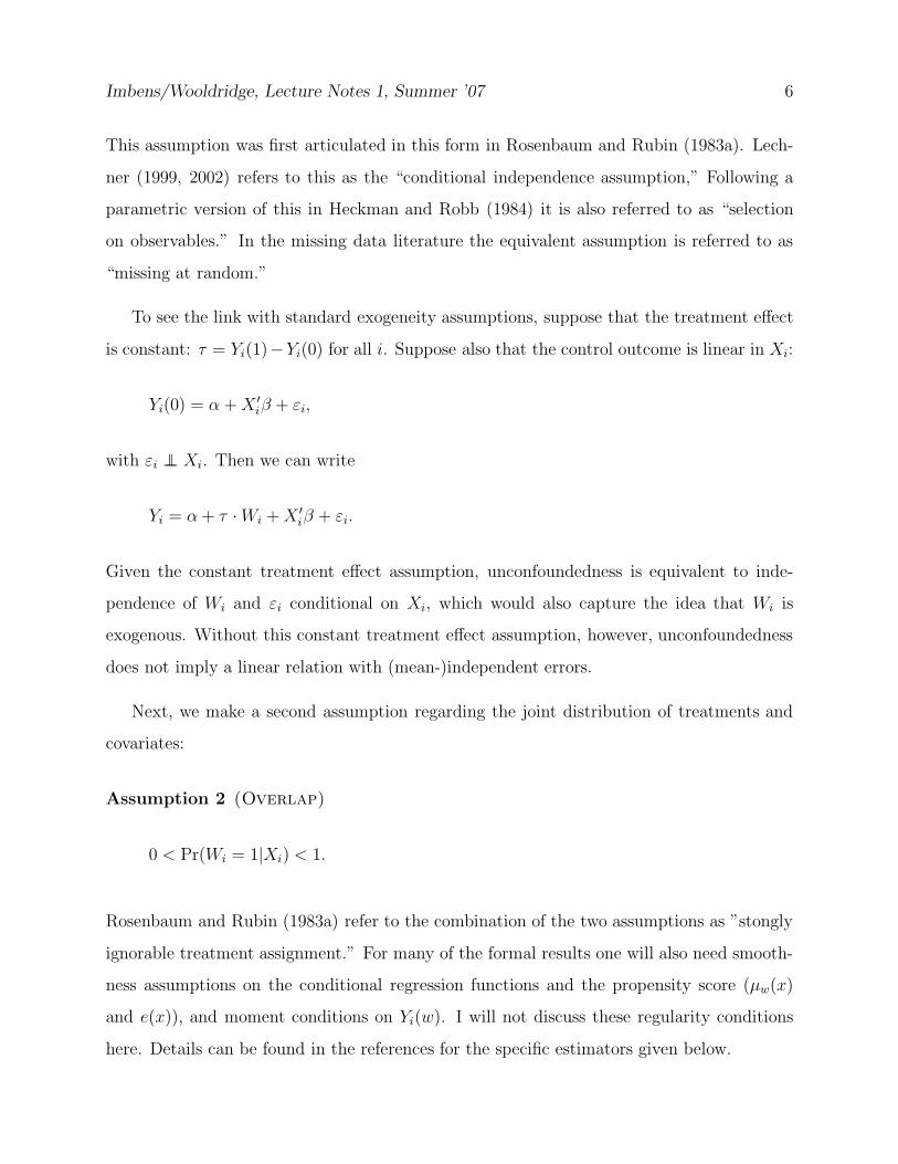
This assumption was first articulated in this form in Rosenbaum and Rubin (1983a). Lech-
ner (1999, 2002) refers to this as the “conditional independence assumption,” Following a
parametric version of this in Heckman and Robb (1984) it is also referred to as “selection
on observables.” In the missing data literature the equivalent assumption is referred to as
“missing at random.”
To see the link with standard exogeneity assumptions, suppose that the treatment effect
is constant: τ = Yi(1)−Yi(0) for all i. Suppose also that the control outcome is linear in Xi:
Yi(0) = α +X ′iβ + εi,
with εi ⊥⊥ Xi. Then we can write
Yi = α+ τ ·Wi +X ′iβ + εi.
Given the constant treatment effect assumption, unconfoundedness is equivalent to inde-
pendence of Wi and εi conditional on Xi, which would also capture the idea that Wi is
exogenous. Without this constant treatment effect assumption, however, unconfoundedness
does not imply a linear relation with (mean-)independent errors.
Next, we make a second assumption regarding the joint distribution of treatments and
covariates:
Assumption 2 (Overlap)
0 < Pr(Wi = 1|Xi) < 1.
Rosenbaum and Rubin (1983a) refer to the combination of the two assumptions as ”stongly
ignorable treatment assignment.” For many of the formal results one will also need smooth-
ness assumptions on the conditional regression functions and the propensity score (µw(x)
and e(x)), and moment conditions on Yi(w). I will not discuss these regularity conditions
here. Details can be found in the references for the specific estimators given below.

Imbens/Wooldridge, Lecture Notes 1, Summer ’07 7
There has been some controversy about the plausibility of Assumptions 1 and 2 in eco-
nomic settings and thus the relevance of the econometric literature that focuses on estimation
and inference under these conditions for empirical work. In this debate it has been argued
that agents’ optimizing behavior precludes their choices being independent of the potential
outcomes, whether or not conditional on covariates. This seems an unduly narrow view.
In response I will offer three arguments for considering these assumptions. The first is a
statistical, data descriptive motivation. A natural starting point in the evaluation of any
program is a comparison of average outcomes for treated and control units. A logical next
step is to adjust any difference in average outcomes for differences in exogenous background
characteristics (exogenous in the sense of not being affected by the treatment). Such an
analysis may not lead to the final word on the efficacy of the treatment, but the absence of
such an analysis would seem difficult to rationalize in a serious attempt to understand the
evidence regarding the effect of the treatment.
A second argument is that almost any evaluation of a treatment involves comparisons
of units who received the treatment with units who did not. The question is typically not
whether such a comparison should be made, but rather which units should be compared, that
is, which units best represent the treated units had they not been treated. Economic theory
can help in classifying variables into those that need to be adjusted for versus those that do
not, on the basis of their role in the decision process (e.g., whether they enter the utility
function or the constraints). Given that, the unconfoundedness assumption merely asserts
that all variables that need to be adjusted for are observed by the researcher. This is an
empirical question, and not one that should be controversial as a general principle. It is clear
that settings where some of these covariates are not observed will require strong assumptions
to allow for identification. Such assumptions include instrumental variables settings where
some covariates are assumed to be independent of the potential outcomes. Absent those
assumptions, typically only bounds can be identified (e.g., Manski, 1990, 1995).
A third, related, argument is that even when agents optimally choose their treatment, two
agents with the same values for observed characteristics may differ in their treatment choices
Imbens/Wooldridge, Lecture Notes 1, Summer ’07 8
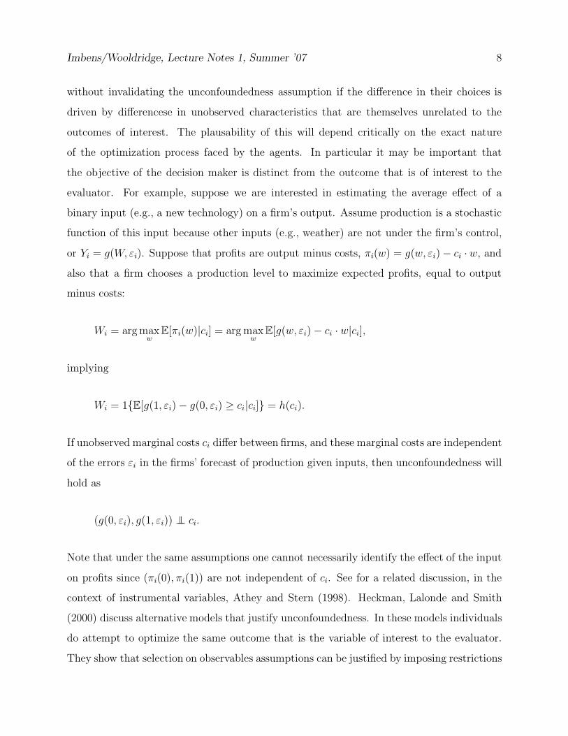
without invalidating the unconfoundedness assumption if the difference in their choices is
driven by differencese in unobserved characteristics that are themselves unrelated to the
outcomes of interest. The plausability of this will depend critically on the exact nature
of the optimization process faced by the agents. In particular it may be important that
the objective of the decision maker is distinct from the outcome that is of interest to the
evaluator. For example, suppose we are interested in estimating the average effect of a
binary input (e.g., a new technology) on a firm’s output. Assume production is a stochastic
function of this input because other inputs (e.g., weather) are not under the firm’s control,
or Yi = g(W, εi). Suppose that profits are output minus costs, πi(w) = g(w, εi) − ci ·w, and
also that a firm chooses a production level to maximize expected profits, equal to output
minus costs:
Wi = arg maxw
E[πi(w)|ci] = arg maxw
E[g(w, εi) − ci · w|ci],
implying
Wi = 1E[g(1, εi) − g(0, εi) ≥ ci|ci] = h(ci).
If unobserved marginal costs ci differ between firms, and these marginal costs are independent
of the errors εi in the firms’ forecast of production given inputs, then unconfoundedness will
hold as
(g(0, εi), g(1, εi)) ⊥⊥ ci.
Note that under the same assumptions one cannot necessarily identify the effect of the input
on profits since (πi(0), πi(1)) are not independent of ci. See for a related discussion, in the
context of instrumental variables, Athey and Stern (1998). Heckman, Lalonde and Smith
(2000) discuss alternative models that justify unconfoundedness. In these models individuals
do attempt to optimize the same outcome that is the variable of interest to the evaluator.
They show that selection on observables assumptions can be justified by imposing restrictions
Imbens/Wooldridge, Lecture Notes 1, Summer ’07 9
on the way individuals form their expectations about the unknown potential outcomes. In
general, therefore, a researcher may wish to, either as a final analysis or as part of a larger
investigation, consider estimates based on the unconfoundedness assumption.
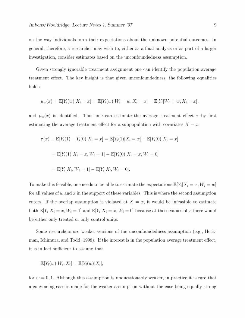
Given strongly ignorable treatment assignment one can identify the population average
treatment effect. The key insight is that given unconfoundedness, the following equalities
holds:
µw(x) = E[Yi(w)|Xi = x] = E[Yi(w)|Wi = w,Xi = x] = E[Yi|Wi = w,Xi = x],
and µw(x) is identified. Thus one can estimate the average treatment effect τ by first
estimating the average treatment effect for a subpopulation with covariates X = x:
τ (x) ≡ E[Yi(1) − Yi(0)|Xi = x] = E[Yi(1)|Xi = x] − E[Yi(0)|Xi = x]
= E[Yi(1)|Xi = x,Wi = 1] − E[Yi(0)|Xi = x,Wi = 0]
= E[Yi|Xi,Wi = 1] − E[Yi|Xi,Wi = 0].
To make this feasible, one needs to be able to estimate the expectations E[Yi|Xi = x,Wi = w]
for all values of w and x in the support of these variables. This is where the second assumption
enters. If the overlap assumption is violated at X = x, it would be infeasible to estimate
both E[Yi|Xi = x,Wi = 1] and E[Yi|Xi = x,Wi = 0] because at those values of x there would
be either only treated or only control units.
Some researchers use weaker versions of the unconfoundedness assumption (e.g., Heck-
man, Ichimura, and Todd, 1998). If the interest is in the population average treatment effect,
it is in fact sufficient to assume that
E[Yi(w)|Wi, Xi] = E[Yi(w)|Xi],
for w = 0, 1. Although this assumption is unquestionably weaker, in practice it is rare that
a convincing case is made for the weaker assumption without the case being equally strong
Imbens/Wooldridge, Lecture Notes 1, Summer ’07 10
for the stronger Assumption 1. The reason is that the weaker assumption is intrinsically
tied to functional form assumptions, and as a result one cannot identify average effects on
transformations of the original outcome (e.g., logarithms) without the strong assumption.
One can weaken the unconfoundedness assumption in a different direction if one is only
interested in the average effect for the treated (e.g., Heckman, Ichimura and Todd, 1997).
In that case one need only assume Yi(0) ⊥⊥ Wi
∣
∣
∣Xi. and the weaker overlap assumption
Pr(Wi = 1|Xi) < 1. These two assumptions are sufficient for identification of PATT because
moments of the distribution of Y (1) for the treated are directly estimable.
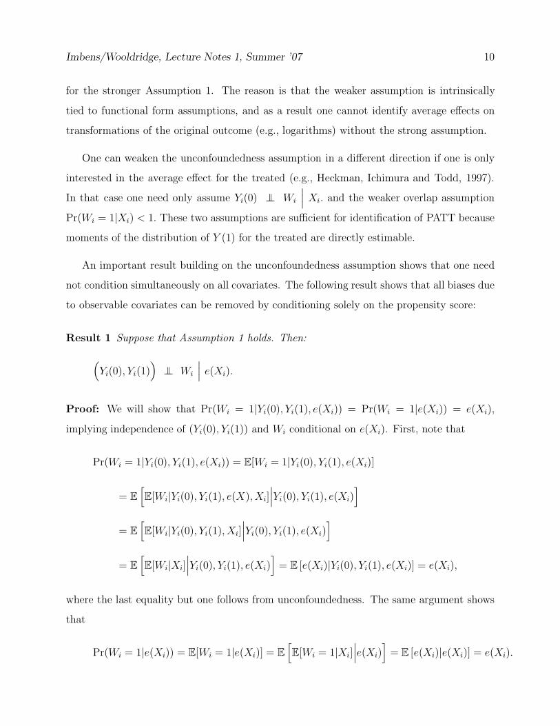
An important result building on the unconfoundedness assumption shows that one need
not condition simultaneously on all covariates. The following result shows that all biases due
to observable covariates can be removed by conditioning solely on the propensity score:
Result 1 Suppose that Assumption 1 holds. Then:
(
Yi(0), Yi(1))
⊥⊥ Wi
∣
∣
∣e(Xi).
Proof: We will show that Pr(Wi = 1|Yi(0), Yi(1), e(Xi)) = Pr(Wi = 1|e(Xi)) = e(Xi),
implying independence of (Yi(0), Yi(1)) and Wi conditional on e(Xi). First, note that
Pr(Wi = 1|Yi(0), Yi(1), e(Xi)) = E[Wi = 1|Yi(0), Yi(1), e(Xi)]
= E
[
E[Wi|Yi(0), Yi(1), e(X), Xi]∣
∣
∣Yi(0), Yi(1), e(Xi)
]
= E
[
E[Wi|Yi(0), Yi(1), Xi]∣
∣
∣Yi(0), Yi(1), e(Xi)
]
= E
[
E[Wi|Xi]∣
∣
∣Yi(0), Yi(1), e(Xi)
]
= E [e(Xi)|Yi(0), Yi(1), e(Xi)] = e(Xi),
where the last equality but one follows from unconfoundedness. The same argument shows
that
Pr(Wi = 1|e(Xi)) = E[Wi = 1|e(Xi)] = E
[
E[Wi = 1|Xi]∣
∣
∣e(Xi)
]
= E [e(Xi)|e(Xi)] = e(Xi).
Imbens/Wooldridge, Lecture Notes 1, Summer ’07 11
Extensions of this result to the multivalued treatment case are given in Imbens (2000)
and Lechner (2001).
To provide intuition for the Rosenbaum-Rubin result, recall the textbook formula for
omitted variable bias in the linear regression model. Suppose we have a regression model
with two regressors:
Yi = β0 + β1 ·Wi + β ′2Xi + εi.
The bias of omittingXi from the regression on the coefficient on Wi is equal to β ′2δ, where δ is
the vector of coefficients on Wi in regressions of the elements of Xi on Wi. By conditioning on
the propensity score we remove the correlation between Xi and Wi because Xi ⊥⊥Wi|e(Xi).
Hence omitting Xi no longer leads to any bias (although it may still lead to some efficiency
loss).
2.4 Efficiency Bounds and Asymptotic Variances for Population Average
Treatment Effects
Next we review some results on the effiency bound for estimators of the average treat-
ment effects τP . This requires strong ignorability and some smoothness assumptions on the
conditional expectations of potential outcomes and the treatment indicator (for details, see
Hahn, 1998). Formally, Hahn (1998) shows that for any regular estimator for τP , denoted
by τ , with
√N · (τ − τP )
d−→ N (0, V ),
we can show that
V ≥ E
[
σ21(Xi)
e(Xi)+
σ20(Xi)
1 − e(Xi)+ (τ (Xi) − τP )2
]
. (1)
Knowing the propensity score does not affect this efficiency bound.
Imbens/Wooldridge, Lecture Notes 1, Summer ’07 12
Hahn also shows that asymptotically linear estimators exist that achieve the efficiency
bound, and hence such efficient estimators can be approximated as
τ = τP +1
N
N∑
i=1
ψ(Yi,Wi, Xi, τP ) + op(N−1/2),
where ψ(·) is the efficient score:
ψ(y, w, x, τP) =
(
wy
e(x)− (1 − w)y
1 − e(x)
)
− τP −(
µ1(x)
e(x)+
µ0(x)
1 − e(x)
)
· (w − e(x)). (2)
3. Estimating Average Treatment Effects
Here we discuss the leading estimators for average treatment effects under unconfounded-
ness. What is remarkable about this literature is the wide range of ostensibly quite different
estimators, many of which are regularly used in empirical work. We first briefly describe a
number of the estimators, and then discuss their relative merits.
3.1 Regression
The first class of estimators relies on consistent estimation of µw(x) for w = 0, 1. Given
µw(x) for these regression functions, the PATE and SATE are estimated by averaging their
difference over the empirical distribution of the covariates:
τreg =1
N
N∑
i=1
(
µ1(Xi) − µ0(Xi))
. (3)
In most implementations the average of the predicted treated outcome for the treated is
equal to the average observed outcome for the treated (so that∑
i Wi · µ1(Xi) =∑
iWi ·Yi),
and similarly for the controls, implying that τreg can also be written as
τreg =1
N
N∑
i=1
Wi ·(
Yi − µ0(Xi))
+ (1 −Wi) ·(
µ1(Xi) − Yi
)
.
Early estimators for µw(x) included parametric regression functions, for example linear re-
gression (e.g., Rubin, 1977). Such parametric alternatives include least squares estimators
Imbens/Wooldridge, Lecture Notes 1, Summer ’07 13
with the regression function specified as
µw(x) = β ′x+ τ · w,
in which case the average treatment effect is equal to τ . In this case one can estimate τ
simply by least squares estimation using the regression function
Yi = α+ β ′Xi + τ ·Wi + εi.
More generally, one can specify separate regression functions for the two regimes, µw(x) =
β ′wx. In that case one estimate the two regression functions separately on the two subsamples
and then substitute the predicted values in (3).
These simple regression estimators can be sensitive to differences in the covariate dis-
tributions for treated and control units. The reason is that in that case the regression
estimators rely heavily on extrapolation. To see this, note that the regression function for
the controls, µ0(x) is used to predict missing outcomes for the treated. Hence on average
one wishes to use predict the control outcome at XT =∑
iWi · Xi/NT , the average covari-
ate value for the treated. With a linear regression function, the average prediction can be
written as YC + β ′(XT − XC). If XT and the average covariate value for the controls, XC
are close, the precise specification of the regression function will not matter much for the
average prediction. However, with the two averages very different, the prediction based on
a linear regression function can be sensitive to changes in the specification.
More recently, nonparametric estimators have been proposed. Imbens, Newey and Ridder
(2005) and Chen, Hong, and Tarozzi (2005) propose estimating µw(x) through series or sieve
methods. A simple version of that with a scalar X would specify the regression function as
µw(x) =
LN∑
l=0
βw,l · xk,
with LN , the number of terms in the polynomial expansion, an increasing function of the
sample size. They show that this estimator for τP achieves the semiparametric efficiency
Imbens/Wooldridge, Lecture Notes 1, Summer ’07 14
bounds. Heckman, Ichimura and Todd (1997, 1998), and Heckman, Ichimura, Smith and
Todd (1998) consider kernel methods for estimating µw(x), in particular focusing on local
linear approaches. Given a kernel K(·), and a bandwidth hN let
(
αw,x, βw,x
)
= arg minαw,x,βw,x
N∑
i=1
K
(
Xi − x
hN
)
· (Yi − αw,x − βw,x ·Xi)2 ,
leading to the estimator
µw(x) = αw,x.
3.2 Matching
Regression estimators impute the missing potential outcomes using the estimated regres-
sion function. Thus, if Wi = 1, Yi(1) is observed and Yi(0) is missing and imputed with a
consistent estimator µ0(Xi) for the conditional expectation. Matching estimators also im-
pute the missing potential outcomes, but do so using only the outcomes of nearest neighbours
of the opposite treatment group. In that sense matching is similar to nonparametric kernel
regression methods, with the number of neighbors playing the role of the bandwidth in the
kernel regression. In fact, matching can be inrrepreted as a limiting version of the standard
kernel estimator where the bandwidth goes to zero. This minimizes the bias among nonneg-
ative kernels, but potentially increases the variance relative to kernel estimators. A formal
difference with kernel estimators is that the asymptotic distribution is derived conditional on
the implicit bandwidth, that is, the number of neighbours, which is often fixed at one. Using
such asymptotics, the implicit estimate µw(x) is (close to) unbiased, but not consistent for
µw(x). In contrast, the regression estimators discussed earlier relied on the consistency of
µw(x).
Matching estimators have the attractive feature that given the matching metric, the re-
searcher only has to choose the number of matches. In contrast, for the regression estimators
discussed above, the researcher must choose smoothing parameters that are more difficult
to interpret; either the number of terms in a series or the bandwidth in kernel regression.
Imbens/Wooldridge, Lecture Notes 1, Summer ’07 15
Within the class of matching estimators, using only a single match leads to the most credible
inference with the least bias, at most sacrificing some precision. This can make the matching
estimator easier to use than those estimators that require more complex choices of smoothing
parameters, and may explain some of its popularity.
Matching estimators have been widely studied in practice and theory (e.g., Gu and Rosen-
baum, 1993; Rosenbaum, 1989, 1995, 2002; Rubin, 1973b, 1979; Heckman, Ichimura and
Todd, 1998; Dehejia and Wahba, 1999; Abadie and Imbens, 2002, AI). Most often they
have been applied in settings with the following two characteristics: (i) the interest is in
the average treatment effect for the treated, and (ii), there is a large reservoir of potential
controls. This allows the researcher to match each treated unit to one or more distinct con-
trols (referred to as matching without replacement). Given the matched pairs, the treatment
effect within a pair is then estimated as the difference in outcomes, with an estimator for the
PATT obtained by averaging these within-pair differences. Since the estimator is essentially
the difference in two sample means, the variance is calculated using standard methods for
differences in means or methods for paired randomized experiments. The remaining bias is
typically ignored in these studies. The literature has studied fast algorithms for matching
the units, as fully efficient matching methods are computationally cumbersome (e.g., Gu
and Rosenbaum, 1993; Rosenbaum, 1995). Note that in such matching schemes the order in
which the units are matched is potentially important.
Here we focus on matching estimators for PATE and SATE. In order to estimate these
targes we need to match both treated and controls, and allow for matching with replacement.
Formally, given a sample, (Yi, Xi,Wi)Ni=1, let `m(i) be the index l that satisfies Wl 6= Wi
and
∑
j|Wj 6=Wi
1
‖Xj −Xi‖ ≤ ‖Xl −Xi‖
= m,
where 1· is the indicator function, equal to one if the expression in brackets is true and
zero otherwise. In other words, `m(i) is the index of the unit in the opposite treatment group
that is the m-th closest to unit i in terms of the distance measure based on the norm ‖ · ‖.
Imbens/Wooldridge, Lecture Notes 1, Summer ’07 16
In particular, `1(i) is the nearest match for unit i. Let JM(i) denote the set of indices for
the first M matches for unit i: JM(i) = `1(i), . . . , `M (i). Define the imputed potential
outcomes as:
Yi(0) =
Yi if Wi = 0,1M
∑
j∈JM(i) Yj if Wi = 1,Yi(1) =
1M
∑
j∈JM(i) Yj if Wi = 0,
Yi if Wi = 1.
The simple matching estimator is then
τ smM =
1
N
N∑
i=1
(
Yi(1) − Yi(0))
. (4)
AI show that the bias of this estimator is of order O(N−1/K), where K is the dimension
of the covariates. Hence, if one studies the asymptotic distribution of the estimator by
normalizing by√N (as can be justified by the fact that the variance of the estimator is of
order O(1/N)), the bias does not disappear if the dimension of the covariates is equal to
two, and will dominate the large sample variance if K is at least three.
Let us make clear three caveats to the AI result. First, it is only the continuous covariates
that should be counted in K. With discrete covariates the matching will be exact in large
samples, therefore such covariates do not contribute to the order of the bias. Second, if
one matches only the treated, and the number of potential controls is much larger than the
number of treated units, one can justify ignoring the bias by appealling to an asymptotic
sequence where the number of potential controls increases faster than the number of treated
units. Specifically, if the number of controls, N0, and the number of treated, N1, satisfy
N1/N4/K0 → 0, then the bias disappears in large samples after normalization by
√N 1.
Third, even though the order of the bias may be high, the actual bias may still be small
if the coefficients in the leading term are small. This is possible if the biases for different
units are at least partially offsetting. For example, the leading term in the bias relies on the
regression function being nonlinear, and the density of the covariates having a nonzero slope.
If either the regression function is close to linear, or the density of the covariates close to
constant, the resulting bias may be fairly limited. To remove the bias, AI suggest combining
the matching process with a regression adjustment.
Imbens/Wooldridge, Lecture Notes 1, Summer ’07 17
Another point made by AI is that matching estimators are generally not efficient. Even
in the case where the bias is of low enough order to be dominated by the variance, the
estimators are not efficient given a fixed number of matches. To reach efficiency one would
need to increase the number of matches with the sample size, as done implicitly in kernel
estimators. In practice the efficiency loss is limited though, with the gain of going from two
matches to a large number of matches bounded as a fraction of the standard error by 0.16
(see AI).
In the above discussion the distance metric in choosing the optimal matches was the
standard Euclidan metric dE(x, z) = (x − z)′(x − z). All of the distance metrics used in
practice standardize the covariates in some manner. The most popular metrics are the
Mahalanobis metric, where
dM (x, z) = (x− z)′(Σ−1X )(x− z),
where Σ is covariance matrix of the covairates, and the diagonal version of that
dAI(x, z) = (x− z)′diag(Σ−1X )(x− z).
Note that depending on the correlation structure, using the Mahalanobis metric can lead to
situations where a unit with Xi = (5, 5) is a closer match for a unith with Xi = (0, 0) than
a unit with Xi = (1, 4), despite being further away in terms of each covariate separately.
3.3 Propensity Score Methods
Since the work by Rosenbaum and Rubin (1983a) there has been considerable interest in
methods that avoid adjusting directly for all covariates, and instead focus on adjusting for
differences in the propensity score, the conditional probability of receiving the treatment.
This can be implemented in a number of different ways. One can weight the observations
in terms of the propensity score (and indirectly also in terms of the covariates) to create
balance between treated and control units in the weighted sample. Hirano, Imbens and
Ridder (2003) show how such estimators can achieve the semiparametric efficiency bound.
Imbens/Wooldridge, Lecture Notes 1, Summer ’07 18
Alternatively one can divide the sample into subsamples with approximately the same value
of the propensity score, a technique known as blocking. Finally, one can directly use the
propensity score as a regressor in a regression approach or match on the propensity score.
If the researcher knows the propensity score all three of these methods are likely to be
effective in eliminating bias. Even if the resulting estimator is not fully efficient, one can
easily modify it by using a parametric estimate of the propensity score to capture most of
the efficiency loss. Furthermore, since these estimators do not rely on high-dimensional non-
parametric regression, this suggests that their finite sample properties would be attractive.
In practice the propensity score is rarely known, and in that case the advantages of
the estimators discussed below are less clear. Although they avoid the high-dimensional
nonparametric estimation of the two conditional expectations µw(x), they require instead
the equally high-dimensional nonparametric estimation of the propensity score. In practice
the relative merits of these estimators will depend on whether the propensity score is more
or less smooth than the regression functions, or whether additional information is available
about either the propensity score or the regression functions.
3.3.1 Weighting
The first set of “propensity score” estimators use the propensity score as weights to
create a balanced sample of treated and control observations. Simply taking the difference
in average outcomes for treated and controls,
τ =
∑
WiYi∑
Wi−
∑
(1 −Wi)Yi∑
1 −Wi,
is not unbiased for τP = E[Yi(1)−Yi(0)] because, conditional on the treatment indicator, the
distributions of the covariates differ. By weighting the units by the inverse of the probability
of receiving the treatment, one can undo this imbalance. Formally, weighting estimators rely
on the equalities:
E
[
WY
e(X)
]
= E
[
WYi(1)
e(X)
]
= E
[
E
[
WYi(1)
e(X)
∣
∣
∣
∣
X
]]
= E
[
E
[
e(X)Yi(1)
e(X)
]]
= E[Yi(1)],
Imbens/Wooldridge, Lecture Notes 1, Summer ’07 19
and similarly
E
[
(1 −W )Y
1 − e(X)
]
= E[Yi(0)],
implying
τP = E
[
W · Ye(X)
− (1 −W ) · Y1 − e(X)
]
.
With the propensity score known one can directly implement this estimator as
τ =1
N
N∑
i=1
(
WiYi
e(Xi)− (1 −Wi)Yi
1 − e(Xi)
)
. (5)
In this particular form this is not necessarily an attractive estimator. The main reason is
that, although the estimator can be written as the difference between a weighted average of
the outcomes for the treated units and a weighted average of the outcomes for the controls,
the weights do not necessarily add to one. Specifically, in (5), the weights for the treated
units add up to (∑
Wi/e(Xi))/N . In expectation this is equal to one, but since its variance
is positive, in any given sample some of the weights are likely to deviate from one. One
approach for improving this estimator is simply to normalize the weights to unity. One can
further normalize the weights to unity within subpopulations as defined by the covariates.
In the limit this leads to the estimator proposed by Hirano, Imbens and Ridder (2003) who
suggest using a nonparametric series estimator for e(x). More precisely, they first specify a
sequence of functions of the covariates, e.g., a power series, hl(x), l = 1, . . . ,∞. Next, they
choose a number of terms, L(N), as a function of the sample size, and then estimate the
L-dimensional vector γL in
Pr(W = 1|X = x) =exp((h1(x), . . . , hL(x))γL)
1 + exp((h1(x), . . . , hL(x))γL),
by maximizing the associated likelihood function. Let γL be the maximum likelihood esti-
mate. In the third step, the estimated propensity score is calculated as:
e(x) =exp((h1(x), . . . , hL(x))γL)
1 + exp((h1(x), . . . , hL(x))γL).

Imbens/Wooldridge, Lecture Notes 1, Summer ’07 20
Finally they estimate the average treatment effect as:
τweight =N
∑
i=1
Wi · Yi
e(Xi)
/
N∑
i=1
Wi
e(Xi)−
N∑
i=1
(1 −Wi) · Yi
1 − e(Xi)
/
N∑
i=1
(1 −Wi)
1 − e(Xi). (6)
Hirano, Imbens and Ridder (2003) show that this estimator is efficient, whereas with the true
propensity score the estimator would not be fully efficient (and in fact not very attractive).
This estimator highlights one of the interesting features of the problem of efficiently es-
timating average treatment effects. One solution is to estimate the two regression functions
µw(x) nonparametrically; that solution completely ignores the propensity score. A second
approach is to estimate the propensity score nonparametrically, ignoring entirely the two
regression functions. If appropriately implemented, both approaches lead to fully efficient
estimators, but clearly their finite sample properties may be very different, depending, for
example, on the smoothness of the regression functions versus the smoothness of the propen-
sity score. If there is only a single binary covariate, or more generally with only discrete
covariates, the weighting approach with a fully nonparametric estimator for the propensity
score is numerically identical to the regression approach with a fully nonparametric estimator
for the two regression functions.
One difficulty with the weighting estimators that are based on the estimated propensity
score is again the problem of choosing the smoothing parameters. Hirano, Imbens and Rid-
der (2003) use series estimators, which requires choosing the number of terms in the series.
Ichimura and Linton (2001) consider a kernel version, which involves choosing a bandwidth.
Theirs is currently one of the few studies considering optimal choices for smoothing param-
eters that focuses specifically on estimating average treatment effects. A departure from
standard problems in choosing smoothing parameters is that here one wants to use non-
parametric regression methods even if the propensity score is known. For example, if the
probability of treatment is constant, standard optimality results would suggest using a high
degree of smoothing, as this would lead to the most accurate estimator for the propensity
score. However, this would not necessarily lead to an efficient estimator for the average
treatment effect of interest.
Imbens/Wooldridge, Lecture Notes 1, Summer ’07 21
3.3.2 Blocking on the Propensity Score
In their original propensity score paper Rosenbaum and Rubin (1983a) suggest the fol-
lowing “blocking propensity score” estimator. Using the (estimated) propensity score, divide
the sample into M blocks of units of approximately equal probability of treatment, letting
Jim be an indicator for unit i being in block m. One way of implementing this is by dividing
the unit interval into M blocks with boundary values equal to m/M for m = 1, . . . ,M − 1,
so that
Jim = 1(m− 1)/M < e(Xi) ≤ m/M,
for m = 1, . . . ,M . Within each block there are Nwm observations with treatment equal to
w, Nwm =∑
i 1Wi = w, Jim = 1. Given these subgroups, estimate within each block the
average treatment effect as if random assignment holds,
τm =1
N1m
N∑
i=1
JimWiYi −1
N0m
N∑
i=1
Jim(1 −Wi)Yi.
Then estimate the overall average treatment effect as:
τblock =M
∑
m=1
τm · N1m +N0m
N.
Blocking can be interpreted as a crude form of nonparametric regression where the un-
known function is approximated by a step function with fixed jump points. To establish
asymptotic properties for this estimator would require establishing conditions on the rate
at which the number of blocks increases with the sample size. With the propensity score
known, these are easy to determine; no formal results have been established for the unknown
case.
The question arises how many blocks to use in practice. Cochran (1968) analyses a case
with a single covariate, and, assuming normality, shows that using five blocks removes at least
95% of the bias associated with that covariate. Since all bias, under unconfoudnedness, is

Imbens/Wooldridge, Lecture Notes 1, Summer ’07 22
associated with the propensity score, this suggests that under normality five blocks removes
most of the bias associated with all the covariates. This has often been the starting point
of empirical analyses using this estimator (e.g., Rosenbaum and Rubin, 1983b; Dehejia
and Wahba, 1999), and has been implemented in STATA by Becker and Ichino (2002).
Often, however, researchers subsequently check the balance of the covariates within each
block. If the true propensity score per block is constant, the distribution of the covariates
among the treated and controls should be identical, or, in the evaluation terminology, the
covariates should be balanced. Hence one can assess the adequacy of the statistical model
by comparing the distribution of the covariates among treated and controls within blocks.
If the distributions are found to be different, one can either split the blocks into a number
of subblocks, or generalize the specification of the propensity score. Often some informal
version of the following algorithm is used: If within a block the propensity score itself is
unbalanced, the blocks are too large and need to be split. If, conditional on the propensity
score being balanced, the covariates are unbalanced, the specification of the propensity score
is not adequate. No formal algorithm exists for implementing these blocking methods.
3.3.3 Regression on the Propensity Score
The third method of using the propensity score is to estimate the conditional expectation
of Y given W and e(X) and average the difference. Although this method has been used
in practice, there is no particular reason why this is an attractive method compared to the
regression methods based on the covariates directly. In addition, the large sample properties
have not been established.
3.3.4 Matching on the Propensity Score
The Rosenbaum-Rubin result implies that it is sufficient to adjust solely for differences in
the propensity score between treated and control units. Since one of the ways in which one
can adjust for differences in covariates is matching, another natural way to use the propensity
score is through matching. Because the propensity score is a scalar function of the covariates,
the bias results in Abadie and Imbens (2002) imply that the bias term is of lower order
Imbens/Wooldridge, Lecture Notes 1, Summer ’07 23
than the variance term and matching leads to a√N -consistent, asymptotically normally
distributed estimator. The variance for the case with matching on the true propensity score
also follows directly from their results. More complicated is the case with matching on
the estimated propensity score. We are not aware of any results that give the asymptotic
variance for this case.
3.4. Mixed Methods
A number of approaches have been proposed that combine two of the three methods de-
scribed earlier, typically regression with one of its alternatives. These methods appear to be
the most attractive in practice. The motivation for these combinations is that, although one
method alone is often sufficient to obtain consistent or even efficient estimates, incorporating
regression may eliminate remaining bias and improve precision. This is particularly useful
because neither matching nor the propensity score methods directly address the correlation
between the covariates and the outcome. The benefit associated with combining methods is
made explicit in the notion developed by Robins and Ritov (1997) of “double robustness.”
They propose a combination of weighting and regression where, as long as the parametric
model for either the propensity score or the regression functions is specified correctly, the re-
sulting estimator for the average treatment effect is consistent. Similarly, because matching
is consistent with few assumptions beyond strong ignorability, thus methods that combine
matching and regressions are robust against misspecification of the regression function.
3.4.1 Weighting and Regression
One can rewrite the HIR weighting estimator discussed above as estimating the following
regression function by weighted least squares,
Yi = α+ τ ·Wi + εi,
with weights equal to
λi =
√
Wi
e(Xi)+
1 −Wi
1 − e(Xi).
Imbens/Wooldridge, Lecture Notes 1, Summer ’07 24
Without the weights the least squares estimator would not be consistent for the average
treatment effect; the weights ensure that the covariates are uncorrelated with the treatment
indicator and hence the weighted estimator is consistent.
This weighted-least-squares representation suggests that one may add covariates to the
regression function to improve precision, for example as
Yi = α+ β ′Xi + τ ·Wi + εi,
with the same weights λi. Such an estimator, using a more general semiparametric regression
model, is suggested in Robins and Rotnitzky (1995), Robins, Rotnitzky and Zhao (1995),
Robins and Ritov (1997), and implemented in Hirano and Imbens (2001). In the parametric
context Robins and Ritov argue that the estimator is consistent as long as either the regres-
sion model or the propensity score (and thus the weights) are specified correctly. That is, in
the Robins-Ritov terminology, the estimator is doubly robust.
3.4.2 Blocking and Regression
Rosenbaum and Rubin (1983b) suggest modifying the basic blocking estimator by using
least squares regression within the blocks. Without the additional regression adjustment the
estimated treatment effect within blocks can be written as a least squares estimator of τm
for the regression function
Yi = αm + τm ·Wi + εi,
using only the units in block m. As above, one can also add covariates to the regression
function
Yi = αm + τm ·Wi + β ′mXi + εi,
again estimated on the units in block m.
3.4.3 Matching and Regression
Imbens/Wooldridge, Lecture Notes 1, Summer ’07 25
Since Abadie and Imbens (2002) show that the bias of the simple matching estimator
can dominate the variance if the dimension of the covariates is too large, additional bias
corrections through regression can be particularly relevant in this case. A number of such
corrections have been proposed, first by Rubin (1973b) and Quade (1982) in a parametric
setting. Let Yi(0) and Yi(1) be the observed or imputed potential outcomes for unit i; where
these estimated potential outcomes equal observed outcomes for some unit i and its match
`(i). The bias in their comparison, E[Yi(1) − Yi(0)] − (Yi(1) − Yi(0)), arises from the fact
that the covariates for units i and `(i), Xi and X`(i) are not equal, although close because
of the matching process.
To further explore this, focusing on the single match case, define for each unit:
Xi(0) =
Xi if Wi = 0,X`(i) if Wi = 1,
Xi(1) =
X`(i) if Wi = 0,Xi if Wi = 1.
If the matching is exact Xi(0) = Xi(1) for each unit. If not, these discrepancies will lead to
potential bias. The difference Xi(1) − Xi(0) will therefore be used to reduce the bias of the
simple matching estimator.
Suppose unit i is a treated unit (Wi = 1), so that Yi(1) = Yi(1) and Yi(0) is an imputed
value for Yi(0). This imputed value is unbiased for µ0(X`(i)) (since Yi(0) = Y`(i)), but not
necessarily for µ0(Xi). One may therefore wish to adjust Yi(0) by an estimate of µ0(Xi) −µ0(X`(i)). Typically these corrections are taken to be linear in the difference in the covariates
for units i and its match, that is, of the form β ′0(Xi(1)−Xi(0) = β ′
0(Xi−X`(i)). One proposed
correction is to estimate µ0(x) directly by taking the control units that are used as matches for
the treated units, with weights corresponding to the number of times a control observations
is used as a match, and estimate a linear regression of the form
Yi = α0 + β ′0Xi + εi,
on the weighted control observations by least squares. (If unit i is a control unit the correc-
tion would be done using an estimator for the regression function µ1(x) based on a linear
Imbens/Wooldridge, Lecture Notes 1, Summer ’07 26
specification Yi = α1 + β ′1Xi estimated on the treated units.) AI show that if this correction
is done nonparametrically, the resulting matching estimator is consistent and asymptotically
normal, with its bias dominated by the variance.
4. Estimating Variances
The variances of the estimators considered so far typically involve unknown functions.
For example, as discussed earlier, the variance of efficient estimators of PATE is equal to
VP = E
[
σ21(Xi)
e(Xi)+
σ20(Xi)
1 − e(Xi)+ (µ1(Xi) − µ0(Xi) − τ )2
]
,
involving the two regression functions, the two conditional variances and the propensity
score.
4.1 Estimating The Variance of Efficient Estimators for τP
For efficient estimators for τP the asymptotic variance is equal to the efficiency bound
VP . There are a number of ways we can estimate this. The first is essentially by brute force.
All five components of the variance, σ20(x), σ
21(x), µ0(x), µ1(x), and e(x), are consistently
estimable using kernel methods or series, and hence the asymptotic variance can be estimated
consistently. However, if one estimates the average treatment effect using only the two
regression functions, it is an additional burden to estimate the conditional variances and
the propensity score in order to estimate VP . Similarly, if one efficiently estimates the
average treatment effect by weighting with the estimated propensity score, it is a considerable
additional burden to estimate the first two moments of the conditional outcome distributions
just to estimate the asymptotic variance.
A second method applies to the case where either the regression functions or the propen-
sity score is estimated using series or sieves. In that case one can interpret the estimators,
given the number of terms in the series, as parametric estimators, and calculate the vari-
ance this way. Under some conditions that will lead to valid standard errors and confidence
intervals.
Imbens/Wooldridge, Lecture Notes 1, Summer ’07 27
A third approach is to use bootstrapping (Efron and Tibshirani, 1993; Horowitz, 2002).
Although there is little formal evidence specific for these estimators, given that the estimators
are asymptotically linear, it is likely that bootstrapping will lead to valid standard errors and
confidence intervals at least for the regression and propensity score methods. Bootstrapping
is not valid for matching estimators, as shown by Abadie and Imbens (2007) Subsampling
(Politis and Romano, 1999) will still work in this setting.
4.2 Estimating The Conditional Variance
Here we focus on estimation of the variance of estimators for τS , which is the condi-
tional variance of the various estimators, conditional on the covariates X and the treatment
indicators W. All estimators used in practice are linear combinations of the outcomes,
τ =
N∑
i=1
λi(X,W) · Yi,
with the λ(X,W) known functions of the covariates and treatment indicators. Hence the
conditional variance is
V (τ |X,W) =N
∑
i=1
λi(X,W)2 · σ2Wi
(Xi).
The only unknown component of this variance is σ2w(x). Rather than estimating this through
nonparametric regression, AI suggest using matching to estimate σ2w(x). To estimate σ2
Wi(Xi)
one uses the closest match within the set of units with the same treatment indicator. Let
v(i) be the closest unit to i with the same treatment indicator (Wv(i) = Wi). The sample
variance of the outcome variable for these 2 units can then be used to estimate σ2Wi
(Xi):
σ2Wi
(Xi) =(
Yi − Yv(i)
)2/2.
Note that this estimator is not consistent estimators of the conditional variances. However
this is not important, as we are interested not in the variances at specific points in the
Imbens/Wooldridge, Lecture Notes 1, Summer ’07 28
covariates distribution, but in the variance of the average treatment effect. Following the
process introduce above, this is estimated as:
V (τ |X,W) =N
∑
i=1
λi(X,W)2 · σ2Wi
(Xi).
5. Assessing Unconfoundedness
The unconfoundedness assumption used throughout this discussion is not directly testable.
It states that the conditional distribution of the outcome under the control treatment, Yi(0),
given receipt of the active treatment and given covariates, is identical to the distribution of
the control outcome given receipt of the control treatment and given covariates. The same is
assumed for the distribution of the active treatment outcome, Yi(1). Yet since the data are
completely uninformative about the distribution of Yi(0) for those who received the active
treatment and of Yi(1) for those receiving the control, the data cannot directly reject the
unconfoundedness assumption. Nevertheless, there are often indirect ways of assessing the
this, a number of which are developed in Heckman and Hotz (1989) and Rosenbaum (1987).
These methods typically rely on estimating a causal effect that is known to equal zero. If
based on the test we reject the null hypothesis that this causal effect varies from zero, the
unconfoundedness assumption is considered less plausible. These tests can be divided into
two broad groups.
The first set of tests focuses on estimating the causal effect of a treatment that is known
not to have an effect, relying on the presence of multiple control groups (Rosenbaum, 1987).
Suppose one has two potential control groups, for example eligible nonparticipants and
ineligibles, as in Heckman, Ichimura and Todd (1997). One interpretation of the test is
to compare average treatment effects estimated using each of the control groups. This can
also be interpreted as estimating an “average treatment effect” using only the two control
groups, with the treatment indicator now a dummy for being a member of the first group.
In that case the treatment effect is known to be zero, and statistical evidence of a non-zero
effect implies that at least one of the control groups is invalid. Again, not rejecting the
test does not imply the unconfoundedness assumption is valid (as both control groups could
Imbens/Wooldridge, Lecture Notes 1, Summer ’07 29
suffer the same bias), but non-rejection in the case where the two control groups are likely
to have different biases makes it more plausible that the unconfoundness assumption holds.
The key for the power of this test is to have available control groups that are likely to have
different biases, if at all. Comparing ineligibles and eligible nonparticipants is a particularly
attractive comparison. Alternatively one may use different geographic controls, for example
from areas bordering on different sides of the treatment group.
One can formalize this test by postulating a three-valued indicator Ti ∈ −0, 1, 1 for the
groups (e.g., ineligibles, eligible nonnonparticipants and participants), with the treatment
indicator equal to Wi = 1Ti = 1, so that
Yi =
Yi(0) if Ti ∈ −1, 0Yi(1) if Ti = 1.
If one extends the unconfoundedness assumption to independence of the potential outcomes
and the three-valued group indicator given covariates,
Yi(0), Yi(1) ⊥⊥ Ti
∣
∣
∣
∣
Xi,
then a testable implication is
Yi(0) ⊥⊥ 1Ti = 0∣
∣
∣
∣
Xi, Ti ∈ −1, 0,
and thus
Yi ⊥⊥ 1Ti = 0∣
∣
∣
∣
Xi, Ti ∈ −1, 0.
An implication of this independence condition is being tested by the tests discussed above.
Whether this test has much bearing on the unconfoundedness assumption depends on whether
the extension of the assumption is plausible given unconfoundedness itself.
The second set of tests of unconfoundedness focuses on estimating the causal effect of
the treatment on a variable known to be unaffected by it, typically because its value is
Imbens/Wooldridge, Lecture Notes 1, Summer ’07 30
determined prior to the treatment itself. Such a variable can be time-invariant, but the
most interesting case is in considering the treatment effect on a lagged outcome, commonly
observed in labor market programs. If the estimated effect differs from zero, this implies that
the treated observations are different from the controls in terms of this particular covariate
given the others. If the treatment effect is estimated to be close to zero, it is more plausible
that the unconfoundedness assumption holds. Of course this does not directly test this
assumption; in this setting, being able to reject the null of no effect does not directly reflect
on the hypothesis of interest, unconfoundedness. Nevertheless, if the variables used in this
proxy test are closely related to the outcome of interest, the test arguably has more power.
For these tests it is clearly helpful to have a number of lagged outcomes.
To formalize this, let us suppose the covariates consist of a number of lagged out-
comes Yi,−1, . . . , Yi,−T as well as time-invariant individual characteristics Zi, so that Xi =
(Yi,−1, . . . , Yi,−T , Zi). By construction only units in the treatment group after period −1
receive the treatment; all other observed outcomes are control outcomes. Also suppose that
the two potential outcomes Yi(0) and Yi(1) correspond to outcomes in period zero. Now
consider the following two assumptions. The first is unconfoundedness given only T − 1 lags
of the outcome:
Yi,0(1), Yi,0(0) ⊥⊥ Wi
∣
∣
∣Yi,−1, . . . , Yi,−(T−1), Zi,
and the second assumes stationarity and exchangeability:
fYi,s(0)|Yi,s−1(0),...,Yi,s−(T−1)(0),Zi,Wi(ys|ys−1, . . . , ys−(T−1), z, w), does not depend on i and s.
Then it follows that
Yi,−1 ⊥⊥ Wi
∣
∣
∣Yi,−2, . . . , Yi,−T , Zi,
which is testable. This hypothesis is what the procedure described above tests. Whether
this test has much bearing on unconfoundedness depends on the link between the two as-
sumptions and the original unconfoundedness assumption. With a sufficient number of lags

Imbens/Wooldridge, Lecture Notes 1, Summer ’07 31
unconfoundedness given all lags but one appears plausible conditional on unconfoundedness
given all lags, so the relevance of the test depends largely on the plausibility of the second
assumption, stationarity and exchangeability.
6. Assessing Overlap
The second of the key assumptions in estimating average treatment effects requires that
the propensity score is strictly between zero and one. Although in principle this is testable,
as it restricts the joint distribution of observables, formal tests are not the main concern.
In practice, this assumption raises a number of issues. The first question is how to detect
a lack of overlap in the covariate distributions. A second is how to deal with it, given that
such a lack exists.
6.1 Propensity Score Distributions
The first method to detect lack of overlap is to plot distributions of covariates by treat-
ment groups. In the case with one or two covariates one can do this directly. In high
dimensional cases, however, this becomes more difficult. One can inspect pairs of marginal
distributions by treatment status, but these are not necessarily informative about lack of
overlap. It is possible that for each covariate the distribution for the treatment and control
groups are identical, even though there are areas where the propensity score is zero or one.
A more direct method is to inspect the distribution of the propensity score in both
treatment groups, which can reveal lack of overlap in the multivariate covariate distributions.
Its implementation requires nonparametric estimation of the propensity score, however, and
misspecification may lead to failure in detecting a lack of overlap, just as inspecting various
marginal distributions may be insufficient. In practice one may wish to undersmooth the
estimation of the propensity score, either by choosing a bandwidth smaller than optimal for
nonparametric estimation or by including higher order terms in a series expansion.
6.2 Selecting a Sample with Overlap
Once one determines that there is a lack of overlap one can either conclude that the
Imbens/Wooldridge, Lecture Notes 1, Summer ’07 32
average treatment effect of interest cannot be estimated with sufficient precision, and/or
decide to focus on an average treatment effect that is estimable with greater accuracy. To do
the latter it can be useful to discard some of the observations on the basis of their covariates.
For example one may decide to discard control (treated) observations with propensity scores
below (above) a cutoff level. To do this sytematically, we follow Crump, Hotz, Imbens
and Mitnik (2006), who focus on sample averate treatment effects. Their starting point is
the definition of average treatment effects for subsets of the covariate space. Let X be the
covariate space, and A ⊂ X be some subset. Then define
τ (A) =N
∑
i=1
1Xi ∈ A · τ (Xi)/
N∑
i=1
1Xi ∈ A.
Crump et al calculate the efficiency bound for τ (A), assuming homoskedasticity, as
σ2
q(A)· E
[
1
e(X)+
1)
1 − e(X)
∣
∣
∣
∣
X ∈ A
]
,
where q(A) = Pr(X ∈ A). They derive the characterization for the set A that minimizes the
asymptotic variance and show that it has the form
A∗ = x ∈ X|α ≤ e(X) ≤ 1 − α,
dropping observations with extreme values for the propensity score, with the cutoff value α
determined by the equation
1
α · (1 − α)= 2 · E
[
1
e(X) · (1 − e(X))
∣
∣
∣
∣
1
e(X) · (1 − e(X))≤ 1
α · (1 − α)
]
.
Crump et al then suggest estimating τ (A∗). Note that this subsample is selected solely on the
basis of the joint distribution of the treatment indicators and the covariates, and therefore
does not introduce biases associated with selection based on the outcomes. Calculations for
Beta distributions for the propensity score suggest that α = 0.1 approximates the optimal
set well in practice.
Imbens/Wooldridge, Lecture Notes 1, Summer ’07 33
7. The Lalonde Data
Here we look at application of the ideas discussed in these notes. We take the NSW job
training data orinally collected by Lalonde (1986), and subsequently analyzed by Dehejia and
Wahba (1999). The starting point is an experimental evaluation of this training program.
Lalonde then constructed non-experimental comparison groups to investigate the ability of
various econometric techniques to replicate the experimental results. In the current analysis
we use three subsamples, the (experimental) trainees, the experimental controls, and a CPS
comparison group.
In the next two subsections we do the design part of the analysis. Without using the
outcome data we assess whether strong ignorability has some credibility.
7.1 Summary Statistics
First we give some summary statistics
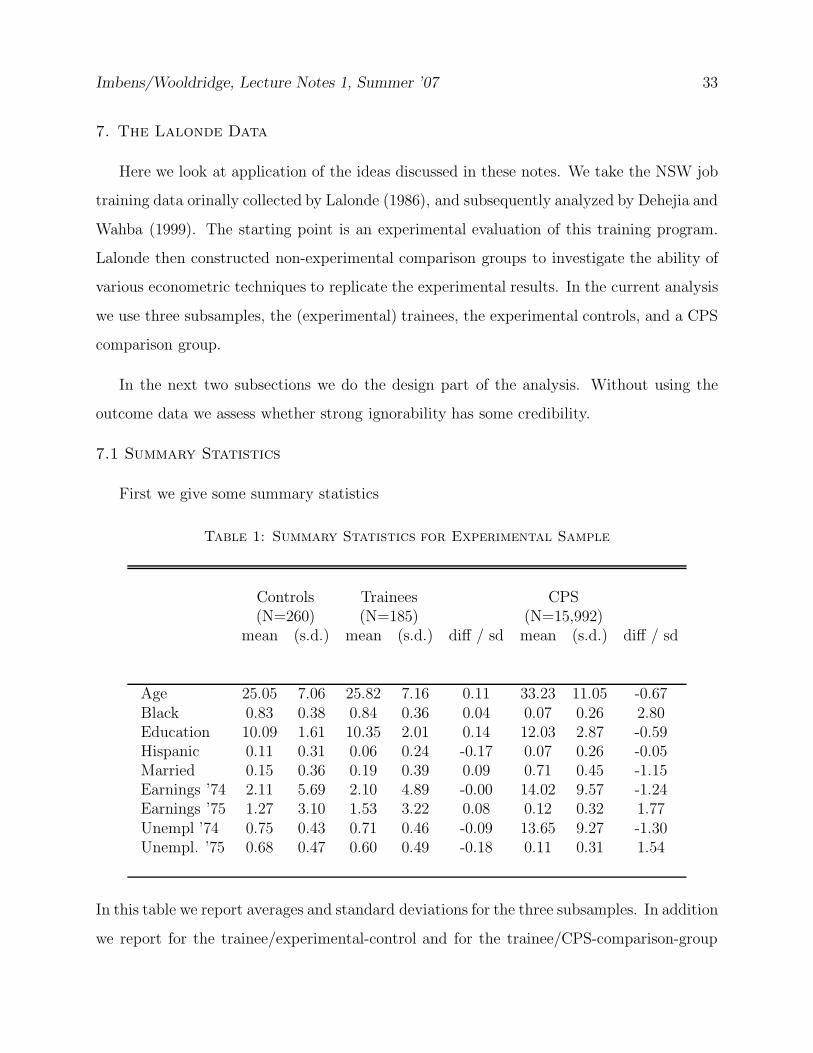
Table 1: Summary Statistics for Experimental Sample
Controls Trainees CPS(N=260) (N=185) (N=15,992)
mean (s.d.) mean (s.d.) diff / sd mean (s.d.) diff / sd
Age 25.05 7.06 25.82 7.16 0.11 33.23 11.05 -0.67Black 0.83 0.38 0.84 0.36 0.04 0.07 0.26 2.80Education 10.09 1.61 10.35 2.01 0.14 12.03 2.87 -0.59Hispanic 0.11 0.31 0.06 0.24 -0.17 0.07 0.26 -0.05Married 0.15 0.36 0.19 0.39 0.09 0.71 0.45 -1.15Earnings ’74 2.11 5.69 2.10 4.89 -0.00 14.02 9.57 -1.24Earnings ’75 1.27 3.10 1.53 3.22 0.08 0.12 0.32 1.77Unempl ’74 0.75 0.43 0.71 0.46 -0.09 13.65 9.27 -1.30Unempl. ’75 0.68 0.47 0.60 0.49 -0.18 0.11 0.31 1.54
In this table we report averages and standard deviations for the three subsamples. In addition
we report for the trainee/experimental-control and for the trainee/CPS-comparison-group
Imbens/Wooldridge, Lecture Notes 1, Summer ’07 34
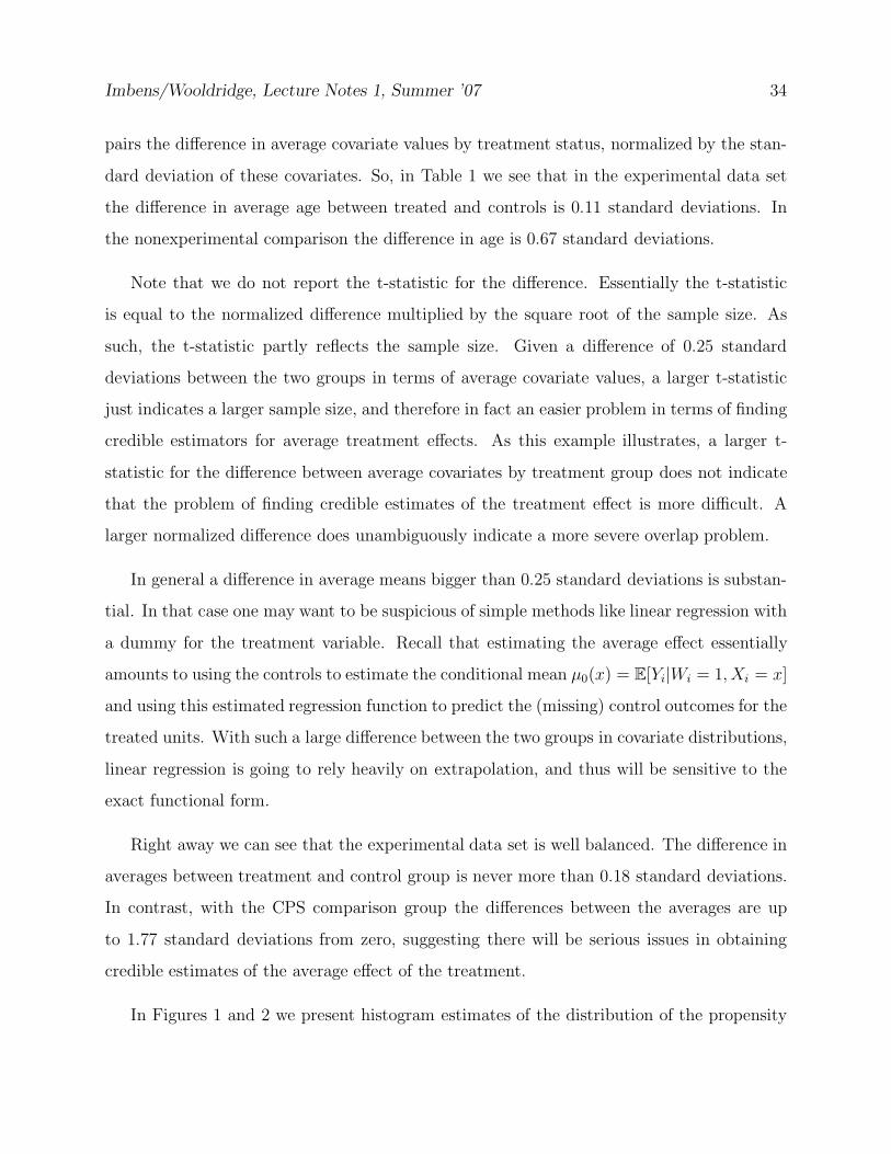
pairs the difference in average covariate values by treatment status, normalized by the stan-
dard deviation of these covariates. So, in Table 1 we see that in the experimental data set
the difference in average age between treated and controls is 0.11 standard deviations. In
the nonexperimental comparison the difference in age is 0.67 standard deviations.
Note that we do not report the t-statistic for the difference. Essentially the t-statistic
is equal to the normalized difference multiplied by the square root of the sample size. As
such, the t-statistic partly reflects the sample size. Given a difference of 0.25 standard
deviations between the two groups in terms of average covariate values, a larger t-statistic
just indicates a larger sample size, and therefore in fact an easier problem in terms of finding
credible estimators for average treatment effects. As this example illustrates, a larger t-
statistic for the difference between average covariates by treatment group does not indicate
that the problem of finding credible estimates of the treatment effect is more difficult. A
larger normalized difference does unambiguously indicate a more severe overlap problem.
In general a difference in average means bigger than 0.25 standard deviations is substan-
tial. In that case one may want to be suspicious of simple methods like linear regression with
a dummy for the treatment variable. Recall that estimating the average effect essentially
amounts to using the controls to estimate the conditional mean µ0(x) = E[Yi|Wi = 1, Xi = x]
and using this estimated regression function to predict the (missing) control outcomes for the
treated units. With such a large difference between the two groups in covariate distributions,
linear regression is going to rely heavily on extrapolation, and thus will be sensitive to the
exact functional form.
Right away we can see that the experimental data set is well balanced. The difference in
averages between treatment and control group is never more than 0.18 standard deviations.
In contrast, with the CPS comparison group the differences between the averages are up
to 1.77 standard deviations from zero, suggesting there will be serious issues in obtaining
credible estimates of the average effect of the treatment.
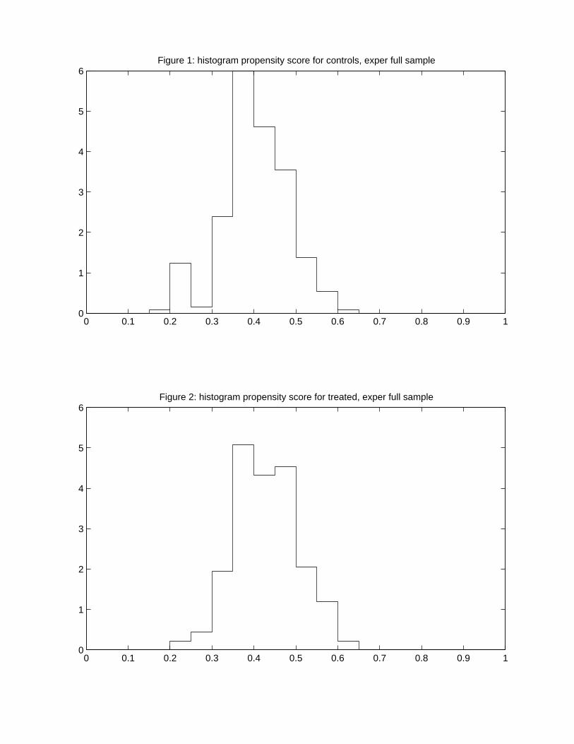
In Figures 1 and 2 we present histogram estimates of the distribution of the propensity
0 0.1 0.2 0.3 0.4 0.5 0.6 0.7 0.8 0.9 10
1
2
3
4
5
6Figure 1: histogram propensity score for controls, exper full sample
0 0.1 0.2 0.3 0.4 0.5 0.6 0.7 0.8 0.9 10
1
2
3
4
5
6Figure 2: histogram propensity score for treated, exper full sample
0 0.2 0.4 0.6 0.8 10
2
4
6
8
10
12
14
16
18
20Figure 3: hist p−score for controls, cps full sample
0 0.2 0.4 0.6 0.8 10
0.5
1
1.5
2
2.5
3
3.5
4Figure 4: hist p−score for treated, cps full sample
0 0.2 0.4 0.6 0.8 10
1
2
3
4
5
6Figure 5: hist p−score for controls, cps selected sample
0 0.2 0.4 0.6 0.8 10
0.5
1
1.5
2
2.5
3
3.5
4
4.5
5Figure 6: hist p−score for treated, cps selected sample
Imbens/Wooldridge, Lecture Notes 1, Summer ’07 35
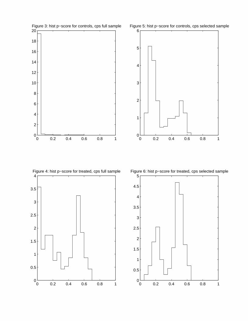
score for the treatment and control group in the experimental Lalonde data. These distri-
butions again suggest that there is considerable overlap in the covariate distributions. In
Figures 3 and 4 we present the histogram estimates for the propensity score distributions for
the CPS comparison group. Now there is a clear lack of overlap. For the CPS comparison
group almost all mass of the propensity score distribution is concentrated in a small interval
to the right of zero, and the distribution for the treatment group is much more spread out.
7.2 Assessing Unconfoundedness
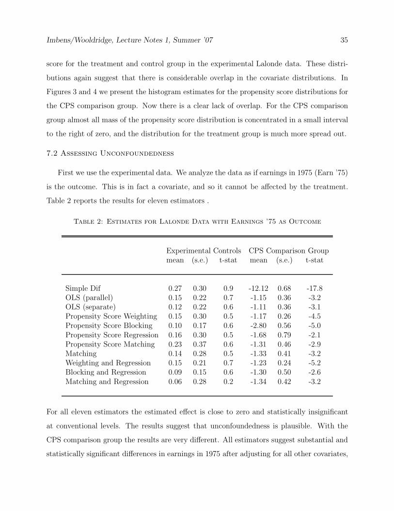
First we use the experimental data. We analyze the data as if earnings in 1975 (Earn ’75)
is the outcome. This is in fact a covariate, and so it cannot be affected by the treatment.
Table 2 reports the results for eleven estimators .
Table 2: Estimates for Lalonde Data with Earnings ’75 as Outcome
Experimental Controls CPS Comparison Groupmean (s.e.) t-stat mean (s.e.) t-stat
Simple Dif 0.27 0.30 0.9 -12.12 0.68 -17.8OLS (parallel) 0.15 0.22 0.7 -1.15 0.36 -3.2OLS (separate) 0.12 0.22 0.6 -1.11 0.36 -3.1Propensity Score Weighting 0.15 0.30 0.5 -1.17 0.26 -4.5Propensity Score Blocking 0.10 0.17 0.6 -2.80 0.56 -5.0Propensity Score Regression 0.16 0.30 0.5 -1.68 0.79 -2.1Propensity Score Matching 0.23 0.37 0.6 -1.31 0.46 -2.9Matching 0.14 0.28 0.5 -1.33 0.41 -3.2Weighting and Regression 0.15 0.21 0.7 -1.23 0.24 -5.2Blocking and Regression 0.09 0.15 0.6 -1.30 0.50 -2.6Matching and Regression 0.06 0.28 0.2 -1.34 0.42 -3.2
For all eleven estimators the estimated effect is close to zero and statistically insignificant
at conventional levels. The results suggest that unconfoundedness is plausible. With the
CPS comparison group the results are very different. All estimators suggest substantial and
statistically significant differences in earnings in 1975 after adjusting for all other covariates,
Imbens/Wooldridge, Lecture Notes 1, Summer ’07 36
including earnings in 1974. This suggests that relying on the unconfoundedness assumption,
in combination with these estimators, is not very credible for this sample.
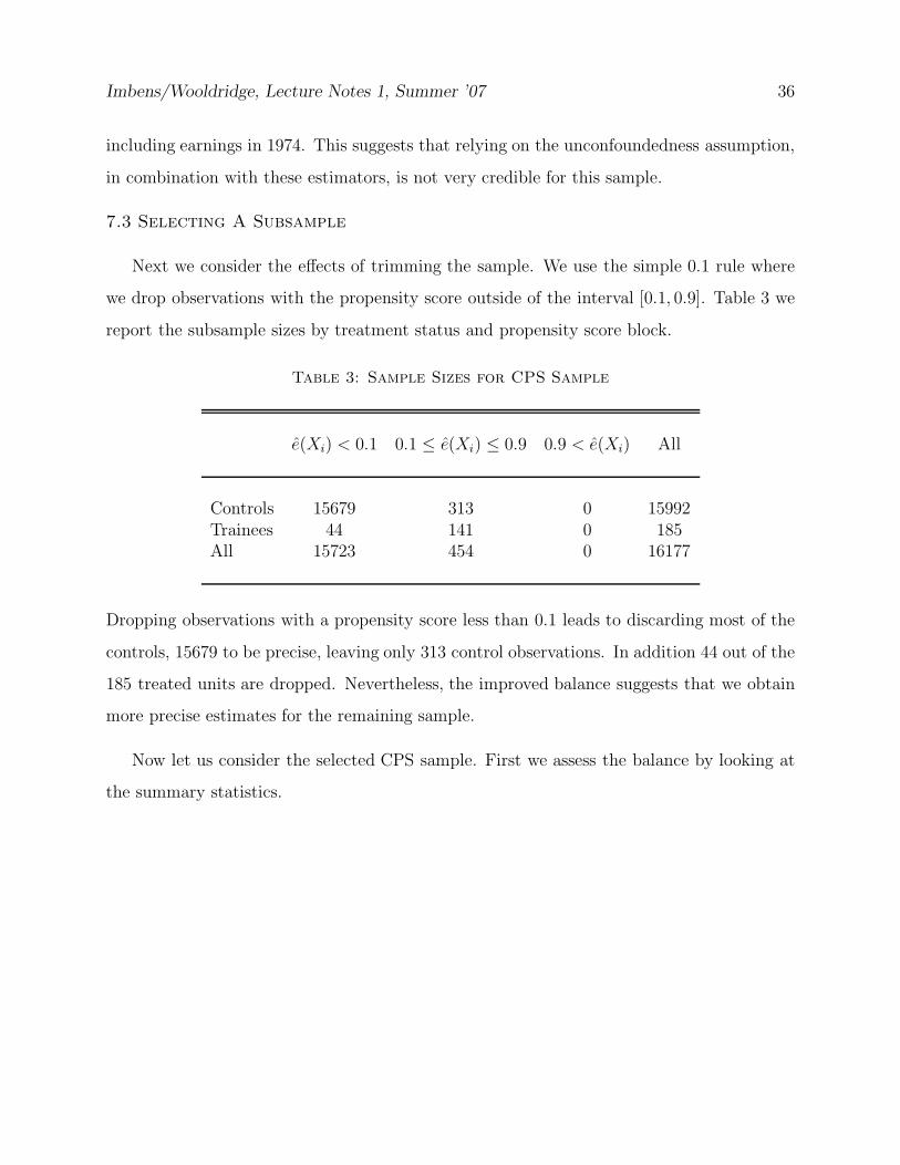
7.3 Selecting A Subsample
Next we consider the effects of trimming the sample. We use the simple 0.1 rule where
we drop observations with the propensity score outside of the interval [0.1, 0.9]. Table 3 we
report the subsample sizes by treatment status and propensity score block.
Table 3: Sample Sizes for CPS Sample
e(Xi) < 0.1 0.1 ≤ e(Xi) ≤ 0.9 0.9 < e(Xi) All
Controls 15679 313 0 15992Trainees 44 141 0 185All 15723 454 0 16177
Dropping observations with a propensity score less than 0.1 leads to discarding most of the
controls, 15679 to be precise, leaving only 313 control observations. In addition 44 out of the
185 treated units are dropped. Nevertheless, the improved balance suggests that we obtain
more precise estimates for the remaining sample.
Now let us consider the selected CPS sample. First we assess the balance by looking at
the summary statistics.
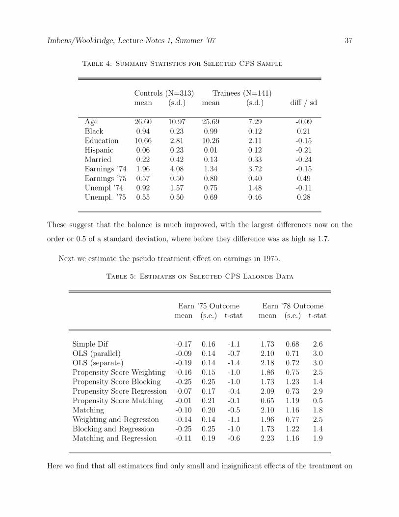
Imbens/Wooldridge, Lecture Notes 1, Summer ’07 37
Table 4: Summary Statistics for Selected CPS Sample
Controls (N=313) Trainees (N=141)mean (s.d.) mean (s.d.) diff / sd
Age 26.60 10.97 25.69 7.29 -0.09Black 0.94 0.23 0.99 0.12 0.21Education 10.66 2.81 10.26 2.11 -0.15Hispanic 0.06 0.23 0.01 0.12 -0.21Married 0.22 0.42 0.13 0.33 -0.24Earnings ’74 1.96 4.08 1.34 3.72 -0.15Earnings ’75 0.57 0.50 0.80 0.40 0.49Unempl ’74 0.92 1.57 0.75 1.48 -0.11Unempl. ’75 0.55 0.50 0.69 0.46 0.28
These suggest that the balance is much improved, with the largest differences now on the
order or 0.5 of a standard deviation, where before they difference was as high as 1.7.
Next we estimate the pseudo treatment effect on earnings in 1975.
Table 5: Estimates on Selected CPS Lalonde Data
Earn ’75 Outcome Earn ’78 Outcomemean (s.e.) t-stat mean (s.e.) t-stat
Simple Dif -0.17 0.16 -1.1 1.73 0.68 2.6OLS (parallel) -0.09 0.14 -0.7 2.10 0.71 3.0OLS (separate) -0.19 0.14 -1.4 2.18 0.72 3.0Propensity Score Weighting -0.16 0.15 -1.0 1.86 0.75 2.5Propensity Score Blocking -0.25 0.25 -1.0 1.73 1.23 1.4Propensity Score Regression -0.07 0.17 -0.4 2.09 0.73 2.9Propensity Score Matching -0.01 0.21 -0.1 0.65 1.19 0.5Matching -0.10 0.20 -0.5 2.10 1.16 1.8Weighting and Regression -0.14 0.14 -1.1 1.96 0.77 2.5Blocking and Regression -0.25 0.25 -1.0 1.73 1.22 1.4Matching and Regression -0.11 0.19 -0.6 2.23 1.16 1.9
Here we find that all estimators find only small and insignificant effects of the treatment on

Imbens/Wooldridge, Lecture Notes 1, Summer ’07 38
earnings in 1975. This suggests that for this sample unconfoundedness may well be a rea-
sonable assumption, and that the estimators considered here can lead to credible estimates.
Finally we report the estimates for earnings in 1978. Only now do we use the outcome data.
Note that with the exclusion of the propensity score matching estimator the estimates are
all between 1.73 and 2.23, and thus relatively insensitive to the choice of estimator.
Imbens/Wooldridge, Lecture Notes 1, Summer ’07 39
References
Athey, S., and S. Stern, (1998), “An Empirical Framework for Testing Theories
About Complementarity in Organizational Design”, NBER working paper 6600.
Blundell, R. and M. Costa-Dias (2002), “Alternative Approaches to Evaluation in
Empirical Microeconomics,”Institute for Fiscal Studies, Cemmap working paper cwp10/02.
Chen, X., H. Hong, and Tarozzi, (2005), “Semiparametric Efficiency in GMM Mod-
els of Nonclassical Measurement Errors, Missing Data and Treatment Effects,”unpublished
working paper, Department of Economics, New York University.
Crump, R., V. J. Hotz, V. J., G. Imbens, and O.Mitnik, (2006), “Moving the
Goalposts: Addressing Limited Overlap in Estimation of Average Treatment Effects by
Changing the Estimand,”unpublished manuscript, Department of Economics, UC Berkeley.
Crump, R., V. J. Hotz, V. J., G. Imbens, and O.Mitnik, (2007), “Nonparametric
Tests for Treatment Effect Heterogeneity,”forthcoming, Review of Economics and Statistics.
Dehejia, R. (2005) “Program Evaluation as a Decision Problem,”Journal of Economet-
rics, 125, 141-173.
Engle, R., D. Hendry, and J.-F. Richard, (1983) “Exogeneity,”Econometrica,
51(2): 277-304.
Firpo, S. (2003), “Efficient Semiparametric Estimation of Quantile Treatment Effects,”
Econometrica, 75(1), 259-276.
Hahn, J., (1998), “On the Role of the Propensity Score in Efficient Semiparametric
Estimation of Average Treatment Effects,” Econometrica 66 (2), 315-331.
Heckman, J., and J. Hotz, (1989), ”Alternative Methods for Evaluating the Impact
of Training Programs”, (with discussion), Journal of the American Statistical Association.,
Vol. 84, No. 804, 862-874.
Heckman, J., and R. Robb, (1985), “Alternative Methods for Evaluating the Impact
Imbens/Wooldridge, Lecture Notes 1, Summer ’07 40
of Interventions,”in Heckman and Singer (eds.), Longitudinal Analysis of Labor Market Data,
Cambridge, Cambridge University Press.
Heckman, J., H. Ichimura, and P. Todd, (1998), “Matching as an Econometric
Evaluation Estimator,” Review of Economic Studies 65, 261–294.
Heckman, J., R. Lalonde, and J. Smith (2000), “The Economics and Econometrics
of Active Labor Markets Programs,”in A. Ashenfelter and D. Card eds. Handbook of Labor
Economics, vol. 3. New York: Elsevier Science.
Hirano, K., and J. Porter, (2005), “Asymptotics for Statistical Decision Rules,”Working
Paper, Dept of Economics, University of Wisconsin.
Hirano, K., G. Imbens, and G. Ridder, (2003), “Efficient Estimation of Average
Treatment Effects Using the Estimated Propensity Score,” Econometrica, 71(4): 1161-1189.
July
Imbens, G. (2000), “The Role of the Propensity Score in Estimating Dose-Response
Functions,”Biometrika, Vol. 87, No. 3, 706-710.
Imbens, G., (2004), “Nonparametric Estimation of Average Treatment Effects Under
Exogeneity: A Review,”Review of Economics and Statistics, 86(1): 1-29.
Imbens, G., and J. Wooldridge., (2007), “Recent Developments in the Economet-
rics of Program Evaluation,”unpublished manuscript, department of economics, Harvard
University.
Lalonde, R.J., (1986), “Evaluating the Econometric Evaluations of Training Programs
with Experimental Data,”American Economic Review, 76, 604-620.
Lechner, M., (2001), “Identification and Estimation of Causal Effects of Multiple
Treatments under the Conditional Independence Assumption,”in Lechner and Pfeiffer (eds.),
Econometric Evaluations of Active Labor Market Policies in Europe, Heidelberg, Physica.
Manski, C., (1990), “Nonparametric Bounds on Treatment Effects,”American Economic
Imbens/Wooldridge, Lecture Notes 1, Summer ’07 41
Review Papers and Proceedings, 80, 319-323.
Manski, C. (2003), Partial Identification of Probability Distributions, New York: Springer-
Verlag.
Manski, C., (2004), “Statistical Treatment Rules for Heterogenous Populations,”Econometrica,
72(4), 1221-1246.
Manski, C. (2005), Social Choice with Partial Knowledge of Treatment Response, Prince-
ton University Press.
Manski, C., G. Sandefur, S. McLanahan, and D. Powers (1992), “Alternative
Estimates of the Effect of Family Structure During Adolescence on High School,”Journal of
the American Statistical Association, 87(417):25-37.
Robins, J., and Y. Ritov, (1997), “Towards a Curse of Dimensionality Appropriate
(CODA) Asymptotic Theory for Semi-parametric Models,”Statistics in Medicine 16, 285-
319.
Rosenbaum, P., (1987), ”The role of a second control group in an observational study”,
Statistical Science, (with discussion), Vol 2., No. 3, 292–316.
Rosenbaum, P., (1995), Observational Studies, Springer Verlag, New York.
Rosenbaum, P., and D. Rubin, (1983a), “The Central Role of the Propensity Score
in Observational Studies for Causal Effects”, emphBiometrika, 70, 41-55.
Rosenbaum, P., and D. Rubin, (1983b), “Assessing the Sensitivity to an Unobserved
Binary Covariate in an Observational Study with Binary Outcome,” Journal of the Royal
Statistical Society, Ser. B, 45, 212-218.
Rubin, D., (1973a), “Matching to Remove Bias in Observational Studies”, Biometrics,
29, 159-183.
Rubin, D., (1973b), “The Use of Matched Sampling and Regression Adjustments to
Remove Bias in Observational Studies”, Biometrics, 29, 185-203.
Imbens/Wooldridge, Lecture Notes 1, Summer ’07 42
Rubin, D. (1974), “Estimating Causal Effects of Treatments in Randomized and Non-
randomized Studies,”Journal of Educational Psychology, 66, 688-701.
Rubin, D., (1977), “Assignment to Treatment Group on the Basis of a Covariate,”Journal
of Educational Statistics, 2(1), 1-26.
Rubin, D. B., (1978), “Bayesian inference for causal effects: The Role of Randomiza-
tion”, Annals of Statistics, 6:34–58.
Rubin, D., (1990), “Formal Modes of Statistical Inference for Causal Effects”, em-
phJournal of Statistical Planning and Inference, 25, 279-292.
Imbens/Wooldridge, Lecture Notes 2, Summer ’07
What’s New in Econometrics? NBER, Summer 2007Lecture 2, Monday, July 30th, 11.00-12.30 am
Linear Panel Data ModelsThese notes cover some recent topics in linear panel data models. They begin with a
“modern” treatment of the basic linear model, and then consider some embellishments, such asrandom slopes and time-varying factor loads. In addition, fully robust tests for correlatedrandom effects, lack of strict exogeneity, and contemporaneous endogeneity are presented.Section 4 considers estimation of models without strictly exogenous regressors, and Section 5presents a unified framework for analyzing pseudo panels (constructed from repeated crosssections).1. Quick Overview of the Basic Model
Most of these notes are concerned with an unobserved effects model defined for a largepopulation. Therefore, we assume random sampling in the cross section dimension. Unlessstated otherwise, the asymptotic results are for a fixed number of time periods, T, with thenumber of cross section observations, N, getting large.
For some of what we do, it is critical to distinguish the underlying population model ofinterest and the sampling scheme that generates data that we can use to estimate the populationparameters. The standard model can be written, for a generic i in the population, as
yit t xit ci uit, t 1, . . . ,T, (1.1)
where t is a separate time period intercept (almost always a good idea), xit is a 1 K vector ofexplanatory variables, ci is the time-constant unobserved effect, and the uit : t 1, . . . ,T areidiosyncratic errors. Thanks to Mundlak (1978) and Chamberlain (1982), we view the ci asrandom draws along with the observed variables. Then, one of the key issues is whether ci iscorrelated with elements of xit.
It probably makes more sense to drop the i subscript in (1.1), which would emphasize thatthe equation holds for an entire population. But (1.1) is useful to emphasizing which factorschange only across t, which change only change across i, and which change across i and t.It issometimes convenient to subsume the time dummies in x it.
Ruling out correlation (for now) between uit and xit, a sensible assumption iscontemporaneous exogeneity conditional on ci :
Euit|xit,ci 0, t 1, . . . ,T. (1.2)
This equation really defines in the sense that under (1.1) and (1.2),
1
Imbens/Wooldridge, Lecture Notes 2, Summer ’07
Eyit|xit,ci t xit ci, (1.3)
so the j are partial effects holding fixed the unobserved heterogeneity (and covariates other
than xtj).
As is now well known, is not identified only under (1.2). Of course, if we addedCovxit,ci 0 for any t, then is identified and can be consistently estimated by a crosssection regression using period t. But usually the whole point is to allow the unobserved effectto be correlated with time-varying xit.
We can allow general correlation if we add the assumption of strict exogeneity conditionalon ci:
Euit|xi1,xi2, . . . ,xiT,ci 0, t 1, . . . ,T, (1.4)
which can be expressed as
Eyit|xi1, . . . ,xiT,ci Eyit|xit,ci t xit ci. (1.5)
If the elements of xit : t 1, . . . ,T have suitable time variation, can be consistentlyestimated by fixed effects (FE) or first differencing (FD), or generalized least squares (GLS) orgeneralized method of moments (GMM) versions of them. If the simpler methods are used, andeven if GLS is used, standard inference can and should be made fully robust toheteroksedasticity and serial dependence that could depend on the regressors (or not). Theseare the now well-known “cluster” standard errors. With large N and small T, there is littleexcuse not to compute them.
(Note: Some call (1.4) or (1.5) “strong” exogeneity. But in the Engle, Hendry, and Richard(1983) work, strong exogeneity incorporates assumptions on parameters in differentconditional distributions being variation free, and that is not needed here.)
The strict exogeneity assumption is always violated if xit contains lagged dependentvariables, but it can be violated in other cases where xi,t1 is correlated with uit – a “feedbackeffect.” An assumption more natural than strict exogeneity is sequential exogeneity conditionon ci:
Euit|xi1,xi2, . . . ,xit,ci 0, t 1, . . . ,T (1.6)
or
Eyit|xi1, . . . ,xit,ci Eyit|xit,ci t xit ci. (1.7)
This allows for lagged dependent variables (in which case it implies that the dynamics in the
2
Imbens/Wooldridge, Lecture Notes 2, Summer ’07
mean have been completely specified) and, generally, is more natural when we take the viewthat xit might react to shocks that affect yit. Generally, is identified under sequentialexogeneity. First differencing and using lags of xit as instruments, or forward filtering, can beused in simple IV procedures or GMM procedures. (More later.)
If we are willing to assume ci and xi are uncorrelated, then many more possibilities arise(including, of course, identifying coefficients on time-constant explanatory variables). Themost convenient way of stating the random effects (RE) assumption is
Eci|xi Eci, (1.8)
although using the linear projection in place of Eci|xi suffices for consistency (but usualinference would not generally be valid). Under (1.8), we can used pooled OLS or any GLSprocedure, including the usual RE estimator. Fully robust inference is available and shouldgenerally be used. (Note: The usual RE variance matrix, which depends only on c
2 and u2,
need not be correctly specified! It still makes sense to use it in estimation but make inferencerobust.)
It is useful to define two correlated random effects assumptions:
Lci|xi xi, (1.9)
which actually is not an assumption but a definition. For nonlinear models, we will have toactually make assumptions about Dci|xi, the conditional distribution. Methods based on (1.9)are often said to implement the Chamberlain device, after Chamberlain (1982).
Mundlak (1978) used a restricted version, and used a conditional expectation:
Eci|xi xi, (1.10)
where xi T−1∑ t1T xit. This formulation conserves on degrees of freedom, and extensions are
useful for nonlinear models.If we write ci xi ai or ci xi ai and plug into the original equation, for
example
yit t xit xi ai uit (1.11)
(absorbing into the time intercepts), then we are tempted to use pooled OLS, or REestimation because Eai uit|xi 0. Either of these leads to the FE estimator of , and to asimple test of H0 : 0. Later, when we discuss control function methods, it will be handy torun regressions directly that include the time averages. (Somewhat surprisingly, obtain the
3
Imbens/Wooldridge, Lecture Notes 2, Summer ’07
same algebraic equivalence using Chamberlain’s devise. The pooled OLS estimator of is stillthe FE estimator, even though the t might change substantially across t.)
Some of us have been pushing for several years the notion that specification tests should bemade robust to assumptions that are not directly being tested. (Technically, they should berobust to assumptions that they have no asymptotic power for detecting violations of.) Muchprogress has been made, but one still sees Hausman statistics computed that maintain a full setof assumptions under the null. Take comparing random effects to fixed effects. The keyassumption is (1.8). whether Varvi|xi has the random effects structure, where vit ci uit,should not be a critical issue. It makes no sense to report a fully robust variance matrix for FEand RE but then to compute a Hausman test that maintains the full set of RE assumptions. (Inaddition to (1.4) and (1.8), these are Varui|xi,ci u
2IT and Varci|xi Varci. ) Theregression-based Hausman test from (1.11) is very handy for obtaining a fully robust test.More specifically, suppose the model contains a full set of year intercepts as well astime-constant and time-varying explanatory variables:
yit gt zi wit ci uit.
Now, it is clear that, because we cannot estimate by FE, it is not part of the Hausman test
comparing RE and FE. What is less clear, but also true, is that the coefficients on the timedummies, , cannot be included, either. (RE and FE estimation only with aggregate time
effects are identical.) In fact, we can only compare the M 1 estimates of , say FE and RE. Ifwe include FE and RE we introduce a nonsingularity in the asymptotic variance matrix. The
regression based test, from the pooled regression
yit on gt, zi, wit, wi, t 1, . . . ,T; i 1, . . . ,N
makes this clear (and that the are M restrictions to test). (Mundlak (1978) suggested this testand Arellano (1993) described the robust version.). Unfortunately, the usual form of theHausman test does not, and, for example, Stata gets it wrong and tries to include the yeardummies in the test (in addition to being nonrobust). The most important problem is thatunwarranted degrees of freedom are added to the chi-square distribution, often many extra df,which can produce seriously misleading p-values.2. New Insights Into Old Estimators
In the past several years, the properties of traditional estimators used for linear models,particularly fixed effects and its instrumental variable counterparts, have been studied under
4
Imbens/Wooldridge, Lecture Notes 2, Summer ’07
weaker assumptions. We review some of those results here. In these notes, we focus on modelswithout lagged dependent variables or other non-strictly exogenous explanatory variables,although the instrumental variables methods applied to linear models can, in some cases, beapplied to models with lagged dependent variables.
2.1. Fixed Effects Estimation in the Correlated Random Slopes Model
The fixed effects (FE) estimator is still the workhorse in empirical studies that employpanel data methods to estimate the effects of time-varying explanatory variables. Theattractiveness of the FE estimator is that it allows arbitrary correlation between the additive,unobserved heterogeneity and the explanatory variables. (Pooled methods that do not removetime averages, as well as the random effects (RE) estimator, essentially assume that theunobserved heterogeneity is uncorrelated with the covariates.) Nevertheless, the framework inwhich the FE estimator is typically analyzed is somewhat restrictive: the heterogeneity isassumed to be additive and is assumed to have a constant coefficients (factor loads) over time.Recently, Wooldridge (2005a) has shown that the FE estimator, and extensions that sweepaway unit-specific trends, has robustness properties for estimating the population averageeffect (PAE) or average partial effect (APE).
We begin with an extension of the usual model to allow for unit-specific slopes,
yit ci xitbi uit
Euit|xi,ci,bi 0, t 1, . . . ,T, (2.1) (2.2)
where bi is K 1. Rather than acknowledge that bi is unit-specific, we ignore theheterogeneity in the slopes and act as if bi is constant for all i. We think ci might be correlatedwith at least some elements of xit, and therefore we apply the usual fixed effects estimator. Thequestion we address here is: when does the usual FE estimator consistently estimate thepopulation average effect, Ebi.
In addition to assumption (2.2), we naturally need the usual FE rank condition,
rank ∑t1
T
Exit′ xit K. (2.3)
Write bi di where the unit-specific deviation from the average, di, necessarily has a zeromean. Then
yit ci xit xitdi uit ≡ ci xit vit (2.4)
where vit ≡ xitdi uit. A sufficient condition for consistency of the FE estimator along with
5
Imbens/Wooldridge, Lecture Notes 2, Summer ’07
(3) is
Exit′ vit 0, t 1, . . . ,T. (2.5)
Along with (2.2), it suffices that Exit′ xitdi 0 for all t. A sufficient condition, and one that is
easier to interpret, is
Ebi|xit Ebi , t 1, . . . ,T. (2.6)
Importantly, condition (2.6) allows the slopes, bi, to be correlated with the regressors xit
through permanent components. What it rules out is correlation between idiosyncraticmovements in xit. We can formalize this statement by writing xit fi r it, t 1, . . . ,T. Then
(2.6) holds if Ebi|r i1,r i2, . . . ,r iT Ebi. So bi is allowed to be arbitrarily correlated with thepermanent component, fi. (Of course, xit fi r it is a special representation of the covariates,
but it helps to illustrate condition (2.6).) Condition (2.6) is similar in spirit to the Mundlak(1978) assumption applied to the slopes (rather to the intercept):Ebi|xi1,xi2, . . . ,xiT Ebi|xi
One implication of these results is that it is a good idea to use a fully robust variance matrixestimator with FE even if one thinks idiosyncratic errors are serially uncorrelated: the termxitdi is left in the error term and causes heteroskedasticity and serial correlation, in general.
These results extend to a more general class of estimators that includes the usual fixedeffects and random trend estimator. Write
yit wtai xitbi uit, t 1, . . . ,T (2.7)
where wt is a set of deterministic functions of time. We maintain the standard assumption (2.2)but with ai in place of ci. Now, the “fixed effects” estimator sweeps away ai by netting out wt
from xit. In particular, now let xit denote the residuals from the regression xit onwt, t 1, . . . ,T.
In the random trend model, wt 1, t, and so the elements of xit have unit-specific lineartrends removed in addition to a level effect. Removing even more of the heterogeneity fromxit makes it even more likely that (2.6) holds. For example, if xit fi hit r it, then bi can
be arbitrarily correlated with fi,hi. Of course, individually detrending the xit requires at least
three time periods, and it decreases the variation in xit compared to the usual FE estimator. Notsurprisingly, increasing the dimension of wt (subject to the restriction dimwt T), generallyleads to less precision of the estimator. See Wooldridge (2005a) for further discussion.
Of course, the first differencing transformation can be used in place of, or in conjunction
6
Imbens/Wooldridge, Lecture Notes 2, Summer ’07
with, unit-specific detrending. For example, if we first difference followed by the withintransformation, it is easily seen that a condition sufficient for consistency of the resultingestimator for is
Ebi|Δxit Ebi, t 2, . . . ,T, (2.8)
where Δxit Δxit − Δx are the demeaned first differences.Now consider an important special case of the previous setup, where the regressors that
have unit-specific coefficients are time dummies. We can write the model as
yit xit tci uit, t 1, . . . ,T, (2.9)
where, with small T and large N, it makes sense to treat t : t 1, . . . ,T as parameters, like. Model (2.9) is attractive because it allows, say, the return to unbobserved “talent” to changeover time. Those who estimate, say, firm-level production functions like to allow theimportance of unobserved factors, such as managerial skill, to change over time. Estimation of, along with the t, is a nonlinear problem. What if we just estimate by fixed effects? Letc Eci and write (2.9) as
yit t xit tdi uit, t 1, . . . ,T, (2.10)
where t tc and di ci − c has zero mean In addition, the composite error,vit ≡ tdi uit, is uncorrelated with xi1,x2, . . . ,xiT (as well as having a zero mean). It is easyto see that consistency of the usual FE estimator, which allows for different time periodintercepts, is ensured if
Covxit,ci 0, t 1, . . . ,T. (2.11)
In other words, the unobserved effects is uncorrelated with the deviations xit xit − xi.If we use the extended FE estimators for random trend models, as above, then we can
replace xit with detrended covariates. Then, ci can be correlated with underlying levels andtrends in xit (provided we have a sufficient number of time periods).
Using usual FE (with full time period dummies) does not allow us to estimate the t, oreven determine whether the t change over time. Even if we are interested only in when ci
and xit are allowed to be correlated, being able to detect time-varying factor loads is importantbecause (2.11) is not completely general. It is useful to have a simple test ofH0 : 2 3 . . . T with some power against the alternative of time-varying coefficients.Then, we can determine whether a more sophisticated estimation method might be needed.
We can obtain a simple variable addition test that can be computed using linear estimation
7
Imbens/Wooldridge, Lecture Notes 2, Summer ’07
methods if we specify a particular relationship between ci and xi. We use the Mundlak (1978)assumption
ci xi ai. (2.12)
Then
yit t xit txi tai uit t xit xi txi ai tai uit, (2.13)
where t t − 1 for all t. Under the null hypothesis, t 0, t 2, . . . ,T. If we impose thenull hypothesis, the resulting model is linear, and we can estimate it by pooled OLS of yit on1,d2t, . . . ,dTt,xit, xi across t and i, where the drt are time dummies. A variable addition testthat all t are zero can be obtained by applying FE to the equation
yit 1 2d2t . . .TdTt xit 2d2txi . . .TdTtxi errorit, (2.14)
and test the joint significance of the T − 1 terms d2txi, . . . ,dTtxi. (The term xi would
drop out of an FE estimation, and so we just omit it.) Note that xi is a scalar and so the test asT − 1 degrees of freedom. As always, it is prudent to use a fully robust test (even though, underthe null, tai disappears from the error term).
A few comments about this test are in order. First, although we used the Mundlak device toobtain the test, it does not have to represent the actual linear projection because we are simplyadding terms to an FE estimation. Under the null, we do not need to restrict the relationshpbetween ci and xi. Of course, the power of the test may be affected by this choice. Second, thetest only makes sense if ≠ 0; in particular, it cannot be used in a pure random effectsenvironment. Third, a rejection of the null does not necessarily mean that the usual FEestimator is inconsistent for : assumption (11) could still hold. In fact, the change in theestimate of when the interaction terms are added can be indicative of whether accounting for
time-varying t is likely to be important. But, because has been estimated under the null, theestimated from (1.14) is not generally consistent.
If we want to estimate the t along with , we can impose the Mundlak assumption andestimate all parameteres, including , by pooled nonlinear regression or some GMM version.Or, we can use Chamberlain’s (1982) less restrictive assumption. But, typically, when we wantto allow arbitrary correlation between ci and xi, we work directly from (9) and eliminate the ci.There are several ways to do this. If we maintain that all t are different from zero then we canuse a quas-differencing method to eliminat ci. In particular, for t ≥ 2 we can multiply the t − 1equation by t/ t−1 and subtract the result from the time t equation:
8
Imbens/Wooldridge, Lecture Notes 2, Summer ’07
yit − t/ t−1yi,t−1 xit− t/ t−1xi,t−1 tci − t/ t−1 t−1ci uit − t/ t−1ui,t−1
xit− t/ t−1xi,t−1 uit − t/ t−1ui,t−1, t ≥ 2.
We define t t/ t−1 and write
yit − tyi,t−1 xit − txi,t−1 eit, t 2, . . . ,T, (2.15)
where eit ≡ uit − tui,t−1. Under the strict exogeneity assumption, eit is uncorrelated with everyelement of xi, and so we can apply GMM to (2.15) to estimate and 2, . . . ,T. Again, thisrequires using nonlinear GMM methods, and the eit would typically be serially correlated. Ifwe do not impose restrictions on the second moment matrix of ui, then we would not use anyinformation on the second moments of ei; we would (eventually) use an unrestricted weightingmatrix after an initial estimation.
Using all of xi in each time period can result in too many overidentifying restrictions. Attime t we might use, say, zit xit,xi,t−1, and then the instrument matrix Zi (with T − 1 rows)would be diagzi2, . . . ,ziT. An initial consistent estimator can be gotten by choosing weighting
matrix N−1∑ i1N Zi
′Zi−1. Then the optimal weighting matrix can be estimated. Ahn, Lee, and
Schmidt (2002) provide further discussion.If xit contains sequentially but not strictly exogenous explanatory variables – such as a
lagged dependent variable – the instruments at time t can only be chosen from xi,t−1, . . . ,xi1.Holtz-Eakin, Newey, and Rosen (1988) explicitly consider models with lagged dependentvariables; more on these models later.
Other transformations can be used. For example, at time t ≥ 2 we can use the equation
t−1yit − tyi,t−1 t−1xit − txi,t−1 eit, t 2, . . . ,T,
where now eit t−1uit − tui,t−1. This equation has the advantage of allowing t 0 for somet. The same choices of instruments are available depending on whether xit are strictly orsequentially exogenous.
2.2. Fixed Effects IV Estimation with Random Slopes
The results for the fixed effects estimator (in the generalized sense of removingunit-specific means and possibly trends), extend to fixed effects IV methods, provided we adda constant conditional covariance assumption. Murtazashvili and Wooldridge (2007) derive asimple set of sufficient conditions. In the model with general trends, we assume the naturalextension of Assumption FEIV.1, that is, Euit|zi,ai,bi 0 for all t, along with AssumptionFEIV.2. We modify assumption (2.6) in the obvious way: replace xit with zit, the
9
Imbens/Wooldridge, Lecture Notes 2, Summer ’07
invididual-specific detrended instruments:
Ebi|zit Ebi , t 1, . . . ,T (2.16)
But something more is needed. Murtazashvili and Wooldridge (2007) show that, along with theprevious assumptions, a sufficient condition is
Covxit,bi|zit Covxit,bi, t 1, . . . ,T. (2.17)
Note that the covariance Covxit,bi, a K K matrix, need not be zero, or even constant acrosstime. In other words, we can allow the detrended covariates to be arbitrarily correlated with theheterogeneous slopes, and that correlation can change in any way across time. But theconditional covariance cannot depend on the time-demeaned instruments. (This is an exampleof how it is important to distinguish between a conditional expectation and an unconditionalone: the implicit error in the equation generally has an unconditional mean that changes with t,but its conditional mean does not depend on zit, and so using zit as IVs is valid provided weallow for a full set of dummies.) Condition (2.17) extends to the panel data case theassumption used by Wooldridge (2003a) in the cross section case.
We can easily show why (2.17) suffices with the previous assumptions. First, ifEdi|zit 0 – which follows from Ebi|zit Ebi – then Covxit,di|zit Exitdi
′|zit, andso Exitdi|zit Exitdi ≡ t under the previous assumptions. Write xitdi t rit whereEriti|zit 0, t 1, . . . ,T. Then we can write the transformed equation as
ÿit xit xitdi üit ÿit xit t rit üit. (2.18)
Now, if xit contains a full set of time period dummies, then we can absorb t into xit, and weassume that here. Then the sufficient condition for consistency of IV estimators applied to thetransformed equations is Ezit
′ rit üit 0,.and this condition is met under the maintainedassumptions. In other words, under (2.16) and (2.17), the fixed effects 2SLS estimator isconsistent for the average population effect, . (Remember, we use “fixed effects” here in thegeneral sense of eliminating the unit-specific trends, ai.) We must remember to include a fullset of time period dummies if we want to apply this robustness result, something that should bedone in any case. Naturally, we can also use GMM to obtain a more efficient estimator. If bi
truly depends on i, then the composite error rit üit is likely serially correlated andheteroskedastic. See Murtazashvili and Wooldridge (2007) for further discussion andsimilation results on the peformance of the FE2SLS estimator. They also provide exampleswhere the key assumptions cannot be expected to hold, such as when endogenous elements of
10
Imbens/Wooldridge, Lecture Notes 2, Summer ’07
xit are discrete.3. Behavior of Estimators without Strict Exogeneity
As is well known, both the FE and FD estimators are inconsistent (with fixed T, N → )without the conditional strict exogeneity assumption. But it is also pretty well known that, atleast under certain assumptions, the FE estimator can be expected to have less “bias” (actually,inconsistency) for larger T. One assumption is contemporaneous exogeneity, (1.2). If wemaintain this assumption, assume that the data series xit,uit : t 1, . . . ,T is “weaklydependent” – in time series parlance, integrated of order zero, or I(0) – then we can show that
plim FE OT−1
plim FD O1.
(3.1)
(3.2)
In some special cases – the AR(1) model without extra covariates – the “bias” terms can becalculated. But not generally. The FE (within) estimator averages across T, and this tends toreduce the bias.
Interestingly, the same results can be shown if xit : t 1, . . . ,T has unit roots as long asuit is I(0) and contemporaneous exogeneity holds. But there is a catch: if uit is I(1) – sothat the time series version of the “model” would be a spurious regression (yit and xit are notcointegrated), then (3.1) is no longer true. And, of course, the first differencing means any unitroots are eliminated. So, once we start appealing to “large T” to prefer FE over FD, we muststart being aware of the time series properties of the series.
The same comments hold for IV versions of the estimators. Provided the instruments arecontemporaneously exogenous, the FEIV estimator has bias of order T−1, while the bias in theFDIV estimator does not shrink with T. The same caveats about applications to unit rootprocesses also apply.
Because failure of strict exogeneity causes inconsistency in both FE and FD estimation, itis useful to have simple tests. One possibility is to obtain a Hausman test directly comparingthe FE and FD estimators. This is a bit cumbersome because, when aggregate time effects areincluded, the difference in the estimators has a singular asymptotic variance. Plus, it issomewhat difficult to make the test fully robust.
Instead, simple regression-based strategies are available. Let wit be the 1 Q vector, asubset of xit suspected of failing strict exogeneity. A simple test of strict exogeneity,specifically looking for feedback problems, is based on
11
Imbens/Wooldridge, Lecture Notes 2, Summer ’07
yit t xit wi,t1 ci eit, t 1, . . . ,T − 1. (3.3)
Estimate the equation by fixed effects and test H0 : 0 (using a fully robust test). Of course,the test may have little power for detecting contemporaneous endogeneity.
In the context of FEIV we can test whether a subset of instruments fails strict exogeneityby writing
yit t xit hi,t1 ci eit, t 1, . . . ,T − 1, (3.4)
where hit is a subset of the instruments, zit. Now, estimate the equation by FEIV usinginstruments zit,hi,t1 and test coefficients on the latter.
It is also easy to test for contemporaneous endogeneity of certain regressors, even if weallow some regressors to be endogenous under the null. Write the model now as
yit1 zit11 yit21 yit31 ci1 uit1, (3.5)
where, in an FE environment, we want to test H0 : Eyit3′ uit1 0 . Actually, because we are
using the within transformation, we are really testing strict exogeneity of yit3, but we allow all
variables to be correlated with ci1. The variables yit2 are allowed to be endogenous under the
null – provided, of course, that we have sufficient instruments excluded from the structuralequation that are uncorrelated with uit1 in every time period. We can write a set of reducedforms for elements of yit3 as
yit3 zit3 c i3 vit3, (3.6)
and obtain the FE residuals,v it3 ÿit3 − zit3, where the columns of 3 are the FE estimates
of the reduced forms, and the double dots denotes time-demeaning, as usual. Then, estimatethe equation
ÿit1 zit11 ÿit21 ÿit31 v it31 errorit1 (3.7)
by pooled IV, using instruments zit,ÿit3,v it3. The test of the null that yit3 is exogenous is just
the (robust) test that 1 0, and the usual robust test is valid with adjusting for the first-step
estimation.
An equivalent approach is to define vit3 yit3 − zit3, where 3 is still the matrix of FE
coefficients, add these to equation (3.5), and apply FE-IV, using a fully robust test. Using abuilt-in command can lead to problems because the test is rarely made robust and the degreesof freedom are often incorrectly counted.4. Instrumental Variables Estimation under Sequential Exogeneity
12
Imbens/Wooldridge, Lecture Notes 2, Summer ’07
We now consider IV estimation of the model
yit xit ci uit, t 1, . . . ,T, (4.1)
under sequential exogeneity assumptions. Some authors simply use
Exis′ uit 0, s 1, . . . ,T, t 1, . . . ,T. (4.2)
As always, xit probably includes a full set of time period dummies. This leads to simplemoment conditions after first differencing:
Exis′ Δuit 0, s 1, . . . , t − 1; t 2, . . . ,T. (4.3)
Therefore, at time t, the available instruments in the FD equation are in the vector xi,t−1o , where
xito ≡ xi1,xi2, . . . ,xit. (4.4)
Therefore, the matrix of instruments is simply
Wi diagxi1o ,xi2
o , . . . ,xi,T−1o , (4.5)
which has T − 1 rows. Because of sequential exogeneity, the number of valid instrumentsincreases with t.
Given Wi, it is routine to apply GMM estimation. But some simpler strategies are availablethat can be used for comparison or as the first-stage estimator in computing the optimalweighting matrix. One useful one is to estimate a reduced form for Δxit separately for each t.
So, at time t, run the regression Δxit on xi,t−1o , i 1, . . . ,N, and obtain the fitted values, Δxit. Of
course, the fitted values are all 1 K vectors for each t, even though the number of availableinstruments grows with t. Then, estimate the FD equation
Δyit Δxit Δuit, t 2, . . . ,T (4.6)
by pooled IV using instruments (not regressors) Δxit. It is simple to obtain robust standarderrors and test statistics from such a procedure because the first stage estimation to obtain theinstruments can be ignored (asymptotically, of course).
One potential problem with estimating the FD equation by IVs that are simply lags of xit isthat changes in variables over time are often difficult to predict. In other words, Δxit mighthave little correlation with xi,t−1
o , in which case we face a problem of weak instruments. In one
case, we even lose identification: if xit t xi,t−1 e it where Ee it|xi,t−1, . . . ,xi1 0 – that is,the elements of xit are random walks with drift – then EΔxit|xi,t−1, . . . ,xi1 0, and the rankcondition for IV estimation fails.
13
Imbens/Wooldridge, Lecture Notes 2, Summer ’07
If we impose what is generally a stronger assumption, dynamic completeness in theconditional mean,
Euit|xit,yi,t−1xi,t−1, . . . ,yi1,xi1,ci 0, t 1, . . . ,T, (4.7)
then more moment conditions are available. While (4.7) implies that virtually any nonlinearfunction of the xit can be used as instruments, the focus has been only on zero covarianceassumptions (or (4.7) is stated as a linear projection). The key is that (4.7) implies thatuit : t 1, . . . ,T is a serially uncorrelated sequence and uit is uncorrelated with ci for all t. Ifwe use these facts, we obtain moment conditions first proposed by Ahn and Schmidt (1995) inthe context of the AR(1) unosberved effects model; see also Arellano and Honoré (2001). Theycan be written generally as
EΔyi,t−1 − Δxi,t−1 ′yit − xit 0, t 3, . . . ,T. (4.8)
Why do these hold? Because all uit are uncorrelated with ci, and ui,t−1, . . . ,ui1 areuncorrelated with ci uit. So ui,t−1 − ui,t−2 is uncorrelated with ci uit, and the resultingmoment conditions can be written in terms of the parameters as (4.8). Therefore, under (4.7),we can add the conditions (4.8) to (4.3) to improve efficiency – in some cases quitesubstantially with persistent data.
Of course, we do not always intend for models to be dynamically complete in the sense of(4.7). Often, we estimate static models or finite distributed lag models – that is, models withoutlagged dependent variables – that have serially correlated idiosyncratic errors, and theexplanatory variables are not strictly exogenous and so GLS procedures are inconsistent. Plus,the conditions in (4.8) are nonlinear in parameters.
Arellano and Bover (1995) suggested instead the restrictions
CovΔxit′ ,ci 0, t 2, . . . ,T. (4.9)
Interestingly, this is zero correlation, FD version of the conditions from Section 2 that implywe can ignore heterogeneous coefficients in estimation under strict exogeneity. Under (4.9),we have the moment conditions from the levels equation:
EΔxit′ yit − − xit 0, t 2, . . . ,T, (4.10)
because yit − xit ci uit and uit is uncorrelated with xit and xi,t−1. We add an intercept, ,explicitly to the equation to allow a nonzero mean for ci. Blundell and Bond (1999) applythese moment conditions, along with the usual conditions in (4.3), to estimate firm-levelproduction functions. Because of persistence in the data, they find the moments in (4.3) are not
14
Imbens/Wooldridge, Lecture Notes 2, Summer ’07
especially informative for estimating the parameters. Of course, (4.9) is an extra set ofassumptions.
The previous discussion can be applied to the AR(1) model, which has received muchattention. In its simplest form we have
yit yi,t−1 ci uit, t 1, . . . ,T, (4.11)
so that, by convention, our first observation on y is at t 0. Typically the minimal assumptionsimposed are
Eyisuit 0, s 0, . . . , t − 1, t 1, . . . ,T, (4.12)
in which case the available instruments at time t are wit yi0, . . . ,yi,t−2 in the FD equation
Δyit Δyi,t−1 Δuit, t 2, . . . ,T. (4.13)
In oher words, we can use
EyisΔyit − Δyi,t−1 0, s 0, . . . , t − 2, t 2, . . . ,T. (4.14)
Anderson and Hsiao (1982) proposed pooled IV estimation of the FD equation with the singleinstrument yi,t−2 (in which case all T − 1 periods can be used) or Δyi,t−2 (in which case onlyT − 2 periods can be used). We can use pooled IV where T − 1 separate reduced forms are
estimated for Δyi,t−1 as a linear function of yi0, . . . ,yi,t−2. The fitted values Δyi,t−1, can be used
as the instruments in (4.13) in a pooled IV estimation. Of course, standard errors and inferenceshould be made robust to the MA(1) serial correlation in Δuit. Arellano and Bond (1991)suggested full GMM estimation using all of the available instruments yi0, . . . ,yi,t−2, and thisestimator uses the conditions in (4.12) efficiently.
Under the dynamic completeness assumption
Euit|yi,t−1,yi,t−2, . . . ,yi0,ci 0, (4.15)
the Ahn-Schmidt extra moment conditions in (4.8) become
EΔyi,t−1 − Δyi,t−2yit − yi,t−1 0, t 3, . . . ,T. (4.16)
Blundell and Bond (1998) noted that if the condition
CovΔyi1,ci Covyi1 − yi0,ci 0 (4.17)
is added to (4.15) then the combinded set of moment conditions becomes
EΔyi,t−1yit − − yi,t−1 0, t 2, . . . ,T, (4.18)
which can be added to the usual moment conditions (4.14). Therefore, we have two sets of
15
Imbens/Wooldridge, Lecture Notes 2, Summer ’07
moments linear in the parameters. The first, (4.14), use the differenced equation while thesecond, (4.18), use the levels. Arellano and Bover (1995) analyzed GMM estimators fromthese equations generally.
As discussed by Blundell and Bond (1998), condition (4.17) can be intepreted as arestriction on the initial condition, yi0. To see why, writeyi1 − yi0 yi0 ci ui1 − yi0 1 − yi0 ci ui1. Because ui1 is uncorrelated with ci,(4.17) becomes
Cov1 − yi0 ci,ci 0. (4.19)
Write yi0 as a deviation from its steady state, ci/1 − (obtained for || 1 be recursivesubsitution and then taking the limit), as
yi0 ci/1 − ri0. (4.20)
Then 1 − yi0 ci 1 − ri0, and so (4.17) reduces to
Covri0,ci 0. (4.21)
In other words, the deviation of yi0 from its steady state is uncorrelated with the steady state.Blundell and Bond (1998) contains discussion of when this condition is reasonable. Of course,it is not for 1, and it may not be for “close” to one. On the other hand, as shown byBlundell and Bond (1998), this restriction, along with the Ahn-Schmidt conditions, is veryinformative for close to one. Hahn (1999) shows theoretically that such restrictions cangreatly increase the information about .
The Ahn-Schmidt conditions (4.16) are attractive in that they are implied by the mostnatural statement of the model, but they are nonlinear and therefore more difficult to use. Byadding the restriction on the initial condition, the extra moment condition also means that thefull set of moment conditions is linear. Plus, this approach extends to general models with onlysequentially exogenous variabes as in (4.10). Extra moment assumptions based onhomoskedasticity assumptions – either conditional or unconditional – have not been usednearly as much, probably because they impose conditions that have little if anything to do withthe economic hypotheses being tested.
Other approaches to dynamic models are based on maximum likelihood estimation orgeneralized least squares estimation of a particular set of conditional means. Approaches thatcondition on the initial condition yi0, an approach suggested by Chamberlain (1980), Blundelland Smith (1991), and Blundell and Bond (1998), seem especially attractive. For example,
16
Imbens/Wooldridge, Lecture Notes 2, Summer ’07
suppose we assume that
Dyit|yi,t−1,yi,t−2, . . . ,yi1,yi0,ci Normalyi,t−1 ci,u2, t 1,2, . . . ,T.
Then the distribution of yi1, . . . ,yiT given yi0 y0,ci c is just the product of the normaldistributions:
t1
T
u−Tyt − yt−1 − c/u.
We can obtain a usable density for (conditional) MLE by assuming
ci|yi0 ~Normal0 0yi0,a2.
The log likelihood function is obtained by taking the log of
−
t1
T
1/uTyit − yi,t−1 − c/u. 1/ac − 0 − 0yi0/adc.
Of course, if this is this represents the correct density of yi1, . . . ,yiT given yi0 then the MLE isconsistent and N -asymptotically normal (and efficient among estimators that condition onyi0.
A more robust approach is to use a generalized least squares approach where Eyi|yi0 and
Varyi|yi0 are obtained, and where the latter could even be misspecified. Like with the MLE
approach, this results in estimation that is highly nonlinear in the parameters and is used lessoften than the GMM procedures with linear moment conditions.
The same kinds of moment conditions can be used in extensions of the AR(1) model, suchas
yit yi,t−1 zit ci uit, t 1, . . . ,T.
If we difference to remove ci, we can then use exogeneity assumptions to choose instruments.The FD equation is
Δyit Δyi,t−1 Δzit Δuit, t 1, . . . ,T,
and if the zit are strictly exogenous with respect to ui1, . . . ,uiT then the available instruments(in addition to time period dummies) are zi,yi,t−2, . . . ,yi0. We might not want to use all of zi
for every time period. Certainly we would use Δzit, and perhaps a lag, Δzi,t−1. If we addsequentially exogenous variables, say hit, to (11.62) then hi,t−1, . . . ,hi1 would be added to thelist of instruments (and Δhit would appear in the equation). We might also add the Arellano
17

Imbens/Wooldridge, Lecture Notes 2, Summer ’07
and Bover conditions (4.10), or at least the Ahn and Schmidt conditions (4.8).As a simple example of methods for dynamic models, consider a dynamic air fare equation
for routes in the United States:
lfareit t lfarei,t−1 concenit ci uit,
where we include a full set of year dummies. We assume the concentration ratio, concenit, isstrictly exogenous and that at most one lag of lfare is needed to capture the dynamics. The dataare for 1997 through 2000, so the equation is specified for three years. After differencing, wehave only two years of data:
Δlfareit t Δlfarei,t−1 Δconcenit Δuit, t 1999,2000.
If we estimate this equation by pooled OLS, the estimators are inconsistent because Δlfarei,t−1
is correlated with Δuit; we include the OLS estimates for comparison. We apply the simplepooled IV procedure, where separate reduced forms are estimated for Δlfarei,t−1: one for 1999,with lfarei,t−2 and Δconcenit in the reduced form, and one for 2000, with lfarei,t−2, lfareimt−3 andΔconcenit in the reduced form. The fitted values are used in the pooled IV estimation, withrobust standard errors. (We only use Δconcenit in the IV list at time t.) Finally, we apply theArellano and Bond (1991) GMM procedure.
Dependent Variable: lfare
(1) (2) (3)
Explanatory Variable Pooled OLS Pooled IV Arellano-Bond
lfare−1 −. 126 . 219 . 333
. 027 . 062 . 055
concen . 076 . 126 . 152
. 053 . 056 . 040
N 1, 149 1, 149 1, 149
As is seen from column (1), the pooled OLS estimate of is actually negative andstatistically different from zero. By contrast, the two IV methods give positive and statisticallysignificant estimates. The GMM estimate of is larger, and it also has a smaller standard error(as we would hope for GMM).
The previous example has small T, but some panel data applications have reasonable largeT. Arellano and Alvarez (1998) show that the GMM estimator that accounts for the MA(1)serial correlation in the FD errors has desirable properties when T and N are both large, while
18
Imbens/Wooldridge, Lecture Notes 2, Summer ’07
the pooled IV estimator is actually inconsistent under asymptotics where T/N → a 0. SeeArellano (2003, Chapter 6) for discussion.5. Pseudo Panels from Pooled Cross Sections
In cases where panel data sets are not available, we can still estimate parameters in anunderlying panel population model if we can obtain random samples in different periods.Many surveys are done annually by obtaining a different random (or stratified) sample for eachyear. Deaton (1985) showed how to identify and estimate parameters in panel data modelsfrom pooled cross sections. As we will see, however, identification of the parameterse can betenuous.
Deaton (1985) was careful about distinguishing between the population model on the onehand and the sampling scheme on the other. This distinction is critical for understanding thenature of the identification problem, and in deciding the appropriate asymptotic analysis. Therecent literature has tended to write “models” at the cohort or group level, which is not in thespirit of Deaton’s original work. (Angrist (1991) actually has panel data, but uses averages ineach t to estimate parameters of a labor supply function.)
In what follows, we are interested in estimating the parameters of the population model
yt t xt f ut, t 1, . . . ,T, (5.1)
which is best viewed as representing a population defined over T time periods. For this setup tomake sense, it must be the case that we can think of a stationary population, so that the sameunits are represented in each time period. Because we allow a full set of period intercepts, Efis never separately identified, and so we might as well set it to zero.
The random quantities in (5.1) are the response variable, yt, the covariates, xt (a 1 Kvector), the unobserved effect, f, and the unobserved idiosyncratic errors, ut : t 1, . . . ,T.Like our previous analysis, we are thinking of applications with a small number of timeperiods, and so we view the intercepts, t, as parameters to estimate, along with the K 1vector parameter – which is ultimately of interest. We consider the case where all elements ofxt have some time variation.
As it turns out, to use the standard analysis, we do not even have to assumecontemporaneous exogeneity conditional on f, that is,
Eut|xt, f 0, t 1, . . . ,T, (5.2)
although this is a good starting point to determine reasonable population assumptions.
19
Imbens/Wooldridge, Lecture Notes 2, Summer ’07
Naturally, iterated expectations implies
Eut|f 0, t 1, . . . ,T, (5.3)
and (5.3) is sensible in the context of (5.1). Unless stated otherwise, we take it to be true.Because f aggregates all time-constant unobservables, we should think of (5.3) as implying thatEut|g 0 for any time-constant variable g, whether unobserved or observed. In other words,in the leading case we should think of (5.1) as representing Eyt|xt, f where any time constantfactors are lumped into f.
With a (balanced) panel data set, we would have a random sample in the cross section.Therefore, for a random draw i , x it,yit, t 1, . . . ,T, we would then write the model as
yit t xit fi uit, t 1, . . . ,T. (5.4)
While this notation can cause confusion later when we sample from each cross section, it hasthe benefit of explictly labelling quantities as changing only across t, changing only across i, orchanging across both.
The idea of using independent cross sections to estimate parameters from panel datamodels is based on a simple insight of Deaton’s. Assume that the population for which (5.1)holds is divided into G groups (or cohorts). This designation cannot depend on time. Forexample, it is common to birth year to define the groups, or even ranges of birth year. For arandom draw i satisfying (5.4), let gi be the group indicator, taking on a value in 1,2, . . . ,G.Then, by our earlier discussion,
Euit|gi 0, t 1, . . . ,T, (5.5)
essentially by definition. In other words, the t account for any change in the averageunobservables over time and fi accounts for any time-constant factors.
Taking the expected value of (5.4) conditional on group membership and using only (5.5),we have
Eyit|gi g t Exit|gi g Efi|gi g, t 1, . . . ,T. (5.6)
Again, this expession represents an underlying population, but where we have partitioned thepopulation into G groups.
Several authors after Deaton, including Collado (1997) and Verbeek and Vella (2005),have left Euit|gi g as part of the “error term,” with the notation ugt
∗ Euit|gi g. In fact,
these authors have criticized previous work by Moffitt (1993) for making the “asssumption”that ugt
∗ 0. But, as Deaton showed, if we start with the underlying population model (5.1),
20
Imbens/Wooldridge, Lecture Notes 2, Summer ’07
then Euit|gi g 0 for all g follows directly. Nevertheless, as we will discuss later, the keyassumption is that the structural model (5.1) does not require a full set of group/time effects. Ifsuch effects are required, then one way to think about the resulting misspecification is thatEuit|gi g is not zero.
If we define the population means
g Efi|gi ggt
y Eyit|gi ggt
x Exit|gi g (5.7)
for g 1, . . . ,G and t 1, . . . ,T we have
gty t gt
x g, g 1, . . . ,G, t 1, . . . ,T. (5.8)
(Many authors use the notation ygt∗ in place of gt
y , and similarly for gtx , but, at this point, such
a notation gives the wrong impression that the means defined in (5.7) are random variables.They are not. They are group/time means defined on the underlying population.)
Equation (5.8) is remarkable in that it holds without any assumptions restricting thedependence between xit and uir across t and r. In fact, xit can contain lagged dependentvariables, most commonly yi,t−1, or explanatory variables that are contemporaneouslyendogenous (as occurs under measurement error in the original population model, an issue thatwas important to Angrist (1991)). This probably should make us a little suspicious, as theproblems of lagged dependent variable, measurement error, and other violations of strictexogeneity are tricky to handle with true panel data.
(In estimation, we will deal with the fact that there are not really T G parameters in t
and g to estimate; there are only T G − 1. The lost degree of freedom comes from Ef 0,
which puts a restriction on the g. With the groups of the same size in the population, the
restriction is that the g sum to zero.)
If we take (5.8) as the starting point for estimating (along with t and g, then the issues
become fairly clear. If we have sufficient observations in the group/time cells, then the meansgt
y and gtx can be estimated fairly precisly, and these can be used in a minimum distance
estimation framework to estimate , where consists of , , and (where, say, we set 1 0as the normalization).
Before discussing estimation details, it is useful to study (5.8) in more detail to determinesome simple, and common, strategies. Because (5.8) looks itself like a panel data regression
21
Imbens/Wooldridge, Lecture Notes 2, Summer ’07
equation, methods such as “OLS,” “fixed effects,” and “first differencing” have been appliedto sample averages. It is informative to apply these to the population. First suppose that we seteach g to zero and set all of the time intercepts, t, to zero. For notational simplicity, we also
drop an overall “intercept,” but that would be included at a minimum. Then gty gt
x and if
we premultiply by gtx′, average across g and t, and then assume we can invert
∑g1G ∑ t1
T gtx′gt
x , we have
∑g1
G
∑t1
T
gtx′gt
x
−1
∑g1
G
∑t1
T
gtx′gt
y . (5.9)
This means that the population parameter, , can be written as a pooled OLS regression of thepopulation group/time means gt
y on the group/time means gtx . Naturally, if we have “good”
estimates of these means, then it will make sense to estimate by using the same regression onthe sample means. But, so far, this is all in the population. We can think of (5.9) as the basisfor a method of moments procedure. It is important that we treat gt
x and gty symetrically, that
is, as population means to be estimated, whether the xit are strictly, sequentially, orcontemporaneous exogenous – or none of these – in the original model.
When we allow different group means for fi, as seems critical, and different time periodintercepts, which also is necessary for a convincing analysis, we can easily write as an“OLS” estimator by subtracting of time and group averages. While we cannot claim that theseexpressions will result in efficient estimators, they can shed light on whether we can expect(5.8) to lead to precise estimation of . First, without separate time intercepts we have
gty − g
y gtx − g
x, g 1, . . . ,G, ; t 1, . . . ,T, (5.10)
where the notation should be clear, and then one expression for is (5.9) but with gtx − g
x in
place of gtx . Of course, this makes it clear that identification of more difficult when the g
are allowed to differ. Further, if we add in the year intercepts, we have
∑g1
G
∑t1
T
gtx′gt
x
−1
∑g1
G
∑t1
T
gtx′gt
y (5.11)
where gtx is the vector of residuals from the pooled regression
gtx on 1, d2, . . . ,dT, c2, ..., cG, (5.12)
22
Imbens/Wooldridge, Lecture Notes 2, Summer ’07
where dt denotes a dummy for period t and cg is a dummy variable for group g.There are other expressions for , too. (Because is generally overidentified, there are
many ways to write it in terms of the population moments. For example, if we difference andthen take away group averages, we have
∑g1
G
∑t2
T
Δgtx′Δgt
x
−1
∑g1
G
∑t2
T
Δgtx′Δgt
y (5.13)
where Δgtx gt
x − g,t−1x and Δgt
x Δgtx − G−1∑h1
G Δhtx .
Equations (5.11) and (5.13) make it clear that the underlying model in the populationcannot contain a full set of group/time interactions. So, for example, if the groups (cohorts) aredefined by birth year, there cannot be a full set of birth year/time period interactions. We couldallow this feature with invidual-level data because we would typically have variation in thecovariates within each group/period cell. Thus, the absense of full cohort/time effects in thepopulation model is the key an identifying restriction.
Even if we exclude full group/time effects, may not be precisely estimable. Clearly isnot identified if we can write gt
x t g for vectors t and g, t 1, . . . ,T, g 1, . . . ,G. In
other words, while we must exclude a full set of group/time effects in the structural model, weneed some interaction between them in the distribution of the covariates. One might be worriedabout this way of identifying . But even if we accept this identification strategy, the variationin gt
x : t 1, . . ,T, g 1, . . . ,G or Δgtx : t 2, . . ,T, g 1, . . . ,G might not be sufficient
to learn much about – even if we have pretty good estimates of the population means.We are now ready to formally discuss estimation of . We have two formulas (and there
are many more) that can be used directly, once we estimate the group/time means for yt and xt.We can use either true panel data or repeated cross sections. Angrist (1991) used panel dataand grouped the data by time period (after differencing). Our focus here is on the case wherewe do not have panel data, but the general discussion applies to either case. One difference isthat, with independent cross sections, we need not account for dependence in the sampleaverages across g and t (except in the case of dynamic models).
Assume we have a random sample on xt,yt of size Nt, and we have specified the Ggroups or cohorts. Write xit,yit : i 1, . . . ,Nt. Some authors, wanting to avoid confusionwith a true panel data set, prefer to replace i with it to emphasize that the cross section unitsare different in each time period. (Plus, several authors actually write the underlying model in
23
Imbens/Wooldridge, Lecture Notes 2, Summer ’07
terms of the pooled cross sections rather than using the underlying population model – amistake, in my view.) As long as we understand that we have a random sample in each timeperiod, and that random sample is used to estimate the group/time means, there should be noconfusion.
For each random draw i, it is useful to let r i rit1, rit2, . . . , ritG be a vector of groupindicators, so ritg 1 if observation i is in group g. Then the sample average on the response
variable in group/time cell g, t can be written as
gty Ngt
−1∑i1
Nt
ritgyit Ngt/Nt−1Nt−1∑
i1
Nt
ritgyit, (5.14)
where Ngt ∑ i1Nt ritg is properly treated as a random outcome. (This differs from standard
stratified sampling, where the groups are first chosen and then random samples are obtainedwithin each group (stratum). Here, we fix the groups and then randomly sample from thepopulation, keeping track of the group for each draw.) Of course, gt
y is generally consistent for
gty . First, gt Ngt/Nt converges in probability to g Pritg 1 – the fraction of the
population in group or cohort g (which is supposed to be constant across t). So
gt−1Nt
−1∑i1
Nt
ritgyitp→ g
−1Eritgyit
g−1Pritg 1 0 Pritg 1Eyit|ritg 1
Eyit|ritg 1 gty .
Naturally, the argument for other means is the same. Let wit denote the K 1 1 vectoryit,xit ′. Then the asymptotic distribution of the full set of means is easy to obtain:
Nt gtw − gt
w → Normal0,g−1gt
w,
where gtw is the sample average for group/time cell g, t and
gtw Varwt|g
is the K 1 K 1 variance matrix for group/time cell g, t. When we stack the meansacross groups and time periods, it is helpful to have the result
N gtw − gt
w → Normal0, gt−1gtw, (5.15)
where N ∑ t1T Nt and t
N→lim Nt/N is, essentially, the fraction of all observations
accounted for by cross section t. Of course, gt is consistently estimated by Ngt/N, and so, the
24
Imbens/Wooldridge, Lecture Notes 2, Summer ’07
implication of (5.15) is that the sample average for cell g, t gets weighted by Ngt/N, the
fraction of all observations accounted for by cell g, t.In implementing minimum distance estimation, we need a consistent estimator of gt
w , and
the group/time sample variance serves that purpose:
gtw Ngt
−1∑i1
ritgwit − gtwwit − gt
w ′p→ gt
w . (5.16)
Now let be the vector of all cell means. For each g, t, there are K 1 means, and so isa GTK 1 1 vector. It makes sense to stack starting with the K 1 means for g 1,t 1, g 1, t 2, ..., g 1, t T, ..., g G, t 1, ..., g G, t T. Now, the gt
w are always
independent across g because we assume random sampling for each t. When xt does notcontain lags or leads, the gt
w are independent across t, too. (When we allow for lags of the
response variable or explanatory variables, we will adjust the definition of and the momentconditions. Thus, we will always assume that the gt
w are independent across g and t.) Then,
N − →Normal0,, (5.17)
where is the GTK 1 GTK 1 block diagonal matrix with g, t block gtw /gt.
Note that incorporates both different cell variance matrices as well as the differentfrequencies of observations.
The set of equations in (5.8) constitute the restrictions on , , and . Let be theK T G − 1 vector of these parameters, written as
′, ′, ′ ′.
There are GTK 1 restrictions in equations (5.8), so, in general, there are manyoveridentifying restrictions. We can write the set of equations in (5.8) as
h, 0, (5.18)
where h, is a GTK 1 1 vector. Because we have N -asymptotically normal estimator, a minimum distance approach suggests itself. It is different from the usual MD problembecause the parameters do not appear in a separable way, but MD estimation is still possible.In fact, for the current application, h, is linear in each argument, which means MDestimators of are in closed form.
Before obtaining the efficient MD estimator, we need, because of the nonseparability, aninitial consistent estimator of . Probably the most straightforward is the “fixed effects”
25
Imbens/Wooldridge, Lecture Notes 2, Summer ’07
estimator described above, but where we estimate all components of . The estimator uses thejust identified set of equations.
For notational simplicity, let gt denote the K 1 1 vector of group/time means for
each g, t cell. Then let gt be the K T G − 1 1 vector gtx ,dt,cg ′, where dt is a
1 T − 1 vector of time dummies and cg is a 1 G vector of group dummies. Then the
moment conditions are
∑g1
G
∑t1
T
gtgt′ − ∑
g1
G
∑t1
T
gtgty 0. (5.19)
When we plug in – that is, the sample averages for all g, t, then is obtained as theso-called “fixed effects” estimator with time and group effects. The equations can be written as
q, 0, (5.20)
and this representation can be used to find the asymptotic variance of N − ; naturally, itdepends on and is straightforward to estimate.
But there is a practically important point: there is nothing nonstandard about the MDproblem, and bootstrapping is justified for obtaining asymptotic standard errors and teststatistics. (Inoue (forthcoming) asserts that the “unconditional” limiting distribution of
N − is not standard, but that is because he treats the sample means of the covariates andof the response variable differently; in effect, he conditions on the former.) The boostrappingis simple: resample each cross section separately, find the new groups for the bootstrap sample,and obtain the “fixed effects” estimates. It makes no sense here to resampling the groups.
Because of the nonlinear way that the covariate means appear in the estimation, thebootstrap may be preferred. The usual asymptotic normal approximation obtained from
first-order asymptotics may not be especially good in this case, especially if∑g1G ∑ t1
T gtx′gt
x
is close to being singular, in which case is poorly identified. (Inoue (2007) provides evidencethat the distribution of the “FE” estimator, and what he calls a GMM estimator that accountsfor different cell sample sizes, do not appear to be normal even with fairly large cell sizes. Buthis setup for generating the data is different – in particular, he specifies equations directly forthe repeated cross sections, and that is how he generates data. As mentioned above, hisasymptotic analysis differ from the MD framework, and implies nonnormal limitingdistributions. If the data are drawn for each cross section to satisfy the population panel datamodel, the cell sizes are reasonably large, and there is sufficient variation in gt
x , the minimum
26
Imbens/Wooldridge, Lecture Notes 2, Summer ’07
distance estimators should have reasonable finite-sample properties. But because the limiting
distribution depends on thegt
x, which appear in a highly nonlinear way, asymptotic normal
approximation might still be poor.)With the restrictions written as in (5.18), Chamberlain (lecture notes) shows that the
optimal weighting matrix is the inverse of
∇h,∇h, ′, (5.21)
where ∇h, is the GT GTK 1 Jacobian of h, with respect to . (In the standardcase, ∇h, is the identity matrix.) We already have the consistent estimator of – the cellaverages – we showed how to consistently estimate in equations (5.16), and we can use asthe initial consistent estimator of .∇h, ∇h IGT ⊗ −1, ′. Therefore, ∇h,∇h, is a block diagonal
matrix with blocks
−1, ′gt−1gtw −1, ′ ′. (5.22)
But
gt2 ≡ −1, ′gt
w −1, ′ ′ Varyt − xt|g, (5.23)
and a consistent estimator is simply
Ngt−1∑
i1
Nt
ritgyit − xit − t − g2
is the residual variance estimated within cell g, t.Now, ∇h, W, the GT K T G − 1 matrix of “regressors” in the FE
estimation, that is, the rows of W are gt gtx′,dt,cg. Now, the FOC for the optimal MD
estimator is
Ŵ′Ĉ−1Ŵ − gt
y 0,
and so
Ŵ ′Ĉ−1Ŵ−1Ŵ′Ĉ−1
gty . (5.24)
So, as in the standard cases, the efficient MD estimator looks like a “weighted least squares”estimator. The estimated asymptotic variance of , following Chamberlain, is just
Ŵ ′Ĉ−1Ŵ−1/N. Because Ĉ−1 is the diagonal matrix with entries Ngt/N/gt
2 , it is easy to
weight each cell g, t and then compute both and its asymptotic standard errors via a
27
Imbens/Wooldridge, Lecture Notes 2, Summer ’07
weighted regression; fully efficient inference is straightforward. But one must compute the gt2
using the individual-level data in each group/time cell.It is easily seen that the so-called “fixed effects” estimator, , is
Ŵ′Ŵ−1Ŵ′
gty , (5.25)
that is, it uses the identity matrix as the weighting matrix. From Chamberlain (lecture notes),
the asymptotic variance of is estimated as Ŵ′Ŵ−1Ŵ′ČŴŴ′Ŵ
−1, where Č is the matrix
described above but with used to estimate the cell variances. (Note: This matrix cannot becomputed by just using the “heteroskedasticity-robust” standard errors in the regress gt
y on gtx ,
dt, cg.) Because inference using requires calculating the group/time specific variances, we
might as well use the efficient MD estimator in (5.24).Of course, after the efficient MD estimation, we can readily compute the overidentifying
restrictions, which would be rejected if the underlying model needs to include cohort/timeeffects in a richer fashion.
A few remaining comments are in order. First, several papers, including Deaton (1985),Verbeek and Nijman (1993), and Collado (1997), use a different asymptotic analysis. In thecurrent notation, GT → (Deaton) or G → , with the cell sizes fixed. These approachesseems unnatural for the way pseudo panels are constructed, and the thought experiment abouthow one might sample more and more groups is convoluted. While T → conceptually makessense, it is still the case that the available number of time periods is much smaller than thecross section sample sizes for each T. McKenzie (2004) has shown that estimators derivedunder large G asymptotics can have good properties under the MD asymptotics used here. Oneway to see this is that the IV estimators proposed by Collado (1997), Verbeek and Vella(2005), and others are just different ways of using the population moment conditions in (5.8).
(Some authors appear to want it both ways. For example, Verbeek and Nijman (1993) uselarge G asymptotics, but treat the within-cell variances and covariances as known. This stanceassumes that one can get precise estimates of the second moments within each cell, whichmeans that Ngt should be large.)
Basing estimation on (5.8) and using minimum ditance, assuming large cell sizes, makesapplication to models with lags relatively straightforward. The only difference now is that thevectors of means, gt
w : g 1, . . . ,G; t 1, . . . ,T now contain redundancies. (In other
approaches to the problem, for example Collado (1997), McKenzie (2004), the problem with
28
Imbens/Wooldridge, Lecture Notes 2, Summer ’07
adding yt−1 to the population model is that it generates correlation in the estimating equationbased on the pooled cross sections. Here, there is no conceptual distinction between havingexogenous or endogenous elements in xt; all that matters is how adding one modifies the MDmoment conditions. As an example, suppose we write
yt t yt−1 zt f ut
Eut|g 0, g 1, . . . ,G (5.26)
where g is the group number. Then (5.8) is still valid. But, now we would define the vector ofmeans as gt
y ,gtz , and appropriately pick off gt
y in defining the moment conditions. The
alternative is to define gtx to include g,t−1
y , but this results in a singularity in the asymptotic
distribution of . It is much more straightforward to keep only nonredundant elements in andreadjust how the moment conditions.are defined in terms of . When we take that approach, itbecomes clear that we now have fewer moments to estimate the parameters. If zt is 1 J, wehave now have J T G parameters to estimate from GTJ 1 population moments. Still, wehave added just one more parameter.
To the best of my knowledge, the treatment here is the first to follow the MD approach,applied to (5.8), to its logical conclusion. Its strength is that the estimation method is widelyknown and used, and it separates the underlyng population model from sampling assumptions.It also shows why we need not make any exogeneity assumptions on xt. Perhaps mostimportantly, it reveals the key identification condition: that separate group/time effects are notneeded in the underlying model, but enough group/time variation in the means Ext|g isneeded to identify the structural parameters. This sort of condition falls out of other approachesto the problem, such as the instrumental variables approach of but it is harder to see. Forexample, Verbeek and Vella (2005) propose instrumental variables methods on the equation intime averages using interactions between group (cohort) and time dummies. With a full set ofseparate time and group effects in the main equation – derivable here from the populationpanel model – the key identification assumption is that a full set of group/time effects can beexcluded from the structural equation, but the means of the covariates have to vary sufficientlyacross group/time. That is exactly the conclusion we reach with a minimum distance approach.
Interestingly, the MD approach applies easily to extensions of the basic model. Forexample, we can allow for unit-specific time trends (as in the random growth model ofHeckman and Hotz (1989)):
29
Imbens/Wooldridge, Lecture Notes 2, Summer ’07
yt t xt f1 f2t ut, (5.27)
where, for a random draw i, the unobserved heterogeneity is of the form fi1 fi2t. Then, usingthe same arguments as before,
gty t gt
x g gt, (5.28)
and this set of moment conditions is easily handled by extending the previous analysis. We caneven estimate models with time-varying factor loads on the heterogeneity:
yt t xt tf ut,
where 1 1 (say) as a normalization. Now the population moments satisfy
gty t gt
x tg.
There are now K G 2T − 1 free parameters to estimate from GTK 1 moments. Thisextension means that the estimating equations allow the group/time effects to enter moreflexibly (although, of course, we cannot replace t tg with unrestricted group/time
effects.) The MD estimation problem is now nonlinear because of the interaction term, tg.
With more parameters and perhaps not much variation in the gtx , practical implementation may
be a problem, but the theory is standard.This literature would benefit from a careful simulation study, where data for each cross
section are generated from the underlying population model, and where gi – the groupidentifier – is randomly drawn, too. To be realistic, the underlying model should have full timeeffects. Verbeek and Vella (2005) come close, but they omit aggregate time effects in the mainmodel while generating the explanatory variables to have means that differ by group/time cell.Probably this paints too optimistic a picture for how well the estimators can work in practice.Remember, even if we can get precise estimates of the cell means, the variation in gt
x across g
and t might not be enough to tie down precisely.Finally, we can come back to the comment about how the moment conditions in (5.8) only
use the assumption Eut|g 0 for all t and g. It seems likely that we should be able to exploitcontemporaneous exogeneity assumptions. Let zt be a set of observed variables such thatEut|zt, f 0, t 1, . . . ,T. (In a true panel, these vary across i and t. We might have zt xt,but perhaps zt is just a subset of xt, or we have extra instruments.) Then we can add to (5.8) themoment conditions
30

Imbens/Wooldridge, Lecture Notes 2, Summer ’07
Ezt′yt|g tEzt|g Ezt
′xt|g Ezt′f|g Ezt
′ut|g tEzt|g Ezt
′xt|g Ezt′f|g, (5.29)
where Ezt′ut|g 0 when we view group designation as contained in f. The moments
Ezt′yt|g, Ezt|g, and Ezt
′xt|g can all be estimated by random samples from each crosssection, where we average within group/time period. (This would not work if xt or zt containslags.) This would appear to add many more moment restrictions that should be useful foridentifying , but that depends on what we assume about the unobserved moments Ezt
′f|g.
References(To be added.)
31
Imbens/Wooldridge, Lecture Notes 3, NBER, Summer ’07 1
What’s New in Econometrics NBER, Summer 2007
Lecture 3, Monday, July 30th, 2.00-3.00pm
Regression Discontintuity Designs1
1. Introduction
Since the late 1990s there has been a large number of studies in economics applying and
extending Regression Discontinuity (RD) methods from its origins in the statistics literature
in the early 60’s (Thisthlewaite and Cook, 1960). Here, we review some of the practical
issues in implementation of RD methods. The focus is on five specific issues. The first
is the importance of graphical analyses as powerful methods for illustrating the design.
Second, we suggest using local linear regression methods using only the observations close
to the discontinuity point. Third, we discuss choosing the bandwidth using cross validation
specifically tailored to the focus on estimation of regression functions on the boundary of the
support, following Ludwig and Miller (2005). Fourth, we provide two simple estimators for
the asymptotic variance, one of them exploiting the link with instrumental variables methods
derived by Hahn, Todd, and VanderKlaauw (2001, HTV). Finally, we discuss a number of
specification tests and sensivitity analyses based on tests for (a) discontinuities in the average
values for covariates, (b) discontinuities in the conditional density of the forcing variable, as
suggested by McCrary (2007), (c) discontinuities in the average outcome at other values of
the forcing variable.
2. Sharp and Fuzzy Regression Discontinuity Designs
2.1 Basics
Our discussion will frame the RD design in the context of the modern literature on causal
effects and treatment effects, using the potential outcomes framework (Rubin, 1974), rather
than the regression framework that was originally used in this literature. For unit i there
are two potential outcomes, Yi(0) and Yi(1), with the causal effect defined as the difference
1These notes draw heavily on Imbens and Lemieux (2007).
Imbens/Wooldridge, Lecture Notes 3, NBER, Summer ’07 2
Yi(1) − Yi(0), and the observed outcome equal to
Yi = (1 − Wi) · Yi(0) + Wi · Yi(1) =
Yi(0) if Wi = 0,Yi(1) if Wi = 1,
where Wi ∈ 0, 1 is the binary indicator for the treatment.
The basic idea behind the RD design is that assignment to the treatment is determined,
either completely or partly, by the value of a predictor (the forcing variable Xi) being on
either side of a common threshold. This predictor Xi may itself be associated with the
potential outcomes, but this association is assumed to be smooth, and so any discontinuity
in the conditional distribution of the outcome, indexed by the value of this covariate at
the cutoff value, is interpreted as evidence of a causal effect of the treatment. The design
often arises from administrative decisions, where the incentives for units to participate in a
program are partly limited for reasons of resource constraints, and clear transparent rules
rather than discretion by administrators are used for the allocation of these incentives.
2.2 The Sharp Regression Discontinuity Design
It is useful to distinguish between two designs, the Sharp and the Fuzzy Regression
Discontinuity (SRD and FRD from hereon) designs (e.g., Trochim, 1984, 2001; HTV). In
the SRD design the assignment Wi is a deterministic function of one of the covariates, the
forcing (or treatment-determining) variable X:
Wi = 1Xi ≥ c.
All units with a covariate value of at least c are in the treatment group (and participation
is mandatory for these individuals), and all units with a covariate value less than c are in
the control group (members of this group are not eligible for the treatment). In the SRD
design we look at the discontinuity in the conditional expectation of the outcome given the
covariate to uncover an average causal effect of the treatment:
limx↓c
E[Yi|Xi = x] − limx↑c
E[Yi|Xi = x] = limx↓c
E[Yi(1)|Xi = x] − limx↑c
E[Yi(0)|Xi = x], (1)
is interpreted as the average causal effect of the treatment at the discontinuity point.
τSRD = E[Yi(1) − Yi(0)|Xi = c]. (2)
Imbens/Wooldridge, Lecture Notes 3, NBER, Summer ’07 3
In order to justify this interpretation we make a smoothness assumption. Typically this
assumption is formulated in terms of conditional expectations2:
Assumption 1 (Continuity of Conditional Regression Functions)
E[Y (0)|X = x] and E[Y (1)|X = x],
are continuous in x.
Under this assumption,
τSRD = limx↓c
E[Yi|Xi = x] − limx↑c
E[Yi|Xi = x].
The estimand is the difference of two regression functions at a point.
There is a unavoidable need for extrapolation, because by design there are no units with
Xi = c for whom we observe Yi(0). We therefore will exploit the fact that we observe units
with covariate values arbitrarily close to c.3
As an example of a SRD design, consider the study of the effect of party affiliation
of a congressman on congressional voting outcomes by Lee (2007). See also Lee, Moretti
and Butler (2004). The key idea is that electoral districts where the share of the vote for a
Democrat in a particular election was just under 50% are on average similar in many relevant
respects to districts where the share of the Democratic vote was just over 50%, but the small
difference in votes leads to an immediate and big difference in the party affiliation of the
elected representative. In this case, the party affiliation always jumps at 50%, making this
is a SRD design. Lee looks at the incumbency effect. He is interested in the probability
2More generally, one might want to assume that the conditional distribution function is smooth in thecovariate. Let FY (w)|X(y|x) = Pr(Yi(w) ≤ y|Xi = x) denote the conditional distribution function of Yi(w)given Xi. Then the general version of the assumption assume that FY (0)|X(y|x) and FY (1)|X(y|x) arecontinuous in x for all y. Both assumptions are stronger than required, as we will only use continuity atx = c, but it is rare that it is reasonable to assume continuity for one value of the covariate, but not at othervalues of the covariate.
3Although in principle the first component in the difference in (1) would be straightforward to estimate ifwe actually observe individuals with Xi = x, with continuous covariates we also need to estimate this termby averaging over units with covariate values close to c.
Imbens/Wooldridge, Lecture Notes 3, NBER, Summer ’07 4
of Democrats winning the subsequent election, comparing districts where the Democrats
won the previous election with just over 50% of the popular vote with districts where the
Democrats lost the previous election with just under 50% of the vote.
2.3 The Fuzzy Regression Discontinuity Design
In the Fuzzy Regression Discontinuity (FRD) design the probability of receiving the
treatment need not change from zero to one at the threshold. Instead the design allows for
a smaller jump in the probability of assignment to the treatment at the threshold:
limx↓c
Pr(Wi = 1|Xi = x) 6= limx↑c
Pr(Wi = 1|Xi = x),
without requiring the jump to equal 1. Such a situation can arise if incentives to participate
in a program change discontinuously at a threshold, without these incentives being powerful
enough to move all units from nonparticipation to participation. In this design we interpret
the ratio of the jump in the regression of the outcome on the covariate to the jump in the
regression of the treatment indicator on the covariate as an average causal effect of the
treatment. Formally, the estimand is
τFRD =limx↓c E[Yi|Xi = x] − limx↑c E[Yi|Xi = x]
limx↓c E[Wi|Xi = x] − limx↑c E[Wi|Xi = x].
As an example of a FRD design, consider the study of the effect of financial aid on
college attendance by VanderKlaauw (2002). VanderKlaauw looks at the effect of financial
aid on acceptance on college admissions. Here Xi is a numerical score assigned to college
applicants based on the objective part of the application information (SAT scores, grades)
used to streamline the process of assigning financial aid offers. During the initial stages of
the admission process, the applicants are divided into L groups based on discretized values
of these scores. Let
Gi =
1 if 0 ≤ Xi < c1
2 if c1 ≤ Xi < c2
...L if cL−1 ≤ Xi
denote the financial aid group. For simplicity, let us focus on the case with L = 2, and a
single cutoff point c. Having a score just over c will put an applicant in a higher category and
Imbens/Wooldridge, Lecture Notes 3, NBER, Summer ’07 5
increase the chances of financial aid discontinuously compared to having a score just below c.
The outcome of interest in the VanderKlaauw study is college attendance. In this case, the
statistical association between attendance and the financial aid offer is ambiguous. On the
one hand, an aid offer by a college makes that college more attractive to the potential student.
This is the causal effect of interest. On the other hand, a student who gets a generous
financial aid offer from one college is likely to have better outside opportunities in the form
of financial aid offers from other colleges. In the VanderKlaauw application College aid is
emphatically not a deterministic function of the financial aid categories, making this a fuzzy
RD design. Other components of the college application package that are not incorporated
in the numerical score such as the essay and recommendation letters undoubtedly play an
important role. Nevertheless, there is a clear discontinuity in the probability of receiving an
offer of a larger financial aid package.
Let us first consider the interpretation of τFRD. HTV exploit the instrumental variables
connection to interpret the fuzzy regression discontinuity design when the effect of the treat-
ment varies by unit. Let Wi(x) be potential treatment status given cutoff point x, for x in
some small neigborhood around c. Wi(x) is equal to one if unit i would take or receive the
treatment if the cutoff point was equal to x. This requires that the cutoff point is at least in
principle manipulable.4 For example, if X is age, one could imagine changing the age that
makes an individual eligible for the treatment from c to c + ε. Then it is useful to assume
monotonicity (see HTV):
Assumption 2 Wi(x) is non-increasing in x at x = c.
Next, define compliance status. This concept is similar to that in instrumental variables,
e.g., Imbens and Angrist (1994), Angrist, Imbens and Rubin (1996). A complier is a unit
such that
limx↓Xi
Wi(x) = 0, and limx↑Xi
Wi(x) = 1.
4Alternatively, one could think of the individual characteristic Xi as being manipulable, but in manycases this is an immutable characteristic such as age.
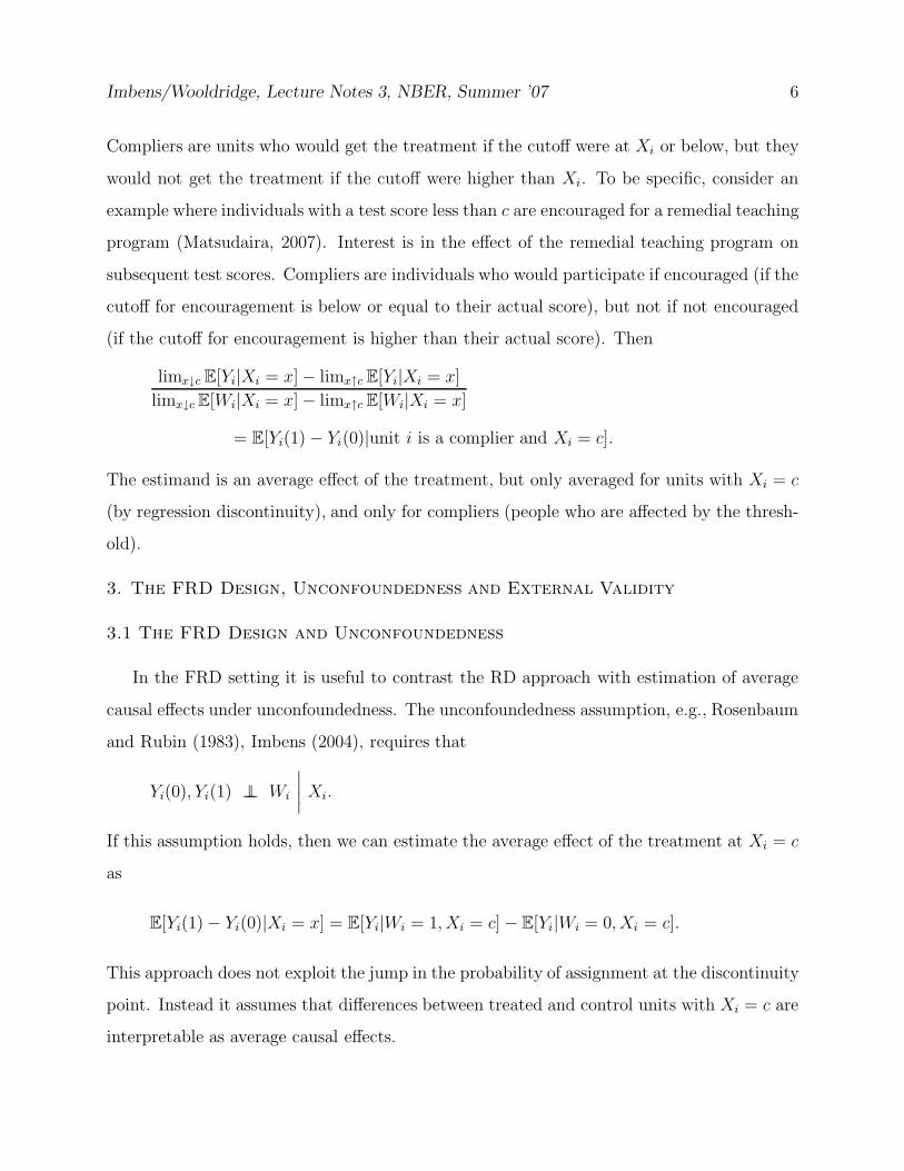
Imbens/Wooldridge, Lecture Notes 3, NBER, Summer ’07 6
Compliers are units who would get the treatment if the cutoff were at Xi or below, but they
would not get the treatment if the cutoff were higher than Xi. To be specific, consider an
example where individuals with a test score less than c are encouraged for a remedial teaching
program (Matsudaira, 2007). Interest is in the effect of the remedial teaching program on
subsequent test scores. Compliers are individuals who would participate if encouraged (if the
cutoff for encouragement is below or equal to their actual score), but not if not encouraged
(if the cutoff for encouragement is higher than their actual score). Then
limx↓c E[Yi|Xi = x] − limx↑c E[Yi|Xi = x]
limx↓c E[Wi|Xi = x] − limx↑c E[Wi|Xi = x]
= E[Yi(1) − Yi(0)|unit i is a complier and Xi = c].
The estimand is an average effect of the treatment, but only averaged for units with Xi = c
(by regression discontinuity), and only for compliers (people who are affected by the thresh-
old).
3. The FRD Design, Unconfoundedness and External Validity
3.1 The FRD Design and Unconfoundedness
In the FRD setting it is useful to contrast the RD approach with estimation of average
causal effects under unconfoundedness. The unconfoundedness assumption, e.g., Rosenbaum
and Rubin (1983), Imbens (2004), requires that
Yi(0), Yi(1) ⊥⊥ Wi
∣
∣
∣
∣
Xi.
If this assumption holds, then we can estimate the average effect of the treatment at Xi = c
as
E[Yi(1) − Yi(0)|Xi = x] = E[Yi|Wi = 1, Xi = c] − E[Yi|Wi = 0, Xi = c].
This approach does not exploit the jump in the probability of assignment at the discontinuity
point. Instead it assumes that differences between treated and control units with Xi = c are
interpretable as average causal effects.
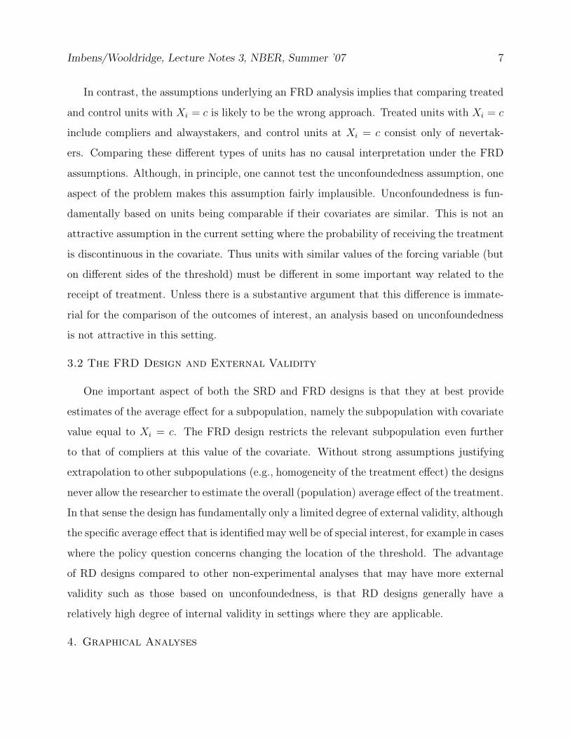
Imbens/Wooldridge, Lecture Notes 3, NBER, Summer ’07 7
In contrast, the assumptions underlying an FRD analysis implies that comparing treated
and control units with Xi = c is likely to be the wrong approach. Treated units with Xi = c
include compliers and alwaystakers, and control units at Xi = c consist only of nevertak-
ers. Comparing these different types of units has no causal interpretation under the FRD
assumptions. Although, in principle, one cannot test the unconfoundedness assumption, one
aspect of the problem makes this assumption fairly implausible. Unconfoundedness is fun-
damentally based on units being comparable if their covariates are similar. This is not an
attractive assumption in the current setting where the probability of receiving the treatment
is discontinuous in the covariate. Thus units with similar values of the forcing variable (but
on different sides of the threshold) must be different in some important way related to the
receipt of treatment. Unless there is a substantive argument that this difference is immate-
rial for the comparison of the outcomes of interest, an analysis based on unconfoundedness
is not attractive in this setting.
3.2 The FRD Design and External Validity
One important aspect of both the SRD and FRD designs is that they at best provide
estimates of the average effect for a subpopulation, namely the subpopulation with covariate
value equal to Xi = c. The FRD design restricts the relevant subpopulation even further
to that of compliers at this value of the covariate. Without strong assumptions justifying
extrapolation to other subpopulations (e.g., homogeneity of the treatment effect) the designs
never allow the researcher to estimate the overall (population) average effect of the treatment.
In that sense the design has fundamentally only a limited degree of external validity, although
the specific average effect that is identified may well be of special interest, for example in cases
where the policy question concerns changing the location of the threshold. The advantage
of RD designs compared to other non-experimental analyses that may have more external
validity such as those based on unconfoundedness, is that RD designs generally have a
relatively high degree of internal validity in settings where they are applicable.
4. Graphical Analyses
Imbens/Wooldridge, Lecture Notes 3, NBER, Summer ’07 8
4.1 Introduction
Graphical analyses should be an integral part of any RD analysis. The nature of RD
designs suggests that the effect of the treatment of interest can be measured by the value of
the discontinuity in the expected value of the outcome at a particular point. Inspecting the
estimated version of this conditional expectation is a simple yet powerful way to visualize
the identification strategy. Moreover, to assess the credibility of the RD strategy, it is useful
to inspect two additional graphs. The estimators we discuss later use more sophisticated
methods for smoothing but these basic plots will convey much of the intuition. For strikingly
clear examples of such plots, see Lee, Moretti, and Butler (2004), Lalive (2007), and Lee
(2007). Two figures from Lee (2007) are attached.
4.2 Outcomes by Forcing Variable
The first plot is a histogram-type estimate of the average value of the outcome by the
forcing variable. For some binwidth h, and for some number of bins K0 and K1 to the left and
right of the cutoff value, respectively, construct bins (bk, bk+1], for k = 1, . . . , K = K0 + K1,
where
bk = c − (K0 − k + 1) · h.
Then calculate the number of observations in each bin,
Nk =
N∑
i=1
1bk < Xi ≤ bk+1,
and the average outcome in the bin:
Y k =1
Nk·
N∑
i=1
Yi · 1bk < Xi ≤ bk+1.
The first plot of interest is that of the Y k, for k = 1, K against the mid point of the bins,
bk = (bk + bk+1)/2. The question is whether around the threshold c there is any evidence of
a jump in the conditional mean of the outcome. The formal statistical analyses discussed
below are essentially just sophisticated versions of this, and if the basic plot does not show
Imbens/Wooldridge, Lecture Notes 3, NBER, Summer ’07 9
any evidence of a discontinuity, there is relatively little chance that the more sophisticated
analyses will lead to robust and credible estimates with statistically and substantially sig-
nificant magnitudes. In addition to inspecting whether there is a jump at this value of the
covariate, one should inspect the graph to see whether there are any other jumps in the con-
ditional expectation of Yi given Xi that are comparable to, or larger than, the discontinuity
at the cutoff value. If so, and if one cannot explain such jumps on substantive grounds, it
would call into question the interpretation of the jump at the threshold as the causal effect
of the treatment. In order to optimize the visual clarity it is important to calculate averages
that are not smoothed over the cutoff point. The attached figure is taken from the paper by
Lee (2007).
4.2 Covariates by Forcing Variable
The second set of plots compares average values of other covariates in the K bins. Specifi-
cally, let Zi be the M-vector of additional covariates, with m-th element Zim. Then calculate
Zkm =1
Nk·
N∑
i=1
Zim · 1bk < Xi ≤ bk+1.
The second plot of interest is that of the Zkm, for k = 1, K against the mid point of the
bins, bk, for all m = 1, . . . , M . Lee (2007) presents such a figure for a lagged value of the
outcome, namely the election results from a prior election, against the vote share in the last
election. In the case of FRD designs, it is also particularly useful to plot the mean values of
the treatment variable Wi to make sure there is indeed a jump in the probability of treatment
at the cutoff point. Plotting other covariates is also useful for detecting possible specification
problems (see Section 8) in the case of either SRD or FRD designs.
4.3 The Density of the Forcing Variable
In the third graph one should plot the number of observations in each bin, Nk, against
the mid points bk. This plot can be used to inspect whether there is a discontinuity in the
distribution of the forcing variable X at the threshold. McCrary (2007) suggests that such
discontinuity would raise the question whether the value of this covariate was manipulated
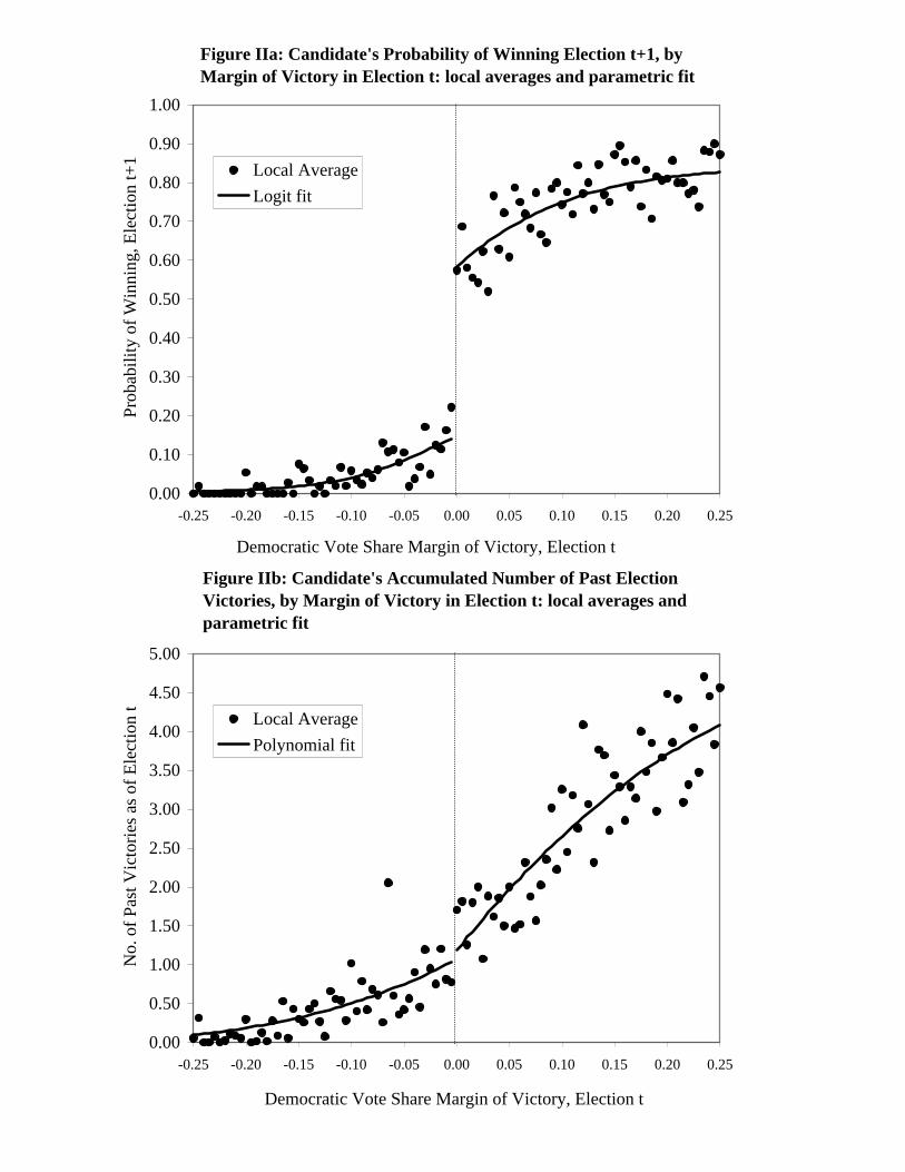
0.00
0.10
0.20
0.30
0.40
0.50
0.60
0.70
0.80
0.90
1.00
-0.25 -0.20 -0.15 -0.10 -0.05 0.00 0.05 0.10 0.15 0.20 0.25
Local AverageLogit fit
Democratic Vote Share Margin of Victory, Election t
Prob
abili
ty o
f Win
ning
, Ele
ctio
n t+
1
Figure IIa: Candidate's Probability of Winning Election t+1, by Margin of Victory in Election t: local averages and parametric fit
0.00
0.50
1.00
1.50
2.00
2.50
3.00
3.50
4.00
4.50
5.00
-0.25 -0.20 -0.15 -0.10 -0.05 0.00 0.05 0.10 0.15 0.20 0.25
Local AveragePolynomial fit
No.
of P
ast V
icto
ries a
s of E
lect
ion
t
Figure IIb: Candidate's Accumulated Number of Past Election Victories, by Margin of Victory in Election t: local averages and parametric fit
Democratic Vote Share Margin of Victory, Election t

Imbens/Wooldridge, Lecture Notes 3, NBER, Summer ’07 10
by the individual agents, invalidating the design. For example, suppose that the forcing
variable is a test score. If individuals know the threshold and have the option of re-taking
the test, individuals with test scores just below the threshold may do so, and invalidate the
design. Such a situation would lead to a discontinuity of the conditional density of the test
score at the threshold, and thus be detectable in plots such as described here. See Section 8
for more discussion of the specification tests based on this idea.
5. Estimation: Local Linear Regression
5.1 Nonparametric Regression at the Boundary
The practical estimation of the treatment effect τ in both the SRD and FRD designs
is largely standard nonparametric regression (e.g., Pagan and Ullah, 1999; Hardle, 1990;
Li and Racine, 2007). However, there are two unusual features to estimation in the RD
setting. First, we are interested in the regression function at a single point, and second, that
single point is a boundary point. As a result, standard nonparametric kernel regression does
not work very well. At boundary points, such estimators have a slower rate of convergence
than they do at interior points. Standard methods for choosing the bandwidth are also not
designed to provide good choices in this setting.
5.2 Local Linear Regression
Here we discuss local linear regression (Fan and Gijbels, 1996). Instead of locally fitting a
constant function, we can fit linear regression functions to the observations within a distance
h on either side of the discontinuity point:
minαl,βl
N∑
i|c−h<Xi<c
(Yi − αl − βl · (Xi − c))2 ,
and
minαr,βr
N∑
i|c≤Xi<c+h
(Yi − αr − βr · (Xi − c))2 .
The value of µl(c) and µr(c) are then estimated as
µl(c) = αl + βl · (c − c) = αl, and µr(c) = αr + βr · (c − c) = αr,
Imbens/Wooldridge, Lecture Notes 3, NBER, Summer ’07 11
Given these estimates, the average treatment effect is estimated as
τSRD = αr − αl.
Alternatively one can estimate the average effect directly in a single regression, by solving
minα,β,τ,γ
N∑
i=1
1c − h ≤ Xi ≤ c + h · (Yi − α − β · (Xi − c) − τ · Wi − γ · (Xi − c) ·Wi)2 ,
which will numerically yield the same estimate of τSRD.
We can make the nonparametric regression more sophisticated by using weights that
decrease smoothly as the distance to the cutoff point increases, instead of the zero/one
weights based on the rectangular kernel. However, even in this simple case the asymptotic
bias can be shown to be of order h2, and the more sophisticated kernels rarely make much
difference. Furthermore, if using different weights from a more sophisticated kernel does
make a difference, it likely suggests that the results are highly sensitive to the choice of
bandwidth. So the only case where more sophisticated kernels may make a difference is
when the estimates are not very credible anyway because of too much sensitivity to the
choice of bandwidth. From a practical point of view one may just focus on the simple
rectangular kernel, but verify the robustness of the results to different choices of bandwidth.
For inference we can use standard least squares methods. Under appropriate conditions
on the rate at which the bandwidth goes to zero as the sample size increases, the resulting
estimates will be asymptotically normally distributed, and the (robust) standard errors from
least squares theory will be justified. Using the results from HTV, the optimal bandwidth is
h ∝ N−1/5. Under this sequence of bandwidths the asymptotic distribution of the estimator
τ will have a non-zero bias. If one does some undersmoothing, by requiring that h ∝ N−δ
with 1/5 < δ < 2/5, then the asymptotic bias disappears and standard least squares variance
estimators will lead to valid confidence intervals.
5.3 Covariates
Often there are additional covariates available in addition to the forcing covariate that
is the basis of the assignment mechanism. These covariates can be used to eliminate small
Imbens/Wooldridge, Lecture Notes 3, NBER, Summer ’07 12
sample biases present in the basic specification, and improve the precision. In addition,
they can be useful for evaluating the plausibility of the identification strategy, as discussed
in Section 8.1. Let the additional vector of covariates be denoted by Zi. We make three
observations on the role of these additional covariates.
The first and most important point is that the presence of these covariates rarely changes
the identification strategy. Typically, the conditional distribution of the covariates Z given X
is continuous at x = c. If such discontinuities in other covariates are found, the justification
of the identification strategy may be questionable. If the conditional distribution of Z given
X is continuous at x = c, then including Z in the regression
minα,β,τ,δ
N∑
i=1
1c−h ≤ Xi ≤ c+h·(Yi − α − β · (Xi − c) − τ ·Wi − γ · (Xi − c) · Wi − δ′Zi)2,
will have little effect on the expected value of the estimator for τ , since conditional on X
being close to c, the additional covariates Z are independent of W .
The second point is that even though with X very close to c, the presence of Z in the
regression does not affect any bias, in practice we often include observations with values of
X not too close to c. In that case, including additional covariates may eliminate some bias
that is the result of the inclusion of these additional observations.
Third, the presence of the covariates can improve precision if Z is correlated with the
potential outcomes. This is the standard argument, which also supports the inclusion of
covariates even in analyses of randomized experiments. In practice the variance reduction
will be relatively small unless the contribution to the R2 from the additional regressors is
substantial.
5.4 Estimation for the Fuzzy Regression Discontinuity Design
In the FRD design, we need to estimate the ratio of two differences. The estimation issues
we discussed earlier in the case of the SRD arise now for both differences. In particular,
there are substantial biases if we do simple kernel regressions. Instead, it is again likely to
be better to use local linear regression. We use a uniform (rectangular) kernel, with the same
Imbens/Wooldridge, Lecture Notes 3, NBER, Summer ’07 13
bandwidth for estimation of the discontinuity in the outcome and treatment regressions.
First, consider local linear regression for the outcome, on both sides of the discontinuity
point. Let
(
αyl, βyl
)
= arg minαyl,βyl
∑
i:c−h≤Xi<c
(Yi − αyl − βyl · (Xi − c))2 , (3)
(
αyr, βyr
)
= arg minαyr,βyr
∑
i:c≤Xi≤c+h
(Yi − αyr − βyr · (Xi − c))2. (4)
The magnitude of the discontinuity in the outcome regression is then estimated as τy =
αyr − αyl. Second, consider the two local linear regression for the treatment indicator:
(
αwl, βwl
)
= arg minαwl,βwl
∑
i:c−h≤Xi<c
(Wi − αwl − βwl · (Xi − c))2 , (5)
(
αwr, βwr
)
= arg minαwr,βwr
∑
i:c≤Xi≤c+h
(Yi − αwr − βwr · (Xi − c))2 . (6)
The magnitude of the discontinuity in the treatment regression is then estimated as τw =
αwr − αwl. Finally, we estimate the effect of interest as the ratio of the two discontinuities:
τFRD =τy
τw=
αyr − αyl
αwr − αwl. (7)
Because of the specific implementation we use here, with a uniform kernel, and the same
bandwidth for estimation of the denominator and the numerator, we can characterize the
estimator for τ as a Two-Stage-Least-Squares (TSLS) estimator (See HTV). This equality
still holds when we use local linear regression and include additional regressors. Define
Vi =
11Xi < c · (Xi − c)1Xi ≥ c · (Xi − c)
, and δ =
αyl
βyl
βyr
. (8)
Then we can write
Yi = δ′Vi + τ · Wi + εi. (9)
Estimating τ based on the regression function (9) by TSLS methods, with the indicator
1Xi ≥ c as the excluded instrument and Vi as the set of exogenous variables is numerically
identical to τFRD as given in (7).
Imbens/Wooldridge, Lecture Notes 3, NBER, Summer ’07 14
6. Bandwidth Selection
An important issue in practice is the selection of the smoothing parameter, the binwidth
h. Here we focus on cross-validation procedures rather than plug in methods which would
require estimating derivatives nonparametrically. The specific methods discussed here are
based on those developed by Ludwig and Miller (2005, 2007). Initially we focus on the SRD
case, and in Section 6.2 we extend the recommendations to the FRD setting.
To set up the bandwidth choice problem we generalize the notation slightly. In the SRD
setting we are interested in the
τSRD = limx↓c
µ(x) − limx↑c
µ(x),
where µ(x) = E[Yi|Xi = x]. We estimate the two terms as
limx↓c
µ(x) = αr(c), and limx↑c
µ(x) = αl(c),
where αl(x) and βl(x) solve
(
αl(x), βl(x))
= arg minα,β
∑
j|x−h<Xj<x
(Yj − α − β · (Xj − x))2 . (10)
and αr(x) and βr(x) solve
(
αr(x), βr(x))
= arg minα,β
∑
j|x<Xj<x+h
(Yj − α − β · (Xj − x))2 . (11)
Let us focus first on estimating limx↓c µ(x). For estimation of this limit we are interested in
the bandwidth h that minimizes
Qr(x, h) = E
[
(
limz↓x
µ(z) − αr(x)
)2]
,
at x = c. However, we focus on a single bandwidth for both sides of the threshold, and
therefore focus on minimizing
Q(c, h) =1
2·(Ql(c, h) + Qr(c, h)) =
1
2·(
E
[
(
limx↑c
µ(x) − αl(c)
)2]
+ E
[
(
limx↓c
µ(x) − αr(c)
)2])
.
Imbens/Wooldridge, Lecture Notes 3, NBER, Summer ’07 15
We now discuss two methods for choosing the bandwidth.
6.1 Bandwidth Selection for the SRD Design
For a given binwidth h, let the estimated regression function at x be
µ(x) =
αl(x) if x < c,αr(x) if x ≥ c,
where αl(x), βl(x), αr(x) and βr(x) solve (10) and (11). Note that in order to mimic the
fact that we are interested in estimation at the boundary we only use the observations on
one side of x in order to estimate the regression function at x, rather than the observations
on both sides of x, that is, observations with x − h < Xj < x + h. In addition, the strict
inequality in the definition implies that µ(x) evaluated at x = Xi does not depend on Yi.
Now define the cross-validation criterion as
CVY (h) =1
N
N∑
i=1
(Yi − µ(Xi))2 , (12)
with the corresponding cross-validation choice for the binwidth
hoptCV = arg min
hCVY (h).
The expected value of this cross-validation function is under some conditions equal to
E[CVY (h)] = C + E[Q(X, h)] = C +∫
Q(x, h)fX(dx), for some constant that does not
depend on h. Although the modification to estimate the regression using one-sided kernels
mimics more closely the estimand of interest, this is still not quite what we are interested
in. Ultimately we are solely interested in estimating the regression function in the neigh-
borhood of a single point, the threshold c, and thus in minimizing Q(c, h), rather than∫
xQ(x, h)fX(x)dx. If there are few observations in the tails of the distributions, minimizing
the criterion in (12) may lead to larger bins than is optimal for estimating the regression
function around x = c if c is in the center of the distribution. We may therefore wish to
minimize the cross-validation criterion after first discarding observations from the tails. Let
qX,δ,l be δ quantile of the empirical distribution of X for the subsample with Xi < c, and let
Imbens/Wooldridge, Lecture Notes 3, NBER, Summer ’07 16
qX,δ,r be δ quantile of the empirical distribution of X for the subsample with Xi ≥ c. Then
we may wish to use the criterion
CVδY (h) =
1
N
∑
i:qX,δ,l≤Xi≤qX,1−δ,r
(Yi − µ(Xi))2 . (13)
The modified cross-validation choice for the bandwidth is
hδ,optCV = arg min
hCVδ
Y (h). (14)
The modified cross-validation function has expectation, again ignoring terms that do not
involve h, proportional to E[Q(X, h)|qX,δ,l < X < qX,δ,r]. Choosing a smaller value of δ
makes the expected value of the criterion closer to what we are ultimately interested, that is,
Q(c, h), but has the disadvantage of leading to a noisier estimate of E[CVδY (h)]. In practice
one may wish to choose δ = 1/2, and discard 50% of the observations on either side of the
threshold, and afterwards assess the sensitivity of the bandwidth choice to the choice of δ.
Ludwig and Miller (2005) implement this by using only data within 5 percentage points of
the threshold on either side.
6.2 Bandwidth Selection for the FRD Design
In the FRD design, there are four regression functions that need to be estimated: the
expected outcome given the forcing variable, both on the left and right of the cutoff point,
and the expected value of the treatment, again on the left and right of the cutoff point. In
principle, we can use different binwidths for each of the four nonparametric regressions.
In the section on the SRD design, we argued in favor of using identical bandwidths for
the regressions on both sides of the cutoff point. The argument is not so clear for the pairs of
regressions functions by outcome we have here, and so in principle we have two optimal band-
widths, one based on minimizing CVδY (h), and one based on minimizing CVδ
W (h), defined
correspondingly. It is likely that the conditional expectation of the treatment is relatively
flat compared to the conditional expectation of the outcome variable, suggesting one should
use a larger binwidth for estimating the former.5 Nevertheless, in practice it is appealing
5In the extreme case of the SRD design the conditional expectation of W given X is flat on both sides
Imbens/Wooldridge, Lecture Notes 3, NBER, Summer ’07 17
to use the same binwidth for numerator and denominator. Since typically the size of the
discontinuity is much more marked in the expected value of the treatment, one option is to
use the optimal bandwidth based on the outcome discontinuity. Alternatively, to minimize
bias, one may wish to use the smallest bandwidths selected by the cross validation criterion
applied separately to the outcome and treatment regression:
hoptCV = min
(
arg minh
CVδY (h), arg min
hCVδ
W (h))
,
where CVδY (h) is as defined in (12), and CVδ
W (h) is defined similarly. Again a value of
δ = 1/2 is likely to lead to reasonable estimates in many settings.
7. Inference
We now discuss some asymptotic properties for the estimator for the FRD case given
in (7) or its alternative representation in (9).6 More general results are given in HTV. We
continue to make some simplifying assumptions. First, as in the previous sections, we use a
uniform kernel. Second, we use the same bandwidth for the estimator for the jump in the
conditional expectations of the outcome and treatment. Third, we undersmooth, so that
the square of the bias vanishes faster than the variance, and we can ignore the bias in the
construction of confidence intervals. Fourth, we continue to use the local linear estimator.
Under these assumptions we give an explicit expression for the asymptotic variance, and
present two estimators for the asymptotic variance. The first estimator follows explicitly the
analytic form for the asymptotic variance, and substitutes estimates for the unknown quanti-
ties. The second estimator is the standard robust variance for the Two-Stage-Least-Squares
(TSLS) estimator, based on the sample obtained by discarding observations when the forcing
covariate is more than h away from the cutoff point. Both are robust to heteroskedasticity.
7.1 The Asymptotic Variance
To characterize the asymptotic variance we need a couple of additional pieces of notation.
of the threshold, and so the optimal bandwidth would be infinity. Therefore, in practice it is likely that theoptimal bandwidth would be larger for estimating the jump in the conditional expectation of the treatmentthan in estimating the jump in the conditional expectation of the outcome.
6The results for the SRD design are a special case of these for the FRD design.
Imbens/Wooldridge, Lecture Notes 3, NBER, Summer ’07 18
Define the four variances
σ2Y l = lim
x↑cVar(Yi|Xi = x), σ2
Y r = limx↓c
Var(Yi|Xi = x),
σ2Wl = lim
x↑cVar(Wi|Xi = x), σ2
Wr = limx↓c
Var(Wi|Xi = x),
and the two covariances
CY Wl = limx↑c
Cov(Yi, Wi|Xi = x), CY Wr = limx↓c
Cov(Yi, Wi|Xi = x).
Note that because of the binary nature of W , it follows that σ2Wl = µWl · (1 − µWl), where
µWl = limx↑c Pr(Wi = 1|Xi = x), and similarly for σ2Wr. To discuss the asymptotic variance
of τ it is useful to break it up in three pieces. The asymptotic variance of√
Nh(τy − τy) is
Vτy =4
fX(c)·(
σ2Y r + σ2
Y l
)
. (15)
The asymptotic variance of√
Nh(τw − τw) is
Vτw =4
fX(c)·(
σ2Wr + σ2
Wl
)
(16)
The asymptotic covariance of√
Nh(τy − τy) and√
Nh(τw − τw) is
Cτy,τw =4
fX(c)· (CY Wr + CY Wl) . (17)
Finally, the asymptotic distribution has the form
√Nh · (τ − τ )
d−→ N(
0,1
τ 2w
· Vτy +τ 2y
τ 4w
· Vτw − 2 · τy
τ 3w
· Cτy,τw
)
. (18)
This asymptotic distribution is a special case of that in HTV (page 208), using the rectangular
kernel, and with h = N−δ, for 1/5 < δ < 2/5 (so that the asymptotic bias can be ignored).
7.2 A Plug-in Estimator for the Asymptotic Variance
We now discuss two estimators for the asymptotic variance of τ . First, we can estimate
the asymptotic variance of τ by estimating each of the components, τw, τy, Vτw , Vτy , and
Cτy,τw and substituting them into the expression for the variance in (18). In order to do this
we first estimate the residuals
εi = Yi − µy(Xi) = Yi − 1Xi < c · αyl − 1Xi ≥ c · αyr ,
Imbens/Wooldridge, Lecture Notes 3, NBER, Summer ’07 19
ηi = Wi − µw(Xi) = Wi − 1Xi < c · αwl − 1Xi ≥ c · αwr.
Then we estimate the variances and covariances consistently as
σ2Y l =
1
Nhl
∑
i|c−h≤Xi<c
ε2i , σ2
Y r =1
Nhr
∑
i|c≤Xi≤c+h
ε2i ,
σ2Wl =
1
Nhl
∑
i|c−h≤Xi<c
η2i , σ2
Wr =1
Nhr
∑
i|c≤Xi≤c+h
η2i ,
CY Wl =1
Nhl
∑
i|c−h≤Xi<c
εi · ηi, CY Wr =1
Nhr
∑
i|c≤Xi≤c+h
εi · ηi.
Finally, we estimate the density consistently as
fX(x) =Nhl + Nhr
2 · N · h .
Then we can plug in the estimated components of Vτy , VτW, and CτY ,τW
from (15)-(17), and
finally substitute these into the variance expression in (18).
7.3 The TSLS Variance Estimator
The second estimator for the asymptotic variance of τ exploits the interpretation of the τ
as a TSLS estimator, given in (9). The variance estimator is equal to the robust variance for
TSLS based on the subsample of observations with c − h ≤ Xi ≤ c + h, using the indicator
1Xi ≥ c as the excluded instrument, the treatment Wi as the endogenous regressor and
the Vi defined in (8) as the exogenous covariates.
8. Specification Testing
There are generally two main conceptual concerns in the application of RD designs,
sharp or fuzzy. A first concern about RD designs is the possibility of other changes at the
same cutoff value of the covariate. Such changes may affect the outcome, and these effects
may be attributed erroneously to the treatment of interest. The second concern is that of
manipulation of the covariate value.
8.1 Tests Involving Covariates

Imbens/Wooldridge, Lecture Notes 3, NBER, Summer ’07 20
One category of tests involves testing the null hypothesis of a zero average effect on pseudo
outcomes known not to be affected by the treatment. Such variables includes covariates that
are by definition not affected by the treatment. Such tests are familiar from settings with
identification based on unconfoundedness assumptions. In most cases, the reason for the
discontinuity in the probability of the treatment does not suggest a discontinuity in the
average value of covariates. If we find such a discontinuity, it typically casts doubt on the
assumptions underlying the RD design. See the second part of the Lee (2007) figure for an
example.
8.2 Tests of Continuity of the Density
The second test is conceptually somewhat different, and unique to the RD setting. Mc-
Crary (2007) suggests testing the null hypothesis of continuity of the density of the covariate
that underlies the assignment at the discontinuity point, against the alternative of a jump
in the density function at that point. Again, in principle, one does not need continuity of
the density of X at c, but a discontinuity is suggestive of violations of the no-manipulation
assumption. If in fact individuals partly manage to manipulate the value of X in order to be
on one side of the boundary rather than the other, one might expect to see a discontinuity
in this density at the discontinuity point.
8.3 Testing for Jumps at Non-discontinuity Points
Taking the subsample with Xi < c we can test for a jump in the conditional mean of the
outcome at the median of the forcing variable. To implement the test, use the same method
for selecting the binwidth as before. Also estimate the standard errors of the jump and use
this to test the hypothesis of a zero jump. Repeat this using the subsample to the right
of the cutoff point with Xi ≥ c. Now estimate the jump in the regression function and at
qX,1/2,r, and test whether it is equal to zero.
8.4 RD Designs with Misspecification
Lee and Card (2007) study the case where the forcing variable variable X is discrete. In
practice this is of course always true. This implies that ultimately one relies for identification

Imbens/Wooldridge, Lecture Notes 3, NBER, Summer ’07 21
on functional form assumptions for the regression function µ(x). Lee and Card consider a
parametric specification for the regression function that does not fully saturate the model,
that is, it has fewer free parameters than there are support points. They then interpret the
deviation between the true conditional expectation E[Y |X = x] and the estimated regression
function as random specification error that introduces a group structure on the standard er-
rors. Lee and Card then show how to incorporate this group structure into the standard
errors for the estimated treatment effect. Within the local linear regression framework dis-
cussed in the current paper one can calculate the Lee-Card standard errors (possibly based
on slightly coarsened covariate data if X is close to continuous) and compare them to the
conventional ones.
8.5 Sensitivity to the Choice of Bandwidth
One should investigate the sensitivity of the inferences to this choice, for example, by
including results for bandwidths twice (or four times) and half (or a quarter of) the size of
the originally chosen bandwidth. Obviously, such bandwidth choices affect both estimates
and standard errors, but if the results are critically dependent on a particular bandwidth
choice, they are clearly less credible than if they are robust to such variation in bandwidths.
8.6 Comparisons to Estimates Based on Unconfoundedness in the FRD Design
If we have an FRD design, we can also consider estimates based on unconfoundedness.
Inspecting such estimates and especially their variation over the range of the covariate can
be useful. If we find that for a range of values of X, our estimate of the average effect of the
treatment is relatively constant and similar to that based on the FRD approach, one would
be more confident in both sets of estimates.
Imbens/Wooldridge, Lecture Notes 3, NBER, Summer ’07 22
References
Angrist, J.D., G.W. Imbens and D.B. Rubin (1996), “Identification of Causal
Effects Using Instrumental Variables,” Journal of the American Statistical Association, 91,
444-472.
Angrist, J.D. and A.B. Krueger, (1991), Does Compulsory School Attendance
Affect Schooling and Earnings?, Quarterly Journal of Economics 106, 979-1014.
Angrist, J.D., and V. Lavy, (1999), Using Maimonides’ Rule to Estimate the Effect
of Class Size on Scholastic Achievement”, Quarterly Journal of Economics 114, 533-575.
Black, S., (1999), Do Better Schools Matter? Parental Valuation of Elementary Edu-
cation, Quarterly Journal of Economics 114, 577-599.
Card, D., A. Mas, and J. Rothstein, (2006), Tipping and the Dynamics of Segre-
gation in Neighborhoods and Schools, Unpublished Manuscript, Department of Economics,
Princeton University.
Chay, K., and M. Greenstone, (2005), Does Air Quality Matter; Evidence from the
Housing Market, Journal of Political Economy 113, 376-424.
Cook, T., (2007), “Waiting for Life to Arrive”: A History of the Regression-Discontinuity
Design in Psychology, Statistics, and Economics, forthcoming, Journal of Econometrics.
DiNardo, J., and D.S. Lee, (2004), Economic Impacts of New Unionization on Private
Sector Employers: 1984-2001, Quarterly Journal of Economics 119, 1383-1441.
Fan, J. and I. Gijbels, (1996), Local Polynomial Modelling and Its Applications (Chap-
man and Hall, London).
Hahn, J., P. Todd and W. Van der Klaauw, (2001), Identification and Estimation
of Treatment Effects with a Regression Discontinuity Design, Econometrica 69, 201-209.
Hardle, W., (1990), Applied Nonparametric Regression (Cambridge University Press,
New York).
Imbens/Wooldridge, Lecture Notes 3, NBER, Summer ’07 23
Imbens, G., and J. Angrist (1994), “Identification and Estimation of Local Average
Treatment Effects,” Econometrica, Vol. 61, No. 2, 467-476.
Imbens, G., and T. Lemieux, (2007) “Regression Discontinuity Designs: A Guide to
Practice,” forthcoming, Journal of Econometrics.
Lee, D.S. and D. Card, (2007), Regression Discontinuity Inference with Specification
Error, forthcoming, Journal of Econometrics.
Lee, D.S., Moretti, E., and M. Butler, (2004), Do Voters Affect or Elect Policies?
Evidence from the U.S. House, Quarterly Journal of Economics 119, 807-859.
Lemieux, T. and K. Milligan, (2007), Incentive Effects of Social Assistance: A
Regression Discontinuity Approach, forthcoming, Journal of Econometrics.
Ludwig, J., and D. Miller, (2005), Does Head Start Improve Children’s Life Chances?
Evidence from a Regression Discontinuity Design, NBER working paper 11702.
McCrary, J., (2007), Testing for Manipulation of the Running Variable in the Regres-
sion Discontinuity Design, forthcoming, Journal of Econometrics.
McEwan, P., and J. Shapiro, (2007),The Benefits of Delayed Primary School En-
rollment: Discontinuity Estimates using exact Birth Dates,” Unpublished manuscript.
Pagan, A. and A. Ullah, (1999), Nonparametric Econometrics, Cambridge University
Press, New York.
Porter, J., (2003), Estimation in the Regression Discontinuity Model,” mimeo, Depart-
ment of Economics, University of Wisconsin, http://www.ssc.wisc.edu/ jporter/reg discont 2003.pdf.
Shadish, W., T. Campbell and D. Cook, (2002), Experimental and Quasi-experimental
Designs for Generalized Causal Inference (Houghton Mifflin, Boston).
Thistlewaite, D., and D. Campbell, (1960), Regression-Discontinuity Analysis:
An Alternative to the Ex-Post Facto Experiment, Journal of Educational Psychology 51,
309-317.
Imbens/Wooldridge, Lecture Notes 3, NBER, Summer ’07 24
Trochim, W., (1984), Research Design for Program Evaluation; The Regression-discontinuity
Design (Sage Publications, Beverly Hills, CA).
Trochim, W., (2001), Regression-Discontinuity Design, in N.J. Smelser and P.B Baltes,
eds., International Encyclopedia of the Social and Behavioral Sciences 19 (Elsevier North-
Holland, Amsterdam) 12940-12945.
Van Der Klaauw, W., (2002), Estimating the Effect of Financial Aid Offers on College
Enrollment: A Regression–discontinuity Approach, International Economic Review 43, 1249-
1287.
Imbens/Wooldridge, Lecture Notes 4, Summer ’07
What’s New in Econometrics? NBER, Summer 2007Lecture 4, Monday, July 30th, 3.15-4.15 pm
Nonlinear Panel Data ModelsThese notes summarize some recent, and perhaps not-so-recent, advances in the estimation
of nonlinear panel data models. Research in the last 10 to 15 years has branched off in twodirections. In one, the focus has been on parameter estimation, possibly only up to a commonscale factor, in semiparametric models with unobserved effects (that can be arbitrarilycorrelated with covariates.) Another branch has focused on estimating partial effects whenrestrictions are made on the distribution of heterogeneity conditional on the history of thecovariates. These notes attempt to lay out the pros and cons of each approach, payingparticular attention to the tradeoff in assumptions and the quantities that can be estimated.1. Basic Issues and Quantities of Interest
Most microeconomic panel data sets are best characterized as having few time periods and(relatively) many cross section observations. Therefore, most of the discussion in these notesassumes T is fixed in the asymptotic analysis while N is increasing. We assume random samplein the cross section, xit,yit : t 1, . . . ,T. Take yit to be a scalar for simplicity. If we are notconcerned about traditional (contemporaneous) endogeneity, then we are typically interested in
Dyit|xit,c i (1.1)
or some feature of this distribution, such as Eyit|xit,c i, or a conditional median. In the case ofa mean, how do we summarize the partial effects? Let mtxt,c be the mean function. If xtj is
continuous, then
jxt,c ≡∂mtxt,c∂xtj
, (1.2)
or look at discrete changes. How do we account for unobserved ci? If we want to estimatemagnitudes of effects, we need to know enough about the distribution of c i so that we caninsert meaningful values for c. For example, if c Ec i, then we can compute the partial
effect at the average (PEA),
jxt,c. (1.3)
Of course, we need to estimate the function mt and the mean of ci. If we know more about thedistribution of c i, we can insert different quantiles, for example, or a certain number ofstandard deviations from the mean.
Alternatively, we can average the partial effects across the distribution of ci:
1
Imbens/Wooldridge, Lecture Notes 4, Summer ’07
APExt Eci jxt,c i. (1.4)
The difference between (1.3) and (1.4) can be nontrivial for nonlinear mean functions. Thedefinition in (1.4) dates back at least to Chamberlain (1982), and is closely related to the notionof the average structural function (ASF) (Blundell and Powell (2003)). The ASF is defined as
ASFxt Ecimtxt,c i. (1.5)
Assuming the derivative passes through the expectation results in (1.5), the average partialeffect. Of course, computing discrete changes gives the same result always. APEs are directlyacross models, and APEs in general nonlinear models are comparable to the estimatedcoefficients in a standard linear model.
Semiparametric methods, which, by construction, are silent about the distribution of c i,unconditionally or conditional on xi1, . . . ,xiT, cannot generally deliver estimates of averagepartial (marginal) effects. Instead, an index structure is usually imposed so that parameters canbe consistently estimated. So, for example, with scalar heterogeneity we might have an indexmodel with additive heterogeneity:
mtxt,c Gxt c, (1.6)
where, say, G is strictly increasing and continuously differentiable (and, in some cases, isknown, and in others, is not). Then
jxt,c jgxt c, (1.7)
where g is the derivative of G. Then estimating j means we can estimate the sign of the
partial effect, and even the relative effects of any two continuous variables. But, even if G isspecified (the more common case), the magnitude of the effect evidently cannot be estimatedwithout making assumptions about the distribution of ci: the size of the scale factor for arandom draw i, gxt ci, depends on ci. Without knowing something about the distributionof ci we cannot generally locate gxt ci.
Returning to the general case, Altonji and Matzkin (2005) focus on what they call the localaverage response (LAR) as opposed to the APE or PAE. The LAR at xt for a continuousvariable xtj is
∂mtxt,c∂xtj
dHtc|xt, (1.8)
where Htc|xt denotes the cdf of Dc i|xit xt. This is a “local” partial effect because itaverages out the heterogeneity for the slice of the population given by the vector xt. The APE,
2
Imbens/Wooldridge, Lecture Notes 4, Summer ’07
which by comparison could be called a “global average response,” averages out over the entiredistribution of c i. See also Florens, Heckman, Meghir, and Vytlacil (2004).
It is important to see that the definitions of partial effects does not depend on the nature ofthe variables in xt (except for whether it makes sense to use the calculus approximation or usechanges). In particular, xt can include lagged dependent variables and lags of other variables,which may or may not be strictly exogenous. Unfortunately, we cannot identify the APEs, oreven relative effects in index models, without some assumptions.2. Exogeneity Assumptions on the Covariates
Ideally, we would only have to specify a model for Dyit|xit,c i or some feature.Unfortunately, it is well known that specifying a full parametric model is not sufficient foridentifying either the parameters of the model or the partial effects defined in Section 1. In thissection, we consider two useful exogeneity assumptions on the covariates.
It is easiest to deal with estimation under a strict exogeneity assumption. The most usefuldefinition of strict exogeneity for nonlinear panel data models is
Dyit|xi1, . . . ,xiT,c i Dyit|xit,c i, (2.1)
which means that xir, r ≠ t, does not appear in the conditional distribution of yit once xit and c i
have been counted for. Chamberlain (1984) labeled (2.1) strict exogeneity conditional on theunobserved (or latent) effects c i. Sometimes, a conditional mean version is sufficient:
Eyit|xi1, . . . ,xiT,c i Eyit|xit,ci, (2.2)
which we already saw for linear models. (In other cases a condition stated in terms ofconditional medians is more convenient.) Of course, either version of the assumption rules outlagged dependent variables, but also other situations where there may be feedback fromidiosyncratic changes in yit to future movements in xir, r t. But it is the assumptionunderlying the most common estimation methods for nonlinear models.
More natural is a sequential exogeneity assumption (conditional on the unobserved effects)assumption, which we can state generally as
Dyit|xi1, . . . ,xit,c i Dyit|xit,ci (2.3)
or, sometimes, in terms of specific features of the distribution. Assumption (2.3) allows forlagged dependent variables and does not restrict feedback. Unfortunately, it is much moredifficult to allow, especially in nonlinear models.
Neither (2.2) nor (2.3) allows for contemporaneous endogeneity of one or more elements of
3
Imbens/Wooldridge, Lecture Notes 4, Summer ’07
xit, where, say, xitj is correlated with unobserved, time-varying unobservables that affect yit, or
where xitj is simultaneously determined along with yit. This will be covered in later notes on
control function methods.3. Conditional Independence Assumption
In some cases – certainly traditionally – a conditional independence assumption isimposed. We can write the condition generally as
Dyi1, . . . ,yiT|xi,c i t1
T
Dyit|xi,c i. (3.1)
This assumption is only useful in the context of the strict exogeneity assumption (2.1), inwhich case we can write
Dyi1, . . . ,yiT|xi,c i t1
T
Dyit|xit,c i. (3.2)
In a parametric context, the conditional independence assumption therefore reduces our task tospecifying a model for Dyit|xit,c i, and then determining how to treat the unobservedheterogeneity, c i. In random effects and CRE frameworks, conditional independence plays acritical role in being able to estimate the parameters in distribution the of c i. We could get bywith less restrictive assumptions by parameterizing the dependence, but that increasescomputational burden. As it turns out, conditional independence plays no role in estimatingAPEs for a broad class of models. (That is, we do not need to place restrictions onDyi1, . . . ,yiT|xi,c i. Before we can study estimation, we must discuss the critical issue of thedependence between c i and xi.4. Assumptions about the Unobserved Heterogeneity
The modern approach to panel data analysis with micro data treats the unobservedheterogeneity as random draws along with the observed data, and that is the view taken here.Nevertheless, there are still reasons one might treat them as parameters to estimate, and weallow for that in our discussion.
Random EffectsFor general nonlinear models, what we call the “random effects” assumption is
independence between c i and xi xi1, . . . ,xiT:
Dc i|xi1, . . . ,xiT Dc i. (4.1)
4
Imbens/Wooldridge, Lecture Notes 4, Summer ’07
If we combine this assumption with a model for mtxt,c, then the APEs are actuallynonparametrically identified. (And, in fact, we do not need to assume strict or sequentialexogeneity to use a pooled estimation method, or to use just a single time period.) In fact, ifEyit|xit,c i mtxit,c i and Dc i|xit Dc i, then the APEs are obtained from
rtxt ≡ Eyit|xit xt. (4.2)
(The argument is a simple application of the law of interated expectations; it is discussed indetail in Wooldridge (2005a).) In principle, Eyit|xit can be estimated nonparametrically, andwe only need a single time period to identify the partial effects for that time period.
In some leading cases (for example random effects probit and Tobit with heterogeneitynormally distributed), if we want to obtain partial effects for different values of c, we mustassume more: the strict exogeneity assumption (2.1), the conditional independence assumption(3.1), and the random effects assumption (4.1) with a parametric distribution for Dc i aretypically sufficient. We postpone this discussion because it takes us into the realm ofspecifying parametric models.
Correlated Random EffectsA “correlated random effects” framework allows dependence between c i and xi, but the
dependence in restricted in some way. In a parametric setting, we specify a distribution forDc i|xi1, . . . ,xiT, as in Mundlak (1978), Chamberlain (1982), and many subsequent authors.For many models, including probit and Tobit, one can allow Dc i|xi1, . . . ,xiT to depend in a“nonexchangeable” manner on the time series of the covariates; Chamberlain’s random effectsprobit model does this. But the distributional assumptions that lead to simple estimation –namely, homoskedastic normal with a linear conditional mean — are restrictive. But it is aslopossible to assume
Dci|xi Dci|xi (4.3)
without specifying Dci|xi or restricting any feature of this distribution. We will see in thenext section that (4.3) is very powerful.
We can go further. For example, suppose that we think the heterogeneity c i is correlatedwith features of the covariates other than just the time average. Altonji and Matzkin (2005)allow for xi in equation (4.3) to be replaced by other functions of xit : t 1, . . . ,T, such assample variances and covariance. These are examples of “exchangeable” functions ofxit : t 1, . . . ,T – that is, statistics whose value is the same regardless of the ordering of the
5
Imbens/Wooldridge, Lecture Notes 4, Summer ’07
xit. Non-exchangeable functions can be used, too. For example, we might think that ci iscorrelated with individual-specific trends, and so we obtain wi as the intercept and slope fromthe unit-specific regressions xit on 1, t, t 1, . . . ,T (for T ≥ 3); we can also add the errorvariance from this individual specific regression if we have sufficient time periods. Then, thecondition becomes
Dci|xi Dci|wi. (4.4)
Practically, we need to specify wi and then establish that there is enough variation inxit : t 1, . . . ,T separate from wi; this will be clear in the next section.
Fixed EffectsUnfortunately, the label “fixed effects” is used in different ways by different researchers
(and, sometimes, by the same researcher). The traditional view was that a fixed effectsframework meant c i, i 1, . . . ,N were treated as parameters to estimate. This view is stillaround, and, when researchers say they estimated a nonlinear panel data model by “fixedeffects,” they sometimes mean the c i were treated as parameters to estimate along with otherparameters (whose dimension does not change with N). As is well known, except in specialcases, estimation of the c i generally introduces an “incidental parameters” problem. (More onthis later when we discuss estimation methods, and partial effects.) Subject to computationalfeasilibity, the approach that treats the ci as parameters is widely applicable.
The “fixed effects” label can mean that Dci|xi is unrestricted. Even in that case, there aredifferent approaches to estimation of parameters. One is to specify a joint distributionDyi1, . . . ,yit|xi,c i such that a sufficient statistic, say si, can be found such that
Dyi1, . . . ,yit|xi,c i, si Dyi1, . . . ,yit|xi, si, (4.5)
and where the latter distribution still depends on the parameters of interest in a way thatidentifies them. In most cases, the conditional independence assumption (3.1) is maintained,although one CMLE is known to have robustness properties: the so-called “fixed effects”Poisson estimator. We cover that later on.5. Nonparametric Identification of Average Partial and LocalAverage Effects
Before considering identification and estimation of parameters in parametric models, it isuseful to ask which quantities, if any, are identified without imposing parametric assumptions.Not surprisingly, there are no known results on nonparametric identificiation of partial effects
6
Imbens/Wooldridge, Lecture Notes 4, Summer ’07
evaluated at specific values of c, such as c – except, of course, when the partial effects do not
depend on c. Interestingly, identification can fail even under a full set of strong parametricassumptions. For example, in the probit model
Py 1|x,c x c, (5.1)
where x is 1 K an includes unity, the partial effect for a continuous variable xj is simply
jx c. The partial effect at the mean of c is simply jx. Suppose we assume that c|x
~Normal0,c2. Then it is easy to show that
Py 1|x x/1 c21/2, (5.2)
which means that only the scaled parameter vector c ≡ /1 c21/2 is identified. Therefore,
jx, is evidently unidentified. (The fact that probit of y on x estimates c has been called
the “attenuation bias” that results from omitted variables in the context of probit, even whenthe omitted variable is independent of the covariates and normally distributed. As mentionedearlier more generally, the average partial effects are obtained directly from Py 1|x, and, infact, are given by cjxc. As discussed in Wooldridge (2002, Chapter 15), cjxc can be
larger or smaller in magnitude than the PEA jx: |cj|≤ |j| but xc ≥ x.
A related example is due to Hahn (2001), and is related to the nonidentification restuls ofChamberlain (1993). Suppose that xit is a binary indicator (for example, a policy variable).Consider the unobserved effects probit model
Pyit 1|xi,ci xit ci, (5.3)
As discussed by Hahn, is not known to be identified in this model, even under conditionalserial independence assumption and the random effects assumption Dci|xi Dci. But theaverage partial effect, which in this case is an average treatment effect, is simply ≡ E ci − Eci. By the general result cited earlier, is consistently estimated (infact, unbiasedly estimated) by using a difference of means for the treated and untreated groups,for either time period. In fact, as discussed in Wooldridge (2005a), identification of the APEholds if we replace with an unknown function G and allow Dci|xi Dci|xi. But theparameters are still not identified.
To summarize: the APE is identified for any function G whether or not the conditionalserial independence holds, even if we add separate year intercepts. But is not identified underthe strongest set of assumptions. This simple example suggests that perhaps our focus onparameters is wrong-headed.
7
Imbens/Wooldridge, Lecture Notes 4, Summer ’07
We can establish identification of average partial effects much more generally. Assumeonly that the strict exogeneity assumption (2.1) holds along with Dci|xi Dci|xi. Thesetwo assumptions are sufficient to identify the APEs. To see why, note that the averagestructural function at time t can be written as
ASFtxt Ecimtxt,c i E xiEmtxt,c i|xi ≡ E xirtxt, xi, (5.4)
where rtxt, xi ≡ Ertxt,c i|xi. It follows that, given an estimator rt, of the functionrt, , the ASF can be estimated as
ASFtxt ≡ N−1∑i1
N
rtxt, xi, (5.5)
and then we can take derivatives or changes with respect to the entries in xt. Notice that (5.4)holds without the strict exogeneity assumption (2.1) or the assumption Dci|xi Dci|xi.However, these assumptions come into play in our ability to estimate rt, . If we combine(21) and (4.3) we have
Eyit|xi EEyit|xi,c i|xi Emtxit,c i|xi mtxit,cdFc|xi
mtxit,cdFc|xi rtxit, xi, (5.6)
where Fc|xi denotes the cdf of Dc i|xi (which can be a discrete, continuous, or mixeddistribution), the second equality follows from (2.1), the fourth equality follows fromassumption (4.3), and the last equality folllows from the definition of rt, Of course,because Eyit|xi depends only on xit, xi, we must have
Eyit|xit, xi rtxit, xi. (5.7)
Further, xit : t 1, . . . ,T is assumed to have time variation, and so xit and xi can be used asseparate regressors even in a fully nonparametric setting.
Altonji and Matskin (2005).use this idea more generally, and focus on estimating the localaverage response. Wooldridge (2005a) used Dc i|xi Dc i|xi generally in the case xit isdiscrete, in which case a full nonparametric analysis is easy. When
Dci|xi Dc i|wi (5.8)
for wi a function of xi, Altonji and Matzkin (2005) show that the LAR can be obtained as
∂rtxt,w∂xtj
dKtw|xt, (5.9)
8
Imbens/Wooldridge, Lecture Notes 4, Summer ’07
where rxt,w Eyit|xit xt,wi w and Ktw|xt is the cdf of Dwi|xit xt. Altonji andMatskin demonstrate how to estimate the LAR based on nonparametric estimation ofEyit|xit,wi followed by “local” averaging, that is, averaging ∂ryit|xt,wi/∂xtj over
observations i with xit “close” to xt.This analysis demonstrates that APEs are nonparametrically identified under the
conditional mean version of strict exogeneity, (2.1), and (5.8), at least for time-varyingcovariates if wi is restricted in some way. In fact, we can identify the APEs for a single timeperiod with just one year of data on y. We only need to obtain xi and, in effect, include it as acontrol. Of course, efficiency would be gained by assuming some stationarity across t andusing a pooled method.6. Dynamic Models
General models with only sequentially exogenous variables are difficult to deal with.Arellano and Carrasco (2003) consider probit models. Wooldridge (2000) suggests a strategythe requires modeling the dynamic distribution of the variables that are not strictly exogenous.Much more is known about models with lagged dependent variables and otherwise strictlyexogenous variables. So, we start with a model for
Dyit|zit,yi,t−1, . . . ,zi1,yi0,c i, t 1, . . . ,T, (6.1)
which we assume also is Dyit|zi,yi,t−1, . . . ,yi1,yi0,c i where zi is the entire history
zit : t 1, . . . ,T. This is the sense in which the zit are strictly exogenous.Suppose this model depends only on zit,yi,t−1,ci, so ftyt|zt,yt−1,c;. The joint density of
yi1, . . . ,yiT given yi0,zi,c i is
t1
T
ftyt|zt,yt−1,c;. (6.2)
The problem with using this for estimation is the presence of c i along with the initial condition,yi0. Approaches: (i) Treat the c i as parameters to estimate (incidental parameters problem,
although recent research has attempted to reduce the asymptotic bias in the partial effects). (ii)Try to estimate the parameters without specifying conditional or unconditional distributions forci. (Available in some special cases covered below, but other restrictions are needed. And,generally, cannot estimate partial effects.). (iii) Find or, more practically, approximateDyi0|c i, zi and then model Dc i|zi. After integrating out ci we obtain the density for
Dyi0,yi1, . . . ,yiT|zi and we can use MLE (conditional on zi), (iv) Model Dc i|yi0,zi. After
9
Imbens/Wooldridge, Lecture Notes 4, Summer ’07
integrating out ci we obtain the density for Dyi1, . . . ,yiT|yi0,zi, and we can use MLE
(conditional on yi0,zi). As shown by Wooldridge (2005b), in some leading cases – probit,
ordered probit, Tobit, Poisson regression – there is a density hc|y0,z that mixes with the
density fy1, . . . ,yT|y0,z,c to produce a log-likelihood that is in a common family and carried
out by standard software.If mtxt,c, is the mean function Eyt|xt,c for a scalar yt, then average partial effects are
easy to obtain. The average structural function is
ASFxt Ecimtxt,c i, E mtxt,c,hc|yi0,zi,dc |yi0,zi . (6.3)
The term inside the brackets, say rtxt,yi0, zi,, is available, at least in principle, becausemt and h have been specified. Often, they have simple forms, in fact. Generally, it can besimulated. In any case, ASFxt, is consistently estimated by
ASFxt N−1∑t1
T
rtxt,yi0,zi, , .
Partial derivatives and differences with respect to elements of xt (which, remember, caninclude yt−1) can be computed. With large N and small T, the panel data bootstrap can be usedfor standard errors and inference.7. Applications to Specific Models
We now turn to some common parametric models and highlight the difference betweenestimation partial effects at different values of the heterogeneity and estimating average partialeffects. An analysis of Tobit models follows in a very similar way to those in the followingtwo sections. See Wooldridge (2002, Chapter 16) and Honoré and Hu (2004).
7.1 Binary and “Fractional” Response Models
We start with the standard specification for the unobserved effects (UE) probit model,which is
Pyit 1|xit,ci xit ci, t 1, . . . ,T, (7.1)
where xit does not contain an overall intercept but would usually include time dummies. Wecannot identify or the APEs without further assumptions. The traditional RE probit modelsimposes a strong set of assumptions: strict exogeneity, conditional serial independence, andindependence between ci and xi with ci ~Normalc,c
2. Under these assumptions, and theparameters in the distribution of ci are identified and are consistently estimated by full MLE
10
Imbens/Wooldridge, Lecture Notes 4, Summer ’07
(conditional on xi.We can relax independence between ci and xi using the Chamberlain-Mundlak device
under conditional normality:
ci xi ai,ai|xi ~Normal0,a2, (7.2)
where the time average is often used to save on degrees of freedom. We can relax (7.2) andallow Chamberlain’s (1980) more flexible device:
ci xi ai xi11 . . .xiTT ai (7.3)
Even when the r seem to be very different, the Mundlak restriction can deliver similar
estimates of the other parameters and the APEs. (In the linear case, they both produce the usualFE estimator of .
If we still assume conditional serial independence then all parameters are identified. We
can estimate the mean of ci as c N−1∑ i1N xi and the variance as
c2 ≡
′ N−1∑ i1N xi
′xi a2. Of course, ci is not generally normally distributed unless xi is.
The approximation might get better as T gets large. In any case, we can plug in values of c thatare a certain number of estimated standard deviations from c, say c c.
The APEs are identified from the ASF, which is consistently estimated as
ASFxt N−1∑i1
N
xta a xia (7.4)
where, for example, a /1 a21/2. The derivatives or changes of ASFxt with respect to
elements of xt can be compared with fixed effects estimates from a linear model. Often, if wealso average out across xit, the linear FE estimates are similar to the averaged effects.
As we discussed generally in Section 5, the APEs are defined without the conditional serial
independence assumption. Without Dyi1, . . . ,yiT|xi,ci t1
T
Dyit|xit,ci, we can still estimate
the scaled parameters because
Pyit 1|xi xita a xia, (7.5)
and so pooled probit consistently estimates the scaled parametes. (Time dummies have beensupressed for simplicity.) Now we have direct estimates of a, a, and a, and we insert those
directly into (7.4).Using pooled probit can be inefficient for estimating the scaled parameters, whereas the
11
Imbens/Wooldridge, Lecture Notes 4, Summer ’07
full MLE is efficient but not (evidently) robust to violation of the conditional serialindependence assumption. It is possible to estimate the parameters more efficiently than pooledprobit that is still consistent under the same set of assumptions. One possibility is minimumdistance estimation. That is, estimate a separate models for each t, and then impose therestrictions using minimum distance methods. (This can be done with or without the Mundlakdevice.)
A different approach is to apply the so called “generalized estimating equations” (GEE)approach. Briefly, GEE applied to panel data is essentially weighted multivariate nonlinearleast squares (WMNLS) with explicit recognition that the weighting matrix might not be theinverse of the conditional variance matrix. In most nonlinear panel data models, obtaining theactual matrix Varyi|xi is difficult, if not impossible, because integrating out the heterogeneity
does not deliver a closed form. The GEE approach uses Varyit|xi implied by the specificdistribution – in the probit case, we have the correct conditional variances,
Varyit|xi xita a xia1 − xita a xia ≡ vit. (7.6)
The “working” correlation matrix oftenusually specified as “exchangeable,”
Correit,eis|xi “ ”, (7.7)
where eit yit − xita a xiavit1/2 is the standardized error. Or, each pair t, s is
allowed to have its own correlation but which is assumed to be independent of x i
(“unstructured”). The conditional correlation Correit,eis|xi is not constant, but that is theworking assumption. The hope is to improve efficiency over the pooled probit estimator whilemaintaining the robustness of the pooled estimator. (The full RE probit estimator is not robustto serial dependence.) A robust sandwich matrix is easily computed provided the conditionalmean function (in this case, response probability) is correctly specified.
Because the Bernoulli log-likelihood is in the linear exponential family (LEF), exactly thesame methods can be applied if 0 ≤ yit ≤ 1 – that is, yit is a “fractional” response – but wherethe model is for the conditional mean: Eyit|xit,ci xit ci. Pooled “probit” or minimumdistance estimation or GEE can be used. Now, however, we must make inference robust toVaryit|xit, xi not having the probit form. (There are cases where Varyit|xit, xi is proportionalto (7.6), and so it still makes sense to use the probit quasi-log-likelihood. Pooled nonlinearregression is another possibility or weighted multivariate nonlinear regression are also possibleand a special case of GEE.)
12
Imbens/Wooldridge, Lecture Notes 4, Summer ’07
A more radical suggestion, but in the spirit of Altonji and Matzkin (2005) and Wooldridge(2005a), is to just use a flexible model for Eyit|xit, xidirectly. For example, if yit is binary, ora fractional response, 0 ≤ yit ≤ 1, we might just specify a flexible parametric model, such as
Eyit|xit, xi t xit xi xi ⊗ xi xit ⊗ xi, (7.8)
or the “heteroskedastic probit” model
Eyit|xit, xi t xit xiexp−xi. (7.9)
If we write either of these functions as rtxt, x then the average structural function is estimated
as ASFtxt ≡ N−1∑ i1N rtxt, xi, where the “^” indicates that we have substituted in the
parameter estimates. We can let all parameters depend on t, or we can estimate the parametersseparately for each t and then use minimum distance estimation to impose the parameterrestrictions. The justification for using, say, (7.8) is that we are interested in the average partialeffects, and how parameters appear is really not the issue. Even though (7.8) cannot be derivedfrom Eyit|xit,ci xit ci or any other standard model, there is nothing sacred about thisformulation. In fact, it is fairly simplistic. We can view (7.8) as the approximation to the trueEyit|xit, xi obtained after integrating ci out of the unknown function mxt,ci. (We couldformalize this process by using series estimation, as in Newey (1988), where the number ofterms is allowed to grow with N.) This is the same argument used by, say, Angrist (2001) injustifying linear models for limited dependent variables when the focus on primarily onaverage effects.
The argument is essentially unchanged if we replace xi with other statistics wi. Forexample, we might run, for each i, the regression xit on 1, t, t 1, . . . ,T and use the interceptand slope (on the time trend) as the elements of wi. Or, we can use sample variances andcovariances for each i, along with the sample mean. Or, we can use initial values and averagegrowth rates. The key condition is Dc i|xi Dc i|wi, and then we need sufficient variationin xit : t 1, . . . ,T not explained by wi for identification. (Naturally, as we expand wi, thenumber of time periods required generally increases.)
Of course, once we just view (7.8) as an approximation, we can are justified in using thelogistic function, say
Eyit|xit, xi t xit xi xi ⊗ xi xit ⊗ xi, (7.10)
where z expz/1 expz, which, again, can be applied to binary or fractionalresponses. The focus on partial effects that average out the heterogeneity can be liberating in
13

Imbens/Wooldridge, Lecture Notes 4, Summer ’07
that it means the step of specifying Eyit|xit,c i is largely superfluous, and, in fact, can get inthe way of pursuing a suitably flexible analysis. On the other hand, if we start with, say, a“structural” model such as Pyi1 1|xi,c i ai xitbi, which is a heterogeneous indexmodel, then we cannot derive equations such as (7.8) or (7.9), even under the strongassumption that c i is independent of xi and multivariate normal. If we imposed theChamberlain device for the elements of c i we can get expressions “close” to a combination of(7.8) and (7.9). Whether one is willing to simply estimate relative simple models such as (7.8)in order to estimate APEs depends on one’s taste for bypassing more traditional formulations.
If we start with the logit formulation
Pyit 1|xit,ci xit ci, (7.11)
then we can estimate the parameters, without restricting Dci|xi in any way, but we mustadd the conditional independence assumption. (No one has been able to show that, unlike inthe linear model, or the Poisson model covered below, that the MLE that conditions on the
number of successes ni ∑ t1T yit is robust to serial dependence. It appears not to be. Plus, the
binary nature of yit appears to be critical, so the conditional MLE cannot be applied tofractional responses even under serial independence.) Because we have not restricted Dci|xi
in any way, it appears that we cannot estimate average partial effects. As commonly happens innonlinear models, if we relax assumptions about the distribution of heterogeneity, we lose theability to estimate partial effects. We can estimate the effects of the covariates on the log-oddsratio, and relative partial effects of continuous variables. But for partial effects themselves, wedo not have sensible values to plug in for c, and we cannot average across its distribution.
The following table summarizes the features of various approaches to estimating binaryresponse unobserved effects models.
14
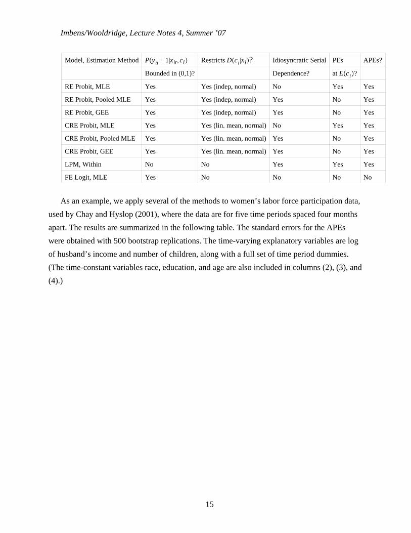
Imbens/Wooldridge, Lecture Notes 4, Summer ’07
Model, Estimation Method Pyit 1|xit,ci Restricts Dci |xi? Idiosyncratic Serial PEs APEs?
Bounded in (0,1)? Dependence? at Eci?
RE Probit, MLE Yes Yes (indep, normal) No Yes Yes
RE Probit, Pooled MLE Yes Yes (indep, normal) Yes No Yes
RE Probit, GEE Yes Yes (indep, normal) Yes No Yes
CRE Probit, MLE Yes Yes (lin. mean, normal) No Yes Yes
CRE Probit, Pooled MLE Yes Yes (lin. mean, normal) Yes No Yes
CRE Probit, GEE Yes Yes (lin. mean, normal) Yes No Yes
LPM, Within No No Yes Yes Yes
FE Logit, MLE Yes No No No No
As an example, we apply several of the methods to women’s labor force participation data,used by Chay and Hyslop (2001), where the data are for five time periods spaced four monthsapart. The results are summarized in the following table. The standard errors for the APEswere obtained with 500 bootstrap replications. The time-varying explanatory variables are logof husband’s income and number of children, along with a full set of time period dummies.(The time-constant variables race, education, and age are also included in columns (2), (3), and(4).)
15
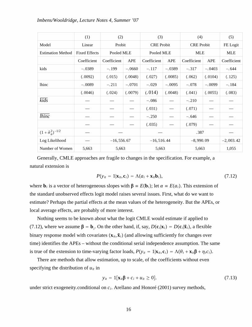
Imbens/Wooldridge, Lecture Notes 4, Summer ’07
(1) (2) (3) (4) (5)
Model Linear Probit CRE Probit CRE Probit FE Logit
Estimation Method Fixed Effects Pooled MLE Pooled MLE MLE MLE
Coefficient Coefficient APE Coefficient APE Coefficient APE Coefficient
kids −. 0389 −. 199 −. 0660 −. 117 −. 0389 −. 317 −. 0403 −. 644
. 0092 . 015 . 0048 . 027 . 0085 . 062 . 0104 . 125
lhinc −. 0089 −. 211 −. 0701 −. 029 −. 0095 −. 078 −. 0099 −. 184
. 0046 . 024 . 0079 (. 014 . 0048 . 041 . 0055 . 083
kids — — — −. 086 — −. 210 — —
— — — . 031 — . 071 — —
lhinc — — — −. 250 — −. 646 — —
— — — . 035 — . 079 — —
1 a2−1/2 — — — . 387 —
Log Likelihood — −16, 556. 67 −16, 516. 44 −8, 990. 09 −2, 003. 42
Number of Women 5,663 5,663 5,663 5,663 1,055
Generally, CMLE approaches are fragile to changes in the specification. For example, anatural extension is
Pyit 1|xit,c i ai xitbi, (7.12)
where bi is a vector of heterogeneous slopes with ≡ Ebi; let ≡ Eai. This extension ofthe standard unobserved effects logit model raises several issues. First, what do we want toestimate? Perhaps the partial effects at the mean values of the heterogeneity. But the APEs, orlocal average effects, are probably of more interest.
Nothing seems to be known about what the logit CMLE would estimate if applied to(7.12), where we assume bi. On the other hand, if, say, Dc i|xi Dc i|xi, a flexible
binary response model with covariates xit, xi (and allowing sufficiently for changes overtime) identifies the APEs – without the conditional serial independence assumption. The sameis true of the extension to time-varying factor loads, Pyit 1|xit,c i t xit tci.
There are methods that allow estimation, up to scale, of the coefficients without evenspecifying the distribution of uit in
yit 1xit ci uit ≥ 0. (7.13)
under strict exogeneity.conditional on ci. Arellano and Honoré (2001) survey methods,
16
Imbens/Wooldridge, Lecture Notes 4, Summer ’07
including variations on Manski’s maximum score estimator.Estimation of parameters and APEs is much more difficult even in simple dynamic models.
Consider
Pyit 1|zi,yi,t−1, . . . ,yi0,ci Pyit 1|zit,yi,t−1,ci, t 1, . . . ,T,
which combines correct dynamic specification with strict exogeneity of zit. For a dynamicprobit model
Pyit 1|zit,yi,t−1,ci zit yi,t−1 ci. (7.14)
Treating the ci as parameters to estimate causes inconsistency in and (although there isrecent work by Woutersen and Fernández-Val that shows how to make the asymptotic bias oforder 1/T2; see the next section). A simple analysis is available if we specify
ci|zi,yi0 Normal 0yi0 zi,a2 (7.15)
Then
Pyit 1|zi,yi,t−1, . . . ,yi0,ai zit yi,t−1 0yi0 zi ai, (7.16)
where ai ≡ ci − − 0yi0 − zi. Because ai is independent of yi0,zi, it turns out we can usestandard random effects probit software, with explanatory variables 1,zit,yi,t−1,yi0,zi in timeperiod t. Easily get the average partial effects, too:
ASFzt,yt−1 N−1∑i1
N
zta ayt−1 a a0yi0 zia, (7.17)
and take differences or derivatives with respect to elements of zt,yt−1. As before, thecoefficients are multiplied by 1 a
2−1/2. Of course, both the structural model and model forDci|yi0,zi can be made more flexible (such as including interactions, or letting Varci|zi,yi0
be heteroskedastic).We apply this method to the Chay and Hyslop data and estimate a model for
Plfpit 1|kidsit, lhincit, lfpi,t−1,ci, where one lag of labor force participation is assumed tosuffice for the dynamics and kidsit, lhincit : t 1, . . . ,T is assumed to be strictlyexogenous conditional on ci. Also, we include the time-constant variables educ, black, age,and age2 and a full set of time-period dummies. (We start with five periods and lose one withthe lag. Therefore, we estimate the model using four years of data.) We include among theregressors the initial value, lfpi0, kidsi1 through kidsi4, and lhinci1 through lhinci4. Estimatingthe model by RE probit gives 1.541 se . 067, and so, even after controlling for
17
Imbens/Wooldridge, Lecture Notes 4, Summer ’07
unobserved heterogeneity, there is strong evidence of state dependence. But to obtain the sizeof the effect, we compute the APE for lfpt−1. The calculation involves averaging
zita a a0yi0 zia − zita a0yi0 zia across all t and i; we must be sure to
scale the original coefficients by 1 a2−1/2, where, in this application, a
2 1.103. The APEestimated from this method is about .259. In other words, averaged across all women and alltime periods, the probability of being in the labor force at time t is about .26 higher if thewomen was in the labor force at time t − 1 than if she was not. This estimate controls forunobserved heterogeneity, number of young children, husband’s income, and the woman’seducation, race, and age.
It is instructive to compare the APE with the estimate of a dynamic probit model thatignores ci. In this case, we just use pooled probit of lfpit on1,kidsit, lhincit, lfpi,t−1educi,blacki,agei, and agei
2 and include a full set of period dummies.The coefficient on lfpi,t−1 is 2.876 (se . 027, which is much higher than in the dynamic REprobit model. More importantly, the APE for state dependence is about .837, which is muchhigher than when heterogeneity is controlled for. Therefore, in this example, much of thepersistence in labor force participation of married women is accounted for by the unobservedheterogeneity. There is still some state dependence, but its value is much smaller than a simpledynamic probit indicates.
Arellano and Carrasco (2003) use a different approach to estimate the parameters andAPEs in dynamic binary response models with only sequentially exogenous variables. Thus,their method applies to models with lagged dependent variables, but also other models wherethere made be feedback from past shocks to future covariates. (Their assumptions essentiallyimpose serial conditional serial independence.) Rather than impose an assumption such as(7.15), they use a different approximation. Let vit ci uit be the composed error inyit 1xit ci uit ≥ 0. Then, in the context of a probit model, they assume
vit|wit ~NormalEci|wit, t2 (7.18)
where wit xit,yi,t−1,xi,t−1, . . . ,yi1xi1. The mean Eci|wit is unrestricted (although, of course,they are linked across time by interacted expectations because wit ⊂ wi,t1, but the shape ofthe distribution is assumed to be the same across t. Arellano and Carrasco discuss identificationand estimation, and extensions to models with time-varying factor loads.
Honoré and Kyriazidou (2000) extend an idea of Chamberlain’s and show how to estimate and in a logit model without distributional assumptions for ci. They find conditional
18
Imbens/Wooldridge, Lecture Notes 4, Summer ’07
probabilities that do not depend on ci but still depend on and . However, in the case withfour time periods, t 0,1,2, and 3, the conditioning that removes ci requires zi2 zi3. HKshow how to use a local version of this condition to consistenty estimate the parameters. Theestimator is also asymptotically normal, but converges more slowly than the usual N -rate.
The condition that zi2 − zi3 have a distribution with support around zero rules out aggregateyear dummies or even linear time trends. Plus, using only observations with zi2 − zi3 in aneighborhood of zero results in much lost data. Finally, estimates of partial effects or averagepartial effects are not available.
While semiparametric approaches can be valuable to comparing parameter estimates withmore parametric approaches, such comparisons have limitations. For example, the coefficientson yt−1 in the dynamic logit model and the dynamic probit model are comparable only in sign;we cannot take the derivative with respect to yt−1 because it is discrete. Because we do notknow where the evaluate the partial effects – that is, the values of c to plug in, or average outacross the distribution of ci, we cannot compare the magnitudes with CRC approaches. We cancompare the relative effects on the continuous elements in zt based on partial derivatives. Buteven here, if we find a difference between semiparametric and parametric methods, is itbecause aggregate time effects were excluded in the semiparametric estimation or because themodel of Dci|yi0,zi was misspecified? Currently, we have no good ways of deciding.(Recently, Li and Zheng (2006) use Bayesian methods to estimate a dynamic Tobit model withunobserved heterogeneity, where they distribution of unosberved heterogeneity is an infinitemixture of normals. They find that all of the average partial effects are very similar to thoseobtained from the much simpler specification in (7.15).)
Honoré and Lewbel (2002) show how to estimate in the model
yit 1vit xit ci uit ≥ 0 (7.19)
without distributional assumptions on ci uit. The special continuous explanatory variable vit,which need not be time varying, is assumed to appear in the equation (and its coefficient isnormalized to one). More importantly, vit is assumed to satisfyDci uit|vit,xit, zi Dci uit|xit, zi, which is a conditional independence assumption. Thevector zi is assumed to be independent of uit in all time periods. (So, if two time periods areused, zi could be functions of variables determined prior to the earliest time period.) The mostlikely scenario is when vit is randomized and therefore independent of xit, zi,eit, whereeit ci uit. It seems unlikely to hold if vit is related to past outcomes on yit. The estimator
19
Imbens/Wooldridge, Lecture Notes 4, Summer ’07
derived by Honoré and Lewbel is N -asymptotically normal, and fairly easy to compute; itrequires estimation of the density of vit given xit, ziand then a simple IV estimation.
Honoré and Tamer (2006) have recently shown how to obtain bounds on parameters andAPEs in dynamic models, including the dynamic probit model; these are covered in the noteson partial identification.
7.2 Count and Other Multiplicative Models
Several options are available for models with conditional means multiplicative in theheterogeneity. The most common is
Eyit|xit,ci ci expxit (7.20)
where ci ≥ 0 is the unobserved effect and xit would incude a full set of year dummies in mostcases. First consider estimation under strict exogeneity (conditional on ci):
Eyit|xi1, . . . ,xiT,ci Eyit|xit,ci. (7.21)
If we add independence between ci and xi – a random effects approach – then, using Eci 1as a normalization,
Eyit|xi expxit, (7.22)
and various estimation methods can be used to account for the serial dependence in yit ifonly xi is conditioned on. (Serial correlation is certainly present because of ci, but it could bepresent due to idiosyncratic shocks, too.) Regardless of the actual distribution of yit, or even itsnature – other than yit ≥ 0 – the pooled Poisson quasi-MLE is consistent for under (7.22) butlikely very inefficient; robust inference is straightforward with small T and large N.
Random effects Poisson requires that Dyit|xi,ci has a Poisson distribution with mean(7.20), and maintains the conditional independence assumption,
Dyi1, . . . ,yiT|xi,ci t1
T
Dyit|xit,ci,
along with a specific distribution for ci – usually a Gamma distribution with unit mean.Unfortunately, like RE probit, the full MLE has no known robustness properties. The Poissondistribution needs to hold along with the other assumptions. A generalized estimating approachis available, too. If the Poisson quasi-likelihood is used, the GEE estimator is fully robustprovided the mean is correctly specified. One can use an exchangeable, or at least constant,working correlation matrix. See Wooldridge (2002, Chapter 19).
A CRE model can be allowed by writing ci exp xiai where ai is independent of xi
20
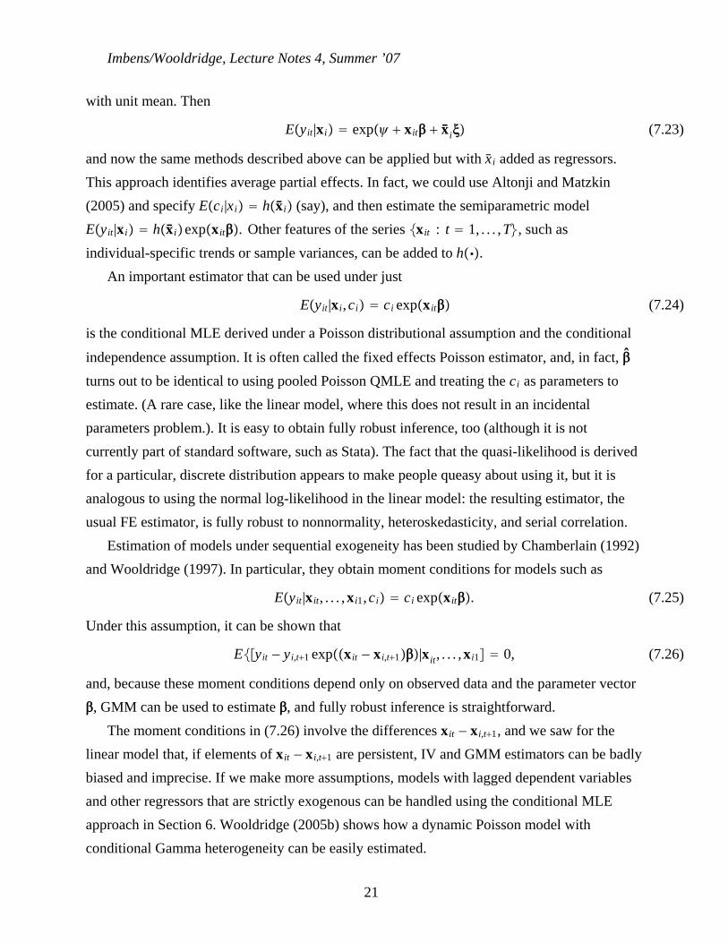
Imbens/Wooldridge, Lecture Notes 4, Summer ’07
with unit mean. Then
Eyit|xi exp xit xi (7.23)
and now the same methods described above can be applied but with xi added as regressors.This approach identifies average partial effects. In fact, we could use Altonji and Matzkin(2005) and specify Eci|xi hxi (say), and then estimate the semiparametric modelEyit|xi hxiexpxit. Other features of the series xit : t 1, . . . ,T, such asindividual-specific trends or sample variances, can be added to h.
An important estimator that can be used under just
Eyit|xi,ci ci expxit (7.24)
is the conditional MLE derived under a Poisson distributional assumption and the conditional
independence assumption. It is often called the fixed effects Poisson estimator, and, in fact, turns out to be identical to using pooled Poisson QMLE and treating the ci as parameters toestimate. (A rare case, like the linear model, where this does not result in an incidentalparameters problem.). It is easy to obtain fully robust inference, too (although it is notcurrently part of standard software, such as Stata). The fact that the quasi-likelihood is derivedfor a particular, discrete distribution appears to make people queasy about using it, but it isanalogous to using the normal log-likelihood in the linear model: the resulting estimator, theusual FE estimator, is fully robust to nonnormality, heteroskedasticity, and serial correlation.
Estimation of models under sequential exogeneity has been studied by Chamberlain (1992)and Wooldridge (1997). In particular, they obtain moment conditions for models such as
Eyit|xit, . . . ,xi1,ci ci expxit. (7.25)
Under this assumption, it can be shown that
Eyit − yi,t1 expxit − xi,t1|xit, . . . ,xi1 0, (7.26)
and, because these moment conditions depend only on observed data and the parameter vector, GMM can be used to estimate , and fully robust inference is straightforward.
The moment conditions in (7.26) involve the differences xit − xi,t1, and we saw for thelinear model that, if elements of xit − xi,t1 are persistent, IV and GMM estimators can be badlybiased and imprecise. If we make more assumptions, models with lagged dependent variablesand other regressors that are strictly exogenous can be handled using the conditional MLEapproach in Section 6. Wooldridge (2005b) shows how a dynamic Poisson model withconditional Gamma heterogeneity can be easily estimated.
21
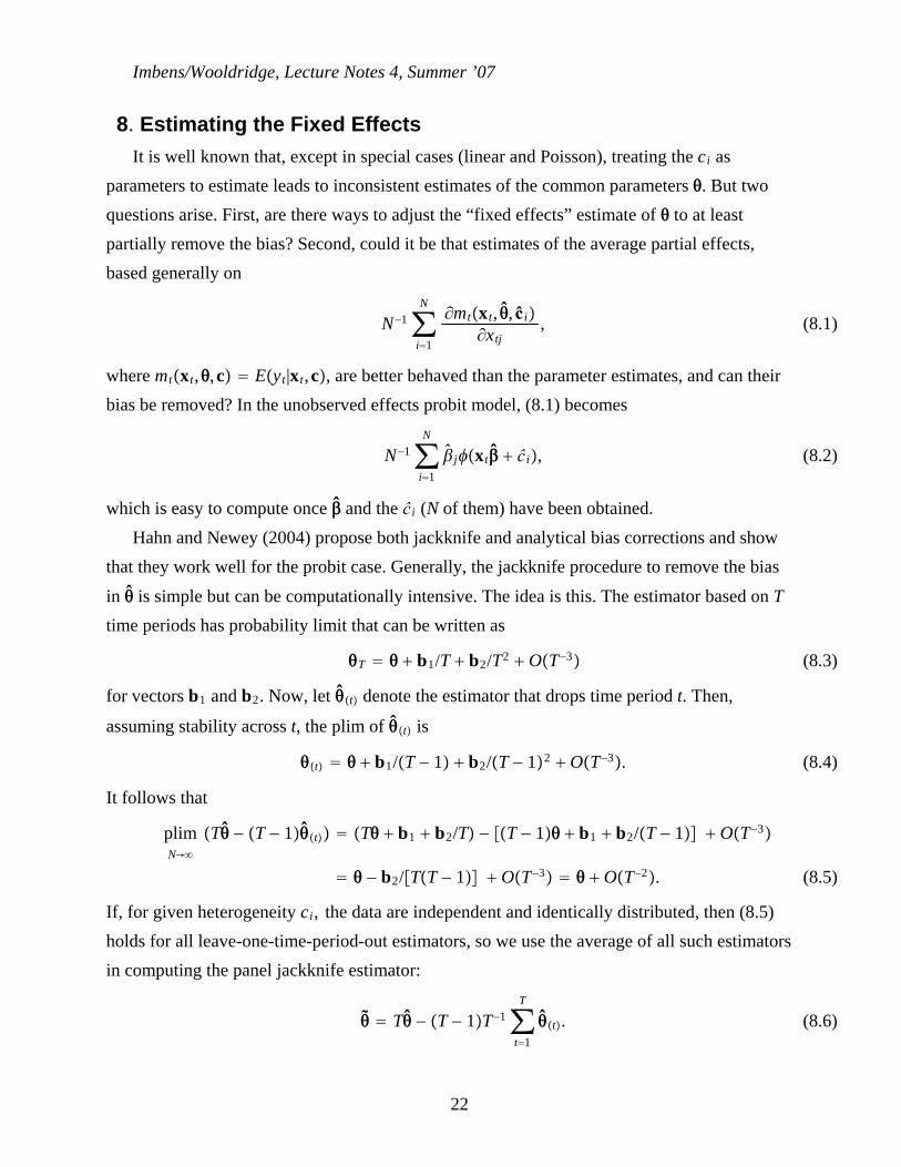
Imbens/Wooldridge, Lecture Notes 4, Summer ’07
8. Estimating the Fixed EffectsIt is well known that, except in special cases (linear and Poisson), treating the ci as
parameters to estimate leads to inconsistent estimates of the common parameters . But twoquestions arise. First, are there ways to adjust the “fixed effects” estimate of to at leastpartially remove the bias? Second, could it be that estimates of the average partial effects,based generally on
N−1∑i1
N∂mtxt, ,ĉ i
∂xtj, (8.1)
where mtxt,,c Eyt|xt,c, are better behaved than the parameter estimates, and can theirbias be removed? In the unobserved effects probit model, (8.1) becomes
N−1∑i1
N
jxt ĉ i, (8.2)
which is easy to compute once and the ĉ i (N of them) have been obtained.Hahn and Newey (2004) propose both jackknife and analytical bias corrections and show
that they work well for the probit case. Generally, the jackknife procedure to remove the biasin is simple but can be computationally intensive. The idea is this. The estimator based on Ttime periods has probability limit that can be written as
T b1/T b2/T2 OT−3 (8.3)
for vectors b1 and b2. Now, let t denote the estimator that drops time period t. Then,
assuming stability across t, the plim of t is
t b1/T − 1 b2/T − 12 OT−3. (8.4)
It follows that
N→plim T − T − 1t T b1 b2/T − T − 1 b1 b2/T − 1 OT−3
− b2/TT − 1 OT−3 OT−2. (8.5)
If, for given heterogeneity ci, the data are independent and identically distributed, then (8.5)holds for all leave-one-time-period-out estimators, so we use the average of all such estimatorsin computing the panel jackknife estimator:
T − T − 1T−1∑t1
T
t. (8.6)
22

Imbens/Wooldridge, Lecture Notes 4, Summer ’07
From the argument above, theasymptotic bias of is on the order of T−2.Unfortunately, there are some practical limitations to the jackknife procedure, as well as to
the analytical corrections derived by Hahn and Newey. First, aggregate time effects are notallowed, and they would be very difficult to include because the analysis is with T → . (Inother words, they would introduce an incidental parameters problem in the time dimension aswell as cross section dimension.) Generally, heterogeneity in the distributions across t changesthe bias terms b1 and b2 when a time period is dropped, and so the simple transformation in(8.5) does not remove the bias terms. Second, Hahn and Newey assume independence across tconditional on ci. It is a traditional assumption, but in static models it is often violated, and itmust be violated in dynamic models. Plus, as noted by Hahn and Keursteiner, applying the“leave-one-out” method to dynamic models is problematical because the b1 and b2 in (8.4)would depend on t so, again, the transformation in (8.5) will not eliminate the b1 term.
Recently, Dhaene, Jochmans, and Thuysbaert (2006) propose a modification of theHahn-Newey procedure that appears promising for dynamic models. In the simplest case, inaddition to the “fixed effects” estimator using all time periods, they obtain estimators for twosubperiods: one uses the earlier time periods, one uses later time periods, and they have someoverlap (which is small as T gets large). Unfortunately, the procedure still requires stationarityand rules out aggregate time effects.
For the probit model, Fernández-Val (2007) studies the properties of estimators andaverage partial effects and allows time series dependence in the strictly exogenous regressors.Interestingly, in the probit model with exogenous regressors under the conditionalindependence assumption, the estimates of the APEs based on the “fixed” effects estimator hasbias of order T−2 in the case that there is no heterogeneity. Unfortunately, these findings do notcarry over to models with lagged dependent variables, and the bias corrections in that case aredifficult to implement (and still do not allow for time heterogeneity).
The correlated random effects estimators restrict Dci|xi in some way, although the recentwork by Altonji and Matzkin (2005) shows how those restrictions can be made reasonable. Theapproach generally identifies the APEs, and even the local average effects, and does not ruleout aggregate time effects or arbitrary conditional serial dependence.References
(To be added.)
23
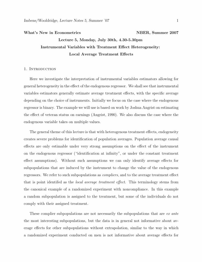
Imbens/Wooldridge, Lecture Notes 5, Summer ’07 1
What’s New in Econometrics NBER, Summer 2007
Lecture 5, Monday, July 30th, 4.30-5.30pm
Instrumental Variables with Treatment Effect Heterogeneity:
Local Average Treatment Effects
1. Introduction
Here we investigate the interpretation of instrumental variables estimators allowing for
general heterogeneity in the effect of the endogenous regressor. We shall see that instrumental
variables estimators generally estimate average treatment effects, with the specific average
depending on the choice of instruments. Initially we focus on the case where the endogenous
regressor is binary. The example we will use is based on work by Joshua Angrist on estimating
the effect of veteran status on earnings (Angrist, 1990). We also discuss the case where the
endogenous variable takes on multiple values.
The general theme of this lecture is that with heterogenous treatment effects, endogeneity
creates severe problems for identification of population averages. Population average causal
effects are only estimable under very strong assumptions on the effect of the instrument
on the endogenous regressor (“identification at infinity”, or under the constant treatment
effect assumptions). Without such assumptions we can only identify average effects for
subpopulations that are induced by the instrument to change the value of the endogenous
regressors. We refer to such subpopulations as compliers, and to the average treatment effect
that is point identifed as the local average treatment effect. This terminology stems from
the canonical example of a randomized experiment with noncompliance. In this example
a random subpopulation is assigned to the treatment, but some of the individuals do not
comply with their assigned treatment.
These complier subpopulations are not necessarily the subpopulations that are ex ante
the most interesting subpopulations, but the data is in general not informative about av-
erage effects for other subpopulations without extrapolation, similar to the way in which
a randomized experiment conducted on men is not informative about average effects for
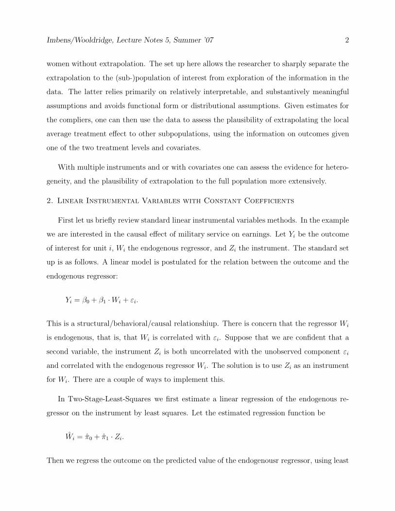
Imbens/Wooldridge, Lecture Notes 5, Summer ’07 2
women without extrapolation. The set up here allows the researcher to sharply separate the
extrapolation to the (sub-)population of interest from exploration of the information in the
data. The latter relies primarily on relatively interpretable, and substantively meaningful
assumptions and avoids functional form or distributional assumptions. Given estimates for
the compliers, one can then use the data to assess the plausibility of extrapolating the local
average treatment effect to other subpopulations, using the information on outcomes given
one of the two treatment levels and covariates.
With multiple instruments and or with covariates one can assess the evidence for hetero-
geneity, and the plausibility of extrapolation to the full population more extensively.
2. Linear Instrumental Variables with Constant Coefficients
First let us briefly review standard linear instrumental variables methods. In the example
we are interested in the causal effect of military service on earnings. Let Yi be the outcome
of interest for unit i, Wi the endogenous regressor, and Zi the instrument. The standard set
up is as follows. A linear model is postulated for the relation between the outcome and the
endogenous regressor:
Yi = β0 + β1 ·Wi + εi.
This is a structural/behavioral/causal relationshiup. There is concern that the regressor Wi
is endogenous, that is, that Wi is correlated with εi. Suppose that we are confident that a
second variable, the instrument Zi is both uncorrelated with the unobserved component εi
and correlated with the endogenous regressor Wi. The solution is to use Zi as an instrument
for Wi. There are a couple of ways to implement this.
In Two-Stage-Least-Squares we first estimate a linear regression of the endogenous re-
gressor on the instrument by least squares. Let the estimated regression function be
Wi = π0 + π1 · Zi.
Then we regress the outcome on the predicted value of the endogenousr regressor, using least
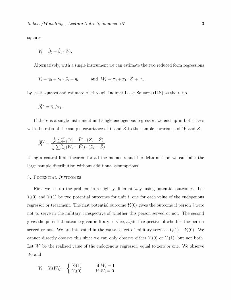
Imbens/Wooldridge, Lecture Notes 5, Summer ’07 3
squares:
Yi = β0 + β1 · Wi.
Alternatively, with a single instrument we can estimate the two reduced form regressions
Yi = γ0 + γ1 · Zi + ηi, and Wi = π0 + π1 · Zi + νi,
by least squares and estimate β1 through Indirect Least Squares (ILS) as the ratio
βIV1 = γ1/π1.
If there is a single instrument and single endogenous regressor, we end up in both cases
with the ratio of the sample covariance of Y and Z to the sample covariance of W and Z.
βIV1 =
1N
∑N
i=1(Yi − Y ) · (Zi − Z)1N
∑N
i=1(Wi − W ) · (Zi − Z).
Using a central limit theorem for all the moments and the delta method we can infer the
large sample distribution without additional assumptions.
3. Potential Outcomes
First we set up the problem in a slightly different way, using potential outcomes. Let
Yi(0) and Yi(1) be two potential outcomes for unit i, one for each value of the endogenous
regressor or treatment. The first potential outcome Yi(0) gives the outcome if person i were
not to serve in the military, irrespective of whether this person served or not. The second
gives the potential outcome given military service, again irrespective of whether the person
served or not. We are interested in the causal effect of military service, Yi(1) − Yi(0). We
cannot directly observe this since we can only observe either Yi(0) or Yi(1), but not both.
Let Wi be the realized value of the endogenous regressor, equal to zero or one. We observe
Wi and
Yi = Yi(Wi) =
Yi(1) if Wi = 1Yi(0) if Wi = 0.
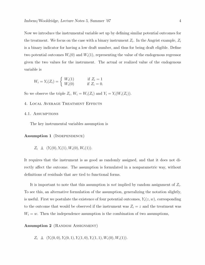
Imbens/Wooldridge, Lecture Notes 5, Summer ’07 4
Now we introduce the instrumental variable set up by defining similar potential outcomes for
the treatment. We focus on the case with a binary instrument Zi. In the Angrist example, Zi
is a binary indicator for having a low draft number, and thus for being draft eligible. Define
two potential outcomes Wi(0) and Wi(1), representing the value of the endogenous regressor
given the two values for the instrument. The actual or realized value of the endogenous
variable is
Wi = Yi(Zi) =
Wi(1) if Zi = 1Wi(0) if Zi = 0.
So we observe the triple Zi, Wi = Wi(Zi) and Yi = Yi(Wi(Zi)).
4. Local Average Treatment Effects
4.1. Assumptions
The key instrumental variables assumption is
Assumption 1 (Independence)
Zi ⊥⊥ (Yi(0), Yi(1), Wi(0), Wi(1)).
It requires that the instrument is as good as randomly assigned, and that it does not di-
rectly affect the outcome. The assumption is formulated in a nonparametric way, without
definitions of residuals that are tied to functional forms.
It is important to note that this assumption is not implied by random assignment of Zi.
To see this, an alternative formulation of the assumption, generalizing the notation slightly,
is useful. First we postulate the existence of four potential outcomes, Yi(z, w), corresponding
to the outcome that would be observed if the instrument was Zi = z and the treatment was
Wi = w. Then the independence assumption is the combination of two assumptions,
Assumption 2 (Random Assignment)
Zi ⊥⊥ (Yi(0, 0), Yi(0, 1), Yi(1, 0), Yi(1, 1), Wi(0), Wi(1)).
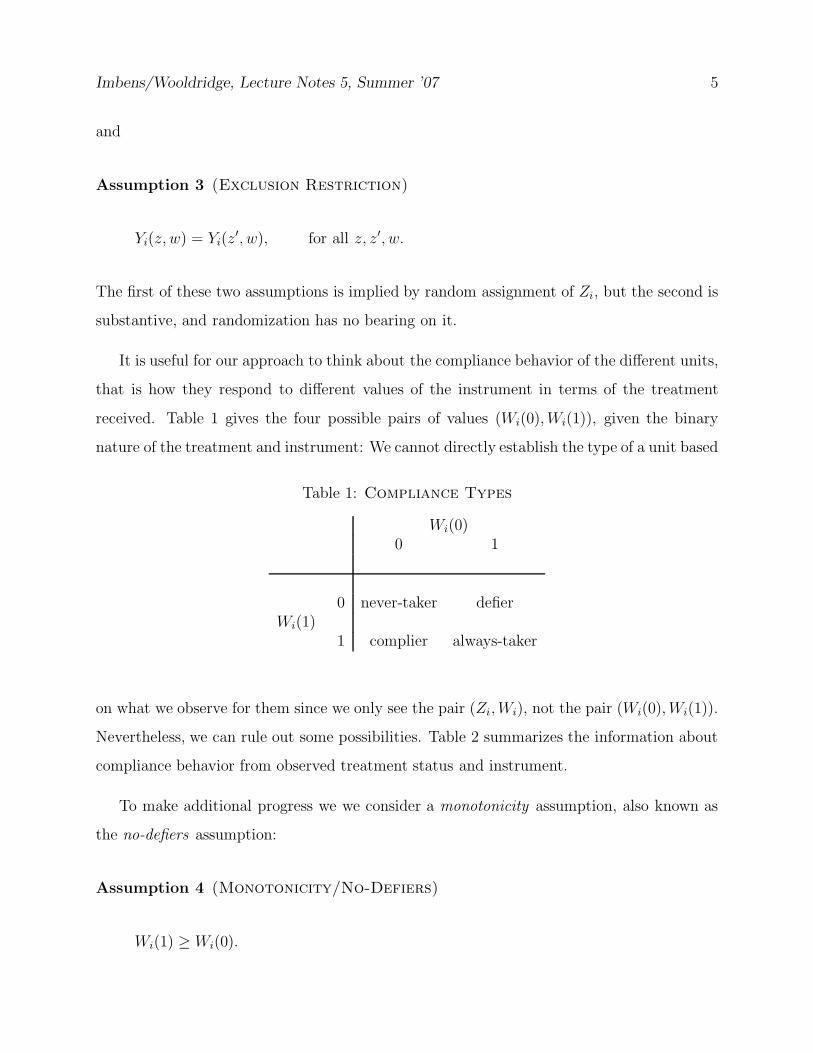
Imbens/Wooldridge, Lecture Notes 5, Summer ’07 5
and
Assumption 3 (Exclusion Restriction)
Yi(z, w) = Yi(z′, w), for all z, z′, w.
The first of these two assumptions is implied by random assignment of Zi, but the second is
substantive, and randomization has no bearing on it.
It is useful for our approach to think about the compliance behavior of the different units,
that is how they respond to different values of the instrument in terms of the treatment
received. Table 1 gives the four possible pairs of values (Wi(0), Wi(1)), given the binary
nature of the treatment and instrument: We cannot directly establish the type of a unit based
Table 1: Compliance Types
Wi(0)0 1
0 never-taker defierWi(1)
1 complier always-taker
on what we observe for them since we only see the pair (Zi, Wi), not the pair (Wi(0), Wi(1)).
Nevertheless, we can rule out some possibilities. Table 2 summarizes the information about
compliance behavior from observed treatment status and instrument.
To make additional progress we we consider a monotonicity assumption, also known as
the no-defiers assumption:
Assumption 4 (Monotonicity/No-Defiers)
Wi(1) ≥ Wi(0).
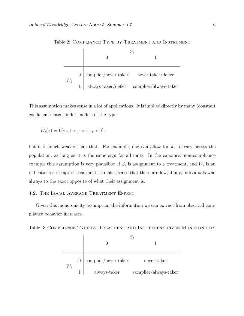
Imbens/Wooldridge, Lecture Notes 5, Summer ’07 6
Table 2: Compliance Type by Treatment and Instrument
Zi
0 1
0 complier/never-taker never-taker/defierWi
1 always-taker/defier complier/always-taker
This assumption makes sense in a lot of applications. It is implied directly by many (constant
coefficient) latent index models of the type:
Wi(z) = 1π0 + π1 · z + εi > 0,
but it is much weaker than that. For example, one can allow for π1 to vary across the
population, as long as it is the same sign for all units. In the canonical non-compliance
example this assumption is very plausible: if Zi is assignment to a treatment, and Wi is an
indicator for receipt of treatment, it makes sense that there are few, if any, individuals who
always to the exact opposite of what their assignment is.
4.2. The Local Average Treatment Effect
Given this monotonicity assumption the information we can extract from observed com-
pliance behavior increases.
Table 3: Compliance Type by Treatment and Instrument given Monotonicity
Zi
0 1
0 complier/never-taker never-takerWi
1 always-taker complier/always-taker
Imbens/Wooldridge, Lecture Notes 5, Summer ’07 7
Let πc, πn, and πa be the population proportions of compliers, never-takers and always-
takers respectively. We can estimate those from the population distribution of treatment
and instrument status:
E[Wi|Zi = 0] = πa, E[Wi|Zi = 1] = πa + πc,
which we can invert to infer the population shares of the different types:
πa = E[Wi|Zi = 0], πc = E[Wi|Zi = 1] − E[Wi|Zi = 0],
and
πn = 1 − E[Wi|Zi = 1].
Now consider average outcomes by instrument and treatment status:
E[Yi|Wi = 0, Zi = 0] =πc
πc + πn
· E[Yi(0)|complier] +πn
πc + πn
· E[Yi(0)|never− taker],
E[Yi|Wi = 0, Zi = 1] = E[Yi(0)|never− taker],
E[Yi|Wi = 1, Zi = 0] = E[Yi(1)|always − taker],
and
E[Yi|Wi = 1, Zi = 1] =πc
πc + πa
· E[Yi(1)|complier] +πa
πc + πa
· E[Yi(1)|always − taker].
From these relationships we can infer the average outcome by treatment status for compliers,
E[Yi(0)|complier], and E[Yi(1)|complier],
and thus the average effect for compliers:
E[Y (1) − Yi(0)|complier] = E[Yi(1)|complier] − E[Yi(0)|complier].
Imbens/Wooldridge, Lecture Notes 5, Summer ’07 8
We can also get there another way. Consider the least squares regression of Y on a constant
and Z. The slope coefficient in that regression estimates
E[Yi|Zi = 1] − E[Yi|Zi = 0].
Consider the first term:
E[Yi|Zi = 1] = E[Yi|Zi = 1, complier] · Pr(complier|Zi = 1)
+E[Yi|Zi = 1, never− taker] · Pr(never− taker|Zi = 1)
+E[Yi|Zi = 1, always − taker] · Pr(always − taker|Zi = 1)
= E[Yi(1)|complier] · πc
+E[Yi(0)|never− taker] · π0 + E[Yi(1)|always − taker] · πa.
Similarly
E[Yi|Zi = 0] = E[Yi|Zi = 0, complier] · Pr(complier|Zi = 0)
+E[Yi|Zi = 0, never− taker] · Pr(never− taker|Zi = 0)
+E[Yi|Zi = 0, always − taker] · Pr(always − taker|Zi = 0)
= E[Yi(0)|complier] · πc
+E[Yi(0)|never− taker] · π0 + E[Yi(1)|always − taker] · πa.
Hence the difference is
E[Yi|Zi = 1] − E[Yi|Zi = 0] = E[Yi(1) − Yi(0)|complier] · πc.
Imbens/Wooldridge, Lecture Notes 5, Summer ’07 9
The same argument can be used to show that the slope coefficient in the regression of W on
Z is
E[Wi|Zi = 1] − E[Wi|Zi = 0] = πc.
Hence the instrumental variables estimand, the ratio of these two reduced form estimands,
is equal to the local average treatment effect
βIV =E[Yi|Zi = 1] − E[Yi|Zi = 0]
E[Wi|Zi = 1] − E[Wi|Zi = 0]= E[Yi(1) − Yi(0)|complier].
The key insight is that the data are informative solely about the average effect for compli-
ers only. Put differently, the data are not informative about the average effect for nevertakers
because they are never seen receiving the treatment, and they are not informative about the
average effect for alwaystakers because they are never seen without the treatment. A similar
insight in a parametric setting is discussed in Bjorklund and Moffitt (1987).
A special case of considerable interest is that with one-side non-compliance. Suppose
that Wi(0) = 0, so that those assigned to the control group cannot receive the active treat-
ment (but those assigned to the active treatment can decline to take it). In that case only
two compliance types remain, compliers and always-takers. Monotonicity is automatically
satisfied. The average effect for compliers is now equal to the average effect for the treated,
since any one receiving the treatment is by definition a complier. This case was first studied
in Bloom (1984).
4.3 Extrapolating to the Full Population
Although we cannot consistently estimate the average effect of the treatment for always-
takers and never-takers, we do have some information about the outcomes for these subpop-
ulations given one of the two treatment arms. Specifically, we can estimate
E [Yi(0)|never− taker] , and E [Yi(1)|always − taker] .
Imbens/Wooldridge, Lecture Notes 5, Summer ’07 10
We can learn from these averages whether there is any evidence of heterogeneity in outcomes
by compliance status, by comparing the pair of average outcomes of Yi(0);
E [Yi(0)|never− taker] , and E [Yi(0)|complier] ,
and the pair of average outcomes of Yi(1):
E [Yi(1)|always − taker] , and E [Yi(1)|complier] .
If compliers, never-takers and always-takers are found to be substantially different in levels,
by evidence of substantial difference between E[Yi(0)|never− taker] and E[Yi(0)|complier],
and or/between E[Yi(1)|always − taker], and E[Yi(1)|complier], then it appears much less
plausible that the average effect for compliers is indicative of average effects for other com-
pliance types. On the other hand, if one finds that outcomes given the control treatment
for never-takers and compliers are similar, and outcomes given the treatment are similar
for compliers and always-takers, it is more plausible that average treatment effects for these
groups are also comparable.
4.4 Covariates
The local average treatment effect result implies in general that one cannot consistently
estimate average effects for subpopulations other than compliers. This still holds in cases
where we observe covariates. One can incorporate the covariates into the analysis in a number
of different ways. Traditionally the TSLS set up is used with the covariates entering in the
outcome equation linearly and additively, as
Yi = β0 + β1 ·Wi + β ′2Xi + εi,
with the covariates added to the set of instruments. Given the potential outcome set up
with general heterogeneity in the effects of the treatment, one may also wish to allow for
more heterogeneity in the correlations with the covariates. Here we describe a general way
of doing so. Unlike TSLS type approaches, this involves modelling both the dependence of
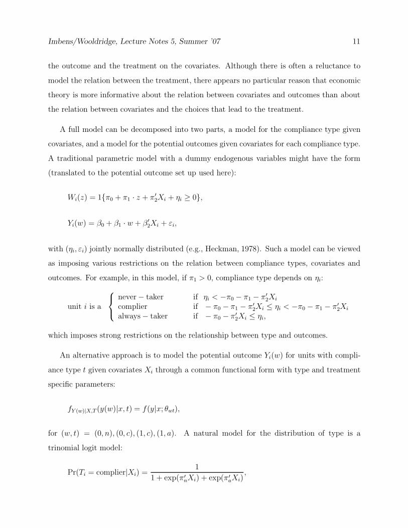
Imbens/Wooldridge, Lecture Notes 5, Summer ’07 11
the outcome and the treatment on the covariates. Although there is often a reluctance to
model the relation between the treatment, there appears no particular reason that economic
theory is more informative about the relation between covariates and outcomes than about
the relation between covariates and the choices that lead to the treatment.
A full model can be decomposed into two parts, a model for the compliance type given
covariates, and a model for the potential outcomes given covariates for each compliance type.
A traditional parametric model with a dummy endogenous variables might have the form
(translated to the potential outcome set up used here):
Wi(z) = 1π0 + π1 · z + π′2Xi + ηi ≥ 0,
Yi(w) = β0 + β1 · w + β ′2Xi + εi,
with (ηi, εi) jointly normally distributed (e.g., Heckman, 1978). Such a model can be viewed
as imposing various restrictions on the relation between compliance types, covariates and
outcomes. For example, in this model, if π1 > 0, compliance type depends on ηi:
unit i is a
never− taker if ηi < −π0 − π1 − π′2Xi
complier if − π0 − π1 − π′2Xi ≤ ηi < −π0 − π1 − π′
2Xi
always − taker if − π0 − π′2Xi ≤ ηi,
which imposes strong restrictions on the relationship between type and outcomes.
An alternative approach is to model the potential outcome Yi(w) for units with compli-
ance type t given covariates Xi through a common functional form with type and treatment
specific parameters:
fY (w)|X,T (y(w)|x, t) = f(y|x; θwt),
for (w, t) = (0, n), (0, c), (1, c), (1, a). A natural model for the distribution of type is a
trinomial logit model:
Pr(Ti = complier|Xi) =1
1 + exp(π′nXi) + exp(π′
aXi),
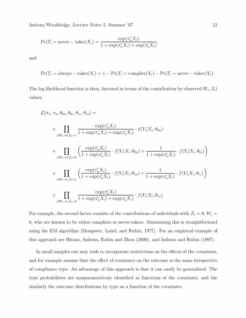
Imbens/Wooldridge, Lecture Notes 5, Summer ’07 12
Pr(Ti = never− taker|Xi) =exp(π′
nXi)
1 + exp(π′nXi) + exp(π′
aXi),
and
Pr(Ti = always − taker|Xi) = 1 − Pr(Ti = complier|Xi) − Pr(Ti = never− taker|Xi).
The log likelihood function is then, factored in terms of the contribution by observed Wi, Zi)
values:
L(πn, πa, θ0n, θ0c, θ1c, θ1a) =
×∏
i|Wi=0,Zi=1
exp(π′nXi)
1 + exp(π′nXi) + exp(π′
aXi)· f(Yi|Xi; θ0n)
×∏
i|Wi=0,Zi=0
(
exp(π′nXi)
1 + exp(π′nXi)
· f(Yi|Xi; θ0n) +1
1 + exp(π′nXi)
· f(Yi|Xi; θ0c)
)
×∏
i|Wi=1,Zi=1
(
exp(π′aXi)
1 + exp(π′aXi)
· f(Yi|Xi; θ1a) +1
1 + exp(π′aXi)
· f(Yi|Xi; θ1c)
)
×∏
i|Wi=1,Zi=0
exp(π′aXi)
1 + exp(π′nXi) + exp(π′
aXi)· f(Yi|Xi; θ1a).
For example, the second factor consists of the contributions of individuals with Zi = 0, Wi =
0, who are known to be either compliers or never-takers. Maximizing this is straightforward
using the EM algorithm (Dempster, Laird, and Rubin, 1977). For an empirical example of
this approach see Hirano, Imbens, Rubin and Zhou (2000), and Imbens and Rubin (1997).
In small samples one may wish to incorporate restrictions on the effects of the covariates,
and for example assume that the effect of covariates on the outcome is the same irrespective
of compliance type. An advantage of this approach is that it can easily be generalized. The
type probabilities are nonparametricaly identified as functions of the covariates, and the
similarly the outcome distributions by type as a function of the covariates.
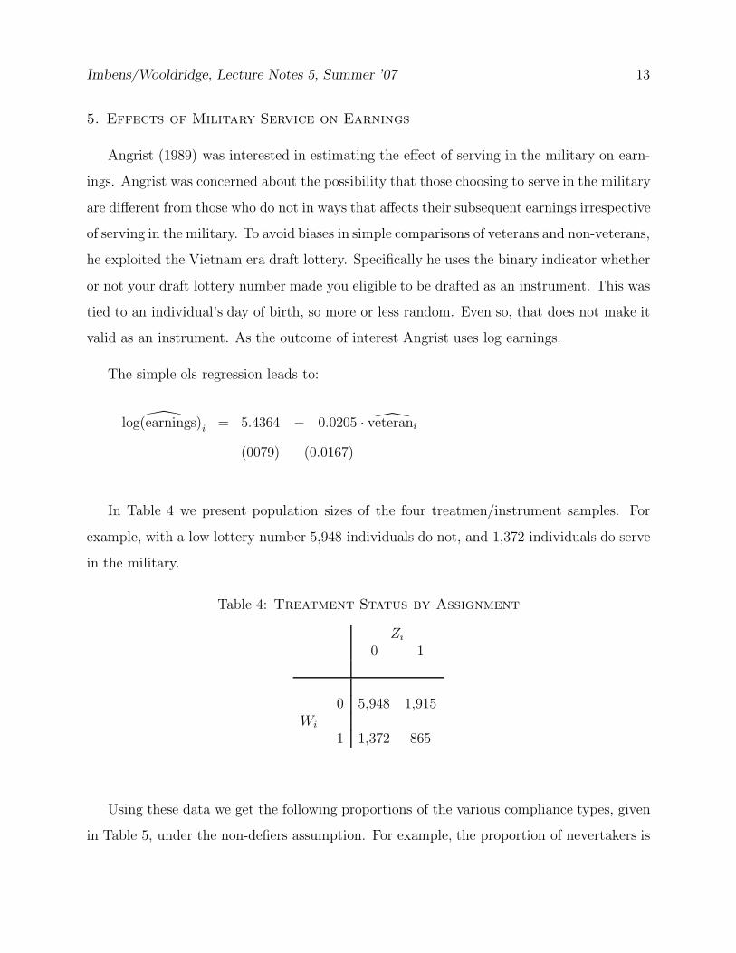
Imbens/Wooldridge, Lecture Notes 5, Summer ’07 13
5. Effects of Military Service on Earnings
Angrist (1989) was interested in estimating the effect of serving in the military on earn-
ings. Angrist was concerned about the possibility that those choosing to serve in the military
are different from those who do not in ways that affects their subsequent earnings irrespective
of serving in the military. To avoid biases in simple comparisons of veterans and non-veterans,
he exploited the Vietnam era draft lottery. Specifically he uses the binary indicator whether
or not your draft lottery number made you eligible to be drafted as an instrument. This was
tied to an individual’s day of birth, so more or less random. Even so, that does not make it
valid as an instrument. As the outcome of interest Angrist uses log earnings.
The simple ols regression leads to:
log(earnings)i = 5.4364 − 0.0205 · veterani
(0079) (0.0167)
In Table 4 we present population sizes of the four treatmen/instrument samples. For
example, with a low lottery number 5,948 individuals do not, and 1,372 individuals do serve
in the military.
Table 4: Treatment Status by Assignment
Zi
0 1
0 5,948 1,915Wi
1 1,372 865
Using these data we get the following proportions of the various compliance types, given
in Table 5, under the non-defiers assumption. For example, the proportion of nevertakers is
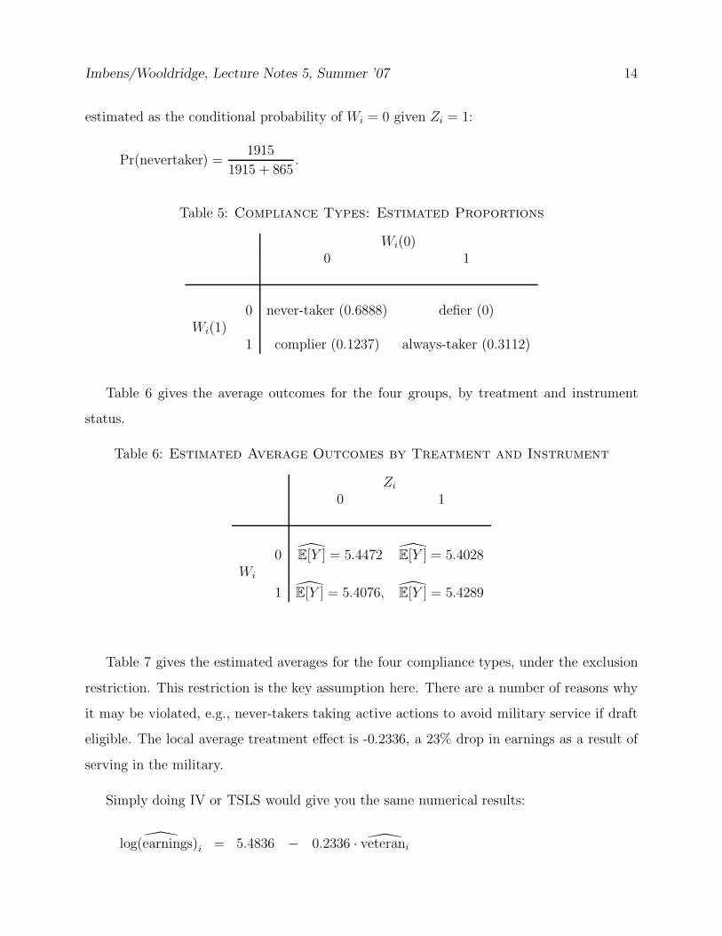
Imbens/Wooldridge, Lecture Notes 5, Summer ’07 14
estimated as the conditional probability of Wi = 0 given Zi = 1:
Pr(nevertaker) =1915
1915 + 865.
Table 5: Compliance Types: Estimated Proportions
Wi(0)0 1
0 never-taker (0.6888) defier (0)Wi(1)
1 complier (0.1237) always-taker (0.3112)
Table 6 gives the average outcomes for the four groups, by treatment and instrument
status.
Table 6: Estimated Average Outcomes by Treatment and Instrument
Zi
0 1
0 E[Y ] = 5.4472 E[Y ] = 5.4028Wi
1 E[Y ] = 5.4076, E[Y ] = 5.4289
Table 7 gives the estimated averages for the four compliance types, under the exclusion
restriction. This restriction is the key assumption here. There are a number of reasons why
it may be violated, e.g., never-takers taking active actions to avoid military service if draft
eligible. The local average treatment effect is -0.2336, a 23% drop in earnings as a result of
serving in the military.
Simply doing IV or TSLS would give you the same numerical results:
log(earnings)i = 5.4836 − 0.2336 · veterani
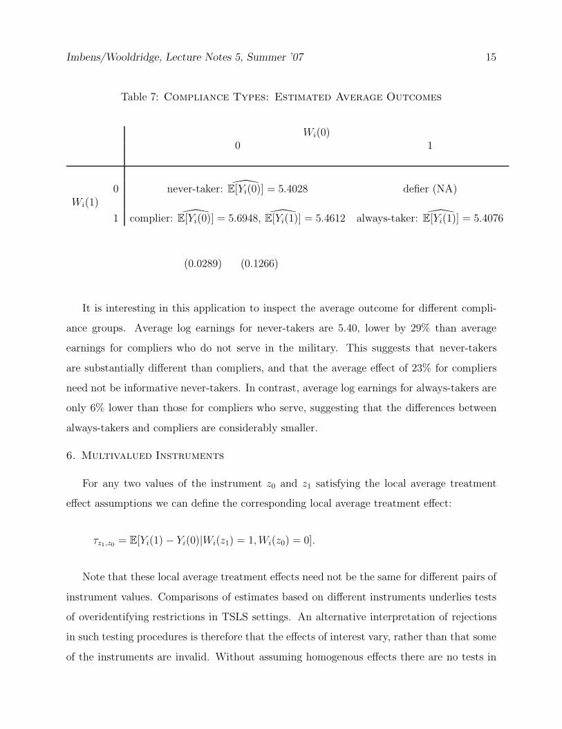
Imbens/Wooldridge, Lecture Notes 5, Summer ’07 15
Table 7: Compliance Types: Estimated Average Outcomes
Wi(0)0 1
0 never-taker: E[Yi(0)] = 5.4028 defier (NA)Wi(1)
1 complier: E[Yi(0)] = 5.6948, E[Yi(1)] = 5.4612 always-taker: E[Yi(1)] = 5.4076
(0.0289) (0.1266)
It is interesting in this application to inspect the average outcome for different compli-
ance groups. Average log earnings for never-takers are 5.40, lower by 29% than average
earnings for compliers who do not serve in the military. This suggests that never-takers
are substantially different than compliers, and that the average effect of 23% for compliers
need not be informative never-takers. In contrast, average log earnings for always-takers are
only 6% lower than those for compliers who serve, suggesting that the differences between
always-takers and compliers are considerably smaller.
6. Multivalued Instruments
For any two values of the instrument z0 and z1 satisfying the local average treatment
effect assumptions we can define the corresponding local average treatment effect:
τz1,z0 = E[Yi(1) − Yi(0)|Wi(z1) = 1, Wi(z0) = 0].
Note that these local average treatment effects need not be the same for different pairs of
instrument values. Comparisons of estimates based on different instruments underlies tests
of overidentifying restrictions in TSLS settings. An alternative interpretation of rejections
in such testing procedures is therefore that the effects of interest vary, rather than that some
of the instruments are invalid. Without assuming homogenous effects there are no tests in
Imbens/Wooldridge, Lecture Notes 5, Summer ’07 16
general for the validity of the instruments.
The presence of multi-valued, or similarly, multiple, instruments, does, however, provide
an opportunity to assess variation in treatment effects, as well as an opportunity to obtain
average effects for subpopulations closer to the one of ultimate interest. Suppose that we have
an instrument Zi with support z0, z1, . . . , zK . Suppose also that the monotonicity assumption
holds for all pairs z and z′, and suppose that the instruments are ordered in such a way that
p(zk−1) ≤ p(zk), where p(z) = E[Wi|Zi = z].
Also suppose that the instrument is relevant,
E[g(Zi) · Wi] 6= 0.
Then the instrumental variables estimator based on using g(Z) as an instrument for W
estimates a weighted average of local average treatment effects:
τg(·) =Cov(Yi, g(Zi))
Cov(Wi, g(Zi))=
K∑
k=1
λk · τzk,zk−1,
where
λk =(p(zk) − p(zk−1)) ·
∑K
l=k πl(g(zl) − E[g(Zi)]∑K
k=1 p(zk) − p(zk−1)) ·∑K
l=k πl(g(zl) − E[g(Zi)],
πk = Pr(Zi = zk).
These weights are nonnegative and sum up to one.
By choosing g(z) one can choose a different weight function, although there is obviously
a limit to what one can do. One can only estimate a weighted average of the local average
treatment effects defined for all pairs of instrument values in the support of the instrument.
Imbens/Wooldridge, Lecture Notes 5, Summer ’07 17
If the instrument is continuous, and p(z) is continuous in z, we can define the limit of the
local average treatment effects
τz = limz′↓z0,z′′↑z0
τz′,z′′ .
In this case with the monotonicity assumption hold for all pairs z and z′, we can use the
implied structure on the compliance behavior by modelling Wi(z) as a threshold crossing
process,
Wi(z) = 1h(z) + ηi ≥ 0,
with the scalar unobserved component ηi independent of the instrument Zi. This type of
latent index model is used extensively in work by Heckman (Heckman and Robb, 1985;
Heckman,1990; Heckman and Vytlacil, 2005), as well as in Vytlacil (2000). Vytlacil shows
that if the earlier three assumptions hold for all pairs z and z′, than there is a function
h(·) such that this latent index structure is consistent with the joint distribution of the
observables. The latent index structure implies that individuals can be ranked in terms of
an unobserved component ηi such that if for two individuals i and j we have ηi > ηj, than
Wi(z) ≥ Wj(z) for all z.
Given this assumption, we can define the marginal treatment effect τ (η) as
τ (η) = E [Yi(1) − Yi(0)| ηi = η] .
This marginal treatment effect relates directly to the limit of the local average treatment
effects
τ (η) = τz, with η = −h(z)).
Note that we can only define this for values of η for which there is a z such that τ = −h(z).
Normalizing the marginal distribution of η to be uniform on [0, 1] (Vytlacil, 2002), this
Imbens/Wooldridge, Lecture Notes 5, Summer ’07 18
restricts η to be in the interval [infz p(z), supz p(z)], where p(z) = Pr(Wi = 1|Zi = z).
Heckman and Vytlacil (2005) characterize various average treatment effects in terms of this
limit. For example, the average treatment effect is simply the average of the marginal
treatment effect over the marginal distribution of η:
τ =
∫
η
τ (η)dFη(η).
In practice the same limits remain on the identification of average effects. The population
average effect is only identified if the instrument moves the probability of participation from
zero to one. In fact identification of the population average treatment effect does not require
identification of τ (η) at every value of η. The latter is sufficient, but not necessary. For
example, in a randomized experiment (corresponding to a binary instrument with the treat-
ment indicator equal to the instrument) the average treatment effect is obviously identified,
but the marginal treatment effect is not for any value of η.
7. Multivalued Endogenous Variables
Now suppose that the endogenous variable W takes on values 0, 1, . . . , J . We still assume
that the instrument Z is binary. We study the interpretation of the instrumental variables
estimand
τ =Cov(Yi, Zi)
Cov(Wi, Zi)=
E[Yi|Zi = 1] − E[Yi|Zi = 0]
E[Wi|Zi = 1] − E[Wi|Zi = 0].
We make the exclusion assumption that
Yi(w) Wi(z) ⊥⊥ Zi,
and a version of the monotonicity assumption,
Wi(1) ≥ Wi(0),

Imbens/Wooldridge, Lecture Notes 5, Summer ’07 19
Then we can write the instrumental variables estimand as
τ =
J∑
j=1
λj · E[Yi(j) − Yi(j − 1)|Wi(1) ≥ j > Wi(0)],
where
λj =Pr(Wi(1) ≥ j > Wi(0)
∑J
i=1 Pr(Wi(1) ≥ i > Wi(0).
Note that we can estimate the weights λj because
Pr(Wi(1) ≥ j > Wi(0) = Pr(Wi(1) ≥ j) − Pr(Wi(0) ≥ j)
= Pr(Wi(1) ≥ j|Zi = 1) − Pr(Wi(0) ≥ j|Zi = 0)
= Pr(Wi ≥ j|Zi = 1) − Pr(Wi ≥ j|Zi = 0),
using the monotonicity assumption.
8. Instrumental Variables Estimates of the Returns to Education Using
Quarter of Birth as an Instrument
Here we use a subset of the data used by Angrist and Krueger in their 1991 study of
the returns to education. Angrist and Krueger were concerned with the endogeneity of
education, worrying that individuals with higher ability would have had higher earnings
given any level of education, as well as be more likely to have high levels of education. In
that case simple least squares estimates would over estimate the returns to education. Their
idea was that individuals born in different parts of the year are subject to slightly different
compulsory schooling laws. If you are born before a fixed cutoff date you enter school at
a younger age than if you are born after that cutoff date, and given that you are allowed
to leave school when you turn sixteen, those individuals born before the cutoff date are
required to completely more years of schooling. The instrument can therefore be thought of
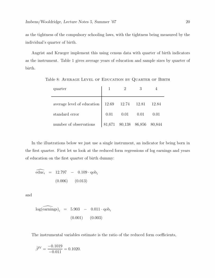
Imbens/Wooldridge, Lecture Notes 5, Summer ’07 20
as the tightness of the compulsory schooling laws, with the tightness being measured by the
individual’s quarter of birth.
Angrist and Krueger implement this using census data with quarter of birth indicators
as the instrument. Table 1 gives average years of education and sample sizes by quarter of
birth.
Table 8: Average Level of Education by Quarter of Birth
quarter 1 2 3 4
average level of education 12.69 12.74 12.81 12.84
standard error 0.01 0.01 0.01 0.01
number of observations 81,671 80,138 86,856 80,844
In the illustrations below we just use a single instrument, an indicator for being born in
the first quarter. First let us look at the reduced form regressions of log earnings and years
of education on the first quarter of birth dummy:
educi = 12.797 − 0.109 · qobi
(0.006) (0.013)
and
log(earnings)i = 5.903 − 0.011 · qobi
(0.001) (0.003)
The instrumental variables estimate is the ratio of the reduced form coefficients,
βIV =−0.1019
−0.011= 0.1020.
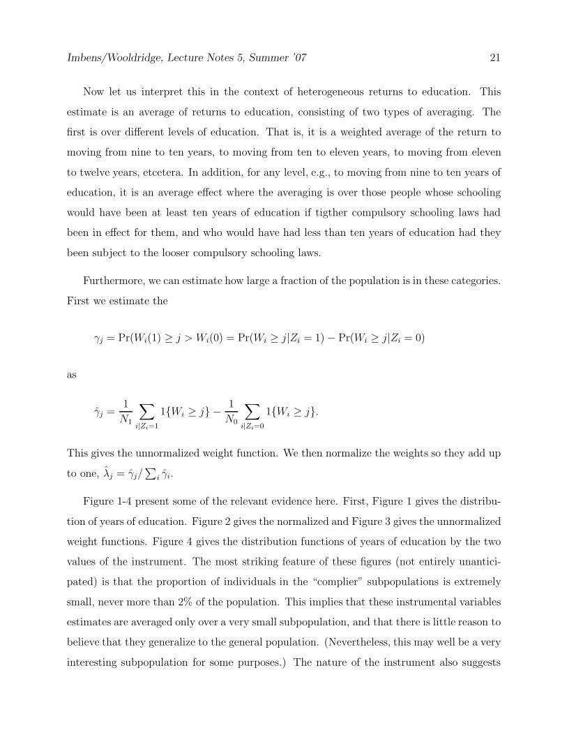
Imbens/Wooldridge, Lecture Notes 5, Summer ’07 21
Now let us interpret this in the context of heterogeneous returns to education. This
estimate is an average of returns to education, consisting of two types of averaging. The
first is over different levels of education. That is, it is a weighted average of the return to
moving from nine to ten years, to moving from ten to eleven years, to moving from eleven
to twelve years, etcetera. In addition, for any level, e.g., to moving from nine to ten years of
education, it is an average effect where the averaging is over those people whose schooling
would have been at least ten years of education if tigther compulsory schooling laws had
been in effect for them, and who would have had less than ten years of education had they
been subject to the looser compulsory schooling laws.
Furthermore, we can estimate how large a fraction of the population is in these categories.
First we estimate the
γj = Pr(Wi(1) ≥ j > Wi(0) = Pr(Wi ≥ j|Zi = 1) − Pr(Wi ≥ j|Zi = 0)
as
γj =1
N1
∑
i|Zi=1
1Wi ≥ j −1
N0
∑
i|Zi=0
1Wi ≥ j.
This gives the unnormalized weight function. We then normalize the weights so they add up
to one, λj = γj/∑
i γi.
Figure 1-4 present some of the relevant evidence here. First, Figure 1 gives the distribu-
tion of years of education. Figure 2 gives the normalized and Figure 3 gives the unnormalized
weight functions. Figure 4 gives the distribution functions of years of education by the two
values of the instrument. The most striking feature of these figures (not entirely unantici-
pated) is that the proportion of individuals in the “complier” subpopulations is extremely
small, never more than 2% of the population. This implies that these instrumental variables
estimates are averaged only over a very small subpopulation, and that there is little reason to
believe that they generalize to the general population. (Nevertheless, this may well be a very
interesting subpopulation for some purposes.) The nature of the instrument also suggests

Imbens/Wooldridge, Lecture Notes 5, Summer ’07 22
that most of the weight would be just around the number of years that would be required
under the compulsory schooling laws. The weight function is actually much flatter, putting
weight even on fourteen to fifteen years of education.
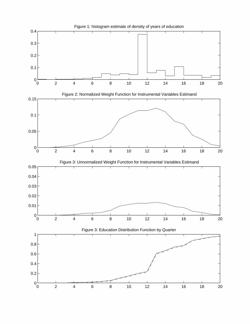
0 2 4 6 8 10 12 14 16 18 200
0.05
0.1
0.15Figure 2: Normalized Weight Function for Instrumental Variables Estimand
0 2 4 6 8 10 12 14 16 18 200
0.01
0.02
0.03
0.04
0.05Figure 3: Unnormalized Weight Function for Instrumental Variables Estimand
0 2 4 6 8 10 12 14 16 18 200
0.2
0.4
0.6
0.8
1Figure 3: Education Distribution Function by Quarter
0 2 4 6 8 10 12 14 16 18 200
0.1
0.2
0.3
0.4Figure 1: histogram estimate of density of years of education
Imbens/Wooldridge, Lecture Notes 5, Summer ’07 23
References
Angrist, J. D., and G. W. Imbens, (1995), ”Two–Stage Least Squares Estimation
of Average Causal Effects in Models with Variable Treatment Intensity,” Journal of the
American Statistical Association, Vol 90, No. 430, 431-442.
Angrist, J.D., G.W. Imbens and D.B. Rubin (1996), “Identification of Causal
Effects Using Instrumental Variables,” (with discussion) Journal of the American Statistical
Association, 91, 444-472.
Angrist, J., (1990), ”Lifetime Earnings and the Vietnam Era Draft Lottery: Evidence
from Social Security Administrative Records,” American Economic Review, 80, 313-335.
Angrist, J. and A. Krueger, (1992), ”The Effect of Age at School Entry on Ed-
ucational Attainment: An Application of Instrumental Variables with Moments from Two
Samples,” Journal of the American Statistical Association 87, June.
Bjorklund, A. and R. Moffitt, (1987), ”The Estimation of Wage Gains and Welfare
Gains in Self–Selection Models”, Review of Economics and Statistics, Vol. LXIX, 42–49.
Bloom, H., (1984), “Accounting for No–shows in Experimental Evaluation Designs,”Evaluation
Review, 8(2) 225–246.
Dempster, A., N. Laird, and D. Rubin (1977), “Maximum Likelihood Estimation
from Incomplete Data Using the EM Algorithm (with discussion),” Journal of the Royal
Statistical Society, Series B, 39, 1-38.
Heckman, J. J. (1990), ”Varieties of Selection Bias,” American Economic Review 80,
313-318.
Heckman, J., and R. Robb, (1985), “Alternative Methods for Evaluating the Impact
of Interventions,”in Heckman and Singer (eds.), Longitudinal Analysis of Labor Market Data,
Cambridge, Cambridge University Press.
Heckman, J., and E. Vytlacil, (2005), “Structural Equations, Treatment Effects,
Imbens/Wooldridge, Lecture Notes 5, Summer ’07 24
and Econometric Policy Evaluation,” Econometrica, Vol. 73(3), 669-738.
Hirano, K., G. Imbens, D. Rubin, and X. Zhou (2000), “Identification and Esti-
mation of Local Average Treatment Effects,” Biostatistics, Vol. 1(1), 69-88.
Imbens, G., and J. Angrist (1994), “Identification and Estimation of Local Average
Treatment Effects,” Econometrica, Vol. 61, No. 2, 467-476.
Imbens, G. W., and D. B. Rubin, (1997), “Bayesian Inference for Causal Effects
in Randomized Experiments with Noncompliance,”Annals of Statistics, Vol. 25, No. 1,
305–327.
Vytlacil, E., (2002), “Independence, Monotonicity, and Latent Index Models: Am
Equivalence Result,” Econometrica, Vol. 70(1), 331-341.
Imbens/Wooldridge, Lecture Notes 6, Summer ’07
What’s New in Econometrics? NBER, Summer 2007Lecture 6, Tuesday, July 31st, 9.00-10.30 am
Control Function and Related MethodsThese notes review the control function approach to handling endogeneity in models linear
in parameters, and draws comparisons with standard methods such as 2SLS. Certain nonlinearmodels with endogenous explanatory variables are most easily estimated using the CF method,and the recent focus on average marginal effects suggests some simple, flexible strategies.Recent advances in semiparametric and nonparametric control function method are covered,and an example for how one can apply CF methods to nonlinear panel data models is provided.1. Linear-in-Parameters Models: IV versus Control Functions
Most models that are linear in parameters are estimated using standard IV methods – eithertwo stage least squares (2SLS) or generalized method of moments (GMM). An alternative, thecontrol function (CF) approach, relies on the same kinds of identification conditions. In thestandard case where a endogenous explanatory variables appear linearly, the CF approachleads to the usual 2SLS estimator. But there are differences for models nonlinear inendogenous variables even if they are linear in parameters. And, for models nonlinear inparameters, the CF approach offers some distinct advantages.
Let y1 denote the response variable, y2 the endogenous explanatory variable (a scalar forsimplicity), and z the 1 L vector of exogenous variables (which includes unity as its firstelement). Consider the model
y1 z11 1y2 u1 (1.1)
where z1 is a 1 L1 strict subvector of z that also includes a constant. The sense in which z isexogenous is given by the L orthogonality (zero covariance) conditions
Ez′u1 0. (1.2)
Of course, this is the same exogeneity condition we use for consistency of the 2SLS estimator,and we can consistently estimate 1 and 1 by 2SLS under (1.2) and the rank condition,Assumption 2SLS.2.
Just as with 2SLS, the reduced form of y2 – that is, the linear projection of y2 onto theexogenous variables – plays a critical role. Write the reduced form with an error term as
y2 z2 v2
Ez′v2 0 (1.3) (1.4)
where 2 is L 1. Endogeneity of y2 arises if and only if u1 is correlated with v2. Write the
1
Imbens/Wooldridge, Lecture Notes 6, Summer ’07
linear projection of u1 on v2, in error form, as
u1 1v2 e1, (1.5)
where 1 Ev2u1/Ev22 is the population regression coefficient. By definition, Ev2e1 0,
and Ez′e1 0 because u1 and v2 are both uncorrelated with z.Plugging (1.5) into equation (1.1) gives
y1 z11 1y2 1v2 e1, (1.6)
where we now view v2 as an explanatory variable in the equation. As just noted, e1, isuncorrelated with v2 and z. Plus, y2 is a linear function of z and v2, and so e1 is alsouncorrelated with y2.
Because e1 is uncorrelated with z1, y2, and v2, (1.6) suggests a simple procedure forconsistently estimating 1 and 1 (as well as 1): run the OLS regression of y1 on z1,y2, and v2
using a random sample. (Remember, OLS consistently estimates the parameters in anyequation where the error term is uncorrelated with the right hand side variables.) The onlyproblem with this suggestion is that we do not observe v2; it is the error in the reduced formequation for y2. Nevertheless, we can write v2 y2 − z2 and, because we collect data on y2
and z, we can consistently estimate 2 by OLS. Therefore, we can replace v2 with v2, the OLSresiduals from the first-stage regression of y2 on z. Simple substitution gives
y1 z11 1y2 1v2 error, (1.7)
where, for each i, errori ei1 1zi2 − 2, which depends on the sampling error in 2
unless 1 0. Standard results on two-step estimation imply the OLS estimators from (1.7)will be consistent for 1,1, and 1.
The OLS estimates from (1.7) are control function estimates. The inclusion of the residualsv2 “controls” for the endogeneity of y2 in the original equation (although it does so withsampling error because 2 ≠ 2).
It is a simple exercise in the algebra of least squares to show that the OLS estimates of 1
and 1 from (1.7) are identical to the 2SLS estimates starting from (1.1) and using z as thevector of instruments. (Standard errors from (1.7) must adjust for the generated regressor.)
It is trivial to use (1.7) to test H0 : 1 0, as the usual t statistic is asymptotically validunder homoskedasticity Varu1|z,y2 1
2 under H0; or use the heteroskedasticity-robustversion (which does not account for the first-stage estimation of 2).
Now extend the model:
2
Imbens/Wooldridge, Lecture Notes 6, Summer ’07
y1 z11 1y2 1y22 u1
Eu1|z 0. (1.8) (1.9)
For simplicity, assume that we have a scalar, z2, that is not also in z1. Then, under (1.9) –which is stronger than (1.2), and is essentially needed to identify nonlinear models – we canuse, say, z2
2 (if z2 is not binary) as an instrument for y22 because any function of z2 is
uncorrelated with u1. In other words, we can apply the standard IV estimator with explanatoryvariables z1,y2,y2
2 and instruments z1, z2, z22; note that we have two endogenous
explanatory variables, y2 and y22.
What would the CF approach entail in this case? To implement the CF approach in (1.8),we obtain the conditional expectation Ey1|z,y2 – a linear projection argument no longerworks because of the nonlinearity – and that requires an assumption about Eu1|z,y2. Astandard assumption is
Eu1|z,y2 Eu1|z,v2 Eu1|v2 1v2, (1.10)
where the first equality follows because y2 and v2 are one-to-one functions of each other(given z) and the second would hold if u1,v2 is independent of z – a nontrivial restriction onthe reduced form error in (1.3), not to mention the structural error u1.. The final assumption islinearity of the conditional expectation Eu1|v2, which is more restrictive than simply defininga linear projection. Under (1.10),
Ey1|z,y2 z11 1y2 1y22 1y2 − z2
z11 1y2 1y22 1v2.
(1.11)
Implementing the CF approach means running the OLS regression y1 on z1,y2,y22, v2,where v2
still represents the reduced form residuals. The CF estimates are not the same as the 2SLSestimates using any choice of instruments for y2,y2
2.The CF approach, while likely more efficient than a direct IV approach, is less robust. For
example, it is easily seen that (1.9) and (1.10) imply that Ey2|z z2. A linear conditional
expectation for y2 is a substantive restriction on the conditional distribution of y2. Therefore,the CF estimator will be inconsistent in cases where the 2SLS estimator will be consistent. Onthe other hand, because the CF estimator solves the endogeneity of y2 and y2
2 by adding thescalar v2 to the regression, it will generally be more precise – perhaps much more precise –than the IV estimator. (I do not know of a systematic analysis comparing the two approaches inmodels such as (1.8).)
3
Imbens/Wooldridge, Lecture Notes 6, Summer ’07
Standard CF approaches impose extra assumptions even in the simple model (1.1) if weallow y2 to have discreteness in its distribution. For example, suppose y2 is a binary response.Then the CF approach involves estimating
Ey1|z,y2 z11 1y2 Eu1|z,y2,
and so we must be able to estimate Eu1|z,y2. If y2 1z2 e2 ≥ 0, u1,e2 is independentof z, Eu1|e2 1e2, and e2 ~Normal0,1, then
Eu1|z,y2 EEu1|z,e2|z,y2 1Ev2|z,y2
1y2z2 − 1 − y2−z2,
where / is the inverse Mills ratio (IMR). A simple two-step estimator is to
obtain the probit estimator 2 and then to add the “generalized residual,”
gri2 ≡ yi2zi2 − 1 − yi2−zi2 as a regressor:
yi1 on zi1, yi2, gri2, i 1, . . . ,N.
Consistency of the CF estimators hinges on the model for Dy2|z being correctly specified,along with linearity in Eu1|v2 (and some sort of independence with z). Of course, if we justapply 2SLS directly to (1.1), it makes no distinction among discrete, continuous, or somemixture for y2. 2SLS is consistent if Ly2|z z2 actually depends on z2 and (1.2) holds. So,while estimating (1.1) using CF methods when y2 is binary is somewhat popular (Stata’s“treatreg” even has the option of full MLE, where u1,e2 is bivariate normal), one shouldremember that it is less robust than standard IV approaches.
How might one use the binary nature of y2 in IV estimation? Assume Eu1|z 0 and,
nominally, assume a probit model for Dy2|z. Obtain the fitted probabilities, zi2, from thefirst stage probit, and then use these as IVs for yi2. This method is fully robust tomisspecification of the probit model; the standard errors need not be adjusted for the first-stageprobit (asymptotically); and it is the efficient IV estimator if Py2 1|z z2 andVaru1|z 1
2. But it is probably less efficient than the CF estimator if the additional
assumptions needed for CF consistency hold. (Note: Using zi2 as an IV for yi2 is not the
same as using zi2 as a regressor in place of yi2.)To summarize: except in the case where y2 appears linearly and a linear reduced form is
estimated for y2, the CF approach imposes extra assumptions not imposed by IV approaches.However, in more complicated models, it is hard to beat the CF approach.2. Correlated Random Coefficient Models
4
Imbens/Wooldridge, Lecture Notes 6, Summer ’07
Control function methods can be used for random coefficient models – that is, modelswhere unobserved heterogeneity interacts with endogenous explanatory variables. However, insome cases, standard IV methods are more robust. To illustrate, we modify equation (1.1) as
y1 1 z11 a1y2 u1, (2.1)
where z1 is 1 L1, y2 is the endogenous explanatory variable, and a1, the “coefficient” on y2 –an unobserved random variable. [It is now convenient to set apart the intercept.] We couldreplace 1 with a random vector, say d1, and this would not affect our analysis of the IVestimator (but would slightly alter the control function estimator). Following Heckman andVytlacil (1998), we refer to (2.1) as a correlated random coefficient (CRC) model.
It is convenient to write a1 1 v1 where 1 Ea1 is the object of interest. We canrewrite the equation as
y1 1 z11 1y2 v1y2 u1 ≡ 1 z11 1y2 e1, (2.2)
where e1 v1y2 u1. Equation (2.2) shows explicitly a constant coefficient on y2 (which wehope to estimate) but also an interaction between the observed heterogeneity, v1, and y2.Remember, (2.2) is a population model. For a random draw, we would writeyi1 1 zi11 1yi2 vi1yi2 ui1, which makes it clear that 1 and 1 are parameters toestimate and vi1 is specific to observation i.
As discussed in Wooldridge (1997, 2003), the potential problem with applying instrumentalvariables (2SLS) to (2.2) is that the error term v1y2 u1 is not necessarily uncorrelated withthe instruments z, even if we make the assumptions
Eu1|z Ev1|z 0, (2.3)
which we maintain from here on. Generally, the term v1y2 can cause problems for IVestimation, but it is important to be clear about the nature of the problem. If we are allowing y2
to be correlated with u1 then we also want to allow y2 and v1 to be correlated. In other words,Ev1y2 Covv1,y2 ≡ 1 ≠ 0. But a nonzero unconditional covariance is not a problemwith applying IV to (2.2): it simply implies that the composite error term, e1, has(unconditional) mean 1 rather than a zero. As we know, a nonzero mean for e1 means that theorginal intercept, 1, would be inconsistenly estimated, but this is rarely a concern.
Therefore, we can allow Covv1,y2, the unconditional covariance, to be unrestricted. Butthe usual IV estimator is generally inconsistent if Ev1y2|z depends on z. (There are still cases,which we will cover in Part IV, where the IV estimator is consistent.). Note that, because
5
Imbens/Wooldridge, Lecture Notes 6, Summer ’07
Ev1|z 0, Ev1y2|z Covv1,y2|z. Therefore, as shown in Wooldridge (2003), asufficient condition for the IV estimator applied to (2.2) to be consistent for 1 and 1 is
Covv1,y2|z Covv1,y2. (2.4)
The 2SLS intercept estimator is consistent for 1 1. Condition (2.4) means that theconditional covariance between v1 and y2 is not a function of z, but the unconditionalcovariance is unrestricted.
Because v1 is unobserved, we cannot generally verify (2.4). But it is easy to find situationswhere it holds. For example, if we write
y2 m2z v2 (2.5)
and assume v1,v2 is independent of z (with zero mean), then (2.4) is easily seen to holdbecause Covv1,y2|z Covv1,v2|z, and the latter cannot be a function of z underindependence. Of course, assuming v2 in (2.5) is independent of z is a strong assumption evenif we do not need to specify the mean function, m2z. It is much stronger than just writingdown a linear projection of y2 on z (which is no real assumption at all). As we will see invarious models in Part IV, the representation (2.5) with v2 independent of z is not suitable fordiscrete y2, and generally (2.4) is not a good assumption when y2 has discrete characteristics.Further, as discussed in Card (2001), (2.4) can be violated even if y2 is (roughly) continuous.Wooldridge (2005a) makes some headway in relaxing (2.44) by allowing for parametricheteroskedasticity in u1 and v2.
A useful extension of (1.1) is to allow observed exogenous variables to interact with y2.The most convenient formulation is
y1 1 z11 1y2 z1 − 1y21 v1y2 u1 (2.6)
where 1 ≡ Ez1 is the 1 L1 vector of population means of the exogenous variables and 1
is an L1 1 parameter vector. As we saw in Chapter 4, subtracting the mean from z1 beforeforming the interaction with y2 ensures that 1 is the average partial effect.
Estimation of (2.6) is simple if we maintain (2.4) [along with (2.3) and the appropriate rankcondition]. Typically, we would replace the unknown 1 with the sample averages, z1, and
then estimate
yi1 1 zi11 1yi2 zi1 − z1yi21 errori (2.7)
by instrumental variables, ignoring the estimation error in the population mean. The only issue
6
Imbens/Wooldridge, Lecture Notes 6, Summer ’07
is choice of instruments, which is complicated by the interaction term. One possibility is to useinteractions between zi1 and all elements of zi (including zi1). This results in manyoveridentifying restrictions, even if we just have one instrument zi2 for yi2. Alternatively, wecould obtain fitted values from a first stage linear regression yi2 on zi, ŷ i2 zi2, and then useIVs 1,zi, zi1 − z1ŷ i2, which results in as many overidentifying restrictions as for the modelwithout the interaction. Importantly, the use of zi1 − z1ŷ i2 as IVs for zi1 − z1yi2 isasymptotically the same as using instruments zi1 − 1 zi2, where Ly2|z z2 is the
linear projection. In other words, consistency of this IV procedure does not in any way restrictthe nature of the distribution of y2 given z. Plus, although we have generated instruments, theassumptions sufficient for ignoring estimation of the instruments hold, and so inference isstandard (perhaps made robust to heteroskedasticity, as usual).
We can just identify the parameters in (2.6) by using a further restricted set of instruments,1,zi1,ŷ i2, zi1 − z1ŷ i2. If so, it is important to use these as instruments and not as regressors.If we add the assumption. The latter procedure essentially requires a new assumption:
Ey2|z z2 (2.8)
(where z includes a constant). Under (2.3), (2.4), and (2.8), it is easy to show
Ey1|z 1 1 z11 1z2 z1 − 1 z21, (2.9)
which is the basis for the Heckman and Vytlacil (1998) plug-in estimator. The usual IVapproach simply relaxes (2.8) and does not require adjustments to the standard errors (becauseit uses generated instruments, not generated regressors).
We can also use a control function approach if we assume
Eu1|z,v2 1v2,Ev1|z,v2 1v2. (2.10)
Then
Ey1|z,y2 1 z11 1y2 1v2y2 1v2, (2.11)
and this equation is estimable once we estimate 2. Garen’s (1984) control function procedureis to first regress y2 on z and obtain the reduced form residuals, v2, and then to run the OLSregression y1 on 1,z1,y2, v2y2, v2. Under the maintained assumptions, Garen’s methodconsistently estimates 1 and 1. Because the second step uses generated regressors, thestandard errors should be adjusted for the estimation of 2 in the first stage. Nevertheless, atest that y2 is exogenous is easily obtained from the usual F test of H0 : 1 0,1 0 (or aheteroskedasticity-robust version). Under the null, no adjustment is needed for the generated
7
Imbens/Wooldridge, Lecture Notes 6, Summer ’07
standard errors.Garen’s assumptions are more restrictive than those needed for the standard IV estimator to
be consistent. For one, it would be a fluke if (2.10) held without the conditional covarianceCovv1,y2|z being independent of z. Plus, like HV (1998), Garen relies on a linear model forEy2|z. Further, Garen adds the assumptions that Eu1|v2 and Ev1|v2 are linear functions,something not needed by the IV approach.
Of course, one can make Garen’s approach less parametric by replacing the linear functionsin (2.10) with unknown functions. But independence of u1,v1,v2 and z – or something veryclose to independence – is needed. And this assumption is not needed for the usual IVestimator,
If the assumptions needed for Garen’s CF estimator to be consistent hold, it is likely moreefficient than the IV estimator, although a comparison of the correct asymptotic variances iscomplicated. Again, there is a tradeoff between efficiency and robustness.
In the case of binary y2, we have what is often called the “switching regression” model.Now, the right hand side of equation (2.11) represents Ey1|z,v2 where y2 1z2 v2 ≥ 0.If we assume (2.10) and that v2|z is Normal0,1, then
Ey1|z,y2 1 z11 1y2 1h2y2,z2 1h2y2,z2y2,
where
h2y2,z2 y2z2 − 1 − y2−z2
is the generalized residual function. The two-step estimation method is the one due toHeckman (1976).
There are two ways to embellish the model. The first is common: interact z1 − 1 with y2
to allow different slopes for the “treated” and non-treated groups (keeping 1 as the averagetreatment effect). This is common, and then the CF regression
yi1 on 1, zi11 1yi2 zi1 − z1yi2, h2yi2,zi2, h2yi2,zi2yi2
is identical to running two separate regressions, including the IMRs for y2 0 and y2 1. Theestimate of 1 is then the difference in the two intercepts.
An extension that is not so common – in fact, it seems not to appear in the literature –comes from allowing z1 to also interact with heterogeneity, as in
y1 z1d1 a1y2 y2z1 − 1g1 u1.
Now all coefficients are heterogeneous. If we assume that Ea1|v2, Ed1|v2, and Eg1|v2 are
8
Imbens/Wooldridge, Lecture Notes 6, Summer ’07
linear in v2, then
Ey1|z,y2 z11 1y2 y2z1 − 11 1Ev2|z,y2 1Ev2|z,y2y2
z1Ev2|z,y21 y2z1 − 1Ev2|z,y21
z11 1y2 1h2y2,z2 1h2y2,z2y2
h2y2,z2z11 h2y2,z2y2z1 − 11
and the second-step estimation after the first stage probit is a regression
yi1 on 1, zi11 1yi2 zi1 − z1yi2, h2yi2,zi2, h2yi2,zi2yi2,h2yi2,zi2zi1, h2yi2,zi2yi2zi1 − z1.
across all observations i. It is easy use bootstrapping to obtain valid standard errors because thefirst-stage estimation is just a probit and the second stage is just linear regression.
If not for the term v1y2, we could, in a much more robust manner, use an IV procedure(where the standard errors are easier to obtain, too). The IVs would be1,zi1, i2, zi1 − z1 i2, and the same procedure consistently estimates the average effectswhether or not there are random coefficients on zi1.
Interesting, the addition of the terms h2yi2,zi2zi1 and h2yi2,zi2yi2zi1 − z1 hassimilarities with methods that allow Ev1|v2 and so on to be more flexible. For example, asshown in Heckman and MaCurdy (1986), if Eu1|v2 1v2 1v2
2 − 1, then the extra term
for y2 1 is −zi2zi2 and there is a similar expression for yi2 0.Newey (1988), in the standard switching regression framework, proposed a flexible
two-step procedure that estimates 2 semiparametrically in the first stage – see Powell (1994)
for a survey of such methods – and then uses series in zi2 in place of the usual IMR terms. Heobtains valid standard errors and, in most cases, bootstrapping is valid, too.3. Some Common Nonlinear Models and Limitations of the CFApproach
Like standard IV methods, control function approaches are more difficult to apply tononlinear models, even relatively simple ones. Methods are available when the endogenousexplanatory variables are continuous, but few if any results apply to cases with discrete y2.
3.1. Binary and Fractional Responses
The probit model provides a good illustration of the general approach. With a singleendogenous explanatory variable, the simplest specification is
y1 1z11 1y2 u1 ≥ 0, (3.1)
9
Imbens/Wooldridge, Lecture Notes 6, Summer ’07
where u1|z ~Normal0,1. But the analysis goes through if we replace z1,y2 with any knownfunction g1z1,y2, provided we have sufficient identifying assumptions. An example isy1 z11 y2z11 1y2
2 u1 0. The nonlinearity in y2 is not itself a problem (unless weinappropriately try to mimic 2SLS – more on this later).
The Blundell-Smith (1986) and Rivers-Vuong (1988) approach is to make ahomoskedastic-normal assumption on the reduced form for y2,
y2 z2 v2, v2|z ~Normal0,22. (3.2)
A key point is that the RV approach essentially requires
u1,v2 independent of z; (3.3)
as we will see in the next section, semiparametric and nonparametric CF methods also rely on(3.3), or at least something close to it..
If we assume
u1,v2 ~Bivariate Normal (3.4)
with 1 Corru1,v2, then we can proceed with MLE based on fy1,y2|z. A simplertwo-step approach, which is convenient for testing H0 : 1 0 (y2 is exogenous) is alsoavailable, and works if we replace the normality assumption in (3.2), the independenceassumption in (3.3), and joint normality in (3.4) with
Du1|v2,z Normal1v2, 1 − 12, (3.5)
where 1 1/2 is the regression coefficient. That we can relax the assumptions to somedegree using a two-step CF approach has implications for less parametric approaches.Certainly we can relax the homoskedasticity and linear expectation in (3.3) without muchadditional work, as discussed in Wooldridge (2005a).
Under the weaker assumption (3.5) we can write
Py1 1|z,y2 z11 1y2 1v2 (3.6)
where each coefficient is multiplied by 1 − 12−1/2.
The RV two-step approach is(i) OLS of y2 on z, to obtain the residuals, v2.(ii) Probit of y1 on z1,y2, v2 to estimate the scaled coefficients.
The original coefficients, which appear in the partial effects, are easily obtained from theset of two-step estimates:
10
Imbens/Wooldridge, Lecture Notes 6, Summer ’07
1 1/1 12 2
21/2, (3.7)
where 1 is the coeffcient on v2 and 22 is the usual error variance estimator from the first step
OLS, and 1 includes 1 and 1. Standard errors can be obtained from the delta method of
bootstrapping. Of course, they are computed directly from MLE. Partial effects are based on
x11 where x1 z1,y2. Hopefully it is clear that nothing changes if x1 g1z1,y2
expect how one computes the partial effects.A simple t test on v2 is valid to test H0 : 1 0.A different way to obtain partial effects is to use the average structural function approach,
which leads to Ev2x11. Notice this holds under (3.5) without joint normality. A
consistent, N -asymptotically normal estimator is
ASFz1,y2 N−1∑i1
N
x11 1vi2, (3.8)
that is, we average out the reduced form residuals, vi2. This formulation is useful for morecomplicated models.
Given that the probit structural model is essentially arbitrary, one might be so bold as tospecify models for Py1 1|z1,y2,v2 directly. For example, we can add polynomials in v2 oreven interact v2 with elements of x1 side a probit or logit function. We return to this in the nextsection.
The two-step CF approach easily extends to fractional responses. Now, we start with anomitted variables formulation in the conditional mean:
Ey1|z,y2,q1 Ey1|z1,y2,q1 x11 q1, (3.9)
where x1 is a function of z1,y2 and q1 contains unobservables. As usual, we need someexclusion restrictions, embodied by omitting z2 from x1. The specification in equation (3.9)allows for responses at the corners, zero and one, and y1 may take on any values in between.Under the assumption that
Dq1|v2,z ~ Normal1v2,12 (3.10)
Given (3.9) and (3.10), it can be shown, using the mixing property of the normal distribution,that
Ey1|z,y2,v2 x11 1v2, (3.11)
11
Imbens/Wooldridge, Lecture Notes 6, Summer ’07
where the index “” denotes coefficients multiplied by 1 12−1/2. Because the Bernoulli log
likelihood is in the linear exponential family, maximizing it consistently estimates theparameters of a correctly specified mean; naturally, the same is true for two-step estimation.That is, the same two-step method can be used in the binary and fractional cases. Of course,the variance associated with the Bernoulli distribution is generally incorrect. In addition tocorrecting for the first-stage estimates, a robust sandwich estimator should be computed toaccount for the fact that Dy1|z,y2 is not Bernoulli. The best way to compute partial effects isto use (3.8), with the slight notational change that the implicit scaling in the coefficients isdifferent. By using (3.8), we can directly use the scaled coefficients estimated in the secondstage – a feature common across CF methods for nonlinear models. The bootstrap thatreestimates the first and second stages for each iteration is an easy way to obtain standarderrors. Of course, having estimates of the parameters up to a common scale allows us todetermine signs of the partial effects in (3.9) as well as relative partial effects on thecontinuous explanatory variables.
Wooldridge (2005) describes some simple ways to make the analysis starting from (3.9)more flexible, including allowing Varq1|v2 to be heteroskedastic. We can also use strictlymonotonic transformations of y2 in the reduced form, say h2y2, regardless of how y2 appearsin the structural model: the key is that y2 can be written as a function of z,v2. The extensionto multivariate y2 is straightforward with sufficient instruments provide the elements of y2, orstrictly monotonic functions of them, have reduced forms with additive errors that areeffectively indendent of z. (This assumption rules out applications to y2 that are discrete(binary, multinomial, or count)or have a discrete component (corner solution).
The control function approach has some decided advantages over another two-stepapproach – one that appears to mimic the 2SLS estimation of the linear model. Rather thanconditioning on v2 along with z (and therefore y2) to obtainPy1 1|z,v2 Py1 1|z,y2,v2, we can obtain Py1 1|z. To find the latter probability,we plug in the reduced form for y2 to get y1 1z11 1z2 1v2 u1 0. Because1v2 u1 is independent of z and u1,v2 has a bivariate normal distribution,Py1 1|z z11 1z2/1 where1
2 ≡ Var1v2 u1 122
2 1 21Covv2,u1. (A two-step procedure now proceeds by
using the same first-step OLS regression – in this case, to get the fitted values, ŷ i2 zi2 –now followed by a probit of yi1 on zi1,ŷ i2. It is easily seen that this method estimates the
12
Imbens/Wooldridge, Lecture Notes 6, Summer ’07
coefficients up to the common scale factor 1/1, which can be any positive value (unlike in theCF case, where we know the scale factor is greater than unity).
One danger with plugging in fitted values for y2 is that one might be tempted to plug ŷ2
into nonlinear functions, say y22 or y2z1. This does not result in consistent estimation of the
scaled parameters or the partial effects. If we believe y2 has a linear RF with additive normalerror independent of z, the addition of v2 solves the endogeneity problem regardless of how y2
appears. Plugging in fitted values for y2 only works in the case where the model is linear in y2.Plus, the CF approach makes it much easier to test the null that for endogeneity of y2 as well ascompute APEs.
In standard index models such as (3.9), or, if you prefer, (3.1), the use of control functionsto estimate the (scaled) parameters and the APEs produces no surprises. However, one musttake care when, say, we allow for random slopes in nonlinear models. For example, supposewe propose a random coefficient model
Ey1|z,y2,c1 Ey1|z1,y2,c1 z11 a1y2 q1, (3.12)
where a1 is random with mean 1 and q1 again has mean of zero. If we want the partial effectof y2, evaluated at the mean of heterogeneity, we have
1z11 1y2, (3.13)
where is the standard normal pdf, and this equation is obtained by differentiating (3.12)with respect to y2 and then plugging in a1 1 and q1 0. Suppose we write a1 1 d1
and assume that d1,q1 is bivariate normal with mean zero. Then, for given z1,y2, theaverage structural function can be shown to be
Ed1,q1z11 1y2 d1y2 q1 z11 1y2/q2 2dqy2 d
2y221/2, (3.14)
where q2 Varq1, d
2 Vard1, and dq Covd1,q1. The average partial effect with
respect to, say, y2, is the derivative of this function with respect to y2. While this partial effectdepends on 1, it is messier than (3.13) and need not even have the same sign as 1.Wooldridge (2005) discusses related issues in the context of probit models with exogenousvariables and heteroskedasticity. In one example, he shows that, depending on whetherheteroskedasticity in the probit is due to heteroskedasticity in Varu1|x1, where u1 is the latenterror, or random slopes, the APEs are completely different in general. The same is true here:the APE when the coefficient on y2 is random is generally very different from the APEobtained if we maintain a1 1 but Varq1|v2 is heteroskedastic. In the latter case, the APE
13
Imbens/Wooldridge, Lecture Notes 6, Summer ’07
is a positive multiple of 1.Incidentally, we can estimate the APE in (3.14) fairly generally. A parametric approach is
to assume joint normality of d1,q1,v2 (and independence with z). Then, with a normalizationrestriction, it can be shown that
Ey1|z,v2 z11 1y2 1v2 1y2v2/1 1y2 1y221/2, (3.15)
which can be estimated by inserting v2 for v2 and using nonlinear least squares or BernoulliQMLE. (The latter is often called “heteroskedastic probit” when y1 is binary.) This procedurecan be viewed as an extension to Garen’s method for linear models with correlated randomcoefficients.
Estimation, inference, and interpretation would be especially straightforward (the latterpossibly using the bootstrap) if we squint and pretend the term 1 1y2 1y2
21/2 is notpresent. Then, estimation would simply be Bernoulli QMLE of yi1 on zi1, yi2, vi2, and yi2vi2,which means that we just add the interaction to the usual Rivers-Vuong procedure. The APEfor y2 would be estimated by taking the derivative with respect to y2 and averaging out vi2, asusual:
N−1∑i1
N
1 1vi2 z11 1y2 1vi2 1y2vi2, (3.16)
and evaluating this at chosen values for z1,y2 (or using further averaging across the samplevalues). This simplification cannot be reconciled with (3.9), but it is in the spirit of addingflexibility to a standard approach and treating functional forms as approximations. As apractical matter, we can compare this with the APEs obtained from the standard Rivers-Vuongapproach, and a simple test of the null hypothesis that the coefficient on y2 is constant isH0 : 1 0 (which should account for the first step estimation of 2). The null hypothesisthat y2 is exogenous is the joint test H0 : 1 0,1 0, and in this case no adjustment isneeded for the first-stage estimation. And why stop here? If we, add, say, y2
2 to the structuralmodel, we might add v2
2 to the estimating equation as well. It would be very difficult to relateparameters estimated from the CF method to parameters in an underlying structural model;indeed, it would be difficult to find a structural model given rise to this particular CF approach.But if the object of interest are the average partial effects, the focus on flexible models forEy1|z1,y2,v2 can be liberating (or disturbing, depending on one’s point of view about“structural” parameters).
14
Imbens/Wooldridge, Lecture Notes 6, Summer ’07
Lewbel (2000) has made some progress in estimating parameters up to scale in the modely1 1z11 1y2 u1 0, where y2 might be correlated with u1 and z1 is a 1 L1 vectorof exogenous variables. Lewbel’s (2000) general approach applies to this situation as well. Letz be the vector of all exogenous variables uncorrelated with u1. Then Lewbel requires acontinuous element of z1 with nonzero coefficient – say the last element, zL1– that does notappear in Du1|y2,z. (Clearly, y2 cannot play the role of the variable excluded fromDu1|y2,z if y2 is thought to be endogenous.) When might Lewbel’s exclusion restrictionhold? Sufficient is y2 g2z2 v2, where u1,v2 is independent of z and z2 does not containzL1 . But this means that we have imposed an exclusion restriction on the reduced form of y2,something usually discouraged in parametric contexts. Randomization of zL1 does not make itsexclusion from the reduced form of y2 legitimate; in fact, one often hopes that an instrumentfor y2 is effectively randomized, which means that zL1 does not appear in the structuralequation but does appear in the reduced form of y2 – the opposite of Lewbel’s assumption.Lewbel’s assumption on the “special” regressor is suited to cases where a quantity that onlyaffects the response is randomized. A randomly generated project cost presented tointerviewees in a willingness-to-pay study is one possibility.
Returning to the probit response function in (3.9), we can understand the limits of the CFapproach for estimating nonlinear models with discreted EEVs. The Rivers-Vuong approach,and its extension to fractional responses, cannot be expected to produce consistent estimates ofthe parameters or APEs for discrete y2. The problem is that we cannot write
y2 z2 v2
Dv2|z Dv2 Normal0,22. (3.17)
In other words, unlike when we estimate a linear structural equation, the reduced form in theRV approach is not just a linear projection – far from it. In the extreme we have completelyspecified Dy2|z as homoskedastic normal, which is clearly violated if y2 is a binary or countvariable, or a corner solution (commonly called a “censored” variable). Unfortunately, evenjust assuming independence between v2 and z rules out discrete y2, an assumption that plays animportant role even in fully nonparametric approaches. The bottom line is that there are noknown two-step estimation methods that allow one to estimate a probit model or fractionalprobit model with discrete y2, even if we make strong distributional assumptions. And, thereare some poor strategies that still linger. For example, suppose y1 and y2 are both binary, (3.1)holds, and
15
Imbens/Wooldridge, Lecture Notes 6, Summer ’07
y2 1z2 v2 ≥ 0 (3.18)
and we maintain joint normality of u1,v2 – now both with unit variances – and, of course,independence between the errors and z. Because Dy2|z follows a standard probit, it istempting to try to mimic 2SLS as follows: (i) Do probit of y2 on z and get the fitted
probabilities, 2 z2. (ii) Do probit of y1 on z1, 2, that is, just replace y2 with 2. Thisdoes not work, as it requires believing that the expected value passes through nonlinearfunctions. Some have called prodedures like this a “forbidden regression.” We could findEy1|z,y2 as a function of the structural and reduced form parameters, insert the first-stageestimates of the RF parameters, and then use binary response estimation in the second stage.But the estimator is not probit with the fitted probabilities plugged in for y2.Currently, the onlystrategy we have is maximum likelihood estimation based on fy1|y2,zfy2|z. (The lack ofoptions that allow some robustness to distributional assumptions on y2 helps explain why someauthors, notably Angrist (2001), have promoted the notion of just using linear probabilitymodels estimated by 2SLS. This strategy seems to provide good estimates of the averagetreatment effect in many applications.)
An issue that comes up occasionally is whether “bivariate” probit software be used toestimate the probit model with a binary endogenous variable. In fact, the answer is yes, and theendogenous variables can appear in any way in the model, particularly interacted withexogenous variables. The key is that the likelihood function is constructed fromfy1|y2,x1f2y2|x2, and so its form does not change if x1 includes y2. (Of course, one shouldhave at least one exclusion restriction in the case x1 does depend on y2. ) MLE, of course, hasall of its desirable properties, and the parameter estimates needed to compute APEs areprovided directly.
If y1 is a fractional response satisfying (3.9), y2 follows (3.18), and q1,v2 are jointlynormal and independent of z, a two-step method based on Ey1|z,y2 is possible; theexpectation is not in closed form, and estimation cannot proceed by simply adding a controlfunction to a Bernoulli QMLE. But it should not be difficult to implement. Full MLE for afractional response is more difficult than for a binary response, particularly if y1 takes onvalues at the endpoints with positive probability.
An essentially parallel discussion holds for ordered probit response models, where y1 takeson the ordered values 0,1, . . . ,J. The RV procedure, and its extensions, applies immediately.In computing partial effects on the response probabilities, we simply average out the reduced
16
Imbens/Wooldridge, Lecture Notes 6, Summer ’07
for residuals, as in equation (3.8). The comments about the forbidden regression areimmediately applicable, too: one cannot simply insert, say, fitted probabilities for the binaryEEV y2 into an ordered probit model for y1 and hope for consistent estimates of anything ofinterest.
Likewise, methods for Tobit models when y1 is a corner solution, such as labor supply orcharitable contributions, are analyzed in a similar fashion. If y2 is a continuous variable, CFmethods for consistent estimation can be obtained, at least under the assumptions used in theRV setup. Blundell and Smith (1986) and Wooldridge (2002, Chapter 16) contain treatments.The embellishments described above, such as letting Du1|v2 be a flexible normal distribution,carry over immediately to Tobit case, as do the cautions in looking for simple two-stepmethods when Dy2|z is discrete.
3.2. Multinomial Responses
Allowing endogenous explanatory variables (EEVs) in multinomial response models isnotoriously difficult, even for continuous endogenous variables. There are two basic reasons.First, multinomial probit (MNP), which mixes well well a reduced form normality assumptionfor Dy2|z, is still computationally difficult for even a moderate number of choices.Apparently, no one has undertaken a systematic treatment of MNP with EEVs, including howto obtain partial effects.
The multinomial logit (MNL), and its extensions, such as nested logit, is much simplercomputationally with lots of alternatives. Unfortunately, the normal distribution does not mixwell with the extreme value distribution, and so, if we begin with a structural MNL model (orconditional logit), the estimating equations obtained from a CF approach are difficult to obtain,and MLE is very difficult, too, even if we assume a normal distribution in the reduced form(s).
Recently, some authors have suggested taking a practical approach to allowing at leastcontinuous EEVs in multinomial response. The suggestions for binary and fractional responsesin the previous subsection – namely, use probit, or even logit, with flexible functions of boththe observed variables and the reduced form residuals – is in this spirit.
Again it is convenient to model the source of endogeneity as an omitted variable. Let y1 bethe (unordered) multinomial response taking values 0,1, . . . ,J, let z be the vector ofendogenous variables, and let y2 be a vector of endogenous variables. If r1 represents omittedfactors that the researcher would like to control for, then the structural model consists ofspecifications for the response probabilities
17
Imbens/Wooldridge, Lecture Notes 6, Summer ’07
Py1 j|z1,y2, r1, j 0,1, . . . ,J. (3.20)
The average partial effects, as usual, are obtained by averaging out the unobservedheterogeneity, r1. Assume that y2 follows the linear reduced form
y2 z2 v2. (3.21)
Typically, at least as a first attempt, we would assume a convenient joint distribution forr1,v2, such as multivariate normal and independent of z. This approach has been appliedwhen the response probabilities, conditional on r1, have the conditional logit form. Forexample, Villas-Boas and Winer (1999) apply this approach to modeling brand choice, whereprices are allowed to correlated with unobserved tastes that affect brand choice. Inimplementing the CF approach, the problem in starting with a multinomial or conditional logitmodel for (3.zz) is computational. Nevertheless, estimation is possible, particular if one usessimulation methods of estimation briefly mentioned in the previous subsection.
A much simpler control function approach is obtained if we skip the step of modelingPy1 j|z1,y2, r1 and jump directly to convenient models for
Py1 j|zi1,y2,v2 Py1 j|z,y2. Villas-Boas (2005) and Petrin and Train (2006) are
proponents of this solution. The idea is that any parametric model for Py1 j|z1,y2, r1 is
essentially arbitrary, so, if we can recover quantities of interest directly fromPy1 j|z1,y2,v2, why not specify these probabilities directly? If we assume that
Dr1|z,y2 Dr1|v2, and that Py1 j|z1,y2,v2 can be obtained from Py1 j|z1,y2, r1 by
integrating the latter with respect to Dr1|v2 then we can estimate the APEs directly fromPy1 j|z1,y2,v2 be averaging out across the reduced form residuals, as in previous cases.
Once we have selected a model for Py1 j|z1,y2,v2, which could be multinomial logit,
conditional logit, or nested logit, we can apply a simple two-step procedure. First, estimate the
reduced form for yi2 and obtain the residuals, vi2 yi2 − zi2. (Alternatively, we can use
strictly monotonic transformations of the elements of yi2.) Then, we estimate a multinomial
response model with explanatory variables zi1,yi2, and vi2. As always with control function
approaches, we need enough exclusion restrictions in zi1 to identify the parameters and APEs.We can include nonlinear functions of zi1,yi2, vi2, including quadratics and interactions for
more flexibility.Given estimates of the probabilities pjz1,y2,v2, we can estimate the average partial
effects on the structural probabilities by estimating the average structural function:
18
Imbens/Wooldridge, Lecture Notes 6, Summer ’07
ASFz1,y2 N−1∑i1
N
pjz1,y2, vi2. (3.22)
Then, we can take derivatives or changes of ASFz1,y2 with respect to elements of z1,y2,
as usual. While the delta method can be used to obtain analytical standard errors, the bootstrapis simpler and feasible if one uses, say, conditional logit.
In an application to choice of television service, Petrin and Train (2006) find the CFapproach gives remarkably similar parameter estimates to the approach proposed by Berry,Pakes, and Levinsohn (1995), which we touch on in the cluster sample notes.
3.3. Exponential Models
Exponential models represent a middle ground between linear models and discreteresponse models: to allow for EEVs in an exponential model, we need to impose moreassumptions than needed for standard linear models but fewer assumptions than discreteresponse models. Both IV approaches and CF approaches are available for exponential models,the latter having been worked out for continuous and binary EEVs. With a single EEV, write
Ey1|z,y2, r1 expz11 1y2 r1, (3.23)
where r1 is the omitted variable. (Extensions to general nonlinear functions of z1,y2 areimmediate; we just add those functions with linear coefficients to (3.23). Leading cases arepolynomials and interactions.) Suppose first that y2 has a standard linear reduced form with anadditive, independent error:
y2 z2 v2
Dr1,v2|z Dr1,v2, (3.24) (3.25)
so that r1,v2 is independent of z. Then
Ey1|z,y2 Ey1|z,v2 Eexpr1|v2expz11 1y2. (3.26)
If r1,v2 are jointly normal, then Eexpr1|v2 exp1v2, where we set the intercept tozero, assuming z1 includes an intercept. This assumption can hold more generally, too. Then
Ey1|z,y2 Ey1|z,v2 expz11 1y2 1v2, (3.27)
and this expectation immediately suggest a two-step estimation procedure. The first step, asbefore, is to estimate the reduced form for y2 and obtain the residuals. Then, include v2, alongwith z1 and y2, in nonlinear regression or, especially if y1 is a count variable, in a PoissonQMLE analysis. Like NLS, it requires only (3.27) to hold. A t test of H0 : 1 0 is valid as a
19
Imbens/Wooldridge, Lecture Notes 6, Summer ’07
test that y2 is exogenous. Average partial effects on the mean are obtained from
N−1∑i1
N
exp1vi2 expz11 1y2.
Proportionate effects on the expected value, that is elasticities and semi-elasticities, theexpected value do not depend on the scale factor out front.
Like in the binary case, we can use a random coefficient model to suggest more flexible CFmethods. For example, if we start with
Ey1|z,y2,a1, r1 expz11 a1y2 r1
expz11 1y2 d1y2 r1
(3.28)
and assume trivariate normality of d1, r1,v2 (and independence from z), then it can be shownthat
Ey1|z,v2 expz11 1y2 1v2 1y2v2
r2 2dry2 d
2y22/2.
(3.29)
Therefore, the estimating equation involves a quadratic in y2 and an interaction between y2 andv2. Notice that the term r
2 2dry2 d2y2
2/2 is present even if y2 is exogenous, that is,1 1 0. If dr Covd1, r1 ≠ 0 then (3.29) does not even identify 1 Ea1 (wewould have to use higher-order moments, such as a variance assumption). But (3.29) doesidentify the average structural function (and, therefore, APEs). We just absorb r
2 into theintercept, combine the linear terms in y2, and add the quadratic in y2. So, we would estimate
Ey1|z,v2 expz11 1y2 1v2 1y2v2 1y22 (3.30)
using a two-step QMLE. The ASF is more complicated, and estimated as
ASFz1,y2 N−1∑i1
N
expz11 1y2 1vi2 1y2vi2 1y22 , (3.31)
which, as in the probit example, implies that the APE with respect to y2 need not have thesame sign as 1.
Our inability to estimate 1 even in this very parametric setting is just one example of howdelicate identification of parameters in standard index models is. Natural extensions to modelswith random slopes general cause even the mean heterogeneity (1 above) to be unidentified.Again, it must be emphasized that the loss of identification holds even if y2 is assumedexogenous.
20

Imbens/Wooldridge, Lecture Notes 6, Summer ’07
If y2 is a binary model following a probit, then a CF approach due to Terza (1998) can beused. We return to the model in (3.23) where, for simplicity, we assume y2 is not interactedwith elements of z1; the extension is immediate.We can no longer assume (3.24) and (3.25).Instead, replace (3.24)
y2 1z2 v2 0 (3.32)
and still adopt (3.25). In fact, we assume r1,v2 is jointly normal. To implement a CFapproach, we need to find
Ey1|z,y2 EEy1|z,v2|z,y2
expz11 1y2Eexp1 1v2|z,y2
expz11 1y2hy2,z2,1, (3.34)
where we absorb 1 into the intercept in z1 without changing notation and
hy2,z2,1 exp12/2y21 z2/z2
1 − y21 − 1 z2/1 − z2, (3.35)
as shown by Terza (1998). Now, 2 is estimated by a first-stage probit, and then NLS or, say,Poisson QMLE can be applied to the mean function
expz11 1y2hy2,z2,1. (3.36)
As usual, unless 1 0, one must account for the estimation error in the first step whenobtaining inference in the second. Terza (1998) contains analytical formulas, or one may usethe bootstrap.
In the exponential case, an alternative to either of the control function approaches justpresented is available – and, it produces consistent estimators regardless of the nature of y2.Write x1 g1z1,y2 as any function of exogenous and endogenous variables. If we start with
Ey1|z,y2, r1 expx11 r1 (3.37)
then we can use a transformation due to Mullahy (1997) to consistently estimate 1 by method
of moments. By definition, and assuming only that y1 ≥ 0, we can write
y1 expx11 r1a1
expx11expr1a1, Ea1|z,y2, r1 1.
If r1 is independent of z then
Eexp−x11y1|z Eexpr1|z Eexpr1 1, (3.38)
21

Imbens/Wooldridge, Lecture Notes 6, Summer ’07
where the last equality is just a normalization that defines the intercept in 1. Therefore, we
have conditional moment conditions
Eexp−x11y1 − 1|z 0, (3.39)
which depends on the unknown parameters 1 and observable data. Any function of z can be
used as instruments in a nonlinear GMM procedure. An important issue in implementing theprocedure is choosing instruments. See Mullahy (1997) for further discussion.4. Semiparametric and Nonparametric Approaches
Blundell and Powell (2004) show how to relax distributional assumptions on u1,v2 in themodel model y1 1x11 u1 0, where x1 can be any function of z1,y2. The key
assumption is that y2 can be written as y2 g2z v2, where u1,v2 is independent of z. Theindependence of the additive error v2 and z pretty much rules out discreteness in y2, eventhough g2 can be left unspecified. Under the independence assumption,
Py1 1|z,v2 Ey1|z,v2 Hx11,v2 (4.1)
for some (generally unknown) function H, . The average structural function is justASFz1,y2 Evi2Hx11,vi2. We can estimate H and 1 quite generally by first estimating
the function g2 and then obtaining residuals vi2 yi2 − ĝ2zi. Blundell and Powell (2004)show how to estimate H and 1 (up to scaled) and G, the distribution of u1. The ASF is
obtained from Gx11. We can also estimate the ASF by averaging out the reduced form
residuals,
ASFz1,y2 N−1∑i1
N
Ĥx11, vi2; (4.2)
derivatives and changes can be computed with respect to elements of z1,y2.Blundell and Powell (2003) allow Py1 1|z,y2 to have the general form Hz1,y2,v2,
and then the second-step estimation is entirely nonparametric. They also allow ĝ2 to be fullynonparametric. But parametric approximations in each stage might produce good estimates ofthe APEs. For example, yi2 can be regressed on flexible functions of zi to obtain vi2. Then, onecan estimate probit or logit models in the second stage that include functions of z1, y2, and v2
in a flexible way – for example, with levels, quadratics, interactions, and maybe evenhigher-order polynomials of each. Then, one simply averages out vi2, as in equation (4.2).Valid standard errors and test statistics can be obtained by bootstrapping or by using the delta
22
Imbens/Wooldridge, Lecture Notes 6, Summer ’07
method.In certain cases, an even more parametric approach suggests itself. Suppose we have the
exponential regression
Ey1|z,y2, r1 expx11 r1, (4.3)
where r1 is the unobservable. If y2 g2z2 v2 and r1,v2 is independent of z, then
Ey1|z1,y2,v2 h2v2expx11, (4.4)
where now h2 is an unknown function. It can be approximated using series, say, and, ofcourse, first-stage residuals v2 replace v2.
Blundell and Powell (2003) consider a very general setup, which starts withy1 g1z1,y2,u1, and then discuss estimation of the ASF, given by
ASF1z1,y2 g1z1,y2,u1dF1u1, (4.5)
where F1 is the distribution of u1. The key restrictions are that y2 can be written as
y2 g2z v2, (4.6)
where u1,v2 is independent of z. The additive, independent reduced form errors in (4.6)effectively rule out applications to discrete y2. Conceptually, Blundell and Powell’s method isstraightforward, as it is a nonparametric extenstion of parametric approaches. First, estimate g2
nonparametrically (which, in fact, may be done via a flexible parametric model, or kernelestimators). Obtain the residuals vi2 yi2 − ĝ2zi. Next, estimate
Ey1|z1,y2,v2 h1z1,y2,v2 using nonparametrics, where vi2 replaces v2. Identification of
h1 holds quite generally, provided we have sufficient exclusion restrictions (elements in z notin z1. BP discuss some potential pitfalls. Once we have ĥ1, we can consistently estimate theASF. For given x1
o z1o,y2
o, the ASF can always be written, using iterated expectations, as
Ev2Eg1x1o,u1|v2.
Under the assumption that u1,v2 is independent of z, Eg1x1o,u1|v2 h1x1
o,v2 – that is,the regression function of y1 on x1,v2. Therefore, a consistent estimate of the ASF is
N−1∑i1
N
ĥ1x1, vi2. (4.7)
While semiparametric and parametric methods when y2 (or, more generally, a vector y2)
are continuous – actually, have a reduced form with an additive, independent error – they do
23
Imbens/Wooldridge, Lecture Notes 6, Summer ’07
not currently help us with discrete EEVs.With univariate y2, it possible to relax the additivity of v2 in the reduced form equation
under monotonicity assumptions. Like Blundell and Powell (2003), Imbens and Newey (2006)consider the triangular system, but without additivity in the reduced form of y2:
y1 g1z1,y2,u1, (4.8)
where u1 is a vector heterogeneity (whose dimension may not even be known)
y2 g2z,e2, (4.9)
where g2z, is strictly monotonic. This assumption rules out discrete y2 but allows someinteraction between the unobserved heterogeneity in y2 and the exogenous variables. As onespecial case, Imbens and Newey show that, if u1,e2 is assumed to be independent of z, then avalid control function to be used in a second stage is v2 ≡ Fy2|zy2,z, where Fy2|z is the
conditional distribution of y2 given z. Imbens and Newey described identification of variousquantities of interest, including the quantile structural function. When u1 is a scalar andmonotonically increasing in u1, the QSF is
QSFx1 g1x1,Quantu1, (4.10)
where Quantu1 is the th of u1. We consider quantile methods in more detail in the quantilemethods notes.5. Methods for Panel Data
We can combine methods for handling correlated random effects models with controlfunction methods to estimate certain nonlinear panel data models with unobservedheterogeneity and EEVs. Here we provide as an illustration a parametric approach used byPapke and Wooldridge (2007), which applies to binary and fractional responses. Themanipulations are routine but point to more flexible ways of estimating the average marginaleffects. It is important to remember that we currently have no way of estimating, say,unobserved effects models for fractional response variables, either with or without endogenousexplanatory variables. Even the approaches that treat the unobserved effects as parameters –and use large T approximations – to not allow endogenous regressors. Plus, recall from thenonlinear panel data notes that most results are for the case where the data are assumedindependent across time. Jackknife approaches further assume homogeneity across time.
We write the model with time-constant unobserved heterogeneity, ci1, and time-varyingunobservables, vit1, as
24
Imbens/Wooldridge, Lecture Notes 6, Summer ’07
Eyit1|yit2,zi,ci1,vit1 Eyit1|yit2,zit1,ci1,vit1 1yit2 zit11 ci1 vit1. (5.1)
Thus, there are two kinds of potential omitted variables. We allow the heterogeneity, ci1, to becorrelated with yit2 and zi, where zi zi1, . . . ,ziT is the vector of strictly exogenous variables(conditional on ci1). The time-varying omitted variable is uncorrelated with zi – strictexogeneity – but may be correlated with yit2. As an example, yit1 is a female labor forceparticipation indicator and yit2 is other sources of income. Or, yit1 is a test pass rate, and theschool leve, and yit2 is a measure of spending per student.
When we write zit zit1,zit2, we are assuming zit2 can be excluded from the “structural”equation (4.1). This is the same as the requirement for fixed effects two stage least squaresestimation of a linear model.
To proceed, we first model the heterogeneity using a Chamberlain-Mundlak approach:
ci1 1 zi1 ai1,ai1|zi ~ Normal0,a12 . (5.2)
We could allow the elements of zi to appear with separate coefficients, too. Note that onlyexogenous variables are included in zi. Plugging into (5.1) we have
Eyit1|yit2,zi,ai1,vit1 1yit2 zit11 1 zi1 ai1 vit1
≡ 1yit2 zit11 1 zi1 rit1. (5.3)
Next, we assume a linear reduced form for yit2:
yit2 2 zit2 zi2 vit2, t 1, . . . ,T, (5.4)
where, if necessary, we can allow the coefficients in (5.4) to depend on t. The addition of thetime average of the strictly exogenous variables in (5.4) follows from the Mundlak (1978)device. The nature of endogeneity of yit2 is through correlation between rit1 ai1 vit1 andthe reduced form error, vit2. Thus, yit2 is allowed to be correlated with unobservedheterogeneity and the time-varying omitted factor. We also assume that rit1 given vit2 isconditionally normal, which we write as
rit1 1vit2 eit1, (5.5)
eit1|zi,vit2 ~ Normal0,e12 , t 1, . . . ,T. (5.6)
Because eit1 is independent of zi,vit2, it is also independent of yit2. Using a standard mixingproperty of the normal distribution,
Eyit1|zi,yit2,vit2 e1yit2 zit1e1 e1 zie1 e1vit2 (5.7)
25
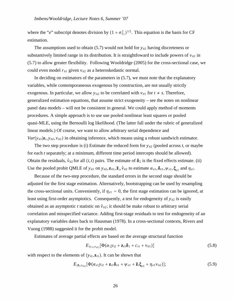
Imbens/Wooldridge, Lecture Notes 6, Summer ’07
where the “e” subscript denotes division by 1 e12 1/2. This equation is the basis for CF
estimation.The assumptions used to obtain (5.7) would not hold for yit2 having discreteness or
substantively limited range in its distribution. It is straightfoward to include powers of vit2 in(5.7) to allow greater flexibility. Following Wooldridge (2005) for the cross-sectional case, wecould even model rit1 given vit2 as a heteroskedastic normal.
In deciding on estimators of the parameters in (5.7), we must note that the explanatoryvariables, while contemporaneous exogenous by construction, are not usually strictlyexogenous. In particular, we allow yis2 to be correlated with vit1 for t ≠ s. Therefore,generalized estimation equations, that assume strict exogeneity – see the notes on nonlinearpanel data models – will not be consistent in general. We could apply method of momentsprocedures. A simple approach is to use use pooled nonlinear least squares or pooledquasi-MLE, using the Bernoulli log likelihood. (The latter fall under the rubric of generalizedlinear models.) Of course, we want to allow arbitrary serial dependence andVaryit1|zi,yit2,vit2 in obtaining inference, which means using a robust sandwich estimator.
The two step procedure is (i) Estimate the reduced form for yit2 (pooled across t, or maybefor each t separately; at a minimum, different time period intercepts should be allowed).Obtain the residuals, vit2 for all i, t pairs. The estimate of 2 is the fixed effects estimate. (ii)Use the pooled probit QMLE of yit1 on yit2,zit1, zi, vit2 to estimate e1,e1,e1,e1 and e1.
Because of the two-step procedure, the standard errors in the second stage should beadjusted for the first stage estimation. Alternatively, bootstrapping can be used by resamplingthe cross-sectional units. Conveniently, if e1 0, the first stage estimation can be ignored, atleast using first-order asymptotics. Consequently, a test for endogeneity of yit2 is easilyobtained as an asymptotic t statistic on vit2; it should be make robust to arbitrary serialcorrelation and misspecified variance. Adding first-stage residuals to test for endogeneity of anexplanatory variables dates back to Hausman (1978). In a cross-sectional contexts, Rivers andVuong (1988) suggested it for the probit model.
Estimates of average partial effects are based on the average structural function
Eci1,vit1 1yt2 zt11 ci1 vit1 (5.8)
with respect to the elements of yt2,zt1. It can be shown that
Ezi,vit2 e1yt2 zt1e1 e1 zie1 e1vit2; (5.9)
26
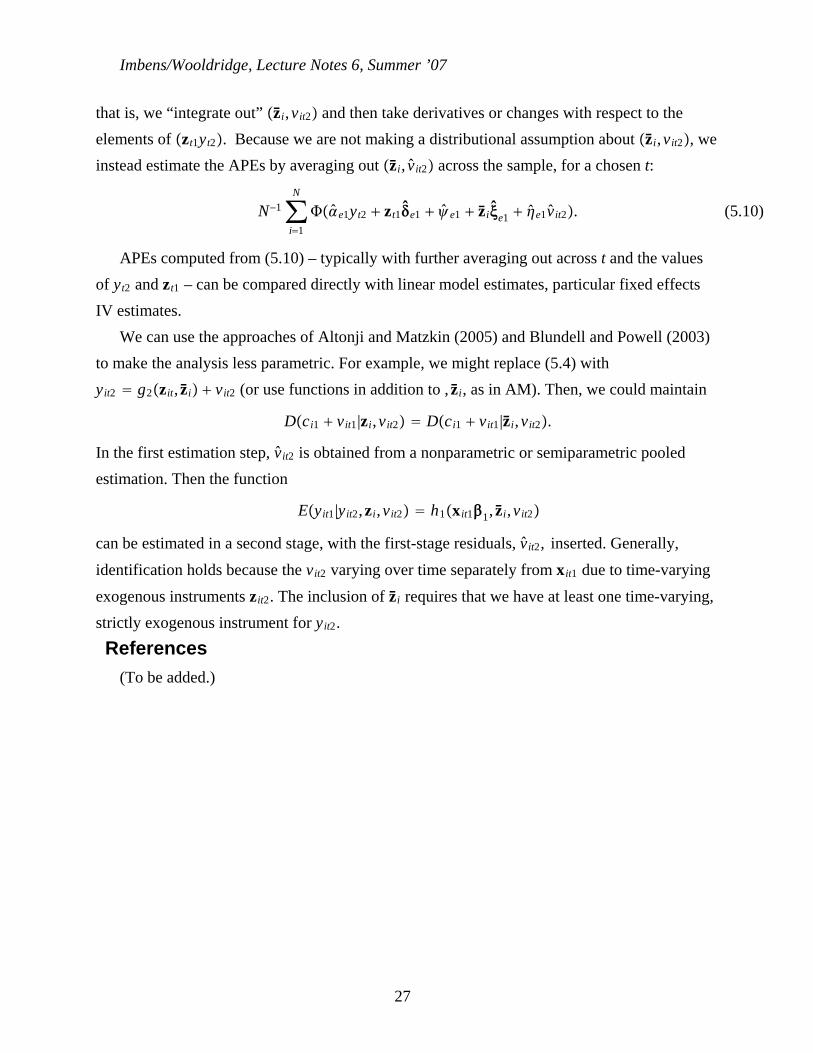
Imbens/Wooldridge, Lecture Notes 6, Summer ’07
that is, we “integrate out” zi,vit2 and then take derivatives or changes with respect to theelements of zt1yt2. Because we are not making a distributional assumption about zi,vit2, weinstead estimate the APEs by averaging out zi, vit2 across the sample, for a chosen t:
N−1∑i1
N
e1yt2 zt1e1 e1 zie1 e1vit2. (5.10)
APEs computed from (5.10) – typically with further averaging out across t and the valuesof yt2 and zt1 – can be compared directly with linear model estimates, particular fixed effectsIV estimates.
We can use the approaches of Altonji and Matzkin (2005) and Blundell and Powell (2003)to make the analysis less parametric. For example, we might replace (5.4) withyit2 g2zit, zi vit2 (or use functions in addition to , zi, as in AM). Then, we could maintain
Dci1 vit1|zi,vit2 Dci1 vit1|zi,vit2.
In the first estimation step, vit2 is obtained from a nonparametric or semiparametric pooledestimation. Then the function
Eyit1|yit2,zi,vit2 h1xit11, zi,vit2
can be estimated in a second stage, with the first-stage residuals, vit2, inserted. Generally,identification holds because the vit2 varying over time separately from xit1 due to time-varyingexogenous instruments zit2. The inclusion of zi requires that we have at least one time-varying,strictly exogenous instrument for yit2.References
(To be added.)
27

Imbens/Wooldridge, Lecture Notes 7, NBER, Summer ’07 1
What’s New in Econometrics NBER, Summer 2007
Lecture 7, Tuesday, July 31th, 11.00-12.30pm
Bayesian Inference
1. Introduction
In this lecture we look at Bayesian inference. Although in the statistics literature ex-
plicitly Bayesian papers take up a large proportion of journal pages these days, Bayesian
methods have had very little impact in economics. This seems to be largely for historial rea-
sons. In many empirical settings in economics Bayesian methods appear statistically more
appropriate, and computationally more attractive, than the classical or frequentist methods
typically used. Recent textbooks discussing modern Bayesian methods with an applied focus
include Lancaster (2004) and Gelman, Carlin, Stern and Rubin (2004).
One important consideration is that in practice frequentist and Baeysian inferences are
often very similar. In a regular parametric model, conventional confidence intervals around
maximum likelihood (that is, the maximum likelihood estimate plus or minus 1.96 times the
estimated standard error), which formally have the property that whatever the true value of
the parameter is, with probability 0.95 the confidence interval covers the true value, can in
fact also be interpreted as approximate Bayesian probability intervals (that is, conditional
on the data and given a wide range of prior distributions, the posterior probability that the
parameter lies in the confidence interval is approximately 0.95). The formal statement of
this remarkable result is known as the Bernstein-Von Mises theorem. This result does not
always apply in irregular cases, such as time series settings with unit roots. In those cases
there are more fundamental differences between Bayesian and frequentist methods.
Typically a number of reasons are given for the lack of Bayesian methods in econometrics.
One is the difficulty in choosing prior distributions. A second reason is the need for a fully
specified parametric model. A third is the computational complexity of deriving posterior
distributions. None of these three are compelling.

Imbens/Wooldridge, Lecture Notes 7, NBER, Summer ’07 2
Consider first the specification of the prior distribution. In regular cases the influence of
the prior distribution disappears as the sample gets large, as formalized in the Bernstein-Von
Mises theorem. This is comparable to the way in which in large samples normal approx-
imations can be used for the finite sample distributions of classical estimators. If, on the
other hand, the posterior distribution is quite sensitive to the choice of prior distribution,
then it is likely that the sampling distribution of the maximum likelihood estimator is not
well approximated by a normal distribution centered at the true value of the parameter in a
frequentist analysis.
A conventional Bayesian analysis does require a fully specified parameter model, as well
as a prior distribution on all the parameters of this model. In frequentist analyses it is
often possible to specify only part of the model, and use a semi-parametric approach. This
advantage is not as clear cut as it may seem. When the ultimate questions of interest do
not depend on certain features of the distribution, the results of a parametric model are
often robust given a flexible specification of the nuisance functions. As a result, extending
a semi-parametric model to a fully parametric one by flexibly modelling the nonparametric
component often works well in practice. In addition, Bayesian semi-parametric methods
have been developed.
Finally, traditionally computational difficulties held back applications of Bayesian meth-
ods. Modern computational advances, in particular the development of markov chain monte
carlo methods, have reduced, and in many cases eliminated, these difficulties. Bayesian anal-
yses are now feasible in many settings where they were not twenty years ago. There are now
few restrictions on the type of prior distributions that can be considered and the dimension
of the models used.
Bayesian methods are especially attractive in settings with many parameters. Examples
discussed in these notes include panel data with individual-level heterogeneity in multiple
parameters, instrumental variables with many instruments, and discrete choice data with
multiple unobserved product characteristics. In such settings, methods that attempt to es-
timate every parameter precisely without linking it to similar parameters, often have poor
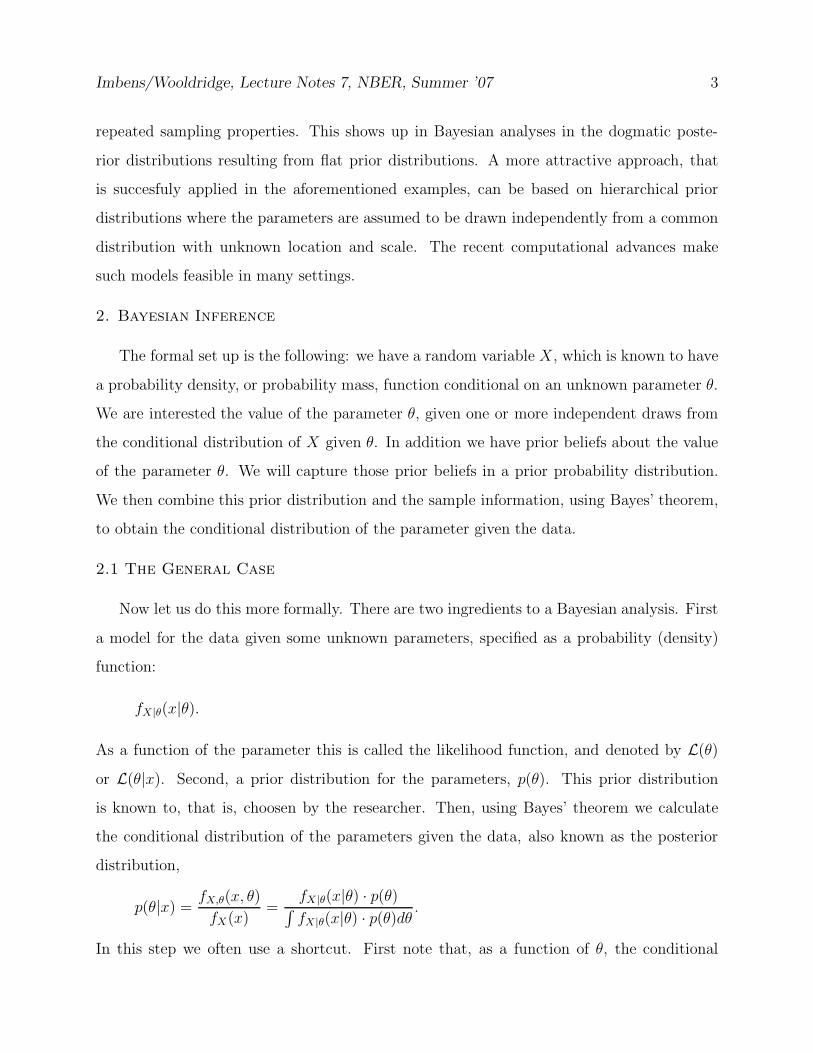
Imbens/Wooldridge, Lecture Notes 7, NBER, Summer ’07 3
repeated sampling properties. This shows up in Bayesian analyses in the dogmatic poste-
rior distributions resulting from flat prior distributions. A more attractive approach, that
is succesfuly applied in the aforementioned examples, can be based on hierarchical prior
distributions where the parameters are assumed to be drawn independently from a common
distribution with unknown location and scale. The recent computational advances make
such models feasible in many settings.
2. Bayesian Inference
The formal set up is the following: we have a random variable X, which is known to have
a probability density, or probability mass, function conditional on an unknown parameter θ.
We are interested the value of the parameter θ, given one or more independent draws from
the conditional distribution of X given θ. In addition we have prior beliefs about the value
of the parameter θ. We will capture those prior beliefs in a prior probability distribution.
We then combine this prior distribution and the sample information, using Bayes’ theorem,
to obtain the conditional distribution of the parameter given the data.
2.1 The General Case
Now let us do this more formally. There are two ingredients to a Bayesian analysis. First
a model for the data given some unknown parameters, specified as a probability (density)
function:
fX |θ(x|θ).
As a function of the parameter this is called the likelihood function, and denoted by L(θ)
or L(θ|x). Second, a prior distribution for the parameters, p(θ). This prior distribution
is known to, that is, choosen by the researcher. Then, using Bayes’ theorem we calculate
the conditional distribution of the parameters given the data, also known as the posterior
distribution,
p(θ|x) =fX,θ(x, θ)
fX(x)=
fX |θ(x|θ) · p(θ)∫
fX |θ(x|θ) · p(θ)dθ.
In this step we often use a shortcut. First note that, as a function of θ, the conditional
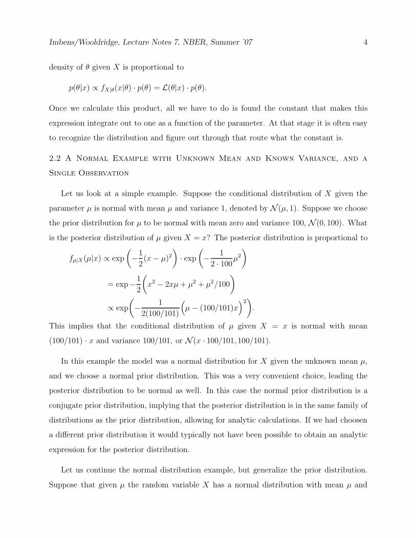
Imbens/Wooldridge, Lecture Notes 7, NBER, Summer ’07 4
density of θ given X is proportional to
p(θ|x) ∝ fX |θ(x|θ) · p(θ) = L(θ|x) · p(θ).
Once we calculate this product, all we have to do is found the constant that makes this
expression integrate out to one as a function of the parameter. At that stage it is often easy
to recognize the distribution and figure out through that route what the constant is.
2.2 A Normal Example with Unknown Mean and Known Variance, and a
Single Observation
Let us look at a simple example. Suppose the conditional distribution of X given the
parameter µ is normal with mean µ and variance 1, denoted by N (µ, 1). Suppose we choose
the prior distribution for µ to be normal with mean zero and variance 100, N (0, 100). What
is the posterior distribution of µ given X = x? The posterior distribution is proportional to
fµ|X(µ|x) ∝ exp
(
−1
2(x− µ)2
)
· exp
(
− 1
2 · 100µ2
)
= exp−1
2
(
x2 − 2xµ + µ2 + µ2/100
)
∝ exp
(
− 1
2(100/101)
(
µ − (100/101)x)2
)
.
This implies that the conditional distribution of µ given X = x is normal with mean
(100/101) · x and variance 100/101, or N (x · 100/101, 100/101).
In this example the model was a normal distribution for X given the unknown mean µ,
and we choose a normal prior distribution. This was a very convenient choice, leading the
posterior distribution to be normal as well. In this case the normal prior distribution is a
conjugate prior distribution, implying that the posterior distribution is in the same family of
distributions as the prior distribution, allowing for analytic calculations. If we had choosen
a different prior distribution it would typically not have been possible to obtain an analytic
expression for the posterior distribution.
Let us continue the normal distribution example, but generalize the prior distribution.
Suppose that given µ the random variable X has a normal distribution with mean µ and
Imbens/Wooldridge, Lecture Notes 7, NBER, Summer ’07 5
known variance σ2, or N (µ, σ2). The prior distribution for µ is normal with mean µ0 and
variance τ 2, or N (µ0, τ2). Then the posterior distribution is proportional to:
fµ|X(µ|x) ∝ exp
(
− 1
2σ2(x − µ)2
)
· exp
(
− 1
2 · τ 2(µ − µ0)
2
)
∝ exp−1
2
(
x2
σ2− 2xµ
σ2+
µ2
σ2+
µ2
τ 2− 2µµ0
τ 2+
µ20
τ 2
)
∝ exp−1
2
(
µ2σ2 + τ 2
τ 2σ2− µ
2xτ 2 + 2µ0σ2
τ 2 · σ2
)
∝ exp− 1
2(1/(1/τ 2 + 1/σ2))
(
(µ − (x/σ2 + µ0/τ2)/(1/σ2 + 1/τ 2)
)
∼ N(
x/σ2 + µ0/τ2
1/σ2 + 1/τ 2,
1
1/τ 2 + 1/σ2)
)
.
The result is quite intuitive: the posterior mean is a weighted average of the prior mean
µ0 and the observation x with weights adding up to one and proportional to the precision
(defined as one over the variance), 1/σ2 for x and 1/τ 2 for µ0:
E[µ|X = x] =xσ2 + µ0
τ2
1
σ2 + 1
τ2
.
The posterior precision is obtained by adding up the precision for each component
1
V(µ|X)=
1
σ2+
1
τ 2.
So, what you expect ex post, E[µ|X], that is, after seeing the data, is a weighted average
of what you expected before seeing the data, E[µ] = µ0, and the observation, X, with the
weights determined by their respective variances.
There are a number of insights obtained by studying this example more carefully. Suppose
we are really sure about the value of µ before we conduct the experiment. In that case we
would set τ 2 small and the weight given to the observation would be small, and the posterior
distribution would be close to the prior distribution. Suppose on the other hand we are
very unsure about the value of µ. What value for τ should we choose? Obviously a large
value, but what is the limit? We can in fact let τ go to infinity. Even though the prior
distribution is not a proper distribution anymore if τ 2 = ∞, the posterior distribution is
Imbens/Wooldridge, Lecture Notes 7, NBER, Summer ’07 6
perfectly well defined, namely µ|X ∼ N (X, σ2). In that case we have an improper prior
distribution. We give equal prior weight to any value of µ. That would seem to capture
pretty well the idea that a priori we are ignorant about µ. This is the idea of looking for
an relatively uninformative prior distribution. This is not always easy, and the subject of
a large literature. For example, a flat prior distribution is not always uninformative about
particular functions of parameters.
2.3 A Normal Example with Unknown Mean and Known Variance and Mul-
tiple Observations
Now suppose we have N independent draws from a normal distribution with unknown
mean µ and known variance σ2. Suppose we choose, as before, the prior distribution to be
normal with mean µ0 and variance τ 2, or N (µ0, τ2).
The likelihood function is
L(µ|σ2, x1, . . . , xN ) =
N∏
i=1
1√2πσ2
exp
(
− 1
2σ2(xi − µ)2
)
,
so that with a normal (µ0, τ2) prior distribution the posterior distribution is proportional to
p(µ|x1, . . . , xN ) ∝ exp
(
− 1
2τ 2(µ − µ0)
2
)
·N∏
i=1
exp
(
− 1
2σ2(xi − µ)2
)
.
Thus, with N observations x1, . . . , xN we find, after straightforward calculations,
µ|X1, . . . , XN ∼ N(
µ0/τ2 +
∑
xi/σ2
1/τ 2 + N/σ2,
1
1/τ 2 + N/σ2
)
.
2.4 The Normal Distribution with Known Mean and Unknown Variance
Let us also briefly look at the case of a normal model with known mean and unknown
variance. Thus,
Xi|σ2 ∼ N (0, σ2),
and X1, . . . , XN independent given σ2. The likelihood function is
L(σ2) =N∏
i=1
σ−N exp
(
− 1
2σ2X2
i
)
.
Imbens/Wooldridge, Lecture Notes 7, NBER, Summer ’07 7
Now suppose that the prior distribution for σ2 is, for some fixed S20
and K0, such that the
distribution of σ−2 · S20 · K0 is chi-squared with K0 degrees of freedom. In other words, the
prior distribution of σ−2 is (S20 · K0)
−1 times a chi-squared distribution with K0 degrees of
freedom. Then the posterior distribution of σ−2 is (S20· K0 +
∑
i X2i )−1 times a chi-squared
distribution with K0 + N degrees of freedom, so this is a conjugate prior distribution.
3. The Bernstein-Von Mises Theorem
Let us go back to the normal example with N observations, and unknown mean and
known variance. In that case with a normal N (µ0, τ2) prior distribution the posterior for µ
is
µ|x1, . . . , xN ∼ N(
x · 1
1 + σ2/(N · τ 2)+ µ0 ·
σ2/(Nτ 2)
1 + σ2/(Nτ 2),
σ2/N
1 + σ2/(Nτ 2)
)
.
When N is very large, the distribution of√
N (µ−x) conditional on the data is approximately
√N (x− µ)|x1, . . . , xN ∼ N (0, σ2).
In other words, in large samples the influence of the prior distribution disappears, unless
the prior distribution is choosen particularly badly, e.g., τ 2 equal to zero. This is true in
general, i.e., for different models and different prior distributions. Moreover, in a frequentist
analysis we would find that in large samples (and in this specific normal example even in
finite samples),
√N (x− µ)|µ ∼ N (0, σ2).
Let us return to the Bernoulli example to see the same point. Suppose that conditional on
the parameter P = p, the random variables X1, X2, . . . , XN are independent with Bernoulli
distributions with probability p. Let the prior distribution of P be Beta with parameters α
and β, or B(α, β). Now consider the conditional distribution of P given X1, . . . , XN :
fP |X1,...,XN(p|x) ∝ pα−1+
P
N
i=1Xi · (1 − p)β−1+N−
P
N
i=1Xi,
which is a Beta distribution, B(α − 1 +∑N
i=1Xi, β − 1 + N − ∑N
i=1Xi), with mean and
Imbens/Wooldridge, Lecture Notes 7, NBER, Summer ’07 8
variance
E[P |X1, . . . , XN ] =α +
∑N
i=1Xi
α + β + N, and V(P ) =
(α +∑N
i=1Xi)(β + N − ∑N
i=1Xi)
(α + β + N)2(α + β + 1 + N).
What happens if N gets large? Let p =∑
i Xi/N be the relative frequency of success (which
is the maximum likelihood estimator for p). Then the mean and variance converge to
E[P |X1, . . . , XN ] ≈ p,
and
V(P ) ≈ 0.
As the sample size gets larger, the posterior distribution becomes concentrated at a value
that does not depend on the prior distribution. This in fact can be taken a step further.
In this example, the limiting distribution of√
N · (P − p) conditional on the data, can be
shown to be
√N (p − P |x1, . . . , xN
d−→ N (0, p(1 − p)),
again irrespective of the choice of α and β. The interpretation of this result is very impor-
tant: in large sample the choice of prior distribution is not important in the sense that the
information in the prior distribution gets dominated by the sample information. That is,
unless your prior beliefs are so strong that they cannot be overturned by evidence (i.e., the
prior distribution is zero over some important range of the parameter space), at some point
the evidence in the data outweights any prior beliefs you might have started out with.
This is known as the Bernstein-von Mises Theorem. Here is a general statement for the
scalar case. Let the information matrix Iθ at θ:
Iθ = −E
[
∂2
∂θ∂θ′ln fX(x|θ)
]
= −∫
∂2
∂θ∂θ′ln fX(x|θ)fX(x|θ)dx,
and let σ2 be the inverse at a fixed value θ0.
σ2 = I−1
θ0.
Imbens/Wooldridge, Lecture Notes 7, NBER, Summer ’07 9
Let p(θ) be the prior distribution, and pθ|X1,...,XN(θ|X1, . . . , XN ) be the posterior distribution.
Now let us look at the distribution of a transformation of θ, γ =√
N(θ − θ0), with density
pγ|X1,...,XN(γ|X1, . . . , XN ) = pθ|X1,...,XN
(θ0 +√
N ·γ|X1, . . . , XN )/√
N . Now let us look at the
posterior distribution for θ if in fact the data were generated by f(x|θ) with θ = θ0. In that
case the posterior distribution of γ converges to a normal distribution with mean zero and
variance equal to σ2 in the sense that
supγ
∣
∣
∣
∣
pγ|X1,...,XN(γ|X1, . . . , XN ) − 1√
2πσ2exp
(
− 1
2σ2γ2
)∣
∣
∣
∣
−→ 0.
See Van der Vaart (2001), or Ferguson (1996). At the same time, if the true value is θ0, then
the mle θmle also has a limiting distribution with mean zero and variance σ2:
√N (θml − θ0)
d−→ N (0, σ2).
The implication is that we can interpret confidence intervals as approximate probability
intervals from a Bayesian perspective. Specifically, let the 95% confidence interval be [θml −1.96 · σ/
√N, θml + 1.96 · σ/
√N ]. Then, approximately,
Pr(
θml − 1.96 · σ/√
N ≤ θ ≤ θml + 1.96 · σ/√
N∣
∣
∣X1, . . . , XN
)
−→ 0.95.
There are important cases where this result does not hold, typically when convergence
to the limit distribution is not uniform. One is the unit-root setting. In a simple first
order autoregressive example it is still the case that with a normal prior distribution for the
autoregressive parameter the posterior distribution is normal (see Sims and Uhlig, 1991).
However, if the true value of the autoregressive parameter is unity, the sampling distribution
is not normal even in large samples. In that case one has to take a more principled stand
whether one wants to make subjective probability statements, or frequentist claims.
4. Markov Chain Monte Carlo Methods
Are we really restricted to choosing the prior distributions in these conjugate families as
we did in the examples so far? No. The posterior distributions are well defined irrespective
of conjugacy. Conjugacy only simplifies the computations. If you are outside the conjugate
Imbens/Wooldridge, Lecture Notes 7, NBER, Summer ’07 10
families, you typically have to resort to numerical methods for calculating posterior moments.
Recently many methods have been developed that make this process much easier, including
Gibbs sampling, Data Augmentation, and the Metropolis-Hastings algorithm. All three are
examples of M arkov-Chain-Monte-Carlo or MCMC methods.
The general idea is to construct a chain, or sequence of values, θ0, θ1, . . . , such that for
large k θk can be viewed as a draw from the posterior distribution of θ given the data. This
is implemented through an algorithm that, given a current value of the parameter vector θk,
and given the data X1, . . . , XN draws a new value θk+1 from a distribution f(·) indexed by
θk and the data:
θk+1 ∼ f(θ|θk, data),
in such a way that if the original θk came from the posterior distribution, then so does θk+1
(although θk and θk+1 in general will not be independent draws)
θk|data ∼ p(θ|data), then θk+1|data ∼ p(θ|data).
Even if we have such an algorithm, the problem is that in principle we would need a starting
value θ0 that such that
θ0 ∼ p(θ|data).
However, in many cases, irrespective of where we start, that is, irrespective of θ0, as k −→ ∞,
it will be the case that the distribution of the parameter conditional only on the data
converges to the posterior distribution:
θk|datad−→ p(θ|data),
as k −→ ∞.
If that is true, then we can just pick a θ0, run the chain for a long time, collect the
values θ0, . . . , θK for a large value of K, and approximate the posterior distribution by the
distribution of θK0, . . . , θK . For example, the mean and standard deviation of the posterior
Imbens/Wooldridge, Lecture Notes 7, NBER, Summer ’07 11
distribution would be estimated as
E[θ|data] =1
K − K0 + 1
K∑
k=K0
θk,
and
V[θ|data] =1
K −K0 + 1
K∑
k=K0
(
θk − E[θ|data])2
.
The first K0 − 1 iterations are discarded to let algorithm converge to the stationary distri-
bution, or “burn in.”
4.1 Gibbs Sampling
The idea being the Gibbs sampler is to partition the vector of parameters θ into two (or
more) parts, θ′ = (θ′1, θ′2). Instead of sampling θk+1 directly from a conditional distribution
of
f(θ|θk, data),
we first sample θ1,k+1 from the conditional distribution of
p(θ1|θ2,k, data),
and then sample θ2,k+1 from the conditional distribution of
p(θ2|θ1,k+1, data).
It is clear that if (θ1,k, θ2,k) is from the posterior distribution, then so is (θ1,k, θ2,k).
4.2 Data Augmentation
This is best illustrated with an example. Suppose we are interested in estimating the
parameters of a censored regression or Tobit model. There is a latent variable
Y ∗i = X ′
iβ + εi,
with εi|Xi ∼ N (0, 1). (I assume the variance is known for simplicity. This is not essential).
We observe
Yi = max(0, Y ∗i ),
Imbens/Wooldridge, Lecture Notes 7, NBER, Summer ’07 12
and the regressors Xi. Suppose the prior distribution for β is normal with some mean µ,
and some covariance matrix Ω.
The posterior distribution for β does not have a closed form expression. This is not due
to an awkward choice for the prior distribution, because there is no conjugate family for this
problem. There is however a simple way of obtaining draws from the posterior distribution
using data augmentation in combination with the Gibbs sampler. The first key insight is to
view both the vector Y∗ = (Y ∗1 , . . . , Y ∗
N) and β as unknown random variables. The Gibbs
sampler consists of two steps. First we draw all the missing elements of Y∗ given the current
value of the parameter β, say βk. This involves drawing a series of truncated univariate
normal random variables:
Y ∗i |β, data ∼ T N (X ′
iβ, 1, 0) ,
if observation i is truncated, where T N (µ, σ2, c) denotes a truncated normal distribution
with mean and variance (for the not truncated normal distribution) µ and σ2, and truncation
point c (truncated from above). (Note that we do not need to draw the observed values of
Y ∗i .) Second, we draw a new value for the parameter, βk+1 given the data and given the
(partly drawn) Y∗. The latter is easy given the normal prior distribution: the posterior is
normal:
p (β|data,Y∗) ∼ N(
(
X′X + Ω−1)−1 ·
(
X′Y + Ω−1µ)
,(
X′X + Ω−1)−1
)
.
In this example it would still have been feasible to do evaluate the likelihood function di-
rectly using numerical integration. Another example where the computational advantages
of using data augmentation are even more striking is the multinomial probit model with an
unrestricted covariance matrix. See Rossi, Allenby and McCulloch (2005).
4.3 Metropolis-Hastings
We are again interested in p(θ|data). In this case p(θ|data) is assumed to be easy to
evaluate, but difficult to draw from. Suppose we have a current value θk. Then we draw a new
candidate value for the chain from a candidate distribution q(θ|θk, data). This distribution
Imbens/Wooldridge, Lecture Notes 7, NBER, Summer ’07 13
may (but need not) depend on θk. Denote the candidate value by θ. We will either accept
the new value, or keep the old value. Then we calculate the ratio
r(θk, θ) =p(θ|data) · q(θk|θ, data)
p(θk|data) · q(θ|θk, data).
The probability that the new draw θ is accepted is
ρ(θk, θ) = min (1, r(θk, θ)) ,
so that
Pr (θk+1 = θ) = ρ(θk, θ), and Pr (θk+1 = θk) = 1 − ρ(θk, θ).
The optimal choice for the candidate distribution is
q∗(θ|θk, data) = p(θ|data),
so that ρ(θk, θ) = 1 and every draw will get accepted. The trouble is that it is difficult to
draw from this distribution. In practice you want to have a relatively dispersed distribution
as the candidate distribution, so that the ratio r(θk, θ) does not get too large.
5. Examples
Here we discuss a number of applications of Bayesian methods. All models contain
parameters that are difficult to estimate consistently, and in all cases numerical methods are
required to obtain draws from the posterior distribution. The first two are about random
coeffiecients. In that case Bernstein-Von Mises would only apply to the individual level
parameters if the number of observations per individual would get large.
5.1 Demand Models with Unobserved Heterogeneity in Preferences
Rossi, McCulloch, and Allenby (1996, RMA) are interested in the optimal design of
coupon policies. Supermarkets can choose to offer identical coupons for a particular product
(tuna cans is the example they use). Alternatively, they may choose to offer differential
coupons based on consumer’s fixed characteristics. Taking this ever further, they could make
the value of the coupon a function of the purchase history of the individual, for example
Imbens/Wooldridge, Lecture Notes 7, NBER, Summer ’07 14
tailoring the amount of the discount offered in the coupon to the evidence for price sensitivity
contained in purchase patterns. RMA set out to estimate the returns to various coupon
policies. It is clear that for this investigation to be meaningful one needs to allow for
household-level heterogeneity in taste parameters and price elasticities. Even with large
amounts of data available, there will be many households for whom these parameters cannot
be estimated precisely. RMA therefore use a hieararchical or random coefficients model.
RMA model households choosing the product with the highest utility, where utility for
household i, product j, j = 0, 1, . . . , J , at purchase time t is
Uijt = X ′itβi + εijt,
with the εijt independent accross households, products and purchase times, and normally
distributed with product-specific variances σ2j (and σ2
0normalized to one). The Xit are
observed choice characteristics that in the RMA application include price, some marketing
variables, as well as brand dummies. All choice characteristics are assumed to be exogenous,
although that assumption may be questioned for the price and marketing variables. Because
for some households we have few purchases, it is not possible to accurately estimate all βi
parameters. RMA therefore assume that the household-specific taste parameters are random
draws from a normal distribution centered at Z ′iΓ:
βi = Z ′iΓ + ηi, ηi ∼ N (0, Σ).
Now Gibbs sampling can be used to obtain draws from the posterior distribution of the βi.
To be a little more precise, let us describe the steps in the Gibbs sampler for this example.
For more details see RMA. RMA use a normal prior distribution for Γ, a Wishart prior
distribution for Σ−1, and inverse Gamma prior distributions for the σ2j . To implement the
Gibbs sampler, the key is to treat the unobserved utilities as parameters.
The first step is to draw the household parameters βi given the utilities Uijt and the
common parameters Γ, Σ, and σ2j . This is straightforward, because we have a standard
normal linear model for the utilities, with a normal prior distribution for βi with parameters

Imbens/Wooldridge, Lecture Notes 7, NBER, Summer ’07 15
Z ′iΓ and variance Σ, and Ti observations. We can draw from this posterior distribution for
each household i.
In the second step we draw the σ2j using the results for the normal distribution with
known mean and unknown variance.
The third step is to draw from the posterior of Γ and Σ, given the βi. This again is just
a normal linear model, now with unknown mean and unknown variance.
The fourth step is to draw the unobserved utilities given the βi and the data. Doing
this one household/choice at a time, conditioning on the utilities for the other choices, this
merely involves drawing from a truncated normal distribution, which is simple and fast.
For some households, those with many recorded purchases and sufficient variation in
product characteristics, the posterior distribution will be tight, whereas for others there may
be little information in the data and the posterior distribution, conditional on the data as
well as Γ and Σ, will essentially be the prior distribution for βi, which is N (Z ′iΓ, Σ).
To think about optimal coupon policies given a particular information set it is useful
to think first about the posterior distribution of the household specific parameters βi. If
a supermarket had full information about the household parameters βi, there would be no
additional value in the household characteristics or the purchase history. When we therefore
compare a blanket coupon policy (where every household would receive a coupon with the
same value) with one that depends on a larger information set that household demographics,
or one that also includes purchase histories, the key question is how much precision the
information adds about the household level parameters. Specifically, how does the marginal
distribution of the household parameters compare with the conditional distribution given
purchase histories or given demographics. To make this specific, suppose that the there is
only one choice characteristic, price, with household parameter βi.
The starting point is the case with no household information whatsoever. We can simulate
draws from this distribution by drawing from the conditional distribution of βi given the data
for randomly selected households. In the second case we allow conditioning on the household
Imbens/Wooldridge, Lecture Notes 7, NBER, Summer ’07 16
demographic characteristics Zi. This leads to less dispersed posterior distributions for the
price coefficients. In the third case we also condition on purchase histories. Figure 1, taken
from RMA shows for ten households the boxplots of the posterior distribution of the price
coefficient under these information sets, one can see the increased precision that results from
conditioning on the purchase histories.
5.2 Panel Data Models with Multiple Individual Specific Parameters
Chamberlain and Hirano (1999, CH), see also Hirano (2002), are interested in deriving
predictive distributions for earnings using longitudinal data. They are particularly interested
in allowing for unobserved individual-level heterogeneity in earnings variances. The specific
model they use assumes that log earnings Yit follow the process
Yit = X ′iβ + Vit + αi + Uit/hi.
The key innovation in the CH study is the individual variation in the conditional variance,
captured by hi. In this specification X ′iβ is a systematic component of log earnings, similar
to that in specifications used in Abowd and Card () (CH actually use a more general non-
linear specification, but the simpler one suffices for the points we make here.) The second
component in the model, Vit, is a first order autoregressive component,
Vit = γ · Vit−1 + Wit,
where
Vi1 ∼ N (0, σ2
v), Wit ∼ N (0, σ2
w).
The first factor in the last component has a standard normal distribution,
Uit ∼ N (0, 1).
Analyzing this model by attempting to estimate the αi and hi directly would be misguided.
From a Bayesian perspective this corresponds to assuming a flat prior distribution on a
high-dimensional parameter space.
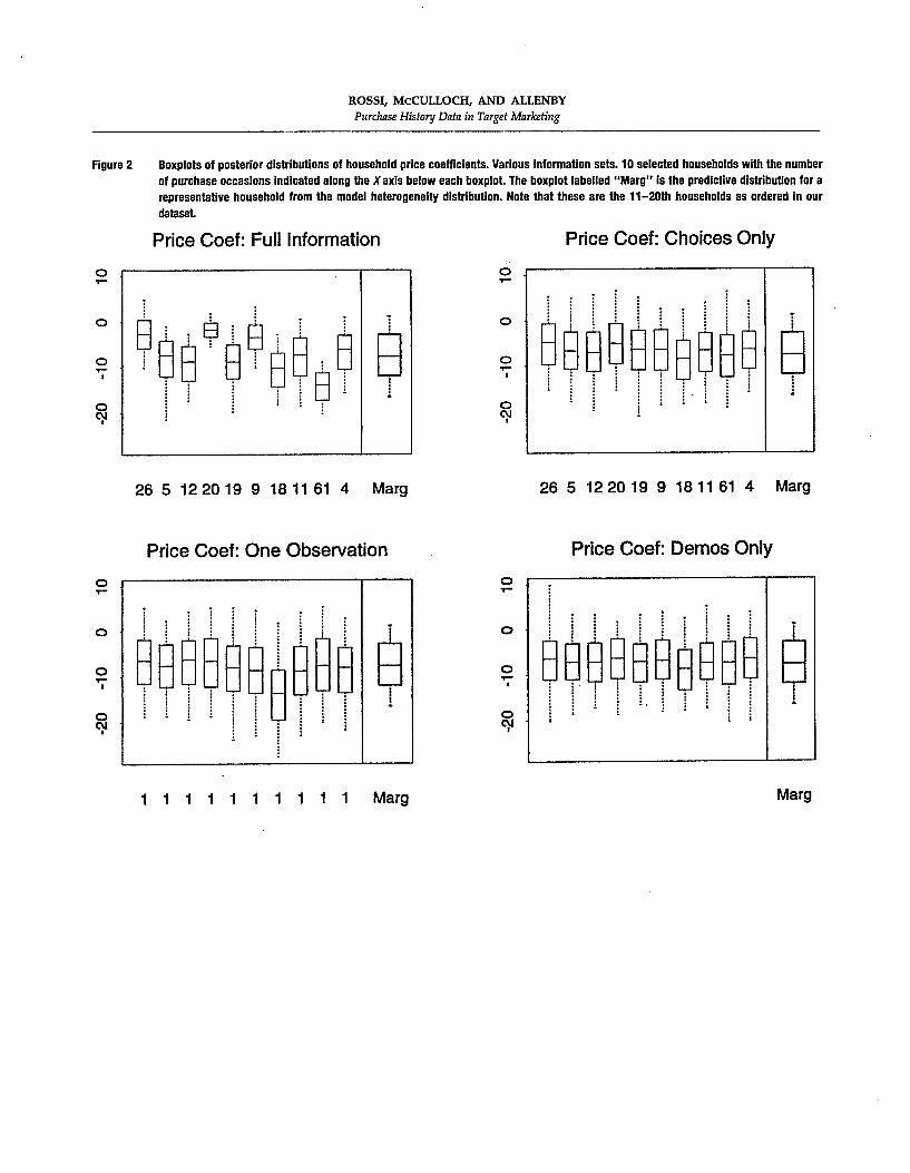

Imbens/Wooldridge, Lecture Notes 7, NBER, Summer ’07 17
To avoid such pitfalls CH model αi and hi through a random effects specification.
αi ∼ N (0, σ2
α). and hi ∼ G(m/2, τ/2).
In their empirical application using data from the Panel Study of Income Dynamics (PSID),
CH find strong evidence of heterogeneity in conditional variances. Some of this heterogeneity
is systematically associated with observed characteristics of the individual such as educa-
tion, with higher educated individuals experiences lower levels of volatility. Much of the
heterogeneity, however, is within groups homogenous in observed characteristics.
The following table, from CH, presents quantiles of the predictive distribution of the
conditional standard deviation 1/√
hi for different demographic groups: Up to here one
Table 1: quantiles of the predictive distribution of the conditional standarddeviation
QuantileSample 0.05 0.10 0.25 0.50 0.75 0.90 0.95
All (N=813) 0.04 0.05 0.07 0.11 0.20 0.45 0.81High School Dropouts (N=37) 0.06 0.08 0.11 0.16 0.27 0.49 0.79High School Graduates (N=100) 0.04 0.05 0.06 0.11 0.21 0.49 0.93College Graduates (N=122) 0.03 0.04 0.05 0.09 0.18 0.40 0.75
could have done essentially the same using frequentist methods. One could estimate first the
common parameters of the model, β, σ2v, σ2
w, m, τ , and σ2α by maximum likelihood given the
specification of the model. Conditional on the covariates one could for each demographic
group write the quantiles of the conditional standard deviation in terms of these parameters
and obtain point estimates for them.
However, CH wish to go beyond this and infer individual-level predictive distributions
for earnings. Taking a particular individual, one can derive the posterior distribution of
αi, hi, β, σ2v, and σ2
w, given that individual’s earnings as well as other earnings, and predict
future earnings. To illustrate this CH report earnings predictions for a number of individuals.
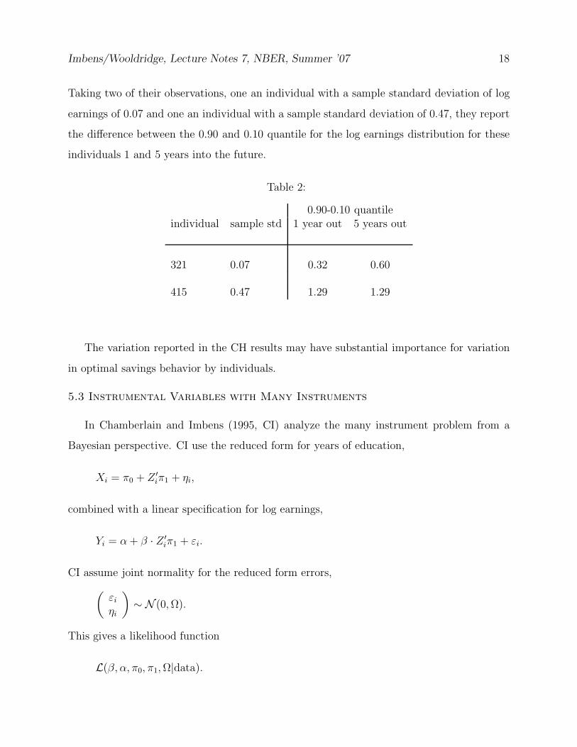
Imbens/Wooldridge, Lecture Notes 7, NBER, Summer ’07 18
Taking two of their observations, one an individual with a sample standard deviation of log
earnings of 0.07 and one an individual with a sample standard deviation of 0.47, they report
the difference between the 0.90 and 0.10 quantile for the log earnings distribution for these
individuals 1 and 5 years into the future.
Table 2:
0.90-0.10 quantileindividual sample std 1 year out 5 years out
321 0.07 0.32 0.60
415 0.47 1.29 1.29
The variation reported in the CH results may have substantial importance for variation
in optimal savings behavior by individuals.
5.3 Instrumental Variables with Many Instruments
In Chamberlain and Imbens (1995, CI) analyze the many instrument problem from a
Bayesian perspective. CI use the reduced form for years of education,
Xi = π0 + Z ′iπ1 + ηi,
combined with a linear specification for log earnings,
Yi = α + β · Z ′iπ1 + εi.
CI assume joint normality for the reduced form errors,
(
εi
ηi
)
∼ N (0, Ω).
This gives a likelihood function
L(β, α, π0, π1, Ω|data).
Imbens/Wooldridge, Lecture Notes 7, NBER, Summer ’07 19
The focus of the CI paper is on inference for β, and the sensitivity of such inferences to the
choice of prior distribution in settings with large numbers of instruments. In that case the
dimension of the parameter space is high. Hence a flat prior distribution may in fact be a
poor choice. One way to illustrate see this is that a flat prior on π1 leads to a prior on the
sum∑K
k=1π2
ik that puts most probability mass away from zero. If in fact the concern is that
collectively, the instruments are all weak, one should allow for this possibility in the prior
distribution. To be specific, if the prior distribution for the π1k is dispersed, say N (0, 1002),
then the prior distribution for the∑
i π21k is 100 times a chi-squared random variable with
degrees of freedom equal to K, implying that a priori the concentration parameter is known
to be large.
CI then show that the posterior distribution for β, under a flat prior distribution for
π1 provides an accurate approximation to the sampling distribution of the TSLS estimator,
providing both a further illustration of the lack of appeal of TSLS in settings with many
instruments, and the unattractiveness of the flat prior distribution.
As an alternative CI suggest a hierarchical prior distribution with
π1k ∼ N (µπ, σ2
π).
In the Angrist-Krueger 1991 compulsory schooling example there is in fact a substantive
reason to believe that σ2π is small. If the π1k represent the effect of the differences in the
amount of required schooling, one would expect the magnitude of the π1k to be less than the
amount of variation in the compulsory schooling. The latter is less than one year. Since any
distribution with support on [0, 1] has a variance less than or equal to 1/12, the standard
deviation of the first stage coefficients should not be more than√
1/12 = 0.289. Using the
Angrist-Krueger data CI find that the posterior distribution for σπ is concentrated close to
zero, with the posterior mean and median equal to 0.119.
5.4 Binary Response with Endogenous Discrete Regressors
Geweke, Gowrisankaran, and Town (2003, GGT) are interested in estimating the effect of
hospital quality on mortality, taking into account possibly non-random selection of patients
Imbens/Wooldridge, Lecture Notes 7, NBER, Summer ’07 20
into hospitals. Patients can choose from 114 hospitals. Given their observed individual
characteristics Zi, latent mortality is
Y ∗i =
113∑
j=1
Cijβj + Z ′iγ + εi,
where Cij is an indicator for patient i going to hospital j. The focus is on the hospital effects
on mortality, βj. Realized mortality is
Yi = 1Y ∗i ≥ 0.
The concern is about selection into the hospitals, and the possibility that this is related to
unobserved components of latent mortality GGT model latent the latent utility for patient
i associated with hospital j as
C∗ij = X ′
ijα + ηij,
where the Xij are hospital-individual specific characteristics, including distance to hospital.
Patient i then chooses hospital j if
C∗ij ≥ Cik, for k = 1, . . . , 114.
The endogeneity is modelled through the potential correlation between ηij and εi. Specifi-
cally, GGT asssume that as
εi =
113∑
j=1
ηij · δj + ζi,
where the ζi is a standard normal random variable, independent of the other unobserved
components. GGT model the ηij as standard normal, independent across hospitals and
across individuals. This is a very strong assumption, implying essentially the independence
of irrelevant alternatives property. One may wish to relax this by allowing for random
coefficients on the hospital characteristics.
Given these modelling decisions GGT have a fully specified joint distribution of hospi-
tal choice and mortality given hospital and individual characteristics. The log likelihood
Imbens/Wooldridge, Lecture Notes 7, NBER, Summer ’07 21
function is highly nonlinear, and it is unlikely it can be well approximated by a quadratic
function. GGT therefore use Bayesian methods, and in particular the Gibbs sampler to ob-
tain draws from the posterior distribution of interest. In their empirical analysis GGT find
strong evidence for non-random selection. They find that higher quality hospitals attract
sicker patients, to the extent that a model based on exogenous selection would have led to
misleading conclusions on hospital quality.
5.5 Discrete Choice Models with Unobserved Choice Characteristics
Athey and Imbens (2007, AI) study discrete choice models, allowing both for unobserved
individual heterogeneity in taste parameters as well as for multiple unobserved choice charac-
teristics. In such settings the likelihood function is multi-modal, and frequentist approxima-
tions based on quadratic approximations to the log likelihood function around the maximum
likelihood estimator are unlikely to be accurate. The specific model AI use assumes that the
utility for individual i in market t for choice j is
Uijt = X ′itβi + ξ′jγi + εijt,
where Xit are market-specific observed choice characteristics, ξj is a vector of unobserved
choice characteristics, and εijt is an idiosyncratic error term, independent accross market,
choices, and individuals, with a normal distribution centered at zero, and with the variance
normalized to unity. The individual-specific taste parameters for both the observed and
unobserved choice characteristics normally distributed:
(
βi
γi
)
|Zi ∼ N (∆Zi, Ω),
with the Zi observed individual characteristics.
AI specify a prior distribution on the common parameters, ∆, and Ω, and on the values of
the unobserved choice characteristics ξj . Using gibbs sampling and data augmentation with
the unobserved utilities as unobserved random variables makes sampling from the posterior
distribution conceptually straightforward even in cases with more than one unobserved choice
characteristic. In contrast, earlier studies using multiple unobserved choice characteristics

Imbens/Wooldridge, Lecture Notes 7, NBER, Summer ’07 22
(Elrod and Keane, 1995; Goettler and Shachar, 2001), using frequentist methods, faced much
heavier computational burdens.
Imbens/Wooldridge, Lecture Notes 7, NBER, Summer ’07 23
References
Athey, S., and G. Imbens, (2007), “Discrete Choice Models with Multiple Unobserved
Product Characteristics,” International Economic Review, forthcoming.
Box, G., and G. Tiao, (1973), Bayesian Inference in Statistical Analysis, Wiley, NY.
Chamberlain, G., and K. Hirano, (1996), “Hirearchical Bayes Models with Many
Instrumental Variables,” NBER Technical Working Paper 204.
Chamberlain, G., and G. Imbens, (1999), “Predictive Distributions based on Lon-
gitudinal Eearnings Data,” Annales d’Economie et de Statistique, 55-56, 211-242.
Elrod, T., and M. Keane, (1995), “A Factor-Analytic Probit Model for Representing
the Market Structure in Panel Data, ”Journal of Marketing Research, Vol. XXXII, 1-16.
Ferguson, T., (1996), A Course in Large Sample Theory, Chapman and Hall, new
York, NY.
Gelman, A., J. Carlin, H. Stenr, and D. Rubin, (2004), Bayesian Data Analysis,
Chapman and Hall, New York, NY.
Gelman, A., and J. Hill, (2007), Data Analysis Using Regression and Multilevel/Hierarchical
Models, Cambridge University Press.
Geweke, J., G. Gowrisankaran, and R. Town, (2003), “Bayesian Inference for
Hospital Quality in a Selection Model,” Econometrica, 71(4), 1215-1238.
Geweke, J., (1997), “Posterior Simulations in Econometrics,” in Advances in Economics
and Econometrics: Theory and Applications, Vol III, Kreps and Wallis (eds.), Cambridge
University Press.
Gilks, W. S. Richardson and D. Spiegelhalter, (1996), Markvo Chain Monte
Carlo in Practice, Chapman and Hall, New York, NY.
Goettler, J., and R. Shachar (2001), “Spatial Competition in the Network Televi-
Imbens/Wooldridge, Lecture Notes 7, NBER, Summer ’07 24
sion Industry,” RAND Journal of Economics, Vol. 32(4), 624-656.
Lancaster, T., (2004), An Introduction to Modern Bayesian Econometrics, Blackwell
Publishing, Malden, MA.
Rossi, P., R. McCulloch, and G. Allenby, (1996), “The Value of Purchasing
History Data in Target Marketing,” Marketing Science, Vol 15(4), 321-340.
Rossi, P., G. Allbeny, and R. McCulloch, (2005), Bayesian Statistics and Mar-
keting, Wiley, Hoboken, NJ.
Sims, C., and H. Uhlig, (1991), “Understanding Unit Rotters: A Helicopter View,”
Econometrica, 59(6), 1591-1599.
Imbens/Wooldridge, Lecture Notes 8, Summer ’07
What’s New in Econometrics? NBER, Summer 2007Lecture 8, Tuesday, July 31st, 2.00-3.00 pm
Cluster and Stratified SamplingThese notes consider estimation and inference with cluster samples and samples obtained
by stratifying the population. The main focus is on true cluster samples, although the case ofapplying cluster-sample methods to panel data is treated, including recent work where the sizesof the cross section and time series are similar. Wooldridge (2003, extended version 2006)contains a survey, but some recent work is discussed here.1. THE LINEAR MODEL WITH CLUSTER EFFECTS
This section considers linear models estimated using cluster samples (of which a panel dataset is a special case). For each group or cluster g, let ygm,xg, zgm : m 1, . . . ,Mg be the
observable data, where Mg is the number of units in cluster g, ygm is a scalar response, xg is a
1 K vector containing explanatory variables that vary only at the group level, and zgm is a
1 L vector of covariates that vary within (as well as across) groups.1.1 Specification of the Model
The linear model with an additive error is
ygm xg zgm vgm,m 1, . . . ,Mg;g 1, . . . ,G. (1.1)
Our approach to estimation and inference in equation (1.1) depends on several factors,including whether we are interested in the effects of aggregate variables orindividual-specific variables . Plus, we need to make assumptions about the error terms. Inthe context of pure cluster sampling, an important issue is whether the vgm contain a common
group effect that can be separated in an additive fashion, as in
vgm cg ugm,m 1, . . . ,Mg, (1.2)
where cg is an unobserved cluster effect and ugm is the idiosyncratic error. (In the statistics
literature, (1.1) and (1.2) are referred to as a “hierarchical linear model.”) One important issueis whether the explanatory variables in (1.1) can be taken to be appropriately exogenous.Under (1.2), exogeneity issues are usefully broken down by separately considering cg and ugm.
Throughout we assume that the sampling scheme generates observations that areindependent across g. This assumption can be restrictive, particularly when the clusters arelarge geographical units. We do not consider problems of “spatial correlation” across clusters,although, as we will see, fixed effects estimators have advantages in such settings.
We treat two kinds of sampling schemes. The simplest case also allows the most flexibility
1
Imbens/Wooldridge, Lecture Notes 8, Summer ’07
for robust inference: from a large population of relatively small clusters, we draw a largenumber of clusters (G), where cluster g has Mg members. This setup is appropriate, for
example, in randomly sampling a large number of families, classrooms, or firms from a largepopulation. The key feature is that the number of groups is large enough relative to the groupsizes so that we can allow essentially unrestricted within-cluster correlation. Randomlysampling a large number of clusters also applies to many panel data sets, where thecross-sectional population size is large (say, individuals, firms, even cities or counties) and thenumber of time periods is relatively small. In the panel data setting, G is the number ofcross-sectional units and Mg is the number of time periods for unit g.
A different sampling scheme results in data sets that also can be arranged by group, but isbetter interpreted in the context of sampling from different populations are different stratawithin a population. We stratify the population into into G ≥ 2 nonoverlapping groups. Then,we obtain a random sample of size Mg from each group. Ideally, the group sizes are large in
the population, hopefully resulting in large Mg. This is the perspective for the “small G” case
in Section 1.3.1.2. Large Group Asymptotics
In this section I review methods and estimators justified when the asymptoticapproximations theory is with The theory with G → and the group sizes, Mg, fixed is well
developed; see, for example, White (1984), Arellano (1987), and Wooldridge (2002, Chapters10, 11). Here, the emphasis is on how one might wish to use methods robust to clustersampling even when it is not so obvious.
First suppose that the covariates satisfy
Evgm|xg, zgm 0,m 1, . . . ,Mg;g 1, . . . ,G. (1.3)
For consistency, we can, of course, get by with zero correlation assumptions, but we use (1.3)for convenience because it meshes well with assumptions concerning conditional secondmoments. Importantly, the exogeneity in (1.3) only requires that zgm and vgm are uncorrelated.
In particular, it does not specify assumptions concerning vgm and zgp for m ≠ p. As we saw in
the linear panel data notes, (1.3) is called the “contemporaneous exogeneity” assumption whenm represents time. Allowing for correlation between vgm and zgp,m ≠ p is useful for some
panel data applications and possibly even cluster samples (if the covariates of one unit canaffect another unit’s response). Under (1.3) and a standard rank condition on the covariates,the pooled OLS estimator, where we regress ygm on 1,xg, zgm,m 1, . . . ,Mg;g 1, . . . ,G, is
2
Imbens/Wooldridge, Lecture Notes 8, Summer ’07
consistent for ≡ , ′, ′ ′ (as G → with Mg fixed) and G -asymptotically normal.
Without more assumptions, a robust variance matrix is needed to account for correlationwithin clusters or heteroskedasticity in Varvgm|xg, zgm, or both. When vgm has the form in
(1.2), the amount of within-cluster correlation can be substantial, which means the usual OLSstandard errors can be very misleading (and, in most cases, systematically too small). Write Wg
as the Mg 1 K L matrix of all regressors for group g. Then the
1 K L 1 K L variance matrix estimator is
AvarPOLS ∑g1
G
Wg′ Wg
−1
∑g1
G
Wg′ vgvg
′ Wg ∑g1
G
Wg′ Wg
−1
(1.4)
where vg is the Mg 1 vector of pooled OLS residuals for group g. This asymptotic variance
is now computed routinely using “cluster” options.Pooled OLS estimation of the parameters in (1.1) ignores the within-cluster correlation of
the vgm; even if the procedure is consistent (again, with G → and the Mg fixed), the POLS
estimators can be very inefficient. If we strengthen the exogeneity assumption to
Evgm|xg,Zg 0,m 1, . . . ,Mg;g 1, . . . ,G, (1.5)
where Zg is the Mg L matrix of unit-specific covariates, then we can exploit the presence of
cg in (1.2) in a generalized least squares (GLS) analysis. With true cluster samples, (1.5) rules
out the covariates from one member of the cluster affecting the outcomes on another, holdingown covariates fixed. In the panel data case, (1.5) is the strict exogeneity assumption onzgm : m 1, . . . ,Mg that we discussed in the linear panel data notes The standard random
effects approach makes enough assumptions so that the Mg Mg variance-covariance matrix
of vg vg1,vg2, . . . ,vg,Mg ′ has the so-called “random effects” form,
Varvg c2jMg′ jMg u
2IMg , (1.6)
where jMg is the Mg 1 vector of ones and IMg is the Mg Mg identity matrix. In the standard
setup, we also make the “system homoskedasticity” assumption,
Varvg|xg,Zg Varvg. (1.7)
It is important to understand the role of assumption (1,7): it implies that the conditionalvariance-covariance matrix is the same as the unconditional variance-covariance matrix, but itdoes not restrict Varvg; it can be any Mg Mg matrix under (1.7). The particular random
effects structure on Varvg is given by (1.6). Under (1.6) and (1.7), the resulting GLS
3
Imbens/Wooldridge, Lecture Notes 8, Summer ’07
estimator is the well-known random effects (RE) estimator.The random effects estimator RE is asymptotically more efficient than pooled OLS under
(1.5), (1.6), and (1.7) as G → with the Mg fixed. The RE estimates and test statistics are
computed routinely by popular software packages. Nevertheless, an important point is oftenoverlooked in applications of RE: one can, and in many cases should, make inferencecompletely robust to an unknown form of Varvg|xg,Zg.
The idea in obtaining a fully robust variance matrix of RE is straightforward and weessentially discussed it in the notes on nonlinear panel data models. Even if Varvg|xg,Zg does
not have the RE form, the RE estimator is still consistent and G -asymptotically normal under(1.5), and it is likely to be more efficient than pooled OLS. Yet we should recognize that theRE second moment assumptions can be violated without causing inconsistency in the REestimator. For panel data applications, making inference robust to serial correlation in theidiosyncratic errors, especially with more than a few time periods, can be very important.Further, within-group correlation in the idiosyncratic errors can arise for cluster samples, too,especially if underlying (1.1) is a random coefficient model,
ygm xg zgmg vgm,m 1, . . . ,Mg;g 1, . . . ,G. (1.8)
By estimating a standard random effects model that assumes common slopes , we effectivelyinclude zgmg − in the idiosyncratic error; this generally creates within-group correlation
because zgmg − and zgpg − will be correlated for m ≠ p, conditional on Zg. Also, the
idiosyncratic error will have heteroskedasticity that is a function of zgm. Nevertheless, if we
assume Eg|Xg,Zg Eg ≡ along with (1.5), the random effects estimator still
consistently estimates the average slopes, . Therefore, in applying random effects to paneldata or cluster samples, it is sensible (with large G) to make the variance estimator of randomeffects robust to arbitrary heteroskedasticity and within-group correlation.
One way to see what the robust variance matrix looks like for RE is to use the pooled OLScharacterization of RE on a transformed set of data. For each g, defineg 1 − 1/1 Mgc
2/u21/2, where c
2 and u2 are estimators of the variances of cg and
ugm, respectively. Then the RE estimator is identical to the pooled OLS estimator of
ygm − gyg on 1 − g, 1 − gxg, zgm − gzg,m 1, . . . ,Mg;g 1, . . . ,G; (1.9)
see, for example, Hsiao (2003). For fully robust inference, we can just apply the fully robustvariance matrix estimator in (1.4) but on the transformed data.
4
Imbens/Wooldridge, Lecture Notes 8, Summer ’07
With panel data, it may make sense to estimate an unrestricted version of Varvg,
especially if G is large. Even in that case, it makes sense to obtain a variance matrix robust toVarvgm|xg,Zg ≠ Varvg, as the GEE literature does. One can also specify a particular
structure, such as an AR(1) model for the idiosyncratic errors. In any case, fully robustinference is still a good idea.
In summary, with large G and relatively small Mg, it makes sense to compute fully robust
variance estimators even if we apply a GLS procedure that allows Varvg to be unrestricted.
Nothing ever guarantees Varvgm|xg,Zg Varvg. Because RE imposes a specific structure
on Varvg, there is a strong case for making RE inference fully robust. When cg is in the error
term, it is even more critical to use robust inference when using pooled OLS because the usualstandard errors ignore within-cluster correlation entirely.
If we are only interested in estimating , the “fixed effects” (FE) or “within” estimator isattractive. The within transformation subtracts off group averages from the dependent variableand explanatory variables:
ygm − yg zgm − zg ugm − ūg,m 1, . . . ,Mg;g 1, . . . ,G, (1.10)
and this equation is estimated by pooled OLS. (Of course, the xg get swept away by the
within-group demeaning.) Under a full set of “fixed effects” assumptions – which, unlikepooled OLS and random effects, allows arbitrary correlation between cg and the zgm –
inference is straightforward using standard software. Nevertheless, analogous to the randomeffects case, it is often important to allow Varug|Zg to have an arbitrary form, including
within-group correlation and heteroskedasticity. For panel data, the idiosyncratic errors canalways have serial correlation or heteroskedasticity, and it is easy to guard against theseproblems in inference. Reasons for wanting a fully robust variance matrix estimator for FEapplied to cluster samples are similar to the RE case. For example, if we start with the model(1.8) then zgm − zgg − appears in the error term. As we discussed in the linear panel data
notes, the FE estimator is still consistent if Eg|zg1 − zg, . . . , zg,Mg − zg Eg , an
assumption that allows g to be correlated with zg. Nevertheless, ugm,ugp will be correlated for
m ≠ p. A fully robust variance matrix estimator is
AvarFE ∑g1
G
Zg′ Zg
−1
∑g1
G
Zg′ ûgûg
′ Zg ∑g1
G
Zg′ Zg
−1
, (1.11)
where Zg is the matrix of within-group deviations from means and ûg is the Mg 1 vector of
5

Imbens/Wooldridge, Lecture Notes 8, Summer ’07
fixed effects residuals. This estimator is justified with large-G asymptotics.One benefit of a fixed effects approach, especially in the standard model with constant
slopes but cg in the composite error term, is that no adjustments are necessary if the cg are
correlated across groups. When the groups represent different geographical units, we mightexpect correlation across groups close to each other. If we think such correlation is largelycaptured through the unobserved effect cg, then its elimination via the within transformation
effectively solves the problem. If we use pooled OLS or a random effects approach, we wouldhave to deal with spatial correlation across g, in addition to within-group correlation, and thisis a difficult problem.
The previous discussion extends immediately to instrumental variables versions of allestimators. With large G, one can afford to make pooled two stage least squares (2SLS),random effects 2SLS, and fixed effects 2SLS robust to arbitrary within-cluster correlation andheteroskedasticity. Also, more efficient estimation is possible by applying generalized methodof moments (GMM); again, GMM is justified with large G.
1.3. Should we Use the “Large” G Formulas with “Large” Mg?
Until recently, the standard errors and test statistics obtained from pooled OLS, randomeffects, and fixed effects were known to be valid only as G → with each Mg fixed. As a
practical matter, that means one should have lots of small groups. Consider again formula(1.4), for pooled OLS, when the cluster effect, cg, is left in the error term. With a large number
of groups and small group sizes, we can get good estimates of the within-cluster correlations –technically, of the cluster correlations of the cross products of the regressors and errors – evenif they are unrestricted, and that is why the robust variance matrix is consistent as G → withMg fixed. In fact, in this scenario, one loses nothing in terms of asymptotic local power (with
local alternatives shrinking to zero at the rate G−1/2) if cg is not present. In other words, based
on first-order asymptotic analysis, there is no cost to being fully robust to any kind ofwithin-group correlation or heteroskedasticity. These arguments apply equally to panel datasets with a large number of cross sections and relatively few time periods, whether or not theidiosyncratic errors are serially correlated.
What if one applies robust inference in scenarios where the fixed Mg, G → asymptotic
analysis not realistic? Hansen (2007) has recently derived properties of the cluster-robustvariance matrix and related test statistics under various scenarios that help us more fullyunderstand the properties of cluster robust inference across different data configurations. First
6

Imbens/Wooldridge, Lecture Notes 8, Summer ’07
consider how his results apply to true cluster samples. Hansen (2007, Theorem 2) shows that,with G and Mg both getting large, the usual inference based on (1.4) is valid with arbitrary
correlation among the errors, vgm, within each group. Because we usually think of vgm as
including the group effect cg, this means that, with large group sizes, we can obtain valid
inference using the cluster-robust variance matrix, provided that G is also large. So, forexample, if we have a sample of G 100 schools and roughly Mg 100 students per school,
and we use pooled OLS leaving the school effects in the error term, we should expect theinference to have roughly the correct size. Probably we leave the school effects in the errorterm because we are interested in a school-specific explanatory variable, perhaps indicating apolicy change.
Unfortunately, pooled OLS with cluster effects when G is small and group sizes are largefall outside Hansen’s theoretical findings: the proper asymptotic analysis would be with Gfixed, Mg → , and persistent within-cluster correlation (because of the presence of cg in the
error). Hansen (2007, Theorem 4) is aimed at panel data where the time series dependencesatisfies strong mixing assumptions, that is, where the correlation within each group g isweakly dependent. Even in this case, the variance matrix in (1.4) must be multiplied byG/G − 1 and inference based on the tG−1 distribution. (Conveniently, this adjustment isstandard in Stata’s calculation of cluster-robust variance matrices.) Interestingly, Hansen finds,in simulations, that with G 10 and Mg 50 for all g, using the adjusted robust variance
matrix estimator with critical values from the tG−1 distribution produces fairly small sizedistortions. But the simulation study is special (one covariate whose variance is as large as thevariance of the composite error).
We probably should not expect good properties of the cluster-robust inference with smallgroups and very large group sizes when cluster effects are left in the error term. As anexample, suppose that G 10 hospitals have been sampled with several hundred patients perhospital. If the explanatory variable of interest is exogenous and varies only at the hospitallevel, it is tempting to use pooled OLS with cluster-robust inference. But we have notheoretical justification for doing so, and reasons to expect it will not work well. In the nextsection we discuss other approaches available with small G and large Mg.
If the explanatory variables of interest vary within group, FE is attractive for a couple ofreasons. The first advantage is the usal one about allowing cg to be arbitrarily correlated with
the zgm. The second advantage is that, with large Mg, we can treat the cg as parameters to
7

Imbens/Wooldridge, Lecture Notes 8, Summer ’07
estimate – because we can estimate them precisely – and then assume that the observations areindependent across m (as well as g). This means that the usual inference is valid, perhaps withadjustment for heteroskedasticity. Interestingly, the fixed G, large Mg asymptotic results in
Theorem 4 of Hansen (2007) for cluster-robust inference apply in this case. But usingcluster-robust inference is likely to be very costly in this situation: the cluster-robust variancematrix actually converges to a random variable, and t statistics based on the adjusted version of(1.11) – that is, multiplied by G/G − 1 – have an asymptotic tG−1 distribution. Therefore,while the usual or heteroskedasticity-robust inference can be based on the standard normaldistribution, the cluster-robust inference is based on the tG−1 distribution (and the cluster-robuststandard errors may be larger than the usual standard errors). With small G, inference based oncluster-robust statistics could be very conservative when it need not be. (Also, Hansen’sTheorem 4 is not completely general, and may not apply with heterogeneous sampling acrossgroups.)
In summary, for true cluster sample applications, cluster-robust inference using pooledOLS delivers statistics with proper size when G and Mg are both moderately large, but they
should probably be avoided with large Mg and small G. When cluster fixed effects are
included, the usual inference is often valid, perhaps made robust to heteroskedasticity, and islikely to be much more powerful than cluster-robust inference.
For panel data applications, Hansen’s (2007) results, particularly Theorem 3, imply thatcluster-robust inference for the fixed effects estimator should work well when the cross section(N) and time series (T) dimensions are similar and not too small. If full time effects are allowedin addition to unit-specific fixed effects – as they often should – then the asymptotics must bewith N and T both getting large. In this case, any serial dependence in the idiosyncratic errorsis assumed to be weakly dependent. The similulations in Bertrand, Duflo, and Mullainathan(2004) and Hansen (2007) verify that the fully robust cluster-robust variance matrix workswell.
There is some scope for applying the fully robust variance matrix estimator when N issmall relative to T when unit-specific fixed effects are included. Unlike in the true clustersampling case, it makes sense to treat the idiosyncratic errors as correlated with only weaklydependent. But Hansen’s (2007, Theorem 4) does not allow time fixed effects (because theasymptotics is with fixed N and T → , and so the inclusion of time fixed effects means addingmore and more parameters without more cross section data to estimate them). As a practical
8
Imbens/Wooldridge, Lecture Notes 8, Summer ’07
matter, it seems dangerous to rely on omitting time effects or unit effects with panel data.Hansen’s result that applies in this case requires N and T both getting large.2. Estimation with a Small Number of Groups and Large GroupSizes
We can summarize the findings of the previous section as follows: fully robust inferencejustified for large G (N) and small Mg (T) can also be relied on when Mg (T) is also large,
provided G N is also reasonably large. However, whether or not we leave cluster(unobserved) effects in the error term, there are good reasons not to rely on cluster-robustinference when G N) is small and Mg (T) is large.
In this section, we describe approaches to inference when G is small and the Mg are large.
These results apply primarily to the true cluster sample case, although we will draw on themfor difference-in-differences frameworks using pooled cross sections in a later set of notes.
In the large G, small Mg case, it often makes sense to think of sampling a large number of
groups from a large population of clusters, where each cluster is relatively small. When G issmall while each Mg is large, this thought experiment needs to be modified. For most data sets
with small G, a stratified sampling scheme makes more sense: we have defined G groups in thepopulation, and we obtain our data by randomly sampling from each group. As before, Mg is
the sample size for group g. Except for the relative dimensions of G and Mg, the resulting data
set is essentially indistinguishable from that described in Section 1.2.The problem of proper inference when Mg is large relative to G was brought to light by
Moulton (1990), and has been recently studied by Donald and Lang (2007). DL focus onapplications that seem well described by the stratified sampling scheme, but their approachseems to imply a different sampling experiment. In particular, they treat the parametersassociated with the different groups as outcomes of random draws. One way to think about thesampling in this case is that a small number of groups is drawn from a (large) population ofpotential groups; therefore, the parameters common to all members of the group can be viewedas random. Given the groups, samples are then obtained via random sampling within eachgroup.
To illustrate the issues considered by Donald and Lang, consider the simplest case, with asingle regressor that varies only by group:
ygm xg cg ugm
g xg ugm, m 1, . . . ,Mg;g 1, . . . ,G. (2.1) (2.2)
9
Imbens/Wooldridge, Lecture Notes 8, Summer ’07
Notice how (2.2) is written as a model with common slope, , but intercept, g, that varies
across g. Donald and Lang focus on (2.1), where cg is assumed to be independent of xg with
zero mean. They use this formulation to highlight the problems of applying standard inferenceto (2.1), leaving cg as part of the composite error term, vgm cg ugm. We know this is a bad
idea even in the large G, small Mg case, as it ignores the persistent correlation in the errors
within each group. Further, from the discussion of Hansen’s (2007) results, usingcluster-robust inference when G is small is likely to produce poor inference.
One way to see the problem with the usual inference in applying standard inference is tonote that when Mg M for all g 1, . . . ,G, the pooled OLS estimator, , is identical to the
“between” estimator obtained from the regression
yg on 1,xg,g 1, . . . ,G. (2.3)
Conditional on the xg, inherits its distribution from vg : g 1, . . . ,G, the within-group
averages of the composite errors vgm ≡ cg ugm. The presence of cg means new observations
within group do not provide additional information for estimating beyond how they affectthe group average, yg. In effect, we only have G useful pieces of information.
If we add some strong assumptions, there is a solution to the inference problem. In additionto assuming Mg M for all g, assume cg|xg ~Normal0,c
2 and assume
ugm|xg,cg Normal0,u2. Then vg is independent of xg and vg Normal0,c
2 u2/M for
all g. Because we assume independence across g, the equation
yg xg vg,g 1, . . . ,G (2.4)
satisfies the classical linear model assumptions. Therefore, we can use inference based on thetG−2 distribution to test hypotheses about , provided G 2. When G is very small, therequirements for a significant t statistic using the tG−2 distribution are much more stringent thenif we use the tM1M2...MG−2 distribution – which is what we would be doing if we use the usualpooled OLS statistics. (Interestingly, if we use cluster-robust inference and apply Hansen’sresults – even though they do not apply – we would use the tG−1 distribution.)
When xg is a 1 K vector, we need G K 1 to use the tG−K−1 distribution for inference.
[In Moulton (1990), G 50 states and xg contains 17 elements]
As pointed out by DL, performing the correct inference in the presence of cg is not just a
matter of correcting the pooled OLS standard errors for cluster correlation – something thatdoes not appear to be valid for small G, anyway – or using the RE estimator. In the case of
10
Imbens/Wooldridge, Lecture Notes 8, Summer ’07
common group sizes, there is only estimator: pooled OLS, random effects, and the betweenregression in (2.4) all lead to the same . The regression in (2.4), by using the tG−K−1
distribution, yields inference with appropriate size.We can apply the DL method without normality of the ugm if the common group size M is
large: by the central limit theorem, ūg will be approximately normally distributed very
generally. Then, because cg is normally distributed, we can treat vg as approximately normal
with constant variance. Further, even if the group sizes differ across g, for very large groupsizes ūg will be a negligible part of vg: Varvg c
2 u2/Mg. Provided cg is normally
distributed and it dominates vg, a classical linear model analysis on (2.4) should be roughly
valid.The broadest applicability of DL’s setup is when the average of the idiosyncratic errors, ūg,
can be ignored – either because u2 is small relative to c
2, Mg is large, or both. In fact,
applying DL with different group sizes or nonnormality of the ugm is identical to ignoring the
estimation error in the sample averages, yg. In other words, it is as if we are analyzing the
simple regression g xg cg using the classical linear model assumptions (where yg is
used in place of the unknown group mean, g). With small G, we need to further assume cg is
normally distributed.If zgm appears in the model, then we can use the averaged equation
yg xg zg vg,g 1, . . . ,G, (2.5)
provided G K L 1. If cg is independent of xg, zg with a homoskedastic normal
distribution and the group sizes are large, inference can be carried out using the tG−K−L−1
distribution.The DL solution to the inference problem with small G is pretty common as a strategy to
check robustness of results obtained from cluster samples, but often it is implemented withsomewhat large G (say, G 50). Often with cluster samples one estimates the parametersusing the disaggregated data and also the averaged data. When some covariates that varywithin cluster, using averaged data is generally inefficient. But it does mean that standarderrors need not be made robust to within-cluster correlation. We now know that if G isreasonably large and the group sizes not too large, the cluster-robust inference can beacceptable. DL point out that with small G one should think about simply using the groupaverages in a classical linear model analysis.
For small G and large Mg, inference obtained from analyzing (2.5) as a classical linear
11
Imbens/Wooldridge, Lecture Notes 8, Summer ’07
model will be very conservative in the absense of a cluster effect. Perhaps in some cases it isdesirable to inject this kind of uncertainty, but it rules out some widely-used staples of policyanalysis. For example, suppose we have two populations (maybe men and women, twodifferent cities, or a treatment and a control group) with means g,g 1,2, and we would like
to obtain a confidence interval for their difference. In almost all cases, it makes sense to viewthe data as being two random samples, one from each subgroup of the population. Underrandom sampling from each group, and assuming normality and equal population variances,the usual comparison-of-means statistic is distributed exactly as tM1M2−2 under the nullhypothesis of equal population means. (Or, we can construct an exact 95% confidence intervalof the difference in population means.) With even moderate sizes for M1 and M2, the tM1M2−2
distribution is close to the standard normal distribution. Plus, we can relax normality to obtainapproximately valid inference, and it is easy to adjust the t statistic to allow for differentpopulation variances. With a controlled experiment the standard difference-in-means analysisis often quite convincing. Yet we cannot even study this estimator in the DL setup becauseG 2. The problem can be seen from (2.2): in effect, we have three parameters, 1, 2, and ,but only two observations.
DL criticize Card and Krueger (1994) for comparing mean wage changes of fast-foodworkers across two states because Card and Krueger fail to account for the state effect (NewJersery or Pennsylvania), cg, in the composite error, vgm. But the DL criticism in the G 2
case is no different from a common question raised for any difference-in-differences analyses:How can we be sure that any observed difference in means is due entirely to the policychange? To characterize the problem as failing to account for an unobserved group effect isnot necessarily helpful.
To further study the G 2 case, recall that cg is independent of xg with mean zero. In other
words, the expected deviation in using the simple comparison-of-means estimator is zero. Ineffect, it estimates
2 − 1 2 − 1 c2 − c1 c2 − c1. (2.6)
Under the DL assumptions, c2 − c1 has mean zero, and so estimating it should not bias theanalysis. DL work under the assumption that is the parameter of interest, but, if theexperiment is properly randomized – as is maintained by DL – it is harmless to include the cg
in the estimated effect.Consider now a case where the DL approach can be applied. Assume there are G 4
12
Imbens/Wooldridge, Lecture Notes 8, Summer ’07
groups with groups one and two control groups (x1 x2 0) and two treatment groupsx3 x4 1. The DL approach would involve computing the averages for each group, yg,
and running the regression yg on 1,xg, g 1, . . . , 4. Inference is based on the t2 distribution.
The estimator in this case can be written as
y3 y4/2 − y1 y2/2. (2.7)
(The pooled OLS regression using the disaggregated data results in the weighted averagep3y3 p4y4 − p1y1 p2y2, where p1 M1/M1 M2, p2 M2/M1 M2,p3 M3/M3 M4, and p4 M4/M3 M4 are the relative proportions within the controland treatment groups, respectively.) With written as in (2.7), we are left to wonder why weneed to use the t2 distribution for inference. Each yg is usually obtained from a large sample –
Mg 30 or so is usually sufficient for approximate normality of the standardized mean – and
so , when properly standardized, has an approximate standard normal distribution quitegenerally.
In effect, the DL approach rejects the usual inference based on group means from largesample sizes because it may not be the case that 1 2 and 3 4. In other words, thecontrol group may be heterogeneous as might be the treatment group. But this in itself does notinvalidate standard inference applied to (2.7).
Equation (2.7) hints at a different way to view the small G, large Mg setup. In this
particular application, we estimate two parameters, and , given four moments that we canestimate with the data. The OLS estimates from (2.4) in this case are minimum distanceestimates that impose the restrictions 1 2 and 3 4 . If we use the 4 4identity matrix as the weight matrix, we get as in (2.7) and y1 y2/2. Using the MDapproach, we see there are two overidentifying restrictions, which are easily tested. But even ifwe reject them, it simply implies at least one pair of means within each of the control andtreatment groups is different.
With large group sizes, and whether or not G is especially large, we can put the probablygenerally into an MD framework, as done, for example, by Loeb and Bound (1996), who hadG 36 cohort-division groups and many observations per group. For each group g, write
ygm g zgmg ugm,m 1, . . . ,Mg, (2.8)
where we assume random sampling within group and independent sampling across groups.We make the standard assumptions for OLS to be consistent (as Mg → ) and
13
Imbens/Wooldridge, Lecture Notes 8, Summer ’07
Mg -asymptotically normal; see, for example, Wooldridge (2002, Chapter 4). The presence
of group-level variables xg in a “structural” model can be viewed as putting restrictions on the
intercepts, g, in the separate group models in (2.8). In particular,
g xg,g 1, . . . ,G, (2.9)
where we now think of xg as fixed, observed attributes of heterogeneous groups. With K
attributes we must have G ≥ K 1 to determine and . If Mg is large enough to estimate the
g precisely, a simple two-step estimation strategy suggests itself. First, obtain the g, along
with g, from an OLS regression within each group. If G K 1 then, typically, we can solve
for ≡ , ′ ′ uniquely in terms of the G 1 vector :. X−1, where X is theK 1 K 1 matrix with gth row 1,xg. If G K 1 then, in a second step, we can use a
minimum distance approach, as described in Wooldridge (2002, Section 14.6). If we use as theweighting matrix IG, the G G identity matrix, then the minimum distance estimator can becomputed from the OLS regression
g on 1,xg,g 1, . . . ,G. (2.10)
Under asymptotics such that Mg gM where 0 g ≤ 1 and M → , the minimum distance
estimator is consistent and M -asymptotically normal. Still, this particular minimumdistance estimator is asymptotically inefficient except under strong assumptions. Because thesamples are assumed to be independent, it is not appreciably more difficult to obtain theefficient minimum distance (MD) estimator, also called the “minimum chi-square” estimator.
First consider the case where zgm does not appear in the first stage estimation, so that the g
is just yg, the sample mean for group g. Let g2 denote the usual sample variance for group g.
Because the yg are independent across g, the efficient MD estimator uses a diagonal weighting
matrix. As a computational device, the minimum chi-square estimator can be computed byusing the weighted least squares (WLS) version of (2.10), where group g is weighted by Mg/g
2
(groups that have more data and smaller variance receive greater weight). Conveniently, thereported t statistics from the WLS regression are asymptotically standard normal as the groupsizes Mg get large. (With fixed G, the WLS nature of the estimation is just a computational
device; the standard asymptotic analysis of the WLS estimator has G → .). The minimumdistance approach works with small G provided G ≥ K 1 and each Mg is large enough so that
normality is a good approximation to the distribution of the (properly scaled) sample averagewithin each group.
14
Imbens/Wooldridge, Lecture Notes 8, Summer ’07
If zgm is present in the first-stage estimation, we use as the minimum chi-square weights the
inverses of the asymptotic variances for the g intercepts in the separate G regressions. Withlarge Mg, we might make these fully robust to heteroskedasticity in Eugm
2 |zgm using the White
(1980) sandwich variance estimator. At a minimum we would want to allow different g2 even
if we assume homoskedasticity within groups. Once we have the Avarg – which are just the
squared reported standard errors for the g – we use as weights 1/Avarg in the
computationally simple WLS procedure. We are still using independence across g in obtaininga diagonal weighting matrix in the MD estimation.
An important by-product of the WLS regression is a minimum chi-square statistic that canbe used to test the G − K − 1 overidentifying restrictions. The statistic is easily obtained as theweighted sum of squared residuals, say SSRw. Under the null hypothesis in (2.9),SSRw
a G−K−12 as the group sizes, Mg, get large. If we reject H0 at a reasonably small
significance level, the xg are not sufficient for characterizing the changing intercepts across
groups. If we fail to reject H0, we can have some confidence in our specification, and performinference using the standard normal distribution for t statistics for testing linear combinationsof the population averages.
We might also be interested in how one of the slopes in g depends on the group features,
xg. Then, we simple replace g with, say g1, the slope on the first element of zgm. Naturally,
we would use 1/Avarg1 as the weights in the MD estimation.
The minimum distance approach can also be applied if we impose g for all g, as in
the original model (1). Obtaining the g themselves is easy: run the pooled regression
ygm on d1g,d2g, . . . ,dGg, zgm,m 1, . . . ,Mg;g 1, . . . ,G (2.11)
where d1g,d2g, . . . ,dGg are group dummy variables. Using the g from the pooled regression
(2.11) in MD estimation is complicated by the fact that the g are no longer asymptotically
independent; in fact, g yg − zg, where is the vector of common slopes, and the presence
of induces correlation among the intercept estimators. Let V be the G G estimated
(asymptotic) variance matrix of the G 1 vector . Then the MD estimator is X ′V−1X−1X ′V−1 and its estimated asymptotic variance is X ′V−1X−1. If the OLSregression (2.10) is used, or the WLS version, the resulting standard errors will be incorrectbecause they ignore the across group correlation in the estimators. (With large group sizes theerrors might be small; see the next section.)
15
Imbens/Wooldridge, Lecture Notes 8, Summer ’07
Intermediate approaches are available, too. Loeb and Bound (1996) (LB for short) allowdifferent group intercepts and group-specific slopes on education, but impose common slopeson demographic and family background variable. The main group-level covariate is thestudent-teacher ratio. Thus, LB are interested in seeing how the student-teach ratio affects therelationship between test scores and education levels. LB use both the unweighted estimatorand the weighted estimator and find that the results differ in unimportant ways. Because theyimpose common slopes on a set of regressors, the estimated slopes on education (say g1) are
not asymptotically independent, and perhaps using a nondiagonal estimated variance matrix V(which would be 36 36 in this case) is more appropriate; but see Section 3.
If we reject the overidentifying restrictions, we are essentially concluding thatg xg cg, where cg can be interpreted as the deviation from the restrictions in (2.9)
for group g. As G increases relative to K, the likelihood of rejecting the restrictions increases.One possibility is to apply the Donald and Lang approach, which is to analyze the OLSregression in (2.10) in the context of the classical linear model (CLM), where inference isbased on the tG−K−1 distribution. Why is a CLM analysis justified? Since
g g OpMg−1/2, we can ingore the estimation error in g for large Mg (Recall that the
same “large Mg” assumption underlies the minimum distance approach.) Then, it is as if we
are estimating the equation g xg cg,g 1, . . . ,G by OLS. If the cg are drawn from a
normal distribution, classical analysis is applicable because cg is assumed to be independent of
xg. This approach is desirable when one cannot, or does not want to, find group-level
observables that completely determine the g. It is predicated on the assumption that the other
factors in cg are not systematically related to xg, a reasonable assumption if, say, xg is a
randomly assigned treatment at the group level, a case considered by Angrist and Lavy (2002).Beyond the treatment effect case, the issue of how to define parameters of interest appears
complicated, and deserves further research.3. What if G and Mg are Both “Large”?
Section 1 reviewed methods appropriate for a large number of groups and relatively smallgroup sizes. Section 2 considered two approaches appropriate for large group sizes and a smallnumber of groups. The DL and minimum distance approaches use the large group sizesassumption differently: in its most applicable setting, DL use the large Mg assumption to
ignore the first-stage estimation error entirely, with all uncertainty coming from unobservedgroup effects, while the asymptotics underlying the MD approach is based on applying the
16

Imbens/Wooldridge, Lecture Notes 8, Summer ’07
central limit theorem within each group. Not surprisingly, more flexibility is afforded if G andMg are both “large.”
For example, suppose we adopt the DL specification (with an unobserved cluster effect),
g xg cg,g 1, . . . ,G, (3.1)
and G 50 (say, states in the U.S.). Further, assume first that the group sizes are large enough(or the cluster effects are so strong) that the first-stage estimation error can be ignored. Then,it matters not whether we impose some common slopes or run separate regressions for eachgroup (state) in the first stage estimation. In the second step, we can treat the group-specificintercepts, g,g 1, . . . ,G, as independent “observations” to be used in the second stage. This
means we apply regression (2.10) and apply the usual inference procedures. The differencenow is that with G 50, the usual t statistics have some robustness to nonnormality of the cg,
assuming the CLT approximation works well With small G, the exact inference was based onnormality of the cg.
Loeb and Bound (1996), with G 38, essentially use regression (2.10), but with estimatedslopes as the dependent variable in place of estimated intercepts. As mentioned in Section 2,LB impose some common slopes across groups, which means the estimated parameters aredependent across group. The minimum distance approach without cluster effects is one way toaccount for the dependence. Alternatively, one can simply adopt the DL perspective and justassume the estimation error is swamped by cg; then standard OLS analysis is approximately
justfied.4. NONLINEAR MODELS
Many of the issues for nonlinear models are the same as for linear models. The biggestdifference is that, in many cases, standard approaches require distributional assumptions aboutthe unobserved group effects. In addition, it is more difficult in nonlinear models to allow forgroup effects correlated with covariates, especially when group sizes differ. For the small Gcase, we offer extensions of the Donald and Lang (2007) approach (with large group sizes) andthe minimum distance approach.
Rather than using a general, abstract setting, the issues for nonlinear models are easilyillustrated with the probit model. Wooldridge (2006) considers other models (which are alsocovered in the nonlinear panel data notes).
4.1. Large Group Asymptotics
We can illustrate many issues using an unobserved effects probit model. Let ygm be a
17
Imbens/Wooldridge, Lecture Notes 8, Summer ’07
binary response, with xg and zgm, m 1, . . . ,Mg,g 1, . . . ,G defined as in Section 1. Assume
that
ygm 1 xg zgm cg ugm ≥ 0ugm|xg,Zg,cg~Normal0,1
(4.1) (4.2)
(where 1 is the indicator function). Equations (4.1) and (4.2) imply
Pygm 1|xg, zgm,cg Pygm 1|xg,Zg,cg xg zgm cg, (4.3)
where is the standard normal cumulative distribution function (cdf). We assumethroughout that only zgm affects the response probability of ygm conditional on xg and cg; the
outcomes of zgp for p ≠ m are assumed not to matter. This is captured in (4.3). For pooled
methods we could relax this restriction (as in the linear case), but, with the presence of cg, this
affords little generality in practice.As in nonlinear panel data models, the presence of cg in (4.3) raises several important
issues, including how we estimate quantities of interest. As in the panel data case, we havesome interest in estimating average partial or marginal effects. For example, if the first elementof xg is continuous,
∂Pygm 1|xg, zgm,cg∂xg1
1 xg zgm cg, (4.4)
where is the standard normal density function. If
cg|xg,Zg~Normal0,c2, (4.5)
where the zero mean is without loss of generality because (4.1) contains an intercept, , thenthe APEs are obtained from the function
Pygm 1|xg,Zg xg zgm/1 c21/2 ≡ c xgc zgmc, (4.6)
where c /1 c21/2, and so on. Conveniently, the scaled coefficients are exactly the
coefficients estimated by using a simple pooled probit procedure. So, for estimating theaverage partial effects, pooled probit is perfectly acceptable. With large G and small groupsizes, we can easily make the standard errors and test statistics robust to arbitarary withingroup correlation using standard sandwich variance estimators (robust to within-clustercorrelation).
Some authors prefer to call procedures such as pooled probit applied to cluster samplespseudo maximum likelihood. Unfortunately, this term is used in contexts where only the
18
Imbens/Wooldridge, Lecture Notes 8, Summer ’07
conditional mean is correctly specified in the context of the linear exponential family.Wooldridge (2002, Chapter 13) calls such methods partial maximum likelihood to emphasizethat we have partially specified a distribution, namely the marginal distribution of ygm given
xg,Zm, without specifying a joint distribution yg1, . . . ,yg,Mg conditional on xg,Zg.
If we supplement (4.1),.(4.2), and (4.5) with
ug1, . . . ,ug,Mg are independent conditional on xg,Zg,cg (4.7)
then we have the so-called random effects probit model. Under the RE probit assumptions,,, and c
2 are all identified, and estimable by MLE, which means we can estimate theAPEs as well as the partial effects evaluated at the mean of cg, which is zero. We can also
compute partial effects at other values of cg that we might select from the normal distribution
with estimated standard deviation c. The details for random effects probit in the balancedpanel data case are given in Wooldridge (2002, Chapter 15). The unbalanced case is similar.
As we discussed in the nonlinear panel data notes, minimum distance estimator orgeneralized estimating equations can be used to obtain estimators (of the scaled coefficients)more efficient than pooled probit but just as robust. (Remember, the RE probit estimator has noknown robustness properties to violation of assumption (4.7).)
A very challenging task, and one that appears not to have gotten much attention for truecluster samples, is allowing correlation between the unobserved heterogeneity, cg, and the
covariates that vary within group, zgm. (For notational simplicity, we assume there are no
group-level controls in the model, but these can always be added.) For linear models, we knowthat the within or fixed effects estimator allows arbitrary correlation, and does not restrict thewithin-cluster dependence of ug1, . . . ,ug,Mg. Unfortunately, allowing correlation between cg
and zg1, zg2, . . . , zgM is much more difficult in nonlinear models. In the balanced case, where
the group sizes Mg are the same for all g, the Chamberlain (1980) device can be used:
cg|Zg~Normal zg,a2, (4.8)
where a2 is the conditional variance Varcg|Zg. If we use all random effects probit
assumptions but with (4.8) in place of (4.5), then we obtain a simple extension of the RE probitmodel: simply add the group averages, zg, as a set of additional explanatory variables. This is
identical to the balanced panel case we covered earlier. The marginal distributions are
Pygm 1|Zg zgm zg/1 a21/2 ≡ a zgma zga (4.9)
where now the coefficients are scaled by a function of the conditional variance. This is just as
19
Imbens/Wooldridge, Lecture Notes 8, Summer ’07
in the case of a balanced panel, and all calculations, including those for APEs, followimmediately.
The Chamberlain-Mundlak needs to be modified for the unbalanced case. [One possibilityis to discard observations and balance the cluster sample under the assumption that the clustersizes are exogenous, and that might be desirable if there is not much variation in the clustersizes.] An alternative is to use the cluster setup and assuming a kind of exchangeabilityassumption concerning the correlation between the cluster effect and the covariates. At aminimum, (4.8) should be modified to allow the variances to depend on the cluster size, Mg.
Under restrictive assumptions, such as joint normality of cg, zg1, . . . , zg,Mg, with the zgm
independent and identically distributed within a cluster, one can derive Varcg|Zg. But these
are strong assumptions. We might just assume
cg|zg1, . . . , zg,Mg ~Normal zg,a,Mg2 , (4.10)
where a,Mg2 denotes a different variance for each group size, Mg. Then the marginal
distributions are
Pygm 1|Zg zgm zg/1 a,Mg2 1/2. (4.11)
Equation (4.11) can be estimated by pooled probit, allowing for different group variances. (Anormalization is also required.) A simpler approach is to estimate a different set of parameters,Mg ,Mg ,Mg, for each group size, and then to impose the restrictions in (4.11) by minimum
distance estimation. With very large G and little variation in Mg, we might just use the
unrestricted estimates Mg , Mg , Mg, estimate the APEs for each group size, and then average
these across group size. But more work needs to be done to see if such an approach loses toomuch in terms of efficiency.
The methods of Altonji and Matzkin (2005) – see also Wooldridge (2005) – can be applied.A completely nonparametric approach is based on
Pygm 1|Zg,cg Pygm 1|zgm,cg ≡ Fzgm,cg (4.12)
and
Dcg|zg1, zg2, . . . , zg,Mg Dcg|zg. (4.13)
Define Hgzgm, zg Pygm 1|zgm, zg. As discussed in the nonlinear panel data notes, under
(4.12) and (4.13), it can be show that the APEs are obtained from
EzgHgz, zg. (4.14)
20
Imbens/Wooldridge, Lecture Notes 8, Summer ’07
If the group sizes differ, Hg, generally depends on g. If there are relatively few group sizes,
it makes sense to estimate the Hg, separately for each group size Mg. Then, the APEs can
be estimated from
G−1∑g1
G
Ĥgz, zg. (4.15)
As discussed before, as a practical matter we might just use flexible parametric models, such asprobit with flexible functional forms.
Other strategies are available for estimating APEs. We can apply “fixed effects probit” tocluster samples just as with panel data and treat the cg as parameters to estimate in
Pygm 1|Zg,cg Pygm 1|zgm,cg zgm cg. (4.16)
The same issues arise as in the panel data case, except with true cluster samples the conditionalindepdence assumption likely is more reasonable than in the panel data case. With small groupsizes Mg (say, siblings or short panel data sets), treating the cg as parameters to estimate
creates an incidental parameters problem. As before, we might use
G−1∑g1
G
z ĉg, (4.17)
to estimate the APEs.The logit conditional MLE can be applied to cluster samples essentially without change,
which means we can estimate the parameters, , without restricting Dcg|Zg. This is especially
convenient in the unbalanced case.4.2. A Small Number of Groups and Large Group Sizes
Unlike in the linear case, for nonlinear models exact inference is unavailable even underthe strongest set of assumptions. Nevertheless, if the group sizes Mg are reasonably large, we
can extend the DL approach to nonlinear models and obtain approximate inference. Inaddition, the the minimum distance approach carries over essentially without change.
We can apply the methods to any nonlinear model that has an index structure – whichincludes all of the common ones, and many other models besides, but we again consider theprobit case. With small G and random sampling of ygm, zgm : m 1, . . . ,Mg within each g,
write
Pygm 1|zgm g zgmg,m 1, . . . ,Mg (4.18)
21
Imbens/Wooldridge, Lecture Notes 8, Summer ’07
g xg,g 1, . . . ,G. (4.19)
As with the linear model, we assume the intercept, g in (4.18), is a function of the group
features xg. With the Mg moderately large, we can get good estimates of the g. The
g,g 1, . . . ,G, are easily obtained by estimating a separate probit for each group. Or, we can
impose common g and just estimate different group intercepts (sometimes called “group fixed
effects”).
Under (4.19), we can apply the minimum distance approach just as before. Let Avarg
denote the estimated asymptotic variances of the g (so these shrink to zero at the rate 1/Mg). If
the g are obtained from G separate probits, they are independent, and the Avarg are all we
need. As in the linear case, if a pooled method is used, the G G matrix Avar should beobtained as the weighting matrix. For binary response, we use the usual MLE estimatedvariance. If we are using fractional probit for a fractional response, these would be from asandwich estimate of the asymptotic variance. In the case where the g are obtained from
separate probits, we can obtain the minimum distance estimates as the WLS estimates from
g on 1,xg,g 1, . . . ,G (4.20)
using weights 1/Avarg are used as the weights. This is the efficient minimum distance
estimator and, conveniently, the proper asymptotic standard errors are reported from the WLSestimation (even though we are doing large Mg, not large G, asymptotics.) Generally, we can
write the MD estimator as in the linear case, X ′V−1X−1X ′V−1, where is the G 1
vector of g and V Avar. The overidentification test is obtained exactly as in the linear
case: there are G − K − 1 degrees-of-freedom in the chi-square distribution.The same cautions about using the overidentification test to reject the minimum distance
approach apply here as well. In particular, in the treatment effect setup, where xg is zero or
one, we might reject a comparision of means across multiple groups simply because the meanswithin the control or within the treatment group differ, or both. It might make sense to definethe treatment effect as the difference in averages between treatment and control, or useweighted averages, without worrying about whether the means are the same. (We consider analternative, namely, using data to choose a synthetic control from a set of potentil controlgroups, the the notes on difference-in-differences.)
If we reject the overidentification restrictions, we can adapt Donald and Lang (2007) and
22
Imbens/Wooldridge, Lecture Notes 8, Summer ’07
treat
g xg errorg,g 1, . . . ,G (4.21)
as approximately satisfying the classical linear model assumptions, provided G K 1, just asbefore. As in the linear case, this approach is justified if g xg cg with cg
independent of xg and cg drawn from a homoskedastic normal distribution. It assumes that we
can ignore the estimation error in g, based on g g O1/ Mg . Because the DL
approach ignores the estimation error in g, it is unchanged if one imposes some constant
slopes across the groups, as with the linear model.Once we have estimated and , the estimated effect on the response probability can be
obtained by averaging the response probability for a given x:
G−1∑g1
G
Mg−1∑
m1
Mg
x zgmg , (4.22)
where derivatives or differences with respect to the elements of x can be computed. Here, theminimum distance approach has an important advantage over the DL approach: the finitesample properties of (4.22) are viritually impossible to obtain, whereas the large-Mg
asymptotics underlying minimum distance would be straightforward using the delta method.How the bootstrap might work in this situation is an interesting question.
Particularly with binary response problems, the two-step methods described here areproblematical when the response does not vary within group. For example, suppose that xg is a
binary treatment – equal to one for receiving a voucher to attend college – and ygm is an
indicator of attending college. Each group is a high school class, say. If some high schoolshave all students attend college, one cannot use probit (or logit) of ygm on zgm,m 1, . . . ,Mg.
A linear regression returns zero slope coefficients and intercept equal to unity. Of course, ifrandomization occurs at the group level – that is, xg is independent of group attributes – then it
is not necessary to control for the zgm. Instead, the within-group averages can be used in a
simple minimum distance approach. In this case, as ygm is binary, the DL approximation will
not be valid, as the CLM assumptions will not even approximately hold in the modelyg xg eg (because yg is always a fraction regardless of the size of Mg).
4.3. Large G and Large Mg
As in the linear case, more flexibility is afforded if G is somewhat large along with largeMg. If we can ignore the estimation error in the g, then, in implementing the DL approach –
23
Imbens/Wooldridge, Lecture Notes 8, Summer ’07
with or without common slopes imposed in the first stage – one gains robustness to
nonnormality of cg if G is large enough so that G−1/2∑g1G cg and G−1/2∑g1
G xgcg are
approximately normally distributed. The second step is the same as in the linear model case: g
is regressed on 1, xg, g 1, . . . ,G; one can use heteroskedasticity-robust inference with large
G to partly account for the estimation error in the g.
A version of the method proposed by Berry, Levinsohn, and Pakes (1995) for estimatingstructural models using both individual-level and product-level data, or market-level data, orboth can be treated in the large G, large Mg framework, where g indexes good or market and m
indexes individuals within a market. BLP’s original application was where g indexes differentautomobile models. Petrin and Train (2002) cover the case of about 170 television markets andfour TV services. To handle this case, assume that H products are available in each market.Therefore, we now think of g as an H-vector for each g, and so is cg. The main difference
here with the previous setup is that, for reasons discussed in BLP and Petrin and Train, wemust allow the cgh to be correlated with the xgh (which contains the price of good j in market g,
in addition to product/market attributes). BLP propose a two-step estimation strategy. In thefirst step, a choice model, such as multinomial logit, is estimated using the individual-leveldata pooled across markets. The key estimates are what we call the g – the market “fixed
effects.” Typically, most or all of the “slope” parameters in the multinomial logit estimationare assumed to be constant across g, although, with many individuals per market, that is notnecessary.
In the second step, the gh are used in place of gh in the market/good-level equation
gh xgh cgh, h 1, . . . ,H; g 1, . . . ,G, (4.23)
where, say, wg is a set of instruments for xgh. (Typically, wg varies only by market, g, and not
by good, h.) This allows for market/good-specific unobservables in the individual choiceequations to be correlated with prices. If we could observe the gh, then (4.23) would be a
standard problem in IV estimation for a cross section system of equations, provided G is largeenough to invoke the law of large numbers and central limit theorem. Replacing g with g is
justified if the Mg are large because the variance of cg will dominate that of the g. Further,
any correlation induced in the g by pooling in the first-stage estimation shrinks to zero at the
rate 1/M, where we can think of M as the average group size. In other words, we just apply,say, 2SLS in the second step.
24
Imbens/Wooldridge, Lecture Notes 8, Summer ’07
Ignoring the estimation in g, efficient estimation is obtained by writing the system of
equations as
g ≈ Xg cg (4.24)
where Xg is the J K 1 matrix of attributes (including an intercept and prices). Because
(4.24) is a system of equations with instruments IJ ⊗ wg, we can use the 3SLS estimator or
GMM to efficiently account for the correlation across cgh : h 1, . . . ,H.
5. Estimation of Population Parameters with Stratified SamplesWe now provide a brief, modern treatment of estimation with stratified samples. The
emphasis here is in estimation parameters from a population that has been stratified. Typically,with stratified sampling, some segments of the population are over- or underrepresented by thesampling scheme. Fortunately, if we know enough information about the stratification scheme,we can often modify standard econometric methods and consistently estimate populationparameters.
There are two common types of stratified sampling, standard stratified (SS) sampling andvariable probability (VP) sampling. A third type of sampling, typically called multinomialsampling, is practically indistinguishable from SS sampling, but it generates a random samplefrom a modified population (thereby simplifying certain theoretical analyses). See Cosslett(1993), Imbens (1992), Imbens and Lancaster (1996), and Wooldridge (1999) for furtherdiscussion. We focus on SS and VP sampling here.
SS sampling begins by partitioning the sample space (set of possible outcomes), say W,into G non-overlapping, exhaustive groups, Wg : g 1, . . .G. Then, a random sample is
taken from each group g, say wgi : i 1, . . . ,Ng, where Ng is the number of observations
drawn from stratum g and N N1 N2 . . .NG is the total number of observations. If w is arandom vector representing the population, and taking values in W, then each random drawfrom stratum g has the same distribution as w conditional on w belonging to Wg:
Dwgi Dw|w ∈ Wg, i 1, . . . ,Ng.
Therefore, the resulting sample across all strata consists of independent but not identicallydistributed observations. Unless we are told, we have no way of knowing that our data camefrom SS sampling.
What if we want to estimate the mean of w from an SS sample? It turns out we cannot getan unbiased or consistent estimator of unless we have some additional information. Typically,
25
Imbens/Wooldridge, Lecture Notes 8, Summer ’07
the information comes in the form of population frequencies for each of the strata. Specifically,let g Pw ∈ Wg be the probability that w falls into stratum g; the g are often called the
“aggregate shares.”If we know the g (or can consistently estimate them), then w Ew is identified by a
weighted average of the expected values for the strata:
w 1Ew|w ∈ W1 . . .GEw|w ∈ WG. (5.1)
Because we can estimate each of the conditional means using the random sample from theappropriate stratum, an unbiased estimator of is simply
w 1w1 2w2. . .GwG, (5.2)
where wg is the sample average from stratum g. As the strata sample sizes grow, w is also a
consistent estimator of w. The variance of w is easily obtained because of independencewithing and between strata:
Varw 12Varw1 . . .G
2 VarwG. (5.3)
Because Varwg g2/Nf, each of the variances can be estimated in an unbiased fashion by
using the usual unbiased variance estimator,
g2 Ng − 1−1∑
i1
Ng
wgi − wg2. (5.4)
Sometimes it is useful to have a formula for w that shows it is a weighted average acrossall observations:
w 1/h1N−1∑i1
N1
w1i . . .G/hGN−1∑i1
NG
wGi
N−1∑i1
N
gi /hgiwi (5.5)
where hg Ng/N is the fraction of observations in stratum g and in (5.5) we drop the strata
index on the observations and use the stratum for observation i, gi, to pick out the appropriateweight, gi /hgi . Formula (1.5) is useful because the sampling weights associated with SS
samples are reported as gi /hgi, and so applying these weights in averaging across all N
produces an unbiased, consistent estimator. Nevertheless, the large sample properties ofestimators from SS samples are properly derived from (5.2) and its extensions.
A different sampling scheme is usually called variable probability (VP) sampling, which is
26
Imbens/Wooldridge, Lecture Notes 8, Summer ’07
more convenient for telephone or email surveys, where little, if anything, is known ahead oftime about those being contacted. With VP sampling, each stratum g is assigned a nonzerosampling probability, pg. Now, a random draw wi is taking from the population, and it is kept
with probability pg if wi ∈ Wg. With VP sampling, the population is sampled N times. Often N
is not reported with VP samples (although, as we discuss latter, knowing how many times eachstratum was sampled can improve efficiency). Instead, we know how many data points werekept, and we call this M. Because of the randomness in whether an observation is kept, M isproperly viewed as a random variable. With VP sampling, it is handy for each draw from thepopulation to have a selection indicator, si, which is one of observation i is kept (and then its
stratum is also known). Then M ∑ i1N si. Let zi be a G-vector of stratum indicators, and let
pzi p1zi1 . . .pGziG be the function that delivers the sampling probability for any randomdraw i.
A key assumption for VP sampling is that conditional on being in stratum g, the chance ofkeeping an observation is pg. Statistically, this means that, conditional on zi, si and wi are
independent. Using this assumption, we can show, just as in the treatment effect case,
Esi/pziwi Ewi; (5.6)
that is, weighting a selected observation by the inverse of its sampling probability allows us torecover the population mean. (We will use a more general version of this result when wediscuss missing data general. Like estimating counterfactual means in program evaluation, VPsampling is, in effect, a missing data problem. But it is usually treated along with otherstratified sampling schemes.) It follows that
N−1∑i1
N
si/pziwi (5.7)
is a consistent estimator of Ewi. We can also write this as
M/NM−1∑i1
N
si/pziwi; (5.8)
if we define weights as vi /pzi where M/N is the fraction of observations retained
from the sampling scheme, then (5.8) is M−1∑ i1M viwi, where only the observed points are
included in the sum. Thus, like in the SS case, we can write the esimator for the mean underVP sampling as a weighted average of the observed data points. In the VP case, the weight is(an estimate of) the probability of keeping an observation, Psi 1, over the probability
27
Imbens/Wooldridge, Lecture Notes 8, Summer ’07
that an observation in its stratum is kept. If pg , the observations for stratum g are
underpresented in the eventual sample (asymptotically), and they receive weight greater thanone.
In both the SS and VP cases, one may replace the number of observed data points in theaverage with the sum of the weights described in each case.
Virtually any estimation method can be used with SS or VP sampled data. Wooldridge(1999, 2001) covers M-estimation for the VP and SS cases, respectively. This includes a widevariety of estimators, including least squares, MLE, and quasi-MLE. There are severalinteresting findings concerning asymptotic efficiency and estimating the asymptotic variances.Consider the problem of linear regression for simplicity; analogous claims hold for MLE, NLS,and many other estimators. The model in the population is
y x u, (5.9)
where may index the conditional mean, but consistency follows from Ex′u 0. Consider
SS sampling. Then a consistent estimator is obtained from the “weighted” least squaresproblem
minb∑i1
N
viyi − xib2, (5.10)
where vi gi /hgi is the weight for observation i. Remember, the weighting used here is not to
solve any heteroskedasticity problem; it is to reweight the sample in order to consistentlyestimate the population parameter .
One possibility for performing inference on is to use the White (1980) robust sandwichestimator and associated statistics. This estimator is routinely reported by regression packageswhen sampling weights are included. In fact, sometimes this estimator is consistent for
Avar N − . There are two assumptions that imply consistency of this widely usedvariance matrix estimator: (i) Ey|x x, so that we are actually estimating a conditional
mean; and (ii) the strata are determined by the explanatory variables, x. It turns out that whenthe White estimator is not consistent, it is actually conservative. In other words, the Whiteestimator converges to a matrix that is larger, in the matrix sense, than the correct asymptoticvariance.
To obtain the correct asymptotic variance, we need to use a more detailed formulation ofthe estimation problem, which is
28
Imbens/Wooldridge, Lecture Notes 8, Summer ’07
minb∑g1
G
g Ng−1∑
i1
N
ygi − xgib2 (5.11)
so that we are minimizing the a weighted average sum of squared residuals. Using thisformulation – actually, the M-estimator version of it – Wooldridge (2001) showed that a
consistent estimator of the asymptotic variance of is
Avar − ∑i1
N
gi /hgixi′xi
−1
∑g1
G
g/hg2 ∑i1
Ng
xgi′ ûgi − xg
′ ûgxgi′ ûgi − xg
′ ûg ′
∑i1
N
gi /hgixi′xi
−1
.
(5.12)
This formula looks a bit daunting, but, it can be seen that the outer parts of the sandwich areidentical to the usual White sandwich estimator. The difference is in the middle. The usualestimator ignores the information on the strata of the observations, which is the same as
dropping the within-strata averages, xg′ ûg. Because a smaller sum of squared residuals (in a
matrix sense) is obtained by subtracting off the same average – rather than centering aroundzero – the matrix in (5.12) is smaller than the usual White matrix. That happensasymptotically, too, provided the means Ex′u|w ∈ Wg, where w x,y, are nonzero. So, it
is the difference between subtracting off within-strata averages and not that produces the moreprecise inference with stratified sampled data. Econometrics packages, such as Stata, willcompute (5.12) provided strata membership is included along with the weights. If only theweights are provided, the larger asymptotic variance is computed.
One case where there is no gain from subtracting within-strata means is when Eu|x 0and w ∈ Wg is the same as x ∈ Xg for some partition of the regressor space. In fact, if we add
the homoskedasticity assumption Varu|x 2, then the weighted estmator is less efficientthan the unweighted estimator, which, of course, is also consistent because Ey|x x andstratification is based on x. So, the cost to weighting when the classical linear modelassumptions hold and stratification is exogenous is in terms of efficiency loss.
Some argue that even if stratification is based on x, one should use the weighted estimator.The argument is based on consistently estimating the linear projection, Ly|x, even if the
29
Imbens/Wooldridge, Lecture Notes 8, Summer ’07
conditional mean is not linear. If we can only assume Ly|x x, then the weighted estimator
consistently estiimates whether or not the stratification is based on x. The unweightedestimator does not consistently estimate in either case.
The previous discussion applies to nonlinear least squares and maximum likelihoodproblems, and others. Now, to exploit the stratification, strata means should be subtracted fromthe gradient of the objective function when computing the asymptotic variance. This requiresknowing the stratum and its weight for each observation. A conservative estimate is obtainedby the Huber-White sandwich form for misspecified MLE – but with sampling weights. This isthe proper formula for, say, MLE if the conditional density fy|x, is correctly specified andstratification is based on x. But in that case the unweighted MLE is fully efficient, and theusual variance matrix estimators can be used. The weighted estimator does consistentlyestimate the solution to the population problem mint Elog fy|x, t if the density ismisspecified, and that is valuable in some situations.
The above findings have analogs for VP sampling. One interesting finding is that while theHuber-White sandwich matrix applied to the weighted objective function (weighted by the1/pg) is consistent when the known pg are used, an asymptotically more efficient estimator is
available when the retention frequencies, pg Mg/Ng, are observed, where Mg is the number
of observed data points in stratum g and Ng is the number of times stratum g was sampled. We
always know Mg if we are given a stratum indicator with each observation. Generally, Ng
might not be known. If it is, we should use the pg in place of pg. Results such as this are
discussed in Imbens (1992), Imbens and Lancaster (1996), and Wooldridge (1999, 2007). TheVP sampling example in Wooldridge (2007) can be used to show that the following matrix isvalid:
Avar − ∑i1
M
xi′xi/pgi
−1
∑g1
G
pg−2 ∑
i1
Mg
xgi′ ûgi − xg
′ ûgxgi′ ûgi − xg
′ ûg ′
∑i1
M
xi′xi/pgi
−1
,
(5.13)
where, remember, Mg is the number of observed data points in stratum g, and the above sums
are over the observed data points. This formula is essentially the same as (5.12) in that the
30

Imbens/Wooldridge, Lecture Notes 8, Summer ’07
quantities are weighted so that the sample represents the population and xgi′ ûgi are centered
about the within-strata means. If we use the known sampling weights, we drop xg′ ûg from
(5.13). If Eu|x 0 and the sampling is exogenous, we also drop this term becauseEx′u|w ∈ Wg 0 for all g, and this is whether or not we estimate the pg. See Wooldridge
(2007) for how these same claims carry over to general nonlinear models and estimationmethods.References
(To be added.)
31

Imbens/Wooldridge, Lecture Notes 9, Summer ’07 1
What’s New in Econometrics NBER, Summer 2007
Lecture 9, Tuesday, July 31th, 3.15-4.15pm
Partial Identification
1. Introduction
Traditionally in constructing statistical or econometric models researchers look for models
that are (point-)identified: given a large (infinite) data set, one can infer without uncertainty
what the values are of the objects of interest, the estimands. Even though the fact that a
model is identified does not necessarily imply that we do well in finite samples, it would
appear that a model where we cannot learn the parameter values even in infinitely large
samples would not be very useful. Traditionally therefore researchers have stayed away from
models that are not (point-)identified, often adding assumptions beyond those that could
be justified using substantive arguments. However, it turns out that even in cases where
we cannot learn the value of the estimand exactly in large samples, in many cases we can
still learn a fair amount, even in finite samples. A research agenda initiated by Manski
(an early paper is Manski (1990), monographs include Manski (1995, 2003)), referred to as
partial identification, or earlier as bounds, and more recently adopted by a large number
of others, notably Tamer in a series papers (Haile and Tamer, 2003, Ciliberto and Tamer,
2007; Aradillas-Lopez and Tamer, 2007), has taken this perspective. In this lecture we focus
primarily on a number of examples to show the richness of this approach. In addition we
discuss some of the theoretical issues connected with this literature, and some practical issues
in implementation of these methods.
The basic set up we adopt is one where we have a random sample of units from some
population. For the typical unit, unit i, we observe the value of a vector of variables Zi.
Sometimes it is useful to think of there being in the background a latent variable variable
Wi. We are interested in some functional θ of the joint distribution of Zi and Wi, but, not
observing Wi for any units, we may not be able to learn the value of θ even in infinite samples
because the estimand cannot be written as a functional of the distribution of Zi alone. The

Imbens/Wooldridge, Lecture Notes 9, Summer ’07 2
three key questions are (i) what we can learn about θ in large samples (identification), (ii)
how do we estimate this (estimation), and (iii) how do we quantify the uncertainty regarding
θ (inference).
The solution to the first question will typically be a set, the identified set. Even if we
can characterize estimators for these sets, computing them can present serious challenges.
Finally, inference involves challenges concerning uniformity of the coverage rates, as well as
the question whether we are interested in coverage of the entire identified set or only of the
parameter of interest.
There are a number of cases of general interest. I will discuss two leading cases in more
detail. In the first case the focus is on a scalar, with the identified set equal to an interval with
lower and upper bound a smooth,√N -estimable functional of the data. A second case of
interest is that where the information about the parameters can be characterized by moment
restrictions, often arising from revealed preference comparisons between utilities at actions
taken and actions not taken. I refer to this as the generalized inequality restrictions (GIR)
setting. This set up is closely related to the generalized method of moments framework.
2. Partial Identification: Examples
Here we discuss a number of examples to demonstrate the richness of the partial identi-
fication approach.
2.1 Missing Data
This is a basic example, see e.g., Manski (1990), and Imbens and Manski (2004). It is
substantively not very interesting, but it illustrates a lot of the basic issues. Suppose the
observed variable is the pair Zi = (Di, Di ·Yi), and the unobserved variable is Wi = Yi. Di is
a binary variable. This corresponds to a missing data case. If Di = 1, we observe Yi, and if
Di = 0 we do not observe Yi. We always observe the missing data indicator Di. We assume
the quantity of interest is the population mean θ = E[Yi].
In large samples we can learn p = E[Di] and µ1 = E[Yi|Di = 1]. The data contain no
Imbens/Wooldridge, Lecture Notes 9, Summer ’07 3
information about µ0 = E[Yi|Di = 0]. It can be useful, though not always possible, to write
the estimand in terms of parameters that are point-identified and parameters that the data
are not informative about. In this case we can do so:
θ = p · µ1 + (1 − p) · µ0.
Since even in large samples we learn nothing about µ0, it follows that without additional
information there is no limit on the range of possible values for θ. Even if p is very close to
1, this small probability that Di = 0 combined with the possibility that µ0 is very large or
very small allows for a wide range of values for θ.
Now suppose we know that the variable of interest is binary: Yi ∈ 0, 1. Then natural
(not data-informed) lower and upper bounds for µ0 are 0 and 1 respectively. This implies
bounds on θ:
θ ∈ [θLB, θUB] = [p · µ1, p · µ1 + (1 − p)] .
These bounds are sharp, in the sense that without additional information we can not improve
on them. Formally, for all values θ in [θLB, θUB], we can find a joint distribution of (Yi,Wi)
that is consistent with the joint distribution of the observed data and with θ. Even if Y is
not binary, but has some natural bounds, we can obtain potentially informative bounds on
θ.
We can also obtain informative bounds if we modify the object of interest a little bit.
Suppose we are interested in quantiles of the distribution of Yi. To make this specific,
suppose we are interested in the median of Yi, θ0.5 = med(Yi). The largest possible value
for the median arises if all the missing value of Yi are large. Define qτ(Yi|Di = d) to be the
τ quantile of the conditional distribution of Yi given Di = d. Then the median cannot be
larger than q1/(2p)(Yi|Di = 1) because even if all the missing values were large, we know that
at least p · (1/(2p)) = 1/2 of the units have a value less than or equal to q1/(2p)(Yi|Di = 1).
Similarly, the smallest possible value for the median corrresponds to the case where all the
Imbens/Wooldridge, Lecture Notes 9, Summer ’07 4
missing values are small, leading to a lower bound of q(2p−1)/(2p)(Yi|Di = 1). Then, if p > 1/2,
we can infer that the median must satisfy
θ0.5 ∈ [θLB, θUB] =[
q(2p−1)/(2p)(Yi|Di = 1), q1/(2p)(Yi|Di = 1)]
,
and we end up with a well defined, and, depending on the data, more or less informative
identified interval for the median. If fewer than 50% of the values are observed, or p < 1/2,
then we cannot learn anything about the median of Yi without additional information (for
example, a bound on the values of Yi), and the interval is (−∞,∞). More generally, we can
obtain bounds on the τ quantile of the distribution of Yi, equal to
θτ ∈ [θLB, θUB] =[
q(τ−(1−p))/p(Yi|Di = 1), qτ/p(Yi|Di = 1)]
.
which is bounded if the probability of Yi being missing is less than min(τ, 1 − τ ).
2.2 Returns to Schooling
Manski and Pepper (2000, MP) are interested in estimating returns to schooling. They
start with an individual level response function Yi(w), where w ∈ 0, 1, . . . , 20 is years of
schooling. Let
∆(s, t) = E[Yi(t)− Yi(s)],
be the difference in average outcomes (log earnings) given t rather than s years of schooling.
Values of ∆(s, t) at different combinations of (s, t) are the object of interest. Let Wi be
the actual years of school, and Yi = Yi(Wi) be the actual log earnings. If one makes an
unconfoundedness type assumption that
Yi(w) ⊥⊥ Wi
∣
∣
∣ Xi,
for some set of covariates, one can estimate ∆(s, t) consistently given some support con-
ditions. MP relax this assumption. Dropping this assumption entirely without additional
Imbens/Wooldridge, Lecture Notes 9, Summer ’07 5
assumptions one can derive the bounds using the missing data results in the previous sec-
tion. In this case most of the data would be missing, and the bounds would be wide. More
interestingly MP focus on a number of alternative, weaker assumptions, that do not allow
for point-identification of ∆(s, t), but that nevertheless may be able to narrow the range of
values consistent with the data to an informative set. One of their assumptions requires that
increasing education does not lower earnings:
Assumption 1 (Monotone Treatment Response)
If w′ ≥ w, then Yi(w′) ≥ Yi(w).
Another assumption states that, on average, individuals who choose higher levels of education
would have higher earnings at each level of education than individuals who choose lower levels
of education.
Assumption 2 (Monotone Treatment Selection)
If w′′ ≥ w′, then for all w, E[Yi(w)|Wi = w′′] ≥ E[Yi(w)|Wi = w′].
Both assumptions are consistent with many models of human capital accumulation. They
also address the main concern with the exogenous schooling assumption, namely that higher
ability individuals who would have had higher earnings in the absence of more schooling, are
more likely to acquire more schooling.
Under these two assumptions, the bound on the average outcome given w years of school-
ing is
E[Yi|Wi = w] · Pr(Wi ≥ w) +∑
v<w
E[Yi|Wi = v] · Pr(Wi = v)
≤ E[Yi(w)] ≤
E[Yi|Wi = w] · Pr(Wi ≤ w) +∑
v>w
E[Yi|Wi = v] · Pr(Wi = v).
Imbens/Wooldridge, Lecture Notes 9, Summer ’07 6
Using data from the National Longitudinal Study of Youth MP a point estimator for the
upper bound on the the returns to four years of college, ∆(12, 16) to be 0.397, with a 0.95
upper quantile of 0.450. Translated into an average yearl returns this gives us 0.099, which
is in fact lower than some estimates that have been reported in the literature. This analysis
suggests that the upper bound is in this case reasonably informative, given a remarkably
weaker set of assumptions.
2.3 Changes in Inequality and Selection
There is a large literature on the changes in the wage distribution and the role of changes
in the returns to skills that drive these changes. One concern is that if one compares the
wage distribution at two points in time, any differences may be partly or wholly due to
differences in the composition of the workforce. Blundell, Gosling, Ichimura, and Meghir
(2007, BGHM) investigate this using bounds. They study changes in the wage distribution
in the United Kingdom for both men and women. Even for men at prime employment ages
employment in the late nineties is less than 0.90, down from 0.95 in the late seventies. The
concern is that the 10% who do not work are potentially different, both from those who work,
as well as from those who did not work in the seventies, corrupting comparisons between
the wage distributions in both years. Traditionally such concerns may have been ignored by
implicitly assuming that the wages for those not working are similar to those who are working,
possibly conditional on some observed covariates, or they may have been addressed by using
selection models. The type of selection models used ranges from very parametric models of
the type originally developed by Heckman (1978), to semi- and non-parametric versions of
this (Heckman, 1990). The concern that BGHM raise is that those selection models rely on
assumptions that are difficult to motivate by economic theory. They investigate what can
be learned about the changes in the wage distributions without the final, most controversial
assumptions of those selection models.
BGHM focus on the interquartile range as their measure of dispersion in the wage dis-
tribution. As discussed in Section 2.1, this is convenient, because bounds on quantiles often
exist in the presence of missing data. Let FY |X(y|x) be the distribution of wages condi-
Imbens/Wooldridge, Lecture Notes 9, Summer ’07 7
tional on some characteristics X. This is assumed to be well defined irrespective of whether
an individual works or not. However, if an individual does not work, Yi is not observed.
Let Di be an indicator for employment. Then we can estimate the conditional wage dis-
tribution given employment, FY |X,D(y|x, d = 1), as well as the probability of employment,
p(x) = pr(Di = 1|Xi = x). This gives us tight bounds on the (unconditional on employment)
wage distribution
FY |X,D(y|x, d = 1) · p(x) ≤ FY |X,D(y|x, d = 1) ≤ FY |X,D(y|x, d = 1) · p(x) + (1 − p(x)).
We can convert this to bounds on the τ quantile of the conditional distribution of Yi given
Xi = x, denoted by qτ(x):
q(τ−(1−p(x)))/p(x)(Yi|Di = 1) ≤ qτ (x) ≤ qτ/p(x)(Yi|Di = 1),
Then this can be used to derive bounds on the interquartile range q0.75(x)− q0.25(x):
q(0.75−(1−p(x)))/p(x)(Yi|Di = 1) − q0.25/p(x)(Yi|Di = 1)
≤ q0.75(x) − q0.25(x) ≤
q(0.25−(1−p(x)))/p(x)(Yi|Di = 1) − q0.75/p(x)(Yi|Di = 1).
So far this is just an application of the missing data bounds derived in the previous
section. What makes this more interesting is the use of additional information short of
imposing a full selection model that would point identify the interquartile range. The first
assumption BGHM add is that of stochastic dominance of the wage distribution for employed
individuals:
FY |X,D(y|x, d = 1) ≤ FY |X,D(y|x, d = 0).
Imbens/Wooldridge, Lecture Notes 9, Summer ’07 8
One can argue with this stochastic dominance assumption, but within groups homogenous
in background characteristics including education, it may be reasonable. This assumption
tightens the bounds on the distribution function to:
FY |X,D(y|x, d = 1) ≤ FY |X,D(y|x, d = 1) ≤
FY |X,D(y|x, d = 1) · p(x) + (1 − p(x)).
Another assumption BGHM consider is a modification of an instrumental variables as-
sumption that an observed covariate Z is excluded from the wage distribution:
FY |X,Z(y|X = x, Z = z) = FY |X,Z(y|X = x, Z = z′), for all x, z, z′.
This changes the bounds on the distribution function to:
maxzFY |X,Z,D(y|x, z, d = 1) · p(x, z)
≤ FY |X,D(y|x) ≤
minzFY |X,Z,D(y|x, z, d = 1) · p(x) + (1 − p(x)).
(An alternative weakening of the standard instrumental variables assumption is in Hotz,
Mullin and Sanders (1997), where a valid instrument exists, but is not observed directly.)
Such an instrument may be difficult to find, and BGHM argue that it may be easier
to find a covariate that affects the wage distribution in one direction, using a monotone
instrumental variables restriction suggested by Manski and Pepper (2000):
FY |X,Z(y|X = x, Z = z) ≤ FY |X,Z(y|X = x, Z = z′), for all x, z < z′.
This discussion is somewhat typical of what is done in empirical work in this area. A
number of assumptions are considered, with the implications for the bounds investigated.
The results lay out part of the mapping between the assumptions and the bounds.
Imbens/Wooldridge, Lecture Notes 9, Summer ’07 9
2.4 Random Effects Panel Data Models with Initial Condition Problems
Honore and Tamer (2006) study dynamic random effects panel data models. We observe
(Xi1, Yi1, . . . , XiT , YiT ), for i = 1, . . . , N . The time dimension T is small relative to the
cross-section dimension N . Large sample approximations are based on fixed T and large
N . Inference would be standard if we specified a parametric model for the (components of
the) conditional distribution of (Yi1, . . . , YiT ) given (Xi1, . . . , XiT ). In that case we could use
maximum likelihood methods. However, it is difficult to specify this conditional distribution
directly. Often we start with a model for the evolution of Yit in terms of the present and
past covariates and its lags. As an example, consider the model
Yit = 1X ′itβ + Yit−1γ + αi + εit ≥ 0,
with the εit independent over time and individuals, and normally distributed, εit ∼ N (0, 1).
The object of interest is the parameter governing the dynamics, γ. This model gives us the
conditional distribution of Yi2, . . . , YiT given Yi1, αi and given Xi1, . . . , XiT . Suppose we also
postulate a parametric model for the random effects αi:
α|Xi1, . . . , XiT ∼ G(α|θ),
(so in this case αi is independent of the covariates). Then the model is (almost) complete, in
the sense that we can almost write down the conditional distribution of (Yi1, . . . , YiT ) given
(Xi1, . . . , XiT ). All that is missing is the conditional distribution of the initial condition:
p(Yi1|αi, Xi1, . . . , XiT ).
This is a difficult distribution to specify. One could directly specify this distribution, but
one might want it to be internally consistent across different number of time periods, and
that makes it awkward to choose a functional form. See for general discussions of this initial
conditions problem Wooldridge (2002). Honore and Tamer investigate what can be learned
about γ without making parametric assumptions about this distribution. From the literature
Imbens/Wooldridge, Lecture Notes 9, Summer ’07 10
it is known that in many cases γ is not point-identified (for example, the case with T ≤ 3,
no covariates, and a logistic distribution for εit). Nevertheless, it may be that the range of
values of γ consistent with the data is very small, and it might reveal the sign of γ.
Honore and Tamer study the case with a discrete distribution for α, with a finite and
known set of support points. They fix the support to be −3,−2.8, . . . , 2.8, 3, with unknown
probabilities. Given that the εit are standard normal, this is very flexible. In a computational
exercise they assume that the true probabilities make this discrete distribution mimic the
standard normal distribution. In addition they set Pr(Yi1 = 1|αi) = 1/2. In the case with
T = 3 they find that the range of values for γ consistent with the data generating process
(the identified set) is very narrow. If γ is in fact equal to zero, the width of the set is zero.
If the true value is γ = 1, then the width of the interval is approximately 0.1. (It is largest
for γ close to, but not equal to, -1.) See Figure 1, taken from Honore and Tamer (2006).
The Honore-Tamer analysis, in the context of the literature on initial conditions problems,
shows very nicely the power of the partial identification approach. A problem that had been
viewed as essentially intractable, with many non-identification results, was shown to admit
potentially precise inferences despite these non-identification results.
2.5 Auction Data
Haile and Tamer (2003, HT from hereon), in what is one of the most influential appli-
cations of the partial identification approach, study English or oral ascending bid auctions.
In such auctions bidders offer increasingly higher prices until only one bidder remains. HT
focus on a symmetric independent private values model. In auction t, for t = 1, . . . , T , bid-
der i has a value νit, drawn independently from the value for bidder j. Large sample results
refer to the number of auctions getting large. HT assume that the value distribution is the
same in each auction (after adjusting for observable auction characteristics). A key object of
interest, is the value distribution. Given that one can derive other interesting objects, such
as the optimal reserve price.
One can imagine a set up where the researcher observes, as the price increases, for each
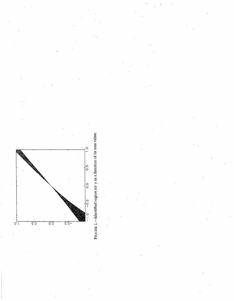
Imbens/Wooldridge, Lecture Notes 9, Summer ’07 11
bidder whether that bidder is still participating in the auction. (Milgrom and Weber (1982)
assume that each bidder continuously confirms their participation by holding down a button
while prices rise continuously.) In that case one would be able to infer for each bidder their
valuation, and thus directly estimate the value distribution.
This is not what is typically observed. Instead of prices rising continuously, there are
jumps in the bids, and for each bidder we do not know at any point in time whether they are
still participating unless they subsequently make a higher bid. HT study identification in
this, more realistic, setting. They assume that no bidder ever bids more than their valuation,
and that no bidder will walk away and let another bidder win the auction if the winning
bid is lower than their own valuation. Under those two assumptions, HT show that one can
derive bounds on the value distribution.
One set of bounds they propose is as follows. Let the highest bid for participant i in
auction t be bit. The number of participants in auction t is nt. Ignoring any covariates,
let the distribution of the value for individual i, νit, be Fν(v). This distribution function is
the same for all auctions. Let Fb(b) = Pr(bit ≤ b) be the distribution function of the bids
(ignoring variation in the number of bidders by auction). This distribution can be estimated
because the bids are observed. The winning bid in auction t is Bt = maxi=1,...,nt bit. First
HT derive an upper bound on the distribution function Fν(v). Because no bidder ever bids
more than their value, it follows that bit ≤ νit. Hence, without additional assumptions,
Fν(v) ≤ Fb(v), for all v.
For a lower bound on the distribution function one can use the fact that the second
highest of the values among the n participants in auction t must be less than or equal to the
winning bid. This follows from the assumption that no participant will let someone else win
with a bid below their valuation. Let Fν,m:n(v) denote the mth order statistic in a random
sample of size n from the value distribution, and let FB,n:n(b) denote the distribution of the
Imbens/Wooldridge, Lecture Notes 9, Summer ’07 12
winning bid in auctions with n participants. Then
FB,n:n(v) ≤ Fν,n−1:n(v).
The distribution of the any order statistic is monotonically related to the distribution of the
parent distribution, and so a lower bound on Fν,n−1:n(v) implies a lower bound on Fν(v).
HT derive tighter bounds based on the information in other bids and the inequalities
arising from the order statistics, but the above discussion illustrates the point that outside
of the Milgrom-Weber button auction model one can still derive bounds on the value dis-
tribution in an English auction even if one cannot point-identify the value distribution. If
in fact the highest bid for each individual was equal to their value (other than for the win-
ner for whom the bid is equal to the second highest value), the bounds would collaps and
point-identification would be obtained.
2.6 Entry Models and Inequality Conditions
Recently a number of papers has studied entry models in settings with multiple equilibria.
In such settings traditionally researchers have added ad hoc equilbrium selection mechanisms.
In the recent literature a key feature is the avoidance of such assumptions, as these are often
difficult to justify on theoretical grounds. Instead the focus is on what can be learned in the
absence of such assumptions. In this section I will discuss some examples from this literature.
An important feature of these models is that they often lead to inequality restrictions, where
the parameters of interest θ satisfy
E[ψ(Z, θ)] ≥ 0,
for known ψ(z, θ). This relates closely to the standard (Hansen, 1983) generalized method of
moments (GMM) set up where the functions ψ(Z, θ) would have expectation equal to zero at
the true values of the parameters. We refer to this as the generalized inequality restrictions
(GIR) form. These papers include Pakes, Porter, Ho, and Ishii (2006), Cilberto and Tamer
(2004, CM from hereon), Andrews, Berry and Jia (2004). Here I will discuss a simplified
Imbens/Wooldridge, Lecture Notes 9, Summer ’07 13
version of the CM model. Suppose two firms, A and B, contest a set of markets. In market
m, m = 1, . . . ,M , the profits for firms A and B are
πAm = αA + δA · dBm + εAm, and πBm = αB + δB · dAm + εBm.
where dFm = 1 if firm F is present in market m, for F ∈ A,B, and zero otherwise. The
more realistic model CM consider also includes observed market and firm characteristics.
Firms enter market m if their profits in that market are positive. Firms observe all compo-
nents of profits, including those that are unobserved to the econometrician, (εAm, εBm), and
so their decisions satisfy:
dAm = 1πAm ≥ 0, dBm = 1πBm ≥ 0. (1)
(Pakes, Porter, Ho, and Ishii allow for incomplete information where expected profits are
at least as high for the action taken as for actions not taken, given some information set.)
The unobserved (to the econometrician) components of profits, εFm, are independent accross
markets and firms. For ease of exposition we assume here that they have a normal N (0, 1)
distribution. (Note that we only observe indicators of the sign of profits, so the scale of
the unobserved components is not relevant for predictions.) The econometrician observes in
each market only the pair of indicators dA and dB . We focus on the case where the effect of
entry of the other firm on a firm’s profits, captured by the parameters δA and δB is negative,
which is the case of most economic interest.
An important feature of this model is that given the parameters θ = (αA, δA, αB, δB), for
a given set of (εAm, εBm) there is not necessarily a unique solution (dAm, dBm). For pairs of
values (εAm, εBm) such that
−αA < εA ≤ −αA − δA, −αB < εB ≤ −αB − δB,
both (dA, dB) = (0, 1) and (dA, dB) = (1, 0) satisfy the profit maximization condition (1).
In the terminology of this literature, the model is not complete. It does not specify the
Imbens/Wooldridge, Lecture Notes 9, Summer ’07 14
outcomes given the inputs. Figure 1, adapted from CM, shows the different regions in the
(εAm, εBm) space.
The implication of this is that the probability of the outcome (dAm, dBm) = (0, 1) cannot
be written as a function of the parameters of the model, θ = (αA, δA, αB, δB), even given
distributional assumptions on (εAm, εBm). Instead the model implies a lower and upper
bound on this probability:
HL,01(θ) ≤ Pr ((dAm, dBm) = (0, 1)) ≤ HU,01(θ).
Inspecting Figure 1 shows that
HL,01(θ) = Pr(εAm < −αA,−αB < εBm)
+Pr(−αA ≤ εAm < −αA − δA,−αB − δB < εBm),
and
HU,01(θ) = Pr(εAm < −αA, αB < εBm)
+Pr(−αA ≤ εAm < −αA − δA,−αB − δB < εBm),
+Pr(−αA ≤ εAm < −αA − δA,−αB < εBm < −αB − δB),
Similar expressions can be derived for the probability Pr ((dAm, dBm) = (1, 0)). Thus in
general we can write the information about the parameters in large samples as
HL,00(θ)HL,01(θ)HL,10(θ)HL,11(θ)
≤
Pr ((dAm, dBm) = (0, 0))Pr ((dAm, dBm) = (0, 1))Pr ((dAm, dBm) = (1, 0))Pr ((dAm, dBm) = (1, 1))
≤
HU,00(θ)HU,01(θ)HU,11(θ)HU,11(θ)
.
(For (dA, dB) = (0, 0) or (dA, dB) = (1, 1) the lower and upper bound coincide, but for ease
of exposition we treat all four configurations symmetrically.) The HL,ij(θ) and HU,ij(θ) are
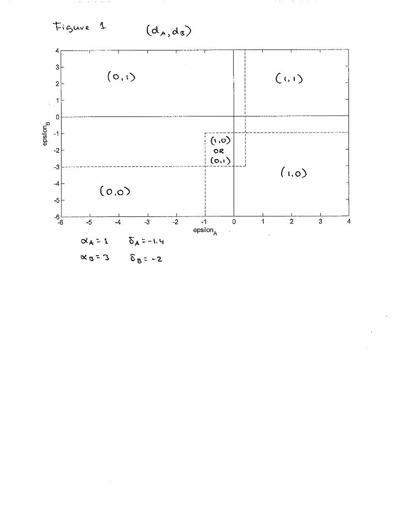
Imbens/Wooldridge, Lecture Notes 9, Summer ’07 15
known functions of θ. The data allow us to estimate the foru probabilities, which contain
only three separate pieces of information because the probabilities add up to one. Given
these probabilities, the identified set is the set of all θ that satisfy all eight inequalities. In
the simple model above, there are four parameters. Even in the case with the lower and
upper bounds for the probabilities coinciding, these would in general not be identified.
We can write this in the GIR form by defining
ψ(dA, dB |αA, αB, δA, δB) =
HU,00(θ) − (1 − dA) · (1 − dB)(1 − dA) · (1 − dB) −HL,00(θ)HU,01(θ) − (1 − dA) · dB
(1 − dA) · dB −HL,01(θ)HU,10(θ) − dA · (1 − dB)dA · (1 − dB) −HL,10(θ)HU,11(θ) − dA · dB
dA · dB −HL,11(θ)
,
so that the model implies that at the true values of the parameters
E [ψ(dA, dB |αA, αB, δA, δB)] ≥ 0.
3. Estimation
Chernozhukov, Hong, and Tamer (2007, CHT) consider, among other things, the case
with moment inequality conditions,
E[ψ(Z, θ)] ≥ 0,
where ψ(z, θ) is a known vector of functions, of dimension M , and the unknown parameter
θ is of dimension K. Let Θ be the parameter space, a subset of RK .
Define for a vector x the vector (x)+ to be the component-wise non-negative part, and
(x)− to be the component-wise non-positive part, so that for all x, x = (x)− + (x)+. For a
givenM×M non-negative definite weight matrix W , CHT consider the population objective
function
Q(θ) = E[ψ(Z, θ)]′−WE[ψ(Z, θ)]−.
Imbens/Wooldridge, Lecture Notes 9, Summer ’07 16
For all θ in the identified set, denoted by ΘI ⊂ Θ, we have Q(θ) = 0.
The sample equivalent to this population objective function is
QN(θ) =
(
1
N
N∑
i=1
ψ(Zi, θ)
)′
−
W
(
1
N
N∑
i=1
ψ(Zi, θ)
)
−
.
We cannot simply estimate the identified set as
ΘI = θ ∈ Θ |QN (θ) = 0 ,
The reason is that even for θ in the identified setQN (θ) may be positive with high probability.
A simple way to see that is to consider the standard GMM case with equalities and over-
identification. If E[ψ(Z, θ)] = 0, the objective function will not be zero in finite samples in
the case with over-identification. As a result, ΘI can be empty when ΘI is not, even in large
samples.
This is the reason CHT estimate the set ΘI as
ΘI = θ ∈ Θ |QN (θ) ≤ aN ,
where aN → 0 at the appropriate rate. In most regular problems aN = c/N , leading to an
estimator ΘI that is consistent for ΘI , by which we mean that the two sets get close to each
other, in the Hausdorf sense that
supθ∈ΘI
infθ′∈ΘI
d(θ, θ′) −→ 0, and supθ′∈ΘI
infθ∈ΘI
d(θ, θ′) −→ 0,
where d(θ, θ′) = ((θ − θ)′(θ − θ′))1/2.
3. Inference: General Issues
There is a rapidly growing literature concerned with developing methods for inference in
partially identified models, including Beresteanu and Molinari (2006), Chernozhukov, Hong,
and Tamer (2007), Imbens and Manski (2004), Rosen (2006), and Romano and Shaikh
Imbens/Wooldridge, Lecture Notes 9, Summer ’07 17
(2007ab). In many cases the partially identified set itself is difficult to characterize. In the
scalar case this can be much simpler. There it often is an interval, [θLB, θUB]. There are by
now a number of proposals for constructing confidence sets. They differ in implementation
as well as in their goals. One issue is whether one wants a confidence set that includes
each element of the identified set with fixed probability, or the entire identified set with that
probability. Formally, the first question looks for a confidence set CIθα that satisfies
infθ∈[θLB,θUB]
Pr(
θ ∈ CIθα
)
≥ α.
In the second case we look for a set CI[θLB,θUB]
α such that
Pr(
[θLB, θUB] ⊂ CIθα)
≥ α.
The second requirement is stronger than the first, and so generally CIθα ⊂ CI[θLB,θUB]
α . Here
we follow Imbens and Manski (2004) and Romano and Shaikh (2007a) who focus on the
first case. This seems more in line with teh traditional view of confidence interval in that
they should cover the true value of the parameter with fixed probability. It is not clear why
the fact that the object of interest is not point-identified should change the definition of a
confidence interval. CHT and Romano and Shaikh (2007b) focus on the second case.
Next we discuss two specific examples to illustrate some of the issues that can arise, in
particular the uniformity of confidence intervals.
3.1 Inference: A Missing Data Problem
Here we continue the missing data example from Section 2.1. We have a random sample
of (Wi,Wi · Yi), for i = 1, . . . , N . Yi is known to lie in the interval [0, 1], interest is in
θ = E[Y ], and the parameter space is Θ = [0, 1]. Define µ1 = E[Y |W = 1], λ = E[Y |W = 0],
σ2 = V(Y |W = 1), and p = E[W ]. For ease of exposition we assume p is known. The
identified set is
ΘI = [p · µ1, p · µ1 + (1 − p)].
Imbens/Wooldridge, Lecture Notes 9, Summer ’07 18
Imbens and Manski (2004) discuss confidence intervals for this case. The key feature of this
problem, and similar ones, is that the lower and upper bounds are well-behaved functionals
of the joint distribution of the data that can be estimated at the standard parametric√N
rate with an asymptotic normal distribution. In this specific example the lower and upper
bound are both functions of a single unknown parameter, the conditional mean µ1. The first
step is a 95% confidence interval for µ1. Let N1 =∑
i Wi and Y 1 =∑
iWi · Yi/N1. The
standard confidence interval is
CIµ1
α =[
Y − 1.96 · σ/√N1, Y + 1.96 · σ/
√N1
]
.
Consider the confidence interval for the lower and upper bound:
CIp·µ1
α =[
p ·(
Y − 1.96 · σ/√N 1
)
, p ·(
Y + 1.96 · σ/√N1
)]
,
and
CIp·µ1+(1−p)
α =[
p ·(
Y − 1.96 · σ/√N1
)
+ (1 − p), p ·(
Y + 1.96 · σ/√N1
)
+ 1 − p]
.
A simple and valid confidence interval can be based on the lower confidence bound on the
lower bound and the upper confidence bound on the upper bound:
CIθα =
[
p ·(
Y − 1.96 · σ/√N1
)
, p ·(
Y + 1.96 · σ/√N 1
)
+ 1 − p]
.
This is generally conservative. For each θ in the interior of ΘI, the asymptotic coverage rate
is 1. For θ ∈ θLB, θUB, the coverage rate is α + (1 − α)/2.
The interval can be modified to give asymptotic coverage equal to α by changing the
quantiles used in the confidence interval construction, essentially using one-sided critical
values,
CIθα =
[
p ·(
Y − 1.645 · σ/√N 1
)
, p ·(
Y + 1.645 · σ/√N1
)
+ 1 − p]
.
Imbens/Wooldridge, Lecture Notes 9, Summer ’07 19
This has the problem that if p = 0 (when θ is point-identified), the coverage is only α−(1−α).
In fact, for values of p close to zero, the confidence interval would be shorter than the
confidence interval in the point-identified case. Imbens and Manski (2004) suggest modifying
the confidence interval to
CIθα =
[
p ·(
Y − CN · σ/√N1
)
, p ·(
Y + CN · σ/√N1
)
+ 1 − p]
,
where the critical value CN satisfies
Φ
(
CN +√N · 1 − p
σ/√p
)
− Φ(−CN ) = α.
and CN = 1.96 if p = 0. This confidence interval has asymptotic coverage 0.95, uniformly
over p.
3.2. Inference: Multiple Inequalities
Here we look at inference in the Genereralized Inequality (GIR) setting. The example is
a simplified version of the moment inequality type of problems discussed in CHT, Romano
and Shaikh (2007ab), Pakes, Porter, Ho, and Ishii (2006), and Andrews and Guggenberger
(2007). Suppose we have two moment inequalities,
E[X] ≥ θ, and E[Y ] ≥ θ.
The parameter space is Θ = [0,∞). Let µX = E[X], and µY = E[Y ]. We have a random
sample of size N of the pairs (X, Y ). The identified set is
ΘI = [0,min(µX , µY )].
The key difference with the previous example is that the upper bound is no longer a
smooth, well-behaved functional of the joint distribution. In the simple two-inequality ex-
ample, if µX is close to µY , the distribution of the estimator for the upper bound is not well
approximated by a normal distribution. Suppose we estimate the means of X and Y by
Imbens/Wooldridge, Lecture Notes 9, Summer ’07 20
X, and Y , and that the variances of X and Y are known to be equal to σ2. A naive 95%
confidence interval would be
Cθα = [0,min(X, Y ) + 1.645 · σ/N ].
This confidence interval essentially ignores the moment inequality that is not binding in the
sample. It has asymptotic 95% coverage for all values of µX , µY , as long as min(µX , µY ) > 0,
and µX 6= µY . The first condition (min(µX , µY ) > 0) is the same as the condition in the
Imbens-Manski example. It can be dealt with in the same way by adjusting the critical value
slightly based on an initial estimate of the width of the identified set.
The second condition raises a different uniformity concern. The naive confidence interval
essentially assumes that the researcher knows which moment conditions are binding. This is
true in large samples, unless there is a tie. However, in finite samples ignoring uncertainty
regarding the set of binding moment inequalities may lead to a poor approximation, especially
if there are many inequalities. One possibility is to construct conservative confidence intervals
(e.g., Pakes, Porter, Ho, and Ishii, 2007). However, such intervals can be unnecessarily
conservative if there are moment inequalities that are far from binding.
One would like construct confidence intervals that asymptotically ignore irrelevant in-
equalities, and at the same time are valid uniformly over the parameter space. Bootstrap-
ping is unlikely to work in this setting. One way of obtaining confidence intervals that are
uniformly valid is based on subsampling. See Romano and Shaikh (2007a), and Andrews
and Guggenberger (2007). Little is known about finite sample properties in realistic settings.
Imbens/Wooldridge, Lecture Notes 9, Summer ’07 21
References
Andrews, D., S. Berry, and P. Jia (2004), “Confidence Regions for Parameters
in Discrete Games with Multiple Equilibria, with an Application to Discount Chain Store
Location,”unpublished manuscript, Department of Economics, Yale University.
Andrews, D., and P. Guggenberger (2004), “The Limit of Finite Sample Size
and a Problem with Subsampling,”unpublished manuscript, Department of Economics, Yale
University.
Aradillas-Lopez, A., and E. Tamer (2007), “The Identification Power of Equilib-
rium in Games,”unpublished manuscript, Department of Economics, Princeton University.
Balke, A., and J. Pearl, (1997), “Bounds on Treatment Effects from Studies with
Imperfect Compliance,”Journal of the American Statistical Association, 92: 1172-1176.
Beresteanu, A., and F. Molinari, (2006), “Asymptotic Properties for a Class of
Partially Identified Models,”Unpublished Manuscript, Department of Economics, Cornell
University.
Blundell, R., M. Browning, and I. Crawford, (2007), “Best Nonparametric
Bounds on Demand Responses,”Cemmap working paper CWP12/05, Department of Eco-
nomics, University College London.
Blundell, R., A. Gosling, H. Ichimura, and C. Meghir, (2007), “Changes in
the Distribution of Male and Female Wages Accounting for Employment Composition Using
Bounds,”Econometrica, 75(2): 323-363.
Chernozhukov, V., H. Hong, and E. Tamer (2007), “Estimation and Confidence
Regions for Parameter Sets in Econometric Models,”forthcoming, Econometrica.
Ciliberto, F., and E. Tamer (2004), “Market Structure and Multiple Equilibria in
Airline Markets,”Unpublished Manuscript.
Haile, P., and E. Tamer (2003), “Inference with an Incomplete Model of English
Auctions,”Journal of Political Economy, Vol 111(1), 1-51.
Heckman, J., (1978), “Dummy Endogenous Variables in a Simultaneous Equations
Imbens/Wooldridge, Lecture Notes 9, Summer ’07 22
System”, Econometrica, Vol. 46, 931–61.
Heckman, J. J. (1990), ”Varieties of Selection Bias,” American Economic Review 80,
313-318.
Honore, B., and E. Tamer (2006), “Bounds on Parameters in Dynamic Discrete
Choice Models,”Econometrica, 74(3): 611-629.
Hotz, J., C. Mullin, and S. Sanders, (1997), “Boudning Causal Effects Using Data
from a Contaminated Natural Experiment: Analysing the Effects of Teenage Childbearing,”
Review of Economic Studies, 64(4), 575-603.
Imbens, G., and C. Manski (2004), “Confidence Intervals for Partially Identified
Parameters,”Econometrica, 74(6): 1845-1857.
Manski, C., (1990), “Nonparametric Bounds on Treatment Effects,”American Economic
Review Papers and Proceedings, 80, 319-323.
Manski, C. (1995), Identification Problems in the Social Sciences, Cambridge, Harvard
University Press.
Manski, C. (2003), Partial Identification of Probability Distributions, New York: Springer-
Verlag.
Manski, C., and J. Pepper, (2000), “Monotone Instrumental Variables: With an
Application to the Returns to Schooling,”Econometrica, 68(): 997-1010.
Manski, C., G. Sandefur, S. McLanahan, and D. Powers (1992), “Alternative
Estimates of the Effect of Family Structure During Adolescence on High School,”Journal of
the American Statistical Association, 87(417):25-37.
Milgrom, P, and R. Weber (1982), “A Theory of Auctions and Competitive Bid-
ding,”Econometrica, 50(3): 1089-1122.
Pakes, A., J. Porter, K. Ho, and J. Ishii (2006), “Moment Inequalities and Their
Application,”Unpublished Manuscript.
Robins, J., (1989), “The Analysis of Randomized and Non-randomized AIDS Trials Us-
ing a New Approach to Causal Inference in Longitudinal Studies,”in Health Service Research
Imbens/Wooldridge, Lecture Notes 9, Summer ’07 23
Methodology: A Focus on AIDS, (Sechrest, Freeman, and Mulley eds), US Public Health
Service, 113-159.
Romano, J., and A. Shaikh (2006a), “Inference for Partially Identified Parame-
ters,”Unpublished Manuscript, Stanford University.
Romano, J., and A. Shaikh (2006b), “Inference for Partially Identified Sets,”Unpublished
Manuscript, Stanford University.
Rosen, A., (2005), “Confidence Sets for Partially Identified Parameters that Satisfy a Fi-
nite Number of Moment Inequalities,” Unpublished Manuscript, Department of Economics,
University College London.
Wooldridge, J (2002), “Simple Solutions to the Initial Conditions Problem in Dy-
namic, Nonlinear Panel Data Models with Unobserved Heterogeneity,”Journal of Applied
Econometrics, 20, 39-54.
Imbens/Wooldridge, Lecture Notes 10, Summer ’07
What’s New in Econometrics? NBER, Summer 2007Lecture 10, Tuesday, July 31st, 4.30-5.30 pm
Difference-in-Differences EstimationThese notes provide an overview of standard difference-in-differences methods that have
been used to study numerous policy questions. We consider some recent advances in Hansen(2007a,b) on issues of inference, focusing on what can be learned with various group/timeperiod dimensions and serial independence in group-level shocks. Both the repeated crosssections and panel data cases are considered. We discuss recent work by Athey and Imbens(2006) on nonparametric approaches to difference-in-differences, and Abadie, Diamond, andHainmueller (2007) on constructing synthetic control groups.1. Review of the Basic Methodology
Since the work by Ashenfelter and Card (1985), the use of difference-in-differencesmethods has become very widespread. The simplest set up is one where outcomes are observedfor two groups for two time periods. One of the groups is exposed to a treatment in the secondperiod but not in the first period. The second group is not exposed to the treatment duringeither period. In the case where the same units within a group are observed in each time period,the average gain in the second (control) group is substracted from the average gain in the first(treatment) group. This removes biases in second period comparisons between the treatmentand control group that could be the result from permanent differences between those groups, aswell as biases from comparisons over time in the treatment group that could be the result oftrends. We will treat the panel data case in Section 4.
With repeated cross sections, we can write the model for a generic member of any ofgroups as
y 0 1dB 0d2 1d2 dB u (1.1)
where y is the outcome of interest, d2 is a dummy variable for the second time period. Thedummy variable dB captures possible differences between the treatment and control groupsprior to the policy change. The time period dummy, d2, captures aggregate factors that wouldcause changes in y even in the absense of a policy change. The coefficient of interest, 1,multiplies the interaction term, d2 dB, which is the same as a dummy variable equal to onefor those observations in the treatment group in the second period. Thedifference-in-differences estimate is
1 yB,2 − yB,1 − yA,2 − yA,1. (1.2)
1
Imbens/Wooldridge, Lecture Notes 10, Summer ’07
Inference based on even moderate sample sizes in each of the four groups is straightforward,and is easily made robust to different group/time period variances in the regression framework.
In some cases a more convincing analysis of a policy change is available by furtherrefining the definition of treatment and control groups. For example, suppose a stateimplements a change in health care policy aimed at the elderly, say people 65 and older, andthe response variable, y, is a health outcome. One possibility is to use data only on people inthe state with the policy change, both before and after the change, with the control group beingpeople under 65 and the treatment group being people 65 and older. The potential problemwith this DD analysis is that other factors unrelated to the state’s new policy might affect thehealth of the elderly relative to the younger population, for example, changes in health careemphasis at the federal level. A different DD analysis would be to use another state as thecontrol group and use the elderly from the non-policy state as the control group. Here, theproblem is that changes in the health of the elderly might be systematically different acrossstates due to, say, income and wealth differences, rather than the policy change.
A more robust analysis than either of the DD analyses described above can be obtained byusing both a different state and a control group within the treatment state. If we again label thetwo time periods as one and two, let B represent the state implementing the policy, and let Edenote the group of elderly, then an expanded verson of (1.1) is
y 0 1dB 2dE 3dB dE 0d2 1d2 dB 2d2 dE 3d2 dB dE u (1.3)
The coefficient of interest is now 3, the coefficient on the triple interaction term, d2 dB dE.The OLS estimate 3 can be expressed as follows:
3 yB,E,2 − yB,E,1 − yA,E,2 − yA,E,1 − yB,N,2 − yB,N,1 (1.4)
where the A subscript means the state not implementing the policy and the N subscriptrepresents the non-elderly. For obvious reasons, the estimator in (1.4) is called thedifference-in-difference-in-differences (DDD) estimate. [The population analog of (1.4) iseasily established from (1.3) by finding the expected values of the six groups appearing in(1.4).] If we drop either the middle term or the last term, we obtain one of the DD estimatesdescribed in the previous paragraph. The DDD estimate starts with the time change in averagesfor the elderly in the treatment state and then nets out the change in means for elderly in thecontrol state and the change in means for the non-elderly in the treatment state. The hope isthat this controls for two kinds of potentially confounding trends: changes in health status of
2

Imbens/Wooldridge, Lecture Notes 10, Summer ’07
elderly across states (that would have nothing to do with the policy) and changes in healthstatus of all people living in the policy-change state (possibly due to other state policies thataffect everyone’s health, or state-specific changes in the economy that affect everyone’shealth). When implemented as a regression, a standard error for 3 is easily obtained, includinga heteroskedasticity-robust standard error. As in the DD case, it is straightforward to addadditional covariates to (1.3) and inference robust to heteroskedasticity.2. How Should We View Uncertainty in DD Settings?
The standard approach just described assumes that all uncertainty in inference entersthrough sampling error in estimating the means of each group/time period combination. Thisapproach has a long history in statistics, as it is equivalent to analysis of variance. Recently,different approaches have been suggest that focus on different kinds of uncertainty – perhapsin addition to sampling error in estimating means. Recent work by Bertrand, Duflo, andMullainathan (2004), Donald and Lang (2007), Hansen (2007a,b), and Abadie, Diamond, andHainmueller (2007) argues for additional sources of uncertainty. In fact, in most cases theadditional uncertainty is assumed to swamp the sampling error in estimating group/time periodmeans. We already discussed the DL approach in the cluster sample notes, although we did notexplicitly introduce a time dimension. One way to view the uncertainty introduced in the DLframework – and a perspective explicitly taken by ADH – is that our analysis should betterreflect the uncertainty in the quality of the control groups.
Before we turn to a general setting, it is useful to ask whether introducing more thansampling error into DD analyses is necessary, or desirable. As we discussed in the clustersample notes, the DL approach does not allow inference in the basic comparison-of-mean casefor two groups. While the DL estimate is the usual difference in means, the error variance ofthe cluster effect cannot be estimated, and the t distribution is degenerate. It is also the casethat the DL approach cannot be applied to the standard DD or DDD cases covered in Section 1.We either have four different means to estimate or six, and the DL regression in these casesproduces a perfect fit with no residual variance. Should we conclude nothing can be learned insuch settings?
Consider the example from Meyer, Viscusi, and Durbin (1995) on estimating the effects ofbenefit generosity on length of time a worker spends on workers’ compensation. MVD have abefore and after period, where the policy change was to raise the cap on covered earnings. Thetreatment group is high earners, and the control group is low earners – who should not have
3
Imbens/Wooldridge, Lecture Notes 10, Summer ’07
been affected by the change in the cap. Using the state of Kentucky and a total sample size of5,626, MVD find the DD estimate of the policy change is about 19.2% (longer time onworkers’ compensation). The t statistic is about 2.76, and the estimate changes little whensome controls are added. MVD also use a data set for Michigan. Using the same DD approach,they estimate an almost identical effect: 19.1%. But, with “only” 1,524 observations, the tstatistic is 1.22. It seems that, in this example, there is plenty of uncertainty in estimation, andone cannot obtain a tight estimate without a fairly large sample size. It is unclear what we gainby concluding that, because we are just identifying the parameters, we cannot performinference in such cases. In this example, it is hard to argue that the uncertainty associated withchoosing low earners within the same state and time period as the control group somehowswamps the sampling error in the sample means.3. General Settings for DD Analysis: Multiple Groups and TimePeriods
The DD and DDD methodologies can be applied to more than two time periods. In the firstcase, a full set of time-period dummies is added to (1.1), and a policy dummy replaces d2 dB;the policy dummy is simply defined to be unity for groups and time periods subject to thepolicy. This imposes the restriction that the policy has the same effect in every year, andassumption that is easily relaxed. In a DDD analysis, a full set of dummies is included for eachof the two kinds of groups and all time periods, as well as all pairwise interactions. Then, apolicy dummy (or sometimes a continuous policy variable) measures the effect of the policy.See Gruber (1994) for an application to mandated maternity benefits.
With many time periods and groups, a general framework considered by BDM (2004) andHansen (2007b) is useful. The equation at the individual level is
yigt t g xgt zigtgt vgt uigt, i 1, . . . ,Mgt, (3.1)
where i indexes individual, g indexes group, and t indexes time. This model has a full set oftime effects, t, a full set of group effects, g, group/time period covariates, xgt (these are the
policy variables), individual-specific covariates, zigt, unobserved group/time effects, vgt, and
individual-specific errors, uigt. We are interested in estimating . Equation (3.1) is an example
of a multilevel model.One way to write (3.1) that is useful is
yigt gt zigtgt uigt, i 1, . . . ,Mgt, (3.2 )
4
Imbens/Wooldridge, Lecture Notes 10, Summer ’07
which shows a model at the individual level where both the intercepts and slopes are allowedto differ across all g, t pairs. Then, we think of gt as
gt t g xgt vgt. (3.3)
Equation (3.3) is very useful, as we can think of it as a regression model at the group/timeperiod level.
As discussed by BDM, a common way to estimate and perform inference in (3.1) is toignore vgt, in which case the observations at the individual level are treated as independent.
When vgt is present, the resulting inference can be very misleading. BDM and Hansen (2007b)
allow serial correlation in vgt : t 1,2, . . . ,T and assume independence across groups, g.
A simple way to proceed is to view (3.3) as ultimately of interest. We observe xgt, t is
handled with year dummies,and g just represents group dummies. The problem, then, is that
we do not observe gt. But we can use the individual-level data to estimate the gt, provided
the group/time period sizes, Mgt, are reasonably large. With random sampling within each
g, t, the natural estimate of gt is obtained from OLS on (3.2) for each g, t pair, assuming
that Ezigt′ uigt 0. (In most DD applications, this assumption almost holds by definition, as
the individual-specific controls are included to improve estimation of gt.) If a particular model
of heteroskedasticity suggests itself, and Euit|zigt 0 is assumed, then a weighted least
squares procedure can be used. Sometimes one wishes to impose some homogeneity in theslopes – say, gt g or even gt – in which case pooling can be used to impose such
restrictions. In any case, we proceed as if the Mgt are large enough to ignore the estimation
error in the gt; instead, the uncertainty comes through vgt in (3.3). Hansen (2007b) considers
adjustments to inference that accounts for sampling error in the gt, but the methods are more
complicated. The minimum distance approach we discussed in the cluster sampling notes,applied in the current context, effectively drops vgt from (3.3) and views gt t g xgt
as a set of deterministic restrictions to be imposed on gt. Inference using the efficient
minimum distance estimator uses only sampling variation in the gt, which will be independent
across all g, t if they are separately estimated, or which will be correlated if pooled methodsare used.
Because we are ignoring the estimation error in gt, we proceed simply by analyzing the
panel data equation
gt t g xgt vgt, t 1, . . . ,T,g 1, . . . ,G, (3.4)
5
Imbens/Wooldridge, Lecture Notes 10, Summer ’07
where we keep the error as vgt because we are treating gt and gt interchangeably. If we
assume that We can apply the BDM findings and Hansen (2007a) results directly to thisequation. Namely, if we estimate (3.4) by OLS – which means full year and group effects,along with xgt – then the OLS estimator has satisfying properties as G and T both increase,
provided vgt : t 1,2, . . . ,T is a weakly dependent (mixing) time series for all g. The
simulations in BDM and Hansen (2007a) indicate that cluster-robust inference, where eachcluster is a set of time periods, work reasonably well when vgt follows a stable AR(1) model
and G is moderately large.Hansen (2007b), noting that the OLS estimator (the fixed effects estimator) applied to (3.4)
is inefficient when vgt is serially uncorrelated (and possibly heteroskedastic), proposes feasible
GLS. As is well known, if T is not large, estimating parameters for the variance matrixg Varvg, where vg is the T 1error vector for each g, is difficult when group effects
have been removed. In other words, using the FE residuals, vgt, to estimate g can result in
severe bias for small T. Solon (1984) highlighted this problem for the homoskedastic AR(1)model. Of course, the bias disappears as T → , and regression packages such as Stata, thathave a built-in command to do fixed effects with AR(1) errors, use the usual AR(1) coefficient, obtained from
vgt on vg,t−1, t 2, . . . ,T,g 1, . . . ,G. (3.5)
As discussed in Wooldridge (2003) and Hansen (2007b), one way to account for the bias in is to still use a fully robust variance matrix estimator. But Hansen’s simulations show that thisapproach is quite inefficient relative to his suggestion, which is to bias-adjust the estimator and then use the bias-adjusted estimator in feasible GLS. (In fact, Hansen covers the generalARp model.) Hansen derives many attractive theoretical properties of his the estimator.Aniterative bias-adjusted procedure has the same asymptotic distribution as in the case shouldwork well: G and T both tending to infinity. Most importantly for the application to DDproblems, the feasible GLS estimator based on the iterative procedure has the same asymptoticdistribution as the GLS etsimator when G → and T is fixed. When G and T are both large,there is no need to iterated to achieve efficiency.
Hansen further shows that, even when G and T are both large, so that the unadjusted ARcoefficients also deliver asymptotic efficiency, the bias-adusted estimates deliver higher-orderimprovements in the asymptotic distribution. One limitation of Hansen’s results is that theyassume xgt : t 1, . . . ,T are strictly exogenous. We know that if we just use OLS – that is,
6
Imbens/Wooldridge, Lecture Notes 10, Summer ’07
the usual fixed effects estimate – strict exogeneity is not required for consistency as T → .GLS, in exploiting correlations across different time periods, tends to exacerbate bias thatresults from a lack of strict exogeneity. In policy analysis cases, this is a concern if the policiescan switch on and off over time, because one must decide whether the decision to implementor remove a program is related to past outcomes on the response.
With large G and small T, one can estimate an unstricted variance matrix g and proceed
with GLS – this is the approach suggested by Kiefer (1980) and studied more recently byHausman and Kuersteiner (2003). It is equivalent to dropping a time period in thetime-demeaned equation and proceeding with full GLS (and this avoids the degeneracy in thevariance matrix of the time-demeaned errors). Hausman and Kuersteiner show that the Kieferapproach works pretty well when G 50 and T 10, although substantial size distortionsexist for G 50 and T 20.
Especially if the Mgt are not especially large, we might worry about ignoring the estimation
error in the gt. One simple way to avoid ignoring the estimation error in gt is to aggregate
equation (3.1) over individuals, giving
ygt t g xgt zgt vgt ūgt, t 1, . . ,T,g 1, . . . ,G. (3.6)
Of course, this equation can be estimated by fixed effects, too, and fully robust inference isavailable using Hansen (2007a) because the composite error, rgt ≡ vgt ūgt, is weakly
dependent. Fixed Effects GLS using an unrestricted variance matrix can be used with large Gand small T. The complication with using specific time series model for the error is thepresence of ūgt. With different Mgt, Varūgt is almost certainly heteroskedastic (and might be
with the same Mgt, of course). So, even if we specify, say, an AR(1) model vgt vg,t−1 egt,
the variance matrix of rg is more complicated. One possibility is to just assume the composite
error, rgt, follows a simple model, implement Hansen’s methods, but then use fully robust
inference.The Donald and Land (2007) approach applies in the current setting by using finite sample
analysis applied to the pooled regression (3.4). However, DL assume that the errors vgt are
uncorrelated across time, and so, even though for small G and T it uses smalldegrees-of-freedom in a t distribution, it does not account for uncertainty due to serialcorrelation in vgt : t 1, . . . ,T.
4. Individual-Level Panel DataIndividual-level panel data is a powerful tool for estimating policy effects. In the simplest
7
Imbens/Wooldridge, Lecture Notes 10, Summer ’07
case we have two time periods and a binary program indicator, wit, which is unity if unit iparticipates in the program at time t. A simple, effective model is
yit d2t wit ci uit, t 1,2, (4.1)
where d2t 1 if t 2 and zero otherwise, ci is an observed effect, and uit are the idiosyncraticerrors. The coefficient is the treatment effect. A simple estimation procedure is to firstdifference to remove ci :
yi2 − yi1 wi2 − wi1 ui2 − ui1 (4.2)
or
Δyi Δwi Δui. (4.3)
If EΔwiΔui 0, that is, the change in treatment status is uncorrelated with changes in theidiosyncratic errors, then OLS applied to (4.3) is consistent. The leading case is when wi1 0for all i, so that no units we exposed to the program in the initial time period. Then the OLSestimator is
Δytreat − Δycontrol, (4.4)
which is a difference-in-differences estimate except that we different the means of the sameunits over time.This same estimate can be derived without introducing heterogeneity by simplywriting the equation for yit with a full set of group-time effects. Also, (4.4) is not the sameestimate obtained from the regression yi2 on 1,yi1, wi2 – that is, using yi1 as a control in a crosssection regression. The estimates can be similar, but their consistency is based on differentassumptions.
More generally, with many time periods and arbitrary treatment patterns, we can use
yit t wit xit ci uit, t 1, . . . ,T, (4.5)
which accounts for aggregate time effects and allows for controls, xit. Estimation by FE or FDto remove ci is standard, provided the policy indicator, wit, is strictly exogenous: correlationbeween wit and uir for any t and r causes inconsistency in both estimators, although the FEestimator typically has smaller bias when we can assume conteporaneous exogeneity,Covwit,uit 0. Strict exogeneity can be violated if policy assignment changes in reaction topast outcomes on yit. In cases where wit 1 whenever wir 1 for r t, strict exogeneity isusually a reasonable assumption.
Equation (4.5) allows policy designation to depend on a level effect, ci, but wit might be
8
Imbens/Wooldridge, Lecture Notes 10, Summer ’07
correlated with unit-specific trends in the response, too. This suggests the “correlated randomtrend” model
yit ci git t wit xit uit, t 1, . . . ,T, (4.6)
where gi is the trend for unit i. A general analysis allows arbitrary corrrelation between ci,gi
and wit, which requires at least T ≥ 3. If we first difference, we get
Δyit gi t Δwit Δxit Δuit, t 2, . . . ,T, (4.7)
where t t − t−1 is a new set of time effects. We can estimate (4.7) by differencing again,or by using FE. The choice depends on the serial correlation properties in Δuit (assume strictexogeneity of treatment and covariates). If Δuit is roughly uncorrelated, FE is preferred. If theoriginal errors uit are essentially uncorrelated, applying FE to (4.6), in the general sense ofsweeping out the linear trends from the response, treatment, and covariates, is preferred. Fullyrobust inference using cluster-robust variance estimators is straightforward. Of course, onemight want to allow the effect of the policy to change over time, which is easy by interactingtime dummies with the policy indicator.
We can derive standard panel data approaches using the counterfactural framework fromthe treatment effects literature.For each i, t, let yit1 and yit0 denote the counterfactualoutcomes, and assume there are no covariates. One way to state the assumption ofunconfoundedness of treatment is that, for time-constant heterogeneity ci0 and ci1,
Eyit0|wi,ci0,ci1 Eyit0|ci0
Eyit1|wi,ci0,ci1 Eyit1|ci1, (4.8) (4.9)
where wi wi1, . . . ,wiT is the time sequence of all treatments. We saw this kind of strictexogeneity assumption conditional on latent variables several times before. It allows treatmentto be correlated with time-constant heterogeneity, but does not allow treatment in any timeperiod to be correlated with idiosyncratic changes in the counterfactuals. Next, assume that theexpected gain from treatment depends at most on time:
Eyit1|ci1 Eyit0|ci0 t, t 1, . . . ,T. (4.10)
Writing yit 1 − wityit0 wityi1, and using (4.8), (4.9), and (4.10) gives
Eyit|wi,ci0,ci1 Eyit0|ci0 witEyit1|ci1 − Eyit0|ci0
Eyit0|ci0 twit. (4.11)
If we now impose an additive structure on Eyit0|ci0, namely,
9
Imbens/Wooldridge, Lecture Notes 10, Summer ’07
Eyit0|ci0 t0 ci0, (4.12)
then we arrive at
Eyit|wi,ci0,ci1 t0 ci0 twit, (4.13)
an estimating equation that leads to well-known procedures. Because wit : t 1, . . . ,T isstrictly exogenous conditional on ci0, we can use fixed effects or first differencing, with a fullset of time period dummies. A standard analysis would use t , but, of course, we caneasily allow the effects of the policy to change over time.
Of course, we can add covariates xit to the conditioning sets and assume linearity, sayEyit0|xit,ci0 t0 xit0 ci0. If (4.8) becomes
Eyit0|wi,xi,ci0,ci1 Eyit0|xit,ci0, (4.14)
and similarly for (4.9), then the estimating equation simply adds xit0 to (4.13). More
interesting models are obtained by allowing the gain from treatment to depend onheterogeneity. Suppose we assume, in addition to the ignorability assumption in (4.14) (and theequivalent condition for yit1
Eyit1 − yit0|xit,ci0,ci1 t ai xit−t (4.15)
where ai is a function of ci0,ci1 normalized so that Eai 0 and t Exit. Equation
(4.15) allows the gain from treatment to depend on time, unobserved heterogeneity, andobserved covariates. Then
Eyit|wi,xi,ci0,ai t0 twit xit0
witxit−t ci0 aiwit.
(4.16)
This is a correlated random coefficient model because the coefficient on wit is t ai, whichhas expected value t. Generally, we want to allow wit to be correlated with ai and ci0. Withsmall T and large N, we do not try to estimate the ai (nor the ci0). But an extension of thewithin transformation effectively eliminates aiwit. Suppose we simplify a bit and assume t and drop all other covariates. Then, a regression that appears to suffer from anincidental parameters problem turns out to consistently estimate : Regress yit on yeardummies, dummies for each cross-sectional observation, and latter dummies interacted withwit. In other words, we estimate
ŷ it t0 ĉ i0 iwit. (4.17)
While i is usually a poor estimate of i ai, their average is a good estimator of :
10
Imbens/Wooldridge, Lecture Notes 10, Summer ’07
N−1∑i1
N
i. (4.18)
A standard error can be calculated using Wooldridge (2002, Section 11.2) or bootstrapping.We can apply the results from the linear panel data notes to determine when the usual FE
estimator – that is, the one that ignores aiwit – is consistent for . In addition to theunconfoundedness assumption, sufficient is
E i|wit E i , t 1, . . . ,T, (4.19)
where wit wit − wi. Essentially, the individual-specific treatment effect can be correlatedwith the average propensity to recieve treatment, wi, but not the deviations for any particulartime period.
Assumption (4.19) is not completely general, and we might want a simple way to tellwhether the treatment effect is heterogeneous across individuals. Here, we an exploitcorrelation between the i and treatment. Recalling that i ai, a useful assumption (thatneed not hold for obtaining a test) is
Eai|wi1, . . .wiT Eai|wi wi − wi, (4.20)
where other covariates have been suppressed. Then we can estimate the equation (withcovariates)
yit t0 wit xit0 witxit−xt
witwi − w ci0 eit
(4.21)
by standard fixed effects. Then, we use a simple t test on , robust to heteroskedasticity andserial correlation. If we reject, it does not mean the mean usual FE estimator is inconsistent,but it could be.5. Semiparametric and Nonparametric Approaches
Return to the setting with two groups and two time periods. Athey and Imbens (2006)generalize the standard DD model in several ways. Let the two time periods be t 0 and 1 andlabel the two groups g 0 and 1. Let Yi0 be the counterfactual outcome in the absense ofintervention and Yi1 the counterfactual outcome with intervention. AI assume that
Yi0 h0Ui,Ti, (5.1)
where Ti is the time period and
h0u, t strictly increasing in u for t 0,1 (5.2)
11
Imbens/Wooldridge, Lecture Notes 10, Summer ’07
The random variable Ui represents all unobservable characteristics of individual i. Equation(5.1) incorporates the idea that the outcome of an individual with Ui u will be the same in agiven time period, irrespective of group membership. The strict monotonicity assumption in(5.2) rules out discrete responses, but Athey and Imbens (2006) provide bounds under weakmonotonicity, and show how, with additional assumptions, point identification be berecovered.
The distribution of Ui is allowed to vary across groups, but not over time within groups, sothat
DUi|Ti,Gi DUi|Gi. (5.3)
This assumption implies that, within group, the population distribution is stable over time.The standard DD model can be expressed in this way, with
h0u, t u t (5.4)
and
Ui Gi Vi, Vi Gi,Ti (5.5)
although, because of the linearity, we can get by with the mean independence assumptionEVi|Gi,Ti 0. If the treatment effect is constant across individuals, Yi1 − Yi0, thenwe can write
Yi Ti Gi GiTi Vi, (5.6)
where Yi 1 − GiTiYi0 GiTiYi1 is the realized outcome. Because EVi|Gi,Ti 0, theparameters in (5.6) can be estimated by OLS.
Athey and Imbens call the extension of the usual DD model the changes-in-changes (CIC)model. They show not only how to recover the average treatment effect, but also that thedistribution of the counterfactual outcome conditional on intervention, that is
DYi0|Gi 1,Ti 1, (5.7)
is identified. The distribution of DYi1|Gi 1,Ti 1 is identified by the data becauseYi Yi1 when Gi Ti 1. The extra condition AI use is that the support of the distributionof DUi|Gi 1 is contained in the support of DUi|Gi 0, written as
U1 ⊆ U0. (5.8)
Let Fgt0 y the be cumulative distribution function of DYi0|Gi g,Ti t for g 1,2
and t 1,2, and let Fgty be the cdf for the observed outcome Yi conditional on Gi g and
12
Imbens/Wooldridge, Lecture Notes 10, Summer ’07
Ti t. By definition, Fgty is generally identified from the data, assuming random sampling
for each g, t pair. AI show that, under (5.1), (5.2), (5.3), and (5.8),
F110y F10F00
−1F01y, (5.9)
where F00−1 is the inverse function of F00
−1, which exists under the strict monotonicityassumption. Notice that all of the cdfs appearing on the right hand size of (5.9) are estimablefrom the data; they are simply the cdfs for the observed outcomes conditional on different g, t
pairs. Because F111y F11y, we can estimate the entire distributions of both
counterfactuals conditional on intervention, Gi Ti 1.The average treatment effect in the CIC framework as
CIC EY1|G 1,T 1 − EY0|G 1,T 1. EY111 − EY110,
(5.10)
where we drop the i subscript, Ygt1 is a random variable having distribution DY1|G g, t,
and Ygt0 is a random variable having distribution DY0|G g, t. Under the same
assumptions listed above,
CIC EY11 − EF01−1F00Y10 (5.11)
where Ygt is a random variable with distribution DY|G g, t. Given random samples from
each subgroup, a generally consistent estimator of CIC is
CIC N11−1∑
i1
N11
Y11,i − N10−1∑
i1
N10
F01−1F00Y10, i, (5.12)
for consistent estimators F00 and F01 of the cdfs for the control groups in the initial and latertime periods, respectively. Now, Y11,i denotes a random draw on the observed outcome for theg 1, t 1 group and similarly for Y10,i. Athey and Imbens establish weak conditions underwhich CIC is N -asymptotically normal (where, naturally, observations must accumulatewithin each of the four groups). In the case where the distributions of Y10 and Y00 are the same,a simple difference in means for the treatment group over time.
The previous approach can be applied either with repeated cross sections or panel data.Athey and Imbens discuss how the assumptions can be relaxed with panel data, and howalternative estimation strategies are available. In particular, if Ui0 and Ui1 representunobservables for unit i in the initial and later time periods, respectively, then (5.3) can bemodified to
13
Imbens/Wooldridge, Lecture Notes 10, Summer ’07
DUi0|Gi DUi1|Gi, (5.13)
which allows for unobservd components structures Uit Ci Vit where Vit has the samedistribution in each time period.
As discussed by AI, with panel data there are other estimation approaches. As discussedearlier, Altonji and Matzkin (2005) use exchangeability assumptions to identify average partialeffects. To illustrate how their approach might applie, suppose the counterfactuals satisfy theignorability assumption
EYitg|Wi1, . . . ,WiT,Ui htgUi, t 1, . . . ,T,g 0,1. (5.14)
The treatment effect for unit i in period t is ht1Ui − ht0Ui, and the average treatment effectis
t Eht1Ui − ht0Ui, t 1, . . . ,T. (5.15)
Suppose we make the assumption
DUi|Wi1, . . . ,WiT DUi|Wi, (5.16)
which means that only the intensity of treatment is correlated with heterogeneity. Under (5.14)and (5.16), it can be shown that
EYit|Wi EEYit|Wi,Ui|Wi EYit|Wit,Wi. (5.17)
The key is that EYit|Wi does not depend on Wi1, . . . ,WiT in an unrestricted fashion; it is afunction only of Wit,Wi. If Wit are continuous, or take on numerous values, we can use localsmoothing methods to estimate Eyit|Wit,Wi. In the treatment effect case, estimation is verysimple because Wit,Wi can take on only 2T. The average treatment effect can be estimated as
t N−1∑i1
n
tY1,Wi − t
Y0,Wi. (5.18)
If we pool across t (as well as i) and use a linear regression, Yit on1,d2t, . . . ,dTt,Wit,Wi, t 1, . . . ,T; i 1, . . . ,N, we obtain the usual fixed effects estimate FE
as the coefficient on Wit. Wooldridge (2005) describes other scenarios and compares thisstrategy to other approaches. As we discussed earlier, a condtional MLE logit can estimateparameters by not generally ATEs, and require conditional independence. Chamberlain’scorrelated random effects probit models the heterogeneity asUi|Wi Normal0 1Wi1 . . .TWiT,2, which identifies the ATEs without assuming
exchangeability but maintaining a distributional assumption (and functional form for the
14
Imbens/Wooldridge, Lecture Notes 10, Summer ’07
response probability).For the leading case of two time periods, where treatment does not occur in the initial time
period for any unit, but does for some units in the second time period, Abadie (2005) providesmethods for both repeated cross sections and panel data that use unconfoundednessassumptions on changes over time. Here we describe the panel data approach. Omitting thei subscript, for any unit from the population there are counterfactual outcomes, which we writeas Ytw, where t 0,1 are the two time periods and w 0,1 represent control and treatment.In this setup, interest lies in two parameters, the average treatment effect in the second timeperiod,
ATE EY11 − Y10, (5.19)
or the average treatment effect on the treated,
ATT EY11 − Y10|W 1. (5.20)
Remember, in the current setup, no units are treated in the initial time period, so W 1 meanstreatment in the second time period.
As in Heckman, Ichimura, Smith, and Todd (1997), Abadie uses unconfoundednessassumptions on changes over time to identify ATT, and straightforward extensions serve toidentify ATE. Given covariates X (that, if observed in the second time period, should not beinfluenced by the treatment), Abadie assumes
EY10 − Y00|X,W EY10 − Y00|X, (5.21)
so that, conditional on X, treatment status is not related to the gain over time in the absense oftreatment. In addition, the overlap assumption,
0 PW 1|X 1 (5.22)
is critical. (Actually, for estimating ATT, we only need PW 1|X 1.) Under (5.21) and(5.22), it can be shown that
ATT PW 1−1E W − pXY1 − Y01 − pX ,
where Y1 is the observed outcome in period 1, Y0, is the outcome in period 0, andpX PW 1|X is the propensity score. Dehejia and Wahba (1999) derived (5.23) for thecross-sectional case; see also Wooldridge (2002, Chapter 18). All quantities in (5.23) areobserved or, in the case of the pX and PW 1, can be estimated. As in Hirano,Imbens, and Ridder (2003), a flexible logit model can be used for pX; the fraction of units
15
Imbens/Wooldridge, Lecture Notes 10, Summer ’07
treated would be used for . Then
ATT −1N−1∑i1
NWi − pXiΔYi
1 − pXi (5.23)
is consistent and N -asymptotically normal. HIR discuss variance estimation. Imbens andWooldridge (2007) provide a simple adjustment available in the case that p is treated as aparametric model.
If we also add
EY11 − Y01|X,W EY10 − Y00|X, (5.24)
so that treatment is mean independent of the gain in the treated state, then
ATE E W − pXY1 − Y0pX1 − pX , (5.25)
which dates back to Horvitz and Thompson (1952); see HIR. Now, to estimate the ATE overthe specified population, the full overlap assumption in (5.22) is needed, and
ATE N−1∑i1
NWi − pXiΔYi
pXi1 − pXi. (5.26)
Hirano, Imbens, and Ridder (2003) study this estimator in detail where px is a series logitestimator. If we treat this estimator parametrically, a simple adjustment makes valid inferenceon ATE simple. Let Ki be the summand in (5.26) less ATE, and let Di hXiWi − hXi
be the gradient (a row vector) from the logit estimation. Compute the residuals, Ri from theOLS regression Ki on Di, i 1, . . . ,N. Then, a consistent estimator of Avar N ATE − ATE isjust the sample variance of the Ri. This is never greater than if we ignore the estimation of pxand just use the sample variance of the Ki themselves.
Under the unconfoundedness assumption, other strategies are available for estimating theATE and ATT. One possibility is to run the regression
ΔYi on 1,Wi, pXi, i 1, . . . ,N,
which was studied by Rosenbaum and Rubin (1983) in the cross section case. The coefficienton Wi is the estimated ATE, although it requires some functional form restrictions forconsistency. This is much preferred to pooling across t and running the regression Yit on 1, d1t,d1t Wi, pXi. This latter regression requires unconfoundedness in the levels, and asdominated by the basic DD estimate from ΔYi on 1,Wi: putting in any time-constant function
16
Imbens/Wooldridge, Lecture Notes 10, Summer ’07
as a control in a pooled regression is always less general than allowing an unobserved effectand differencing it away.
Regression adjustment is also possible under the previous assumptions. As derived byHIST,
EY11 − Y01|X,W 1 EY1|X,W 1 − EY1|X,W 0− EY0|X,W 1 − EY0|X,W 0
(5.27)
where, remember, Yt denotes the observed outcome for t 0,1. Each of the four conditionalexpectations on the right hand side is estimable using a random sample on the appropriatesubgroup. Call each of these wtx for w 0,1and t 0,1. Then a consistent estimator ofATT is
N1−1∑
i1
N
Wi11Xi − 01Xi − 10Xi − 00Xi. (5.28)
Computationally, this requires more effort than the weighted estimator proposed by Abdadie.Nevertheless, with flexible parametric functional forms that reflect that nature of Y,implementing (5.28) is not difficult. If Y is binary, then the wt should be obtained from binaryresponse models; if Y is nonnegative, perhaps a count variable, then wtx expxwt isattractive, with estimates obtained via Poisson regression (quasi-MLE).6. Synthetic Control Methods for Comparative Case Studies
In Section 3 we discussed difference-in-differences methods that ignore sampling uncertainin the group/time period means (more generally, regression coefficients). Abadie, Diamond,and Haimmueller (2007), building on the work of Abadie and Gardeazabal (2003), argue thatin policy analysis at the aggregate leve, there is no estimation uncertainty: the goal is todetermine the effect of a policy on an entire population – say, a state – and the aggregate ismeasured without error (or very little error). The application in ADH is the effects ofCalifornia’s tobacco control program on state-wide smoking rates.
Of course, one source of uncertainty in any study using data with a time series dimension isthe change in outcomes over time, even if the outcomes are aggregates measured without error.Event study methodology is one such example: often, time series regressions for a singleentity, such as a state, are used to determine the effect of a policy (speed limit change, tobaccocontrol program, and so on) on an aggregate outcome. But such event studies can sufferbecause they do not use a control group to account for aggregate effects that have nothing to
17
Imbens/Wooldridge, Lecture Notes 10, Summer ’07
do with the specific state policy.In the context of case control studies, where a time series is available for a particular unit –
the treatment group – there are often many potential control groups. For example, in thetobacco control example, each state in the U.S. is a potential control for California (provided astate did not undergo a similar policy). ADH study this setup and emphasize the uncertaintyassociated with choosing suitable control groups. They point out that, even in the absense ofsampling error, surely someone analyzing a state-level policy must nevertheless seal withuncertainty.
The approach of ADH is to allow one to select a synthetic control group out of a collectionof possible controls. For example, in the California tobacco control case, ADH identify 38states that did not implement such programs during the time period in question. Rather thanjust use a standard fixed effects analysis – which effectively treats each state as being of equalquality as a control group – ADH propose choosing a weighted average of the potentialcontrols. Of course, choosing a suitable control group or groups is often done informally,including matching on pre-treatment predictors. ADH formalize the procedure by optimallychoosing weights, and they propose methods of inference.
Consider a simple example, with only two time periods: one before the policy and oneafter. Let yit be the outcome for unit i in time t, with i 1 the (eventually) treated unit.Suppose there are J possible controls, and index these as 2, . . . ,J 1. Let xi be observedcovariates for unit i that are not (or would not be) affected by the policy; xi may contain periodt 2 covariates provided they are not affected by the policy. Generally, we can estimate theeffect of the policy as
y12 −∑j2
J1
wjyj2,
where wj are nonnegative weights that add up to one. The question is: how can we choose the
weights – that is, the synthetic control – to obtain the best estimate of the intervention effect?ADH propose choosing the weights so as to minimize the distance between, in this simple
case, y11,x1 and∑ j2J1 wj yj1,xj, or some linear combinations of elements of y11,x1 and
yj1,xj. The optimal weights – which differ depending on how we define distance – produce
the synthetic control whose pre-intervention outcome and predictors of post-interventionoutcome are “closest.” With more than two time periods, one can use averages of
18

Imbens/Wooldridge, Lecture Notes 10, Summer ’07
pre-intervention outcomes, say, or weighted averages that give more weight to more recentpre-intervention outcomes.
ADH propose permutation methods for inference, which require estimating a placebotreatment effect for each region (potential control), using the same synthetic control method asfor the region that underwent the intervention. In this way, one can compare the estimatedintervention effect using the synthetic control method is substantially larger than the effectestimated from a region chosen at random. The inference is exact even in the case theaggregate outcomes are estimated with error using individual-level data.References
(To be added.)
19

Imbens/Wooldridge, Lecture Notes 11, NBER, Summer ’07 1
What’s New in Econometrics NBER, Summer 2007
Lecture 11, Wednesday, Aug 1st, 9.00-10.30am
Discrete Choice Models
1. Introduction
In this lecture we discuss multinomial discrete choice models. The modern literature
on these models goes back to the work by Daniel McFadden in the seventies and eighties,
(McFadden, 1973, 1981, 1982, 1984). In the nineties these models received much attention in
the Industrial Organization literature, starting with Berry (1994), Berry, Levinsohn, Pakes
(1995, BLP), and Goldberg (1995). In the IO literature the applications focused on demand
for differentiated products, in settings with relatively large numbers of products, some of
them close substitutes. In these settings a key feature of the conditional logit model, namely
the Independence of Irrelevant Alternatives (IIA), was viewed as particularly unattractive.
Three approaches have been used to deal with this. Goldberg (1995) used nested logit models
to avoid the IIA property. McCulloch and Rossi (1994), and McCulloch, Polson and Rossi
(2000) studied multinomial probit models with relatively unrestricted covariance matrices
for the unobserved components. BLP, McFadden and Train (2000) and Berry, Levinsohn
and Pakes (2004) uses random effects or mixed logit models, in BLP in combination with
unobserved choice characteristics and using methods that allow for estimation using only ag-
gregate choice data. The BLP approach has been very influential in the subsequent empirical
IO literature.
Here we discuss these models. We argue that the random effects approach to avoid IIA is
indeed very attractive, both substantively and computationally, compared to the nested logit
or unrestricted multinomial probit models. In addition to the use of random effects to avoid
the IIA property, the inclusion in the BLP methodology of unobserved choice characteristics,
and the ability to estimate the models with market share rather than individual level data
makes their methods very flexible and widely applicable. We discuss extensions to the BLP
set up allowing multiple unobserved choice characteristics, and the richness required for these
Imbens/Wooldridge, Lecture Notes 11, NBER, Summer ’07 2
models to rationalize general choice data based on utility maximization. We also discuss the
potential benefits of using Bayesian methods.
2. Multinomial and Conditional Logit Models
First we briefly review the multinomial and conditional logit models.
2.1 Multinomial Logit Models
We focus on models for discrete choice with more than two choices. We assume that
the outcome of interest, the choice Yi takes on non-negative, un-ordered integer values
between zero and J ; Yi ∈ 0, 1, . . . , J. Unlike the ordered case there is no particular
meaning to the ordering. Examples are travel modes (bus/train/car), employment status
(employed/unemployed/out-of-the-laborforce), car choices (suv, sedan, pickup truck, con-
vertible, minivan), and many others.
We wish to model the distribution of Y in terms of covariates. In some cases we will
distinguish between covariates Zi that vary by units (individuals or firms), and covariates
that vary by choice (and possibly by individual), Xij . Examples of the first type include
individual characteristics such as age or education. An example of the second type is the
cost associated with the choice, for example the cost of commuting by bus/train/car, or the
price of a product, or the speed of a computer chip. This distinction is important from
the substantive side of the problem. McFadden developed the interpretation of these models
through utility maximizing choice behavior. In that case we may be willing to put restrictions
on the way covariates affect utilities: characteristics of a particular choice should affect the
utility of that choice, but not the utilities of other choices.
The strategy is to develop a model for the conditional probability of choice j given the
covariates. Suppose we only have individual-specific covariates, and the model is Pr(Yi =
j|Zi = z) = Pj(z; θ). Then the log likelihood function is
L(θ) =
N∑
i=1
J∑
j=0
1Yi = j · lnPj(Zi; θ).
Imbens/Wooldridge, Lecture Notes 11, NBER, Summer ’07 3
A natural extension of the binary logit model is to model the response probability as
Pr(Yi = j|Zi = z) =exp(z′γj)
1 +∑J
l=1exp(z′γl)
,
for choices j = 1, . . . , J and
Pr(Yi = 0|Zi = z) =1
1 +∑J
l=1exp(z′γl)
,
for the first choice. The γl here are choice-specific parameters. This multinomial logit model
leads to a very well-behaved likelihood function, and it is easy to estimate using standard
optimization techniques. Interestingly, it can be viewed as a special case of the following
conditional logit.
2.2 Conditional Logit Models
Suppose all covariates vary by choice (and possibly also by individual, but that is not
essential here). Then McFadden proposed the conditional logit model:
Pr(Yi = j|Xi0, . . . , XiJ ) =exp(X ′
ijβ)∑J
l=0exp(X ′
ilβ),
for j = 0, . . . , J . Now the parameter vector β is common to all choices, and the covariates
are choice-specific.
The multinomial logit model can be viewed as a special case of the conditional logit
model. Suppose we have a vector of individual characteristics Zi of dimension K, and J
vectors of coefficients γj , each of dimension K. Then define for choice j, j = 1, . . . , J , the
vector of covariates Xij as the vector of dimension K × J , with all elements equal to zero
other than the elements K × (j − 1) + 1 to K × j which are equal to Zi:
Xi1 =
Zi
0......0
, . . . Xij =
0...
Zi
...0
, . . . XiJ =
0......0Zi
, and Xi0 =
0...0...0
,
Imbens/Wooldridge, Lecture Notes 11, NBER, Summer ’07 4
and define the common parameter vector β, of dimension K · J , as
β =
γ1
γ2
...γJ
.
Then
Pr(Yi = j|Zi) =exp(Z ′
iγj)
1 +∑J
l=1exp(Z ′
iγl)=
exp(X ′ijβ)
∑J
l=0exp(X ′
ilβ)= Pr(Yi = j|Xi0, . . . , XiJ),
for j = 1, . . . , J , and
Pr(Yi = 0|Zi) =1
1 +∑J
l=1exp(Z ′
iγl)=
exp(X ′i0β)∑J
l=0exp(X ′
ilβ)= Pr(Yi = 0|Xi0, . . . , XiJ ).
2.3 Link with Utility Maximization
McFadden motivates the conditional logit model by extending the single latent index
model to multiple choices. Suppose that the utility, for individual i, associated with choice
j, is
Uij = X ′ijβ + εij. (1)
Furthermore, let individual i choose option j (so that Yi = j) if choice j provides the highest
level of utility, or
Yi = j if Uij ≥ Uil for all l = 0, . . . , J,
(ties have probability zero because of the continuity of the distribution for ε).
Now suppose that the εij are independent accross choices and individuals and have type
I extreme value distributions. Then the choice Yi follows the conditional logit model. The
type I extreme value distribution has cumulative distribution function
F (ε) = exp(− exp(−ε)), and pdf f(ε) = exp(−ε) · exp(− exp(−ε)).
Imbens/Wooldridge, Lecture Notes 11, NBER, Summer ’07 5
This distribution has a unique mode at zero, a mean equal to 0.58, and a a second moment
of 1.99 and a variance of 1.65. See Figure 1 for the probability density function and the
comparison with the normal density. Note the assymmetry of the distribution.
Given the extreme value distribution the probability of choice 0 is
Pr(Yi = 0|Xi0, . . . , XiJ ) = Pr(Ui0 > Ui1, . . . , Ui0 > UiJ )
= Pr(εi0 + X ′i0β − X ′
i1β > εi1, . . . , εi0 + X ′i0β − X ′
iJβ > εiJ)
=
∫ ∞
−∞
∫ εi0+X ′
i0β−X ′
i1β
−∞
. . .
∫ εi0+X ′
iJβ−X ′
iJβ
−∞
f(εi0) . . . f(εiJ )dεiJ . . . , dεi0
=
∫ ∞
−∞
exp(−ε0i) exp(− exp(−ε0i) · exp(− exp(−εi0 − X ′i0β + X ′
i1β)) . . .
× exp(− exp(−εi0 − X ′i0β + X ′
iJβ))dεi0
=
∫ ∞
−∞
exp(−ε0i) exp[− exp(−ε0i) − exp(−εi0 − X ′
i0β + X ′i1β)) . . .
− exp(−εi0 − X ′i0β + X ′
iJβ)]dεi0
=exp(X ′
i0β)∑J
j=0exp(X ′
j0β).
To see the different steps in this derivation note that
∫ c
−∞
exp(−ε) · exp(− exp(−ε))dε = F (c) = exp(− exp(−c)),
for the extreme value distribution. Also,
∫ ∞
−∞
exp(−ε) · exp(− exp(−ε− c))dε
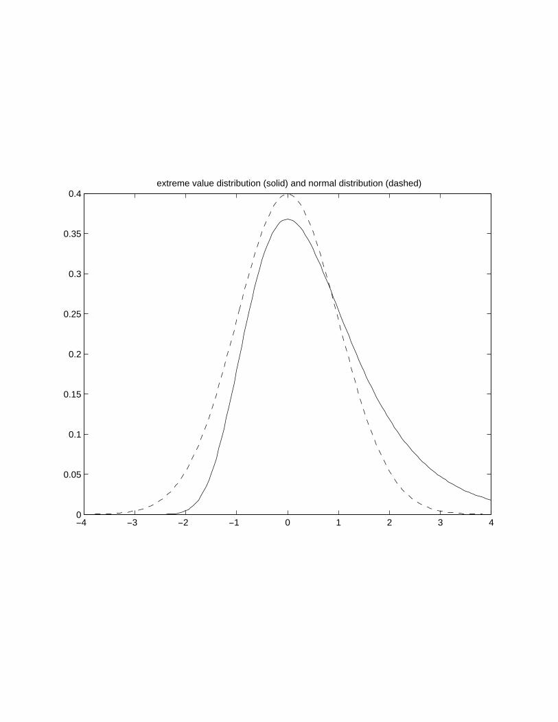
−4 −3 −2 −1 0 1 2 3 40
0.05
0.1
0.15
0.2
0.25
0.3
0.35
0.4extreme value distribution (solid) and normal distribution (dashed)
Imbens/Wooldridge, Lecture Notes 11, NBER, Summer ’07 6
=
∫ ∞
−∞
exp(−η + c) · exp(− exp(−η))dη
= exp(c) ·
∫ ∞
−∞
exp(−η) · exp(− exp(−η))dη = exp(c),
by change of variables, which we apply with
c = − ln (1 + exp(X ′i1β − X ′
i0β) + . . . + exp(X ′iJβ −X ′
i0β)) .
3. Independence of Irrelevant Alternatives
The main problem with the conditional logit is the property of Independence of Irrelevant
Alternative (IIA). Consider the conditional probability of choosing j given that you choose
either j or l:
Pr(Yi = j|Yi ∈ j, l) =Pr(Yi = j)
Pr(Yi = j) + Pr(Yi = l)=
exp(X ′ijβ)
exp(X ′ijβ) + exp(X ′
ilβ).
This probability does not depend on the characteristics Xim of alternatives m other than j
and l. This is sometimes unattractive. The traditional example is McFadden’s famous blue
bus/red bus example. Suppose there are initially three choices: commuting by car, by red
bus or by blue bus. It would seem reasonable be to assume that people have a preference
over cars versus buses, but are indifferent between red versus blue buses. One could capture
this by assuming that
Ui,redbus = Ui,bluebus,
with the choice between the blue and red bus being random. So, to be explicit, suppose that
Xi,bluebus = Xi,redbus = Xi,bus. Then suppose that the probability of commuting by bus is
Pr(Yi = bus) = Pr(Yi = redbus or bluebus) =exp(X ′
i,busβ)
exp(X ′i,bus
β) + exp(X ′i,carβ)
,
Imbens/Wooldridge, Lecture Notes 11, NBER, Summer ’07 7
and the probability of choosing a red bus or blue bus, conditional on choosing a bus, is
Pr(Yi = redbus|Yi = bus) =1
2.
That would imply that the conditional probability of commuting by car, given that one
commutes by car or red bus, would differ from the same conditional probability if there is
no blue bus. Presumably taking away the blue bus choice would lead all the current blue
bus users to shift to the red bus, and not to cars.
The conditional logit model does not allow for this type of substitution pattern. Another
way of stating the problems with the conditional logit model is to say that it generates
unrealistic substitution patterns. Let us make that argument more specific. Suppose that
individuals have the choice out of three Berkeley restaurants, Chez Panisse (C), Lalime’s (L),
and the Bongo Burger (B). Suppose the two characteristics of the restaurants are price with
PC = 95, PL = 80, and PB = 5, and quality, with QC = 10, QL = 9, and QB = 2. Suppose
that market shares for the three restaurants are SC = 0.10, SL = 0.25, and SB = 0.65. These
numbers are roughly consistent with a conditional logit model where the utility associated
with individual i and restaurant j is
Uij = −0.2 · Pj + 2 · Qj + εij,
with independent extreme value εij, and individuals go to the restaurant with the highest
utility. Now suppose that we raise the price at Lalime’s to 1000 (or raise it to infinity,
corresponding to taking it out of business). In that case the prediction of the conditional
logit model is that the market shares for Chez Panisse and the Bongo Burger go to SC = 0.13
and SB = 0.87. That seems implausible. The people who were planning to go to Lalime’s
would appear to be more likely to go to Chez Panisse if Lalime’s is closed than to go to the
Bongo Burger, and so one would expect SC ≈ 0.35 and SB ≈ 0.65. The model on the other
hand predicts that most of the individuals who would have gone to Lalime’s will now dine
(if that is the right term) at the Bongo Burger.
Imbens/Wooldridge, Lecture Notes 11, NBER, Summer ’07 8
Recall the latent utility set up with the utility for individual i and choice j equal to
Uij = X ′ijβ + εij. (2)
In the conditional logit model we assume independent εij with extreme value distributions.
This is essentially what creates the IIA property. (This is not completely correct, because
other distributions for the unobserved, say with normal errors, we would not get IIA exactly,
but something pretty close to it.) The solution is to allow in some fashion for correlation
between the unobserved components in the latent utility representation. In particular, with
a choice set that contains multiple versions of essentially the same choice (like the red bus
or the blue bus), we should allow the latent utilities for these choices to be identical, or at
least very close. In order to achieve this the unobserved components of the latent utilities
would have to be highly correlated for those choices. This can be done in a number of ways.
4. Models without Independence of Irrelevant Alternatives
Here we discuss three ways of avoiding the IIA property. All can be interpreted as relax-
ing the independence between the unobserved components of the latent utility. All of these
originate in some form or another in McFadden’s work (e.g., McFadden, 1981, 1982, 1984).
The first is the nested logit model where the researcher groups together sets of choices. In
the simple version with a single layer of nests this allows for non-zero correlation between
unobserved components of choices within a nest and maintains zero correlation between the
unobserved components of choices in different nests. Second, the unrestricted multinomial
probit model with no restrictions on the covariance between unobserved components, beyond
normalizations. Third, the mixed or random coefficients logit where the marginal utilities
associated with choice characteristics are allowed to vary between individuals. This gener-
ates positive correlation between the unobserved components of choices that are similar in
observed choice characteristics.
4.1 Nested Logit
One way to induce correlation between the choices is through nesting them. Suppose the
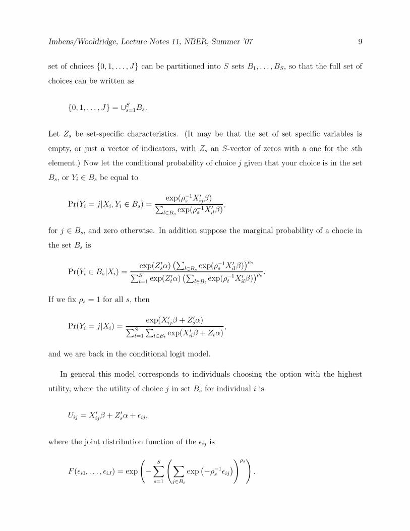
Imbens/Wooldridge, Lecture Notes 11, NBER, Summer ’07 9
set of choices 0, 1, . . . , J can be partitioned into S sets B1, . . . , BS, so that the full set of
choices can be written as
0, 1, . . . , J = ∪Ss=1Bs.
Let Zs be set-specific characteristics. (It may be that the set of set specific variables is
empty, or just a vector of indicators, with Zs an S-vector of zeros with a one for the sth
element.) Now let the conditional probability of choice j given that your choice is in the set
Bs, or Yi ∈ Bs be equal to
Pr(Yi = j|Xi, Yi ∈ Bs) =exp(ρ−1
s X ′ijβ)∑
l∈Bsexp(ρ−1
s X ′ilβ)
,
for j ∈ Bs, and zero otherwise. In addition suppose the marginal probability of a chocie in
the set Bs is
Pr(Yi ∈ Bs|Xi) =exp(Z ′
sα)(∑
l∈Bsexp(ρ−1
s X ′ilβ))ρs
∑S
t=1exp(Z ′
tα)(∑
l∈Btexp(ρ−1
t X ′ilβ))ρs
.
If we fix ρs = 1 for all s, then
Pr(Yi = j|Xi) =exp(X ′
ijβ + Z ′sα)
∑S
t=1
∑l∈Bt
exp(X ′ilβ + Ztα)
,
and we are back in the conditional logit model.
In general this model corresponds to individuals choosing the option with the highest
utility, where the utility of choice j in set Bs for individual i is
Uij = X ′ijβ + Z ′
sα + εij,
where the joint distribution function of the εij is
F (εi0, . . . , εiJ) = exp
(−
S∑
s=1
(∑
j∈Bs
exp(−ρ−1
s εij
))ρs)
.
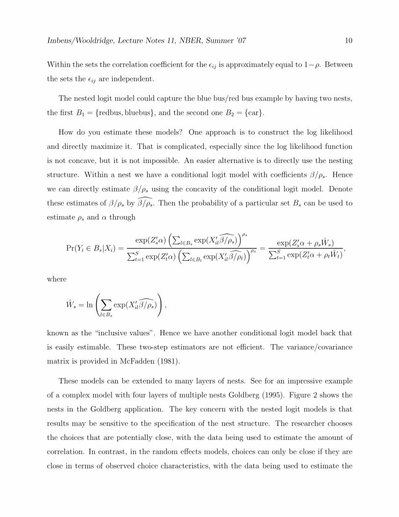
Imbens/Wooldridge, Lecture Notes 11, NBER, Summer ’07 10
Within the sets the correlation coefficient for the εij is approximately equal to 1−ρ. Between
the sets the εij are independent.
The nested logit model could capture the blue bus/red bus example by having two nests,
the first B1 = redbus, bluebus, and the second one B2 = car.
How do you estimate these models? One approach is to construct the log likelihood
and directly maximize it. That is complicated, especially since the log likelihood function
is not concave, but it is not impossible. An easier alternative is to directly use the nesting
structure. Within a nest we have a conditional logit model with coefficients β/ρs. Hence
we can directly estimate β/ρs using the concavity of the conditional logit model. Denote
these estimates of β/ρs by β/ρs. Then the probability of a particular set Bs can be used to
estimate ρs and α through
Pr(Yi ∈ Bs|Xi) =exp(Z ′
sα)(∑
l∈Bsexp(X ′
ilβ/ρs))ρs
∑S
t=1exp(Z ′
tα)(∑
l∈Btexp(X ′
ilβ/ρt))ρs
=exp(Z ′
sα + ρsWs)∑S
t=1exp(Z ′
tα + ρtWt),
where
Ws = ln
(∑
l∈Bs
exp(X ′ilβ/ρs)
),
known as the “inclusive values”. Hence we have another conditional logit model back that
is easily estimable. These two-step estimators are not efficient. The variance/covariance
matrix is provided in McFadden (1981).
These models can be extended to many layers of nests. See for an impressive example
of a complex model with four layers of multiple nests Goldberg (1995). Figure 2 shows the
nests in the Goldberg application. The key concern with the nested logit models is that
results may be sensitive to the specification of the nest structure. The researcher chooses
the choices that are potentially close, with the data being used to estimate the amount of
correlation. In contrast, in the random effects models, choices can only be close if they are
close in terms of observed choice characteristics, with the data being used to estimate the
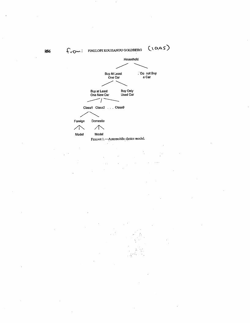
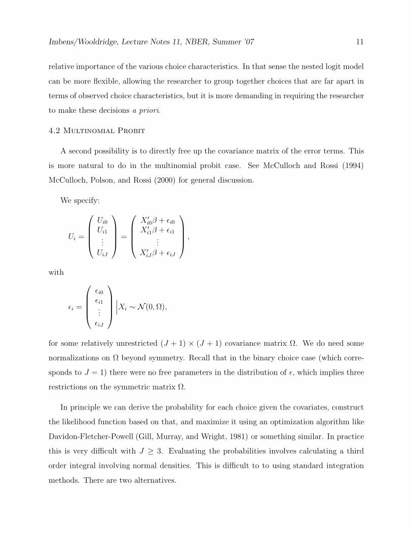
Imbens/Wooldridge, Lecture Notes 11, NBER, Summer ’07 11
relative importance of the various choice characteristics. In that sense the nested logit model
can be more flexible, allowing the researcher to group together choices that are far apart in
terms of observed choice characteristics, but it is more demanding in requiring the researcher
to make these decisions a priori.
4.2 Multinomial Probit
A second possibility is to directly free up the covariance matrix of the error terms. This
is more natural to do in the multinomial probit case. See McCulloch and Rossi (1994)
McCulloch, Polson, and Rossi (2000) for general discussion.
We specify:
Ui =
Ui0
Ui1
...UiJ
=
X ′i0β + εi0
X ′i1β + εi1
...X ′
iJβ + εiJ
,
with
εi =
εi0
εi1
...εiJ
∣∣∣Xi ∼ N (0, Ω),
for some relatively unrestricted (J + 1) × (J + 1) covariance matrix Ω. We do need some
normalizations on Ω beyond symmetry. Recall that in the binary choice case (which corre-
sponds to J = 1) there were no free parameters in the distribution of ε, which implies three
restrictions on the symmetric matrix Ω.
In principle we can derive the probability for each choice given the covariates, construct
the likelihood function based on that, and maximize it using an optimization algorithm like
Davidon-Fletcher-Powell (Gill, Murray, and Wright, 1981) or something similar. In practice
this is very difficult with J ≥ 3. Evaluating the probabilities involves calculating a third
order integral involving normal densities. This is difficult to to using standard integration
methods. There are two alternatives.
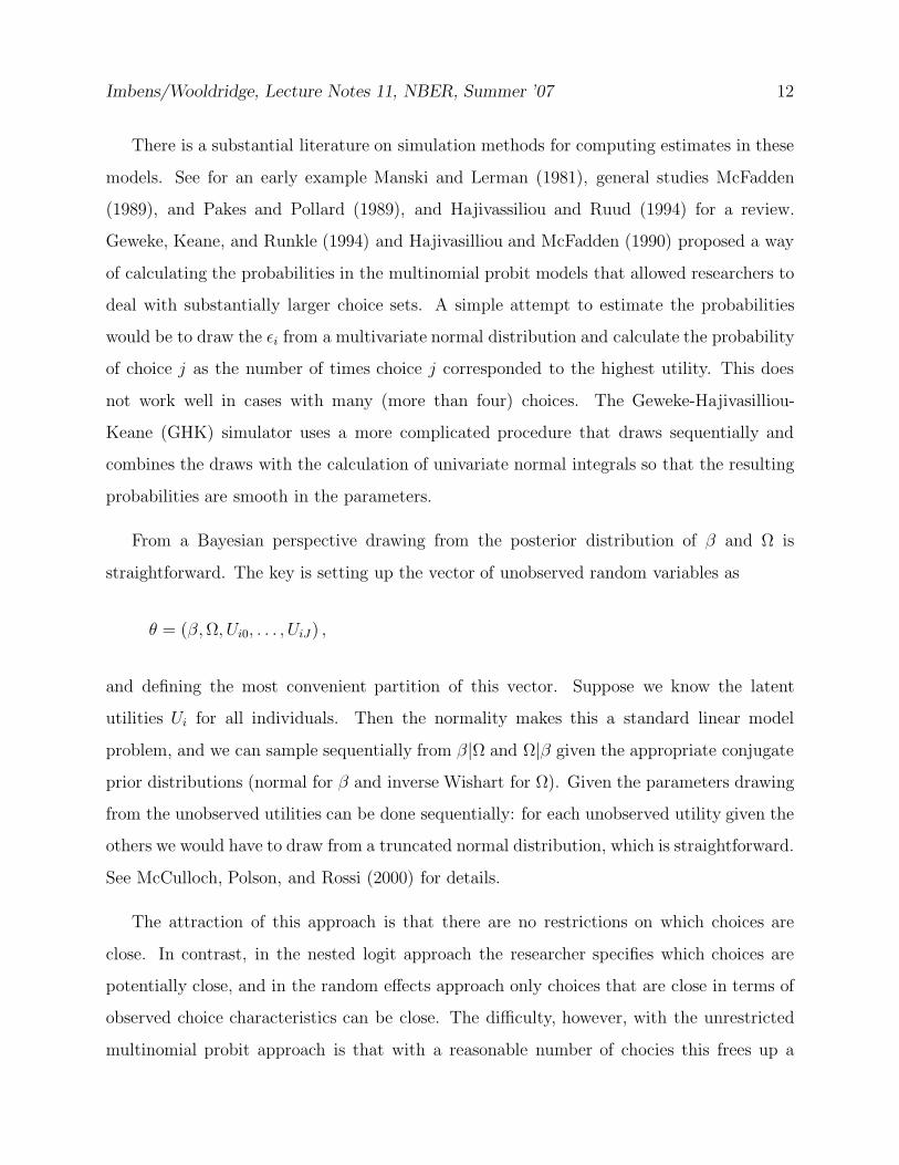
Imbens/Wooldridge, Lecture Notes 11, NBER, Summer ’07 12
There is a substantial literature on simulation methods for computing estimates in these
models. See for an early example Manski and Lerman (1981), general studies McFadden
(1989), and Pakes and Pollard (1989), and Hajivassiliou and Ruud (1994) for a review.
Geweke, Keane, and Runkle (1994) and Hajivasilliou and McFadden (1990) proposed a way
of calculating the probabilities in the multinomial probit models that allowed researchers to
deal with substantially larger choice sets. A simple attempt to estimate the probabilities
would be to draw the εi from a multivariate normal distribution and calculate the probability
of choice j as the number of times choice j corresponded to the highest utility. This does
not work well in cases with many (more than four) choices. The Geweke-Hajivasilliou-
Keane (GHK) simulator uses a more complicated procedure that draws sequentially and
combines the draws with the calculation of univariate normal integrals so that the resulting
probabilities are smooth in the parameters.
From a Bayesian perspective drawing from the posterior distribution of β and Ω is
straightforward. The key is setting up the vector of unobserved random variables as
θ = (β, Ω, Ui0, . . . , UiJ ) ,
and defining the most convenient partition of this vector. Suppose we know the latent
utilities Ui for all individuals. Then the normality makes this a standard linear model
problem, and we can sample sequentially from β|Ω and Ω|β given the appropriate conjugate
prior distributions (normal for β and inverse Wishart for Ω). Given the parameters drawing
from the unobserved utilities can be done sequentially: for each unobserved utility given the
others we would have to draw from a truncated normal distribution, which is straightforward.
See McCulloch, Polson, and Rossi (2000) for details.
The attraction of this approach is that there are no restrictions on which choices are
close. In contrast, in the nested logit approach the researcher specifies which choices are
potentially close, and in the random effects approach only choices that are close in terms of
observed choice characteristics can be close. The difficulty, however, with the unrestricted
multinomial probit approach is that with a reasonable number of chocies this frees up a
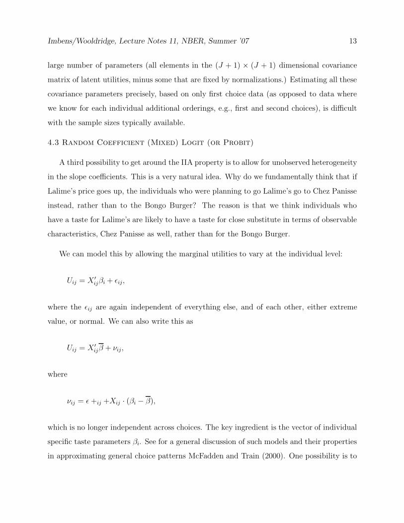
Imbens/Wooldridge, Lecture Notes 11, NBER, Summer ’07 13
large number of parameters (all elements in the (J + 1) × (J + 1) dimensional covariance
matrix of latent utilities, minus some that are fixed by normalizations.) Estimating all these
covariance parameters precisely, based on only first choice data (as opposed to data where
we know for each individual additional orderings, e.g., first and second choices), is difficult
with the sample sizes typically available.
4.3 Random Coefficient (Mixed) Logit (or Probit)
A third possibility to get around the IIA property is to allow for unobserved heterogeneity
in the slope coefficients. This is a very natural idea. Why do we fundamentally think that if
Lalime’s price goes up, the individuals who were planning to go Lalime’s go to Chez Panisse
instead, rather than to the Bongo Burger? The reason is that we think individuals who
have a taste for Lalime’s are likely to have a taste for close substitute in terms of observable
characteristics, Chez Panisse as well, rather than for the Bongo Burger.
We can model this by allowing the marginal utilities to vary at the individual level:
Uij = X ′ijβi + εij,
where the εij are again independent of everything else, and of each other, either extreme
value, or normal. We can also write this as
Uij = X ′ijβ + νij,
where
νij = ε +ij +Xij · (βi − β),
which is no longer independent across choices. The key ingredient is the vector of individual
specific taste parameters βi. See for a general discussion of such models and their properties
in approximating general choice patterns McFadden and Train (2000). One possibility is to
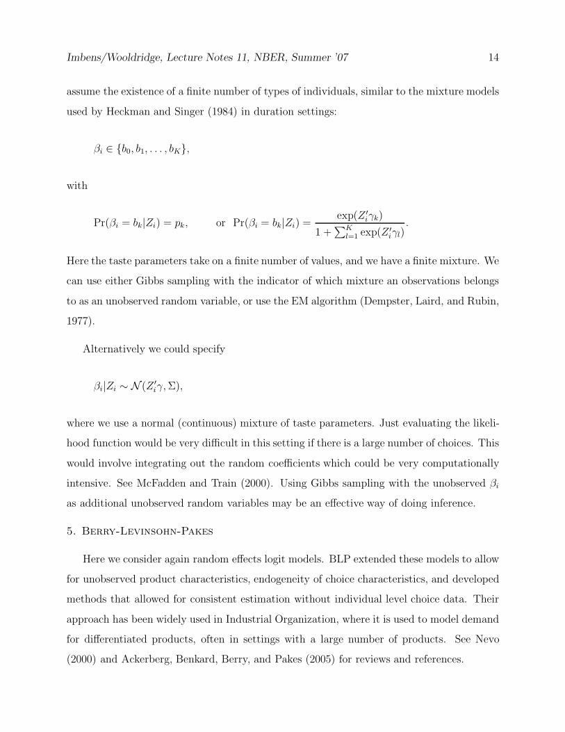
Imbens/Wooldridge, Lecture Notes 11, NBER, Summer ’07 14
assume the existence of a finite number of types of individuals, similar to the mixture models
used by Heckman and Singer (1984) in duration settings:
βi ∈ b0, b1, . . . , bK,
with
Pr(βi = bk|Zi) = pk, or Pr(βi = bk|Zi) =exp(Z ′
iγk)
1 +∑K
l=1exp(Z ′
iγl).
Here the taste parameters take on a finite number of values, and we have a finite mixture. We
can use either Gibbs sampling with the indicator of which mixture an observations belongs
to as an unobserved random variable, or use the EM algorithm (Dempster, Laird, and Rubin,
1977).
Alternatively we could specify
βi|Zi ∼ N (Z ′iγ, Σ),
where we use a normal (continuous) mixture of taste parameters. Just evaluating the likeli-
hood function would be very difficult in this setting if there is a large number of choices. This
would involve integrating out the random coefficients which could be very computationally
intensive. See McFadden and Train (2000). Using Gibbs sampling with the unobserved βi
as additional unobserved random variables may be an effective way of doing inference.
5. Berry-Levinsohn-Pakes
Here we consider again random effects logit models. BLP extended these models to allow
for unobserved product characteristics, endogeneity of choice characteristics, and developed
methods that allowed for consistent estimation without individual level choice data. Their
approach has been widely used in Industrial Organization, where it is used to model demand
for differentiated products, often in settings with a large number of products. See Nevo
(2000) and Ackerberg, Benkard, Berry, and Pakes (2005) for reviews and references.
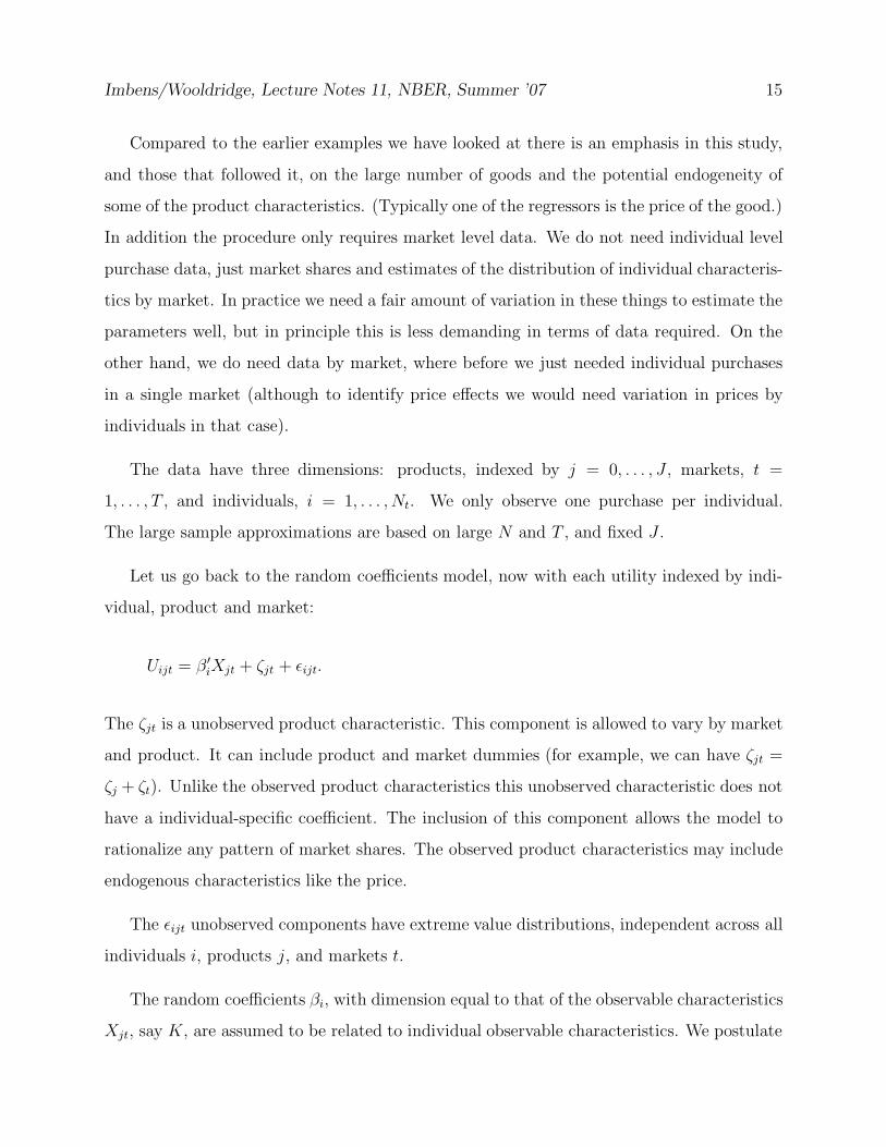
Imbens/Wooldridge, Lecture Notes 11, NBER, Summer ’07 15
Compared to the earlier examples we have looked at there is an emphasis in this study,
and those that followed it, on the large number of goods and the potential endogeneity of
some of the product characteristics. (Typically one of the regressors is the price of the good.)
In addition the procedure only requires market level data. We do not need individual level
purchase data, just market shares and estimates of the distribution of individual characteris-
tics by market. In practice we need a fair amount of variation in these things to estimate the
parameters well, but in principle this is less demanding in terms of data required. On the
other hand, we do need data by market, where before we just needed individual purchases
in a single market (although to identify price effects we would need variation in prices by
individuals in that case).
The data have three dimensions: products, indexed by j = 0, . . . , J , markets, t =
1, . . . , T , and individuals, i = 1, . . . , Nt. We only observe one purchase per individual.
The large sample approximations are based on large N and T , and fixed J .
Let us go back to the random coefficients model, now with each utility indexed by indi-
vidual, product and market:
Uijt = β ′iXjt + ζjt + εijt.
The ζjt is a unobserved product characteristic. This component is allowed to vary by market
and product. It can include product and market dummies (for example, we can have ζjt =
ζj + ζt). Unlike the observed product characteristics this unobserved characteristic does not
have a individual-specific coefficient. The inclusion of this component allows the model to
rationalize any pattern of market shares. The observed product characteristics may include
endogenous characteristics like the price.
The εijt unobserved components have extreme value distributions, independent across all
individuals i, products j, and markets t.
The random coefficients βi, with dimension equal to that of the observable characteristics
Xjt, say K, are assumed to be related to individual observable characteristics. We postulate
Imbens/Wooldridge, Lecture Notes 11, NBER, Summer ’07 16
the following linear form:
βi = β + Z ′iΓ + ηi,
with
ηi|Zi ∼ N (0, Σ).
So if the dimension of Zi is L× 1, then Γ is a L×K matrix. The Zi are normalized to have
mean zero, so that the β’s are the average marginal utilities. The normality assumption
is not necessary, and unlikely to be important. Other distributional assumptions can be
substituted.
BLP developed an approach to estimate models of this type that does not require in-
dividual level data. Instead it exploits aggregate (market level) data in combination with
estimates of the distribution of Zi. Specifically the data consist of estimated shares stj for
each choice j in each market t, combined with observations from the marginal distribution
of individual characteristics (the Zi’s) for each market, often from representative data sets
such as the CPS.
First write the latent utilities as
Uijt = δjt + νijt + εijt,
where
δjt = β ′Xjt + ζjt, and νijt = (Z ′iΓ + ηi)
′Xjt.
Now consider for fixed Γ and Σ and δjt the implied market share for product j in market
t, sjt. This can be calculated analytically in simple cases. For example with Γjt = 0 and
Σ = 0, the market share is a very simple function of the δjt:
sjt(δjt, Γ = 0, Σ = 0) =exp(δjt)∑Jl=0
exp(δlt).
Imbens/Wooldridge, Lecture Notes 11, NBER, Summer ’07 17
More generally, this is a more complex relationship. We can always calculate the implied
market share by simulation: draw from the distribution of Zi in market t, draw from the
distribution of ηi, and calculate the implied purchase probability (or even simulate the im-
plied purchase by also drawing from the distribution of εijt). Do that repeatedly and you
will be able to calculate the market share for this product/market. Call the vector function
obtained by stacking these functions for all products and markets s(δ, Γ, Σ).
Next, fix only Γ and Σ. For each value of δjt we can find the implied market share. Now
find the vector of δjt such that the implied market shares are equal to the observed market
shares sjt for all j, t. BLP suggest using the following algorithm. Given a starting value for
δ0jt, use the updating formula:
δk+1jt = δk
jt + ln sjt − ln sjt(δk, Γ, Σ).
BLP show this is a contraction mapping, and so it defines a function δ(s, Γ, Σ) expressing the
δ as a function of observed market shares, and parameters Γ and Σ. In order to implement
this, one needs to approximate the implied market shares accurately for each iteration in the
contraction mapping, and then you will need to do this repeatedly to get the contraction
mapping to converge.
Note that does require that each market share is accurately estimated. If all we have is
an estimated market share, then even if this is unbiased, the procedures will not necessarily
work. In that case the log of the estimated share is not unbiased for the log of the true share.
In practice the precision of the estimated market share is so much higher than that of the
other parameters that this is unlikely to matter.
Given this function δ(s, Γ, Σ) define the residuals
ωjt = δjt(s, Γ, Σ) − β ′Xjt.
At the true values of the parameters and the true market shares this is equal to the unob-
served product characteristic ζjt.
Imbens/Wooldridge, Lecture Notes 11, NBER, Summer ’07 18
Now we can use GMM or instrumental variable methods. We assume that the unobserved
product characteristics are uncorrelated with observed product characteristics (other than
typically price). This is not sufficient since the observed product characteristics enter directly
into the model. We need more instruments, and typically use things like characteristics of
other products by the same firm, or average characteristics by competing products. The
general GMM machinery will also give us the standard errors for this procedure. This is
where the method is most challenging. Finding values of the parameters that set the average
moments closest to zero can be difficult.
It is instructive to see what this approach does if we in fact have, and know we have, a
conditional logit model with fixed coefficients. In that case Γ = 0, and Σ = 0. Then we can
invert the market share equation to get the market specific unobserved choice-characteristics
δjt = ln sjt − ln s0t,
where we set δ0t = 0. (this is typically the outside good, whose average utility is normalized
to zero). The residual is
ζjt = δjt − β ′Xjt = ln sjt − ln s0t − β ′Xjt.
With a set of instruments Wjt, we run the regression
ln sjt − ln s0t = β ′Xjt + εjt,
using Wjt as instrument for Xjt, using as the observational unit the market share for product
j in market t.
So here the technique is very transparent. It amounts to transforming the market shares
to something linear in the coefficients so we can use two-stage-least-squares. More generally
the transformation is going to be much more difficult with the random coefficients implying
that there is no analytic solution. Computationally these things can get very complicated.
Note however that we can estimate these models now without having individual level data,
Imbens/Wooldridge, Lecture Notes 11, NBER, Summer ’07 19
and that at the same time we can get a fairly flexible model for the substitution patterns.
At the same time you would expect to need a lot of structure to get the parameters precisely
estimated just as in the other models. Of course if you compare the current model to the
nested logit model you can impose such structure by imposing restrictions on the covariance
matrix.
Comparisons of the models are difficult. Obviously if the structure imposed is correct it
helps, but we typically do not know what the truth is, so we cannot conclude which one is
better on the basis of the data typically available.
6. Models with Multiple Unobserved Choice Characteristics
The BLP approach allows for a single unobserved choice characteristic. This is essential
for their estimation strategy that requires only market share data, and exploits a one-to-one
relationship between market-specific unobserved product characteristics and market shares
given other parameters and covariates. With individual level data one may be able to, and
wish to allow for, multiple unobserved product characteristics. Elrod and Keane (1995),
Goettler and Shachar (2001), and Athey and Imbens (2007), among others, study such
models, in all cases with the unobserved choice characteristics constant across markets.
Athey and Imbens model the latent utility for individual i in market t for choice j as
Uijt = X ′itβi + ζ ′
jγi + εijt,
with the individual-specific taste parameters for both the observed and unobserved choice
characteristics normally distributed:
(βi
γi
)|Zi ∼ N (∆Zi, Ω).
Even in the case with all choice characteristics exogenous, maximum likelihood estimation
would be difficult. Athey and Imbens show that Bayesian methods, and in particular markov-
chain-monte-carlo methods are effective tools for conducting inference in these settings.
Imbens/Wooldridge, Lecture Notes 11, NBER, Summer ’07 20
7. Hedonic Models and the Motivation for a Choice and Individual Specific
Error Term
Recently researchers have reconsidered using pure characteristics models for discrete
choices, that is models with no idiosyncratic error εij, instead relying solely on the presence
of a few unobserved product characteristics and unobserved variation in taste parameters
to generate stochastic choices. Such an error term is the only source of stochastic variation
in the original multinomial choice models with only observed choice and individual charac-
teristics, but in models with unobserved choice and individual characteristics their presence
needs more motivation. Athey and Imbens (2007) discuss two arguments for including the
additive error term.
First, the pure characteristics model can be extremely sensitive to measurement error,
because it can predict zero market shares for some products. Consider a case where choices
are generated by a pure characteristics model that implies that a particular choice j has
zero market share. Now suppose that there is a single unit i for whom we observe, due to
measurement error, the choice Yi = j. Irrespective of the number of correctly measured ob-
servations available that were generated by the pure characteristics model, the estimates of
the latent utility function will not be close to the true values corresponding to the pure char-
acteristics model due to the single mismeasured observation. Such extreme sensitivity puts
a lot of emphasis on the correct specification of the model and the absence of measurement
error, and is undesirable in most settings.
Thus, one might wish to generalize the model to be robust against small amounts of
measurement error of this type. One possibility is to define the optimal choice Y ∗i as the
choice that maximizes the utility and assume that the observed choice Yi is equal to the
optimal choice Y ∗i with probability 1 − δ, and with probability δ/(J − 1) any of the other
choices is observed:
Pr(Yi = y|Y ∗i , Xi, νi, Z1, . . . , ZJ , ζ1, . . . , ζJ ) =
1 − δ if Y = Y ∗
i ,δ/(J − 1) if Y 6= Y ∗
i .
This nests the pure characteristics model (by setting δ = 0), without having the disad-
Imbens/Wooldridge, Lecture Notes 11, NBER, Summer ’07 21
vantages of extreme sensitivity to mismeasured choices that the pure characteristics model
has. If the true choices are generated by the pure characteristics model the presence of
a single mismeasured observation will not prevent the researcher from estimating the true
utility function. However, this specific generalization of the pure characteristics model has
an unattractive feature: if the optimal choice Y ∗i is not observed, all of the remaining choices
are equally likely. One might expect that choices with utilities closer to the optimal one are
more likely to be observed conditional on the optimal choice not being observed.
An alternative modification of the pure characteristics model is based on adding an
idiosyncratic error term to the utility function. This model will have the feature that,
conditional on the optimal choice not being observed, a close-to-optimal choice is more likely
than a far-from-optimal choice. Suppose the true utility is U∗ij but individuals base their
choice on the maximum of mismeasured version of this utility:
Uij = U∗ij + εij,
with an extreme value εij, independent across choices and individuals. The εij here can be
interpreted as an error in the calculation of the utility associated with a particular choice.
This model does not directly nest the pure characteristics model, since the idiosyncratic error
term has a fixed variance. However, it approximately nests it in the following sense. If the
data are generated by the pure characteristics model with the utility function g(x, ν, z, ζ),
then the model with the utility function λ · g(x, ν, z, ζ) + εij leads, for sufficiently large λ, to
choice probabilities that are arbitrarily close to the true choice probabilities (e.g., Berry and
Pakes, 2007).
Hence, even if the data were generated by a pure characteristics model, one does not lose
much by using a model with an additive idiosyncratic error term, and one gains a substantial
amount of robustness to measurement or optimization error.
Imbens/Wooldridge, Lecture Notes 11, NBER, Summer ’07 22
References
Ackerberg, D., L. Benkard, S. Berry, and A. Pakes, (2005), “Econometric Tools
for Analyzing Market Outcomes,” forthcoming, Handbook of Econometrics, Vol 5, Heckman
and Leamer (eds.)
Amemiya, T., and F. Nold, (19750, “A Modified Logit Model,” Review of Economics
and Statistics, Vol 57(2), 255-257.
Athey, S., and G. Imbens, (2007), “Discrete Choice Models with Multiple Unobserved
Product Characteristics,” International Economic Review, forthcoming.
Bajari, P., and L. Benkard, (2004), “Demand Estimation with Heterogenous Con-
sumers and Unobserved Product Characteristics: A Hedonic Approach,” Stanford Business
School.
Berry, S., (1994), “Estimating Discrete-Choice Models of Product Differentiation,”RAND
Journal of Economics, Vol. 25, 242-262.
Berry, S., J. Levinsohn, and A. Pakes, (1995), “Automobile Prices in Market
Equilibrium,” Econometrica, Vol. 63, 841-890.
Berry, S., J. Levinsohn, and A. Pakes (2004), “Differentiated Products Demand
Systems from a Combination of Micro and Macro Data: The New Car Market,” Journal of
Political Economy, Vol 112(1), 68-105.
Berry, S., O. Linton, and A. Pakes, (2004), “Limit Theorems for Estimating the
Parameters of Differentiated Product Demand Systems ”, Review of Economic Studies, Vol.
71, 613-654.
Berry, S., and A. Pakes, (2007), “The Pure Characteristics Discrete Choice Model
of Differentiated Products Demand,”International Economic Review, forthcoming.
Dempster, A., N. Laird, and D. Rubin, (1974), “Maximum Likelihood from In-
complete Data via the EM Algorithm”, (with discussion), Journal of the Royal Statistical

Imbens/Wooldridge, Lecture Notes 11, NBER, Summer ’07 23
Society, Series B, Vol. 39, 1-38.
Elrod, T., and M. Keane, (1995), “A Factor-Analytic Probit Model for Representing
the Market Structure in Panel Data, ”Journal of Marketing Research, Vol. XXXII, 1-16.
Geweke, J., M. Keane, and D. Runkle, (1994), “Alternative Computational Ap-
proaches to Inference in the Multinomial Probit Model,” Review of Economics and Statistics,
76, No 4, 609-632.
Gill, P., W. Murray, and M. Wright, (1981), Practical Optimization, Harcourt
Brace and Company, London
Goettler, J., and R. Shachar (2001), “Spatial Competition in the Network Televi-
sion Industry,” RAND Journal of Economics, Vol. 32(4), 624-656.
Goldberg, P., (1995), “Product Differentiation and Oligopoly in International Markets:
The Case of the Automobile Industry,” Econometrica, 63, 891-951.
Hajivassiliou, V., and P. Ruud, (1994), “Classical Estimation Methods for LDV
Models Using Simulation,” in Engle and McFadden 9eds.), Handbook of Econometrics, Vol
4, Chapter 40, Elseviers.
Hajivassiliou, V., and D. McFadden, (1990, “The method of simulated scores,”,
with application to models of external debt crises,” unpublished manuscript, Department of
Economics, Yale University.
Heckman, J., and B. Singer, (1984), “A Method for Minimizing the Impact of Dis-
tributional Assumptions in Econometric Models for Duration Data,” Econometrica, 52(2).
Manski, C., and S. Lerman,, (1981) “On the Use of Simulated Frequencies to Ap-
proximate Choice Probabilities,” in Structural Analysis of Discrete Data with Econometric
Applications, Manski and McFadden (eds.), 305-319, MIT Press, Cambridge, MA.
McCulloch, R., and P. Rossi, (1994) “An Exact Likelihood Analysis of the Multi-
nomial Probit Model, ”Journal of Econometrics 64 207-240.
Imbens/Wooldridge, Lecture Notes 11, NBER, Summer ’07 24
McCulloch, R., N. Polson, and P. Rossi, (2000) “A Bayesian Analysis of the
Multinomial Probit Model with Fully Identified Parameters, ”Journal of Econometrics 99,
173-193.
McFadden, D., (1973), “Conditional Logit Analysis of Qualitative Choice Behavior ”in
P. Zarembka (ed), Frontiers in Econometrics Academic Press, New York 105-142.
McFadden, D., (1981) “Econometrica Models of Probabilistic Choice,” in Structural
Analysis of Discrete Data with Econometric Applications, Manski and McFadden (eds.),
198-272, MIT Press, Cambridge, MA.
McFadden, D., (1982), “Qualitative Response Models,” in Hildenbrand (ed.), Advances
in Econometrics, Econometric Society Monographs, Cambridge University Press.
McFadden, D., (1984), “Econometric Analysis of Qualitative Response Models,”in
Griliches and Intriligator (eds), Handbook of Econometrics, Vol. 2, 1395- 1457, Amsterdam.
McFadden, D., (1989), “A Method of Simulated Moments for Estimation of Discrete
Response Models Without Numerical Integration,” Econometrica, 57(5), 995-1026.
McFadden, D., and K. Train, (2000), “Mxed MNL Models for Discrete Response,”
Journal of Applied Econometrics, 15(5), 447-470.
Nevo, A. (2000), “A Practioner’s Guide to Estimation of Random-Coefficient Logit
Models of Demand,” Journal of Economics & Management Science, Vol. 9, No. 4, 513-548.
Pakes, A., and D. Pollard, (1989), “Simulation and the Asymptotics of Optimization
Estimators,” Econometrica, 57(5), 1027-1057.
Imbens/Wooldridge, Lecture Notes 12, Summer ’07
What’s New in Econometrics? NBER, Summer 2007Lecture 12, Wednesday, August 1st, 11-12.30 pm
Missing DataThese notes discuss various aspects of missing data in both pure cross section and panel
data settings. We begin by reviewing assumptions under which missing data can be ignoredwithout biasing estimation or inference. Naturally, these assumptions are tied to “exogenous”sampling.
We then consider three popular solutions to missing data: inverse probability weighting,imputation, and Heckman-type selection corrections. The first to methods maintain “missing atrandom” or “ignorability” or “selection on observables” assumptions. Heckman corrections,whether applied to cross section data or panel data, linear models or (certain) nonlinearmodels, allow for “selection on unobservables.” Unfortunately, their scope of application islimited. An important finding is that all methods can cause more harm than good if selection ison conditioning variables that are unobserved along with response variables.1. When Can Missing Data be Ignored?
It is easy to obtain conditions under which we can ignore the fact that certain variables forsome observations, or all variables for some observations, have missing values. Start with alinear model with possibly endogenous explanatory variables:
yi xi ui, (1.1)
where xi is 1 K and the instruments zi are 1 L, L ≥ K. We model missing data with aselection indicator, drawn with each i. The binary variable si is defined as si 1 if we can useobservation i, si 0 if we cannot (or do not) use observation i. In the L K case we use IV onthe selected sample, which we can write as
IV N−1∑i1
N
sizi′xi
−1
N−1∑i1
N
sizi′yi
N−1∑i1
N
sizi′xi
−1
N−1∑i1
N
sizi′ui
(1.2)
(1.3)
For consistency, we essentially need
rank Esizi′xi K (1.4)
and
Esizi′ui 0, (1.5)
1
Imbens/Wooldridge, Lecture Notes 12, Summer ’07
which holds if Ezi′ui|si 0, which in turn is implied by
Eui|zi, si 0. (1.6)
Sufficient for (1.6) is
Eui|zi 0, si hzi (1.7)
for some function h. Note that the zero covariance assumption, Ezi′ui 0, is not sufficient
for consistency when si hzi. A special case is when Eyi|xi xi and selection si is afunction of xi. Provided the selected sample has sufficient variation in x, can consistentlyestimate by OLS on the selected sample.
We can use similar conditions for nonlinear models. What is sufficient for consistency onthe selected sample?
(Linear or Nonlinear) Least Squares: Ey|x, s Ey|x.Least Absolute Deviations: Medy|x, s Medy|xMaximum Likelihood: Dy|x, s Dy|x.
All of these allow selection on x but not generally on y (or unobservables that affect y).In the statistics literature, just using the data for which we observe all of yi,xi, zi (or just
yi,xi without instruments) is called the “complete case method.” In cases where we modelsome feature of Dy|x, it is clear that the richer is x, the more likely ignoring selection will notbias the results. In the case of estimating unconditional moments, say Eyi, unbiasednessand consistency of the sample on the selected sample requires Ey|s Ey.
Similar conditions can be obtained for panel data. For example, if we model Dyt|xt, andst is the indicator equal to one if xt,yt is observed, then the condition sufficient to ignoreselection is
Dst|xt,yt Dst|xt, t 1, . . . ,T. (1.8)
If, for example, xt contains yt−1, then selection is allowed to depend on the lagged responseunder (1.8). To see that (1.8) suffices, let the true conditional density be ftyit|xit,. Then thepartial log-likelihood function for a random draw i from the cross section can be written as
∑t1
T
sit log ftyit|xit,g ≡ ∑t1
T
sitlitg. (1.9)
Except for ensuring identifiability of , it suffices to show that Esitlit ≥ Esitlitg for allg ∈ Γ (the parameter space). But by a well-known result from MLE theory – theKulback-Leibler information inequality – maximizes Elitg|xit for all xit. But
2
Imbens/Wooldridge, Lecture Notes 12, Summer ’07
Esitlitg|xit EEsitlitg|yit,xit|xit EEsit|yit,xitlitg|xit
EEsit|xitlitg|xit Esit|xitElitg|xit,
where we used Esit|yit,xit Esit|xit from (1.8). Because Esit|xit Psit 1|xit ≥ 0, itfollows that Esitlit|xit ≥ Esitlitg|xit for all g ∈ Γ. Taking expectations of this inequalityand using iterated expectations gives the result. Thus, we have shown that maximizes theexpected value of each term in the summand in (1.9) – often not uniquely – and so it alsomaximizes the expected value of the sum. For identification, we have to assume it is the uniquemaximizer, as is usually the case of the model is identified in an unselected population and theselection scheme selects out “enough” of the population. One implication of this finding is thatselection is likely to be less of a problem in dynamic models where lags of y and lags of othercovariates appear, because then selection is allowed to be an arbitrary function of them. But,what is ruled out by (1.8) is selection that depends on idiosyncratic shocks to y between t − 1and t.
Methods to remove time-constant, unobserved heterogeneity deserve special attention.Suppose we have the linear model, written for a random draw i,
yit t xit ci uit. (1.10)
Suppose that we have instruments, say zit, for xit, including the possibility that zit xit. If weapply random effects IV methods on the unbalanced panel, sufficient for consistency (fixed T)are
Euit|zi1, . . . , ziT, si1, . . . , siT,ci 0, t 1, . . . ,T (1.11)
and
Eci|zi1, . . . , ziT, si1, . . . , siT Eci 0, (1.12)
along with a suitable rank condition. Somewhat weaker conditions suffice, but the generalpoint is that selection must be strictly exogenous with respect to the idiosyncratic errors as wellas the unobserved effect, ci. If we use the fixed effects estimator on the unbalanced panel, wecan get by with the first assumption, but, of course, all the instruments and selection to bearbitrarily correlated with ci. To see why, consider the just identified case and define, say,
ÿit yit − Ti−1∑r1
T siryir and similarly for and xit and zit, where Ti ∑r1T sir is the number of
time periods for observation i (properly viewed as random). The FEIV estimator is
3
Imbens/Wooldridge, Lecture Notes 12, Summer ’07
FEIV N−1∑i1
N
∑t1
T
sitzit′ xit
−1
N−1∑i1
N
∑t1
T
sitzit′ ÿit
N−1∑i1
N
∑t1
T
sitzit′ xit
−1
N−1∑i1
N
∑t1
T
sitzit′ uit .
Because zit is a function of zi1, . . . , ziT, si1, . . . , siT, (1.11) implies∑ t1T Esitzit
′ uit 0 (as do
weaker assumptions). There is a set of second moment assumptions that makes the usual,nonrobust inference procedures valid, but these impose homoskedasticity and serialindependence of the uit conditional on zi, si,ci.
There are some simple ways to test for selection bias in panel data applications. Oneimportant violation of (1.11) is when units drop out of the sample in period t 1 because ofshocks realized in time t. This generally induces correlation between si,t1 and uit. A simple testin the FE environment is to simply add si,t1 to the equation at time t, and estimate the resultingmodel by fixed effects (or FEIV). A simple t test can be used (probably fully robust). Of coursethe test entails dropping the last time period, and it need not have power for detectingcorrelation between sit and uit – that is, contemporaneous selection.
The consistency of FE (and FEIV) on the unbalanced panel under (1.11) breaks down if theslope coefficients are random but one ignores this in estimatin. That is, replace with bi butstill use the FE estimator. Then the error term contains the term xidi where di bi − . Ifselection is a function of di, then the usual FE estimator will be inconsistent. (Recall that theFE estimator, on balanced panels, has some robustness to random slopes.) A simple test is toallow di to be correlated with selection through the number of available time periods, Ti. Theidea is to consider alternatives with
Ebi|zi1, . . . , ziT, si1, . . . , siT Ebi|si1, . . . , siT Ebi|Ti. (1.13)
Then, add interaction terms of dummies for each possible sample size (with Ti T as the basegroup),
1Ti 2xit, 1Ti 3xit, ..., 1Ti T − 1xit (1.14)
to the equation and estimate it by FE. Significance of these interaction terms indicates thatrandom slopes are correlated with the available time periods, and suggests one might have toremove those random slopes (if possible).
If we first difference instead to remove ci – a method that has important advantages for
4
Imbens/Wooldridge, Lecture Notes 12, Summer ’07
attrition problems – we can apply the pooled IV results:
Δyit t Δxit Δuit, t 2, . . . ,T (1.15)
and, if zit is the set of IVs at time t, we can use
EΔuit|zit, sit 0 (1.16)
as being sufficient to ignore the missingess. Again, can add si,t1 to test for attrition.Not suprisingly, nonlinear models with unosberved effects are considerably more difficult
to handle, although certain conditional MLEs (logit, Poisson) can accomodate selection that isarbitrarily correlated with the unobserved effect.2. Inverse Probability Weighting2.1. Weighting with Cross-Sectional Data
A general solution to solving missing data problems when selection is not exogenous isbased on probability weights. To illustrate, for simplicity, suppose y is a random variablewhose population mean Ey we would like to estimate, but some observations aremissing on y. Let yi, si, zi : i 1, . . . ,N indicate independent, identically distributed drawsfrom the population, where zi is a vector that, for now, we assume is always observed. Supposewe assume the “selection on observables” assumption
Ps 1|y, z Ps 1|z ≡ pz (2.1)
where pz 0 for all possible values of z. Then we can solve the missing data problem byweighting the observed data points by 1/pzi:
IPW N−1∑i1
Nsi
pziyi, (2.2)
where note that si selects out the observed data points. It is easy to show, using iteratedexpectations, that IPW is not only consistent for yi, it is unbiased, too. (This same kind ofestimator arises in treatment effect estimation.) Of course, except in special cases, we mustestimate pzi; when zi is always observed along with si, flexible binary response models suchas logit or probit, or nonparametric methods, can be used. Let pzi denote the estimatedselection probability (also called the propensity score). Then an operational estimator is
IPW N−1∑i1
Nsi
pziyi. (2.3)
As written, this estimator assumes we know the size of the random sample, N, which is not
5
Imbens/Wooldridge, Lecture Notes 12, Summer ’07
necessarily the case for some sampling schemes, such as variable probability sampling. We canalso write IPW as
IPW N1−1N1/N∑
i1
Nsi
pziyi N1
−1∑i1
N
si
pziyi (2.4)
where N1 ∑ i1N si is the number of selected observations and N1/N is a consistent
estimate of Psi 1. The weights reported to account for missing data are often /pzi,which can be greater or less than unity. (By iterated expectatins, Epzi.) Equation (2.4)shows that IPW is a weighted average of the observed data points with weights /pzi. Yet adifferent estimator is obtained by solving the least squares problem
minm ∑i1
Nsi
pziyi − m2,
which results in
IPW ∑h1
Nsh
pzh
−1
∑i1
Nsi
pziyi , (2.5)
which is a different version a weighted.average.Horowitz and Manski (1998) have considered the problem of estimating population means
using IPW. Their main focus is on establishing bounds that do not rely on potentially strong,untestable assumptions such as the unconfoundedness assumption in (2.1). But they also note aparticular problem with certain IPW estimators even when the conditioning variable, x, isalways observed. They consider estimation of the mean Egy|x ∈ A for some set A. If wedefine di 1xi ∈ A then the problem is to estimate Egy|d 1. HM point out that, if oneuses the weights commonly reported with survey data – weights that do not condition on theevent d 1 – then the IPW estimate of the mean can lie outside the logically possible valuesof Egy|d 1. HM note that this problem can be fixed by using probability weightsPs 1|d 1/Ps 1|d 1, z unfortunately, this choice is not possible when data on x canalso be missing.
Failure to condition on d 1 when computing the probability weights when interest lies inEgy|d 1 is related to a general problem that arises in estimating models of conditionalmeans when data are missing on x. To see why, suppose the population regression function islinear:
6
Imbens/Wooldridge, Lecture Notes 12, Summer ’07
Ey|x x. (2.6)
Let z be a variables that are always observed and let pz be the selection probability, asbefore. Now, suppose that at least part of x is not always observed, so that x is not a subset of z.This means that some elements of x cannot appear in pz because pz normally has to beestimated using the data on si, zi for all i. The IPW estimator of solves
mina,b∑i1
Nsi
pziyi − a − xib2. (2.7)
Here is the problem: suppose that selection is exogenous in the sense that
Ps 1|x,y Ps 1|x. (2.8)
Then we saw in Section 1 that using least squares on the selected sample results in a consistentestimator of , ′ ′, which is also N -asymptotically normal. What about the weightedestimator? The problem is that if (2.8) holds, and z does not include x, then it is very unlikelythat
Ps 1|x,y, z Ps 1|z. (2.9)
In other words, the key unconfoundedness assumption fails, and the IPW estimator of isgenerally inconsistent. We actually introduce inconsistency by weighting when a standardunweighted regression on the complete cases would be consistent. In effect, the IPW estimatoruses weights that are functions of the wrong variables.
If x is always observed and can (and should) be included in z, then weighting is much moreattractive. Typically, z might contain lagged information, or interview information that wouldnot be included in x. If it turns out that selection is a function only of x, flexible estimation ofthe model Ps 1|z will pick that up in large sample sizes.
If x is always observed and we know that Ps 1|x,y Ps 1|x, is there any reason toweight by 1/px? If Ey|x x and Vary|x, weighting is asymptotically inefficient. IfEy|x x but Vary|x is heteroskedastic, then weighting may or may not be moreefficient than not. (The efficient estimator would be the WLS estimator that appropriatelyaccounts for Vary|x, different issue than probability weighting.) But both weighting and notweighting are consistent. The advantage of weighting is that, if the population “model” is infact just a linear projection, the IPW estimator consistently estimates that linear projectionwhile the unweighted estimator does not. In other words, if we write
7
Imbens/Wooldridge, Lecture Notes 12, Summer ’07
Ly|1,x ∗ x∗ (2.10)
where L| denotes the linear projection, then under Ps 1|x,y Ps 1|x, the IPWestimator is consistent for ∗. The unweighted estimator has a probabilty limit that depends onpx.
One reason to be interested in the LP is that the parameters of the LP show up in certaintreatment effect estimators. The notes on treatment effects contained a discussion of a “doublerobustness” result due to Robins and Ritov (1997); see also Wooldridge (2007). The idea isthis. In treatment effect applications, the ATE requires estimation of Eyg for the two
counterfactual outcomes, g 0,1). The LP has the property that Ey1 1∗ Ex1
∗, and so,if we consistently estimate 1
∗ and 1∗ then we can estimate Ey1 by averaging across x. A
similar statement holds for y0. Now, the IPW estimator identifies 1∗ and 1
∗ if the model forpx is correctly specified. But if Ey1|x 1 x1 then the IPW estimator is consistent for1 and 1 even if px is misspecified. And, of course, Ey1 1 Ex1. So, regardless ofwhether we are estimating the conditional mean parameters or the LP parameters, weconsistently estimate Ey1. The case where the IPW estimator does not consistently estimateEy1 is when Ey1|x is not linear and px is misspecified.
The double robustness result holds for certain nonlinear models, too, although one musttake care in combining the conditional mean function with the proper objective function –which, in this case, means quasi-log-likelihood function. The two cases of particular interestare the logistic response function for binary or fractional responses coupled with the BernoulliQLL, and the exponential response function coupled with the Poisson QLL.
Returning to the IPW regression estimator that solves (2.7), suppose we assume theignorability assumption (2.9),
Eu 0, Ex ′u 0,
pz Gz,
for a parametric function G (such as flexible logit), and is the binary response MLE. Then,as shown by Robins, Rotnitzky, and Zhou (1995) and Wooldridge (2007), the asymptoticvariance of IPW, using the estimated probability weights, is
Avar N IPW − Exi′xi−1Eriri
′Exi′xi−1, (2.11)
where ri is the P 1 vector of population residuals from the regression si/pzixi′ui on di
′,where di is the M 1 score for the MLE used to obtain . The asymptotic variance of IPW is
8
Imbens/Wooldridge, Lecture Notes 12, Summer ’07
easy to estimate:
∑i1
N
si/Gzi, xi′xi
−1
∑i1
N
riri′ ∑
i1
N
si/Gzi, xi′xi
−1
, (2.12)
or, if xi is always observed, the terms si/Gzi, can be dropped in the outer parts of the
sandwich. In the case that di is the score from a logit model of si on functions, say, hzi, di
has the simple form
di hi′si − hi, (2.13)
where a expa/1 expa and hi hzi. This illustrates a very interesting finding ofRobins, Rotnitzky, and Zhou (1995) and related to the Hirano, Imbens, and Ritter (2003)efficient estimator for means using IPW estimators. Suppose that, for a given set of functionshi1, the logit model is correctly specified in the sense that there is a 1 such thatPsi 1|zi hi11. Now suppose we take some additional functions of zi, sayhi2 h2zi, and add them to the logit. Then, asymptotically, the coefficients on hi2 are zero,and so the adjustment to the asumptotic variance comes from regressing si/hi11xi
′ui onhi1,hi2si − hi11. Now, notice that, even though the coefficients on hi2 are zero in thelogit model, the score vector depends on hi1,hi2. Therefore, the residual variance fromregressing si/hi11xi
′ui on hi1,hi2si − hi11 is generally smaller than that from usingthe correct logit model, which is obtained from regressing on hi1si − hi11. Byoverspecifying the logit model for si, we generally reduce the asymptotic variance of the IPWestimator. And the process does not stop there. We can keep adding functions of zi to the logitto reduce the asymptotic variance of the estimator of the IPW estimator. In the limit, if we havechosen the sequence of functions so that they approximate any well-behaved function, then weachieve asymptotic efficiency. This is precisly what the HIR estimator does by using a logitseries estimator for the propensity score.
Wooldridge (2007) shows that the adjustment to the asymptotic variance in (2.12) carriesover to general nonlinear models and estimation methods. One consequence is that ignoringthe estimation in pz – as commercial software typically does when specifying probabilityweights – results in conservative inference. But the adjustment to obtain the correct asymptoticvariance is fairly straightforward.
Nevo (2003) explicitly considers a generalized method of moments framework, and showshow to exploit known population moments to allow selection to depend on selected elements
9
Imbens/Wooldridge, Lecture Notes 12, Summer ’07
of the data vector w. (Hellerstein and Imbens (1998) use similar methods to improve estimationwhen population moments are known.) In particular, Nevo assumes that, along with themoment conditions Erw, 0, the population moments of the vector hw, say h, areknown. Under the assumption that selection depends on hw, that is,Ps 1|w Ps 1|hw, Nevo obtains an expanded set of moment conditions that can beused to estimate and the parameters in the selection equation. Suppose we use a logit modelfor Ps 1|hw. Then
E sihwi
rwi, 0 (2.14)
and
E sihwihwi
h. (2.15)
Equation (2.15) generally identifies , and then this can be used in a second step to choose to make the weighted sample moments
N−1∑i1
Nsi
hwirwi, (2.16)
as close to zero as possible. Because (2.15) adds as many moment restrictions as parameters,the GMM estimator using both sets of moment conditions is equivalent to the two-stepestimator just described.
Another situation where the missing data problem can be solved via weighting is when datahave been censored due to a censored duration. The response variable of interest may be theduration, or it may be a variable observed only if a duration or survival time is observed. Let ybe a univariate response and x a vector of conditioning variables, and suppose we are interestedin estimating Ey|x. A random draw i from the population is denoted xi, yi. Let ti 0 be aduration and let ci 0 denote a censoring time (where ti yi is allowed). Assume that xi, yi
is observed whenever ti ≤ ci, so that si 1ti ≤ ci. Under the assumption that ci isindependent of xi, yi, ti,
Psi 1|xi,yi, ti Gti, (2.17)
where Gt ≡ Pci ≥ t. In order to use inverse probability weighting, we need to observe ti
whenever si 1, which simply means that ti is uncensored. Plus, we need only observe ci
when si 0. of ci. As shown in Wooldridge (2007), it is more efficient to estimate G using
10
Imbens/Wooldridge, Lecture Notes 12, Summer ’07
the density of minci, ti given ti. Generally, let hc, denote a parametric model for thedensity of the censoring times, ci, and let Gt, be the implied model for Pci ≥ t. The loglikelihood is
∑i1
N
1 − si loghci, si logGti,, (2.18)
which is just the log-likelihood for a standard censored estimation problem but where ti (theunderlying duration) plays the role of the censoring variable. As shown by Lancaster (1990 forgrouped duration data, where hc, is piecewise constant, the solution to (2.18) gives asurvivor function identical to the Kaplan-Meier estimator but where the roles of ci and ti arereversed; that is, we treat ti as censoring ci. The linear regression model has a long history, andhas been studied recently by Honoré, Khan, and Powell (2002). See also Rotnitzky and Robins(2005) for a survey of how to obtain semiparametrically efficient estimators. TheKoul-Susarla-van Ryzin (1981) estimator is an IPW least squares estimator, but their proposalsfor inference are very difficult to implement. As shown by Wooldridge (2007), this is anotherinstance where estimating the selection probability by MLE is more efficient than using theknown probability (if you could). Plus, obtaining the smaller variance matrix involves only amultivariate regression of the weighted score for the second stage problem – OLS, NLS, MLE,or IV – on the score for the first-stage Kaplan-Meier estimation. This simple procedure is validwhen the distribution of ci is taken to be discrete. Other authors undertake the asymptoticsallowing for an underlying continuous censoring time, which makes estimating asymptoticvariances considerably more difficult.
2.2 Attrition in Panel Data
Inverse probability weighting can be applied to solve, in some cases, the attrition problemin panel data. For concreteness, consider maximum pooled maximum likelihood, where wemodel a density ftyt|xt for any conditioning variables xt. These need not be strictlyexogenous or always observed. Let ftyt|xt, be the parametric model, and let sit be theselection indicator. We assume that attrition is absorbing, so sit 1 sir 1 for r t. Theestimator that ignores attrition solves
max∈Θ∑i1
N
∑t1
T
sit log ftyit|xit,, (2.19)
which is consistent if Psit 1|yit,xit Psit 1|xit. This follows by showing
11
Imbens/Wooldridge, Lecture Notes 12, Summer ’07
EPsit 1|xitElog ftyit|xit,|xit, and using the fact that the true value of maximizesElog ftyit|xit,|xit for all t, and Psit 1|xit ≥ 0. But, if selection depends on yit even afterconditioning on xit, the unweighted estimator is generally inconsistent. If wit xit,yit, thenperhaps we can find variables r it, such that
Psit 1|wit,r it Psit 1|r it ≡ pit 0, t 1, . . . ,T. (2.20)
(The “obvious” set of variables rit wit is not usually available since we will have estimatethe probabilities.) If we could observe the pit, we could use the weighted MLE,
max∈Θ∑i1
N
∑t1
T
sit/pit log ftyit|xit,, (2.21)
which we call w. The estimator w is generally consistent because
Esit/pitqtwit, Eqtwit,, t 1, . . . ,T, . (2.22)
where qtwit, log ftyit|xit, is the objective function.How do we choose r it to make (2.20) hold (if possible)? A useful strategy, considered by
RRZ, is to build the pit up in a sequential fashion. At time t, zit is a set of variables observedfor the subpopulation with si,t−1 1. (si0 ≡ 1 by convention). Let
it Psit 1|zit, si,t−1 1, t 1, . . . ,T. (2.23)
Typically, zit contains elements from wi,t−1, . . . ,wi1, and perhaps variables dated at t − 1 orearlier that do not appear in the population model. Unfortunately, zit rarely can depend ontime-varying variables that are observed in period t (since we have to apply a binary responsemodel for the sample with si,t−1 1, and this includes units that have left the sample at time t!)Given the monotone nature of selection, we can estimate models for it sequential when the zit
are observed for every unit in the sample at time t − 1.How do we obtain pit from the it? Not without some assumptions. Let
vit wit,zit, t 1, . . . ,T. An ignorability assumption that works is
Psit 1|vi1, . . . ,viT, si,t−1 1 Psit 1|zit, si,t−1 1, t ≥ 1. (2.24)
That is, given the entire history vi vi1, . . . ,viT, selection at time t (given being still in the
sample at t − 1) depends only on zit; in practice, this means only on variables observed at t − 1.This is a strong assumption; RRZ (1995) show how to relax it somewhat in a regressionframework with time-constant covariates. Using this assumption, we can show that
pit ≡ Psit 1|vi iti,t−1 i1. (2.25)
12
Imbens/Wooldridge, Lecture Notes 12, Summer ’07
In the general framework, we have r it zit, . . . ,zi1 but, because of the ignorability
assumption, it is as if we can take r it wi1,zi1, . . . , wiT,zit.
So, a consistent two-step method is:(1) In each time period, estimate a binary response model for Psit 1|zit, si,t−1 1,
which means on the group still in the sample at t − 1. The fitted probabilities are the it. Formpit iti,t−1 i1. Note that we are able to compute pit only for units in the sample at timet − 1.
(2) Replace pit with pit in (2.21), and obtain the weighted M-estimator.Consistency is straightforward – standard two-step estimation problem – if we have the
correct functional form and the ignorability of selection assumption holds. As shown by RRZ(1995) in the regression case, it is more efficient to estimate the pit than to use know weights,if we could. See RRZ (1995) and Wooldridge (2002) for a simple regression method foradjusting the score; it is similar to that used for the cross section case, but just pooled across t.
IPW for attrition suffers from a similar drawback as in the cross section case. Namely, ifPsit 1|wit Psit 1|xit then the unweighted estimator is consistent. If we use weightsthat are not a function of xit in this case, the IPW estimator is generally inconsistent: weightinguncessesarily causes inconsistency.
Related to the previous point is that it would be rare to apply IPW in the case of a modelwith completely specified dynamics. Why? Suppose, for example, we have a model ofEyit|xit,yi,t−1, . . . ,xi1,yi0. If our variables affecting attrition, zit, are functions ofyi,t−1, . . . ,xi1,yi0 – as they often must be – then selection is on the basis of conditioningvariables, and so the unweighted estimator is also consistent. RRZ (1995) explicitly coverregressions that do not have correct dynamics.3. Imputation
Section 1 discussed conditions under which dropping observations with any missing dataresults in consistent estimators. Section 2 showed that, under an unconfoundednessassumption, inverse probability weighting can be applied to the complete cases to recoverpopulation parameters. One problem with using IPW for models that contain covariates is thatthe weighting may actually hurt more than it helps if the covariates are sometimes missing andselection is largely a function of those covariates.
A different approach to missing data is to try to fill in the missing values, and then analyzethe resulting data set as a complete data set. Imputation methods, and multiple imputation use
13
Imbens/Wooldridge, Lecture Notes 12, Summer ’07
either means, fitted values, values or averages from “similar” observations, or draws fromposterior distributions to fill in the missing values. Little and Rubin (2002) provides anaccessible treatment with lots of references to work by Rubin and coauthors.
Naturally, such procedures cannot always be valid. Most methods depend on a missing atrandom (MAR) assumption. When data are missing on only one variable – say, the responsevariable, y – MAR is essentially the same as the unconfoundedness assumptionPs 1|y,x Ps 1|x. (The assumption missing completely at random (MCAR) is when sis independent of w x,y.) MAR can be defined for general missing data patterns. Forexample, in a bivariate case, let wi wi1,wi2 be a random draw from the population, wheredata can be missing on either variable. Let ri ri1, ri2 be the “retention” indicators for wi1
and wi2, so rig 1 implies wig is observed. The MCAR assumption is that ri is independent of
wi, so Dri|wi Dri. The MAR assumption is that impliesPri1 0, ri2 0|wi Pri1 0, ri2 0 ≡ 00, Pri1 1, ri2 0|wi1,Pri1 0, ri2 1|wi2, and thenPri1 1, ri2 1|wi 1 − 00 − Pri1 1, ri2 0|wi1 − Pri1 0, ri2 1|wi2. Even withjust two variables, the restrictions imposed by MAR are not especially appealing, unless, ofcourse, we have good reason to just assume MCAR.
MAR is more natural with monotone missing data problems, which sometime apply inpanel data situations with attrition. Order the wig so that if wih is observed the so is wig, g h.
Then the retention indicators satisfy rig 1 ri,g−1 1. Under MAR, the joint density
fw1, . . . ,wG is easy to estimate. Writefw1, . . . ,wG fwG|wG−1, . . . ,w1 fwG−1|wG−1, . . . ,w1fw2|w1fw1. Given parametricmodels, we can write partial log likelihood as
∑g1
G
rig log fwig|wi,g−1, . . . ,wi1,, (3.1)
where fw1|w0, ≡ fw1|w0,, and it suffices to multiply only by rig because
rig rigri,g−1ri2. Under MAR,
Erig|wig, . . . ,wi1 Erig|wi,g−1, . . . ,wi1, (3.2)
and so by (3.2),
Erig log fwig|wig−1|wi
g−1 Erig|wig−1Elog fwig|wi
g−1|wig−1. (3.3)
The first term on the RHS of (3.3) is Erig|wig−1 Prig 1|wi
g−1 ≥ 0 and the true value of
14
Imbens/Wooldridge, Lecture Notes 12, Summer ’07
maximizes the second part by the conditional Kullback-Leibler information inequality (forexample, Wooldridge (2002, Chapter 13)). Therefore, the parameters of the conditionaldensities are generally identified, provided the missing data problem is not too severe.
Before briefly describing how multiple imputation works, a simple example helps illustratethe general idea behind imputation. Suppose y is a random variable in a population with meany, but data are missing on some yi random drawn from the population. Let si be the binary
selection indicator, and let xi be a set of observed covariates. So, a random draw consists ofxi,yi, si but where yi is missing if si 0. As we discussed earlier, unless s is independent ofy – that is, the data are MCAR – the complete-case sample average,
y ∑i1
N
si
−1
∑i1
N
siyi, (3.4)
is not unbiased or consistent for y; its probability limit is, of course, Ey|s 1.
Suppose, however, that the selection is ignorable conditional on x:
Ey|x, s Ey|x mx,, (3.5)
where mx, is, for simplicity, a parametric function. As we discussed in Section 1, nonlinearleast squares, and a variety of quasi-MLEs, are consistent for using the selected sample.
Now, because we observe xi for all i, we can obtained fitted values, mxi, , for any unit it the
sample. Let ŷ i siyi 1 − simxi, be the imputed data. Then an imputation estimator ofy is
y N−1∑i1
N
siyi 1 − simxi, . (3.6)
The plim of y is easy to find by replacing with and sample average with the population
average:
Esiyi 1 − simxi, EEsiyi|xi, si E1 − simxi, EsiEyi|xi, si E1 − simxi, Esimxi, E1 − simxi, Emxi, y. (3.7)
(Of course, we could average the mxi, across all i, but that would throw away someinformation on the yi that we observe.)
If Dy|x, s Dy|x then we can use MLE on the complete cases, obtain estimates of the
15
Imbens/Wooldridge, Lecture Notes 12, Summer ’07
parameters, say , and then use mxi, as above, where mx, is the mean function impliedby the model for Dy|x. For example, y could be a corner solution response and then we use aTobit or some flexible extension for Dy|x.
One danger in using even simple imputation methods like the one just covered is that wewill ignore the errors in the imputed values. ŷ i differs from yi for two reasons. First, if we write
yi mxi, ui, (3.8)
then, even if we knew , the error would be ui. (In effect, we are replace yi with its conditionalexpectation.) Having to estimate further introduces estimation error. Analytical formulas canbe worked out, but bootstrapping a standard error or confidence interval for y is also
straightforward: we would draw observation indices at random, without replacement, andperform the imputation steps on each new bootstrap sample.
As an example of how just using the imputed values as if they were real data, suppose we
run a linear regression using the complete data and obtain xi. Again defining
ŷ i siyi 1 − sixi, suppose we use the imputed data set to reestimate . It is well known
that we just get back again. However, our estimated error variance will be too small becauseevery residual for an imputed data point is identically zero. It follows that, while SSR/N1 − Kis generally unbiased for u
2 (under the Gauss-Markov assumptions), where N1 is the numberof complete cases, SSR/N − K has a downward bias.
The previous method ignores the random error in (3.4); Little and Rubin (2002) call it themethod of “conditional means.” Generally, as they show in Table 4.1, the method ofconditional means results in downward bias in estimating variances. Instead, LR propose
adding a random draw to mxi, to impute a value. Of course, this entails have a distribution
from which to draw the ui. If we assume that ui is independent of xi and normally distributed,then we can draw, say, u i from a Normal0, u
2, distribution, where u2 is estimated using the
complete case nonlinear regression residuals. This procedure works well for estimating y2 in
the case where linear regression is used and xi,yi is jointly normal. LR refer to this as the“conditional draw” method of imputation, which is a special case of stochastic imputation.
Little and Rubin argue that the conditional draw approach, at least in the jointly normalcase, works well when a covariate is missing. Suppose that x x1,x2 and data are missingon x2 but not x1,y. One possibility for imputing xi2 when it is missing is to regress xi2 on xi1
using the complete cases, and then use fitted values, or conditional draws, to impute xi2. LRshow that the method of conditional draws (not conditional means) works well when y is
16
Imbens/Wooldridge, Lecture Notes 12, Summer ’07
included along with x1 in obtained the estimated conditional means from the complete-caseregression.
Unfortunately, except in simple cases, it is difficult to quantity the uncertainty fromsingle-imputation methods, where one imputed values is obtained for each missing variable.One possibility, which has been studied in the statistics literature, is to bootstrap the entireestimation method – assuming, of course, that the imputations eliminates the nonresponse bias(so that missing at random holds). In the example of conditional draws above, the imputationprocedure is simply included in any subsequent estimation, and bootstrap samples are obtainedover and over again. On each bootstrap replication, say b, an estimate of the parameters using
the complete cases, completeb is obtained (which would be the beta hats and error variance
estimate in the regression case), missing data values are imputed using conditional draws, and
then an estimate of using the imputed data, imputedb , can be obtained. Of course, this can be
computationally intensive for nonlinear estimation problems.An alternative is the method of multiple imputation. Its justification is Bayesian, and based
on obtaining the posterior distribution – in particular, mean and variance – of the parametersconditional on the observed data. For general missing data patterns, the computation requiredto impute missing values is quite complicated, and involves simulation methods of estimation.LR and Cameron and Trivedi (2005) provide discussion. But the idea is easily illustrated usingthe above example. Rather than just impute one set of missing values to create one “complete”data set, created several imputed data sets. (Often the number is fairly small, such as five orso.) Then, estimate the parameters of interest using each imputed data set, and then use anaveraging to obtain a final parameter estimate and sampling error.
Briefly, let Wmis denote the matrix of missing data and Wobs the matrix of observations.Assume that MAR holds. Then multiple imputation is justified as a way to estimate E|Wobs,the posterier mean of given Wobs. But by iterated expectations,
E|Wobs EE|Wobs,Wmis|Wobs. (3.9)
Now, if we can obtain estimates d E|Wobs,Wmisd for imputed data set d, then we can
approximate E|Wobs as
D−1∑d1
D
d, (3.10)
which is just the average of the parameter estimates across the imputed samples.
17
Imbens/Wooldridge, Lecture Notes 12, Summer ’07
Further, we can obtain a “sampling” variance by estimating Var|Wobs using
Var|Wobs EVar|Wobs,Wmis|Wobs VarE|Wobs,Wmis|Wobs, (3.11)
which suggests
Var|Wobs D−1∑d1
D
Vd D − 1−1∑d1
D
d − d − ′
≡ V B,
(3.12)
where V is the average of the variance estimates across imputed samples and B is thebetween-imputation variance. For small a small number of imputations, a correction is usuallymade, namely, V 1 D−1B. Therefore, assume that one trusts the MAR assumption, andthe underlying distributions used to draw the imputed values, inference with multipleimputations is fairly straightforward. Because D need not be very large, estimation ofnonlinear models using multiple imputations is not computationally prohibitive (once one hasthe imputed data, of course).
Like weighting methods, imputation methods have an important shortcoming when appliedto estimation of models with missing conditioning variables. Suppose again that x x1,x2,
we are interested in some feature of the conditional distribution Dy|x, data are missing on yand x2 – say, for the same units – and selection is a function of x2. Then, as we discussed inSection 1, MLE using the complete cases is consistent, asymptotically normal, and inference isstandard. What about imputation methods? Because they generally rely on MAR, they wouldrequire that Ds|y,x1,x2 Ds|x1. Because this is false in this example, MI cannot beexpected to produce convincing imputations.
Imputation for the monotone case discussed above is relatively straightforward underMAR, and MAR is at least plausible. Because the conditional densities are identified,imputation can proceed sequentially: given wi1 and , missing values on wi2 can be imputed bydrawing from f2|wi1, . Then, wi3 can be imputed by drawing from f|ŵi2,wi1, , where ŵi2
may or may not be imputed. And so on.4. Heckman-Type Selection Corrections4.1. Corrections with Instrumental Variables
Here we briefly cover the well-known Heckman selection correction with endogenousexplanatory variables in a linear model. The model is
18

Imbens/Wooldridge, Lecture Notes 12, Summer ’07
y1 z11 1y2 u1
y2 z2 v2
y3 1z3 v3 0.
(4.1) (4.2) (4.3)
where z is 1 L with first element unity (and also in z1). As usually, L1 L for identification.The key point to be made here is, depending on how the Heckman correction is carried out inthis case, (4.2) can just be a linear projection – in which case the nature of y2 is unrestricted –or, effectively, v2 must be normal and independent of z. Intuitively, we need two elements in znot also in z1: loosely, one to induce exogenous variation in y2 and the other to induceexogenous variation in selection. If we assume (a) z,y3 is always observed, y1,y2 observedwhen y3 1; (b) Eu1|z,v3 1v3; (c) v3|z ~Normal0,1; (d) Ez′v2 0 and 22 ≠ 0, thenwe can write
y1 z11 1y2 gz,y3 e1 (4.4)
where e1 u1 − gz,y3 u1 − Eu1|z,y3. So, selection is exogenous in (4.4) becauseEe1|z,y3 0. Because y2 is not exogenous, we estimate (4.4) by IV, using the selectedsample, where the instruments are z,z3 because gz, 1 z3. So, the two-stepestimator is
(i) Probit of y3 on z to (using all observations) to get i3 ≡ zi3
(ii) IV (2SLS if overidentifying restrictions) of yi1 on zi1,yi2, i3 using the selectedsample and instruments zi, i3.
If y2 is always observed, it is tempting to obtain the fitted values ŷ i2 from the reduced formyi2 on zi, and then use OLS of yi1 on zi1,ŷ i2, i3 in the second stage. But this effectively puts1v2 in the error term, so we would need u1 2v2 to be normal (or something similar); itwould not be consistent for discrete y2, for example. Implicitly, the reduced form estimated bythe proper two-step procedure is, on the selected sample, y2 z2 2z3 r3. But this isjust a linear projection; generally, the rank condition on the selected sample should hold if zcauses sufficient variation in y2 and y3 in the population.
This example raises another point: even if y2 is exogenous in the full population, oneshould generally treat it as endogenous in the selected subsample. Why? Because y2 cannot beincluded in the first-stage probit if it is not always observed, so consistency of the Heckmanprocedure would require Py3 1|z1,y2 Py3 1|z1, a tenuous assumption. Unless wehave an instrument for y2, simply treating it as exogenous in the second stage after omitting it
19
Imbens/Wooldridge, Lecture Notes 12, Summer ’07
from the first is tantamount to imposing an exclusion restriction on a reduced form.In addition to the linear model, with or without endogenous variables, Heckman-type
corrections are available for a limited set of nonlinear models. Terza (1998) contains theapproach for exponential functions with exogenous explanatory variables, where the selectionequation follows a probit; see also Wooldridge (2002, Chapter 19). A selection correction isalso fairly easy to implement in probit models, too; see Wooldridge (2002, Chapter 17). As intrying to account for endogenous explanatory variables in such models, merely inserting anestimated inverse Mills ratio inside, say, an exponential model, or probit model, or Tobitmodel. One can always base a test on a variable-addition approaches, but they cannot be shownto solve the selection problem.
A very similar issue arises when using Heckman’s method to correct for attrition in paneldata (when selection on observables does not hold). With attrition as an absorbing state, it iscommon to estimate models in first differences to remove additive heterogeneity, say
Δyit Δxit Δuit, t 2, . . . ,T. (4.5)
We assume sit 1 sir 1, r t. Let wit be a set of variables that we always observe whensi,t−1 1 such that wit is a good predictor of selection – in a sense soon to be made precise.We model the selection in time period t conditional on si,t1 1 as
sit 1wit t vit 0vit|wit, si,t−1 1~Normal0,1, t 2,3, . . . ,T.
(4.6) (4.7)
Since attrition is an absorbing state, sit−1 0 implies sit 0. This leads to a probit model forsit conditional on si,t−1 1 :
Psit 1|wit, si,t−1 1 wit t, t 2, . . . ,T. (4.8)
Naturally, we need to estimate t, which we do as a sequence of probits. For t 2, we use theentire sample to estimate a probit for still being in the sample in the second period. For t 3,we estimate a probit for those units still in the sample as of t 2. And so on. When we reacht T, we have the smallest group of observations because we only use units still in the sampleas of T − 1. Where might the wit come from? Since they have to be observed at time t for theentire subgroup with si,t−1 1, wit generally cannot contain variables dated at time t (unlesssome information is known at time t on people who attrit at time t). When the xit are strictlyexogenous, we can always include in wit elements of xi,t−1,xi,t−2, . . . ,xi1. Note that thepotential dimension of wit grows as we move ahead through time. Unfortunately, yi,t−1 cannot
20

Imbens/Wooldridge, Lecture Notes 12, Summer ’07
be in wit because yi,t−1 is necessarily correlated with Δuit. But, if we assume that
Euit|xi,yi,t−1, . . . ,yi1,ci 0, t 2, . . . ,T, | (4.9)
then elements from yi,t−2,yi,t−3, . . . ,yi1 can be in wit. If we start with a model where xit isstrictly exogenous, as in standard panel data models, assumption (4.9) is very strong because insuch models uit tends to be serially correlated, and therefore correlated with lagged yit ingeneral. Still, since we are allowing for ci, it might be that the errors uit are seriallyuncorrelated.
In what sense do we need the wit to be good predictors of attrition? A sufficient conditionis, given si,t−1 1,
Δuit,vit is independent of Δxit,wit. (4.10)
Now, Δuit is independent of Δxit,wit holds if wit contains only lags of xit because we assumexit is strictly exogenous. Unfortunately, vit is independent of Δxit,wit can be very restrictivebecause Δxit cannot be included in wit in interesting cases (because xit is not observed foreveryone with si,t−1 1. Therefore, when we apply a sequential Heckman method, we mustomit at least some of the explanatory variables in the first-stage probits. If attrition is largelydetermined by changes in the covariates (which we do not see for everyone), using pooledOLS on the FD will be consistenty, whereas the Heckman correction would actually causeinconsistency.
As in the cross section case, we can “solve” this problem by using instrumental variablesfor any elements of Δxit not observed at time t. Assume sequential exogeneity, that is
Euit|xit,xi,t−1, . . . ,xi1,ci 0, t 1, . . . ,T. (4.11)
(Recall that this condition does allow for lagged dependent variables in xit). We now replace(4.10) with
Δuit,vit is independent of zit,wit (4.12)
conditional on si,t−1 1. Choosing zit to be a subset of wit is attractive, because then (4.12)EΔuit|zit,wit,vit, si,t−1 1 EΔuit|wit,vit, si,t−1 1, in which case (4.12) holds if Δuit,vit
is independent of wit given si,t−1 1. Then, after a sequence of probits (where, in each timeperiod, we use observations on all units available in the previous time periods), we can applypooled 2SLS, say, on the selected sample, to the equation
Δyit Δxit 2d2tit 3d3tit . . .TdTtit errorit. (4.13)
21
Imbens/Wooldridge, Lecture Notes 12, Summer ’07
with instruments zit,d2tit,d3tit, . . . ,dTtit. Because it depends on wit, it is critical to havean element in wit moving around selection separately from its correlation with Δxit.
One can also test and correct for selection bias for any pattern of missing data on theresponse variable (or, generally, on endogenous explanatory variables). The key is that data arealways observed on variables taken to be strictly exogenous, conditional on unobservedheterogeneity. Semykina and Wooldridge (2006) work through the details for the model
yit xit ci uit
Euit|zi,ci 0, (4.14)
where zi zi1, . . . , ziT, so that some elements of xit are possibly endogenous, but theinstruments, zit, are strictly exogenous but allowed to be correlated with ci. A simple test forcorrelation between sit and the idiosyncratic error – which, recall from Section 1, causesinconsistency in the FE-IV estimator, is available using Heckman’s approach. In the first stage,estimate a pooled probit, or separate probit models, on zit and, say, the time averages, zi.Obtain estimated inverse Mills ratios. Then, estimate the equation
yit xit it ci errorit (4.15)
by FEIV, and use a standard (but robust) test of 0. This allows for endogeneity of xit underH0, and so is a pure selection bias test. Or, the it can be interacted with year dummies. Theusefulness of this test is that it maintains only EEuit|zi, si,ci 0 under H0. Unfortunately, asa correction procedure, it generally does not lead to consistent estimators. (See Semykina andWooldridge (2006).) As it turns out, a procedure that does produce consistent estimates undercertain assumptions is just to add the time-average of the instruments, zi, to (4.15) and usepooled IV, where zi and it act as their own instruments.References
(To be added.)
22
Imbens/Wooldridge, Lecture Notes 13, Summer ’07 1
What’s New in Econometrics NBER, Summer 2007
Lecture 13, Wednesday, Aug 1st, 2.00-3.00pm
Weak Instruments and Many Instruments
1. Introduction
In recent years a literature has emerged that has raised concerns with the quality of
inferences based on conventional methods such as Two Stage Least Squares (TSLS) and
Limited Information Maximum Likelihood (LIML) in instrumental variables settings when
the instrument(s) is/are only weakly correlated with the endogenous regressor(s). Although
earlier work had already established the poor quality of conventional normal approximations
with weak or irrelevant instruments, the recent literature has been motivated by empirical
work where ex post conventional large sample approximations were found to be misleading.
The recent literature has aimed at developing better estimators and more reliable methods
for inference.
There are two aspects of the problem. In the just-identified case (with the number of
instruments equal to the number of endogenous regressors), or with low degrees of over-
identification, the focus has largely been on the construction of confidence intervals that
have good coverage properties even if the instruments are weak. Even with very weak, or
completely irrelevant, instruments, conventional methods are rarely substantively mislead-
ing, unless the degree of endogeneity is higher than one typically encounters in studies using
cross-section data. Conventional TSLS or LIML confidence intervals tend to be wide when
the instrument is very weak, even if those intervals do not have the correct nominal cov-
erage for all parts of the parameter space. In this case better estimators are generally not
available. Improved methods for confidence intervals based on inverting test statistics have
been developed although these do not have the simple form of an estimate plus or minus a
constant times a standard error.
The second case of interest is that with a high degree of over-identification. These settings
often arise by interacting a set of basic instruments with exogenous covariates in order to

Imbens/Wooldridge, Lecture Notes 13, Summer ’07 2
improve precision. If there are many (weak) instruments, standard estimators can be severely
biased, and conventional methods for inference can be misleading. In particular TSLS has
been found to have very poor properties in these settings. Bootstrapping does not solve these
problems. LIML is generally much better, although conventional LIML standard errors are
too small. A simple to implement proportional adjustment to the LIML standard errors based
on the Bekker many-instrument asymptotics or the Chamberlain-Imbens random coefficients
argument appears to lead to substantial improvements in coverage rates.
2. Motivation
Much of the recent literature is motivated by a study by Angrist and Krueger (1991, AK).
Subsequently Bound, Jaeger and Baker (1996, BJB) showed that for some specifications AK
employed normal approximations were not appropriate despite very large sample sizes (over
300,000 observations).
2.1 The Angrist-Krueger Study
AK were interested in estimating the returns to years of education. Their basic specifi-
cation is:
Yi = α + β · Ei + εi,
where Yi is log (yearly) earnings and Ei is years of education. Their concern, following a
long literature in economics, e.g., Griliches, (1977), Card (2001), is that years of schooling
may be endogenous, with pre-schooling levels of ability affecting both schooling choices and
earnings given education levels. In an ingenuous attemp to address the endogeneity problem
AK exploit variation in schooling levels that arise from differential impacts of compulsory
schooling laws. School districts typically require a student to have turned six by January
1st of the year the student enters school. Since individuals are required to stay in school
till they turn sixteen, individual born in the first quarter have lower required minimum
schooling levels than individuals born in the last quarter. The cutoff dates and minimum
school dropout age differ a little bit by state and over time, so the full picture is more
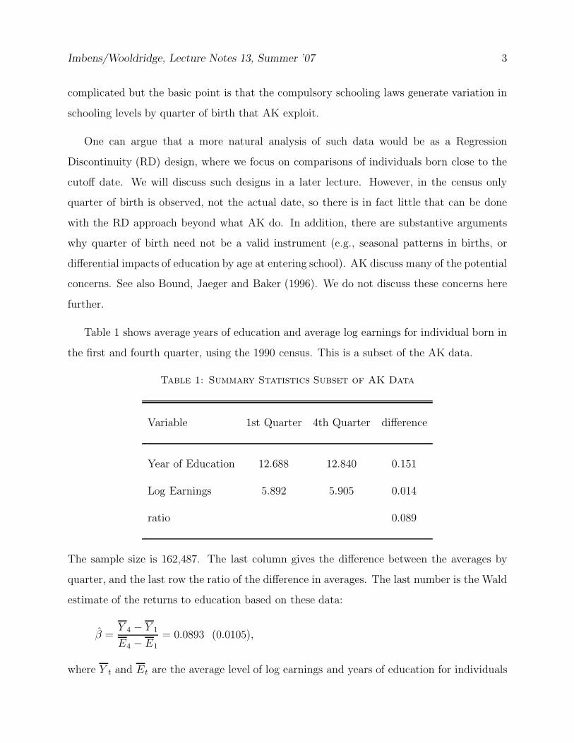
Imbens/Wooldridge, Lecture Notes 13, Summer ’07 3
complicated but the basic point is that the compulsory schooling laws generate variation in
schooling levels by quarter of birth that AK exploit.
One can argue that a more natural analysis of such data would be as a Regression
Discontinuity (RD) design, where we focus on comparisons of individuals born close to the
cutoff date. We will discuss such designs in a later lecture. However, in the census only
quarter of birth is observed, not the actual date, so there is in fact little that can be done
with the RD approach beyond what AK do. In addition, there are substantive arguments
why quarter of birth need not be a valid instrument (e.g., seasonal patterns in births, or
differential impacts of education by age at entering school). AK discuss many of the potential
concerns. See also Bound, Jaeger and Baker (1996). We do not discuss these concerns here
further.
Table 1 shows average years of education and average log earnings for individual born in
the first and fourth quarter, using the 1990 census. This is a subset of the AK data.
Table 1: Summary Statistics Subset of AK Data
Variable 1st Quarter 4th Quarter difference
Year of Education 12.688 12.840 0.151
Log Earnings 5.892 5.905 0.014
ratio 0.089
The sample size is 162,487. The last column gives the difference between the averages by
quarter, and the last row the ratio of the difference in averages. The last number is the Wald
estimate of the returns to education based on these data:
β =Y 4 − Y 1
E4 − E1
= 0.0893 (0.0105),
where Y t and Et are the average level of log earnings and years of education for individuals
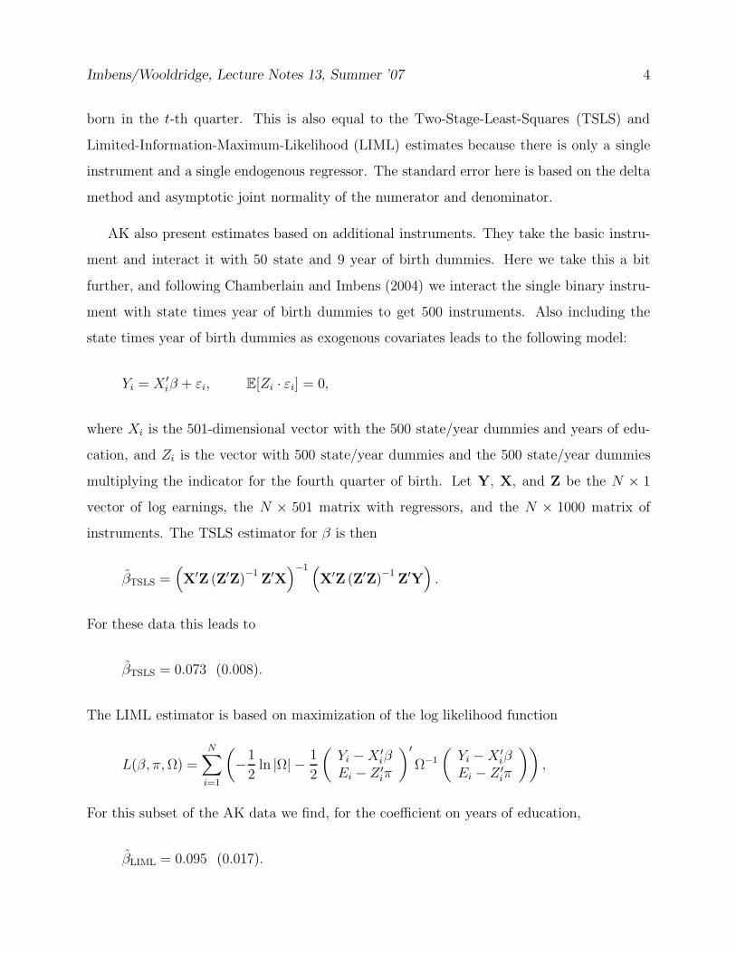
Imbens/Wooldridge, Lecture Notes 13, Summer ’07 4
born in the t-th quarter. This is also equal to the Two-Stage-Least-Squares (TSLS) and
Limited-Information-Maximum-Likelihood (LIML) estimates because there is only a single
instrument and a single endogenous regressor. The standard error here is based on the delta
method and asymptotic joint normality of the numerator and denominator.
AK also present estimates based on additional instruments. They take the basic instru-
ment and interact it with 50 state and 9 year of birth dummies. Here we take this a bit
further, and following Chamberlain and Imbens (2004) we interact the single binary instru-
ment with state times year of birth dummies to get 500 instruments. Also including the
state times year of birth dummies as exogenous covariates leads to the following model:
Yi = X ′iβ + εi, E[Zi · εi] = 0,
where Xi is the 501-dimensional vector with the 500 state/year dummies and years of edu-
cation, and Zi is the vector with 500 state/year dummies and the 500 state/year dummies
multiplying the indicator for the fourth quarter of birth. Let Y, X, and Z be the N × 1
vector of log earnings, the N × 501 matrix with regressors, and the N × 1000 matrix of
instruments. The TSLS estimator for β is then
βTSLS =(
X′Z (Z′Z)−1
Z′X)−1 (
X′Z (Z′Z)−1
Z′Y)
.
For these data this leads to
βTSLS = 0.073 (0.008).
The LIML estimator is based on maximization of the log likelihood function
L(β, π, Ω) =
N∑
i=1
(
−1
2ln |Ω| − 1
2
(
Yi − X ′iβ
Ei − Z ′iπ
)′
Ω−1
(
Yi − X ′iβ
Ei − Z ′iπ
))
,
For this subset of the AK data we find, for the coefficient on years of education,
βLIML = 0.095 (0.017).
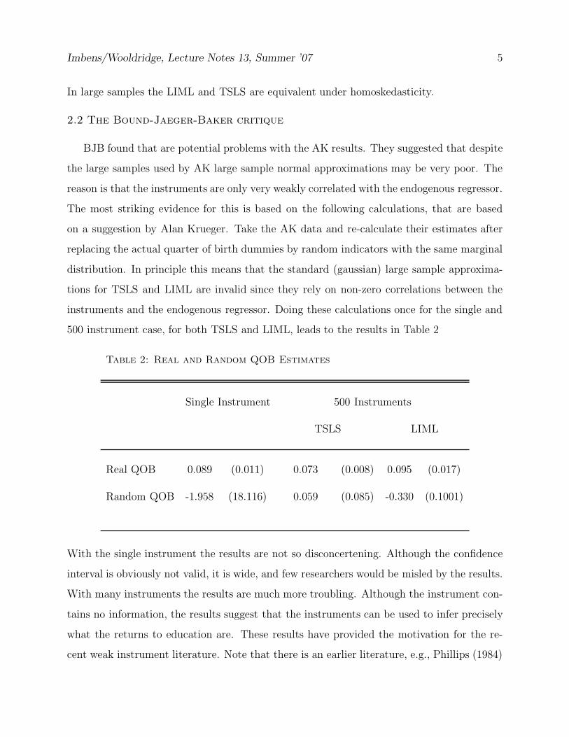
Imbens/Wooldridge, Lecture Notes 13, Summer ’07 5
In large samples the LIML and TSLS are equivalent under homoskedasticity.
2.2 The Bound-Jaeger-Baker critique
BJB found that are potential problems with the AK results. They suggested that despite
the large samples used by AK large sample normal approximations may be very poor. The
reason is that the instruments are only very weakly correlated with the endogenous regressor.
The most striking evidence for this is based on the following calculations, that are based
on a suggestion by Alan Krueger. Take the AK data and re-calculate their estimates after
replacing the actual quarter of birth dummies by random indicators with the same marginal
distribution. In principle this means that the standard (gaussian) large sample approxima-
tions for TSLS and LIML are invalid since they rely on non-zero correlations between the
instruments and the endogenous regressor. Doing these calculations once for the single and
500 instrument case, for both TSLS and LIML, leads to the results in Table 2
Table 2: Real and Random QOB Estimates
Single Instrument 500 Instruments
TSLS LIML
Real QOB 0.089 (0.011) 0.073 (0.008) 0.095 (0.017)
Random QOB -1.958 (18.116) 0.059 (0.085) -0.330 (0.1001)
With the single instrument the results are not so disconcertening. Although the confidence
interval is obviously not valid, it is wide, and few researchers would be misled by the results.
With many instruments the results are much more troubling. Although the instrument con-
tains no information, the results suggest that the instruments can be used to infer precisely
what the returns to education are. These results have provided the motivation for the re-
cent weak instrument literature. Note that there is an earlier literature, e.g., Phillips (1984)
Imbens/Wooldridge, Lecture Notes 13, Summer ’07 6
Rothenberg (1984), but it is the BJB findings that got the attention of researchers doing
empirical work.
2.3 Simulations with Weak Instruments and Varying Degrees of Endogeneity
Here we provide slightly more systematic simulation evidence of the weak instrument
problems in the AK setting. We create 10,000 artificial data sets, all of size 160,000, designed
to mimic the key features of the AK data. In each of these data sets half the units have
quarter of birth (denoted by Qi) equal to 0 and 1 respectively. Then we draw the two reduced
form residuals νi and ηi from a joint normal distribution
(
νi
ηi
)
∼ N((
00
)
,
(
0.446 ρ ·√
0.446 ·√
10.071
ρ ·√
0.446 ·√
10.071 10.071
))
.
The variances of the reduced form errors mimic those in the AK data. The correlation
between the reduced form residuals in the AK data is 0.318. The implied OLS coefficient is
ρ ·√
0.446/√
10.071. Then years of education is equal to
Ei = 12.688 + 0.151 · Qi + ηi,
and log earnings is equal to
Yi = 5.892 + 0.014 · Qi + νi.
Now we calculate the IV estimator and its standard error, using either the actual qob
variable or a random qob variable as the instrument. We are interested in the size of tests
of the null that coefficient on years of education is equal to 0.089 = 0.014/0.151. We base
the test on the t-statistic. Thus we reject the null if the ratio of the point estimate minus
0.089 and the standard error is greater than 1.96 in absolute value. We repeat this for 12
different values of the reduced form error correlation. In Table 3 we report the proportion
of rejections and the median and 0.10 quantile of the width of the estimated 95% confidence
intervals.
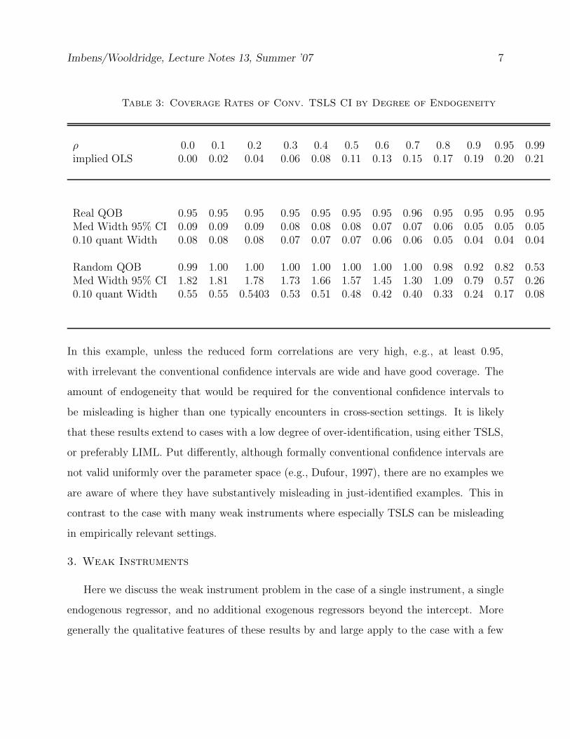
Imbens/Wooldridge, Lecture Notes 13, Summer ’07 7
Table 3: Coverage Rates of Conv. TSLS CI by Degree of Endogeneity
ρ 0.0 0.1 0.2 0.3 0.4 0.5 0.6 0.7 0.8 0.9 0.95 0.99implied OLS 0.00 0.02 0.04 0.06 0.08 0.11 0.13 0.15 0.17 0.19 0.20 0.21
Real QOB 0.95 0.95 0.95 0.95 0.95 0.95 0.95 0.96 0.95 0.95 0.95 0.95Med Width 95% CI 0.09 0.09 0.09 0.08 0.08 0.08 0.07 0.07 0.06 0.05 0.05 0.050.10 quant Width 0.08 0.08 0.08 0.07 0.07 0.07 0.06 0.06 0.05 0.04 0.04 0.04
Random QOB 0.99 1.00 1.00 1.00 1.00 1.00 1.00 1.00 0.98 0.92 0.82 0.53Med Width 95% CI 1.82 1.81 1.78 1.73 1.66 1.57 1.45 1.30 1.09 0.79 0.57 0.260.10 quant Width 0.55 0.55 0.5403 0.53 0.51 0.48 0.42 0.40 0.33 0.24 0.17 0.08
In this example, unless the reduced form correlations are very high, e.g., at least 0.95,
with irrelevant the conventional confidence intervals are wide and have good coverage. The
amount of endogeneity that would be required for the conventional confidence intervals to
be misleading is higher than one typically encounters in cross-section settings. It is likely
that these results extend to cases with a low degree of over-identification, using either TSLS,
or preferably LIML. Put differently, although formally conventional confidence intervals are
not valid uniformly over the parameter space (e.g., Dufour, 1997), there are no examples we
are aware of where they have substantively misleading in just-identified examples. This in
contrast to the case with many weak instruments where especially TSLS can be misleading
in empirically relevant settings.
3. Weak Instruments
Here we discuss the weak instrument problem in the case of a single instrument, a single
endogenous regressor, and no additional exogenous regressors beyond the intercept. More
generally the qualitative features of these results by and large apply to the case with a few

Imbens/Wooldridge, Lecture Notes 13, Summer ’07 8
weak instruments. We consider the model
Yi = β0 + β1 ·Xi + εi,
Xi = π0 + π1 · Zi + ηi,
with (εi, ηi) ⊥⊥ Zi, and jointly normal with covariance matrix Σ. (The normality is mainly
for some of the exact results, and it does not play an important role.) The reduced form for
the first equation is
Yi = α0 + α1 · Zi + νi,
where the parameter of interest is β1 = α1/π1. Let
Ω = E
[(
νi
ηi
)
·(
νi
ηi
)′]
, and Σ = E
[(
εi
ηi
)
·(
εi
ηi
)′]
,
be the covariance matrix of the reduced form and stuctural disturbances respectively. Many
of the formal results in the literature are for the case of known Ω, and normal disturbances.
This is largely innocuous, as Ω can be precisely estimated in typical data sets. Note that
this it not the same as assuming that Σ is known, which is not innocuous since it depends
on Ω and β, and cannot be precisely estimated in settings with weak instruments
Σ =
(
Ω11 − 2βΩ12 + β2Ω22 Ω12 − βΩ22
Ω12 − βΩ22 Ω22
)
.
The standard estimator for β1 is
βIV
1 =1
N
∑N
i=1
(
Yi − Y) (
Zi − Z)
1
N
∑N
i=1
(
Xi − X) (
Zi − Z) ,
where Y =∑
i Yi/N , and similarly for X and Z.
Imbens/Wooldridge, Lecture Notes 13, Summer ’07 9
A simple interpretation of the weak instrument is that with the concentration parameter
λ = π2
1 ·N∑
i=1
(
Zi − Z)2/
σ2
η.
close to zero, both the covariance in the numerator and the covariance in the denomina-
tor are close to zero. In reasonably large samples both are well approximated by normal
distributions:
√N
(
1
N
N∑
i=1
(
Yi − Y) (
Zi − Z)
−Cov(Yi, Zi)
)
≈ N (0, V (Yi · Zi)) ,
and
√N
(
1
N
N∑
i=1
(
Xi − X) (
Zi − Z)
− Cov(Xi, ZI)
)
≈ N (0, V (Xi · Zi)) .
These two normal approximations tend to be accurate in applications with reasonable sample
sizes, irrespective of the population values of the covariances. If π1 6= 0, as the sample size
gets large, then the ratio will eventually be well approximated by a normal distribution
as well. However, if Cov(Xi, Zi) ≈ 0, the ratio may be better approximated by a Cauchy
distribution, as the ratio of two normals centered close to zero.
The weak instrument literature is concerned with inference for β1 when the concentration
parameter λ is too close to zero for the normal approximation to the ratio to be accurate.
Staiger and Stock (1997, SS) formalize the problem by investigating the distribution of
the standard IV estimator under an alternative asymptotic approximation. The standard
asymptotics (strong instrument asymptotics in the SS terminology) is based on fixed param-
eters and the sample size getting large. In their alternative asymptotic sequence SS model π1
as a function of the sample size, π1N = c/√
N , so that the concentration parameter converges
to a constant:
λ −→ c2 · V (Zi).
Imbens/Wooldridge, Lecture Notes 13, Summer ’07 10
SS then compare coverage properties of various confidence intervals under this (weak instru-
ment) asymptotic sequence.
The importance of the SS approach is not in the specific sequence. The concern is more
that if a particular confidence interval does not have the appropriate coverage asymptotically
under the SS asymptotics, then there are values of the (nuisance) parameters in a potentially
important part of the parameter space (namely around πi = 0) such that the actual coverage
is substantially away from the nominal coverage for any sample size. More recently the issue
has therefore been reformulated as requiring confidence intervals to have asymptotically the
correct coverage probabilities uniformly in the parameter space. See for a discussion from
this perspective Mikusheva (2007). For estimation this perspective is not helpful: there
cannot be estimators that are consistent for β∗ uniformly in the parameter space since if
π1 = 0, there are no consistent estimators for β1. However, for testing there are generally
confidence intervals that are uniformly valid, but they are not of the conventional form, that
is, a point estimate plus or minus a constant times a standard error.
3.1 Tests and Confidence Intervals in the Just-identified Case
Let the instrument Zi = Zi − Z be measured in deviations from its mean. Then define
the statistic
S(β1) =1
N
N∑
i=1
Zi · (Yi − β1 · Xi) .
Then, under the null hypothesis that β1 = β∗1, and conditional on the instruments, the
statistic√
N · S(β∗1) has an exact normal distribution
√N · S(β∗
1) ∼ N(
0,N∑
i=1
Z2
i · σ2
ε
)
.
Importantly, this result does not depend on the strength of the instrument. Anderson and
Rubin (1949, AR) propose basing tests for the null hypothesis
H0 : β1 = β0
1 , against the alternative hypothesis Ha : β1 6= β0
1 ,
Imbens/Wooldridge, Lecture Notes 13, Summer ’07 11
on this idea, through the statistic
AR(
β0
1
)
=N · S(β0
1)2
∑N
i=1Z2
i
·(
(
1 −β01
)
Ω
(
1−β0
1
))−1
.
This statistic has an exact chi-squared distribution with degrees of freedom equal to one. In
practice, of course, one does not know the reduced form covariance matrix Ω, but substituting
an estimated version of this matrix based on the average of the estimated reduced form
residuals does not affect the large sample properties of the test.
A confidence interval can be based on this test statistic by inverting it. For example, for
a 95% confidence interval for β1, we would get
CIβ10.95
= β1 |AR(β1) ≤ 3.84 .
Note that this AR confidence interval cannot be empty, because at the standard IV estimator
βIV1
we have AR(βIV1
) = 0, and thus βIV1
is always in the confidence interval. The confidence
interval can be equal to the entire real line, if the correlation between the endogenous re-
gressor and the instrument is close to zero. This is not surprising: in order to be valid even
if π1 = 0, the confidence interval must include all real values with probability 0.95.
3.3 Tests and Confidence Intervals in the Over-identified Case
The second case of interest is that with a single endogenous regressor and multiple in-
struments. We deal separately with the case where there are many (similar) instrument,
so this really concerns the case where the instruments are qualitatively different. Let the
number of instrumens be equal to K, so that the reduced form is
Xi = π0 + π′1Zi + ηi,
with Zi a k-dimensional column vector. There is still only a single endogenous regressor,
and no exogenous regressors beyond the intercept. All the results generalize to the case with
additional exogenous covariates at the expense of additional notatio. The AR approach can
Imbens/Wooldridge, Lecture Notes 13, Summer ’07 12
be extended easily to this over-identified case, because the statistic√
N · S(β∗1) still has a
normal distribution, but now a multivariate normal distribution. Hence one can base tests
on the AR statistic
AR(
β0
1
)
= N · S(
β0
1
)′
(
N∑
i=1
Zi · Z ′i
)−1
S(
β0
1
)
·(
(
1 −β01
)
Ω
(
1−β0
1
))−1
.
Under the same conditions as before this has an exact chi-squared distribution with degrees
of freedom equal to the number of instruments, k. A practical problem arises if we wish
to construct confidence intervals based on this statistic. Suppose we construct a confidence
interval, analogously to the just-identified case, as
CIβ10.95 =
β1
∣
∣AR(β1) ≤ X 2
0.95(K)
,
where X 20.95(k) is the 0.95 quantile of the chi-squared distribution with degrees of freedom
equal to k. The problem is that this confidence interval can be empty. The interpretation
is that the test does not only test whether β1 = β01, but also tests whether the instruments
are valid. However, one generally may not want to combine those hypotheses.
Kleibergen (2002) modifies the AR statistic and confidence interval construction. Instead
of the statistic S(β1), he considers a statistic that looks at the correlation between a particular
linear combination of the instruments (namely the estimated endogenous regressor) and the
residual:
S(
β0
1
)
=1
N
N∑
i=1
(
Z ′iπ1(β
0
1))
·(
Yi − β0
1 · Xi
)
,
where π is the maximum likelihood estimator for π1 under the restriction β1 = β01 . The test
is then based on the statistic
K(
β0
1
)
=N · S(β0
1)2
∑N
i=1Z2
i
·(
(
1 −β01
)
Ω
(
1−β0
1
))−1
.
Imbens/Wooldridge, Lecture Notes 13, Summer ’07 13
This statistic has no longer an exact chi-squared distribution, but in large samples it still
has an approximate chi-square distribution with degrees of freedom equal to one. Hence the
test is straightforward to implement using standard methods.
Moreira (2003) proposes a method for adjusting the critical values that applies to a
number of tests, including the Kleibergen test. His idea is to focus on similar tests, test
that have the same rejection probability for all values of the nuisance parameter. The
nuisance parameter is here the vector of reduced form coefficients π, since we assume the
residual covariance matrix is known. The way to adjust the critical values is to consider the
distribution of a statistic such as the Kleibergen statistic conditional on a complete sufficient
statistic for the nuisance parameter. In this setting a complete sufficient statistic is readily
available in the form of the maximum likelihood estimator under the null, π1(β01). Moreira’s
preferred test is based on the likelihood ratio. Let
LR(
β0
1
)
= 2 ·(
L(
β1, π)
− L(
β0
1 , π(β0
1))
)
,
be the likelihood ratio. Then let cLR(p, 0.95), be the 0.95 quantile of the distribution of
LR(β01) under the null hypothesis, conditional on π(β0
1) = p. The proposed test is to reject
the null hypothesis at the 5% level if
LR(
β0
1
)
> cLR(π(β0
1), 0.95),
where conventional test would use critical values from a chi-squared distribution with a
single degree of freedom. This test can then be converted to construct a 95% confidence
intervals. Calculation of the (large sample) critical values is simplified by the fact that they
only depend on the number of instruments k, and a scaled version of the π(β01). Tabulations
of these critical values are in Moreira (2003) and have been programmed in STATA (See
Moreira’s website).
3.4 Conditioning on the First Stage
The AR, Kleibergen and Moreira proposals for confidence intervals are asymptotically
Imbens/Wooldridge, Lecture Notes 13, Summer ’07 14
valid irrespective of the strength of the first stage (the value of π1). However, they are not
valid if one first inspects the first stage, and conditional on the strength of that, decides to
proceed. Specifically, if in practice one first inspects the first stage, and decide to abandon
the project if the first stage F-statistic is less than some fixed value, and otherwise proceed
by calculating an AR, Kleibergen or Moreira confidence interval, the large sample coverage
probabilities would not necessarily be the nominal ones. In practice researchers do tend
to inspect and report the strength of the first stage. This is particularly true in recent
instrumental variables literature where researchers argue extensively for the validity of the
instrumental variables assumption. This typically involves detailed arguments supporting
the alleged mechanism that leads to the correlation between the endogenous regressor and the
instruments. For example, Section I in AK (page 981-994) is entirely devoted to discussing
the reasons and evidence for the relation between their instruments (quarter of birth) and
years of education. In such cases inference conditional on this may be more appropriate.
Chioda and Jansson (2006) propose a clever alternative way to construct a confidence
interval that is valid conditional on the strength of the first stage. Their proposed confidence
interval is based on inverting a test statistic similar to the AR statistic. It has a non-standard
distribution conditional on the strength of the first stage, and they suggest a procedure that
involves numerically approximating the critical values. A caveat is that because the first
stage F-statistic, or the first stage estimates are not ancillary, conditioning on them involves
loss of information, and as a result the Chioda-Jansson confidence intervals are wider than
confidence intervals that are not valid conditional on the first stage.
4. Many Weak Instruments
In this section we discuss the case with many weak instruments. The problem is both
the bias in the standard estimators, and the misleadingly small standard errors based on
conventional procedures, leading to poor coverage rates for standard confidence intervals in
many situations. The earlier simulations showed that especially TSLS, and to a much lesser
extent LIML, have poor properties in this case. Note first that resampling methods such as
bootstrapping do not solve these problems. In fact, if one uses the standard bootstrap with

Imbens/Wooldridge, Lecture Notes 13, Summer ’07 15
TSLS in the AK data, one finds that the average of the bootstrap estimates is very close to
the TSLS point estimat, and that the bootstrap variance is very close to the TSLS variance.
The literature has taken a number of approaches. Part of the literature has focused on
alternative confidence intervals analogues to the single instrument case. In addition a variety
of new point estimators have been proposed.
4.1 Bekker Asymptotics
In this setting alternative asymptotic approximations play a bigger role than in the single
instrument case. In an important paper Bekker (1995) derives large sample approximations
for TSLS and LIML based on sequences where the number of instruments increases propor-
tionally to the sample size. He shows that TSLS is not consistent in that case. LIML is
consistent, but the conventional LIML standard errors are not valid. Bekker then provides
LIML standard errors that are valid under this asymptotic sequence. Even with relatively
small numbers of instruments the differences between the Bekker and conventional asymp-
totics can be substantial. See also Chao and Swanson (2005) for extensions.
For the simple case with a single endogenous regressor, and no exogenous regressors
beyond the intercept, the adjustment to the variance is multiplicative. Thus, one can simply
multiply the standard LIML variance by
1 +K/N
1 − K/N·(
∑
i=1
(
π′1Zi
)2/
N
)−1
·((
1β1
)′
Ω−1
(
1β1
))−1
.
Substituting estimated values for the unknown parameters is likely to work fairly well in
practice. One can see from this expression why the adjustment can be substantial even
if K is small. The second factor can be large if the instruments are weak, and the third
factor can be large if the degree of endogeneity is high. If the instruments are strong, then∑
i=1(π′
1Zi)2/K will diverge, and the adjustment factor will converge to one.
4.2 Random Effects Estimators
Chamberlain and Imbens (2004, CI) propose a random effects quasi maximum likelihood
Imbens/Wooldridge, Lecture Notes 13, Summer ’07 16
estimator. They propose modelling the first stage coefficients πk, for k = 1, . . . , K, in the
regression
Xi = π0 + π′1Zi + ηi = π0 +
K∑
k=1
πk · Zik + ηi,
(after normalizing the instruments to have mean zero and unit variance,) as independent
draws from a normal N (µπ, σ2π) distribution. (More generally CI allow for the possibility that
only some of the first stage coefficients come from this common distribution, to take account
of settings where some of the instruments are qualitatively different from the others.) The
idea is partly that in most cases with many instruments, as for example in the AK study, the
instruments arise from interacting a small set of distinct instruments with other covariates.
Hence it may be natural to think of the coefficients on these instruments in the reduced
form as exchangeable. This notion is captured by modelling the first stage coefficients as
independent draws from the same distribution. In addition, this set up parametrizes the
many-weak instrument problem in terms of a few parameters: the concern is that the values
of both µπ and σ2π are close to zero.
Assuming also joint normality for (εi, ηi), one can derive the likelihood function
L(β0, β1, π0, µπ, σ2
π, Ω).
In contrast to the likelihood function in terms of the original parameters (β0, β1, π0, π1, Ω),
this likelihood function depends on a small set of parameters, and a quadratic approximation
to its logarithms is more likely to be accurate.
CI discuss some connections between the REQML estimator and LIML and TSLS in
the context of this parametric set up. First they show that in large samples, with a large
number of instruments, the TSLS estimator corresponds to the restricted maximum likeli-
hood estimator where the variance of the first stage coefficients is fixed at a large number,
or σ2π = ∞:
βTSLS ≈ arg maxβ0,β1,π0,µπ
= L(β0, β1, π0, µπ, σ2
π = ∞, Ω).
Imbens/Wooldridge, Lecture Notes 13, Summer ’07 17
From a Bayesian perspective, TSLS corresponds approximately to the posterior mode given
a flat prior on all the parameters, and thus puts a large amount of prior mass on values of
the parameter space where the instruments are jointly powerful.
In the same setting with a large number of instruments, no exogenous covariates, and a
known reduced form covariance matrix, the LIML estimator corresponds approximately to
the REQML estimator where we fix σ2π · (1 β1)
′Ω−1(1 β1)′ at a large number. In the special
case where we fix µπ = 0 and the random effects specification applies to all isntruments, CI
show that the REQML estimator is identical to LIML. However, like the Bekker asymptotics,
the REQML calculations suggests that the standard LIML variance is too small: the variance
of the REQML estimator is approximately equal to the standard LIML variance times
1 + σ−2
π ·((
1β1
)′
Ω−1
(
1β1
))−1
.
This is similar to the Bekker adjustment if we replace σ2π by
∑
i=1(π′
1Zi)2(K · N) (keeping
in mind that the instruments have been normalized to have unit variance). In practice the
CI adjustment will be bigger than the Bekker adjustment because the ml estimator for σ2π
will take into account noise in the estimates of the π, and so σ2π <
∑
i=1(π′
1Zi)2(K · N).
4.3 Choosing Subsets of the Instruments
In an interesting paper Donald and Newey (2001) consider the problem of choosing a
subset of an infinite sequence of instruments. They assume the instruments are ordered,
so that the choice is the number of instruments to use. Given the set of instruments they
consider a variety of estimators including TSLS and LIML. The criterion they focus on
is based on an approximation to the expected squared error. This criterion is not feasible
because it depends on unknown parameters, but they show that using an estimated version of
this leads to approximately the same expected squared error as using the infeasible criterion.
Although in its current form not straightforward to implement, this is a very promising
approach that can apply to many related problems such as generalized method of moments
settings with many moments.

Imbens/Wooldridge, Lecture Notes 13, Summer ’07 18
4.4 Other Estimators
Other estimators have also been investigated in the many weak instrument settings.
Hansen, Hausman and Newey (2006), and Hausman, Newey and Woutersen (2007) look at
Fuller’s estimator, which is modification of LIML that has finite moments. Phillips and Hale
(1977) (and later Angrist, Imbens and Krueger, 1999) suggest a jackknive estimator. Hahn,
Hausman and Kuersteiner (2004) look at jackknife versions of TSLS.
4.5 Flores’ simulations
Many simulations exercises have been carried out for evaluating the performance of testing
procedures and point estimators. In general it is difficult to assess the evidence of these
experiments. They are rarely tied to actual data sets, and so the choices for parameters,
distributions, sample sizes, and number of instruments are typically arbitrary.
In one of the more extensive simulation studies Flores-Lagunes (2007) reports results
comparing TSLS, LIML, Fuller, Bias corrected versions of TSLS, LIML and Fuller, a Jack-
nife version of TSLS (Hahn, Hausman and Kuersteiner, 2004), and the REQML estimator, in
settings with 100 and 500 observations, and 5 and 30 instruments for the single endogenous
variable. He looks at median bias, median absolute error, inter decile range, coverage rates,
and He concludes that “our evidence indicates that the random-effects quasi-maximum like-
lihood estimator outperforms alternative estimators in terms of median point estimates and
coverage rates.”
Imbens/Wooldridge, Lecture Notes 13, Summer ’07 19
References
Anderson, T., and H. Rubin, (1949), “Estimators of the Parameters of a Single
Equation in a Complete Set of Stochastic Equations,” Annals of Mathematical Statistics 21,
570-582-.
Andrews, D., M. Moreira, and J. Stock, (2006), “Optimal Two-sided Invariant
Similar Tests for Instrumental Variables Regresion,” Econometrica 74, 715-752-.
Andrews, D., and J. Stock, (2007), “Inference with Weak Instruments,” Advances
in Economics and Econometrics, Vol III, Blundel,, Newey and Persson (eds.), 122-173.
Angrist, J., G. Imbens, and A. Krueger, (1999), “Jackknife Instrumental Variables
Estimation,” Journal of Applied Econometrics, 14, 57-67.
Angrist, J., and A. Krueger, (1991), “Does Compulsory Schooling Attendance
Affect Schooling and Earnings,” Quarterly Journal of Economics 106, 979-1014.
Bekker, P., (1994), “Alternative Approximations to the Distribution of Instrumental
Variables Estimators,” Econometrica 62, 657-681.
Bound, J., A. Jaeger, and R. Baker, (1996), “Problems with Instrumental Vari-
ables Estimation When the Correlation Between the Instruments and the Endogenous Ex-
planatory Variable is Weak,” Journal of the American Statistical Association 90, 443-450.
Card, D., (2001), “Estimating the Return to Schooling: Progress on Some Persistent
Econometric Problems,” Econometrica 69(5), 1127-1160.
Chamberlain, G., and G. Imbens, (2004), “Random Effects Estimators with Many
Instrumental Variables,” Econometrica 72(1), 295-306.
Chao, J., and N. Swanson, (2005), “Consistent Estimation with a Large Number of
Weak Instruments,” Econometrica 73(5), 1673-1692.
Dufour, J.-M., (1997), “Impossibility Theorems in Econometrics with Applications to
Structural and Dynamic Models,” Econometrica 65, 1365-1387.
Imbens/Wooldridge, Lecture Notes 13, Summer ’07 20
Chioda, L., and M. Janson, (1998), “Optimal Conditional Inference for Instrumental
Variables Regression,” unpublished manuscript, department of economics, UC Berkeley.
Donald, S., and W. Newey, (2001), “Choosing the Number of Instruments,” Econo-
metrica 69, 1161-1191.
Flores-Lagunes, A., (2007), “Finite Sample Evidence of IV Estimators Under Weak
Instruments,” Journal of Applied Econometrics, 22, 677-694.
Fuller, W., (1977), “Some Properties of a Modification of the Limited Information
Estimator,” Econometrica 45(), 939-954.
Griliches, Z., (1977), “Estimating the Returns to Schooling – Some Econometric Prob-
lems,” Econometrica 45(1), 1-22.
Hahn, J., and J. Hausman, (2003), “Weak Instruments: Diagnosis and Cures in
Empirical Ecnometrics,” American Economic Review, Papers and Proceedings 93, 118-115.
Hahn, J., J. Hausman, and G. Kuersteiner, (2004), “Estimation with Weak Instru-
ments: Accuracy of Higher Order Bias and MSE Approxmiations,” Econometrics Journal.
Hansen, C., J. Hausman, and W. Newey, (2006), “Estimation with Many Instru-
mental Variables,” Unpublished Manuscript, Department of Economics, MIT.
Hausman, J., W. Newey, and T. Woutersen, (2006), “IV Estimation with Het-
eroskedasticity and Many Instruments,” Unpublished Manuscript, MIT.
Kleibergen, F., (2002), “Pivotal Statistics for Testing Structural Parameters in In-
strumental Variables Regression,” Econometrica 70(5), 1781-1803.
Mikusheva, A., (2007), “Uniform Inferences in Econometrics,” Chapter 3, PhD Thesis,
Harvard University, Department of Economics.
Moreira, M., (2001), “Tests with Correct Size when Instruments can be Arbitrarily
Weak,” Unpublished Paper, Department of Economics, Harvard University.
Imbens/Wooldridge, Lecture Notes 13, Summer ’07 21
Moreira, M., (2003), “A Conditional Likelihood Ratio Test for Structural Models,”
Econometrica 71(4), 1027-1048.
Philips, P., (1984), “Exact Small Sample Theory in the Simultaneous Equations Model,”
Handbook of Econometrics, (Griliches and Intrilligator, eds), Vol 2, North Holland.
Phillips, G., and C. Hale, (1977), “The Bias of Instrumental Variables Estimators
of Simultaneous Equations Systems,” International Economic Review, 18, 219-228.
Rothenberg, T., (1984), “Approximating the Distributions of Econometric Estimators
and Test Statistics,” Handbook of Econometrics, (Griliches and Intrilligator, eds), Vol 2,
Amsterdam, North Holland.
Staiger, D., and J. Stock, (1997), “Instrumental Variables Regression with Weak
Instruments,” Econometrica 68, 1055-1096.
Imbens/Wooldridge, Lecture Notes 14, Summer ’07
What’s New in Econometrics? NBER, Summer 2007Lecture 14, Wednesday, August 1st, 3:15-4:15 pm
Quantile MethodsThese notes review quantile estimation in a variety of situations, including models with
endogenous explanatory variables – including endogenous treatment effects – and panel datamodels with unobserved heterogeneity. Recent work on interpreting quantile estimators whenthe quantile is misspecified is also covered.1. Reminders About Means, Medians, and Quantiles
Consider the standard linear model in a population, with intercept and K 1 slopes :
y x u. (1.1)
Assume Eu2 , so that the distribution of u is not too spread out. Given a large randomsample, when should we expect ordinary least squares, which solves
mina,b∑i1
N
yi − a − xib2, (1.2)
and least absolute deviations (LAD), which solves
mina,b∑i1
N
|yi − a − xib|, (1.3)
to provide similar parameter estimates? There are two important cases. If
Du|x is symmetric about zero (1.4)
then OLS and LAD both consistently estimate and . If
u is independent of x with Eu 0, (1.5)
where Eu 0 is the normalization that identifies , then OLS and LAD both consistentlyestimate the slopes, . If u has an asymmetric distribution, then Medu ≡ ≠ 0, and LAD
converges to because Medy|x x Medu|x x . Of course,
independence between u and x rules out heteroskedasticity in Varu|x.In many applications, neither (1.4) nor (1.5) is likely to be true. For example, y may be a
measure of wealth, in which case the error distribution is probably asymmetric and Varu|xnot constant. Therefore, it is important to remember that if Du|x is asymmetric and changeswith x, then we should not expect OLS and LAD to deliver similar estimates of , even for“thin-tailed” distributions. In other words, it is important to separate discussions of resiliencyto outliers from the different quantities identified by least squares (the conditional mean,
1
Imbens/Wooldridge, Lecture Notes 14, Summer ’07
Ey|x) and least absolution deviations the conditional median, Medy|x. Of course, it is truethat LAD is much more resilient to changes in extreme values because, as a measure of centraltendency, the median is much less sensitive than the mean to changes in extreme values. But asignificant difference between OLS and LAD should not lead one to somehow prefer LAD. Itis possible that Ey|x x, Medy|x is not linear, and therefore LAD does notconsistently estimate . Generally, if we just use linear models as approximations to underlyingnonlinear functions, we should not be surprised if the linear approximation to the conditionalmean, and that for the median, can be very different. (Warning: Other so-called “robust”estimators, which are intended to be insensitive to outliers or influential data, usually requiresymmetry of the error distribution for consistent estimation. Thus, they are not “robust” in thesense of delivering consistency under a wide range of assumptions.)
Sometimes one can use a transformation to ensure conditional symmetry or theindependence assumption in (1.5). When yi 0, the most common transformation is thenatural log. Often, the linear model logy x u is more likely to satisfy symmetry orindependence. Suppose that symmetry about zero holds in the linear model for logy. Then,because the median passes through monotonic functions (unlike the expectation),Medy|x expMedlogy|x exp x, and so we can easily recover the partialeffects on the median of y itself. By contrast, we cannot generally findEy|x exp xEexpu|x. If, instead, we assume Du|x Du, then Medy|x andEy|x are both exponential functions of x, but with different “intercepts” inside theexponential function.
The fact that the median passes through monotonic functions is very handy for applyingLAD to a variety of problems, particularly corner solution responses where an outcome hasnonnegative support and a mass point at zero. But the expectation operator has usefulproperties that the median does not: linearity and the law of iterated expectations. To see howthese help to identify interesting quantities, suppose we begin with a random coefficient model
yi ai xibi, (1.6)
where ai is the heterogeneous intercept and bi is a 1 K matrix of heterogeneous slopes(“random coefficients”). If we assume that ai,bi is independent of xi, then
Eyi|xi Eai|xi xiEbi|xi ≡ xi, (1.7)
where Eai and Ebi. Because OLS consistently estimates the parameters of a
2
Imbens/Wooldridge, Lecture Notes 14, Summer ’07
conditional mean linear in those parameters, OLS consistently estimates the populationaveraged effects, or average partial effects, . Even under independence, there is no way toderive Medyi|xi without imposing more restrictions. In general, LAD of yi on 1,xi does notconsistently estimate or the medians of the elements of bij. Are there any reasonable
assumptions that imply LAD consistenty estimates something of interest in (1.7)? Yes,although multivariate symmetry is involved. With multivariate distributions there is no uniquedefinition of symmetry. A fairly strong restriction is the notion of a centrally symmetricdistribution (Serfling (2006)). If ui is a vector, then its distribution conditional on xi iscentrally symmetric if
Dui|xi D−ui|xi. (1.8)
This condition implies that, for any gi a function of xi, Dgi′ui|xi has a univariate distribution
that is symmetric about zero. Of course, (1.8) implies that Eui|xi 0.We can apply this to the random coefficient model as follows. Write ci ai,bi with
Ec i, and let di c i − . Then we can write
yi xi ai − xibi −
≡ xi gi′di
(1.9)
with gi 1,xi. Therefore, if c i has a centrally symmetric distribution about , then
Medgi′di|xi 0, and LAD applied to the usual model yi xi ui consistently estimates
and . Because ai and bi have centrally symmetric distributions about their and ,respectively, it is clear that these are the only sensible measures of central tendency in thedistribution of c i.
Usually, we are interested in how covariates affect quantiles other than the median, inwhich case quantile estimation is applied to a sequence of linear models. Write the th quantilein the distribution Dyi|xi as Quantyi|xi. Under linearity,
Quantyi|xi xi (1.10)
where, in general, the intercept and slopes depend on the quantile, . Under (1.10), consistentestimators of and are obtained by minimizing the asymmetric absolute loss functionor the “check” function:
min∈,∈K
∑i1
N
cyi − − xi, (1.11)
3
Imbens/Wooldridge, Lecture Notes 14, Summer ’07
where
cu 1u ≥ 0 1 − 1u 0|u| − 1u 0u (1.12)
and 1 is the “indicator function.” Consistency is relatively easy to establish because theobjective function is continuous in its parameters. Asymptotic normality is more difficultbecause any sensible definition of the Hessian of the objective function, away from thenondifferentiable kink, is identically zero. But it has been worked out under a variety ofconditions; see Koenker (2005) for a recent treatment.2. Some Useful Asymptotic Results2.1. What Happens if the Quantile Function is Misspecified?
When we use OLS to estimate the parameters of a linear model, we always have a simplecharacterization of the plim of the OLS estimator when the mean is not linear: If ∗ and ∗ arethe plims from the OLS regression yi on 1,xi then these provide the smallest mean squarederror approximation to Ey|x x. In other words, ∗,∗ solves
mina,b
Ex − − x2, (2.1)
where, of course, the expectation is over the distribution of x. Under some restrictions, (albeitrestrictive), j
∗ is the average partial effect Ex∂x/∂xj – multivariate normality of x is
sufficient – and under less restrictive (but still restrictive) assumptions, the j∗ estimate the
average partial effects up. These follow from the work of Chung and Goldberger (1984), Ruud(1984), and Stoker (1986).
Although the linear formulation of quantiles has been viewed by some – for example,Buchinsky (1991) and Chamberlain (1991) – as a linear approximation to the true conditionalquantile, most of the the linear model is treated as being correctly specified. In some ways, thisis strange because usually many quantiles are estimated. Yet assuming that different quantilesare linear in the same functions of x might be unrealistic.
Angrist, Chernozhukov, and Fernandez-Val (2006) provide a treatment of quantileregression under misspecification of the quantile function and characterize the probability limitof the LAD estimator. To describe the result, absorb the intercept into x and, rather thanassume a correctly specified conditional quantile, let be the solution to the populationquantile regression problem. Therefore, x is the plim of the estimated quantile function.ACF have a couple of different ways to characterize . One result is that solves
4
Imbens/Wooldridge, Lecture Notes 14, Summer ’07
min
Ewx,qx − x2, (2.2)
where the weight function wx, is
wx, 0
11 − ufy|xux 1 − uqx|xdu ≥ 0. (2.3)
In other words, is the best weighted mean square approximation to the true quantilefunction, where the weights are the average of the conditional density of yi over a line from thecandidate approximation, x, to the true quantile function, qx. The multiplication of thedensity by 1 − u gives more weight to points closer to the true conditional quantile. It isinteresting that the ACF characterization is in terms of a weighted mean squared error, aconcept we usually associate with conditional mean approximation. ACF also show anapproximation where the weighting function does not depend on , and use it characterize a“partial” regression quantiles, and to characterize omitted variables bias with quantileregression.2.2. Computing Standard Errors
First consider the case where we want to estimate the parameters in a linear quantile model,for a given quantile, . For a random draw, write
yi xi ui, Quantui|xi 0, (2.4)
where we include unity in xi so that contains an intercept and the slopes. Let be the quantileestimators, and define the quantile regression residuals, ûi yi − xi. Under weak conditions(see, for example, Koenker (2005)), N − is asymptotically normal with asymptoticvariance
A−1BA−1, (2.5)
where
A ≡ Efu0|xixi′xi (2.6)
and
B ≡ 1 − Exi′xi. (2.7)
Expression (2.5) is the now familiar standard “sandwich” form of asymptotic variances. It isfully robust in the sense that it is valid without further assumptions on Dui|xi. The matrix Bis simple to estimate as
5
Imbens/Wooldridge, Lecture Notes 14, Summer ’07
B 1 − N−1∑i1
N
xi′xi , (2.8)
where 0 1 is the chosen quantile. This estimator is consistent under the weakassumption of finite second moments for xi. The matrix A is harder to estimate because of thepresence of fu0|xi, and we do not have a parametrix model for the density of ui given xi. Butwe only have to estimate this conditional density at u 0, so we could use a nonparametricdensity estimator (based on the ûi. Powell (1986, 1991) proposed a simpler approach, whichleads to
 2NhN−1∑i1
N
1|ûi|≤ hNxi′xi, (2.9)
where hN 0 is a nonrandom sequence shrinking to zero as N → with N hN → . aresufficient for consistency. The second condition controls how quickly hN shrinks to zero. Forexample, hN aN−1/3 for any a 0 satisfies these conditions. The practical problem inchoosing a (or choosing hN more generally) is discussed by Koenker (2005), who alsodiscusses some related estimators. In particular, in equation (2.9), observation i does notcontribute if |ûi| hN. Other methods allow each observation to enter the sum but with a weightthat declines as |ûi| increases. (As an interesting aside, the derivation of (2.9) involves thesimple equality E1|ui|≤ hN|xixi
′xi E1|ui|≤ hNxi′xi, which is analogous to the key
step in the regression frameworks for justifying the heteroskedasticity-robust variance matrixestimator.)
The nonparametric bootstrap can be applied to quantile regression, but if the data set islarge, the computation using several hundred bootstrap samples can be costly.
If we assume that ui is independent of xi then fu0|xi fu0 and equation (2.5) simplifiesto
1 − fu02 Exi
′xi−1 (2.10)
and its estimator has the general form
1 − fu02
N−1∑i1
N
xi′xi
−1
, (2.11)
and a simple, consistent estimate of fu0 is the histogram estimator
6
Imbens/Wooldridge, Lecture Notes 14, Summer ’07
fu0 2NhN−1∑i1
N
1|ûi|≤ hN. (2.12)
Of course, one can use other kernel estimators for fu0. This nonrobust estimator is the onecommonly reported as the default be statistical packages, including Stata.
If the quantile function is misspecified, even the “robust” form of the variance matrix,based on the estimate in (2.9), is not valid. In the generalized linear models and generalizedestimating equations literature, the distinction is sometimes made between a “fully robust”variance estimator and a “semi-robust” variance estimator. In the GLM and GEE literatures,the semi-robust estimator assumes Eyi|xi, or the panel version of it, is correctly specified, butdoes not impose restrictions on Varyi|xi or other features of Dyi|xi. On the other hand, afully robust variance matrix estimator is consistent for the asymptotic variance even if themean function is misspecified. For, say, nonlinear least squares, or quasi-MLE in the linearexponential family, one needs to include the second derivative matrix of the conditional meanfunction to have a fully robust estimator. For some combinations of mean functions andobjective functions, the Hessian of the mean function disappears, and the fully robust andsemi-robust estimators are the same. For two-step methods, such as GEE, analytical formulasfor fully robust estimators are very difficult to obtain, and almost all applications use thesemi-robust form. This is a long-winded way to say that there is precedent for worrying abouthow to estimate asymptotic variances when the main feature being estimated is misspecified.
In GEE terminology, Â−1BÂ−1 where  is given by (2.9), is only semi-robust.Kim and White (2002) and Angrist, Chernozhukov, and Fernández-Val (2006) provide a
fully robust variance matrix estimator when the linear quantile function is possiblymisspecified. The estimator of A in (2.9) is still valid, but the estimator of B needs to beextended. If we use the outer product of the score we obtain
B N−1∑i1
N
− 1ûi 02xi′xi , (2.13)
where the ûi are the residuals from the (possibly) misspecified quantile regression, is generallyconsistent.
As shown by Hahn (1995, 1997), the nonparametric bootstrap (and the Bayesian bootstrap)generally provides consistent estimates of the fully robust variance without claims about theconditional mean being correct. It does not, however, provide asymptotic refinements for
7
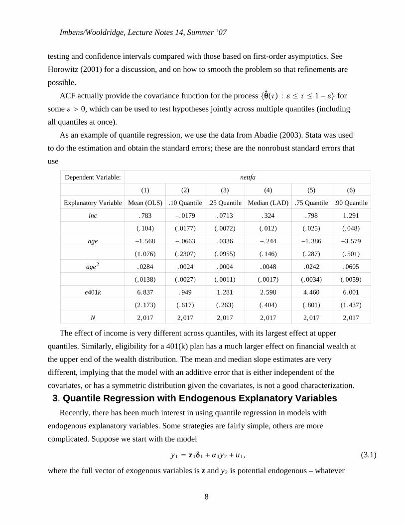
Imbens/Wooldridge, Lecture Notes 14, Summer ’07
testing and confidence intervals compared with those based on first-order asymptotics. SeeHorowitz (2001) for a discussion, and on how to smooth the problem so that refinements arepossible.
ACF actually provide the covariance function for the process : ≤ ≤ 1 − forsome 0, which can be used to test hypotheses jointly across multiple quantiles (includingall quantiles at once).
As an example of quantile regression, we use the data from Abadie (2003). Stata was usedto do the estimation and obtain the standard errors; these are the nonrobust standard errors thatuse
Dependent Variable: nettfa
(1) (2) (3) (4) (5) (6)
Explanatory Variable Mean (OLS) .10 Quantile .25 Quantile Median (LAD) .75 Quantile .90 Quantile
inc . 783 −. 0179 . 0713 . 324 . 798 1. 291
. 104 . 0177 . 0072 . 012 . 025 . 048
age −1. 568 −. 0663 . 0336 −. 244 −1. 386 −3. 579
1. 076 . 2307 . 0955 . 146 . 287 . 501
age2 . 0284 . 0024 . 0004 . 0048 . 0242 . 0605
. 0138 . 0027 . 0011 . 0017 . 0034 . 0059
e401k 6. 837 . 949 1. 281 2. 598 4. 460 6. 001
2. 173 . 617 . 263 . 404 . 801 1. 437
N 2, 017 2, 017 2, 017 2, 017 2, 017 2, 017
The effect of income is very different across quantiles, with its largest effect at upperquantiles. Similarly, eligibility for a 401(k) plan has a much larger effect on financial wealth atthe upper end of the wealth distribution. The mean and median slope estimates are verydifferent, implying that the model with an additive error that is either independent of thecovariates, or has a symmetric distribution given the covariates, is not a good characterization.3. Quantile Regression with Endogenous Explanatory Variables
Recently, there has been much interest in using quantile regression in models withendogenous explanatory variables. Some strategies are fairly simple, others are morecomplicated. Suppose we start with the model
y1 z11 1y2 u1, (3.1)
where the full vector of exogenous variables is z and y2 is potential endogenous – whatever
8
Imbens/Wooldridge, Lecture Notes 14, Summer ’07
that means in the context of quantile regression. The most straightforward case to handle isleast absolute deviations, because median restrictions are easier to justify when jointdistributions are involved.
Amemiya’s (1982) two-stage LAD estimator, whose asymptotic properties were derived byPowell (1986), adds a reduced form for y2, say
y2 z2 v2. (3.2)
While (3.2) can be estimated by OLS to obtain 2, using LAD in the first stage to estimate 2
is more in the spirit of 2SLAD. In the second step, the fitted values, ŷ i2 zi2, are inserted inplace of yi2 to given LAD of yi1 on zi1,ŷ i2. By replacing 2 with 2, it is clear that the 2SLADestimator essentially requires symmetry of the composite error 1v2 u1. While the propertiesof 2SLAD were originally worked out for nonstochastic zi – so that ui1,vi2 is independent ofzi – it is clear that symmetry of 1v2 u1 given z is sufficient.
We might as well assume Du1,v2|z is centrally symmetric, in which case a controlfunction approach can be used, too. Write
u1 1v2 e1, (3.3)
where e1 given z would have a symmetric distribution. Because Medv2|z 0, the first stageestimator can be LAD. Given the LAD residuals vi2 yi2 − zi2, these residuals can be addedto second-stage LAD. So, we do LAD of yi1 on zi1,yi2, vi2. It seems likely that a t test on vi2 isvalid as a test for the null that y2 is exogenous.
There can be problems of interpretation in just applying either 2SLAD or the CF approach.Suppose we view this as an omitted variable problem, where a1 is the omitted variable, andinterest lies in the “structual” median
Medy1|z,y2,a1 Medy1|z1,y2,a1 z11 1y2 a1. (3.4)
Then we can write
y1 z11 1y2 a1 e1
Mede1|z,y2,a1 0. (3.5) (3.6)
If (3.4) was stated in terms of means, then Ee1|z 0 by construction, and a very sensibleexogeneity condition is Ea1|z Ea1 0 (as a normalization) or that Covz,a1 0. Buthere we cannot even assert that Mede1|z Mede1 because (3.6) does not imply this; thereis no law of iterated medians. To further compound the problem, the median of the sum is notthe sum of the medians; so, even if we stated exogeneity as Meda1|z Meda1 and just
9
Imbens/Wooldridge, Lecture Notes 14, Summer ’07
asserted Mede1|z Mede1, a1 e1 u1 would not generally satisfyMedu1|z Medu1. Of course, we can make enough multivariate symmetric assumptions sothat all linear combinations of errors have symmetric distributions. But then LAD methods arepurely to guard against outliers; usual 2SLS will provide consisten, asymptotically normalestimates of the parameters under symmetry (and, of course, weaker assumptions).
With quantile estimation, such two-step estimators are even more difficult to justify. TheAngrist, Chernozhukov, and Fernandez-Val (2006) partialling out representations can providesome sort of interpretation of netting out the control, v2, but it is difficult to know whether theparameters are ultimately interesting.
Abadie (2003) and Abadie, Angrist, and Imbens (2002) show how to define and estimatepolicy parameters with a binary endogenous treatment, say D, and binary instrumentalvariable, say Z. The outcome is Y with observed covariates, X. The potential outcomes on Y areYd, d 0,1 – that is, without treatment and with treatment, respectively. The counterfactualsfor treatment are Dz, z 0,1. Thus, D0 is what treatment status would be if the instrument(often, randomized eligibility) equals zero, and D1 is treatment status if Z 1. The data weobserve are X,Z,D 1 − ZD0 ZD1, and Y 1 − DY0 DY1. As discussed in AAI,identification of average treatment effects, and ATE on the treated, is difficult. Instead, theyfocus on treatment effects for compliers, that is, the (unobserved) subpopulation withD1 D0. This is the group of subjects who do not participate if ineligible but do participate ifeligible.
AAI specify the linear equation
QuantY|X,D,D1 D0 D X, (3.7)
and define as the quantile treatment effect (QTE) for compliers. If we observed the eventD1 D0, then (3.7) could be estimated by standard quantile regression using the subsample ofcompliers. But, in effect, the binary variable 1D1 D0 is an omitted variable. But Z is anavailable instrument for D. As discussed by AAI, (3.7) identifies differences in quantiles onthe potential outcomes, Y1 and Y0, and not the quantile of the difference, Y1 − Y0. The lattereffects are harder to identify. (Of course, in the case of mean effects, there is no difference inthe two effects.)
The assumptions used by AAI to identify are
Y1,Y0,D1,D0 is independent of Z conditional on X (3.8)
10
Imbens/Wooldridge, Lecture Notes 14, Summer ’07
0 PZ 1|X 1 (3.9)
PD1 1|X ≠ PD0 1|X (3.10)
PD1 ≥ D0|X 1. (3.11)
Under these assumptions, AAI show that a weighted quantile estimation identifies . Theestimator that is computationally most convenient is obtained as follows. Define
vU 1 − D1 − vU1 − X − 1 − DvU
X , (3.12)
where U Y,D,X, vU PZ 1|U, and X PZ 1|X. AAI show thatu PD1 D0|U u, and so this weighting function is nonnegative. They also showthat and in (3.7) solve
min,
EUcY − D − X, (3.13)
where c is the check function defined earlier. To operationalize the estimate, needs tobe estimated, which means estimating PZ 1|Y,D,X and PZ 1|X. AAI use linear seriesestimators to approximate PZ 1|Y,D,X and PZ 1|X, and derive the asymptotic varianceof the two-step estimator that solves
min∑i1
N
1vUi ≥ 0vUicYi − Wi, (3.14)
where Wi Di,Xi and contains and . The indicator function 1vUi ≥ 0 ensures thatonly observations with nonnegative weights are used. Asymptotically, vu ≥ 0, and thistrimming of observations becomes less and less necessary. To ensure that vu and x actlike probabilities, series estimation using logit functions, as in Hirano, Imbens, and Ridder(2003), might be preferred (although that still would not ensure nonnegativity of vUi for alli).
Other recent work has looked at quantile estimation with endogenous treatment effects.Chernozhukov and Hansen (2005, 2006) consider indentification and estimation of QTEs in amodel with endogenous treatment and without imposing functional form restrictions. Letqd,x, denote the th quantile function for treatment level D d and covariates x. In thebinary case, CH define the QTE as
QTEx q1,x, − q0,x,. (3.15)
11
Imbens/Wooldridge, Lecture Notes 14, Summer ’07
Using a basic result from probability, the average treatment effect, again conditional on x, canbe obtained by integrating (3.15) over 0 1.
The critical representation used by CH is that each potential outcome, Yd, conditional onX x, can be expressed as
Yd qd,x,Ud (3.16)
where
Ud|Z ~Uniform0,1, (3.17)
and Z is the instrumental variable for treatment assignment, D. Thus, D is allowed to becorrelated with Ud. Key assumptions are that qd,x,u is strictly increasing in u and a “rankinvariance” condition. The simplest form of the condition is that , conditional on X x andZ z, Ud does not depend on d. The CH show that, with the observed Y defined asY qD,X,UD,
PY ≤ qD,X,|X,Z PY qD,X,|X,Z . (3.18)
Equation (3.18) acts as a nonparametric conditional moment condition which, under certainassumptions, allows identification of qd,x,. If we define R Y − qD,X,, then (3.18)implies that the th quantile of R, conditional on X,Z, is zero. This is similar to the morecommon situation where we have a conditional moment condition of the form ER|X,Z 0.See Chernozhukov and Hansen (2005) for details concerning identification – they apply resultsof Newey and Powell (2003) – and Chernozhukov and Hansen (2005) for estimation methods,where they assume a linear form for qd,x, and obtain what they call the quantile regressioninstrumental variables estimator.
Other work that uses monotonicity assumptions and identifies structural quantile functionsis Chesher (2003) and Imbens and Newey (2006).4. Quantile Regression for Panel Data
Quantile regression methods can be applied to panel data, too. For a given quantile0 1, suppose we specify
Quantyit|xit xit, t 1, . . . ,T, (4.1)
where xit probably allows for a full set of time period intercepts. Of course, we can writeyit xit uit where Quantuit|xit 0. The natural estimator of o is the pooled quantile
regression estimator. Unless we assume that (3.1) has correctly specified dynamics, thevariance matrix needs to be adjusted for serial correlation in the resulting score of the objective
12
Imbens/Wooldridge, Lecture Notes 14, Summer ’07
function. These scores have the form
sit −xit′ 1yit − xit ≥ 0 − 1 − 1yit − xit 0, (4.2)
which can be shown to have zero mean (at the “true” parameter), conditional on xit, under(4.1). The serial dependence properties are not restricted, nor is heterogeneity in thedistributions across t. A consistent estimator of B (with T fixed and N → ) is
B N−1∑i1
N
∑t1
T
∑r1
T
sitsir′. (4.3)
This estimator is not robust to misspecification of the conditional quantiles, but the extensionof Angrist, Chernozhukov, and Fernandez-Val (2006) should work in the pooled panel datacase as well..
Estimation of A is similar to the cross section case. A robust estimator, that does notassume independence between uit and xit, and allows the distribution of uit to change across t,is
 2NhN−1∑i1
N
∑t1
T
1|ûit|≤ hNxit′ xit, (4.4)
or, we can replace the indicator function with a smoothed version. Rather than using
Â−1BÂ−1/N as the estimate of the asymptotic variance of , the bootstrap can be applied byresampling cross section units.
Allowing explicitly for unobserved effects in quantile regression is trickier. For a givenquantile 0 1, a natural specification, which incorporates strict exogeneity conditional onci, is
Quantyit|xi,ci Quantyit|xit,ci xit ci, t 1, . . . ,T, (4.5)
which is reminiscent of the way we specified the conditional mean in Chapter 10.Equivalently, we can write
yit xit ci uit, Quantuit|xi,ci 0, t 1, . . . ,T. (4.6)
Unfortunately, unlike in the case of estimating effects on the conditional mean, we cannotproceed without further assumptions. A “fixed effects” approach, where we allow Dci|xi tobe unrestricted, is attractive. Generally, there are no simple transformations to eliminate ci andestimate . If we treat the ci as parameters to estimate along with , the resulting estimatorgenerally suffers from an incidental parameters problem. Briefly, if we try to estimate ci for
13
Imbens/Wooldridge, Lecture Notes 14, Summer ’07
each i then, with large N and small T, the poor quality of the estimates of ci causes theaccompanying estimate of to be badly behaved. Recall that this was not the case when weused the FE estimator for a conditional mean: treating the ci as parameters led us to the withinestimator. Koenker (2004) derives asymptotic properties of this estimation procedure when Tgrows along with N, but also adds the assumptions that the regressors are fixed anduit : t 1, . . . ,T is serially independent.
An alternative approach is suggested by Abrevaya and Dahl (2006) for T 2. They aremotivated by Chamberlain’s correlated random effects linear model. In the T 2 case,Chamberlain (1982) specifies
Eyt|x1,x2 t xt x11 x22, t 1,2. (4.7)
Notice that ∂Ey1|x/∂x1 1 and ∂Ey2|x/∂x1 1. Therefore,
∂Ey1|x∂x1
− ∂Ey2|x∂x1
, (4.8)
and similarly if we reverse the roles of x1 and x2. Abrevaya and Dahl use this motivation toestimate separate linear quantile regressions Quantyt|x1,x2 – reminiscent of Chamberlain’smethod – and then define the partial effect as
∂Quanty1|x
∂x1−∂Quanty2|x
∂x1. (4.9)
For quantile regression, CRE approaches are generically hampered because findingquantiles of sums of random variables is difficult. For example, suppose we impose theMundlak representation ci o xio ai. Then we can write
yit o xito xio ai uit ≡ yit o xito xio vit, where vit is the composite
error. Now, if we assume vit is independent of xi, then we can estimate o and o using pooled
quantile regression of yit on 1,xit, and xi. (The intercept does not estimate a quantity ofparticular interest.) But independence is very strong, and, if we truly believe it, then weprobably believe all quantile functions are parallel. Of course, we can always just assert thatthe effect of interest is the set of coefficients on xit in the pooled quantile estimation, and weallow these, along with the intercept and coefficients on xi, to change across quantile. Theasymptotic variance matrix estimator discussed for pooled quantile regression applies directlyonce we define the explanatory variables at time t to be 1,xit, xi.
We have more flexibility if we are interested in the median, and a few simple approachessuggest themselves. Write the model Medyit|xi,ci Medyit|xit,ci xit ci in error form
14
Imbens/Wooldridge, Lecture Notes 14, Summer ’07
as
yit xit ci uit, Meduit|xi,ci 0, t 1, . . ,T (4.10)
and consider the multivariate conditional distribution Dui|xi. Above we discussed thecentrally symmetric assumption, conditional on xi: Dui|xi D−ui|xi. If we make thisassumption, then the time-demeaned errors üit have (univariate) conditional (on xi
distributions symmetric about zero, which means we can consistently estimate by applyingpooled least absolute deviations to the time-demeaned equation ÿit xit üit, being sure toobtain fully robust standard errors for pooled LAD.
Alternatively, under the centrally symmetric assumption, the difference in the errors,Δuit uit − ui,t−1 have symmetric distributions about zero, so one can apply pooled LAD toΔyit Δxit Δuit, t 2, . . . ,T. From Honoré (1992) applied to the uncensored case, LAD onthe first differences is consistent when uit : t 1, . . . ,T is an i.i.d. sequence conditional onxi,ci, even if the common distribution is not symmetric – and this may afford robustness forLAD on the first differences rather than on the time-demeaned data. Interestingly, it followsfrom the discussion in Honoré (1992, Appendix 1) that when T 2, applying LAD on the firstdifferences is equivalent to estimating the ci along with o. So, in this case, there is noincidental parameters problem in estimating the ci as long as ui2 − ui1 has a symmetricdistribution. Although not an especially weak assumption, central symmetry of Dui|xi allowsfor serial dependence and heteroskedasticity in the uit (both of which can depend on xi or on t).As always, we should be cautious in comparing the pooled OLS and pooled LAD estimates of on the demeaned or differenced data because they are only expected to be similar under theconditional symmetry assumption.
If we impose the Mundlak-Chamberlain device, we can get by with conditional symmetryof a sequence of bivariate distributions. Write yit t xit xi ai uit, whereMeduit|xi,ai 0. If Dai,uit|xi has a symmetric distribution around zero then Dai uit|xi
is symmetric about zero, and, if this holds for each t, pooled LAD of yit on 1,xit, and xi
consistently estimates t,,. (Therefore, we can estimate the partial effects onMedyit|xit,ci and also test if ci is correlated with xi.) The assumptions used for this approachare not as weak as we would like, but, like using pooled LAD on the time-demeaned data,adding xi to pooled LAD gives a way to compare with the usual FE estimate of . .(Remember, if we use pooled OLS with xi included, we obtain the FE estimate.) Fully robust
inference can be obtained by computing B and  in (4.3) and (4.4).
15
Imbens/Wooldridge, Lecture Notes 14, Summer ’07
5. Quantile Methods for “Censored” DataAs is well known, the statistical structure of parametric models for data that have truly
been censored – such as top-coded wealth, or a right-censored duration – is essentially thesame as models for corner solution responses – that is, variables that have a mass point, or pileup, at one or couple of values (usually, zero). Examples are labor supply, charitablecontributions, and amount of life insurance. But an important point is that the interpretation ofthe estimates is different in these two cases. In the data censoring case, there is an underlyinglinear model (usually) whose coefficients we are interested in. For example, we are interestedin the conditional distribution of wealth given covariates. That wealth has been top-codedmeans that we do not observe underlying wealth over its entire range. In effect, it is a missingdata problem. The same is true with duration models.
In the corner solution case, we observe the response of interest over its entire range. Weuse models such as Tobit simply because we want to recognize the mass point or points. Linearfunctional forms for the mean, say, can miss important nonlinearities. When we apply, say,standard Tobit to a corner solution, y, we are interested in features of Dy|x, such asPy 0|x, Ey|x,y 0, and Ey|x. While the parameters in the model are important, they donot directly provide partial effects on the quantities of interest. Of course, if we use a linearmodel approximation for, say, Ey|x, then the coefficients are approximate partial effects. Arelated point is: if we modify standard models for corner responses, say, considerheteroskedasticity in the latent error of a Tobit, we should consider how it affects Dy|x, andnot just the paramter estimates. In the case of censored data, it is the parameters of theunderlying linear model we are interested in, and then it makes much more sense to focus onparameter sensitivity.
In applying LAD methods to “censored” outcomes, we should also be aware of thedifference between true data censoring and corner solution responses. With true data censoringwe clearly have an interest in obtaining estimates of, say,
yi∗ xi ui, (5.1)
where yi∗ is the variable we would like to explain. If yi
∗ is top coded at, say, ri, then we observeyi minyi
∗, ri. If we assume Dui|xi, ri Normal0,2, then we can apply censorednormal regression (also called type I Tobit). This method applies even if ri is observed onlywhen yi
∗ has been censored, which happens sometimes in duration studies. As shown byPowell (1986), we can estimate (5.1) under much weaker assumptions than normality:
16
Imbens/Wooldridge, Lecture Notes 14, Summer ’07
Medui|xi, ri 0 (5.2)
suffices, provided the censoring values value, ri, are always observed. Because the medianpasses through monotonic functions,
Medyi|xi, ri Medminxi ui, ri|xi, ri
minMedxi ui|xi, ri, ri
minxi, ri. (5.3)
Because LAD consistently estimates the parameters of a conditional median, at least undercertain regularity conditions, (5.3) suggest estimate as the solution to
minb∑i1
N
|yi − minxib, ri|. (5.4)
Powell (1986) showed that, even though the objective function has a corner it it, the censoredleast absolute deviations (CLAD) estimator is N -asymptotically normal. Honoré, Khan, andPowell (2002) provide methods that can be used when ri is not always observed.
CLAD can also be applied to corner solution responses. Suppose the variable of interest, yi,has a corner at zero, and is determined by
y max0,x u. (5.5)
If Du|x is Normal0,2, then the MLE is the type I Tobit. Given and 2, we can computepartial effects on the mean and various probabilities. The partial effects on Medy|x dependonly on , because
Medy|x max0,x. (5.6)
Of course, (5.6) provides a way to estimate by CLAD under just
Medu|x 0. (5.7)
The j measure the partial effects on Medy|x once Medy|x 0.
Once we recognize in corner solution applications that it is features of Dy|x that are ofinterest, (5.6) becomes just a particular feature of Dy|x that we can identify, and it is nobetter or worse than other features of Dy|x that we might want to estimate, such as a quantileother than the median, or the mean Ey|x, or the “conditional” mean, Ey|x,y 0. Emphasisis often given on the fact that the functional form for the median in (5.6) holds very generallywhen (5.5) holds; other than (5.7), no restrictions are made on the shape of the distributionDu|x or of its dependence on x. But for corner solution responses, there is nothing sacred
17
Imbens/Wooldridge, Lecture Notes 14, Summer ’07
about (5.5). In fact, it is pretty restrictive because y depends on only one unobservable, u.Two-part models, summarized recently in Wooldridge (2007), allow more flexibility.
A model that is no more or less restrictive than (5.5) is
y a expx, (5.8)
where the only assumption we make is
Ea|x 1, (5.9)
where Da|x is otherwise unrestricted. In particular, we do not know Pa 0|x, which ispositive if y has mass point at zero, or Meda|x. Under (5.9),
Ey|x expx, (5.10)
which means we can consistently estimate using nonlinear regression or a quasi-MLE in thelinear exponential family (such as Poisson or Gamma); it does not matter that y is a corner if itsmean is given by (5.10). The point here is that, if we simply focus on assumptions and whatcan be identified under those assumptions, the model in (5.8) and (5.9) identifies just as manyfeatures of Dy|x as the model in (5.5) and (5.7). They are different features, but neither isinherently better than the other.
Continuing with this point, we can modify (5.5) rather simply and see that CLAD breaksdown. Suppose we add multiplicative heterogeneity:
y a max0,x u, (5.11)
where a ≥ 0, and even make the strong assumption that a is independent of x,u. Thedistribution Dy|x now depends on the distribution of a, and does not follow a type I Tobitmodel; generally, finding its distribution would be difficult, even if we specify a simpledistribution for a. Nevertheless, if we normalize Ea 1, thenEy|x,u Ea|x,u max0,x u max0,x u (because Ea|x,u 1). It followsimmediately by iterated expectations that if assumption (17.3) holds, then Ey|x has exactlythe same form as the type I Tobit model:
Ey|x x/x x/. (5.12)
Therefore, the parameters and 2 are identified and could be estimate by nonlinear leastsquares or weighted NLS, or a quasi-MLE using the mean function (5.12). Note that Dy|xdoes not follow the type I Tobit distribution, so MLE is not available.
On the other hand, if we focus on the median, we have
18
Imbens/Wooldridge, Lecture Notes 14, Summer ’07
Medy|x,a a max0,x. (5.13)
But there is no “law of iterated median,” so, generaly, we cannot determine Medy|x withoutfurther assumptions. One might argue that we are still interested in the j because they
measure the average partial effects on the median. But the do not appear to be generallyidentified under this variation on the standard Tobit model.
The issues in applying CLAD to corners gets even trickier in panel data applications.Suppose
yit max0,xit ci uit
Meduit|xi,ci 0, (5.14) (5.15)
so that (5.15) embodies strict exogeneity of xit conditional on ci. Under (5.14) and (5.15),
Medyit|xi,ci max0,xit ci. (5.16)
Honoré (1992) and Honoré and Hu (2004) provide methods of estimating without making
any assumptions about the distribution of ci, or restricting its dependence on xi. They doassume conditional exchangeability assumptions on the uit; sufficient is independence with xi
and uit i.i.d. over t. Given estimates of the j, we can estimate the partial effects of the xtj on
Medyt|xt,c for Medyt|xt,c 0. Unfortunately, because we do not observe ci, or knowanything about its distribution, we do not know when the nonzero effect kicks in. We can writethe partial effect of xtj as
tjxt,c 1xt c 0j. (5.17)
We might be interested in averaging these across the distribution of unobserved heterogeneity,but this distribution is not identified. (Interesting, if ci has a Normalc,c
2 distribution, thenit is easy to show that the average of (5.17) across the heterogeneity isEci tjxt,ci c − xt/cj, and we can see immediatly that it depends on the
location and scale of ci.)We can compare the situation of the median with the mean. Using the Altonji and Matkin
(2005), suppose we assume Dci|xi Dci|xi. Then Eyit|xi gtxit, xi for someunknown function gt, , and is identified (usually only up to scale) and the average partialeffects on the mean are generally identified.References
(To be added.)
19
Imbens/Wooldridge, Lecture Notes 15, Summer ’07 1
What’s New in Econometrics NBER, Summer 2007
Lecture 15, Wednesday, Aug 1st, 4.30-5.30pm
Generalized Method of Moments and Empirical Likelihood
1. Introduction
Generalized Method of Moments (henceforth GMM) estimation has become an important
unifying framework for inference in econometrics in the last twenty years. It can be thought
of as nesting almost all the common estimation methods such as maximum likelihood, or-
dinary least squares, instrumental variables and two–stage–least–squares and nowadays it is
an important part of all advanced econometrics text books (Gallant, 1987; Davidson and
McKinnon, 1993; Hamilton, 1994; Hayashi, 2000; Mittelhammer, Judge, and Miller, 2000;
Ruud, 2000; Wooldridge, 2002). Its formalization by Hansen (1982) centers on the presence
of known functions, labelled “moment functions”, of observable random variables and un-
known parameters that have expectation zero when evaluated at the true parameter values.
The method generalizes the “standard” method of moments where expectations of known
functions of observable random variables are equal to known functions of the unknown pa-
rameters. The “standard” method of moments can thus be thought of as a special case of
the general method with the unknown parameters and observed random variables entering
additively separable. The GMM approach links nicely to economic theory where orthogonal-
ity conditions that can serve as such moment functions often arise from optimizing behavior
of agents. For example, if agents make rational predictions with squared error loss, their
prediction errors should be orthogonal to elements of the information set. In the GMM
framework the unknown parameters are estimated by setting the sample averages of these
moment functions, the “estimating equations,” as close to zero as possible.
The framework is sufficiently general to deal with the case where the number of moment
functions is equal to the number of unknown parameters, the so–called “just–identified case”,
as well as the case where the number of moments exceeding the number of parameters to be
estimated, the “over–identified case.” The latter has special importance in economics where
Imbens/Wooldridge, Lecture Notes 15, Summer ’07 2
the moment functions often come from the orthogonality of potentially many elements of
the information set and prediction errors. In the just-identified case it is typically possible
to estimate the parameter by setting the sample average of the moments exactly equal to
zero. In the over-identified case this is not feasible. The solution proposed by Hansen
(1982) for this case, following similar approaches in linear models such as two– and three–
stage–least–squares, is to set a linear combination of the sample average of the moment
functions equal to zero, with the dimension of the linear combination equal to the number
of unknown parameters. The optimal linear combination of the moments depends on the
unknown parameters, and Hansen suggested to employ initial, possibly inefficient, estimates
to estimate this optimal linear combination. Chamberlain (1987) showed that this class of
estimators achieves the semiparametric efficient bound given the set of moment restrictions.
The Chamberlain paper is not only important for its substantive efficiency result, but also
as a precursor to the subsequent empirical likelihood literature by the methods employed:
Chamberlain uses a discrete approximation to the joint distribution of all the variables to
show that the information matrix based variance bound for the discrete parametrization is
equal to the variance of the GMM estimator if the discrete approximation is fine enough.
Th empirical likelihood literature developed partly in response to criticisms regarding
the small sample properties of the two-step GMM estimator. Researchers found in a number
of studies that with the degree of over-identification high, these estimators had substantial
biases, and confidence intervals had poor coverage rates. See among others, Altonji and
Segal (1996), Burnside and Eichenbaum (1996) , and Pagan and Robertson (1997). These
findings are related to the results in the instrumental variables literature that with many or
weak instruments two-stage-least squares can perform very badly (e.g., Bekker, 1994; Bound,
Jaeger, and Baker, 1995; Staiger and Stock, 1997). Simulations, as well as theoretical results,
suggest that the new estimators have LIML-like properties and lead to improved large sample
properties, at the expense of some computational cost.
2. Examples
First the generic form of the GMM estimation problem in a cross–section context is

Imbens/Wooldridge, Lecture Notes 15, Summer ’07 3
presented. The parameter vector θ∗ is a K dimensional vector, an element of Θ, which is
a subset of RK . The random vector Z has dimension P , with its support Z a subset of
RP . The moment function, ψ : Z × Θ → RM , is a known vector valued function such that
E [ψ(Z, θ∗)] = 0, and E [ψ(Z, θ)] 6= 0 for all θ ∈ Θ with θ 6= θ∗. The researcher has available
an independent and identically distributed random sample Z1, Z2, . . . , ZN . We are interested
in the properties of estimators for θ∗ in large samples.
Many, if not most models considered in econometrics fit this framework. Below are some
examples, but this list is by no means exhaustive.
I. Maximum Likelihood
If one specifies the conditional distribution of a variable Y given another variable X as
fY |X(y|x, θ), the score function satisfies these conditions for the moment function:
ψ(Y,X, θ) =∂ ln f
∂θ(Y |X, θ).
By standard likelihood theory the score function has expectation zero only at the true value
of the parameter. Interpreting maximum likelihood estimators as generalized method of
moments estimators suggests a way of deriving the covariance matrix under misspecification
(e.g., White, 1982), as well as an interpretation of the estimand in that case.
II. Linear Instrumental Variables
Suppose one has a linear model
Y = X ′θ∗ + ε,
with a vector of instruments Z. In that case the moment function is
ψ(Y,X, Z, θ) = Z ′ · (Y −X ′θ).
The validity of Z as an instrument, together with a rank condition implies that θ∗ is the
unique solution to E[ψ(Y,X, Z, θ)] = 0. This is a case where the fact that the methods allow
for more moments than unknown parameters is of great importance as often instruments are
independent of structural error terms, implying that any function of the basic instruments
is orthogonal to the errors.
Imbens/Wooldridge, Lecture Notes 15, Summer ’07 4
III. A Dynamic Panel Data Model
Consider the following panel data model with fixed effects:
Yit = ηi + θ · Yit−1 + εit,
where εit has mean zero given Yit−1, Yit−2, . . .. We have observations Yit for t = 1, . . . , T
and i = 1, . . . , N , with N large relative to T . This is a stylized version of the type of
panel data models studied in Keane and Runkle (1992), Chamberlain (1992), and Blundell
and Bond (1998). This specific model has previously been studied by Bond, Bowsher, and
Windmeijer (2001). One can construct moment functions by differencing and using lags as
instruments, as in Arellano and Bond (1991), and Ahn and Schmidt, (1995):
ψ1t(Yi1, . . . , YiT , θ) =
Yit−2
Yit−3
...Yi1
·(
(Yit − Yit−1 − θ · (Yit−1 − Yit−2))
.
This leads to t − 2 moment functions for each value of t = 3, . . . , T , leading to a total of
(T − 1) · (T − 2)/2 moments, with only a single parameter. One would typically expect
that the long lags do not necessarily contain much information, but they are often used to
improve efficiency. In addition, under the assumption that the initial condition is drawn
from the stationary long-run distribution, the following additional T − 2 moments are valid:
ψ2t(Yi1, . . . , YiT , θ) = (Yit−1 − Yit−2) · (Yit − θ · Yit−1).
Despite the different nature of the two sets of moment functions, which makes them poten-
tially very useful in the case that the autoregressive parameter is close to unity, they can all
be combined in the GMM framework.
3. Two-step GMM Estimation
3.1 Estimation and Inference
In the just-identified case where M , the dimension of ψ, and K, the dimension of θ are
identical, one can generally estimate θ∗ by solving
0 =1
N
N∑
i=1
ψ(Zi, θgmm). (1)
Imbens/Wooldridge, Lecture Notes 15, Summer ’07 5
If the sample average is replaced by the expectation, the unique solution is equal to θ∗, and
under regularity conditions (e.g., Hansen, 1982, Newey and McFadden, 1994), solutions to
(1) will be unique in large samples and consistent for θ∗. If M > K the situation is more
complicated as in general there will be no solution to (1).
Hansen’s (1982) solution was to generalize the optimization problem to the minimization
of the quadratic form
QC,N (θ) =1
N
[ N∑
i=1
ψ(zi, θ)
]′
· C ·[ N∑
i=1
ψ(zi, θ)
]
, (2)
for some positive definite M × M symmetric matrix C . Under the regularity conditions
given in Hansen (1982) and Newey and McFadden (1994), the minimand θgmm of (2) has the
following large sample properties:
θgmm
p−→ θ∗,
√N (θgmm − θ∗)
d−→ N (0, (Γ′CΓ)−1Γ′C∆CΓ(Γ′CΓ)−1),
where
∆ = E [ψ(Zi, θ∗)ψ(Zi, θ
∗)′] and Γ = E
[
∂
∂θ′ψ(Zi, θ
∗)
]
.
In the just–identified case with the number of parameters K equal to the number of moments
M , the choice of weight matrix C is immaterial, as θgmm will, at least in large samples, be
equal to the value of θ that sets the average moments exactly equal to zero. In that case
Γ is a square matrix, and because it is full rank by assumption, Γ is invertible and the
asymptotic covariance matrix reduces to (Γ′∆−1Γ)−1, irrespective of the choice of C . In the
overidentified case with M > K, however, the choice of the weight matrix C is important.
The optimal choice for C in terms of minimizing the asymptotic variance is in this case
the inverse of the covariance of the moments, ∆−1. Using the optimal weight matrix, the
asymptotic distribution is
√N (θgmm − θ∗)
d−→ N (0, (Γ′∆−1Γ)−1). (3)
Imbens/Wooldridge, Lecture Notes 15, Summer ’07 6
This estimator is generally not feasible because typically ∆−1 is not known to the researcher.
The feasible solution proposed by Hansen (1982) is to obtain an initial consistent, but gen-
erally inefficient, estimate of θ∗ by minimizing QC,N(θ) using an arbitrary positive definite
M ×M matrix C , e.g., the identity matrix of dimension M . Given this initial estimate, θ,
one can estimate the optimal weight matrix as
∆−1 =
[
1
N
N∑
i=1
ψ(zi, θ) · ψ(zi, θ)′
]−1
.
In the second step one estimates θ∗ by minimizing Q∆−1,N (θ). The resulting estimator θgmm
has the same first order asymptotic distribution as the minimand of the quadratic form with
the true, rather than estimated, optimal weight matrix, Q∆−1,N (θ).
Hansen (1982) also suggested a specification test for this model. If the number of moments
exceeds the number of free parameters, not all average moments can be set equal to zero,
and their deviation from zero forms the basis of Hansen’s test, similar to tests developed by
Sargan (1958). See also Newey (1985a, 1985b). Formally, the test statistic is
T = Q∆,N(θgmm).
Under the null hypothesis that all moments have expectation equal to zero at the true value of
the parameter, θ∗, the distribution of the test statistic converges to a chi-squared distribution
with degrees of freedom equal to the number of over-identifying restrictions, M −K.
One can also interpret the two–step estimator for over–identified GMM models as a just–
identified GMM estimator with an augmented parameter vector (e.g., Newey and McFadden,
1994; Chamberlain and Imbens, 1995). Define the following moment function:
h(x, δ) = h(x, θ,Γ,∆, β,Λ) =
Λ − ∂ψ
∂θ′(x, β)
Λ′Cψ(x, β)∆ − ψ(x, β)ψ(x, β)′
Γ − ∂ψ
∂θ′(x, θ)
Γ′∆−1ψ(x, θ)
. (4)
Because the dimension of the moment function h(·), M×K+K+(M+1)×M/2+M×K+K =
(M +1)× (2K +M/2), is equal to the combined dimensions of its parameter arguments, the
Imbens/Wooldridge, Lecture Notes 15, Summer ’07 7
estimator for δ = (θ,Γ,∆, β,Λ) obtained by setting the sample average of h(·) equal to zero
is a just–identified GMM estimator. The first two components of h(x, δ) depend only on β
and Λ, and have the same dimension as these parameters. Hence β∗ and Λ∗ are implicitly
defined by the equations
E
[(
Λ − ∂ψ
∂θ′(X, β)
Λ′Cψ(X, β)
)]
= 0.
Given β∗ and Λ∗, ∆∗ is defined through the third component of h(x, δ), and given β∗, Λ∗
and ∆∗ the final parameters θ∗ and Γ∗ are defined through the last two moment functions.
This interpretation of the over-identified two-step GMM estimator as a just-identified
GMM estimator in an augmented model is interesting because it also emphasizes that results
for just–identified GMM estimators such as the validity of the bootstrap can directly be
translated into results for over–identified GMM estimators. In another example, using the
standard approach to finding the large sample covariance matrix for just–identified GMM
estimators one can use the just-identified representation to find the covariance matrix for
the over–identified GMM estimator that is robust against misspecification: the appropriate
submatrix of
(
E
[
∂h
∂δ(X, δ∗)
])−1
E[h(Z, δ∗)h(Z, δ∗)′]
(
E
[
∂h
∂δ(Z, δ∗)
])−1
,
estimated by averaging at the estimated values. This is the GMM analogue of the White
(1982) covariance matrix for the maximum likelihood estimator under misspecification.
3.2 Efficiency
Chamberlain (1987) demonstrated that Hansen’s (1982) estimator is efficient, not just in
the class of estimators based on minimizing the quadratic form QN,C(θ), but in the larger
class of semiparametric estimators exploiting the full set of moment conditions. What is par-
ticularly interesting about this argument is the relation to the subsequent empirical likelihood
literature. Many semiparametric efficiency bound arguments (e.g., Newey, 1991; Hahn, 1994)
implicitly build fully parametric models that include the semiparametric one and then search
for the least favorable parametrization. Chamberlain’s argument is qualitatively different.
Imbens/Wooldridge, Lecture Notes 15, Summer ’07 8
He proposes a specific parametric model that can be made arbitrarily flexible, and thus
arbitrarily close to the model that generated the data, but does not typically include that
model. The advantage of the model Chamberlain proposes is that it is in some cases very
convenient to work with in the sense that its variance bound can be calculated in a straight-
forward manner. The specific model assumes that the data are discrete with finite support
λ1, . . . , λL, and unknown probabilities π1, . . . , πL. The parameters of interest are then
implicitly defined as functions of these points of support and probabilities. With only the
probabilities unknown, the variance bound on the parameters of the approximating model
are conceptually straightforward to calculate. It then sufficies to translate that into a vari-
ance bound on the parameters of interest. If the original model is over-identified, one has
restrictions on the probabilities. These are again easy to evaluate in terms of their effect on
the variance bound.
Given the discrete model it is straightforward to obtain the variance bound for the prob-
abilities, and thus for any function of them. The remarkable point is that one can rewrite
these bounds in a way that does not involve the support points. This variance turns out to
be identical to the variance of the two-step GMM estimator, thus proving its efficiency.
4. Empirical Likelihood
4.1 Background
To focus ideas, consider a random sample Z1, Z2, . . . , ZN , of size N from some unknown
distribution. If we wish to estimate the common distribution of these random variables, the
natural choice is the empirical distribution, that puts weight 1/N on each of the N sample
points. However, in a GMM setting this is not necessarily an appropriate estimate. Suppose
the moment function is
ψ(z, θ) = z,
implying that the expected value of Z is zero. Note that in this simple example this moment
function does not depend on any unknown parameter. The empirical distribution function
with weights 1/N does not satisfy the restriction EF [Z] = 0 as EFemp[Z] =
∑
zi/N 6= 0.
Imbens/Wooldridge, Lecture Notes 15, Summer ’07 9
The idea behind empirical likelihood is to modify the weights to ensure that the estimated
distribution F does satisfy the restriction. In other words, the approach is to look for
the distribution function closest to Femp, within the set of distribution functions satisfying
EF [Z] = 0. Empirical likelihood provides an operationalization of the concept of closeness
here. The empirical likelihood is
L(π1, . . . , πN) =N∏
i=1
πi,
for 0 ≤ πi ≤ 1,∑N
i=1πi = 1. This is not a likelihood function in the standard sense, and thus
does not have all the properties of likelihood functions. The empirical likelihood estimator
for the distribution function is
maxπ
N∑
i=1
πi subject toN∑
i=1
πi = 1, andN∑
i=1
πizi = 0.
Without the second restriction the π’s would be estimated to be 1/N , but the second restric-
tion forces them slightly away from 1/N in a way that ensures the restriction is satisfied. In
this example the solution for the Lagrange multiplier is the solution to the equation
N∑
i=1
zi1 + t · zi
= 0,
and the solution for πi is:
πi = 1/(1 + t · zi).
More generally, in the over-identified case a major focus is on obtaining point estimates
through the following estimator for θ:
maxθ,π
N∑
i=1
lnπ, subject toN∑
i=1
πi = 1,N∑
i=1
πi · ψ(zi, θ) = 0. (5)
Qin and Lawless (1994) and Imbens (1997) show that this estimator is equivalent, to order
Op(N−1/2), to the two-step GMM estimator. This simple discussion illustrates that for some,
and in fact many, purposes the empirical likelihood has the same properties as a parametric
likelihood function. This idea, first proposed by Owen (1988), turns out to be very powerful

Imbens/Wooldridge, Lecture Notes 15, Summer ’07 10
with many applications. Owen (1988) shows how one can construct confidence intervals and
hypothesis tests based on this notion.
Related ideas have shown up in a number of places. Cosslett’s (1981) work on choice-
based sampling can be interpreted as maximizing a likelihood function that is the product
of a parametric part coming from the specification of the conditional choice probabilities,
and an empirical likelihood function coming from the distribution of the covariates. See
Imbens (1992) for a connection between Cosslett’s work and two-step GMM estimation. As
mentioned before, Chamberlain’s (1987) efficiency proof essentially consists of calculating
the distribution of the empirical likelihood estimator and showing its equivalence to the
distribution of the two-step GMM estimator. See Back and Brown (1990) and Kitamura
and Stutzer (1997) for a discussion of the dependent case.
4.2 Cressie-Read Discrepancy Statistics and Generalized Empirical Likeli-
hood
In this section we consider a generalization of the empirical likelihood estimators based
on modifications of the objective function. Corcoran (1998) (see also Imbens, Spady and
Johnson, 1998), focus on the Cressie-Read discrepancy statistic, for fixed λ, as a function of
two vectors p and q of dimension N (Cressie and Read 1984):
Iλ(p, q) =1
λ · (1 + λ)
N∑
i=1
pi
[
(
piqi
)λ
− 1
]
.
The Cressie-Read minimum discrepancy estimators are based on minimizing this difference
between the empirical distribution, that is, the N -dimensional vector with all elements equal
to 1/N , and the estimated probabilities, subject to all the restrictions being satisfied.
minπ,θ
Iλ(ι/N, π) subject toN∑
i=1
πi = 1, andN∑
i=1
πi · ψ(zi, θ) = 0.
If there are no binding restrictions, because the dimension of ψ(·) and θ agree (the just-
identified case), the solution for π is the empirical distribution it self, and πi = 1/N . More
generally, if there are over-identifying restrictions, there is no solution for θ to∑
i ψ(zi, θ)/N =
0, and so the solution for πi is as close as possible to 1/N in a way that ensures there is
Imbens/Wooldridge, Lecture Notes 15, Summer ’07 11
an exact solution to∑
i πiψ(zi, θ) = 0. The precise way in which the notion “as close as
possible” is implemented is reflected in the choice of metric through λ.
Three special cases of this class have received most attention. First, the empirical like-
lihood estimator itself, which can be interpreted as the case with λ → 0. This has the nice
interpretation that it is the exact maximum likelihood estimator if Z has a discrete distri-
bution. It does not rely on the discreteness for its general properties, but this interpretation
does suggest that it may have attractive large sample properties.
The second case is the exponential tilting estimator with λ → −1 (Imbens, Spady and
Johnson, 1998), whose objective function is equal to the empirical likelihood objective funtion
with the role of π and ι/N reversed. It can also be written as
minπ,θ
N∑
i=1
πi lnπi subject toN∑
i=1
πi = 1, andN∑
i=1
πiψ(zi, θ) = 0.
Third, the case with λ = −2. This case was originally proposed by Hansen, Heaton and
Yaron (1996) as the solution to
minθ
1
N
[ N∑
i=1
ψ(zi, θ)
]′
·[
1
N
N∑
i=1
ψ(zi, θ)ψ(zi, θ)′
]−1
·[ N∑
i=1
ψ(zi, θ)
]
,
where the GMM objective function is minimized over the θ in the weight matrix as well as the
θ in the average moments. Hansen, Heaton and Yaron (1996) labeled this the continuously
updating estimator. Newey and Smith (2004) pointed out that this estimator fits in the
Cressie-Read class.
Smith (1997) considers a more general class of estimators, which he labels generalized
empirical likelihood estimators, starting from a different perspective. For a given function
g(·), normalized so that it satisfied g(0) = 1, g′(0) = 1, consider the saddle point problem
maxθ
mint
N∑
i=1
g(t′ψ(zi, θ)).
This representation is more attractive from a computational perspective, as it reduces the
dimension of the optimization problem to M + K rather than a constrained optimization
Imbens/Wooldridge, Lecture Notes 15, Summer ’07 12
problem of dimension K + N with M + 1 restrictions. There is a direct link between the
t parameter in the GEL representation and the Lagrange multipliers in the Cressie-Read
representation. Newey and Smith (2004) how to choose g(·) for a given λ so that the
corresponding GEL and Cressie-Read estimators agree.
In general the differences between the estimators within this class is relatively small
compared to the differences between them and the two-step GMM estimators. In practice
the choice between them is largely driven by computational issues, which will be discussed in
more detail in Section 5. The empirical likelihood estimator does have the advantage of its
exact likelihood interpretation and the resulting optimality properties for its bias-corrected
version (Newey and Smith, 2004). On the other hand, Imbens, Spady and Johnson (1998)
argue in favor of the exponential tilting estimator as its influence function stays bounded
where as denominator in the probabilities in the empirical likelihood estimator can get large.
In simulations researcher have encountered more convergence problems with the continuously
updating estimator (e.g., Hansen, Heaton and Yaron, 1996; Imbens, Johnson and Spady,
1998).
4.3 Testing
Associated with the empirical likelihood estimators are three tests for over-identiyfing
restrictions, similar to the classical trinity of tests, the likelihood ratio, the Wald, and the
Lagrange multiplier tests. Here we briefly review the implementation of the three tests in
the empirical likelihood context. The leading terms of all three tests are identical to that of
the test developed by Hansen (1982) based on the quadratic form in the average moments.
The first test is based on the value of the empirical likelihood function. The test statistic
compares the value of the empirical likelihood function at the restricted estimates, the πi
with that at the unrestricted values, πi = 1/N :
LR = 2 · (L(ι/N) − L(π)), where L(π) =N∑
i=1
lnπi.
As in the parametric case, the difference between the restricted and unrestricted likelihood
function is multiplied by two to obtain, under regularity conditions, e.g., Newey and Smith
Imbens/Wooldridge, Lecture Notes 15, Summer ’07 13
(2004), a chi-squared distribution with degrees of freedom equal to the number of over-
identifying restrictions for the test statistic under the null hypothesis.
The second test, similar to Wald tests, is based on the difference between the average
moments and their probability limit under the null hypothesis, zero. As in the standard
GMM test for overidentifying restrictions (Hansen, 1982), the average moments are weighted
by the inverse of their covariance matrix:
Wald =1
N
[
N∑
i=1
ψ(zi, θ)
]′
∆−1
[
N∑
i=1
ψ(zi, θ)
]
,
where ∆ is an estimate of the covariance matrix
∆ = E[ψ(Z, θ∗)ψ(Z, θ)′],
typically based on a sample average at some consistent estimator for θ∗:
∆ =1
N
N∑
i=1
ψ(zi, θ)ψ(zi, θ)′,
or sometimes a fully efficient estimator for the covariance matrix,
∆ =1
N
N∑
i=1
πiψ(zi, θ)ψ(zi, θ)′,
The standard GMM test uses an initial estimate of θ∗ in the estimation of ∆, but with
the empirical likelihood estimators it is more natural to substitute the empirical likelihood
estimator itself. The precise properties of the estimator for ∆ do not affect the large sample
properties of the test, and like the likelihood ratio test, the test statistic has in large samples
a chi-squared distribution with degrees of freedom equal to the number of over-identifying
restrictions.
The third test is based on the Lagrange multipliers t. In large samples their variance is
Vt = ∆−1 −∆−1Γ(Γ′∆−1Γ)−1Γ′∆−1.
This matrix is singular, with rank equal to M −K. One option is therefore to compare the
Lagrange multipliers to zero using a generalized inverse of their covariance matrix:
LM1 = t′(
∆−1 − ∆−1Γ(Γ′∆−1Γ)−1Γ′∆−1)−g
t.
Imbens/Wooldridge, Lecture Notes 15, Summer ’07 14
This is not very attractive, as it requires the choice of a generalized inverse. An alternative
is to use the inverse of ∆−1 itself, leading to the test statistic
LM2 = t′∆t.
Because
√N · t = Vt
1√N
N∑
i=1
ψ(zi, θ∗) + op(1),
and Vt∆Vt = VtV−gt Vt = Vt, it follows that
LM2 = LM1 + op(1).
Imbens, Johnson and Spady (1998) find in their simulations that tests based on LM2 perform
better than those based on LM1. In large samples both have a chi-squared distribution with
degrees of freedom equal to the number of over-identifying restrictions. Again we can use
this test with any efficient estimator for t, and with the Lagrange multipliers based on any
of the discrepancy measures.
Imbens, Spady and Johnson (1998), and Bond, Bowsher and Windmeijer (2001) inves-
tigate through simulations the small sample properties of various of these tests. It appears
that the Lagrange multiplier tests are often more attractive than the tests based on the
average moments, although there is so far only limited evidence in specific models. One can
use the same ideas for constructing confidence intervals that do not directly use the nor-
mal approximation to the sampling distribution of the estimator. See for discussions Smith
(1998) and Imbens and Spady (2002).
6. Computational Issues
The two-step GMM estimator requires two minimizations over a K-dimensional space.
The empirical likelihood estimator in its original likelihood form (5) requires maximization
over a space of dimension K (for the parameter θ) plus N (for the N probabilities), subject
to M+1 restrictions (on the M moments and the adding up restriction for the probabilities).
This is in general a much more formidable computational problem than two optimizations
Imbens/Wooldridge, Lecture Notes 15, Summer ’07 15
in a K-dimensional space. A number of approaches have been attempted to simplify this
problem. Here we disuss three of them in the context of the exponential tilting estimator,
although most of them directly carry over to other members of the Cressie-Read or GEL
classes.
6.1 Solving the First Order Conditions
The first approach we discuss is focuses on the first order conditions and then concentrates
out the probabilities π. This reduces the problem to one of dimension K + M , K for the
parameters of interest and M for the Lagrange multipliers for the restrictions, which is is
clearly a huge improvement, as the dimension of the problem no longer increases with the
sample size. Let µ and t be the Lagrange multipliers for the restrictions∑
πi = 1 and∑
πiψ(zi, θ) = 0. The first order conditions for the π’s and θ and the Lagrange multipliers
are
0 = lnπi − 1 − µ+ t′ψ(zi, θ),
0 =N∑
i=1
πi∂ψ
∂θ′(zi, θ),
0 = exp(µ − 1)N∑
i=1
exp (t′ψ(zi, θ) ,
0 = exp(µ − 1)N∑
i=1
ψ(zi, θ) · exp (t′ψ(zi, θ)) .
The solution for π is
πi = exp(µ− 1 + t′ψ(zi, θ)).
To determine the Lagrange multipliers t and the parameter of interest θ we only need πi up
to a constant of proportionality, so we can solve
0 =
N∑
i=1
ψ(zi, θ) exp(t′ψ(zi, θ)), (6)
and
0 =N∑
i=1
t′∂ψ
∂θ(zi, θ) exp(t′ψ(zi, θ)) (7)

Imbens/Wooldridge, Lecture Notes 15, Summer ’07 16
Solving the system of equations (6) and (7) is not straightforward. Because the probability
limit of the solution for t is zero, the derivative with respect to θ of both first order conditions
converges zero. Hence the matrix of derivatives of the first order conditions converges to
a singular matrix. As a result standard approaches to solving systems of equations can
behave erratically, and this approach to calculating θ has been found to have poor operating
characteristics.
6.2 Penalty Function Approaches
Imbens, Spady and Johnson (1998) characterize the solution for θ and t as
maxθ,t
K(t, θ) subject to Kt(t, θ) = 0, (8)
where K(t, θ) is the empirical analogue of the cumulant generating function:
K(t, θ) = ln
[
1
N
N∑
i=1
exp(t′ψ(zi, θ)
]
.
They suggest solving this optimization problem by maximizing the unconstrained objective
function with a penalty term that consists of a quadratic form in the restriction:
maxθ,t
K(t, θ) − 0.5 · A ·Kt(t, θ)′W−1Kt(t, θ), (9)
for some positive definite M × M matrix W , and a positive constant A. The first order
conditions for this problem are
0 = Kθ(t, θ) −A ·Ktθ(t, θ)W−1Kt(t, θ),
0 = Kt(t, θ) − A ·Ktt(t, θ)W−1Kt(t, θ).
For A large enough the solution to this unconstrained maximization problem is identical to
the solution to the constrained maximization problem (8). This follows from the fact that the
constraint is in fact the first order condition for K(t, θ). Thus, in contrast to many penalty
function approaches, one does not have to let the penalty term go to infinity to obtain the
solution to the constrained optimization problem, one only needs to let the penalty term
Imbens/Wooldridge, Lecture Notes 15, Summer ’07 17
increase sufficiently to make the problem locally convex. Imbens, Spady and Johnson (1998)
suggest choosing
W = Ktt(t, θ) +Kt(t, θ)Kt(t, θ)′,
for some initial values for t and θ as the weight matrix, and report that estimates are generally
not sensitive to the choices of t and θ.
6.3 Concentrating out the Lagrange Multipliers
Mittelhammer, Judge and Schoenberg (2001) suggest concentrating out both probabilities
and Lagrange multipliers and then maximizing over θ without any constraints. As shown
above, concentrating out the probabilities πi can be done analytically. Although it is not
in general possible to solve for the Lagrange multipliers t analytically, other than in the
continuously updating case, for given θ it is easy to numerically solve for t. This involves
solving, in the exponential tilting case,
mint
N∑
i=1
exp(t′ψ(zi, θ)).
This function is strictly convex as a function of t, with the easy to calculate first and second
derivatives equal to
N∑
i=1
ψ(zi, θ) exp(t′ψ(zi, θ)),
and
N∑
i=1
ψ(zi, θ)ψ(zi, θ)′ exp(t′ψ(zi, θ)),
respectively. Therefore concentrating out the Lagrange multipliers is computationally fast
using a Newton-Raphson algorithm. The resulting function t(θ) has derivatives with respect
to θ equal to:
∂t
∂θ′(θ) = −
(
1
N
N∑
i=1
ψ(zi, θ)ψ(zi, θ)′ exp(t(θ)′ψ(zi, θ)
)−1
Imbens/Wooldridge, Lecture Notes 15, Summer ’07 18
·(
1
N
N∑
i=1
∂ψ
∂θ′(zi, θ) exp(t(θ)′ψ(zi, θ) + ψ(zi, θ)t(θ)
′∂ψ
∂θ′(zi, θ) exp(t(θ)′ψ(zi, θ))
)
After solving for t(θ), one can solve
maxθ
N∑
i=1
exp(t(θ)′ψ(zi, θ)). (10)
Mittelhammer, Judge, and Schoenberg (2001) use methods that do not require first deriva-
tives to solve (10). This is not essential. Calculating first derivatives of the concentrated
objective function only requires first derivatives of the moment functions, both directly and
indirectly through the derivatives of t(θ) with respect to θ. In general these are straightfor-
ward to calculate and likely to improve the performance of the algorithm.
In this method in the end the researcher only has to solve one optimization in a K-
dimensional space, with the provision that for each evaluation of the objective function one
needs to numerically evaluate the function t(θ) by solving a convex maximization problem.
The latter is fast, especially in the exponential tilting case, so that although the resulting op-
timization problem is arguably still more difficult than the standard two-step GMM problem,
in practice it is not much slower. In the simulations below I use this method for calculating
the estimates. After concentrating out the Lagrange multipliers using a Newton-Rahpson
algorithm that uses both first and second derivatives, I use a Davidon-Fletcher-Powell algo-
rithm to maximize over θ, using analytic first derivatives. Given a direction I used a line
search algoritm based on repeated quadratic approximations.
7. A Dynamic Panel Data Model
To get a sense of the finite sample properties of the empirical likelihood estimators we
compare some of the GMM methods in the context of the panel data model briefly discussed
in Section 2, using some simulation results from Imbens. The model is
Yit = ηi + θ · Yit−1 + εit,
where εit has mean zero given Yit−1, Yit−2, . . .. We have observations Yit for t = 1, . . . , T
and i = 1, . . . , N , with N large relative to T . This is a stylized version of the type of panel
Imbens/Wooldridge, Lecture Notes 15, Summer ’07 19
data models extensively studied in the literature. Bond, Bowsher and Windmeijer (2001)
study this and similar models to evaluate the performance of test statistics based on different
GMM and gel estimators. We use the moments
ψ1t(Yi1, . . . , YiT , θ) =
Yit−2
Yit−3
...Yi1
·(
(Yit − Yit−1 − θ · (Yit−1 − Yit−2))
.
This leads to t − 2 moment functions for each value of t = 3, . . . , T , leading to a total of
(T − 1) · (T − 2)/2 moments. In addition, under the assumption that the initial condition
is drawn from the stationary long-run distribution, the following additional T − 2 moments
are valid:
ψ2t(Yi1, . . . , YiT , θ) = (Yit−1 − Yit−2) · (Yit − θ · Yit−1).
It is important to note, given the results discussed in Section 4, that the derivatives of these
moments are stochastic and potentially correlated with the moments themselves. As a result
there is potentially a substantial difference between the different estimators, especially when
the degree of overidentification is high.
We report some simulations for a data generating process with parameter values estimated
on data from Abowd and Card (1989) taken from the PSID. See also Card (1994). This data
set contains earnings data for 1434 individuals for 11 years. The individuals are selected
on having positive earnings in each of the eleven years, and we model their earnings in
logarithms. We focus on estimation of the autoregressive coefficient θ.
We then generate artificial data sets to investigate the repeated sampling properties of
these estimators. Two questions are of most interest. First, how do the median bias and
median-absolute-error deteriorate as a function of the degree of over-identification? Here,
unlike in the theoretical discussion in Section 4, the additional moments, as we increase
the number of years in the panel, do contain information, so they may in fact increase
precision, but at the same time one would expect based on the theoretical calculations that
the accuracy of the asymptotic approximations for a fixed sample size deteriorates with the

Imbens/Wooldridge, Lecture Notes 15, Summer ’07 20
number of years. Second, we are interested in the performance of the confidence intervals for
the parameter of interest. In two-stage-least-squares settings it was found that with many
weak instruments the performance of standard confidence intervals varied widely between
liml and two-stage-least-squares estimators. Given the analogy drawn by Hansen, Heaton
and Yaron (1996) between the continuously updating estimator and liml, the question arises
how the confidence intervals differ between two-step GMM and the various Cressie-Read and
GEL estimators.
Using the Abowd-Card data we estimate θ and the variance of the fixed effect and the
idiosyncratic error term. The latter two are estimated to be around 0.3. We then consider
data generating processes where the individual effect ηi has mean zero and standard deviation
equal to 0.3, and the error term has mean zero and standard deviation 0.3. We θ = 0.9 in
the simulations. This is larger than the value in estimated from the Abowd-Card data. We
compare the standard Two-Step GMM estimator and the Exponential Tilting Estimator.
Table 1 contains the results. With the high autoregressive coefficient, θ = 0.9, the two-
step GMM estimator has substantial bias and poor coverage rates.The exponential tilting
estimator does much better with the high autoregressive coefficient. The bias is small, on
the order of 10% of the standard error, and the coverage rate is much closer to the nominal
one.
Imbens/Wooldridge, Lecture Notes 15, Summer ’07 21
References
Abowd, J. and D. Card, (1989), “On the Covariance Structure of Earnings and Hours
Changes,” Econometrica, 57 (2), 441-445.
Ahn, S., and P. Schmidt, (1995), “Efficient Estimation of Models for Dynamic Panel
Data”, Journal of Econometrics, 68, 5-28.
Altonji, J., and L. Segal, (1996), “Small Sample Bias in GMM Estimation of Co-
variance Structures,” Journal of Business and Economic Statistics, Vol 14, No. 3, 353–366.
Back, K., and D. Brown, (1990), ”Estimating Distributions from Moment Restric-
tions”, working paper, Graduate School of Business, Indiana University.
Bekker, P., (1994), “Alternative Approximations to the Distributions of Instrumental
Variables Estimators,” Econometrica, 62, 657-681.
Bond, S., C. Bowsher, and F. Windmeijer, (2001), “Criterion-based Inference for
GMM in Linear Dynamic Panel Data Models”, IFS, London.
Bound, J., D. Jaeger, and R. Baker, (1995), ”Problems with Instrumental Vari-
ables Estimation when the Correlation between Instruments and the Endogenous Explana-
tory Variable is Weak”, forthcoming, em Journal of the American Statistical Association.
Burnside, C., and M., Eichenbaum, (1996), “Small Sample Properties of Generalized
Method of Moments Based Wald Tests”, Journal of Business and Economic Statistics, Vol.
14, 294-308.
Card, D., (1994) “Intertemporal Labour Supply: an Assessment”, in: Advances in
Econometrics, Simms (ed), Cambridge University Press.
Chamberlain, G., (1987), ”Asymptotic Efficiency in Estimation with Conditional Mo-
ment Restrictions”, Journal of Econometrics, vol. 34, 305–334, 1987
Corcoran, S., (1998), “Bartlett Adjustment of Empirical Discrepancy Statistics”,
Biometrika.
Imbens/Wooldridge, Lecture Notes 15, Summer ’07 22
Cosslett, S. R., (1981), ”Maximum Likelihood Estimation for Choice–based Samples”,
Econometrica, vol. 49, 1289–1316,
Cressie, N., and T. Read, (1984), “Multinomial Goodness-of-Fit Tests”, Journal of
the Royal Statistical Society, Series B, 46, 440-464.
Hall, A., (2005), Generalized Method of Moments, Oxford University Press.
Hansen, L–P., (1982), ”Large Sample Properties of Generalized Method of Moment
Estimators”, Econometrica, vol. 50, 1029–1054.
Hansen, L.–P., J. Heaton, and A. Yaron, (1996), “Finite Sample Properties of
Some Alternative GMM Estimators”, Journal of Business and Economic Statistics, Vol 14,
No. 3, 262–280.
Imbens, G. W., (1992), “Generalized Method of Moments and Empirical Likelihood,”
Journal of Business and Economic Statistics, vol. 60.
Imbens, G. W., R. H. Spady, and P. Johnson, (1998), “Information Theoretic
Approaches to Inference in Moment Condition Models”, Econometrica.
Imbens, G., and R. Spady, (2002), “Confidence Intervals in Generalized Method of
Moments Models,” Journal of Econometrics, 107, 87-98.
Imbens, G., and R. Spady, (2005), “The Performance of Empirical Likelihood and Its
Generalizations,” in Identification and Inference for Econometric Models, Essays in Honor
of Thomas Rothenberg, Andrews and Stock (eds).
Kitamura, Y., and M. Stutzer, (1997), “An Information-theoretic Alternative to
Generalized Method of Moments Estimation”, Econometrica, Vol. 65, 861-874.
Mittelhammer, R., G. Judge, and R. Schoenberg, (2005), “Empirical Evidence
Concerning the Finite Sample Performance of EL-Type Structural Equation Estimation and
Inference Methods,” in Identification and Inference for Econometric Models, Essays in Honor
of Thomas Rothenberg, Andrews and Stock (eds).
Imbens/Wooldridge, Lecture Notes 15, Summer ’07 23
Mittelhammer, R., G. Judge, and D. Miller, (2000), Econometric Foundations,
Cambridge University Press, Cambridge.
Newey, W., (1985), ”Generalized Method of Moments Specification Testing”, Journal
of Econometrics, vol. 29, 229–56.
Newey, W., and D. McFadden, (1994) ”Estimation in Large Samples”, in: McFadden
and Engle (Eds.), The Handbook of Econometrics, Vol. 4.
Newey, W., and R. Smith, (2004), “Higher Order Properties of GMM and generalized
empirical likelihood estimators,” Econometrica, 72, 573-595.
Owen, A., (1988), “Empirical Likelihood Ratios Confidence Intervals for a Single Func-
tional”, Biometrika, 75, 237-249.
Owen, A., (2001), Empirical Likelihood, Chapman and Hall, London.
Pagan, A., and J. Robertson, (1997), “GMM and its Problems”, unpublished
manuscript, Australian National University.
Qin, and J. Lawless, (1994), “Generalized Estimating Equations”, Annals of Stat.
Smith, R., (1997), “Alternative Semiparametric Likelihood Approaches to Generalized
Method of Moments Estimation”, Economic Journal, 107, 503-19.
Staiger, D., and J. Stock, (1997), “Instrumental Variables Regression with Weak
Instruments,” Econometrica, 65, 557-586.
White, H., (1982), ”Maximum Likelihood Estimation of Misspecified Models”, Econo-
metrica, vol. 50, 1–25.
Wooldridge, J., (1999), “Asymptotic Properties of Weighted M-Estimators for Vari-
able Probability Samples”, Econometrica 67, No. 6, 1385-1406.
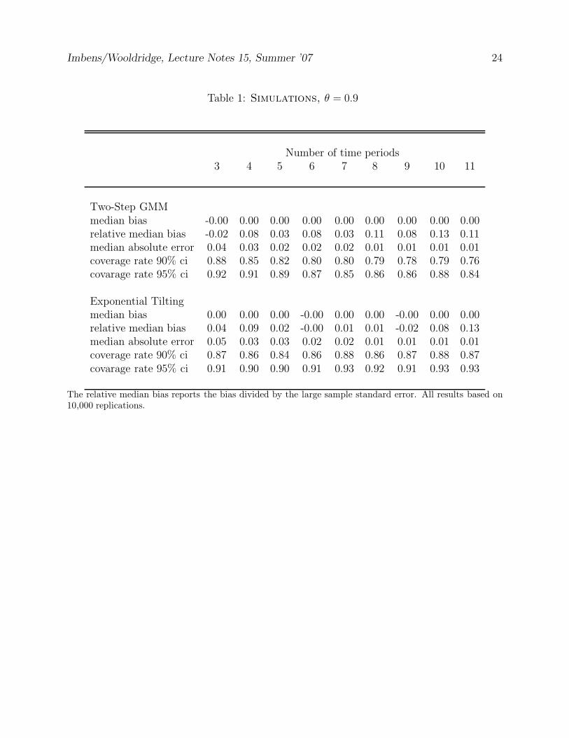
Imbens/Wooldridge, Lecture Notes 15, Summer ’07 24
Table 1: Simulations, θ = 0.9
Number of time periods3 4 5 6 7 8 9 10 11
Two-Step GMMmedian bias -0.00 0.00 0.00 0.00 0.00 0.00 0.00 0.00 0.00relative median bias -0.02 0.08 0.03 0.08 0.03 0.11 0.08 0.13 0.11median absolute error 0.04 0.03 0.02 0.02 0.02 0.01 0.01 0.01 0.01coverage rate 90% ci 0.88 0.85 0.82 0.80 0.80 0.79 0.78 0.79 0.76covarage rate 95% ci 0.92 0.91 0.89 0.87 0.85 0.86 0.86 0.88 0.84
Exponential Tiltingmedian bias 0.00 0.00 0.00 -0.00 0.00 0.00 -0.00 0.00 0.00relative median bias 0.04 0.09 0.02 -0.00 0.01 0.01 -0.02 0.08 0.13median absolute error 0.05 0.03 0.03 0.02 0.02 0.01 0.01 0.01 0.01coverage rate 90% ci 0.87 0.86 0.84 0.86 0.88 0.86 0.87 0.88 0.87covarage rate 95% ci 0.91 0.90 0.90 0.91 0.93 0.92 0.91 0.93 0.93
The relative median bias reports the bias divided by the large sample standard error. All results based on
10,000 replications.