Image Pre-ProcessingImage Pre-Processing

Continuation…Continuation…

Spectral EnhancementSpectral Enhancement

Image Pre-ProcessingImage Pre-Processing

Continuation…Continuation…

Spectral EnhancementSpectral Enhancement

Image Pre-ProcessingImage Pre-ProcessingImage Pre-ProcessingImage Pre-Processing

• Radiometric Enhancement:Radiometric Enhancement:• Image RestorationImage Restoration• Atmospheric CorrectionAtmospheric Correction• Contrast EnhancementContrast Enhancement• Solar Angle AdjustmentSolar Angle Adjustment• Conv. to Exo-Atmos. ReflectanceConv. to Exo-Atmos. Reflectance

• Spectral Enhancement:Spectral Enhancement:• Spectral IndicesSpectral Indices• PCA, IHS, Color Transforms PCA, IHS, Color Transforms • T-Cap, BGWT-Cap, BGW

• Radiometric Enhancement:Radiometric Enhancement:• Image RestorationImage Restoration• Atmospheric CorrectionAtmospheric Correction• Contrast EnhancementContrast Enhancement• Solar Angle AdjustmentSolar Angle Adjustment• Conv. to Exo-Atmos. ReflectanceConv. to Exo-Atmos. Reflectance

• Spectral Enhancement:Spectral Enhancement:• Spectral IndicesSpectral Indices• PCA, IHS, Color Transforms PCA, IHS, Color Transforms • T-Cap, BGWT-Cap, BGW

Consists of processes aimed at the geometric and radiometric Consists of processes aimed at the geometric and radiometric correction, enhancement or standardization of imagery to correction, enhancement or standardization of imagery to improve our ability to interpret qualitatively and improve our ability to interpret qualitatively and quantitatively image components.quantitatively image components.

Consists of processes aimed at the geometric and radiometric Consists of processes aimed at the geometric and radiometric correction, enhancement or standardization of imagery to correction, enhancement or standardization of imagery to improve our ability to interpret qualitatively and improve our ability to interpret qualitatively and quantitatively image components.quantitatively image components.

ImagePre-Processing

• Spatial Enhancement:Spatial Enhancement:• Focal AnalysisFocal Analysis• Edge-DetectionEdge-Detection• High/Low Pass FiltersHigh/Low Pass Filters• Resolution MergesResolution Merges• Statistical FilteringStatistical Filtering• Adaptive FilteringAdaptive Filtering• Texture FiltersTexture Filters

• Geometric CorrectionGeometric Correction• Polynomial TransformationPolynomial Transformation• Ground Control PointsGround Control Points• ReprojectionsReprojections

• Spatial Enhancement:Spatial Enhancement:• Focal AnalysisFocal Analysis• Edge-DetectionEdge-Detection• High/Low Pass FiltersHigh/Low Pass Filters• Resolution MergesResolution Merges• Statistical FilteringStatistical Filtering• Adaptive FilteringAdaptive Filtering• Texture FiltersTexture Filters

• Geometric CorrectionGeometric Correction• Polynomial TransformationPolynomial Transformation• Ground Control PointsGround Control Points• ReprojectionsReprojections

Principal Component AnalysisPrincipal Component AnalysisPCAPCA

Principal Component AnalysisPrincipal Component AnalysisPCAPCA

Principal Components Analysis is a procedure for transforming a set of correlated variables into a new set of uncorrelated variables. This transformation is a rotation of the original axes to new orientations that are orthogonal to each other with little or no correlation between variables

Principal Components Analysis is a procedure for transforming a set of correlated variables into a new set of uncorrelated variables. This transformation is a rotation of the original axes to new orientations that are orthogonal to each other with little or no correlation between variables

Where digital image processing is concerned, this procedure is predominantly exploratory in nature and is used to help in the extraction of features and to reduce dimensionality of data

Where digital image processing is concerned, this procedure is predominantly exploratory in nature and is used to help in the extraction of features and to reduce dimensionality of data

Source: http://umbc7.umbc.edu/~tbenja1/exer1.htmlAfter Lillesand and Keifer, 1994

This scatterplot between two spectral bands implies a strong correlation. One band can be used to predict (to a certain level) the response of the other.

Principal Component Analysis PCA

• Reduces these data into two orthogonal components. The first (CI) contains the common information between bands 1 and 2. The second (CII) contains residual, or independent, information.

• Depending on the amount of covariance between bands 1 and 2, the second component may not contain a significant amount of information and can be eliminated.

This scatterplot between two spectral bands implies a strong correlation. One band can be used to predict (to a certain level) the response of the other.

Principal Component Analysis PCA

• Reduces these data into two orthogonal components. The first (CI) contains the common information between bands 1 and 2. The second (CII) contains residual, or independent, information.

• Depending on the amount of covariance between bands 1 and 2, the second component may not contain a significant amount of information and can be eliminated.

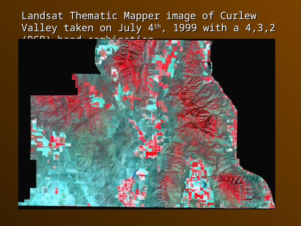
Landsat Thematic Mapper image of Curlew Valley taken on July 4th, 1999 with a 4,3,2 (RGB) band combination.Landsat Thematic Mapper image of Curlew Valley taken on July 4th, 1999 with a 4,3,2 (RGB) band combination.

0.1940 0.0413 -0.3322 0.1961 -0.0783 0.6407 -0.62860.2220 0.1029 -0.4064 0.2209 -0.1421 0.3703 0.75420.3488 0.0925 -0.4950 0.3130 -0.2092 -0.6702 -0.1841

-0.2322 0.9625 0.0450 0.0718 0.1057 -0.0113 -0.03440.5563 0.2023 0.4391 -0.2891 -0.6088 0.0508 -0.00970.2012 -0.0539 0.5330 0.8015 0.1709 0.0179 0.02400.6226 0.0942 -0.0221 -0.2892 0.7204 -0.0117 0.0182

EigenmatrixEigenmatrix

1255.773 72.28%383.448 22.07%45.480 2.62%31.880 1.84%15.707 0.90%3.875 0.22%1.144 0.07%

100.00%

EigenvaluesEigenvalues

The Eigenvalues show the amount of information contained within each component.

The Eigenvalues show the amount of information contained within each component.

The Eigenmatrix contains the coefficients used to calculate each component for the input image. This matrix is a direct result of the covariance between each band.

The Eigenmatrix contains the coefficients used to calculate each component for the input image. This matrix is a direct result of the covariance between each band.

6

1

100_%

pp

p

eigenvalue

xeigenvalueVariance

Factor loadings = what type of component (i.e. visible, infrared) is it?

Rkp: Factor loading

akp:Eigenvector for band k and component p

λp: Eigenvalue for the pth component

Sk: Standard deviation for band k

k

pkp

kp S

xaR

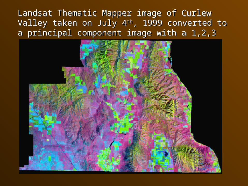
Landsat Thematic Mapper image of Curlew Valley taken on July 4th, 1999 converted to a principal component image with a 1,2,3 (RGB) PCA channel combination.

Landsat Thematic Mapper image of Curlew Valley taken on July 4th, 1999 converted to a principal component image with a 1,2,3 (RGB) PCA channel combination.

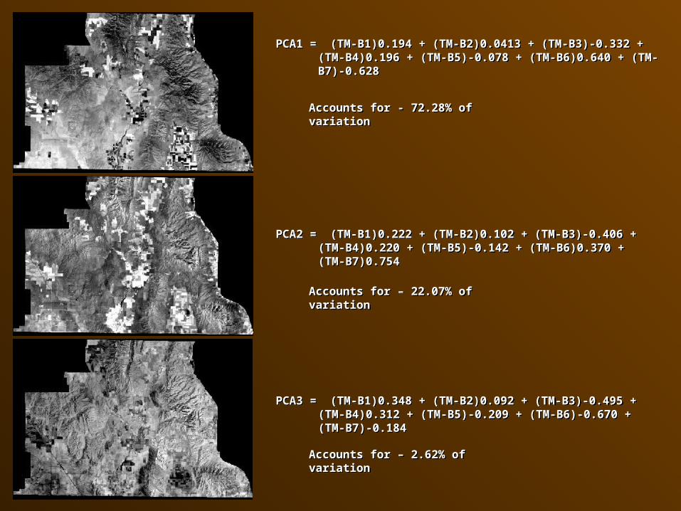
PCA1 = (TM-B1)0.194 + (TM-B2)0.0413 + (TM-B3)‑0.332 + (TM-B4)0.196 + (TM-B5)‑0.078 + (TM-B6)0.640 + (TM-B7)‑0.628

PCA1 = (TM-B1)0.194 + (TM-B2)0.0413 + (TM-B3)‑0.332 + (TM-B4)0.196 + (TM-B5)‑0.078 + (TM-B6)0.640 + (TM-B7)‑0.628

PCA2 = (TM-B1)0.222 + (TM-B2)0.102 + (TM-B3)‑0.406 + (TM-B4)0.220 + (TM-B5)‑0.142 + (TM-B6)0.370 + (TM-B7)0.754

PCA2 = (TM-B1)0.222 + (TM-B2)0.102 + (TM-B3)‑0.406 + (TM-B4)0.220 + (TM-B5)‑0.142 + (TM-B6)0.370 + (TM-B7)0.754

PCA3 = (TM-B1)0.348 + (TM-B2)0.092 + (TM-B3)‑0.495 + (TM-B4)0.312 + (TM-B5)‑0.209 + (TM-B6)-0.670 + (TM-B7)-0.184

PCA3 = (TM-B1)0.348 + (TM-B2)0.092 + (TM-B3)‑0.495 + (TM-B4)0.312 + (TM-B5)‑0.209 + (TM-B6)-0.670 + (TM-B7)-0.184

Accounts for - 72.28% of variationAccounts for - 72.28% of variation

Accounts for – 22.07% of variationAccounts for – 22.07% of variation

Accounts for – 2.62% of variationAccounts for – 2.62% of variation

PCA4 = (TM-B1)-0.232 + (TM-B2)0.962 + (TM-B3)0.045 + (TM-B4)0.071 + (TM-B5)0.105 + (TM-B6)-0.011 + (TM-B7)-0.034

PCA4 = (TM-B1)-0.232 + (TM-B2)0.962 + (TM-B3)0.045 + (TM-B4)0.071 + (TM-B5)0.105 + (TM-B6)-0.011 + (TM-B7)-0.034

PCA5 = (TM-B1)0.556 + (TM-B2)0.202 + (TM-B3)0.439 + (TM-B4)-0.289 + (TM-B5)-0.608 + (TM-B6)0.050 + (TM-B7)-0.009

PCA5 = (TM-B1)0.556 + (TM-B2)0.202 + (TM-B3)0.439 + (TM-B4)-0.289 + (TM-B5)-0.608 + (TM-B6)0.050 + (TM-B7)-0.009

PCA5 = (TM-B1)0.201 + (TM-B2)-0.053 + (TM-B3)0.533 + (TM-B4)0.801 + (TM-B5)0.170 + (TM-B6)0.017 + (TM-B7)0.023

PCA5 = (TM-B1)0.201 + (TM-B2)-0.053 + (TM-B3)0.533 + (TM-B4)0.801 + (TM-B5)0.170 + (TM-B6)0.017 + (TM-B7)0.023

Accounts for – 1.84% of variationAccounts for – 1.84% of variation

Accounts for – 0.90% of variationAccounts for – 0.90% of variation

Accounts for – 0.22% of variationAccounts for – 0.22% of variation

PCA5 = (TM-B1)0.622 + (TM-B2)-0.094 + (TM-B3)-0.022 + (TM-B4)-0.289 + (TM-B5)0.720 + (TM-B6)-0.011 + (TM-B7)0.018

PCA5 = (TM-B1)0.622 + (TM-B2)-0.094 + (TM-B3)-0.022 + (TM-B4)-0.289 + (TM-B5)0.720 + (TM-B6)-0.011 + (TM-B7)0.018

Accounts for – 0.07% of variationAccounts for – 0.07% of variation

Components 1 – 3 account for 96.97% of the total variationComponents 1 – 3 account for 96.97% of the total variation

While the remaining components only account for a combined 3.03% of the total variation, there may be spatial information available.

While the remaining components only account for a combined 3.03% of the total variation, there may be spatial information available.