chapter 16: spectral enhancement of landsat imagery remote...

Chapter 16: Spectral Enhancement of Landsat Imagery

Remote Sensing Analysis

in an

ArcMap Environment

Tammy E. Parece

Remote Sensing in an ArcMap Environment

Tammy Parece James Campbell

John McGee

This workbook is available online as text (.pdf’s) and short video tutorials via: http://www.virginiaview.net/education.html

Image source: landsat.usgs.gov

NSF DUE 0903270; 1205110

http://www.virginiaview.net/education.html

The project described in this publication was supported by Grant Number G14AP00002 from the Department of the Interior, United States Geological Survey to AmericaView. Its contents are solely the responsibility of the authors; the views and conclusions contained in this document are those of the authors and should not be interpreted as representing the opinions or policies of the U.S. Government. Mention of trade names or commercial products does not constitute their endorsement by the U.S. Government.

Remote Sensing in an ArcMap Environment 16. Spectral Enhancement of Landsat Imagery

The instructional materials contained within these documents are copyrighted property of VirginiaView, its partners and other participating AmericaView consortium members. These

materials may be reproduced and used by educators for instructional purposes. No permission is granted to use the materials for paid consulting or instruction where a fee is collected.

Reproduction or translation of any part of this document beyond that permitted in Section 107 or 108 of the 1976 United States Copyright Act without the permission of the copyright

owner(s) is unlawful.

Introduction

Spectral signatures refer to the range of reflected radiation wavelengths for different objects collected by the various Landsat bands. For example - spectral signatures can be used to distinguish between man-made objects and different types of vegetation. (For more information on different objects’ spectral signatures – see Campbell and Wynne, 2011 or Keranen and Kolvoord, 2013). Spectral enhancement is the process of creating new spectral data from available bands. New data are created on a pixel-by-pixel basis by applying an operation (e.g., subtraction, division) to corresponding pixels in existing bands. Spectral enhancement only applies to multi-band images. This technique is typically used to:

• Extract new bands of data that are more interpretable to the eye (in some cases to classifiers as well)

• Reduce redundancy in a multi-spectral dataset by compressing bands of data that are similar (principal component analysis)

• Display a wider variety of information in the three available colors of the visible spectrum (R,G,B)

The most widely used techniques of spectral enhancement are:

• Spectral Ratios and Indices - Performs band ratios that are commonly used in vegetation and mineral studies;

• Principal Components Analysis (PCA) - Compresses redundant data values into fewer bands which are often more interpretable than the source data (we will not perform a PCA in this tutorial);

• Tasseled Cap – Transforms and rotates the data structure axes to optimize data viewing for vegetation studies.

We will explore band ratios, vegetation indices, and tasseled cap. Remember the differences between the three types of enhancement techniques:

• Radiometric Enhancement - Enhancing images based on the values of individual pixels

179 | P a g e


• Spatial Enhancement - Enhancing images based on the values of individual and neighboring pixels.

• Spectral Enhancement - Enhancing images by transforming the values of each pixel on a multi-band basis (for multi-band images).

Band Ratios Avery, Thomas Eugene and Graydon Lennis Berlin, Fundamentals of Remote Sensing and Aerial Interpretation. 5th ed. New Jersey: Prentice-Hall Inc, 1992. 4 / 3 Ratio - (NIR/Red) - enhances the presence of vegetation. The brighter the tones the

denser the vegetation. 5 / 2 Ratio - (MIR/Green) – To detect moisture levels. 2 / 5 Ration – (Green/MIR) – To pull out water bodies. 3 / 7 Ratio - (Red/MIR) – To see differences in water turbidity. 3 / 1 Ratio – (Red/Blue) – To detect ferric iron rocks. 5 / 7 Ratio – (MIR / MIR) – To detect clay rich rocks. Aside from the 5 ratios listed here there are 25 other possible ratios to perform with Landsat TM imagery. The important thing to remember with ratios is the scanner system that produced the imagery. Landsat TM ratios will use different band numbers from those of Landsat MSS, SPOT, or IRS (India Remote Sensing).

180 | P a g e


Creating Band Ratios

Open a new map document and add the seven separate images that you received when

you unzipped the downloaded Landsat scene. To create a band ratio, you will be using the

Spatial Analyst Toolset, so be sure that the extension and toolbars are

turned on, your Toolbox is open, and your workspaces are set. It does

not matter what order the bands are listed in your Table of Contents. For

simple indices, you will be using Spatial Analyst/Math/Trigonometric

tools. Within these tools is divide, plus, square, square root, etc.

PLEASE NOTE – ArcGIS treats the pixel values for Landsat

Imagery as integers. As such, when performing math operations, the

results are integers, usually rounded down. We do not want our results

to be integers but real numbers (numbers with decimal points). This

means we need to change our images to floating point images. You do

not need to accomplish this on all bands for this tutorial, only the bands

you are going to use to create ratios.

Left-click on Float (yellow circle)

You get the following window:

181 | P a g e


Left-click on the down arrow at the end of the Input Raster line, choose the band that

you wish to convert. In this case, we chose band 4 (B4). For the Output raster, it should fill

with your workspace and after your workspace, name your file. In this case, we have named it

Float_B4. The name cannot begin with a number and it cannot have any spaces or special

characters. Left-click OK.

Once you click OK, wait for ArcGIS to process it and it will automatically add your new

file to your Table of Contents and map document window.

In the Table of Contents, this new file still looks like an

integer, but if you use the

Identify button and click

anywhere on the image, you

see that decimal points have

now been added to the pixel value.

182 | P a g e


Now, let’s do your first ratio – 4 / 3. Make sure you have make floating point images for

both bands before you proceed to the next step.

Once you have your two new images, you want to use Spatial

Analyst/Math/Trigonometric/Divide. Double-left-click on that tool and the following dialog

box opens. Enter the images as shown. Remember to name your new file appropriately.

Click OK. ArcMap will automatically add the new image to your Table of Contents and

map document window when the processing is complete. Again,

it looks like we have integers but if you use Identify and click on

any pixel, you will find a decimal

number.

183 | P a g e


Let’s look at the image. Remember from above, 4 / 3 Ratio - (NIR/Red) - enhances the

presence of vegetation; the brighter the tones, the denser the vegetation. Do you remember

from prior Tutorials, what was present in the mountain areas? Our scene is from March, so leaf-

off, except for conifers.

Let’s do one more together - 3 / 7 Ratio - (Red/MIR) – To see differences in water

turbidity. (Don’t forget, we need a floating point image for each band).

Using Spatial Analyst/Math/Trigonometric/Divide, your dialog box should looks as

follows:

184 | P a g e


Click OK.

Areas of water are bright. Let’s zoom into Smith Mountain Lake.

185 | P a g e


What do

you see? Why

would areas

leading into the

lake be brighter?

What about at the

dam area?

Which

areas are more

turbid?

You can do any of the simple ratios using this tool set. (Simple ratios are those that

require one function only.) You can do more complex ones using these tools, but you do it step

by step and create images one at a time and then use that image in the next step. Raster

calculator allows you to do a complex calculation in one step. We will see one of these indices

in the next section.

Vegetation Indices

Another spectral enhancement is a vegetation index. Although within ArcGIS, you can

create many different many indices, we will only look at three of them: IR/R, square root (IR/R),

& NDVI.

186 | P a g e


We have actually already calculated when we did the 4 / 3 ratio above. Which band is

IR? Which band is R? (4 is IR and 3 is R). So when we calculated the ratio 4 / 3 above, we

calculated this ratio. Remember - 4 / 3 Ratio - (NIR/Red) defines the presence of vegetation;

the brighter the tones, the denser the vegetation.

Let’s look at the square root of IR/R next. We can do this

two different ways, because we have already calculated the IR/R.

The first way would be to take the square root of this result.

Double-left-click on this tool, your dialog box should look

as follows and click OK.

187 | P a g e


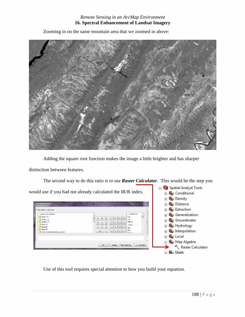
Zooming in on the same mountain area that we zoomed in above:

Adding the square root function makes the image a little brighter and has sharper

distinction between features.

The second way to do this ratio is to use Raster Calculator. This would be the step you

would use if you had not already calculated the IR/R index.

Use of this tool requires special attention to how you build your equation.

188 | P a g e


Your dialog box should appear as follows. Watch carefully where the parentheses are

placed! With proper placement of parentheses, you can create much more complex equations.

There is absolutely no difference between the two methods, except for the number of steps. Layers in the Table of Contents Value of a select pixel

I did make an error when I used Raster Calculator.

Can you see what I did? I failed to rename my file

before I clicked okay, so Raster Calculator created its own name for the new file. You must be

careful to appropriately name your image, so you can identify it later.

189 | P a g e


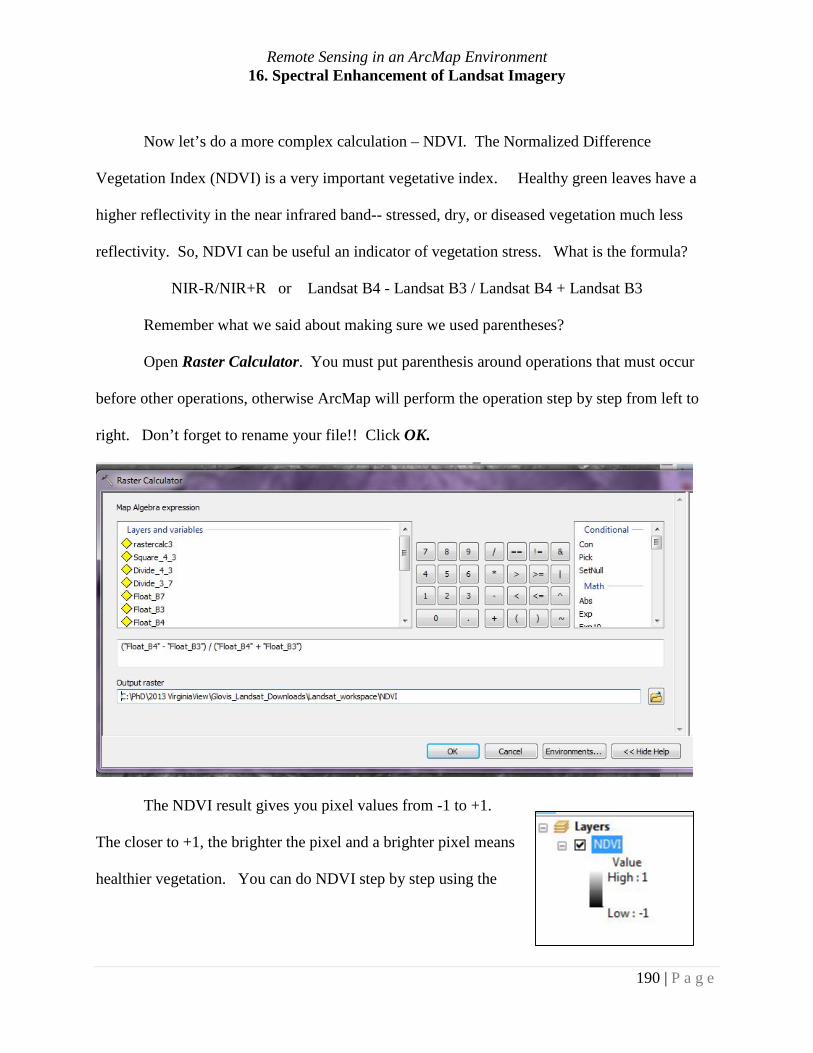
Now let’s do a more complex calculation – NDVI. The Normalized Difference

Vegetation Index (NDVI) is a very important vegetative index. Healthy green leaves have a

higher reflectivity in the near infrared band-- stressed, dry, or diseased vegetation much less

reflectivity. So, NDVI can be useful an indicator of vegetation stress. What is the formula?

NIR-R/NIR+R or Landsat B4 - Landsat B3 / Landsat B4 + Landsat B3

Remember what we said about making sure we used parentheses?

Open Raster Calculator. You must put parenthesis around operations that must occur

before other operations, otherwise ArcMap will perform the operation step by step from left to

right. Don’t forget to rename your file!! Click OK.

The NDVI result gives you pixel values from -1 to +1.

The closer to +1, the brighter the pixel and a brighter pixel means

healthier vegetation. You can do NDVI step by step using the

190 | P a g e


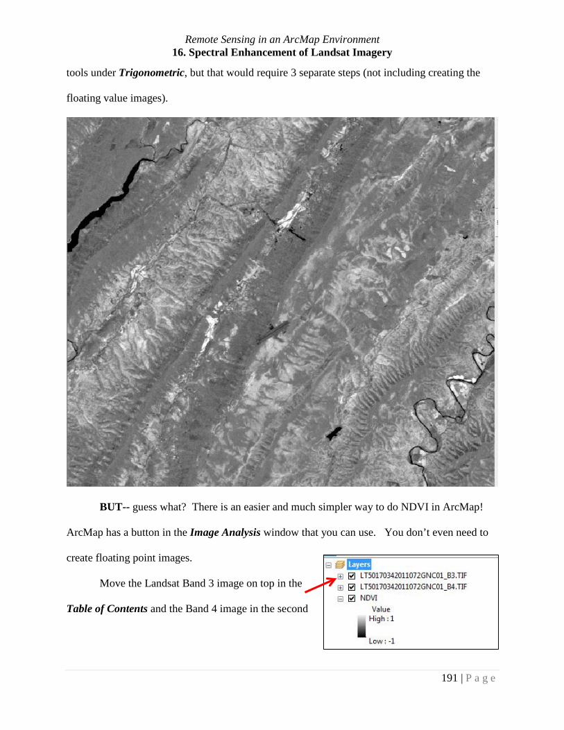
tools under Trigonometric, but that would require 3 separate steps (not including creating the

floating value images).

BUT-- guess what? There is an easier and much simpler way to do NDVI in ArcMap!

ArcMap has a button in the Image Analysis window that you can use. You don’t even need to

create floating point images.

Move the Landsat Band 3 image on top in the

Table of Contents and the Band 4 image in the second

191 | P a g e


to top spot. Open your Image Analysis window. The images must be in the correct order to get

the correct results!

This also puts the images on top in the Image

Analysis window. Highlight the two images.

Band 3 must be the first one! Now, look under

Processing, a button with a Leaf is now enabled!

This is the NDVI button (yellow circle). Before

you click, we need to check one thing. Go to

Options (red circle). Look an NDVI Tab! Make

sure that Use Wavelength is unchecked and

Scientific Output is checked. Then click OK.

Then left-click on the Leaf button.

192 | P a g e


We got the exact same results from this

method as with Raster Calculator, but that

result is difficult to see just by looking at the

Table of Contents.

Let’s look at individual pixels values using Identify.

First, we look at a water pixel:

We have a negative value: - 0.375 for

both. Why a negative for water?

Remember, this is a vegetation index and

a low value for water is normal. What

could be an exception? (Answer – an

extreme algae bloom or a prolific invasive water plant)

Let’s look at an extremely bright pixel:

We have a positive value: 0.532468 for both.

You have now learned two ways to calculate NDVI. Both methods give you the same

numeric and image results. But there is one major difference between the two resultant images.

Raster calculator file

Image Analysis file

193 | P a g e


Do you remember what they are? Hint – one was created from Raster Calculator and one from

using the Image Analysis Processing button. So, which image is permanent and which is only

temporary?

Tasseled Cap Transformation The Tasseled Cap Transformation is a spectral enhancement aimed primarily at analyzing agricultural vegetation. The principle behind the Tasseled Cap calculation is the notion that the bands in a multispectral image are interrelated and can be viewed as planes in multidimensional space with pixel values placed in the respective planes. The clustering of values resulting from such scattering creates data structures shaped in a multidimensional hyperellipsoid, which is defined by the principal axes. By selecting pairs of principal axes and using them as the viewer’s x and y axes, data structures representing different vegetation information content can be seen. Out of the 6 data structures created by the Tasseled Cap analysis, brightness, greenness and wetness are or the importance for this exercise. The output values for the data structures are calculated through a linear equation with the coefficients specific to the sensor that produced the image. Tasseled Cap index is calculated from data of the six TM bands; however, three of the six bands are often used: band 1 (brightness, measure of soil) band 2 (greenness, measure of vegetation) band 3 (wetness, interrelationship of soil and canopy moisture)

Within ArcGIS 10.X the Tasseled Cap Transformation is accomplished using Functions. Functions are more complex operations within ArcGIS and beyond the scope of this tutorial. You can refer to ArcGIS Help for more information. Now that you have learned about the different types of enhancement and how to

accomplish these in ArcGIS, you are ready to proceed with the tutorials on Change Detection

and Image Classification.

194 | P a g e

chapter 16: spectral enhancement of landsat imagery remote...

Documents