9/13/10  

1  

Image Enhancement in the Spatial Domain

Jesus J. Caban

Outline 1.  Need to know the papers you are presenting by 9/15/10

2.  Questions about homework?

3.  Today’s Topic: Image Enhancement

9/13/10  

2  

Introduction: Image Enhancement   Goals:

 Noise Removal   Feature Enhancement  Visualization

  Common Techniques   Simple (conceptually and computationally)  Generally applicable (domain independent)  Often heuristic (difficult to define final image “quality”)

  The spatial domain:   The image plane   For a digital image is a Cartesian coordinate system of discrete rows and columns.

At the intersection of each row and column is a pixel. Each pixel has a value, which we will call intensity.

  The frequency domain :   A (2-dimensional) discrete Fourier transform of the spatial domain

  Enhancement :   To “improve” the usefulness of an image by using some transformation on the

image.   Often the improvement is to help make the image “better” looking, such as

increasing the intensity or contrast.

Image Enhancement: Spatial Domain

9/13/10  

3  

  A mathematical representation of spatial domain enhancement:

where f(x, y): the input image g(x, y): the processed image T: an operator on f, defined over some neighborhood of (x, y)

Image Enhancement

The Image Histogram   The image histogram shows the frequency distribution of

gray values in the image.

  Histogram discards spatial information and shows relative frequency of occurrence of gray values

0 1 2 3 4 5 6 7

Gray Value

2 2 4 6 7 8 6 1

Count 0.05 0.05 .11 .17 .20 .22 .17 .03

Rel. Freq.

0 3 3 2 5 5 1 1 0 3 4 5 2 2 2 4 4 4 3 3 4 4 5 5 3 4 5 5 6 6 7 6 6 6 6 5

9/13/10  

4  

Image Histogram

0

1

2

3

4

5

6

7

8

9

0 1 2 3 4 5 6 7

0 3 3 2 5 5 1 1 0 3 4 5 2 2 2 4 4 4 3 3 4 4 5 5 3 4 5 5 6 6 7 6 6 6 6 5

0 0.1 0.2 0.3 0.4 0.5 0.6 0.7 0.8 0.9

1

0 1 2 3 4 5 6 7

€

H(i) = M *Ni=Imin

Imax

∑

Image size: M * N

Histogram Processing

Let’s start with point processing

9/13/10  

5  

Enhancement through Point Processing

  Based on the intensity of a single pixel only as opposed to a neighborhood or region

  Straightforward methods typically used to globally adjust  Contrast

  The difference in gray levels or luminance value over some area of the image

  Contrast Range: Imax – Imin

  Contrast Ratio: Imax/Imin

 Color   Intensity

Contrast Enhancement: Scaling   General Idea:

 Apply a linear (non-linear) scaling transform to every point in the image to obtain a new (modified) image.

9/13/10  

6  

Gray-level Transformation

0 255

255

0

Input Gray Level

Out

put G

ray

Leve

l

Gray-level Transformation

9/13/10  

7  

  Let the range of gray level be [0, L-1], then

Image Negatives

9/13/10  

8  

Gray-level : Manipulation

1) Contrast Stretching 2) Gray-level Slicing

1) Contrast Stretching

9/13/10  

9  

2) Gray-level Slicing

Contrast Stretching: How?

9/13/10  

10  

  Histogram equalization:   To improve the contrast of an image   To transform an image in such a way that the transformed image has a nearly

uniform distribution of pixel values

Histogram Equalization

Equalization Transformation Function

9/13/10  

11  

Histogram Equalization 1) Probability of Occurrence

2) Create Cumulative Distribution Function

3) Map old value to new value

Equalization Examples

9/13/10  

12  

Histogram Equalization

Histogram Equalization - Limitations

9/13/10  

13  

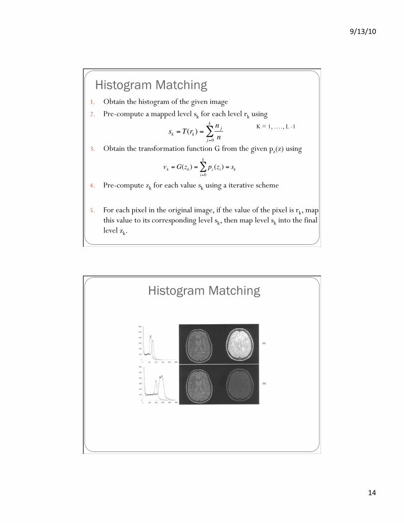
  Histogram matching is similar to histogram equalization, except that instead of trying to make the output image have a flat histogram, we would like it to have a histogram of a specified shape, say pz(z).

1) Histogram Matching

Histogram Matching

9/13/10  

14  

Histogram Matching 1.  Obtain the histogram of the given image 2.  Pre-compute a mapped level sk for each level rk using

K = 1, …., L -1

3.  Obtain the transformation function G from the given pz(z) using

4.  Pre-compute zk for each value sk using a iterative scheme

5.  For each pixel in the original image, if the value of the pixel is rk, map this value to its corresponding level sk, then map level sk into the final level zk.

€

sk = T(rk ) =n j

nj=0

k

∑

€

vk =G(zk ) = pz (zi) = ski=0

k

∑

Histogram Matching

9/13/10  

15  

Histogram Matching

  The histogram processing methods discussed previously are global, in the sense that pixels are modified by a transformation function based on the gray-level content of an entire image.

  However, there are cases in which it is necessary to enhance details over small areas in an image.

original

2) Local Enhancement

global Local (7x7)

9/13/10  

16  

Operations

Image Operations

  Just as with numbers, we can apply different operations to an image  Addition: +   Subtraction: -  Multiplication: *  And: &&  Or: ||  Derivative:

 Average  Mean

€

dxdy

9/13/10  

17  

Enhancement Using Logic Operations

AND

OR

Image Subtraction

9/13/10  

18  

 When taking pictures in reduced lighting (i.e., low illumination), image noise becomes apparent.

  A noisy image g(x,y) can be defined by

where f (x, y): an original image : the addition of noise

 One simple way to reduce this granular noise is to take several identical pictures and average them, thus smoothing out the randomness.

Image Averaging

AVG =

3

Image Averaging

9/13/10  

19  

  In general, linear filtering of an image f of size MxN is given by

  This concept called convolution. Filter masks are sometimes called convolution masks or convolution kernels.

Basics of Spatial Filtering

The Spatial Filtering Process

r s t

u v w

x y z

Origin x

y Image f (x, y)

eprocessed = v*e + r*a + s*b + t*c + u*d + w*f + x*g + y*h + z*i

Filter Simple 3*3

Neighbourhood e 3*3 Filter

a b c

d e f

g h i Original Image

Pixels

*

The above is repeated for every pixel in the original image to generate the filtered image

9/13/10  

20  

Smoothing Spatial Filters  One of the simplest spatial filtering operations we can perform is a smoothing operation

  Simply average all of the pixels in a neighbourhood around a central value

  Especially useful in removing noise from images

 Also useful for highlighting gross detail

1/9 1/9 1/9

1/9 1/9

1/9

1/9 1/9

1/9

Simple averaging filter

Smoothing Spatial Filtering 1/9

1/9 1/9

1/9 1/9  

1/9

1/9 1/9

1/9

Origin x

y Image f (x, y)

e = 1/9*106 + 1/9*104 + 1/9*100 + 1/9*108 + 1/9*99 + 1/9*98 + 1/9*95 + 1/9*90 + 1/9*85

= 98.3333

Filter Simple 3*3

Neighbourhood 106

104

99

95

100 108

98

90 85

1/9 1/9

1/9

1/9 1/9

1/9

1/9 1/9

1/9

3*3 Smoothing Filter

104 100 108

99 106 98

95 90 85

Original Image Pixels

*

The above is repeated for every pixel in the original image to generate the smoothed image

9/13/10  

21  

Moving Window Transform: Example

original 3x3 average

Moving Window Transform: Example

original 3x3 average

9/13/10  

22  

Image Smoothing Example

 The image at the top left is an original image of size 500*500 pixels  The subsequent images show the image after filtering with an averaging filter of increasing sizes

  3, 5, 9, 15 and 35

 Notice how detail begins to disappear

Image Smoothing Example

9/13/10  

23  

  In general, linear filtering of an image f of size MxN is given by

  This concept called convolution. Filter masks are sometimes called convolution masks or convolution kernels.

Basics of Spatial Filtering

1/9 1/9 1/9

1/9 1/9

1/9

1/9 1/9

1/9

Another Smoothing Example  By smoothing the original image we get rid of lots of the finer detail which leaves only the gross features for thresholding

Original Image Smoothed Image Thresholded Image

9/13/10  

24  

Weighted Smoothing Filters  More effective smoothing filters can be generated by allowing different pixels in the neighbourhood different weights in the averaging function

  Pixels closer to the central pixel are more important

 Often referred to as a weighted averaging

1/16 2/16 1/16

2/16 4/16

2/16

1/16 2/16

1/16

Weighted averaging filter

  Order-statistic filters  Median filter: to reduce impulse noise (salt-and-pepper noise)

Order Statistic Filters

1/9 1/9 1/9

1/9 1/9

1/9

1/9 1/9

1/9

9/13/10  

25  

Gaussian Smoothing

Derivatives Differentiation measures the rate of change of a function Let’s consider a simple 1 dimensional example

9/13/10  

26  

Spatial Differentiation

A B

1st Order Derivative The formula for the 1st derivative of a function is as follows:

It’s just the difference between subsequent values and measures the rate of change of the function

9/13/10  

27  

1st Order Derivative

5 5 4 3 2 1 0 0 0 6 0 0 0 0 1 3 1 0 0 0 0 7 7 7 7

0 -1 -1 -1 -1 0 0 6 -6 0 0 0 1 2 -2 -1 0 0 0 7 0 0 0

2nd Order Derivative

The formula for the 2nd derivative of a function is as follows:

Simply takes into account the values both before and after the current value

9/13/10  

28  

2nd Order Derivative

5 5 4 3 2 1 0 0 0 6 0 0 0 0 1 3 1 0 0 0 0 7 7 7 7

-1 0 0 0 0 1 0 6 -12 6 0 0 1 1 -4 1 1 0 0 7 -7 0 0

Using Second Derivatives For Image Enhancement The 2nd derivative is more useful for image enhancement than the 1st derivative

  Stronger response to fine detail   Simpler implementation

9/13/10  

29  

The Laplacian The Laplacian is defined as follows:

where the partial 1st order derivative in the x direction is defined as follows:

and in the y direction as follows:

The Laplacian So, the Laplacian can be given as follows:

We can easily build a filter based on this

0 1 0

1 -4 1

0 1 0

9/13/10  

30  

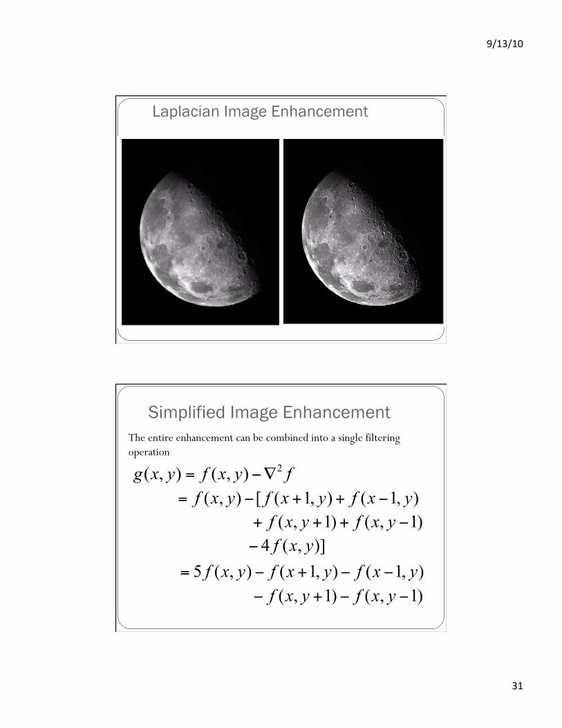
The Laplacian Applying the Laplacian to an image we get a new image that highlights edges and other discontinuities

Original Image

Laplacian Filtered Image

Laplacian Filtered Image

Scaled for Display

Laplacian Image Enhancement

In the final sharpened image edges and fine detail are much more obvious

- =

Original Image

Laplacian Filtered Image

Sharpened Image

9/13/10  

31  

Laplacian Image Enhancement

Simplified Image Enhancement The entire enhancement can be combined into a single filtering operation

9/13/10  

32  

Simplified Image Enhancement (cont…) This gives us a new filter which does the whole job for us in one step

0 -1 0

-1 5 -1

0 -1 0

Simplified Image Enhancement

9/13/10  

33  

Variants On The Simple Laplacian There are lots of slightly different versions of the Laplacian that can be used:

0 1 0

1 -4 1

0 1 0

1 1 1

1 -8 1

1 1 1

-1 -1 -1

-1 9 -1

-1 -1 -1

Simple Laplacian

Variant of Laplacian

Acknowledgements   Some of the images and diagrams have been taken from the

Gonzalez et al, “Digital Image Processing” book.