image enhancement in the spatial domain - umd...
TRANSCRIPT

75
3 Image Enhancement in the Spatial Domain
It makes all the difference whether one sees darknessthrough the light or brightness through the shadows.
David Lindsay
PreviewThe principal objective of enhancement is to process an image so that the re-sult is more suitable than the original image for a specific application.The wordspecific is important, because it establishes at the outset that the techniques dis-cussed in this chapter are very much problem oriented. Thus, for example, amethod that is quite useful for enhancing X-ray images may not necessarily bethe best approach for enhancing pictures of Mars transmitted by a space probe.Regardless of the method used, however, image enhancement is one of the mostinteresting and visually appealing areas of image processing.
Image enhancement approaches fall into two broad categories: spatial domainmethods and frequency domain methods.The term spatial domain refers to theimage plane itself, and approaches in this category are based on direct manipu-lation of pixels in an image. Frequency domain processing techniques are basedon modifying the Fourier transform of an image. Spatial methods are covered inthis chapter, and frequency domain enhancement is discussed in Chapter 4. En-hancement techniques based on various combinations of methods from thesetwo categories are not unusual.We note also that many of the fundamental tech-niques introduced in this chapter in the context of enhancement are used insubsequent chapters for a variety of other image processing applications.
There is no general theory of image enhancement. When an image isprocessed for visual interpretation, the viewer is the ultimate judge of how well
GONZ03-075-146.II 29-08-2001 13:42 Page 75
76 Chapter 3 � Image Enhancement in the Spatial Domain
Origin
x
Image f(x, y)
(x, y)
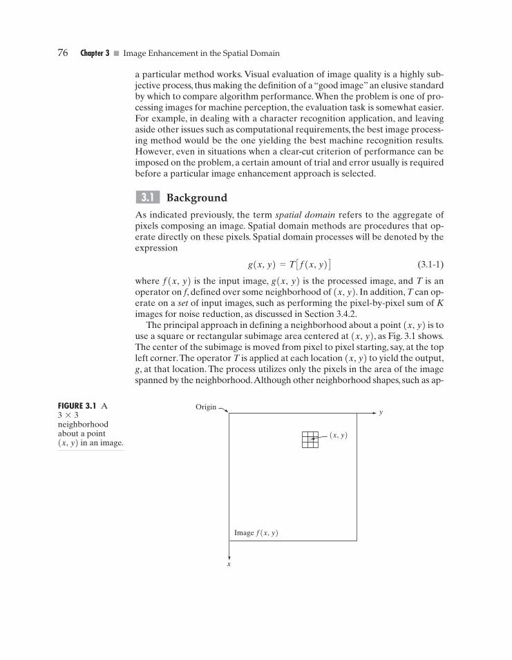
yFIGURE 3.1 A3*3neighborhoodabout a point(x, y) in an image.
a particular method works. Visual evaluation of image quality is a highly sub-jective process, thus making the definition of a “good image” an elusive standardby which to compare algorithm performance.When the problem is one of pro-cessing images for machine perception, the evaluation task is somewhat easier.For example, in dealing with a character recognition application, and leavingaside other issues such as computational requirements, the best image process-ing method would be the one yielding the best machine recognition results.However, even in situations when a clear-cut criterion of performance can beimposed on the problem, a certain amount of trial and error usually is requiredbefore a particular image enhancement approach is selected.
Background
As indicated previously, the term spatial domain refers to the aggregate ofpixels composing an image. Spatial domain methods are procedures that op-erate directly on these pixels. Spatial domain processes will be denoted by theexpression
(3.1-1)
where f(x, y) is the input image, g(x, y) is the processed image, and T is anoperator on f, defined over some neighborhood of (x, y). In addition, T can op-erate on a set of input images, such as performing the pixel-by-pixel sum of Kimages for noise reduction, as discussed in Section 3.4.2.
The principal approach in defining a neighborhood about a point (x, y) is touse a square or rectangular subimage area centered at (x, y), as Fig. 3.1 shows.The center of the subimage is moved from pixel to pixel starting, say, at the topleft corner.The operator T is applied at each location (x, y) to yield the output,g, at that location. The process utilizes only the pixels in the area of the imagespanned by the neighborhood.Although other neighborhood shapes, such as ap-
g(x, y) = T Cf(x, y) D
3.1
GONZ03-075-146.II 29-08-2001 13:42 Page 76

3.1 � Background 77
T(r)T(r)
mr
s=T(r) s=T(r)
Dar
kL
ight
Dar
kL
ight
Dark Lightm
Dark Light
r
FIGURE 3.2 Gray-leveltransformationfunctions forcontrastenhancement.
proximations to a circle, sometimes are used, square and rectangular arrays areby far the most predominant because of their ease of implementation.
The simplest form of T is when the neighborhood is of size 1*1 (that is, asingle pixel). In this case, g depends only on the value of f at (x, y), and T be-comes a gray-level (also called an intensity or mapping) transformation func-tion of the form
(3.1-2)
where, for simplicity in notation, r and s are variables denoting, respectively,the gray level of f(x, y) and g(x, y) at any point (x, y). For example, if T(r) hasthe form shown in Fig. 3.2(a), the effect of this transformation would be to pro-duce an image of higher contrast than the original by darkening the levels belowm and brightening the levels above m in the original image. In this technique,known as contrast stretching, the values of r below m are compressed by thetransformation function into a narrow range of s, toward black.The opposite ef-fect takes place for values of r above m. In the limiting case shown in Fig. 3.2(b),T(r) produces a two-level (binary) image. A mapping of this form is called athresholding function. Some fairly simple, yet powerful, processing approachescan be formulated with gray-level transformations. Because enhancement atany point in an image depends only on the gray level at that point, techniquesin this category often are referred to as point processing.
Larger neighborhoods allow considerably more flexibility. The general ap-proach is to use a function of the values of f in a predefined neighborhood of(x, y) to determine the value of g at (x, y). One of the principal approaches inthis formulation is based on the use of so-called masks (also referred to as filters,kernels, templates, or windows). Basically, a mask is a small (say, 3*3) 2-Darray, such as the one shown in Fig. 3.1, in which the values of the mask coeffi-cients determine the nature of the process, such as image sharpening. En-hancement techniques based on this type of approach often are referred to asmask processing or filtering. These concepts are discussed in Section 3.5.
s = T(r)
a b
GONZ03-075-146.II 29-08-2001 13:42 Page 77

78 Chapter 3 � Image Enhancement in the Spatial Domain
Some Basic Gray Level Transformations
We begin the study of image enhancement techniques by discussing gray-leveltransformation functions.These are among the simplest of all image enhancementtechniques.The values of pixels, before and after processing, will be denoted by rand s, respectively. As indicated in the previous section, these values are relatedby an expression of the form s=T(r), where T is a transformation that maps apixel value r into a pixel value s. Since we are dealing with digital quantities, val-ues of the transformation function typically are stored in a one-dimensional arrayand the mappings from r to s are implemented via table lookups. For an 8-bit en-vironment, a lookup table containing the values of T will have 256 entries.
As an introduction to gray-level transformations, consider Fig. 3.3, whichshows three basic types of functions used frequently for image enhancement: lin-ear (negative and identity transformations), logarithmic (log and inverse-logtransformations), and power-law (nth power and nth root transformations).Theidentity function is the trivial case in which output intensities are identical toinput intensities. It is included in the graph only for completeness.
3.2.1 Image NegativesThe negative of an image with gray levels in the range [0, L-1] is obtained by usingthe negative transformation shown in Fig. 3.3, which is given by the expression
(3.2-1)s = L - 1 - r.
3.2
0
Identity
0L/4
L/4
L/2
L/2
3L/4
3L/4
L-1
L-1
Input gray level, r
Out
put g
ray
leve
l, s Log
Negative
Inverse log
nth power
nth root
FIGURE 3.3 Somebasic gray-leveltransformationfunctions used forimageenhancement.
GONZ03-075-146.II 29-08-2001 13:42 Page 78

3.2 � Some Basic Gray Level Transformations 79
FIGURE 3.4(a) Originaldigitalmammogram.(b) Negativeimage obtainedusing the negativetransformation inEq. (3.2-1).(Courtesy of G.E.Medical Systems.)
Reversing the intensity levels of an image in this manner produces the equiva-lent of a photographic negative. This type of processing is particularly suitedfor enhancing white or gray detail embedded in dark regions of an image, es-pecially when the black areas are dominant in size. An example is shown inFig. 3.4. The original image is a digital mammogram showing a small lesion. Inspite of the fact that the visual content is the same in both images, note howmuch easier it is to analyze the breast tissue in the negative image in this par-ticular case.
3.2.2 Log TransformationsThe general form of the log transformation shown in Fig. 3.3 is
(3.2-2)
where c is a constant, and it is assumed that r � 0. The shape of the log curvein Fig. 3.3 shows that this transformation maps a narrow range of low gray-levelvalues in the input image into a wider range of output levels.The opposite is trueof higher values of input levels. We would use a transformation of this type toexpand the values of dark pixels in an image while compressing the higher-levelvalues. The opposite is true of the inverse log transformation.
Any curve having the general shape of the log functions shown in Fig. 3.3would accomplish this spreading/compressing of gray levels in an image. In fact,the power-law transformations discussed in the next section are much moreversatile for this purpose than the log transformation. However, the log func-tion has the important characteristic that it compresses the dynamic range of im-ages with large variations in pixel values.A classic illustration of an applicationin which pixel values have a large dynamic range is the Fourier spectrum, whichwill be discussed in Chapter 4.At the moment, we are concerned only with theimage characteristics of spectra. It is not unusual to encounter spectrum values
s = c log (1 + r)
a b
GONZ03-075-146.II 29-08-2001 13:42 Page 79

80 Chapter 3 � Image Enhancement in the Spatial Domain
FIGURE 3.5(a) Fourierspectrum.(b) Result ofapplying the logtransformationgiven inEq. (3.2-2) withc=1.
that range from 0 to or higher.While processing numbers such as these pre-sents no problems for a computer, image display systems generally will not beable to reproduce faithfully such a wide range of intensity values.The net effectis that a significant degree of detail will be lost in the display of a typical Fouri-er spectrum.
As an illustration of log transformations, Fig. 3.5(a) shows a Fourier spectrumwith values in the range 0 to 1.5*106.When these values are scaled linearly fordisplay in an 8-bit system, the brightest pixels will dominate the display, at the ex-pense of lower (and just as important) values of the spectrum.The effect of thisdominance is illustrated vividly by the relatively small area of the image inFig. 3.5(a) that is not perceived as black. If, instead of displaying the values in thismanner, we first apply Eq. (3.2-2) (with c=1 in this case) to the spectrum val-ues, then the range of values of the result become 0 to 6.2, a more manageablenumber. Figure 3.5(b) shows the result of scaling this new range linearly and dis-playing the spectrum in the same 8-bit display.The wealth of detail visible in thisimage as compared to a straight display of the spectrum is evident from these pic-tures. Most of the Fourier spectra seen in image processing publications havebeen scaled in just this manner.
3.2.3 Power-Law TransformationsPower-law transformations have the basic form
(3.2-3)
where c and g are positive constants. Sometimes Eq. (3.2-3) is written asto account for an offset (that is, a measurable output when the
input is zero). However, offsets typically are an issue of display calibration andas a result they are normally ignored in Eq. (3.2-3). Plots of s versus r for vari-ous values of g are shown in Fig. 3.6. As in the case of the log transformation,power-law curves with fractional values of gmap a narrow range of dark inputvalues into a wider range of output values, with the opposite being true for high-
s = c(r + e)g
s = crg
106
a b
GONZ03-075-146.II 29-08-2001 13:42 Page 80

3.2 � Some Basic Gray Level Transformations 81
00
L/4
L/4
L/2
L/2
3L/4
3L/4
L-1
L-1
Input gray level, r
Out
put g
ray
leve
l, s
g=0.04
g=0.10
g=0.20
g=0.40
g=0.67
g=1
g=1.5
g=2.5
g=5.0
g=10.0
g=25.0
FIGURE 3.6 Plotsof the equations=crg forvarious values ofg (c=1 in allcases).
er values of input levels. Unlike the log function, however, we notice here afamily of possible transformation curves obtained simply by varying g. As ex-pected, we see in Fig. 3.6 that curves generated with values of g>1 have ex-actly the opposite effect as those generated with values of g<1. Finally, wenote that Eq. (3.2-3) reduces to the identity transformation when c=g=1.
A variety of devices used for image capture, printing, and display respond ac-cording to a power law. By convention, the exponent in the power-law equationis referred to as gamma [hence our use of this symbol in Eq. (3.2-3)].The processused to correct this power-law response phenomena is called gamma correc-tion. For example, cathode ray tube (CRT) devices have an intensity-to-volt-age response that is a power function, with exponents varying fromapproximately 1.8 to 2.5.With reference to the curve for g=2.5 in Fig. 3.6, wesee that such display systems would tend to produce images that are darkerthan intended. This effect is illustrated in Fig. 3.7. Figure 3.7(a) shows a simplegray-scale linear wedge input into a CRT monitor. As expected, the output ofthe monitor appears darker than the input, as shown in Fig. 3.7(b). Gamma cor-rection in this case is straightforward.All we need to do is preprocess the inputimage before inputting it into the monitor by performing the transformation
The result is shown in Fig. 3.7(c). When input into the samemonitor, this gamma-corrected input produces an output that is close in ap-pearance to the original image, as shown in Fig. 3.7(d).A similar analysis would
s = r1�2.5 = r0.4.
GONZ03-075-146.II 29-08-2001 13:42 Page 81

82 Chapter 3 � Image Enhancement in the Spatial Domain
Monitor
Monitor
Gammacorrection
Image as viewed on monitor
Image as viewed on monitor
FIGURE 3.7(a) Linear-wedgegray-scale image.(b) Response ofmonitor to linearwedge.(c) Gamma-corrected wedge.(d) Output ofmonitor.
apply to other imaging devices such as scanners and printers. The only differ-ence would be the device-dependent value of gamma (Poynton [1996]).
Gamma correction is important if displaying an image accurately on a com-puter screen is of concern. Images that are not corrected properly can look ei-ther bleached out, or, what is more likely, too dark. Trying to reproduce colorsaccurately also requires some knowledge of gamma correction because varyingthe value of gamma correction changes not only the brightness, but also the ra-tios of red to green to blue. Gamma correction has become increasingly im-portant in the past few years, as use of digital images for commercial purposesover the Internet has increased. It is not unusual that images created for a pop-ular Web site will be viewed by millions of people, the majority of whom willhave different monitors and/or monitor settings. Some computer systems evenhave partial gamma correction built in. Also, current image standards do notcontain the value of gamma with which an image was created, thus complicat-ing the issue further. Given these constraints, a reasonable approach when stor-ing images in a Web site is to preprocess the images with a gamma thatrepresents an “average” of the types of monitors and computer systems thatone expects in the open market at any given point in time.
� In addition to gamma correction, power-law transformations are useful forgeneral-purpose contrast manipulation. Figure 3.8(a) shows a magnetic reso-nance (MR) image of an upper thoracic human spine with a fracture dislocation
EXAMPLE 3.1:Contrastenhancementusing power-lawtransformations.
a bc d
GONZ03-075-146.II 29-08-2001 13:42 Page 82

3.2 � Some Basic Gray Level Transformations 83
FIGURE 3.8(a) Magneticresonance (MR)image of afractured humanspine.(b)–(d) Results ofapplying thetransformation inEq. (3.2-3) withc=1 andg=0.6, 0.4, and0.3, respectively.(Original imagefor this examplecourtesy of Dr.David R. Pickens,Department ofRadiology andRadiologicalSciences,VanderbiltUniversityMedical Center.)
and spinal cord impingement. The fracture is visible near the vertical center ofthe spine, approximately one-fourth of the way down from the top of the pic-ture. Since the given image is predominantly dark, an expansion of gray levelsare desirable. This can be accomplished with a power-law transformation witha fractional exponent. The other images shown in the Figure were obtained byprocessing Fig. 3.8(a) with the power-law transformation function of Eq. (3.2-3).The values of gamma corresponding to images (b) through (d) are 0.6, 0.4, and0.3, respectively (the value of c was 1 in all cases). We note that, as gamma de-creased from 0.6 to 0.4, more detail became visible.A further decrease of gamma
a bc d
GONZ03-075-146.II 29-08-2001 13:42 Page 83

84 Chapter 3 � Image Enhancement in the Spatial Domain
FIGURE 3.9(a) Aerial image.(b)–(d) Results ofapplying thetransformation inEq. (3.2-3) withc=1 andg=3.0, 4.0, and5.0, respectively.(Original imagefor this examplecourtesy ofNASA.)
to 0.3 enhanced a little more detail in the background, but began to reduce con-trast to the point where the image started to have a very slight “washed-out”look, especially in the background. By comparing all results, we see that thebest enhancement in terms of contrast and discernable detail was obtained withg=0.4.A value of g=0.3 is an approximate limit below which contrast in thisparticular image would be reduced to an unacceptable level. �
� Figure 3.9(a) shows the opposite problem of Fig. 3.8(a).The image to be en-hanced now has a washed-out appearance, indicating that a compression of graylevels is desirable. This can be accomplished with Eq. (3.2-3) using values of ggreater than 1. The results of processing Fig. 3.9(a) with g=3.0, 4.0, and 5.0are shown in Figs. 3.9(b) through (d). Suitable results were obtained with gammavalues of 3.0 and 4.0, the latter having a slightly more appealing appearance be-cause it has higher contrast.The result obtained with g=5.0 has areas that aretoo dark, in which some detail is lost.The dark region to the left of the main roadin the upper left quadrant is an example of such an area. �
EXAMPLE 3.2:Anotherillustration ofpower-lawtransformations.
a bc d
GONZ03-075-146.II 29-08-2001 13:42 Page 84

3.2 � Some Basic Gray Level Transformations 85
3.2.4 Piecewise-Linear Transformation FunctionsA complementary approach to the methods discussed in the previous three sec-tions is to use piecewise linear functions. The principal advantage of piecewiselinear functions over the types of functions we have discussed thus far is that theform of piecewise functions can be arbitrarily complex. In fact, as we will seeshortly, a practical implementation of some important transformations can beformulated only as piecewise functions. The principal disadvantage of piece-wise functions is that their specification requires considerably more user input.
Contrast stretching
One of the simplest piecewise linear functions is a contrast-stretching trans-formation. Low-contrast images can result from poor illumination, lack of dy-namic range in the imaging sensor, or even wrong setting of a lens apertureduring image acquisition.The idea behind contrast stretching is to increase thedynamic range of the gray levels in the image being processed.
Figure 3.10(a) shows a typical transformation used for contrast stretching.The locations of points Ar1, s1B and Ar2, s2B control the shape of the transformation
T(r)
(r1, s1)
(r2, s2)
Input gray level, r
Oup
ut g
ray
leve
l, s
00 L/4
L/4
L/2
L/2
3L/4
3L/4
L-1
L-1
FIGURE 3.10Contraststretching.(a) Form oftransformationfunction. (b) Alow-contrastimage. (c) Resultof contraststretching.(d) Result ofthresholding.(Original imagecourtesy ofDr. Roger Heady,Research Schoolof BiologicalSciences,AustralianNationalUniversity,Canberra,Australia.)
a bc d
GONZ03-075-146.II 29-08-2001 13:42 Page 85
86 Chapter 3 � Image Enhancement in the Spatial Domain
function. If r1=s1 and r2=s2 , the transformation is a linear function that pro-duces no changes in gray levels. If r1=r2, s1=0 and s2=L-1, the transfor-mation becomes a thresholding function that creates a binary image, as illustratedin Fig. 3.2(b). Intermediate values of Ar1, s1B and Ar2, s2B produce various degreesof spread in the gray levels of the output image, thus affecting its contrast. Ingeneral, r1 � r2 and s1 � s2 is assumed so that the function is single valued andmonotonically increasing.This condition preserves the order of gray levels, thuspreventing the creation of intensity artifacts in the processed image.
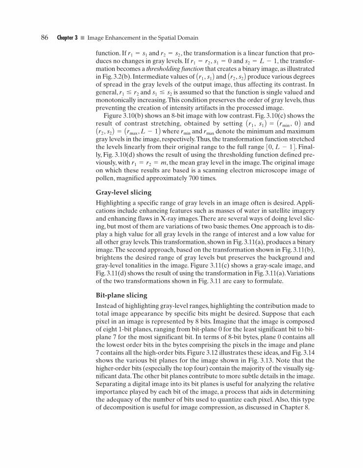
Figure 3.10(b) shows an 8-bit image with low contrast. Fig. 3.10(c) shows theresult of contrast stretching, obtained by setting Ar1 , s1 B= Armin , 0 B andAr2, s2 B=Armax, L-1B where rmin and rmax denote the minimum and maximumgray levels in the image, respectively.Thus, the transformation function stretchedthe levels linearly from their original range to the full range [0, L-1]. Final-ly, Fig. 3.10(d) shows the result of using the thresholding function defined pre-viously, with r1=r2=m, the mean gray level in the image.The original imageon which these results are based is a scanning electron microscope image ofpollen, magnified approximately 700 times.
Gray-level slicing
Highlighting a specific range of gray levels in an image often is desired. Appli-cations include enhancing features such as masses of water in satellite imageryand enhancing flaws in X-ray images.There are several ways of doing level slic-ing, but most of them are variations of two basic themes. One approach is to dis-play a high value for all gray levels in the range of interest and a low value forall other gray levels.This transformation, shown in Fig. 3.11(a), produces a binaryimage.The second approach, based on the transformation shown in Fig. 3.11(b),brightens the desired range of gray levels but preserves the background andgray-level tonalities in the image. Figure 3.11(c) shows a gray-scale image, andFig. 3.11(d) shows the result of using the transformation in Fig. 3.11(a).Variationsof the two transformations shown in Fig. 3.11 are easy to formulate.
Bit-plane slicing
Instead of highlighting gray-level ranges, highlighting the contribution made tototal image appearance by specific bits might be desired. Suppose that eachpixel in an image is represented by 8 bits. Imagine that the image is composedof eight 1-bit planes, ranging from bit-plane 0 for the least significant bit to bit-plane 7 for the most significant bit. In terms of 8-bit bytes, plane 0 contains allthe lowest order bits in the bytes comprising the pixels in the image and plane7 contains all the high-order bits. Figure 3.12 illustrates these ideas, and Fig. 3.14shows the various bit planes for the image shown in Fig. 3.13. Note that thehigher-order bits (especially the top four) contain the majority of the visually sig-nificant data.The other bit planes contribute to more subtle details in the image.Separating a digital image into its bit planes is useful for analyzing the relativeimportance played by each bit of the image, a process that aids in determiningthe adequacy of the number of bits used to quantize each pixel. Also, this typeof decomposition is useful for image compression, as discussed in Chapter 8.
GONZ03-075-146.II 29-08-2001 13:42 Page 86

3.2 � Some Basic Gray Level Transformations 87
L-1
L-1
s
r
T(r)
0 A B
L-1
L-1
s
r
T(r)
0 A B
FIGURE 3.11(a) Thistransformationhighlights range[A, B] of graylevels and reducesall others to aconstant level.(b) Thistransformationhighlights range[A, B] butpreserves allother levels.(c) An image.(d) Result ofusing thetransformationin (a).
One 8-bit byte Bit-plane 7(most significant)
Bit-plane 0(least significant)
FIGURE 3.12Bit-planerepresentation ofan 8-bit image.
In terms of bit-plane extraction for an 8-bit image, it is not difficult to showthat the (binary) image for bit-plane 7 can be obtained by processing the inputimage with a thresholding gray-level transformation function that (1) maps alllevels in the image between 0 and 127 to one level (for example, 0); and (2) mapsall levels between 129 and 255 to another (for example, 255).The binary imagefor bit-plane 7 in Fig. 3.14 was obtained in just this manner. It is left as an exer-cise (Problem 3.3) to obtain the gray-level transformation functions that wouldyield the other bit planes.
a bc d
GONZ03-075-146.II 29-08-2001 13:42 Page 87
88 Chapter 3 � Image Enhancement in the Spatial Domain
Histogram Processing
The histogram of a digital image with gray levels in the range [0, L-1] is a dis-crete function h Ark B=nk , where rk is the kth gray level and nk is the numberof pixels in the image having gray level rk . It is common practice to normalizea histogram by dividing each of its values by the total number of pixels in theimage, denoted by n. Thus, a normalized histogram is given by p Ark B=nk�n,for k=0, 1, p , L-1. Loosely speaking, p Ark B gives an estimate of the prob-ability of occurrence of gray level rk . Note that the sum of all components of anormalized histogram is equal to 1.
Histograms are the basis for numerous spatial domain processing techniques.Histogram manipulation can be used effectively for image enhancement, asshown in this section. In addition to providing useful image statistics, we shallsee in subsequent chapters that the information inherent in histograms also isquite useful in other image processing applications, such as image compressionand segmentation. Histograms are simple to calculate in software and also lendthemselves to economic hardware implementations, thus making them a pop-ular tool for real-time image processing.
As an introduction to the role of histogram processing in image enhance-ment, consider Fig. 3.15, which is the pollen image of Fig. 3.10 shown in fourbasic gray-level characteristics: dark, light, low contrast, and high contrast. Theright side of the figure shows the histograms corresponding to these images.The horizontal axis of each histogram plot corresponds to gray level values, rk .The vertical axis corresponds to values of h Ark B=nk or p Ark B=nk�n if thevalues are normalized. Thus, as indicated previously, these histogram plots aresimply plots of h Ark B=nk versus rk or p Ark B=nk�n versus rk .
3.3
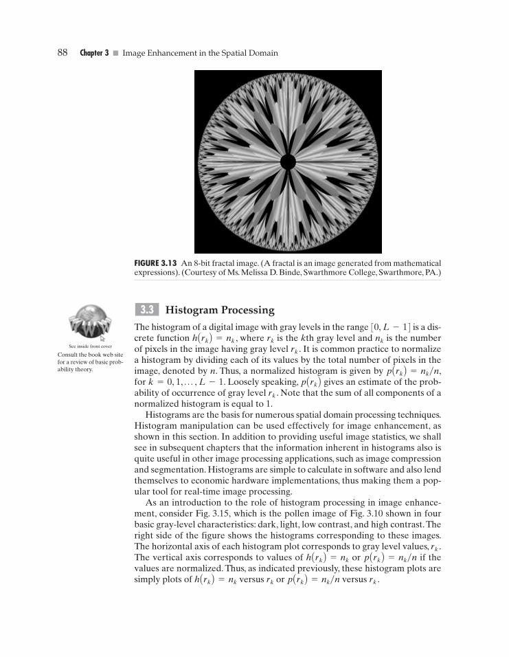
FIGURE 3.13 An 8-bit fractal image. (A fractal is an image generated from mathematicalexpressions). (Courtesy of Ms. Melissa D. Binde, Swarthmore College, Swarthmore, PA.)
Consult the book web sitefor a review of basic prob-ability theory.
See inside front cover
GONZ03-075-146.II 29-08-2001 13:42 Page 88

3.3 � Histogram Processing 89
FIGURE 3.14 The eight bit planes of the image in Fig. 3.13. The number at the bottom,right of each image identifies the bit plane.
We note in the dark image that the components of the histogram are con-centrated on the low (dark) side of the gray scale. Similarly, the components ofthe histogram of the bright image are biased toward the high side of the grayscale. An image with low contrast has a histogram that will be narrow and willbe centered toward the middle of the gray scale. For a monochrome image thisimplies a dull, washed-out gray look. Finally, we see that the components of thehistogram in the high-contrast image cover a broad range of the gray scale and,further, that the distribution of pixels is not too far from uniform, with very fewvertical lines being much higher than the others. Intuitively, it is reasonable toconclude that an image whose pixels tend to occupy the entire range of possi-ble gray levels and, in addition, tend to be distributed uniformly, will have an ap-pearance of high contrast and will exhibit a large variety of gray tones.The neteffect will be an image that shows a great deal of gray-level detail and has highdynamic range. It will be shown shortly that it is possible to develop a trans-formation function that can automatically achieve this effect, based only oninformation available in the histogram of the input image.
GONZ03-075-146.II 29-08-2001 13:42 Page 89

90 Chapter 3 � Image Enhancement in the Spatial Domain
Dark image
Bright image
Low-contrast image
High-contrast image
FIGURE 3.15 Four basic image types: dark, light, low contrast, high contrast, and their cor-responding histograms. (Original image courtesy of Dr. Roger Heady, Research Schoolof Biological Sciences, Australian National University, Canberra, Australia.)
a b
GONZ03-075-146.II 29-08-2001 13:42 Page 90
3.3 � Histogram Processing 91
3.3.1 Histogram EqualizationConsider for a moment continuous functions, and let the variable r represent thegray levels of the image to be enhanced. In the initial part of our discussion weassume that r has been normalized to the interval [0, 1], with r=0 represent-ing black and r=1 representing white. Later, we consider a discrete formula-tion and allow pixel values to be in the interval [0, L-1].
For any r satisfying the aforementioned conditions, we focus attention ontransformations of the form
s=T(r) 0 � r � 1 (3.3-1)
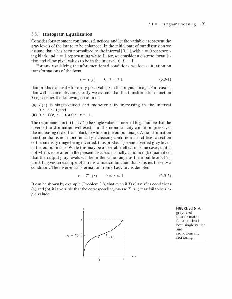
that produce a level s for every pixel value r in the original image. For reasonsthat will become obvious shortly, we assume that the transformation functionT(r) satisfies the following conditions:
(a) T(r) is single-valued and monotonically increasing in the interval0 � r � 1; and
(b) 0 � T(r) � 1 for 0 � r � 1.
The requirement in (a) that T(r) be single valued is needed to guarantee that theinverse transformation will exist, and the monotonicity condition preservesthe increasing order from black to white in the output image.A transformationfunction that is not monotonically increasing could result in at least a sectionof the intensity range being inverted, thus producing some inverted gray levelsin the output image. While this may be a desirable effect in some cases, that isnot what we are after in the present discussion. Finally, condition (b) guaranteesthat the output gray levels will be in the same range as the input levels. Fig-ure 3.16 gives an example of a transformation function that satisfies these twoconditions. The inverse transformation from s back to r is denoted
(3.3-2)
It can be shown by example (Problem 3.8) that even if T(r) satisfies conditions(a) and (b), it is possible that the corresponding inverse may fail to be sin-gle valued.
T-1(s)
r = T-1(s) 0 � s � 1.
T(r)
0 rk 1
t
r
s
sk=T(rk)
FIGURE 3.16 Agray-leveltransformationfunction that isboth single valuedandmonotonicallyincreasing.
GONZ03-075-146.II 29-08-2001 13:42 Page 91

92 Chapter 3 � Image Enhancement in the Spatial Domain
The gray levels in an image may be viewed as random variables in the in-terval [0, 1]. One of the most fundamental descriptors of a random variable isits probability density function (PDF). Let pr(r) and ps(s) denote the probabilitydensity functions of random variables r and s, respectively, where the subscriptson p are used to denote that pr and ps are different functions. A basic resultfrom an elementary probability theory is that, if pr(r) and T(r) are known and
satisfies condition (a), then the probability density function ps(s) of thetransformed variable s can be obtained using a rather simple formula:
(3.3-3)
Thus, the probability density function of the transformed variable, s, is deter-mined by the gray-level PDF of the input image and by the chosen transfor-mation function.
A transformation function of particular importance in image processinghas the form
(3.3-4)
where w is a dummy variable of integration.The right side of Eq. (3.3-4) is rec-ognized as the cumulative distribution function (CDF) of random variable r.Since probability density functions are always positive, and recalling that the in-tegral of a function is the area under the function, it follows that this transfor-mation function is single valued and monotonically increasing, and, therefore,satisfies condition (a). Similarly, the integral of a probability density function forvariables in the range [0, 1] also is in the range [0, 1], so condition (b) is satis-fied as well.
Given transformation function T(r), we find ps(s) by applying Eq. (3.3-3).Weknow from basic calculus (Leibniz’s rule) that the derivative of a definite inte-gral with respect to its upper limit is simply the integrand evaluated at that limit.In other words,
(3.3-5)
Substituting this result for dr�ds into Eq. (3.3-3), and keeping in mind that allprobability values are positive, yields
(3.3-6)
= 1 0 � s � 1.
= pr(r) 2 1pr(r)2
ps(s) = pr(r) 2 drds2
= pr(r).
=d
dr c 3
r
0pr(w) dw d
dsdr
=dT(r)
dr
s = T(r) = 3r
0pr(w) dw
ps(s) = pr(r) 2 drds2 .
T-1(s)
GONZ03-075-146.II 29-08-2001 13:42 Page 92

3.3 � Histogram Processing 93
Because ps(s) is a probability density function, it follows that it must be zero out-side the interval [0, 1] in this case because its integral over all values of s mustequal 1. We recognize the form of ps(s) given in Eq. (3.3-6) as a uniform prob-ability density function. Simply stated, we have demonstrated that performingthe transformation function given in Eq. (3.3-4) yields a random variable s char-acterized by a uniform probability density function. It is important to note fromEq. (3.3-4) that T(r) depends on pr(r), but, as indicated by Eq. (3.3-6), the re-sulting ps(s) always is uniform, independent of the form of pr(r).
For discrete values we deal with probabilities and summations instead ofprobability density functions and integrals. The probability of occurrence ofgray level rk in an image is approximated by
(3.3-7)
where, as noted at the beginning of this section, n is the total number of pixelsin the image, nk is the number of pixels that have gray level rk , and L is the totalnumber of possible gray levels in the image. The discrete version of the trans-formation function given in Eq. (3.3-4) is
(3.3-8)
Thus, a processed (output) image is obtained by mapping each pixel with levelrk in the input image into a corresponding pixel with level sk in the output imagevia Eq. (3.3-8). As indicated earlier, a plot of pr Ark B versus rk is called a his-togram. The transformation (mapping) given in Eq. (3.3-8) is called histogramequalization or histogram linearization. It is not difficult to show (Problem 3.9)that the transformation in Eq. (3.3-8) satisfies conditions (a) and (b) stated pre-viously in this section.
Unlike its continuos counterpart, it cannot be proved in general that this dis-crete transformation will produce the discrete equivalent of a uniform proba-bility density function, which would be a uniform histogram. However, as willbe seen shortly, use of Eq. (3.3-8) does have the general tendency of spreadingthe histogram of the input image so that the levels of the histogram-equalizedimage will span a fuller range of the gray scale.
We discussed earlier in this section the many advantages of having gray-levelvalues that cover the entire gray scale. In addition to producing gray levels thathave this tendency, the method just derived has the additional advantage thatit is fully “automatic.” In other words, given an image, the process of histogramequalization consists simply of implementing Eq. (3.3-8), which is based on in-formation that can be extracted directly from the given image, without the needfor further parameter specifications. We note also the simplicity of the compu-tations that would be required to implement the technique.
The inverse transformation from s back to r is denoted by
(3.3-9)rk = T-1AskB k = 0, 1, 2, p , L - 1
= ak
j = 0 nj
n k = 0, 1, 2, p , L - 1.
sk = TArkB = ak
j = 0prArjB
pr(rk) =nk
n k = 0, 1, 2, p , L - 1
GONZ03-075-146.II 29-08-2001 13:42 Page 93

94 Chapter 3 � Image Enhancement in the Spatial Domain
It can be shown (Problem 3.9) that the inverse transformation in Eq. (3.3-9)satisfies conditions (a) and (b) stated previously in this section only if none ofthe levels, rk , k=0, 1, 2, p , L-1, are missing from the input image.Althoughthe inverse transformation is not used in histogram equalization, it plays a cen-tral role in the histogram-matching scheme developed in the next section. Wealso discuss in that section details of how to implement histogram processingtechniques.
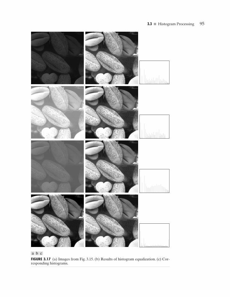
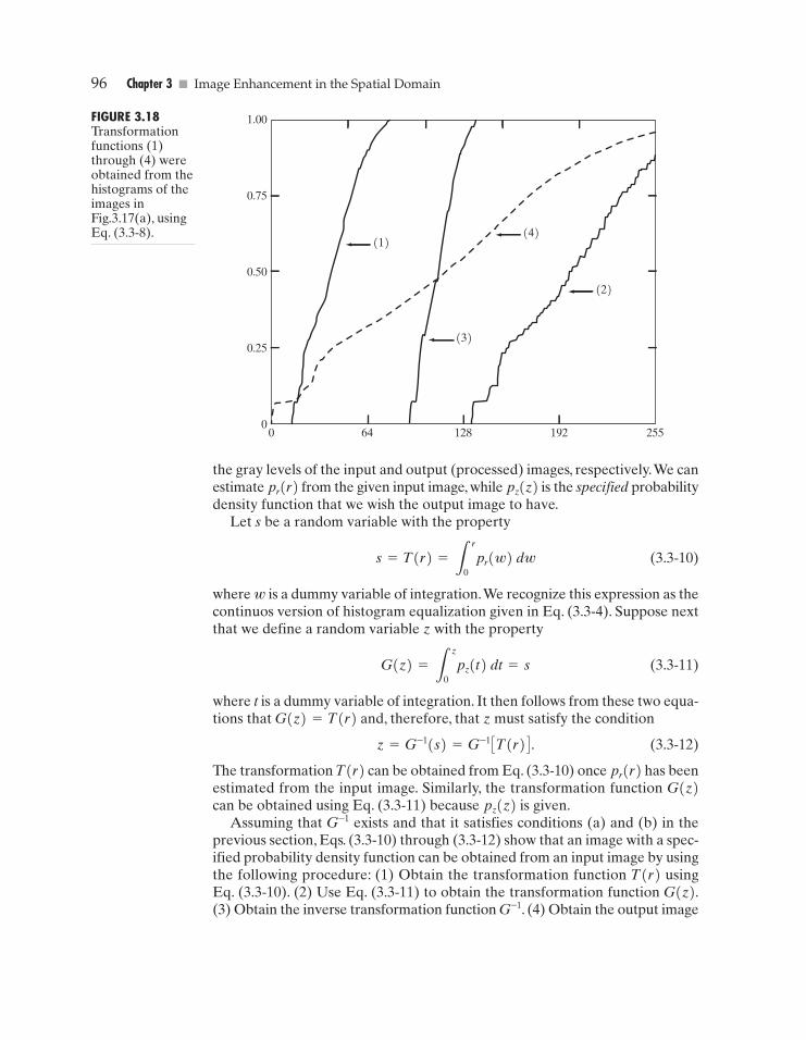
� Figure 3.17(a) shows the four images from Fig. 3.15, and Fig. 3.17(b) showsthe result of performing histogram equalization on each of these images.The firstthree results (top to bottom) show significant improvement. As expected, his-togram equalization did not produce a significant visual difference in the fourthimage because the histogram of this image already spans the full spectrum ofthe gray scale. The transformation functions used to generate the images inFig. 3.17(b) are shown in Fig. 3.18. These functions were generated from thehistograms of the original images [see Fig. 3.15(b)] using Eq. (3.3-8). Note thattransformation (4) has a basic linear shape, again indicating that the gray lev-els in the fourth input image are nearly uniformly distributed.As was just noted,we would expect histogram equalization in this case to have negligible effect onthe appearance of the image.
The histograms of the equalized images are shown in Fig. 3.17(c). It is of in-terest to note that, while all these histograms are different, the histogram-equalized images themselves are visually very similar. This is not unexpectedbecause the difference between the images in the left column is simply one ofcontrast, not of content. In other words, since the images have the same content,the increase in contrast resulting from histogram equalization was enough torender any gray-level differences in the resulting images visually indistinguish-able. Given the significant contrast differences of the images in the left column,this example illustrates the power of histogram equalization as an adaptive en-hancement tool. �
3.3.2 Histogram Matching (Specification)As indicated in the preceding discussion, histogram equalization automatical-ly determines a transformation function that seeks to produce an output imagethat has a uniform histogram. When automatic enhancement is desired, this isa good approach because the results from this technique are predictable and themethod is simple to implement. We show in this section that there are applica-tions in which attempting to base enhancement on a uniform histogram is notthe best approach. In particular, it is useful sometimes to be able to specify theshape of the histogram that we wish the processed image to have. The methodused to generate a processed image that has a specified histogram is calledhistogram matching or histogram specification.
Development of the method
Let us return for a moment to continuous gray levels r and z (consideredcontinuous random variables), and let pr(r) and pz(z) denote their corre-sponding continuos probability density functions. In this notation, r and z denote
EXAMPLE 3.3:Histogramequalization.
GONZ03-075-146.II 29-08-2001 13:42 Page 94
3.3 � Histogram Processing 95
FIGURE 3.17 (a) Images from Fig. 3.15. (b) Results of histogram equalization. (c) Cor-responding histograms.
a b c
GONZ03-075-146.II 29-08-2001 13:42 Page 95
96 Chapter 3 � Image Enhancement in the Spatial Domain
1.00
0.75
0.50
0.25
00 64
(1)
(3)
(2)
(4)
128 192 255
FIGURE 3.18Transformationfunctions (1)through (4) wereobtained from thehistograms of theimages inFig.3.17(a), usingEq. (3.3-8).
the gray levels of the input and output (processed) images, respectively.We canestimate pr(r) from the given input image, while pz(z) is the specified probabilitydensity function that we wish the output image to have.
Let s be a random variable with the property
(3.3-10)
where w is a dummy variable of integration.We recognize this expression as thecontinuos version of histogram equalization given in Eq. (3.3-4). Suppose nextthat we define a random variable z with the property
(3.3-11)
where t is a dummy variable of integration. It then follows from these two equa-tions that G(z)=T(r) and, therefore, that z must satisfy the condition
(3.3-12)
The transformation T(r) can be obtained from Eq. (3.3-10) once pr(r) has beenestimated from the input image. Similarly, the transformation function G(z)can be obtained using Eq. (3.3-11) because pz(z) is given.
Assuming that G–1 exists and that it satisfies conditions (a) and (b) in theprevious section, Eqs. (3.3-10) through (3.3-12) show that an image with a spec-ified probability density function can be obtained from an input image by usingthe following procedure: (1) Obtain the transformation function T(r) usingEq. (3.3-10). (2) Use Eq. (3.3-11) to obtain the transformation function G(z).(3) Obtain the inverse transformation function G–1. (4) Obtain the output image
z = G-1(s) = G-1 CT(r) D .
G(z) = 3z
0pz(t) dt = s
s = T(r) = 3r
0pr(w) dw
GONZ03-075-146.II 29-08-2001 13:42 Page 96

3.3 � Histogram Processing 97
by applying Eq. (3.3-12) to all the pixels in the input image.The result of this pro-cedure will be an image whose gray levels, z, have the specified probability den-sity function pz(z).
Although the procedure just described is straightforward in principle, it isseldom possible in practice to obtain analytical expressions for T(r) and forG–1. Fortunately, this problem is simplified considerably in the case of discretevalues.The price we pay is the same as in histogram equalization, where only anapproximation to the desired histogram is achievable. In spite of this, however,some very useful results can be obtained even with crude approximations.
The discrete formulation of Eq. (3.3-10) is given by Eq. (3.3-8), which we re-peat here for convenience:
(3.3-13)
where n is the total number of pixels in the image, nj is the number of pixels withgray level rj , and L is the number of discrete gray levels. Similarly, the discreteformulation of Eq. (3.3-11) is obtained from the given histogram pz Azi B , i=0,1, 2, p , L-1, and has the form
(3.3-14)
As in the continuos case, we are seeking values of z that satisfy this equation.The variable vk was added here for clarity in the discussion that follows. Final-ly, the discrete version of Eq. (3.3-12) is given by
(3.3-15)
or, from Eq. (3.3-13),
(3.3-16)
Equations (3.3-13) through (3.3-16) are the foundation for implementinghistogram matching for digital images. Equation (3.3-13) is a mapping from thelevels in the original image into corresponding levels sk based on the histogramof the original image, which we compute from the pixels in the image. Equation(3.3-14) computes a transformation function G from the given histogram pz(z).Finally, Eq. (3.3-15) or its equivalent, Eq. (3.3-16), gives us (an approximationof) the desired levels of the image with that histogram. The first two equationscan be implemented easily because all the quantities are known. Implementa-tion of Eq. (3.3-16) is straightforward, but requires additional explanation.
Implementation
We start by noting the following: (1) Each set of gray levels ErjF , EsjF , and EzjF ,j=0, 1, 2, p , L-1, is a one-dimensional array of dimension L*1. (2) Allmappings from r to s and from s to z are simple table lookups between a given
zk = G-1AskB k = 0, 1, 2, p , L - 1.
zk = G-1 CTArkB D k = 0, 1, 2, p , L - 1
vk = GAzkB = ak
i = 0pzAziB = sk k = 0, 1, 2, p , L - 1.
= ak
j = 0 nj
n k = 0, 1, 2, p , L - 1
sk = TArkB = a k
j = 0prArjB
GONZ03-075-146.II 29-08-2001 13:42 Page 97

98 Chapter 3 � Image Enhancement in the Spatial Domain
0 L-10
s
r
1
rk
sk
T(r)
L-1
v
z0 zq
vq
0
1
G(z)
L-1
v
z0 zk
sk
0
1
G(z)
FIGURE 3.19(a) Graphicalinterpretation ofmapping from rk
to sk via T(r).(b) Mapping of zq
to itscorrespondingvalue vq via G(z).(c) Inversemapping from sk
to itscorrespondingvalue of zk .
a bc
pixel value and these arrays. (3) Each of the elements of these arrays, for ex-ample, sk , contains two important pieces of information: The subscript k de-notes the location of the element in the array, and s denotes the value at thatlocation. (4) We need to be concerned only with integer pixel values. For ex-ample, in the case of an 8-bit image, L=256 and the elements of each of thearrays just mentioned are integers between 0 and 255.This implies that we nowwork with gray level values in the interval [0, L-1] instead of the normalizedinterval [0, 1] that we used before to simplify the development of histogramprocessing techniques.
In order to see how histogram matching actually can be implemented, con-sider Fig. 3.19(a), ignoring for a moment the connection shown between thisfigure and Fig. 3.19(c). Figure 3.19(a) shows a hypothetical discrete transfor-mation function s=T(r) obtained from a given image. The first gray level inthe image, r1 , maps to s1 ; the second gray level, r2 , maps to s2 ; the kth level rk
maps to sk ; and so on (the important point here is the ordered correspondencebetween these values). Each value sj in the array is precomputed usingEq. (3.3-13), so the process of mapping simply uses the actual value of a pixelas an index in an array to determine the corresponding value of s. This processis particularly easy because we are dealing with integers. For example, the smapping for an 8-bit pixel with value 127 would be found in the 128th positionin array EsjF (recall that we start at 0) out of the possible 256 positions. If westopped here and mapped the value of each pixel of an input image by the
GONZ03-075-146.II 29-08-2001 13:42 Page 98

3.3 � Histogram Processing 99
method just described, the output would be a histogram-equalized image, ac-cording to Eq. (3.3-8).
In order to implement histogram matching we have to go one step further.Figure 3.19(b) is a hypothetical transformation function G obtained from agiven histogram pz(z) by using Eq. (3.3-14). For any zq , this transformationfunction yields a corresponding value vq . This mapping is shown by the arrowsin Fig. 3.19(b). Conversely, given any value vq , we would find the correspond-ing value zq from G–1. In terms of the figure, all this means graphically is that wewould reverse the direction of the arrows to map vq into its corresponding zq .However, we know from the definition in Eq. (3.3-14) that v=s for corre-sponding subscripts, so we can use exactly this process to find the zk corre-sponding to any value sk that we computed previously from the equationsk=T Ark B . This idea is shown in Fig. 3.19(c).
Since we really do not have the z’s (recall that finding these values is pre-cisely the objective of histogram matching), we must resort to some sort of iter-ative scheme to find z from s. The fact that we are dealing with integers makesthis a particularly simple process. Basically, because vk=sk , we have fromEq. (3.3-14) that the z’s for which we are looking must satisfy the equationGAzk B=sk , or AGAzk B-skB=0. Thus, all we have to do to find the value of zk
corresponding to sk is to iterate on values of z such that this equation is satisfiedfor k=0, 1, 2, p , L-1. This is the same thing as Eq. (3.3-16), except that wedo not have to find the inverse of G because we are going to iterate on z. Sincewe are dealing with integers, the closest we can get to satisfying the equationAG Azk B-sk B=0 is to let zk= for each value of k, where is the smallestinteger in the interval [0, L-1] such that
(3.3-17)
Given a value sk , all this means conceptually in terms of Fig. 3.19(c) is that wewould start with and increase it in integer steps until Eq. (3.3-17) is sat-isfied, at which point we let Repeating this process for all values of kwould yield all the required mappings from s to z, which constitutes the im-plementation of Eq. (3.3-16). In practice, we would not have to start witheach time because the values of sk are known to increase monotonically. Thus,for k=k+1, we would start with and increment in integer valuesfrom there.
The procedure we have just developed for histogram matching may be sum-marized as follows:
1. Obtain the histogram of the given image.2. Use Eq. (3.3-13) to precompute a mapped level sk for each level rk .3. Obtain the transformation function G from the given pz(z) using
Eq. (3.3-14).4. Precompute zk for each value of sk using the iterative scheme defined in con-
nection with Eq. (3.3-17).5. For each pixel in the original image, if the value of that pixel is rk , map this
value to its corresponding level sk ; then map level sk into the final level zk .Use the precomputed values from Steps (2) and (4) for these mappings.
z = zk
z = 0
zk = z.z = 0
AG(z) - skB � 0 k = 0, 1, 2, p , L - 1.
zz
GONZ03-075-146.II 29-08-2001 13:42 Page 99
100 Chapter 3 � Image Enhancement in the Spatial Domain
7.00
5.25
3.50
1.75
00 64 128 192 255
Gray level
Num
ber
of p
ixel
s (*
104 )
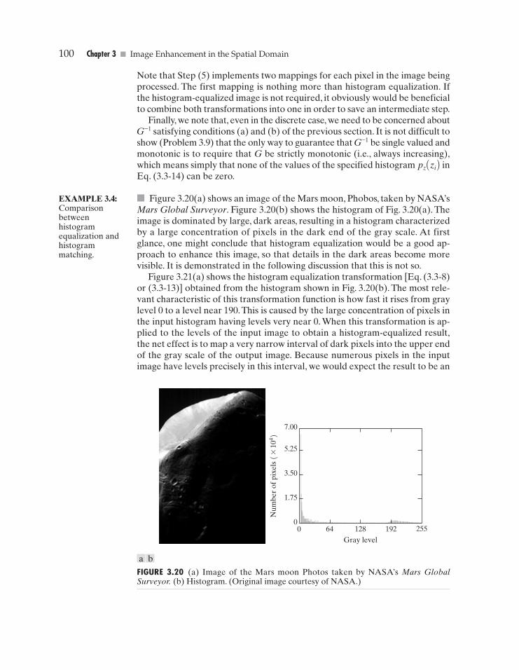
FIGURE 3.20 (a) Image of the Mars moon Photos taken by NASA’s Mars GlobalSurveyor. (b) Histogram. (Original image courtesy of NASA.)
Note that Step (5) implements two mappings for each pixel in the image beingprocessed. The first mapping is nothing more than histogram equalization. Ifthe histogram-equalized image is not required, it obviously would be beneficialto combine both transformations into one in order to save an intermediate step.
Finally, we note that, even in the discrete case, we need to be concerned aboutG–1 satisfying conditions (a) and (b) of the previous section. It is not difficult toshow (Problem 3.9) that the only way to guarantee that G–1 be single valued andmonotonic is to require that G be strictly monotonic (i.e., always increasing),which means simply that none of the values of the specified histogram pz Azi B inEq. (3.3-14) can be zero.
� Figure 3.20(a) shows an image of the Mars moon, Phobos, taken by NASA’sMars Global Surveyor. Figure 3.20(b) shows the histogram of Fig. 3.20(a). Theimage is dominated by large, dark areas, resulting in a histogram characterizedby a large concentration of pixels in the dark end of the gray scale. At firstglance, one might conclude that histogram equalization would be a good ap-proach to enhance this image, so that details in the dark areas become morevisible. It is demonstrated in the following discussion that this is not so.
Figure 3.21(a) shows the histogram equalization transformation [Eq. (3.3-8)or (3.3-13)] obtained from the histogram shown in Fig. 3.20(b). The most rele-vant characteristic of this transformation function is how fast it rises from graylevel 0 to a level near 190.This is caused by the large concentration of pixels inthe input histogram having levels very near 0. When this transformation is ap-plied to the levels of the input image to obtain a histogram-equalized result,the net effect is to map a very narrow interval of dark pixels into the upper endof the gray scale of the output image. Because numerous pixels in the inputimage have levels precisely in this interval, we would expect the result to be an
EXAMPLE 3.4:Comparisonbetweenhistogramequalization andhistogrammatching.
a b
GONZ03-075-146.II 29-08-2001 13:42 Page 100

3.3 � Histogram Processing 101
255
192
128
64
00 64 128 192 255
Input gray levels
Out
put g
ray
leve
ls
7.00
5.25
3.50
1.75
00 64 128 192 255
Gray level
Num
ber
of p
ixel
s (*
104 )
FIGURE 3.21(a) Transformationfunction forhistogramequalization.(b) Histogram-equalized image(note the washed-out appearance).(c) Histogram of (b).
image with a light, washed-out appearance. As shown in Fig. 3.21(b), this is in-deed the case.The histogram of this image is shown in Fig. 3.21(c). Note how allthe gray levels are biased toward the upper one-half of the gray scale.
Since the problem with the transformation function in Fig. 3.21(a) was causedby a large concentration of pixels in the original image with levels near 0, a rea-sonable approach is to modify the histogram of that image so that it does nothave this property. Figure 3.22(a) shows a manually specified function that pre-serves the general shape of the original histogram, but has a smoother transitionof levels in the dark region of the gray scale. Sampling this function into 256equally spaced discrete values produced the desired specified histogram. Thetransformation function G(z) obtained from this histogram using Eq. (3.3-14) islabeled transformation (1) in Fig. 3.22(b). Similarly, the inverse transformationG–1(s) from Eq. (3.3-16) [obtained using the iterative technique discussed inconnection with Eq. (3.3-17)] is labeled transformation (2) in Fig. 3.22(b).The en-hanced image in Fig. 3.22(c) was obtained by applying transformation (2) to thepixels of the histogram-equalized image in Fig. 3.21(b).The improvement of thehistogram-specified image over the result obtained by histogram equalization isevident by comparing these two images. It is of interest to note that a rathermodest change in the original histogram was all that was required to obtain a sig-nificant improvement in enhancement.The histogram of Fig. 3.22(c) is shown inFig. 3.22(d).The most distinguishing feature of this histogram is how its low endhas shifted right toward the lighter region of the gray scale, as desired. �
a bc
GONZ03-075-146.II 29-08-2001 13:42 Page 101

102 Chapter 3 � Image Enhancement in the Spatial Domain
7.00
5.25
3.50
1.75
00 64 128 192 255
Gray level
Num
ber
of p
ixel
s (*
104 )
255
192
128
64
00 64 128 192 255
Input gray levels
Out
put g
ray
leve
ls
(2)
(1)
7.00
5.25
3.50
1.75
00 64 128 192 255
Gray level
Num
ber
of p
ixel
s (*
104 )
FIGURE 3.22(a) Specifiedhistogram.(b) Curve (1) isfrom Eq. (3.3-14),using thehistogram in (a);curve (2) wasobtained usingthe iterativeprocedure inEq. (3.3-17).(c) Enhancedimage usingmappings fromcurve (2).(d) Histogram of (c).
Although it probably is obvious by now, we emphasize before leaving this sec-tion that histogram specification is, for the most part, a trial-and-error process.One can use guidelines learned from the problem at hand, just as we did in thepreceding example. At times, there may be cases in which it is possible to for-mulate what an “average” histogram should look like and use that as the spec-ified histogram. In cases such as these, histogram specification becomes astraightforward process. In general, however, there are no rules for specifyinghistograms, and one must resort to analysis on a case-by-case basis for any givenenhancement task.
a cbd
GONZ03-075-146.II 29-08-2001 13:42 Page 102

3.3 � Histogram Processing 103
3.3.3 Local EnhancementThe histogram processing methods discussed in the previous two sections areglobal, in the sense that pixels are modified by a transformation function basedon the gray-level content of an entire image. Although this global approach issuitable for overall enhancement, there are cases in which it is necessary to en-hance details over small areas in an image.The number of pixels in these areasmay have negligible influence on the computation of a global transformationwhose shape does not necessarily guarantee the desired local enhancement.The solution is to devise transformation functions based on the gray-level dis-tribution—or other properties—in the neighborhood of every pixel in the image.Although processing methods based on neighborhoods are the topic of Section3.5, we discuss local histogram processing here for the sake of clarity and con-tinuity. The reader will have no difficulty in following the discussion.
The histogram processing techniques previously described are easily adapt-able to local enhancement. The procedure is to define a square or rectangularneighborhood and move the center of this area from pixel to pixel. At each lo-cation, the histogram of the points in the neighborhood is computed and eithera histogram equalization or histogram specification transformation function isobtained. This function is finally used to map the gray level of the pixel cen-tered in the neighborhood.The center of the neighborhood region is then movedto an adjacent pixel location and the procedure is repeated. Since only one newrow or column of the neighborhood changes during a pixel-to-pixel translationof the region, updating the histogram obtained in the previous location withthe new data introduced at each motion step is possible (Problem 3.11).This ap-proach has obvious advantages over repeatedly computing the histogram overall pixels in the neighborhood region each time the region is moved one pixellocation.Another approach used some times to reduce computation is to utilizenonoverlapping regions, but this method usually produces an undesirablecheckerboard effect.
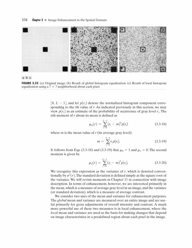
� Figure 3.23(a) shows an image that has been slightly blurred to reduce itsnoise content (see Section 3.6.1 regarding blurring). Figure 3.23(b) shows the re-sult of global histogram equalization. As is often the case when this techniqueis applied to smooth, noisy areas, Fig. 3.23(b) shows considerable enhancementof the noise, with a slight increase in contrast. Note that no new structural de-tails were brought out by this method. However, local histogram equalizationusing a 7*7 neighborhood revealed the presence of small squares inside thelarger dark squares. The small squares were too close in gray level to the larg-er ones, and their sizes were too small to influence global histogram equaliza-tion significantly. Note also the finer noise texture in Fig. 3.23(c), a result oflocal processing using relatively small neighborhoods. �
3.3.4 Use of Histogram Statistics for Image EnhancementInstead of using the image histogram directly for enhancement, we can use in-stead some statistical parameters obtainable directly from the histogram. Let rdenote a discrete random variable representing discrete gray-levels in the range
EXAMPLE 3.5:Enhancementusing localhistograms.
GONZ03-075-146.II 29-08-2001 13:42 Page 103
104 Chapter 3 � Image Enhancement in the Spatial Domain
FIGURE 3.23 (a) Original image. (b) Result of global histogram equalization. (c) Result of local histogramequalization using a 7*7 neighborhood about each pixel.
[0, L-1], and let p Ari B denote the normalized histogram component corre-sponding to the ith value of r. As indicated previously in this section, we mayview p Ari B as an estimate of the probability of occurrence of gray level ri . Thenth moment of r about its mean is defined as
(3.3-18)
where m is the mean value of r (its average gray level):
(3.3-19)
It follows from Eqs. (3.3-18) and (3.3-19) that m0=1 and m1=0. The secondmoment is given by
(3.3-20)
We recognize this expression as the variance of r, which is denoted conven-tionally by s2(r).The standard deviation is defined simply as the square root ofthe variance. We will revisit moments in Chapter 11 in connection with imagedescription. In terms of enhancement, however, we are interested primarily inthe mean, which is a measure of average gray level in an image, and the variance(or standard deviation), which is a measure of average contrast.
We consider two uses of the mean and variance for enhancement purposes.The global mean and variance are measured over an entire image and are use-ful primarily for gross adjustments of overall intensity and contrast. A muchmore powerful use of these two measures is in local enhancement, where thelocal mean and variance are used as the basis for making changes that dependon image characteristics in a predefined region about each pixel in the image.
m2(r) = aL - 1
i = 0Ari - mB2pAriB.
m = aL - 1
i = 0ri pAriB.
mn(r) = aL - 1
i = 0Ari - mBnpAriB
a b c
GONZ03-075-146.II 29-08-2001 13:42 Page 104

3.3 � Histogram Processing 105
Let (x, y) be the coordinates of a pixel in an image, and let Sxy denote aneighborhood (subimage) of specified size, centered at (x, y). From Eq. (3.3-19)the mean value of the pixels in Sxy can be computed using the expression
(3.3-21)
where rs, t is the gray level at coordinates (s, t) in the neighborhood, and p Ars, t Bis the neighborhood normalized histogram component corresponding to thatvalue of gray level. Similarly, from Eq. (3.3-20), the gray-level variance of the pix-els in region Sxy is given by
(3.3-22)
The local mean is a measure of average gray level in neighborhood Sxy , and thevariance (or standard deviation) is a measure of contrast in that neighborhood.
An important aspect of image processing using the local mean and varianceis the flexibility they afford in developing simple, yet powerful enhancementtechniques based on statistical measures that have a close, predictable corre-spondence with image appearance.We illustrate these characteristics by meansof an example.
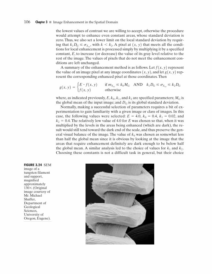
� Figure 3.24 shows an SEM (scanning electron microscope) image of a tung-sten filament wrapped around a support. The filament in the center of theimage and its support are quite clear and easy to study. There is another fila-ment structure on the right side of the image, but it is much darker and its sizeand other features are not as easily discernable. Local enhancement by contrastmanipulation is an ideal approach to try on problems such as this, where partof the image is acceptable, but other parts may contain hidden features of in-terest.
In this particular case, the problem is to enhance dark areas while leaving thelight area as unchanged as possible since it does note require enhancement.Wecan use the concepts presented in this section to formulate an enhancementmethod that can tell the difference between dark and light and, at the sametime, is capable of enhancing only the dark areas.A measure of whether an areais relatively light or dark at a point (x, y) is to compare the local average graylevel to the average image gray level, called the global mean and denotedMG . This latter quantity is obtained by letting S encompass the entire image.Thus, we have the first element of our enhancement scheme: We will considerthe pixel at a point (x, y) as a candidate for processing if wherek0 is a positive constant with value less than 1.0. Since we are interested in en-hancing areas that have low contrast, we also need a measure to determinewhether the contrast of an area makes it a candidate for enhancement.Thus, wewill consider the pixel at a point (x, y) as a candidate for enhancement if
where DG is the global standard deviation and k2 is a positive con-stant. The value of this constant will be greater than 1.0 if we are interested inenhancing light areas and less than 1.0 for dark areas. Finally, we need to restrict
sSxy� k2 DG ,
mSxy� k0 MG ,
mSxy
s2Sxy
= a
(s, t)HSxy
Crs, t - mSxyD 2pArs, tB.
mSxy= a
(s, t)HSxy
rs, t pArs, tBmSxy
EXAMPLE 3.6:Enhancementbased on localstatistics.
GONZ03-075-146.II 29-08-2001 13:42 Page 105
106 Chapter 3 � Image Enhancement in the Spatial Domain
the lowest values of contrast we are willing to accept, otherwise the procedurewould attempt to enhance even constant areas, whose standard deviation iszero. Thus, we also set a lower limit on the local standard deviation by requir-ing that with k<k2. A pixel at (x, y) that meets all the condi-tions for local enhancement is processed simply by multiplying it by a specifiedconstant, E, to increase (or decrease) the value of its gray level relative to therest of the image. The values of pixels that do not meet the enhancement con-ditions are left unchanged.
A summary of the enhancement method is as follows. Let f(x, y) representthe value of an image pixel at any image coordinates (x, y), and let g(x, y) rep-resent the corresponding enhanced pixel at those coordinates. Then
where, as indicated previously, E, k0 , k1 , and k2 are specified parameters; MG isthe global mean of the input image; and DG is its global standard deviation.
Normally, making a successful selection of parameters requires a bit of ex-perimentation to gain familiarity with a given image or class of images. In thiscase, the following values were selected: E=4.0, k0=0.4, k1=0.02, andk2=0.4. The relatively low value of 4.0 for E was chosen so that, when it wasmultiplied by the levels in the areas being enhanced (which are dark), the re-sult would still tend toward the dark end of the scale, and thus preserve the gen-eral visual balance of the image. The value of k0 was chosen as somewhat lessthan half the global mean since it is obvious by looking at the image that theareas that require enhancement definitely are dark enough to be below halfthe global mean. A similar analysis led to the choice of values for k1 and k2 .Choosing these constants is not a difficult task in general, but their choice
g(x, y) = bE � f(x, y)
f(x, y)
if mSxy� k0 MG AND k1 DG � sSxy
� k2 DG
otherwise
k1 DG � sSxy ,
FIGURE 3.24 SEMimage of atungsten filamentand support,magnifiedapproximately130*. (Originalimage courtesy ofMr. MichaelShaffer,Department ofGeologicalSciences,University ofOregon, Eugene).
GONZ03-075-146.II 29-08-2001 13:42 Page 106

3.3 � Histogram Processing 107
FIGURE 3.25 (a) Image formed from all local means obtained from Fig. 3.24 using Eq. (3.3-21). (b) Imageformed from all local standard deviations obtained from Fig. 3.24 using Eq. (3.3-22). (c) Image formed fromall multiplication constants used to produce the enhanced image shown in Fig. 3.26.
definitely must be guided by a logical analysis of the enhancement problem athand. Finally, the choice of size for the local area should be as small as possiblein order to preserve detail and keep the computational burden as low as possi-ble. We chose a small (3*3) local region.
Figure 3.25(a) shows the values of for all values of (x, y). Since the valueof for each (x, y) is the average of the neighboring pixels in a 3*3 areacentered at (x, y), we expect the result to be similar to the original image, but
mSxy
mSxy
a b c
FIGURE 3.26Enhanced SEMimage. Comparewith Fig. 3.24. Notein particular theenhanced area onthe right, bottomside of the image.
GONZ03-075-146.II 29-08-2001 13:42 Page 107

108 Chapter 3 � Image Enhancement in the Spatial Domain
slightly blurred. This indeed is the case in Fig. 3.25(a). Figure 3.25(b) shows inimage formed using all the values of Similarly, we can construct an imageout the values that multiply f(x, y) at each coordinate pair (x, y) to form g(x, y).Since the values are either 1 or E, the image is binary, as shown in Fig. 3.25(c).The dark areas correspond to 1 and the light areas to E.Thus, any light point inFig. 3.25(c) signifies a coordinate pair (x, y) at which the enhancement proce-dure multiplied f(x, y) by E to produce an enhanced pixel. The dark pointsrepresent coordinates at which the procedure did not to modify the pixel values.
The enhanced image obtained with the method just described is shown inFig.3.26. In comparing this image with the original in Fig.3.24,we note the obviousdetail that has been brought out on the right side of the enhanced image.It is worth-while to point out that the unenhanced portions of the image (the light areas) wereleft intact for the most part.We do note the appearance of some small bright dotsin the shadow areas where the coil meets the support stem,and around some of theborders between the filament and the background.These are undesirable artifactscreated by the enhancement technique.In other words,the points appearing as lightdots met the criteria for enhancement and their values were amplified by factor E.Introduction of artifacts is a definite drawback of a method such as the one just de-scribed because of the nonlinear way in which they process an image.The key pointhere, however, is that the image was enhanced in a most satisfactory way as far asbringing out the desired detail. �
It is not difficult to imagine the numerous ways in which the example justgiven could be adapted or extended to other situations in which local en-hancement is applicable.
Enhancement Using Arithmetic/Logic Operations
Arithmetic/logic operations involving images are performed on a pixel-by-pixelbasis between two or more images (this excludes the logic operation NOT, whichis performed on a single image). As an example, subtraction of two images re-sults in a new image whose pixel at coordinates (x, y) is the difference betweenthe pixels in that same location in the two images being subtracted. Dependingon the hardware and/or software being used, the actual mechanics of imple-menting arithmetic/logic operations can be done sequentially, one pixel at atime, or in parallel, where all operations are performed simultaneously.
Logic operations similarly operate on a pixel-by-pixel basis†. We need onlybe concerned with the ability to implement the AND, OR, and NOT logic op-erators because these three operators are functionally complete. In other words,any other logic operator can be implemented by using only these three basicfunctions.When dealing with logic operations on gray-scale images, pixel valuesare processed as strings of binary numbers. For example, performing the NOToperation on a black, 8-bit pixel (a string of eight 0’s) produces a white pixel
3.4
sSxy .
† Recall that, for two binary variables a and b: aANDb yields 1 only when both a and b are 1; otherwisethe result is 0. Similarly, aORb is 0 when both variables are 0; otherwise the result is 1. Finally, if a is 1,NOT (a) is 0, and vice versa.
GONZ03-075-146.II 29-08-2001 13:42 Page 108

3.4 � Enhancement Using Arithmetic/Logic Operations 109
FIGURE 3.27(a) Originalimage. (b) ANDimage mask.(c) Result of theAND operationon images (a) and(b). (d) Originalimage. (e) ORimage mask.(f) Result ofoperation OR onimages (d) and(e).
(a string of eight 1’s). Intermediate values are processed the same way, chang-ing all 1’s to 0’s and vice versa.Thus, the NOT logic operator performs the samefunction as the negative transformation of Eq. (3.2-1). The AND and OR op-erations are used for masking; that is, for selecting subimages in an image, as il-lustrated in Fig. 3.27. In the AND and OR image masks, light represents a binary1 and dark represents a binary 0. Masking sometimes is referred to as region ofinterest (ROI) processing. In terms of enhancement, masking is used primarilyto isolate an area for processing. This is done to highlight that area and differ-entiate it from the rest of the image. Logic operations also are used frequentlyin conjunction with morphological operations, as discussed in Chapter 9.
Of the four arithmetic operations, subtraction and addition (in that order) arethe most useful for image enhancement. We consider division of two imagessimply as multiplication of one image by the reciprocal of the other.Aside fromthe obvious operation of multiplying an image by a constant to increase its av-erage gray level, image multiplication finds use in enhancement primarily as amasking operation that is more general than the logical masks discussed in theprevious paragraph. In other words, multiplication of one image by another canbe used to implement gray-level, rather than binary, masks. We give an exam-ple in Section 3.8 of how such a masking operation can be a useful tool. In theremainder of this section, we develop and illustrate methods based on subtrac-tion and addition for image enhancement. Other uses of image multiplicationare discussed in Chapter 5, in the context of image restoration.
a b cd e f
GONZ03-075-146.II 29-08-2001 13:42 Page 109
110 Chapter 3 � Image Enhancement in the Spatial Domain
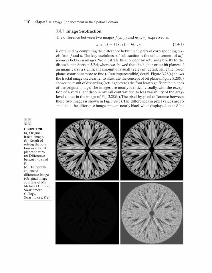
FIGURE 3.28(a) Originalfractal image.(b) Result ofsetting the fourlower-order bitplanes to zero.(c) Differencebetween (a) and(b).(d) Histogram-equalizeddifference image.(Original imagecourtesy of Ms.Melissa D. Binde,SwarthmoreCollege,Swarthmore, PA).
3.4.1 Image SubtractionThe difference between two images f(x, y) and h(x, y), expressed as
(3.4-1)
is obtained by computing the difference between all pairs of corresponding pix-els from f and h. The key usefulness of subtraction is the enhancement of dif-ferences between images. We illustrate this concept by returning briefly to thediscussion in Section 3.2.4, where we showed that the higher-order bit planes ofan image carry a significant amount of visually relevant detail, while the lowerplanes contribute more to fine (often imperceptible) detail. Figure 3.28(a) showsthe fractal image used earlier to illustrate the concept of bit planes. Figure 3.28(b)shows the result of discarding (setting to zero) the four least significant bit planesof the original image. The images are nearly identical visually, with the excep-tion of a very slight drop in overall contrast due to less variability of the gray-level values in the image of Fig. 3.28(b). The pixel-by-pixel difference betweenthese two images is shown in Fig. 3.28(c). The differences in pixel values are sosmall that the difference image appears nearly black when displayed on an 8-bit
g(x, y) = f(x, y) - h(x, y),
a bc d
GONZ03-075-146.II 29-08-2001 13:42 Page 110

3.4 � Enhancement Using Arithmetic/Logic Operations 111
display. In order to bring out more detail, we can perform a contrast stretchingtransformation, such as those discussed in Sections 3.2 or 3.3. We chose his-togram equalization, but an appropriate power-law transformation would havedone the job also.The result is shown in Fig. 3.28(d).This is a very useful imagefor evaluating the effect of setting to zero the lower-order planes.
� One of the most commercially successful and beneficial uses of image sub-traction is in the area of medical imaging called mask mode radiography. In thiscase h(x, y), the mask, is an X-ray image of a region of a patient’s body capturedby an intensified TV camera (instead of traditional X-ray film) located oppo-site an X-ray source.The procedure consists of injecting a contrast medium intothe patient’s bloodstream, taking a series of images of the same anatomical re-gion as h(x, y), and subtracting this mask from the series of incoming imagesafter injection of the contrast medium. The net effect of subtracting the maskfrom each sample in the incoming stream of TV images is that the areas that aredifferent between f(x, y) and h(x, y) appear in the output image as enhanceddetail. Because images can be captured at TV rates, this procedure in essencegives a movie showing how the contrast medium propagates through the vari-ous arteries in the area being observed.
Figure 3.29(a) shows an X-ray image of the top of a patient’s head prior toinjection of an iodine medium into the bloodstream. The camera yielding thisimage was positioned above the patient’s head, looking down. As a referencepoint, the bright spot in the lower one-third of the image is the core of the spinalcolumn. Figure 3.29(b) shows the difference between the mask (Fig. 3.29a) andan image taken some time after the medium was introduced into the blood-stream. The bright arterial paths carrying the medium are unmistakably en-hanced in Fig. 3.29(b). These arteries appear quite bright because they are notsubtracted out (that is, they are not part of the mask image). The overall back-ground is much darker than that in Fig. 3.29(a) because differences betweenareas of little change yield low values, which in turn appear as dark shades of grayin the difference image. Note, for instance, that the spinal cord, which is brightin Fig. 3.29(a), appears quite dark in Fig. 3.29(b) as a result of subtraction. �
EXAMPLE 3.7:Use of imagesubtraction inmask moderadiography.
FIGURE 3.29Enhancement byimage subtraction.(a) Mask image.(b) An image(taken afterinjection of acontrast mediuminto thebloodstream) withmask subtractedout.
a b
GONZ03-075-146.II 29-08-2001 13:42 Page 111

112 Chapter 3 � Image Enhancement in the Spatial Domain
† Recall that the variance of a random variable x with mean m is defined as E C(x-m)2 D , where EE�F isthe expected value of the argument. The covariance of two random variables xi and xj is defined asE C Axi-mi B Axj-mj B D . If the variables are uncorrelated, their covariance is 0.
A few comments on implementation are an order before we leave this sec-tion. In practice, most images are displayed using 8 bits (even 24-bit color im-ages consists of three separate 8-bit channels). Thus, we expect image valuesnot to be outside the range from 0 to 255. The values in a difference image canrange from a minimum of –255 to a maximum of 255, so some sort of scaling isrequired to display the results.There are two principal ways to scale a differenceimage. One method is to add 255 to every pixel and then divide by 2. It is notguaranteed that the values will cover the entire 8-bit range from 0 to 255, butall pixel values definitely will be within this range. This method is fast and sim-ple to implement, but it has the limitations that the full range of the displaymay not be utilized and, potentially more serious, the truncation inherent in thedivision by 2 will generally cause loss in accuracy.
If more accuracy and full coverage of the 8-bit range are desired, then we canresort to another approach. First, the value of the minimum difference is ob-tained and its negative added to all the pixels in the difference image (this willcreate a modified difference image whose minimum values is 0). Then, all thepixels in the image are scaled to the interval [0, 255] by multiplying each pixelby the quantity 255�Max, where Max is the maximum pixel value in the modi-fied difference image. It is evident that this approach is considerably more com-plex and difficult to implement.
Before leaving this section we note also that change detection via image sub-traction finds another major application in the area of segmentation, which isthe topic of Chapter 10. Basically, segmentation techniques attempt to subdividean image into regions based on a specified criterion. Image subtraction for seg-mentation is used when the criterion is “changes.” For instance, in tracking (seg-menting) moving vehicles in a sequence of images, subtraction is used to removeall stationary components in an image. What is left should be the moving ele-ments in the image, plus noise.
3.4.2 Image AveragingConsider a noisy image g(x, y) formed by the addition of noise h(x, y) to anoriginal image f(x, y); that is,
(3.4-2)
where the assumption is that at every pair of coordinates (x, y) the noise is un-correlated† and has zero average value.The objective of the following procedureis to reduce the noise content by adding a set of noisy images, Egi(x, y)F .
If the noise satisfies the constraints just stated, it can be shown (Problem3.15) that if an image is formed by averaging K different noisy images,
(3.4-3)g–(x, y) =1K
aK
i = 1gi(x, y)
g–(x, y)
g(x, y) = f(x, y) + h(x, y)
GONZ03-075-146.II 29-08-2001 13:43 Page 112
3.4 � Enhancement Using Arithmetic/Logic Operations 113
then it follows that
(3.4-4)
and
(3.4-5)
where is the expected value of and and are thevariances of and h, all at coordinates (x, y). The standard deviation at anypoint in the average image is
(3.4-6)
As K increases, Eqs. (3.4-5) and (3.4-6) indicate that the variability (noise) ofthe pixel values at each location (x, y) decreases. Because = f(x, y),this means that approaches f(x, y) as the number of noisy images usedin the averaging process increases. In practice, the images gi(x, y) must be reg-istered (aligned) in order to avoid the introduction of blurring and other arti-facts in the output image.
� An important application of image averaging is in the field of astronomy,where imaging with very low light levels is routine, causing sensor noise fre-quently to render single images virtually useless for analysis. Figure 3.30(a)shows an image of a galaxy pair called NGC 3314, taken by NASA’s HubbleSpace Telescope with a wide field planetary camera. NGC 3314 lies about 140million light-years from Earth, in the direction of the southern-hemisphere con-stellation Hydra. The bright stars forming a pinwheel shape near the center ofthe front galaxy have formed recently from interstellar gas and dust. Fig-ure 3.30(b) shows the same image, but corrupted by uncorrelated Gaussiannoise with zero mean and a standard deviation of 64 gray levels. This image isuseless for all practical purposes. Figures 3.30(c) through (f) show the results ofaveraging 8, 16, 64, and 128 images, respectively.We see that the result obtainedwith K=128 is reasonably close to the original in visual appearance.
We can get a better appreciation from Fig. 3.31 for how reduction in the vi-sual appearance of noise takes place as a function of increasing K. This figureshows the difference images between the original [Fig. 3.30(a)] and each of theaveraged images in Figs. 3.30(c) through (f). The histograms corresponding tothe difference images are also shown in the figure. As usual, the vertical scalein the histograms represents number of pixels and is in the range C0, 2.6*104 D .The horizontal scale represents gray level and is in the range [0, 255]. Notice inthe histograms that the mean and standard deviation of the difference imagesdecrease as K increases.This is as expected because, according to Eqs. (3.4-3) and(3.4-4), the average image should approach the original as K increases. We canalso see the effect of a decreasing mean in the difference images on the left col-umn of Fig. 3.31, which become darker as the K increases.
g–(x, y)EEg–(x, y)F
sg–(x, y) =11K
sh(x, y) .
g–s2h– (x, y)s2
g– (x, y)g–,EEg–(x, y)Fs2
g– (x, y) =1K
s2h(x, y)
EEg–(x, y)F = f(x, y)
EXAMPLE 3.8:Noise reductionby imageaveraging.
GONZ03-075-146.II 29-08-2001 13:43 Page 113

114 Chapter 3 � Image Enhancement in the Spatial Domain
FIGURE 3.30 (a) Image of Galaxy Pair NGC 3314. (b) Image corrupted by additive Gauss-ian noise with zero mean and a standard deviation of 64 gray levels. (c)–(f) Results of av-eraging K=8, 16, 64, and 128 noisy images. (Original image courtesy of NASA.)
Addition is the discrete formulation of continuous integration. In astronomicalobservations, a process equivalent to the method just described is to use the inte-grating capabilities of CCD or similar sensors for noise reduction by observing thesame scene over long periods of time.The net effect, however, is analogous to theprocedure just discussed. Cooling the sensor further reduces its noise level. �
a bce
df
GONZ03-075-146.II 29-08-2001 13:43 Page 114

3.4 � Enhancement Using Arithmetic/Logic Operations 115
FIGURE 3.31(a) From top tobottom:Difference imagesbetweenFig. 3.30(a) andthe four images inFigs. 3.30(c)through (f),respectively.(b) Correspondinghistograms.
As in the case of image subtraction, adding two or more 8-bit images requiresspecial care when it comes to displaying the result on an 8-bit display.The values inthe sum of K, 8-bit images can range from 0 to 255*K. Scaling back to 8 bits inthis case consists simply of dividing the result by K. Naturally, some accuracy willbe lost in the process,but this is unavoidable if the display has to be limited to 8 bits.
a b
GONZ03-075-146.II 29-08-2001 13:43 Page 115
116 Chapter 3 � Image Enhancement in the Spatial Domain
It is possible in some implementations of image averaging to have negativevalues when noise is added to an image. In fact, in the example just given, thiswas precisely the case because Gaussian random variables with zero mean andnonzero variance have negative as well as positive values.The images in the ex-ample were scaled using the second scaling method discussed at the end of theprevious section. That is, the minimum value in a given average image was ob-tained and its negative was added to the image. Then all the pixels in the mod-ified image were scaled to the range [0, 255] by multiplying each pixel in themodified image by the quantity 255�Max, where Max was the maximum pixelvalue in that image.
Basics of Spatial Filtering
As mentioned in Section 3.1, some neighborhood operations work with the val-ues of the image pixels in the neighborhood and the corresponding values of asubimage that has the same dimensions as the neighborhood. The subimage iscalled a filter, mask, kernel, template, or window, with the first three terms beingthe most prevalent terminology. The values in a filter subimage are referred toas coefficients, rather than pixels.
The concept of filtering has its roots in the use of the Fourier transform forsignal processing in the so-called frequency domain. This topic is discussed inmore detail in Chapter 4. In the present chapter, we are interested in filteringoperations that are performed directly on the pixels of an image. We use theterm spatial filtering to differentiate this type of process from the more tradi-tional frequency domain filtering.
The mechanics of spatial filtering are illustrated in Fig. 3.32. The process con-sists simply of moving the filter mask from point to point in an image. At eachpoint (x, y), the response of the filter at that point is calculated using a prede-fined relationship. For linear spatial filtering (see Section 2.6 regarding linear-ity), the response is given by a sum of products of the filter coefficients and thecorresponding image pixels in the area spanned by the filter mask. For the 3*3mask shown in Fig. 3.32, the result (or response), R, of linear filtering with thefilter mask at a point (x, y) in the image is
which we see is the sum of products of the mask coefficients with the corre-sponding pixels directly under the mask. Note in particular that the coefficientw(0, 0) coincides with image value f(x, y), indicating that the mask is centeredat (x, y) when the computation of the sum of products takes place. For a maskof size m*n, we assume that m=2a+1 and n=2b+1, where a and b arenonnegative integers. All this says is that our focus in the following discussionwill be on masks of odd sizes, with the smallest meaningful size being 3*3 (weexclude from our discussion the trivial case of a 1*1 mask).
+ w(0, 0)f(x, y) + p + w(1, 0)f(x + 1, y) + w(1, 1)f(x + 1, y + 1),
R = w(-1, -1)f(x - 1, y - 1) + w(-1, 0)f(x - 1, y) + p
3.5
GONZ03-075-146.II 29-08-2001 13:43 Page 116
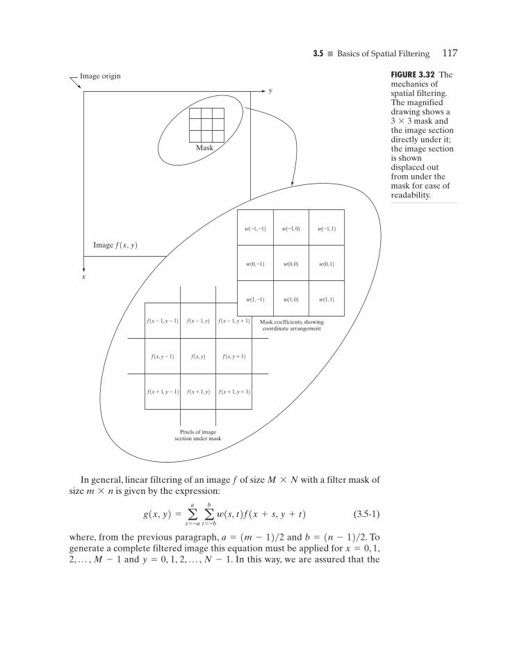
3.5 � Basics of Spatial Filtering 117
y
x
Image origin
Mask
Image f(x, y)
w(–1, –1)
f(x-1, y-1) f(x-1, y) f(x-1, y+1)
f(x, y-1) f(x, y) f(x, y+1)
f(x+1, y-1) f(x+1, y) f(x+1, y+1)
w(–1, 0) w(–1, 1)
w(0, –1) w(0, 0) w(0, 1)
w(1, –1) w(1, 0) w(1, 1)
Mask coefficients, showingcoordinate arrangement
Pixels of imagesection under mask
FIGURE 3.32 Themechanics ofspatial filtering.The magnifieddrawing shows a3*3 mask andthe image sectiondirectly under it;the image sectionis showndisplaced outfrom under themask for ease ofreadability.
In general, linear filtering of an image f of size M*N with a filter mask ofsize m*n is given by the expression:
(3.5-1)
where, from the previous paragraph, a=(m-1)�2 and b=(n-1)�2. Togenerate a complete filtered image this equation must be applied for x=0, 1,2, p , M-1 and y=0, 1, 2, p , N-1. In this way, we are assured that the
g(x, y) = aa
s = -a a
b
t = -bw(s, t)f(x + s, y + t)
GONZ03-075-146.II 29-08-2001 13:43 Page 117

118 Chapter 3 � Image Enhancement in the Spatial Domain
mask processes all pixels in the image. It is easily verified when m=n=3 thatthis expression reduces to the example given in the previous paragraph.
As discussed in Chapter 4, the process of linear filtering given in Eq. (3.5-1)is similar to a frequency domain concept called convolution. For this reason,linear spatial filtering often is referred to as “convolving a mask with an image.”Similarly, filter masks are sometimes called convolution masks. The term con-volution kernel also is in common use.
When interest lies on the response, R, of an m*n mask at any point (x, y),and not on the mechanics of implementing mask convolution, it is commonpractice to simplify the notation by using the following expression:
(3.5-2)
where the w’s are mask coefficients, the z’s are the values of the image graylevels corresponding to those coefficients, and mn is the total number of coef-ficients in the mask. For the 3*3 general mask shown in Fig. 3.33 the responseat any point (x, y) in the image is given by
(3.5-3)
We make special mention of this simple formula because it is seen frequentlyin the published literature on image processing.
Nonlinear spatial filters also operate on neighborhoods, and the mechanicsof sliding a mask past an image are the same as was just outlined. In general,however, the filtering operation is based conditionally on the values of the pix-els in the neighborhood under consideration, and they do not explicitly use co-efficients in the sum-of-products manner described in Eqs. (3.5-1) and (3.5-2).As shown in Section 3.6.2, for example, noise reduction can be achieved effec-tively with a nonlinear filter whose basic function is to compute the mediangray-level value in the neighborhood in which the filter is located. Computationof the median is a nonlinear operation, as is computation of the variance, whichwe used in Section 3.3.4.
= a9
i = 1wi zi .
R = w1 z1 + w2 z2 + p w9 z9
= amn
i = 1wi zi
R = w1 z1 + w2 z2 + p + wmn zmn
w1 w2 w3
w4 w5 w6
w7 w8 w9
FIGURE 3.33Anotherrepresentation ofa general 3*3spatial filter mask.
GONZ03-075-146.II 29-08-2001 13:43 Page 118
3.6 � Smoothing Spatial Filters 119
An important consideration in implementing neighborhood operations forspatial filtering is the issue of what happens when the center of the filter ap-proaches the border of the image. Consider for simplicity a square mask of sizen*n. At least one edge of such a mask will coincide with the border of theimage when the center of the mask is at a distance of (n-1)�2 pixels awayfrom the border of the image. If the center of the mask moves any closer to theborder, one or more rows or columns of the mask will be located outside theimage plane. There are several ways to handle this situation. The simplest is tolimit the excursions of the center of the mask to be at a distance no less than(n-1)�2 pixels from the border. The resulting filtered image will be smallerthan the original, but all the pixels in the filtered imaged will have beenprocessed with the full mask. If the result is required to be the same size as theoriginal, then the approach typically employed is to filter all pixels only with thesection of the mask that is fully contained in the image. With this approach,there will be bands of pixels near the border that will have been processed witha partial filter mask. Other approaches include “padding” the image by addingrows and columns of 0’s (or other constant gray level), or padding by replicat-ing rows or columns.The padding is then stripped off at the end of the process.This keeps the size of the filtered image the same as the original, but the valuesof the padding will have an effect near the edges that becomes more prevalentas the size of the mask increases.The only way to obtain a perfectly filtered re-sult is to accept a somewhat smaller filtered image by limiting the excursions ofthe center of the filter mask to a distance no less than (n-1)�2 pixels from theborder of the original image.
Smoothing Spatial Filters
Smoothing filters are used for blurring and for noise reduction. Blurring is usedin preprocessing steps, such as removal of small details from an image prior to(large) object extraction, and bridging of small gaps in lines or curves. Noisereduction can be accomplished by blurring with a linear filter and also by non-linear filtering.
3.6.1 Smoothing Linear FiltersThe output (response) of a smoothing, linear spatial filter is simply the averageof the pixels contained in the neighborhood of the filter mask. These filterssometimes are called averaging filters. For reasons explained in Chapter 4, theyalso are referred to a lowpass filters.
The idea behind smoothing filters is straightforward. By replacing the valueof every pixel in an image by the average of the gray levels in the neighbor-hood defined by the filter mask, this process results in an image with reduced“sharp” transitions in gray levels. Because random noise typically consists ofsharp transitions in gray levels, the most obvious application of smoothing isnoise reduction. However, edges (which almost always are desirable features ofan image) also are characterized by sharp transitions in gray levels, so averag-ing filters have the undesirable side effect that they blur edges. Another appli-cation of this type of process includes the smoothing of false contours that result
3.6
GONZ03-075-146.II 29-08-2001 13:43 Page 119

120 Chapter 3 � Image Enhancement in the Spatial Domain
1 1 1
119–* 1
16––*1 1
1 1 1
1 2 1
2 4 2
1 2 1
FIGURE 3.34 Two3*3 smoothing(averaging) filtermasks. Theconstant multiplier in front of eachmask is equal tothe sum of thevalues of itscoefficients, as isrequired tocompute anaverage.
from using an insufficient number of gray levels, as discussed in Section 2.4.3.A major use of averaging filters is in the reduction of “irrelevant” detail in animage. By “irrelevant” we mean pixel regions that are small with respect to thesize of the filter mask. This latter application is illustrated later in this section.
Figure 3.34 shows two 3*3 smoothing filters. Use of the first filter yields thestandard average of the pixels under the mask.This can best be seen by substi-tuting the coefficients of the mask into Eq. (3.5-3):
which is the average of the gray levels of the pixels in the 3*3 neighborhooddefined by the mask. Note that, instead of being 1�9, the coefficients of the fil-ter are all 1’s. The idea here is that it is computationally more efficient to havecoefficients valued 1. At the end of the filtering process the entire image is di-vided by 9.An m*n mask would have a normalizing constant equal to 1�mn.A spatial averaging filter in which all coefficients are equal is sometimes calleda box filter.
The second mask shown in Fig. 3.34 is a little more interesting. This maskyields a so-called weighted average, terminology used to indicate that pixels aremultiplied by different coefficients, thus giving more importance (weight) tosome pixels at the expense of others. In the mask shown in Fig. 3.34(b) the pixelat the center of the mask is multiplied by a higher value than any other, thus giv-ing this pixel more importance in the calculation of the average.The other pix-els are inversely weighted as a function of their distance from the center of themask. The diagonal terms are further away from the center than the orthogo-nal neighbors (by a factor of ) and, thus, are weighed less than these imme-diate neighbors of the center pixel.The basic strategy behind weighing the centerpoint the highest and then reducing the value of the coefficients as a functionof increasing distance from the origin is simply an attempt to reduce blurringin the smoothing process.We could have picked other weights to accomplish thesame general objective. However, the sum of all the coefficients in the mask ofFig. 3.34(b) is equal to 16, an attractive feature for computer implementation be-cause it has an integer power of 2. In practice, it is difficult in general to see dif-ferences between images smoothed by using either of the masks in Fig. 3.34, orsimilar arrangements, because the area these masks span at any one location inan image is so small.
12
R =19
a9
i = 1zi ,
a b
GONZ03-075-146.II 29-08-2001 13:43 Page 120

3.6 � Smoothing Spatial Filters 121
With reference to Eq. (3.5-1), the general implementation for filtering anM*N image with a weighted averaging filter of size m*n (m and n odd) isgiven by the expression
(3.6-1)
The parameters in this equation are as defined in Eq. (3.5-1). As before, it isunderstood that the complete filtered image is obtained by applying Eq. (3.6-1)for x=0, 1, 2, p , M-1 and y=0, 1, 2, p , N-1. The denominator inEq. (3.6-1) is simply the sum of the mask coefficients and, therefore, it is a con-stant that needs to be computed only once.Typically, this scale factor is appliedto all the pixels of the output image after the filtering process is completed.
� The effects of smoothing as a function of filter size are illustrated in Fig. 3.35,which shows an original image and the corresponding smoothed results obtainedusing square averaging filters of sizes n=3, 5, 9, 15, and 35 pixels, respectively.The principal features of these results are as follows: For n=3, we note a gen-eral slight blurring throughout the entire image but, as expected, details thatare of approximately the same size as the filter mask are affected considerablymore. For example, the 3*3 and 5*5 squares, the small letter “a,” and the finegrain noise show significant blurring when compared to the rest of the image.Apositive result is that the noise is less pronounced. Note that the jagged bordersof the characters and gray circles have been pleasingly smoothed.
The result for n=5 is somewhat similar, with a slight further increase inblurring. For n=9 we see considerably more blurring, and the 20% black cir-cle is not nearly as distinct from the background as in the previous three images,illustrating the blending effect that blurring has on objects whose gray levelcontent is close to that of its neighboring pixels. Note the significant furthersmoothing of the noisy rectangles. The results for n=15 and 35 are extremewith respect to the sizes of the objects in the image.This type of excessive blur-ring is generally used to eliminate small objects from an image. For instance, thethree small squares, two of the circles, and most of the noisy rectangle areashave been blended into the background of the image in Fig. 3.35(f). Note alsoin this figure the pronounced black border. This is a result of padding the bor-der of the original image with 0’s (black) and then trimming off the paddedarea. Some of the black was blended into all filtered images, but became trulyobjectionable for the images smoothed with the larger filters. �
As mentioned earlier, an important application of spatial averaging is to bluran image for the purpose getting a gross representation of objects of interest,such that the intensity of smaller objects blends with the background and larg-er objects become “bloblike” and easy to detect. The size of the mask estab-lishes the relative size of the objects that will be blended with the background.As an illustration, consider Fig. 3.36(a), which is an image from the Hubble tele-scope in orbit around the Earth. Figure 3.36(b) shows the result of applying a
g(x, y) =a
a
s = -a a
b
t = -bw(s, t)f(x + s, y + t)
aa
s = -a a
b
t = -bw(s, t)
EXAMPLE 3.9:Image smoothingwith masks ofvarious sizes.
GONZ03-075-146.II 29-08-2001 13:43 Page 121

122 Chapter 3 � Image Enhancement in the Spatial Domain
FIGURE 3.35 (a) Original image, of size 500*500 pixels. (b)–(f) Results of smoothingwith square averaging filter masks of sizes n=3, 5, 9, 15, and 35, respectively.The blacksquares at the top are of sizes 3, 5, 9, 15, 25, 35, 45, and 55 pixels, respectively; their bor-ders are 25 pixels apart. The letters at the bottom range in size from 10 to 24 points, inincrements of 2 points; the large letter at the top is 60 points.The vertical bars are 5 pix-els wide and 100 pixels high; their separation is 20 pixels. The diameter of the circles is25 pixels, and their borders are 15 pixels apart; their gray levels range from 0% to 100%black in increments of 20%. The background of the image is 10% black. The noisy rec-tangles are of size 50*120 pixels.
a bce
df
GONZ03-075-146.II 29-08-2001 13:43 Page 122

3.6 � Smoothing Spatial Filters 123
FIGURE 3.36 (a) Image from the Hubble Space Telescope. (b) Image processed by a 15*15 averaging mask.(c) Result of thresholding (b). (Original image courtesy of NASA.)
15*15 averaging mask to this image.We see that a number of objects have ei-ther blended with the background or their intensity has diminished considerably.It is typical to follow an operation like this with thresholding to eliminate ob-jects based on their intensity. The result of using the thresholding function ofFig. 3.2(b) with a threshold value equal to 25% of the highest intensity in theblurred image is shown in Fig. 3.36(c). Comparing this result with the originalimage, we see that it is a reasonable representation of what we would considerto be the largest, brightest objects in that image.
3.6.2 Order-Statistics FiltersOrder-statistics filters are nonlinear spatial filters whose response is based onordering (ranking) the pixels contained in the image area encompassed bythe filter, and then replacing the value of the center pixel with the value de-termined by the ranking result.The best-known example in this category is themedian filter, which, as its name implies, replaces the value of a pixel by themedian of the gray levels in the neighborhood of that pixel (the original valueof the pixel is included in the computation of the median). Median filters arequite popular because, for certain types of random noise, they provide excel-lent noise-reduction capabilities, with considerably less blurring than linearsmoothing filters of similar size. Median filters are particularly effective inthe presence of impulse noise, also called salt-and-pepper noise because of itsappearance as white and black dots superimposed on an image.
The median, j, of a set of values is such that half the values in the set are lessthan or equal to j, and half are greater than or equal to j. In order to performmedian filtering at a point in an image, we first sort the values of the pixel inquestion and its neighbors, determine their median, and assign this value to thatpixel. For example, in a 3*3 neighborhood the median is the 5th largest value,in a 5*5 neighborhood the 13th largest value, and so on.When several values
a b c
GONZ03-075-146.II 29-08-2001 13:43 Page 123
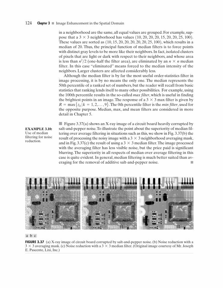
124 Chapter 3 � Image Enhancement in the Spatial Domain
in a neighborhood are the same, all equal values are grouped. For example, sup-pose that a 3*3 neighborhood has values (10, 20, 20, 20, 15, 20, 20, 25, 100).These values are sorted as (10, 15, 20, 20, 20, 20, 20, 25, 100), which results in amedian of 20. Thus, the principal function of median filters is to force pointswith distinct gray levels to be more like their neighbors. In fact, isolated clustersof pixels that are light or dark with respect to their neighbors, and whose areais less than n2�2 (one-half the filter area), are eliminated by an n*n medianfilter. In this case “eliminated” means forced to the median intensity of theneighbors. Larger clusters are affected considerably less.
Although the median filter is by far the most useful order-statistics filter inimage processing, it is by no means the only one. The median represents the50th percentile of a ranked set of numbers, but the reader will recall from basicstatistics that ranking lends itself to many other possibilities. For example, usingthe 100th percentile results in the so-called max filter, which is useful in findingthe brightest points in an image. The response of a 3*3 max filter is given byR=max Ezk |k=1, 2, p , 9F .The 0th percentile filter is the min filter, used forthe opposite purpose. Median, max, and mean filters are considered in moredetail in Chapter 5.
� Figure 3.37(a) shows an X-ray image of a circuit board heavily corrupted bysalt-and-pepper noise.To illustrate the point about the superiority of median fil-tering over average filtering in situations such as this, we show in Fig. 3.37(b) theresult of processing the noisy image with a 3*3 neighborhood averaging mask,and in Fig. 3.37(c) the result of using a 3*3 median filter.The image processedwith the averaging filter has less visible noise, but the price paid is significantblurring. The superiority in all respects of median over average filtering in thiscase is quite evident. In general, median filtering is much better suited than av-eraging for the removal of additive salt-and-pepper noise. �
EXAMPLE 3.10:Use of medianfiltering for noisereduction.
FIGURE 3.37 (a) X-ray image of circuit board corrupted by salt-and-pepper noise. (b) Noise reduction with a3*3 averaging mask. (c) Noise reduction with a 3*3 median filter. (Original image courtesy of Mr. JosephE. Pascente, Lixi, Inc.)
a b c
GONZ03-075-146.II 29-08-2001 13:43 Page 124

3.7 � Sharpening Spatial Filters 125
Sharpening Spatial Filters
The principal objective of sharpening is to highlight fine detail in an image orto enhance detail that has been blurred, either in error or as a natural effect ofa particular method of image acquisition. Uses of image sharpening vary and in-clude applications ranging from electronic printing and medical imaging to in-dustrial inspection and autonomous guidance in military systems.
In the last section, we saw that image blurring could be accomplished in thespatial domain by pixel averaging in a neighborhood. Since averaging is analo-gous to integration, it is logical to conclude that sharpening could be accom-plished by spatial differentiation. This, in fact, is the case, and the discussion inthis section deals with various ways of defining and implementing operators forsharpening by digital differentiation. Fundamentally, the strength of the re-sponse of a derivative operator is proportional to the degree of discontinuity ofthe image at the point at which the operator is applied. Thus, image differenti-ation enhances edges and other discontinuities (such as noise) and deempha-sizes areas with slowly varying gray-level values.
3.7.1 FoundationIn the two sections that follow, we consider in some detail sharpening filters thatare based on first- and second-order derivatives, respectively. Before proceedingwith that discussion, however, we stop to look at some of the fundamental prop-erties of these derivatives in a digital context. To simplify the explanation, wefocus attention on one-dimensional derivatives. In particular, we are interestedin the behavior of these derivatives in areas of constant gray level (flat segments),at the onset and end of discontinuities (step and ramp discontinuities), and alonggray-level ramps.These types of discontinuities can be used to model noise points,lines, and edges in an image. The behavior of derivatives during transitions intoand out of these image features also is of interest.
The derivatives of a digital function are defined in terms of differences.Thereare various ways to define these differences. However, we require that any de-finition we use for a first derivative (1) must be zero in flat segments (areas ofconstant gray-level values); (2) must be nonzero at the onset of a gray-levelstep or ramp; and (3) must be nonzero along ramps. Similarly, any definition ofa second derivative (1) must be zero in flat areas; (2) must be nonzero at theonset and end of a gray-level step or ramp; and (3) must be zero along rampsof constant slope. Since we are dealing with digital quantities whose values arefinite, the maximum possible gray-level change also is finite, and the shortest dis-tance over which that change can occur is between adjacent pixels.
A basic definition of the first-order derivative of a one-dimensional func-tion f(x) is the difference
We used a partial derivative here in order to keep the notation the same aswhen we consider an image function of two variables, f(x, y), at which time we
0f
0x= f(x + 1) - f(x).
3.7
GONZ03-075-146.II 29-08-2001 13:43 Page 125

126 Chapter 3 � Image Enhancement in the Spatial Domain
Second Derivative
First Derivative
Image strip
Gra
y le
vel p
rofi
le
5
76543210
5 4 3 2 1 0 0 0 6 0 0 0 0 1 3 1 0 0 0 0 7 7 7
–1 –1 –1 –1 –1 0 0 6 –6 0 0 0 1 2 –2 –1 0 0 0 7 0 0 0
–1 0 0 0 0 1 0 6 –12 6 0 0 1 1 –4 1 1 0 0 7 –7 0 0
7
Ramp
Isolated point
Thin line
Flat segment
Step
FIGURE 3.38(a) A simpleimage. (b) 1-Dhorizontal gray-level profile alongthe center of theimage andincluding theisolated noisepoint.(c) Simplifiedprofile (the pointsare joined bydashed lines tosimplifyinterpretation).
will be dealing with partial derivatives along the two spatial axes. Use of a par-tial derivative in the present discussion does not affect in any way the nature ofwhat we are trying to accomplish.
Similarly, we define a second-order derivative as the difference
It is easily verified that these two definitions satisfy the conditions stated pre-viously regarding derivatives of the first and second order.To see this, and alsoto highlight the fundamental similarities and differences between first- and sec-ond-order derivatives in the context of image processing, consider the exampleshown in Fig. 3.38.
Figure 3.38(a) shows a simple image that contains various solid objects, aline, and a single noise point. Figure 3.38(b) shows a horizontal gray-level pro-file (scan line) of the image along the center and including the noise point.Thisprofile is the one-dimensional function we will use for illustrations regarding thisfigure. Figure 3.38(c) shows a simplification of the profile, with just enough num-
02f
0x2 = f(x + 1) + f(x - 1) - 2f(x).
a bc
GONZ03-075-146.II 29-08-2001 13:43 Page 126

3.7 � Sharpening Spatial Filters 127
bers to make it possible for us to analyze how the first- and second-order de-rivatives behave as they encounter a noise point, a line, and then the edge of anobject. In our simplified diagram the transition in the ramp spans four pixels, thenoise point is a single pixel, the line is three pixels thick, and the transition intothe gray-level step takes place between adjacent pixels.The number of gray lev-els was simplified to only eight levels.
Let us consider the properties of the first and second derivatives as we tra-verse the profile from left to right. First, we note that the first-order derivativeis nonzero along the entire ramp, while the second-order derivative is nonzeroonly at the onset and end of the ramp. Because edges in an image resemble thistype of transition, we conclude that first-order derivatives produce “thick” edgesand second-order derivatives, much finer ones. Next we encounter the isolatednoise point. Here, the response at and around the point is much stronger forthe second- than for the first-order derivative. Of course, this is not unexpect-ed. A second-order derivative is much more aggressive than a first-order de-rivative in enhancing sharp changes. Thus, we can expect a second-orderderivative to enhance fine detail (including noise) much more than a first-orderderivative. The thin line is a fine detail, and we see essentially the same differ-ence between the two derivatives. If the maximum gray level of the line hadbeen the same as the isolated point, the response of the second derivative wouldhave been stronger for the latter. Finally, in this case, the response of the two de-rivatives is the same at the gray-level step (in most cases when the transition intoa step is not from zero, the second derivative will be weaker).We also note thatthe second derivative has a transition from positive back to negative. In animage, this shows as a thin double line.This “double-edge” effect is an issue thatwill be important in Chapter 10, where we use derivatives for edge detection.It is of interest also to note that if the gray level of the thin line had been thesame as the step, the response of the second derivative would have been strongerfor the line than for the step.
In summary, comparing the response between first- and second-order de-rivatives, we arrive at the following conclusions. (1) First-order derivatives gen-erally produce thicker edges in an image. (2) Second-order derivatives have astronger response to fine detail, such as thin lines and isolated points. (3) First-order derivatives generally have a stronger response to a gray-level step. (4) Sec-ond-order derivatives produce a double response at step changes in gray level.We also note of second-order derivatives that, for similar changes in gray-levelvalues in an image, their response is stronger to a line than to a step, and to apoint than to a line.
In most applications, the second derivative is better suited than the first de-rivative for image enhancement because of the ability of the former to enhancefine detail. For this, and for reasons of simpler implementation and extensions,we will focus attention initially on uses of the second derivative for enhance-ment. First-order derivatives are discussed in Section 3.7.3. Although the prin-ciple of use of first derivatives in image processing is for edge extraction, theydo have important uses in image enhancement. In fact, we show in Section 3.8that they can be used in conjunction with the second derivative to obtain someimpressive enhancement results.
GONZ03-075-146.II 29-08-2001 13:43 Page 127
128 Chapter 3 � Image Enhancement in the Spatial Domain
3.7.2 Use of Second Derivatives for Enhancement–The LaplacianIn this section we consider in some detail the use of two-dimensional, second-order derivatives for image enhancement.The approach basically consists of defin-ing a discrete formulation of the second-order derivative and then constructinga filter mask based on that formulation. We are interested in isotropic filters,whose response is independent of the direction of the discontinuities in the imageto which the filter is applied. In other words, isotropic filters are rotation invari-ant, in the sense that rotating the image and then applying the filter gives thesame result as applying the filter to the image first and then rotating the result.
Development of the method
It can be shown (Rosenfeld and Kak [1982]) that the simplest isotropic deriv-ative operator is the Laplacian, which, for a function (image) f(x, y) of twovariables, is defined as
(3.7-1)
Because derivatives of any order are linear operations, the Laplacian is a lin-ear operator.
In order to be useful for digital image processing, this equation needs to beexpressed in discrete form.There are several ways to define a digital Laplacianusing neighborhoods. Whatever the definition, however, it has to satisfy theproperties of a second derivative outlined in Section 3.7.1.The definition of thedigital second derivative given in that section is one of the most used.Taking intoaccount that we now have two variables, we use the following notation for thepartial second-order derivative in the x-direction:
(3.7-2)
and, similarly in the y-direction, as
(3.7-3)
The digital implementation of the two-dimensional Laplacian in Eq. (3.7-1) isobtained by summing these two components:
(3.7-4)
This equation can be implemented using the mask shown in Fig. 3.39(a), whichgives an isotropic result for rotations in increments of 90°. The mechanics ofimplementation are given in Eq. (3.5-1) and are illustrated in Section 3.6.1 forthe linear smoothing filters. We simply are using different coefficients here.
The diagonal directions can be incorporated in the definition of the digitalLaplacian by adding two more terms to Eq. (3.7-4), one for each of the twodiagonal directions.The form of each new term is the same as either Eq. (3.7-2)
- 4f(x, y).
§ 2f = Cf(x + 1, y) + f(x - 1, y) + f(x, y + 1) + f(x, y - 1) D
02f
02y2 = f(x, y + 1) + f(x, y - 1) - 2f(x, y)
02f
02x2 = f(x + 1, y) + f(x - 1, y) - 2f(x, y)
§ 2f =02f
0x2 +02f
0y2 .
GONZ03-075-146.II 29-08-2001 13:43 Page 128
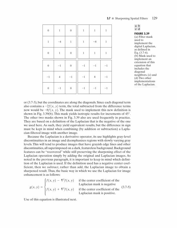
3.7 � Sharpening Spatial Filters 129
0 1 0
1 –4 1
0 1 0
1 1 1
1 –8 1
1 1 1
0 –1 0
–1 4 –1
0 –1 0
–1 –1 –1
–1 8 –1
–1 –1 –1
FIGURE 3.39(a) Filter maskused toimplement thedigital Laplacian,as defined inEq. (3.7-4).(b) Mask used toimplement anextension of thisequation thatincludes thediagonalneighbors. (c) and(d) Two otherimplementationsof the Laplacian.
or (3.7-3), but the coordinates are along the diagonals. Since each diagonal termalso contains a –2f(x, y) term, the total subtracted from the difference termsnow would be –8f(x, y). The mask used to implement this new definition isshown in Fig. 3.39(b). This mask yields isotropic results for increments of 45°.The other two masks shown in Fig. 3.39 also are used frequently in practice.They are based on a definition of the Laplacian that is the negative of the onewe used here. As such, they yield equivalent results, but the difference in signmust be kept in mind when combining (by addition or subtraction) a Lapla-cian-filtered image with another image.
Because the Laplacian is a derivative operator, its use highlights gray-leveldiscontinuities in an image and deemphasizes regions with slowly varying graylevels. This will tend to produce images that have grayish edge lines and otherdiscontinuities, all superimposed on a dark, featureless background. Backgroundfeatures can be “recovered” while still preserving the sharpening effect of theLaplacian operation simply by adding the original and Laplacian images. Asnoted in the previous paragraph, it is important to keep in mind which defini-tion of the Laplacian is used. If the definition used has a negative center coef-ficient, then we subtract, rather than add, the Laplacian image to obtain asharpened result. Thus, the basic way in which we use the Laplacian for imageenhancement is as follows:
(3.7-5)
Use of this equation is illustrated next.
g(x, y) = df(x, y) - § 2f(x, y)
f(x, y) + § 2f(x, y)
if the center coefficient of theLaplacian mask is negative
if the center coefficient of theLaplacian mask is positive.
a bc d
GONZ03-075-146.II 29-08-2001 13:43 Page 129

130 Chapter 3 � Image Enhancement in the Spatial Domain
FIGURE 3.40(a) Image of theNorth Pole of themoon.(b) Laplacian-filtered image.(c) Laplacianimage scaled fordisplay purposes.(d) Imageenhanced byusing Eq. (3.7-5).(Original imagecourtesy ofNASA.)
� Figure 3.40(a) shows an image of the North Pole of the moon. Figure 3.40(b)shows the result of filtering this image with the Laplacian mask in Fig. 3.39(b).Since the Laplacian image contains both positive and negative values, a typicalway to scale it is to use the approach discussed at the end of Section 3.4.1. Some-times one encounters the absolute value being used for this purpose, but this re-ally is not correct because it produces double lines of nearly equal magnitude,which can be confusing.
The image shown in Fig. 3.40(c) was scaled in the manner just described fordisplay purposes. Note that the dominant features of the image are edges andsharp gray-level discontinuities of various gray-level values. The background,previously near black, is now gray due to the scaling. This grayish appearanceis typical of Laplacian images that have been scaled properly. Finally, Fig. 3.40(d)
EXAMPLE 3.11:Imagingsharpening withthe Laplacian.
a bc d
GONZ03-075-146.II 29-08-2001 13:43 Page 130
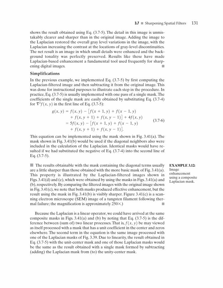
3.7 � Sharpening Spatial Filters 131
shows the result obtained using Eq. (3.7-5). The detail in this image is unmis-takably clearer and sharper than in the original image. Adding the image tothe Laplacian restored the overall gray level variations in the image, with theLaplacian increasing the contrast at the locations of gray-level discontinuities.The net result is an image in which small details were enhanced and the back-ground tonality was perfectly preserved. Results like these have madeLaplacian-based enhancement a fundamental tool used frequently for sharp-ening digital images. �
Simplifications
In the previous example, we implemented Eq. (3.7-5) by first computing theLaplacian-filtered image and then subtracting it from the original image. Thiswas done for instructional purposes to illustrate each step in the procedure. Inpractice, Eq. (3.7-5) is usually implemented with one pass of a single mask.Thecoefficients of the single mask are easily obtained by substituting Eq. (3.7-4)for in the first line of Eq. (3.7-5):
(3.7-6)
This equation can be implemented using the mask shown in Fig. 3.41(a). Themask shown in Fig. 3.41(b) would be used if the diagonal neighbors also wereincluded in the calculation of the Laplacian. Identical masks would have re-sulted if we had substituted the negative of Eq. (3.7-4) into the second line ofEq. (3.7-5).
� The results obtainable with the mask containing the diagonal terms usuallyare a little sharper than those obtained with the more basic mask of Fig. 3.41(a).This property is illustrated by the Laplacian-filtered images shown inFigs. 3.41(d) and (e), which were obtained by using the masks in Figs. 3.41(a) and(b), respectively. By comparing the filtered images with the original image shownin Fig. 3.41(c), we note that both masks produced effective enhancement, but theresult using the mask in Fig. 3.41(b) is visibly sharper. Figure 3.41(c) is a scan-ning electron microscope (SEM) image of a tungsten filament following ther-mal failure; the magnification is approximately 250 *.) �
Because the Laplacian is a linear operator, we could have arrived at the samecomposite masks in Figs. 3.41(a) and (b) by noting that Eq. (3.7-5) is the dif-ference between (sum of) two linear processes. That is, f(x, y) be may viewedas itself processed with a mask that has a unit coefficient in the center and zeroselsewhere. The second term in the equation is the same image processed withone of the Laplacian masks of Fig. 3.39. Due to linearity, the result obtained inEq. (3.7-5) with the unit-center mask and one of those Laplacian masks wouldbe the same as the result obtained with a single mask formed by subtracting(adding) the Laplacian mask from (to) the unity-center mask.
+ f(x, y + 1) + f(x, y - 1) D . = 5f(x, y) - Cf(x + 1, y) + f(x - 1, y)
+ f(x, y + 1) + f(x, y - 1) D + 4f(x, y)
g(x, y) = f(x, y) - Cf(x + 1, y) + f(x - 1, y)
§ 2f(x, y)
EXAMPLE 3.12:Imageenhancementusing a compositeLaplacian mask.
GONZ03-075-146.II 29-08-2001 13:43 Page 131

132 Chapter 3 � Image Enhancement in the Spatial Domain
0 –1 0
–1 5 –1
0 –1 0–1 –1 –1
–1 9 –1
–1 –1 –1
FIGURE 3.41 (a) Composite Laplacian mask. (b) A second composite mask. (c) Scanningelectron microscope image. (d) and (e) Results of filtering with the masks in (a) and (b),respectively.Note how much sharper (e) is than (d). (Original image courtesy of Mr.MichaelShaffer, Department of Geological Sciences, University of Oregon, Eugene.)
Unsharp masking and high-boost filtering
A process used for many years in the publishing industry to sharpen imagesconsists of subtracting a blurred version of an image from the image itself.Thisprocess, called unsharp masking, is expressed as
(3.7-7)
where fs(x, y) denotes the sharpened image obtained by unsharp masking, andis a blurred version of f(x, y).The origin of unsharp masking is in dark-
room photography, where it consists of clamping together a blurred negative toa corresponding positive film and then developing this combination to producea sharper image.
A slight further generalization of unsharp masking is called high-boostfiltering. A high-boost filtered image, fhb, is defined at any point (x, y) as
(3.7-8)fhb(x, y) = Af(x, y) - f–
(x, y)
f–
(x, y)
fs(x, y) = f(x, y) - f–
(x, y)
a b cd e
GONZ03-075-146.II 29-08-2001 13:43 Page 132

3.7 � Sharpening Spatial Filters 133
0 –1 0
–1 A+4 –1
0 –1 0
–1 –1 –1
–1 A+8 –1
–1 –1 –1
FIGURE 3.42 Thehigh-boost filteringtechnique can beimplemented witheither one of thesemasks, with A � 1.
where A � 1 and, as before, is a blurred version of f. This equation maybe written as
(3.7-9)
By using Eq. (3.7-7), we obtain
(3.7-10)
as the expression for computing a high-boost-filtered image.Equation (3.7-10) is applicable in general and does not state explicitly how
the sharp image is obtained. If we elect to use the Laplacian, then we know thatfs(x, y) can be obtained using Eq. (3.7-5). In this case, Eq. (3.7-10) becomes
(3.7-11)
High-boost filtering can be implemented with one pass using either of the twomasks shown in Fig. 3.42. Note that, when A=1, high-boost filtering becomes“standard” Laplacian sharpening. As the value of A increases past 1, the con-tribution of the sharpening process becomes less and less important. Eventual-ly, if A is large enough, the high-boost image will be approximately equal to theoriginal image multiplied by a constant.
� One of the principal applications of boost filtering is when the input image isdarker than desired. By varying the boost coefficient, it generally is possible toobtain an overall increase in average gray level of the image, thus helping to bright-en the final result. Figure 3.43 shows such an application. Part (a) of this figure isa darker version of the image in Fig. 3.41(c). Figure 3.43(b) shows the Laplaciancomputed using the mask in Fig. 3.42(b), with A=0. Figure 3.43(c) was obtainedusing the mask in Fig. 3.42(b) with A=1. As expected, the image has beensharpened, but it is still as dark as the original. Finally, Fig. 3.43(d) shows the re-sult of using A=1.7.This is a much more acceptable result, in which the averagegray level has increased, thus making the image lighter and more natural. �
fhb = dAf(x, y) - § 2f(x, y)
Af(x, y) + § 2f(x, y)
if the center coefficient of theLaplacian mask is negative
if the center coefficient of theLaplacian mask is positive.
fhb(x, y) = (A - 1)f(x, y) + fs(x, y)
fhb(x, y) = (A - 1)f(x, y) + f(x, y) - f–
(x, y).
f–
EXAMPLE 3.13:Imageenhancement witha high-boost filter.
a b
GONZ03-075-146.II 29-08-2001 13:43 Page 133

134 Chapter 3 � Image Enhancement in the Spatial Domain
FIGURE 3.43(a) Same asFig. 3.41(c), butdarker.(a) Laplacian of(a) computed withthe mask inFig. 3.42(b) usingA=0.(c) Laplacianenhanced imageusing the mask inFig. 3.42(b) withA=1. (d) Sameas (c), but usingA=1.7.
3.7.3 Use of First Derivatives for Enhancement—The GradientFirst derivatives in image processing are implemented using the magnitude ofthe gradient. For a function f(x, y), the gradient of f at coordinates (x, y) is de-fined as the two-dimensional column vector
(3.7-12)
The magnitude of this vector is given by
(3.7-13)
The components of the gradient vector itself are linear operators, but the mag-nitude of this vector obviously is not because of the squaring and square root
= B a 0f
0xb 2
+ a 0f
0yb 2R 1�2
.
= CG2x + G2
y D 1�2 §f = mag (§f)
§f = BGx
GyR = D 0f
0x0f
0y
T .
a bc d
GONZ03-075-146.II 29-08-2001 13:43 Page 134

3.7 � Sharpening Spatial Filters 135
operations. On the other hand, the partial derivatives in Eq. (3.7-12) are not ro-tation invariant (isotropic), but the magnitude of the gradient vector is. Al-though it is not strictly correct, the magnitude of the gradient vector often isreferred to as the gradient. In keeping with tradition, we will use this term in thefollowing discussions, explicitly referring to the vector or its magnitude only incases where confusion is likely.
The computational burden of implementing Eq. (3.7-13) over an entire imageis not trivial, and it is common practice to approximate the magnitude of the gra-dient by using absolute values instead of squares and square roots:
(3.7-14)
This equation is simpler to compute and it still preserves relative changes ingray levels, but the isotropic feature property is lost in general. However, as inthe case of the Laplacian, the isotropic properties of the digital gradient de-fined in the following paragraph are preserved only for a limited number of ro-tational increments that depend on the masks used to approximate thederivatives. As it turns out, the most popular masks used to approximate thegradient give the same result only for vertical and horizontal edges and thusthe isotropic properties of the gradient are preserved only for multiples of 90°.These results are independent of whether Eq. (3.7-13) or (3.7-14) is used, sonothing of significance is lost in using the simpler of the two equations.
As in the case of the Laplacian, we now define digital approximations to thepreceding equations, and from there formulate the appropriate filter masks. Inorder to simplify the discussion that follows, we will use the notation inFig. 3.44(a) to denote image points in a 3*3 region. For example, the centerpoint, z5 , denotes f(x, y), z1 denotes f(x-1, y-1), and so on. As indicatedin Section 3.7.1, the simplest approximations to a first-order derivative that sat-isfy the conditions stated in that section are Gx=Az8-z5B and Gy=Az6-z5B .Two other definitions proposed by Roberts [1965] in the early development ofdigital image processing use cross differences:
(3.7-15)
If we elect to use Eq. (3.7-13), then we compute the gradient as
(3.7-16)
If we use absolute values, then substituting the quantities in Eq. (3.7-15) intoEq. (3.7-14) gives us the following approximation to the gradient:
(3.7-17)
This equation can be implemented with the two masks shown in Figs. 3.44(b) and(c). These masks are referred to as the Roberts cross-gradient operators.
Masks of even size are awkward to implement. The smallest filter mask inwhich we are interested is of size 3*3. An approximation using absolute val-ues, still at point z5 , but using a 3*3 mask, is
(3.7-18) + @ Az3 + 2z6 + z9B - Az1 + 2z4 + z7B @ . §f L @ Az7 + 2z8 + z9B - Az1 + 2z2 + z3B @
§f L @z9 - z5 @ + @z8 - z6 @ .
§f = C Az9 - z5B2 + Az8 - z6B2 D 1�2
Gx = Az9 - z5B and Gy = Az8 - z6B.
§f L @Gx @ + @Gy @ .
GONZ03-075-146.II 29-08-2001 13:43 Page 135
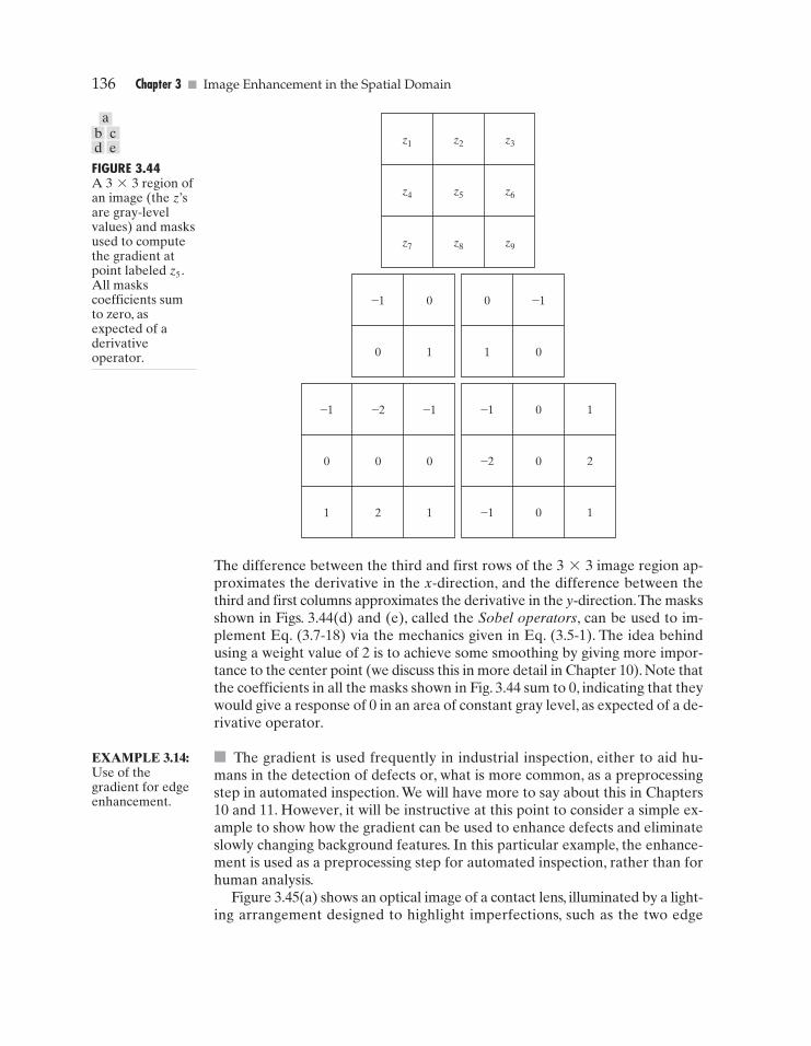
136 Chapter 3 � Image Enhancement in the Spatial Domain
–1 0
0 1
0 –1
1 0
–1 –2 –1
0 0 0
1 2 1
–1 0 1
–2 0 2
–1 0 1
z1 z2 z3
z4 z5 z6
z7 z8 z9
FIGURE 3.44A 3*3 region ofan image (the z’sare gray-levelvalues) and masksused to computethe gradient atpoint labeled z5 .All maskscoefficients sumto zero, asexpected of aderivativeoperator.
The difference between the third and first rows of the 3*3 image region ap-proximates the derivative in the x-direction, and the difference between thethird and first columns approximates the derivative in the y-direction.The masksshown in Figs. 3.44(d) and (e), called the Sobel operators, can be used to im-plement Eq. (3.7-18) via the mechanics given in Eq. (3.5-1). The idea behindusing a weight value of 2 is to achieve some smoothing by giving more impor-tance to the center point (we discuss this in more detail in Chapter 10). Note thatthe coefficients in all the masks shown in Fig. 3.44 sum to 0, indicating that theywould give a response of 0 in an area of constant gray level, as expected of a de-rivative operator.
� The gradient is used frequently in industrial inspection, either to aid hu-mans in the detection of defects or, what is more common, as a preprocessingstep in automated inspection. We will have more to say about this in Chapters10 and 11. However, it will be instructive at this point to consider a simple ex-ample to show how the gradient can be used to enhance defects and eliminateslowly changing background features. In this particular example, the enhance-ment is used as a preprocessing step for automated inspection, rather than forhuman analysis.
Figure 3.45(a) shows an optical image of a contact lens, illuminated by a light-ing arrangement designed to highlight imperfections, such as the two edge
EXAMPLE 3.14:Use of thegradient for edgeenhancement.
b cd e
a
GONZ03-075-146.II 29-08-2001 13:43 Page 136

3.8 � Combining Spatial Enhancement Methods 137
FIGURE 3.45Optical image ofcontact lens (notedefects on theboundary at 4 and5 o’clock).(b) Sobelgradient.(Original imagecourtesy ofMr. Pete Sites,PercepticsCorporation.)
a b
defects in the lens boundary seen at 4 and 5 o’clock. Figure 3.45(b) shows thegradient obtained using Eq. (3.7-14) with the two Sobel masks in Figs. 3.44(d)and (e).The edge defects also are quite visible in this image, but with the addedadvantage that constant or slowly varying shades of gray have been eliminat-ed, thus simplifying considerably the computational task required for auto-mated inspection. Note also that the gradient process highlighted small specsthat are not readily visible in the gray-scale image (specs like these can be for-eign matter, air pockets in a supporting solution, or miniscule imperfections inthe lens). The ability to enhance small discontinuities in an otherwise flat grayfield is another important feature of the gradient. �
Combining Spatial Enhancement Methods
With a few exceptions, like combining blurring with thresholding in Section 3.6.1,we have focused attention thus far on individual enhancement approaches. Fre-quently, a given enhancement task will require application of several comple-mentary enhancement techniques in order to achieve an acceptable result. Inthis section we illustrate by means of an example how to combine several of theapproaches developed in this chapter to address a difficult enhancement task.
The image shown in Fig. 3.46(a) is a nuclear whole body bone scan, used todetect diseases such as bone infection and tumors. Our objective is to enhancethis image by sharpening it and by bringing out more of the skeletal detail.Thenarrow dynamic range of the gray levels and high noise content make this imagedifficult to enhance. The strategy we will follow is to utilize the Laplacian tohighlight fine detail, and the gradient to enhance prominent edges. For reasonsthat will be explained shortly, a smoothed version of the gradient image will beused to mask the Laplacian image (see Section 3.4 regarding masking). Final-ly, we will attempt to increase the dynamic range of the gray levels by using agray-level transformation.
Figure 3.46 (b) shows the Laplacian of the original image, obtained usingthe mask in Fig. 3.39(d). This image was scaled (for display only) using thesame technique as in Fig. 3.40. We can obtain a sharpened image at this point
3.8
GONZ03-075-146.II 29-08-2001 13:43 Page 137

138 Chapter 3 � Image Enhancement in the Spatial Domain
FIGURE 3.46(a) Image ofwhole body bonescan.(b) Laplacian of(a). (c) Sharpenedimage obtainedby adding (a) and(b). (d) Sobel of(a).
a bc d
GONZ03-075-146.II 29-08-2001 13:43 Page 138
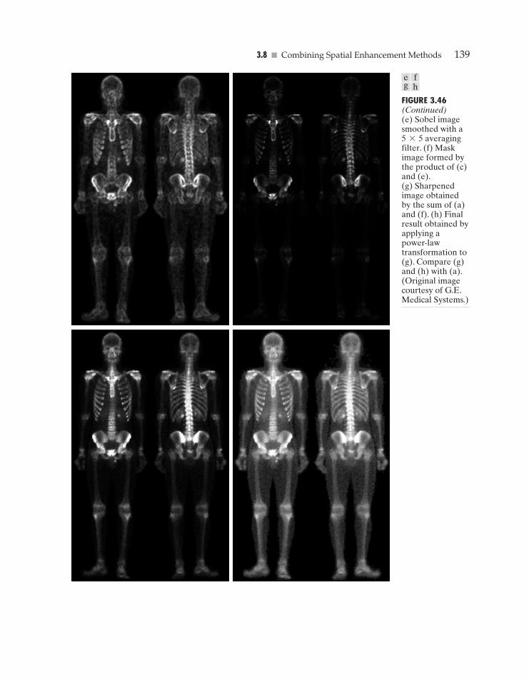
3.8 � Combining Spatial Enhancement Methods 139
FIGURE 3.46(Continued)(e) Sobel imagesmoothed with a5*5 averagingfilter. (f) Maskimage formed bythe product of (c)and (e).(g) Sharpenedimage obtainedby the sum of (a)and (f). (h) Finalresult obtained byapplying a power-lawtransformation to(g). Compare (g)and (h) with (a).(Original imagecourtesy of G.E.Medical Systems.)
e fg h
GONZ03-075-146.II 29-08-2001 13:43 Page 139

140 Chapter 3 � Image Enhancement in the Spatial Domain
simply by adding Figs. 3.46(a) and (b), which are an implementation of thesecond line in Eq. (3.7-5) (we used a mask with a positive center coefficient).Just by looking at the noise level in (b), we would expect a rather noisy sharp-ened image if we added Figs. 3.46(a) and (b), a fact that is confirmed by theresult shown in Fig. 3.46(c). One way that comes immediately to mind to re-duce the noise is to use a median filter. However, median filtering is a non-linear process capable of removing image features. This is unacceptable inmedical image processing.
An alternate approach is to use a mask formed from a smoothed version ofthe gradient of the original image. The motivation behind this is straightfor-ward and is based on the properties of first- and second-order derivatives ex-plained in Section 3.7.1.The Laplacian, being a second-order derivative operator,has the definite advantage that it is superior in enhancing fine detail. Howev-er, this causes it to produce noisier results than the gradient. This noise is mostobjectionable in smooth areas, where it tends to be more visible. The gradienthas a stronger response in areas of significant gray-level transitions (gray-levelramps and steps) than does the Laplacian.The response of the gradient to noiseand fine detail is lower than the Laplacian’s and can be lowered further bysmoothing the gradient with an averaging filter.The idea, then, is to smooth thegradient and multiply it by the Laplacian image. In this context, we may viewthe smoothed gradient as a mask image. The product will preserve details inthe strong areas while reducing noise in the relatively flat areas.This process canbe viewed roughly as combining the best features of the Laplacian and the gra-dient.The result is added to the original to obtain a final sharpened image, andcould even be used in boost filtering.
Figure 3.46(d) shows the Sobel gradient of the original image, computedusing Eq. (3.7-14). Components Gx and Gy were obtained using the masks inFigs. 3.44(d) and (e), respectively. As expected from our discussion in Section3.7.1, edges are much more dominant in this image than in the Laplacian image.The smoothed gradient image shown in Fig. 3.46(e) was obtained by using anaveraging filter of size 5*5. The two gradient images were scaled for displayin the same manner as the two Laplacian images. Because the smallest possiblevalue of a gradient image is 0, the background is black in the scaled gradient im-ages, rather than gray as in the scaled Laplacian.The fact that Figs. 3.46(d) and(e) are much brighter than Fig. 3.46(b) is again evidence that the gradient of animage with significant edge content has values that are higher in general thanin a Laplacian image.
The product of the Laplacian and smoothed-gradient image is shown inFig. 3.46(f). Note the dominance of the strong edges and the relative lack of vis-ible noise, which is the key objective behind masking the Laplacian with asmoothed gradient image.Adding the product image to the original resulted inthe sharpened image shown in Fig. 3.46(g). The significant increase in sharp-ness of detail in this image over the original is evident in most parts of the image,including the ribs, spinal chord, pelvis, and skull.This type of improvement wouldnot have been possible by using the Laplacian or gradient alone.
The sharpening procedure just discussed does not affect in an appreciableway the dynamic range of the gray levels in an image.Thus, the final step in our
GONZ03-075-146.II 29-08-2001 13:43 Page 140

� Summary 141
enhancement task is to increase the dynamic range of the sharpened image.Aswe discussed in some detail in Sections 3.2 and 3.3, there are a number of gray-level transformation functions that can accomplish this objective. We do knowfrom the results in Section 3.3.2 that histogram equalization is not likely to workwell on images that have dark gray-level distributions like our images havehere. Histogram specification could be a solution, but the dark characteristicsof the images with which we are dealing lend themselves much better to a power-law transformation. Since we wish to spread the gray levels, the value of g inEq. (3.2-3) has to be less than 1.After a few trials with this equation we arrivedat the result shown in Fig. 3.46(h), obtained with g=0.5 and c=1. Compar-ing this image with Fig. 3.46(g), we see that significant new detail is visible inFig. 3.46(h). The areas around the wrists, hands, ankles, and feet are good ex-amples of this. The skeletal bone structure also is much more pronounced, in-cluding the arm and leg bones. Note also the faint definition of the outline ofthe body, and of body tissue. Bringing out detail of this nature by expandingthe dynamic range of the gray levels also enhanced noise, but Fig. 3.46(h) rep-resents a significant visual improvement over the original image.
The approach just discussed is representative of the types of processes thatcan be linked in order to achieve results that are not possible with a singletechnique. The way in which the results are used depends on the application.The final user of the type of images shown in this section is likely to be a ra-diologist. For a number of reasons that are beyond the scope of our discussion,physicians are unlikely to rely on enhanced results to arrive at a diagnosis.However, enhanced images are quite useful in highlighting details that canserve as clues for further analysis in the original image or sequence of images.In other areas, the enhanced result may indeed be the final product. Examplesare found in the printing industry, in image-based product inspection, in foren-sics, in microscopy, in surveillance, and in a host of other areas where the prin-cipal objective of enhancement is to obtain an image with a higher content ofvisual detail.
SummaryThe material presented in this chapter is representative of spatial domain techniquescommonly used in practice for image enhancement. This area of image processing isa dynamic field, and new techniques and applications are reported routinely in pro-fessional literature and in new product announcements. For this reason, the topics in-cluded in this chapter were selected for their value as fundamental material thatwould serve as a foundation for understanding the state of the art in enhancementtechniques, as well as for further study in this field. In addition to enhancement, thischapter served the purpose of introducing a number of concepts, such as filtering withspatial masks, that will be used in numerous occasions throughout the remainder ofthe book. In the following chapter, we deal with enhancement from a complemen-tary viewpoint in the frequency domain. Between these two chapters, the reader willhave developed a solid foundation for the terminology and some of the most funda-mental tools used in image processing.The fact that these tools were introduced in thecontext of image enhancement is likely to aid in the understanding of how they op-erate on digital images.
GONZ03-075-146.II 29-08-2001 13:43 Page 141

142 Chapter 3 � Image Enhancement in the Spatial Domain
References and Further ReadingThe material in Section 3.1 is from Gonzalez [1986]. Additional reading for the materi-al in Section 3.2 may be found in Schowengerdt [1983], Poyton [1996], and Russ [1999].See also the paper by Tsujii et al. [1998] regarding the optimization of image displays.Early references on histogram processing are Hummel [1974], Gonzalez and Fittes [1977],and Woods and Gonzalez [1981]. Stark [2000] gives some interesting generalizations ofhistogram equalization for adaptive contrast enhancement. Other approaches for con-trast enhancement are exemplified by Centeno and Haertel [1997] and Cheng and Xu[2000]. For enhancement based on an ideal image model, see Highnam and Brady [1997].For extensions of the local histogram equalization method, see Caselles et al. [1999], andZhu et al. [1999]. See Narendra and Fitch [1981] on the use and implementation of localstatistics for image enhancement. Kim et al. [1997] present an interesting approach com-bining the gradient with local statistics for image enhancement.
Image subtraction (Section 3.4.1) is a generic image processing tool widely used forchange detection. As noted in that section, one of the principal applications of digitalimage subtraction is in mask mode radiography, where patient motion is a problem be-cause motion smears the results. The problem of motion during image subtraction hasreceived significant attention over the years, as exemplified in the survey article by Mei-jering et al. [1999].The method of noise reduction by image averaging (Section 3.4.2) wasfirst proposed by Kohler and Howell [1963]. See Peebles [1993] regarding the expectedvalue of the mean and variance of a sum of random variables.
For additional reading on linear spatial filters and their implementation, see Um-baugh [1998], Jain [1989], and Rosenfeld and Kak [1982]. Rank-order filters are dis-cussed in these references as well.Wilburn [1998] discusses generalizations of rank-orderfilters.The book by Pitas and Venetsanopoulos [1990] also deals with median and othernonlinear spatial filters.A special issue of IEEE Transactions in Image Processing [1996]is dedicated to the topic of nonlinear image processing. The material on high-boost fil-tering is from Schowengerdt [1983]. We will encounter again many of the spatial filtersintroduced in this chapter in discussions dealing with image restoration (Chapter 5) andedge detection (Chapter 10).
Problems3.1 Exponentials of the form with a a positive constant, are useful for con-
structing smooth gray-level transformation functions. Start with this basic func-tion and construct transformation functions having the general shapes shown inthe following figures. The constants shown are input parameters, and your pro-posed transformations must include them in their specification. (For simplicity inyour answers, L0 is not a required parameter in the third curve.)
(a) (b) (c)
L0
A
r
s=T(r)
A/2
L0
B
r
s=T(r)
B/2
0
D
Cr
s=T(r)
e-ar2
,
Detailed solutions to theproblems marked with astar can be found in thebook web site. The sitealso contains suggestedprojects based on the ma-terial in this chapter.
See inside front cover
GONZ03-075-146.II 29-08-2001 13:43 Page 142

� Problems 143
3.2 (a) Give a continuous function for implementing the contrast stretching trans-formation shown in Fig. 3.2(a). In addition to m, your function must include aparameter,E, for controlling the slope of the function as it transitions from lowto high gray-level values.Your function should be normalized so that its min-imum and maximum values are 0 and 1, respectively.
(b) Sketch a family of transformations as a function of parameter E, for a fixedvalue m=L�2, where L is the number of gray levels in the image.
(c) What is the smallest value of s that will make your function effectively per-form as the function in Fig. 3.2(b)? In other words, your function does nothave to be identical to Fig. 3.2(b). It just has to yield the same result of pro-ducing a binary image. Assume that you are working with 8-bit images, andlet m=128.Also, let C be the smallest positive number representable in thecomputer you are using.
3.3 Propose a set of gray-level-slicing transformations capable of producing all the in-dividual bit planes of an 8-bit monochrome image. (For example, a transforma-tion function with the property T(r)=0 for r in the range [0, 127], andT(r)=255 for r in the range [128, 255] produces an image of the 7th bit planein an 8-bit image.)
3.4 (a) What effect would setting to zero the lower-order bit planes have on the his-togram of an image in general?
(b) What would be the effect on the histogram if we set to zero the higher-order bit planes instead?
3.5 Explain why the discrete histogram equalization technique does not, in general,yield a flat histogram.
3.6 Suppose that a digital image is subjected to histogram equalization. Show that asecond pass of histogram equalization will produce exactly the same result as thefirst pass.
3.7 In some applications it is useful to model the histogram of input images as Gauss-ian probability density functions of the form
where m and s are the mean and standard deviation of the Gaussian PDF. Theapproach is to let m and s be measures of average gray level and contrast of agiven image. What is the transformation function you would use for histogramequalization?
3.8 Assuming continuous values, show by example that it is possible to have a casein which the transformation function given in Eq. (3.3-4) satisfies Conditions (a)and (b) in Section 3.3.1, but its inverse may fail to be single valued.
3.9 (a) Show that the discrete transformation function given in Eq. (3.3-8) for his-togram equalization satisfies conditions (a) and (b) in Section 3.3.1.
(b) Show by example that this does not hold in general for the inverse discretetransformation function given in Eq. (3.3-9).
(c) Show that the inverse discrete transformation in Eq. (3.3-9) satisfies Conditions(a) and (b) in Section 3.3.1 if none of the gray levels rk , k=0, 1, p , L-1,are missing.
pr(r) =112ps
e
-
(r - m)2
2s2
�
�
�
�
�
GONZ03-075-146.II 29-08-2001 13:43 Page 143

144 Chapter 3 � Image Enhancement in the Spatial Domain
3.10 An image has the gray level PDF pr(r) shown in the following diagram. It is de-sired to transform the gray levels of this image so that they will have the speci-fied pz(z) shown. Assume continuous quantities and find the transformation (interms of r and z) that will accomplish this.
3.11 Propose a method for updating the local histogram for use in the local enhance-ment technique discussed in Section 3.3.3.
3.12 Two images, f(x, y) and g(x, y), have histograms hf and hg . Give the conditionsunder which you can determine the histograms of(a) f(x, y)+g(x, y)
(b) f(x, y)-g(x, y)
(c) f(x, y)*g(x, y)
(d) f(x, y) , g(x, y)
in terms of hf and hg. Explain how to obtain the histogram in each case.3.13 Consider two 8-bit images whose gray levels span the full range from 0 to 255.
(a) Discuss the limiting effect of repeatedly subtracting image (b) from image (a).(b) Would reversing the order of the images yield a different result?
3.14 Image subtraction is used often in industrial applications for detecting missingcomponents in product assembly. The approach is to store a “golden” imagethat corresponds to a correct assembly; this image is then subtracted from in-coming images of the same product. Ideally, the differences would be zero ifthe new products are assembled correctly. Difference images for products withmissing components would be nonzero in the area where they differ from thegolden image. What conditions do you think have to be met in practice for thismethod to work?
3.15 Prove the validity of Eqs. (3.4-4) and (3.4-5).3.16 In an industrial application, X-ray imaging is to be used to inspect the inside of
certain composite castings.The objective is to look for voids in the castings, whichtypically appear as small blobs in the image. However, due to properties in of thecasting material and X-ray energy used, high noise content often makes inspec-tion difficult, so the decision is made to use image averaging to reduce the noiseand thus improve visible contrast. In computing the average, it is important tokeep the number of images as small as possible to reduce the time the parts haveto remain stationary during imaging. After numerous experiments, it is conclud-ed that decreasing the noise variance by a factor of 10 is sufficient. If the imag-ing device can produce 30 frames�s, how long would the castings have to remainstationary during imaging to achieve the desired decrease in variance? Assumethat the noise is uncorrelated and has zero mean.
2
1
2
1
pr(r) pz(z)
r z
�
�
GONZ03-075-146.II 29-08-2001 13:43 Page 144

� Problems 145
3.17 The implementation of linear spatial filters requires moving the center of a maskthroughout an image and, at each location, computing the sum of products of themask coefficients with the corresponding pixels at that location (see Section 3.5).In the case of lowpass filtering, all coefficients are 1, allowing use of a so-calledbox-filter or moving-average algorithm, which consists of updating only the partof the computation that changes from one location to the next.
(a) Formulate such an algorithm for an n*n filter, showing the nature of thecomputations involved and the scanning sequence used for moving the maskaround the image.
(b) The ratio of the number of computations performed by a brute-force imple-mentation to the number of computations performed by the box-filter algo-rithm is called the computational advantage. Obtain the computationaladvantage in this case and plot it as a function of n for n>1.The 1�n2 scalingfactor is common to both approaches, so you need not consider it in obtainingthe computational advantage. Assume that the image has an outer border ofzeros that is thick enough to allow you to ignore border effects in your analysis.
3.18 Discuss the limiting effect of repeatedly applying a 3*3 lowpass spatial filter toa digital image. You may ignore border effects.
3.19 (a) It was stated in Section 3.6.2 that isolated clusters of dark or light (with respectto the background) pixels whose area is less than one-half the area of a medi-an filter are eliminated (forced to the median value of the neighbors) by the fil-ter.Assume a filter of size n*n, with n odd, and explain why this is so.
(b) Consider an image having various sets of pixel clusters.Assume that all pointsin a cluster are lighter or darker than the background (but not both simulta-neously in the same cluster), and that the area of each cluster is less than orequal to n2�2. In terms of n, under what condition would one or more of theseclusters cease to be isolated in the sense described in part (a)?
3.20 (a) Develop a procedure for computing the median of an n*n neighborhood.
(b) Propose a technique for updating the median as the center of the neighbor-hood is moved from pixel to pixel.
3.21 (a) In a character recognition application, text pages are reduced to binary formusing a thresholding transformation function of the form shown in Fig. 3.2(b).This is followed by a procedure that thins the characters until they becomestrings of binary 1’s on a background of 0’s. Due to noise, the binarizationand thinning processes result in broken strings of characters with gaps rang-ing from 1 to 3 pixels. One way to “repair” the gaps is to run an averagingmask over the binary image to blur it, and thus create bridges of nonzero pix-els between gaps. Give the (odd) size of the smallest averaging mask capableof performing this task.
(b) After bridging the gaps, it is desired to threshold the image in order to con-vert it back to binary form. For your answer in (a), what is the minimum valueof the threshold required to accomplish this, without causing the segments tobreak up again?
3.22 The three images shown were blurred using square averaging masks of sizesn=23, 25, and 45, respectively.The vertical bars on the left lower part of (a) and(c) are blurred, but a clear separation exists between them. However, the bars
�
�
�
�
GONZ03-075-146.II 29-08-2001 13:43 Page 145

146 Chapter 3 � Image Enhancement in the Spatial Domain
have merged in image (b), in spite of the fact that the mask that produced thisimage is significantly smaller than the mask that produced image (c). Explain this.
3.23 Consider an application such as the one shown in Fig. 3.36, in which it is desiredto eliminate objects smaller than those enclosed in a square of size q*q pixels.Suppose that we want to reduce the average gray level of those objects to one-tenthof their original average gray level. In this way, those objects will be closer to thegray level of the background and they can then be eliminated by thresholding.Give the (odd) size of the smallest averaging mask that will accomplish the desiredreduction in average gray level in only one pass of the mask over the image.
3.24 In a given application an averaging mask is applied to input images to reducenoise, and then a Laplacian mask is applied to enhance small details. Would theresult be the same if the order of these operations were reversed?
3.25 Show that the Laplacian operation defined in Eq. (3.7-1) is isotropic (invariant torotation).You will need the following equations relating coordinates after axis ro-tation by an angle u:
x=x¿ cos u-y¿ sin u
y=x¿ sin u+y¿ cos u
where (x, y) are the unrotated and (x¿, y¿) are the rotated coordinates.
3.26 Give a 3*3 mask for performing unsharp masking in a single pass through animage.
3.27 Show that subtracting the Laplacian from an image is proportional to unsharpmasking. Use the definition for the Laplacian given in Eq. (3.7-4).
3.28 (a) Show that the magnitude of the gradient given in Eq. (3.7-13) is an isotrop-ic operation. (See Problem 3.25.)
(b) Show that the isotropic property is lost in general if the gradient is comput-ed using Eq. (3.7-14).
3.29 A CCD TV camera is used to perform a long-term study by observing the same area24 hours a day, for 30 days. Digital images are captured and transmitted to a cen-tral location every 5 minutes. The illumination of the scene changes from naturaldaylight to artificial lighting.At no time is the scene without illumination, so it is al-ways possible to obtain an image. Because the range of illumination is such that itis always in the linear operating range of the camera, it is decided not to employ anycompensating mechanisms on the camera itself. Rather, it is decided to use digitaltechniques to postprocess, and thus normalize, the images to the equivalent of con-stant illumination. Propose a method to do this.You are at liberty to use any methodyou wish, but state clearly all the assumptions you made in arriving at your design.
(a) (b) (c)
�
�
GONZ03-075-146.II 29-08-2001 14:30 Page 146