AFRL-IF-RS-TR-2007-130 Final Technical Report May 2007 IMAGE ENHANCEMENT IN A QUANTUM ENVIRONMENT Colorado School of Mines

APPROVED FOR PUBLIC RELEASE; DISTRIBUTION UNLIMITED.

STINFO COPY

AIR FORCE RESEARCH LABORATORY INFORMATION DIRECTORATE

ROME RESEARCH SITE ROME, NEW YORK

NOTICE AND SIGNATURE PAGE

Using Government drawings, specifications, or other data included in this document for any purpose other than Government procurement does not in any way obligate the U.S. Government. The fact that the Government formulated or supplied the drawings, specifications, or other data does not license the holder or any other person or corporation; or convey any rights or permission to manufacture, use, or sell any patented invention that may relate to them. This report was cleared for public release by the Air Force Research Laboratory Rome Research Site Public Affairs Office and is available to the general public, including foreign nationals. Copies may be obtained from the Defense Technical Information Center (DTIC) (http://www.dtic.mil). AFRL-IF-RS-TR-2007-130 HAS BEEN REVIEWED AND IS APPROVED FOR PUBLICATION IN ACCORDANCE WITH ASSIGNED DISTRIBUTION STATEMENT. FOR THE DIRECTOR: /s/ /s/ STEVEN L. DRAGER JAMES A. COLLINS, Deputy Chief Work Unit Manager Advanced Computing Division Information Directorate This report is published in the interest of scientific and technical information exchange, and its publication does not constitute the Government’s approval or disapproval of its ideas or findings.

REPORT DOCUMENTATION PAGE Form Approved OMB No. 0704-0188

Public reporting burden for this collection of information is estimated to average 1 hour per response, including the time for reviewing instructions, searching data sources, gathering and maintaining the data needed, and completing and reviewing the collection of information. Send comments regarding this burden estimate or any other aspect of this collection of information, including suggestions for reducing this burden to Washington Headquarters Service, Directorate for Information Operations and Reports, 1215 Jefferson Davis Highway, Suite 1204, Arlington, VA 22202-4302, and to the Office of Management and Budget, Paperwork Reduction Project (0704-0188) Washington, DC 20503. PLEASE DO NOT RETURN YOUR FORM TO THE ABOVE ADDRESS. 1. REPORT DATE (DD-MM-YYYY)

MAY 2007 2. REPORT TYPE

Final 3. DATES COVERED (From - To)

Dec 04 – Dec 06 5a. CONTRACT NUMBER

5b. GRANT NUMBER FA8750-04-1-0298

4. TITLE AND SUBTITLE IMAGE ENHANCEMENT IN A QUANTUM ENVIRONMENT

5c. PROGRAM ELEMENT NUMBER N/A

5d. PROJECT NUMBER NBGQ

5e. TASK NUMBER 10

6. AUTHOR(S) Mark Coffey

5f. WORK UNIT NUMBER 04

7. PERFORMING ORGANIZATION NAME(S) AND ADDRESS(ES) Colorado School of Mines Dept of Physics 1500 Illinois St. Golden CO 80401-1887

8. PERFORMING ORGANIZATION REPORT NUMBER

10. SPONSOR/MONITOR'S ACRONYM(S)

9. SPONSORING/MONITORING AGENCY NAME(S) AND ADDRESS(ES) AFRL/IFTC 525 Brooks Rd Rome NY 13441-4505

11. SPONSORING/MONITORING AGENCY REPORT NUMBER AFRL-IF-RS-TR-2007-130

12. DISTRIBUTION AVAILABILITY STATEMENT APPROVED FOR PUBLIC RELEASE; DISTRIBUTION UNLIMITED. PA# 07-220

13. SUPPLEMENTARY NOTES

14. ABSTRACT This program investigated the ability to perform image enhancement, based upon diffusion processing, on a purely quantum or hybrid classical-quantum (type-II) computer. Given that image processing based upon solving partial differential equations has become more prevalent and developed in recent years and given that the fundamental equation of non-relativistic quantum mechanics, the Schrodinger equation, may be viewed as diffusion in imaginary time, quantum information may provide practical speedups for image processing tasks. This research investigated which diffusion and related Schrodinger equations may be simulated using quantum lattice gas algorithms (QLGAs), which are attractive because of their ability to simulate non-linear phenomena. Extension of QLGAs to perform selective image smoothing in support of image enhancement has been developed and demonstrated for multi-dimensional as well as anisotropic diffusion algorithms.

15. SUBJECT TERMS Quantum computing, quantum algorithms, quantum lattice gas algorithms, type-II quantum computing

16. SECURITY CLASSIFICATION OF: 19a. NAME OF RESPONSIBLE PERSON Steven L. Drager

a. REPORT U

b. ABSTRACT U

c. THIS PAGE U

17. LIMITATION OF ABSTRACT

UL

18. NUMBER OF PAGES

33 19b. TELEPHONE NUMBER (Include area code)

Standard Form 298 (Rev. 8-98)

Prescribed by ANSI Std. Z39.18

i

Table of Contents

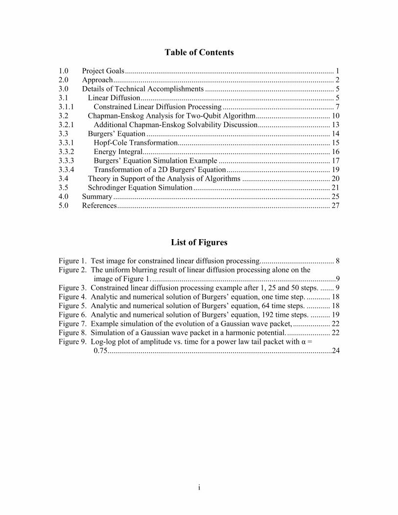
1.0 Project Goals........................................................................................................... 1 2.0 Approach................................................................................................................. 2 3.0 Details of Technical Accomplishments .................................................................. 5 3.1 Linear Diffusion................................................................................................... 5 3.1.1 Constrained Linear Diffusion Processing ......................................................... 7 3.2 Chapman-Enskog Analysis for Two-Qubit Algorithm...................................... 10 3.2.1 Additional Chapman-Enskog Solvability Discussion..................................... 13 3.3 Burgers’ Equation .............................................................................................. 14 3.3.1 Hopf-Cole Transformation.............................................................................. 15 3.3.2 Energy Integral................................................................................................ 16 3.3.3 Burgers’ Equation Simulation Example ......................................................... 17 3.3.4 Transformation of a 2D Burgers' Equation..................................................... 19 3.4 Theory in Support of the Analysis of Algorithms ............................................. 20 3.5 Schrodinger Equation Simulation...................................................................... 21 4.0 Summary ............................................................................................................... 25 5.0 References............................................................................................................. 27

List of Figures

Figure 1. Test image for constrained linear diffusion processing...................................... 8 Figure 2. The uniform blurring result of linear diffusion processing alone on the

image of Figure 1. ..............................................................................................9 Figure 3. Constrained linear diffusion processing example after 1, 25 and 50 steps. ....... 9 Figure 4. Analytic and numerical solution of Burgers’ equation, one time step. ............ 18 Figure 5. Analytic and numerical solution of Burgers’ equation, 64 time steps. ............ 18 Figure 6. Analytic and numerical solution of Burgers’ equation, 192 time steps. .......... 19 Figure 7. Example simulation of the evolution of a Gaussian wave packet, ................... 22 Figure 8. Simulation of a Gaussian wave packet in a harmonic potential. ...................... 22 Figure 9. Log-log plot of amplitude vs. time for a power law tail packet with α =

0.75...................................................................................................................24

1

1.0 Project Goals Our research investigated the feasibility of performing image enhancement, based upon diffusion processing, on a purely quantum or hybrid classical-quantum computer. In the case of hybrid computing using quantum lattice gas algorithms, the approach provides a technological road map for reaching quantum-only computing. A hybrid classical-quantum processor could provide an interim implementation wherein additional qubits could be inserted into the nodes of the lattice and other improvements such as error correction added. In this way, hybrid classical-quantum computing could serve as a testbed for a given hardware approach. In recent years, image processing based upon solving partial differential equations (PDEs) [perona, lions, sapiro, osher] has become more prevalent and developed. These techniques include digital image enhancement and multi-scale image representation by way of nonlinear PDEs. We are motivated to examine these techniques because the fundamental equation of non-relativistic quantum mechanics, the Schrodinger equation, may be viewed as diffusion (or heat conduction) in imaginary time, and diffusion in particular provides a type of digital image filtering. Quantum lattice gas algorithms are able to simulate a variety of PDEs [yepez], including the Navier-Stokes, Boltzmann, and Dirac equations [ibb]. In our research, we investigated which diffusion and related Schrodinger equations may be simulated with a quantum lattice gas algorithm (QLGA). Additionally, we investigated how a QLGA could be extended to perform selective image smoothing in support of image enhancement.

2

2.0 Approach In the mathematical sense, the partial differential equations we simulated with QLGAs are evolution equations of the form ut = f(u,ux,uxx), (2.1) where the subscripts denote partial differentiation, for example, ut ≡ ∂u/∂t. Therefore, we solved equations that are first order in time and second order in space. The PDE is supplemented by an initial condition u(x,t = 0) = u(x,0) and boundary conditions at the endpoints of the x-interval to completely specify the problem. We used periodic boundary conditions, so that for a one-dimensional problem on an interval of length L, u(0,t) = u(L,t). For image processing applications in particular, the dependent variable u corresponds to pixel intensities. For heat transfer problems, u represents the temperature, while for fluid flow problems u corresponds to either the mass density or flow velocity. A quantum lattice gas algorithm is a quantum version of a classical lattice gas, which in turn is an extension of classical cellular automata [yepez, doolen]. In place of the binary lattice variables of a classical lattice gas, the quantum version has a local Hilbert space describing the quantum bit (qubits). In the classical case, in order to recover the proper macroscopic dynamics (and thermodynamics); it is important to ensure that the microscopic dynamics preserves conservation laws. Similarly, in the quantum case, the number densities of qubits must be preserved so that the interaction operator, called the collision operator, must be unitary. The operation of a type-II quantum processor includes the sequential repetition of three main steps [berman, yepez, vahala, love]. First, initialization creates the quantum-mechanical initial state that corresponds to the initial probability distribution for a partial differential equation to be solved. Secondly, a unitary transformation (collision operator) is applied in parallel to all the local Hilbert spaces in the lattice. Lastly, in the measurement step, the quantum states of all the nodes are read out. These results are used to reinitialize the quantum processor in the state which corresponds to the new probability distribution. After the initialization step, a quantum lattice gas algorithm performs iterations of a collision operator and a streaming operator. The latter operator shifts the state of a qubit from a given lattice site to its nearest neighbors in the lattice. It turns out that both of the streaming and collision operations in a QLGA may be combined into a single discretized lattice-Boltzmann equation (LBE) fa(x+εlea,t+ε2τ) – fa(x,t) = Ωa(x,t), (2.2) where Ωa(x,t) = ψ⟨(x,t)|UtnaU – na|ψ(x,t)⟩ is the collision term. Here ea denotes the lattice direction for streaming of qubit a, l is the lattice spacing, τ the time increment, and na the

3

multi-qubit number operator. The small parameter ε is the ratio of l to L, the size of the 1D system, and corresponds physically to the Knudsen number of fluid dynamics. The fa equation above is an analog of the discretized classical Boltzmann equation for a particle distribution function f(x,v,t). The collision term vanishes when U|ψ(x,t)⟩ = |ψ(x,t)⟩. This gives the equilibrium distribution fa

eq. The collision operator U is further constrained by imposing the analog of mass and momentum conservation. These conditions also constrain the collision terms Ωa. For the mass density ρ = ∑a=1

B mafa(x,t) to be constant, we see by multiplying the LBE by ma and summing over the B qubits that ∑a=1

B maΩa(x,t) = 0. (2.3) Similarly, multiplying the LBE by cmaeai, where c is a constant speed, and summing gives c∑a=1

B maeaiΩa(x,t) = 0. (2.4) This represents momentum conservation in the ith direction. Parallel to the mass density ρ = ∑a=1

B mafa is the momentum density ρvi = c∑a=1

B maeaifa(x,t). (2.5) In enforcing mass and momentum conservation we are effectively taking moments of the lattice Boltzmann equation to derive macroscopic quantities for the lattice gas system. In quantum mechanical (QM) terms, the conserved quantities have corresponding operators that commute with the collision operator U. For instance, the mass operator is given by Q0 = ∑a=1

B mana. Then ∑a=1B ma Ωa(x,t) = ψ⟨(x,t)|UtQ0U – Q0|ψ(x,t)⟩ = 0, as previously

described for the equilibrium condition. On the theoretical side of our efforts, we made advances in both deriving finite difference approximations for n-dimensional linear diffusion and in the so-called Chapman-Enskog analysis of simpler QLGAs. For multidimensional anisotropic linear diffusion we now have a QLGA based upon two qubits per node with theory and simulation verifying the form of the diffusion coefficients. We have made progress in developing the Chapman-Enskog multi-scale expansion for 1D QLGAs with two qubits per node. This type of expansion requires a detailed study of the associated equilibrium state of the system, requires the enforcement of mass and momentum conservation, and the pseudo inversion of a Jacobian matrix. The Chapman-Enskog expansion is carried out in the small parameter ε that corresponds to the classical

4

Knudsen number. For our QLGAs, this corresponds to the ratio of the lattice spacing l to the number of nodes. The Jacobian matrix is a result of linearizing the right-side of the lattice Boltzmann equation with the collision operator. It is in general a rank deficient matrix, reflecting the imposition of conservation rules. The Chapman-Enskog analysis tends to be rather involved, even for simpler 1D algorithms. It additionally includes algebraic inversions for the equilibrium occupation probabilities. A later section of this report details the Chapman-Enskog analysis for a specific 1D algorithm with two qubits per node and corresponding to unit mass particles, ma = 1, for a = 1 and 2. Under the next heading of this report, we present details first for simulation of the linear diffusion equation and then for Burgers’ nonlinear equation. Further details may be found in an accompanying manuscript that has been submitted for external publication. The discussion for the linear diffusion equation includes the instance of an in-depth Chapman-Enskog analysis. We then proceed to a description of QLGA simulation for the linear and nonlinear Schrodinger equations.

5

3.0 Details of Technical Accomplishments

3.1 Linear Diffusion Diffusion processing has proved very useful for practical image enhancement, wherein the visual quality of an image is improved. We have investigated methods of carrying out such processing in a combined classical-quantum computing environment. While quantum Fourier and some quantum wavelet transforms are known [nielsen], their direct application to image or signal processing is unclear. Motivated by real-world applications, we offer an alternative based upon the simulation of PDEs. Key to the efficient simulation of PDEs on a hybrid (or Type II) processor is the execution of a QLGA. In a type-II architecture, nodes of phase-coherent, entangled qubits are linked by classical communication to nearest neighbors in a discrete lattice [yepez, yepez01]. Generally this type-II approach has the advantage of requiring both less spatial and temporal entanglement than for the usual (type-I) quantum computing methods. Indeed, if the coherence time of the qubits should be sufficiently long, quantum error correction would not be required. However, such error correction could be implemented within the nodes if needed, or as a testbed of an interim quantum computing (QC) technology. A QLGA includes the sequential repetition of three main steps [yepez, yepez01, berman, vahala, yepez06]. First, initialization creates the quantum-mechanical initial state that corresponds to the initial probability distribution for a partial differential equation to be solved. Secondly, a unitary transformation is applied in parallel to all the local Hilbert spaces in the lattice. Lastly, in the measurement step, the quantum states of all the nodes are read out. These results are used to reinitialize the QC in the state which corresponds to the new probability distribution. The type-II approach offers a means to effectively solve complex gas and fluid dynamics problems [yepez, vahala]. While QLGAs have been shown to solve a number of PDEs, implementation of these algorithms has been mainly done for one spatial dimension only. Very recently multi-dimensional simulation for the Schrodinger equation has been performed [sakai]. Classical lattice Boltzmann simulations have proved highly valuable for fluid phenomenon, including the presence of complex geometry. Quantum lattice gas algorithms may be written in an analogous discretized lattice Boltzmann equation form as mentioned in Section 2.0. There exist quantum lattice gas algorithms that do not correspond to the average over some underlying lattice-gas model in the Boltzmann approximation and their complexity analysis remains an open problem [love]. The algorithms we consider do have a classical counterpart and these provide an efficient implementation on parallel architectures. Therefore our work highly suggests the usefulness of both classical and hybrid classical-

6

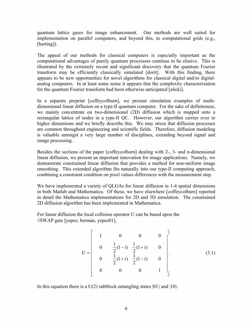
quantum lattice gases for image enhancement. Our methods are well suited for implementation on parallel computers, and beyond this, to computational grids (e.g., [harting]). The appeal of our methods for classical computers is especially important as the computational advantages of purely quantum processors continue to be elusive. This is illustrated by the extremely recent and significant discovery that the quantum Fourier transform may be efficiently classically simulated [dorit]. With this finding, there appears to be new opportunities for novel algorithms for classical digital and/or digital-analog computers. In at least some sense it appears that the complexity characterization for the quantum Fourier transform had been otherwise anticipated [alicki]. In a separate preprint [coffeycolburn], we present simulation examples of multi-dimensional linear diffusion on a type-II quantum computer. For the sake of definiteness, we mainly concentrate on two-dimensional (2D) diffusion which is mapped onto a rectangular lattice of nodes in a type-II QC. However, our algorithm carries over to higher dimensions and we briefly describe this. We may stress that diffusion processes are common throughout engineering and scientific fields. Therefore, diffusion modeling is valuable amongst a very large number of disciplines, extending beyond signal and image processing. Besides the sections of the paper [coffeycolburn] dealing with 2-, 3- and n-dimensional linear diffusion, we present an important innovation for image applications. Namely, we demonstrate constrained linear diffusion that provides a method for non-uniform image smoothing. This extended algorithm fits naturally into our type-II computing approach, combining a constraint condition on pixel values differences with the measurement step. We have implemented a variety of QLGAs for linear diffusion in 1-4 spatial dimensions in both Matlab and Mathematica. Of these, we have elsewhere [coffeycolburn] reported in detail the Mathematica implementations for 2D and 3D simulation. The constrained 2D diffusion algorithm has been implemented in Mathematica. For linear diffusion the local collision operator U can be based upon the √SWAP gate [yepez, berman, yepez01],

.

1000

0)1(21)1(

210

0)1(21)1(

210

0001

⎥⎥⎥⎥⎥⎥⎥⎥

⎦

⎤

⎢⎢⎢⎢⎢⎢⎢⎢

⎣

⎡

−+

+−=

ii

iiU (3.1)

In this equation there is a U(2) subblock entangling states |01⟩ and |10⟩.

7

A preliminary implementation of a type-II QC has been made in a liquid-state nuclear magnetic resonance (NMR) system [pravia]. These experiments used a chloroform (13CHCl3) solution, with hydrogen and a particular carbon nuclei serving as two qubits per node. Sixteen nodes of a one-dimensional lattice were created by the magnetic field of a gradient coil. Specific radio frequency (rf) pulses were applied for the unitary operations on qubits. It was possible to carry out a dozen time steps of the algorithm for the linear 1D diffusion equation. Improved system control should permit the execution of the algorithm for longer times with more fidelity. The NMR ensemble computing approach provides a fascinating combination of quantum computing with classical molecular computing and it has been estimated that implementations with 30 or more addressable qubits would exceed the computational capacity of any classical digital computer (e.g., [love]). Many further avenues for physical implementations of type-II QCs should exist. These include other spin-based systems, coupled ion or neutral atom traps, and flux-, charge-, or phase-based superconducting qubit systems [berns]. An attraction of the type-II approach is the possibility of realization significantly prior to large-scale type-I QCs.

3.1.1 Constrained Linear Diffusion Processing To be of most use to image processing tasks, we would like to have the ability to perform selective image smoothing and linear diffusion alone will not provide this. In this subsection we describe and demonstrate a technique that gives non-uniform image smoothing within our type-II computing approach. We combine a linear diffusion step with a constraint condition step. Since measurement of qubit states is part of a quantum lattice gas algorithm, the incorporation of the constraint step fits well as part of the overall algorithm. An example of the use of constrained linear diffusion for color image dequantization with classical computing is given in [keysers]. Suppose that our original image is I0. We now perform at iteration j, j = 1,2,… on image Ij: (i) 2D linear diffusion, giving the image Ij', followed by (ii) the pixelwise constraint Ij+1(x,y) = max[I0(x,y) - δ, min(I0(x,y) + δ, Ij'(x,y))]. (3.2) Here δ is a processing parameter. It can be chosen according to the distribution of pixel values or other properties of an image. For instance, δ can be taken as proportional to the quantization level for pixel intensities. For gray scale images with pixel values in the range 0 to 28-1 we could choose δ∝ 2-8. Note that the measurement and constraint step in the above algorithm effectively gives us a form of nonlinear operation within the processing. This is an advantage of the type-II computing approach. With a pure quantum processor, this would not be possible. With the constraint in place, image regions with similar pixel intensities are diffused while

8

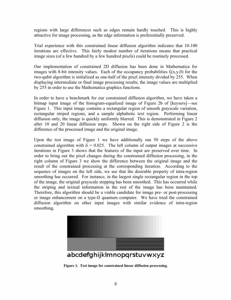
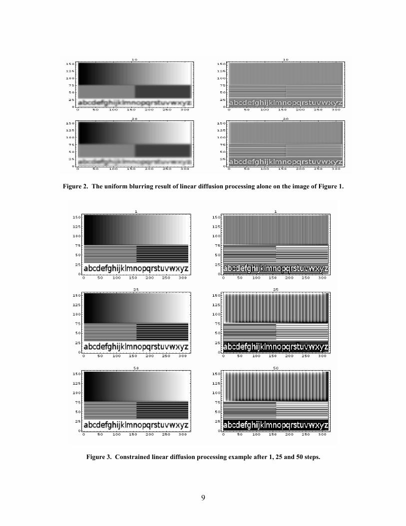
regions with large differences such as edges remain hardly touched. This is highly attractive for image processing, as the edge information is preferentially preserved. Trial experience with this constrained linear diffusion algorithm indicates that 10-100 iterations are effective. This fairly modest number of iterations means that practical image sizes (of a few hundred by a few hundred pixels) could be routinely processed. Our implementation of constrained 2D diffusion has been done in Mathematica for images with 8-bit intensity values. Each of the occupancy probabilities fj(x,y,0) for the two-qubit algorithm is initialized as one-half of the pixel intensity divided by 255. When displaying intermediate or final image processing results, the image values are multiplied by 255 in order to use the Mathematica graphics functions. In order to have a benchmark for our constrained diffusion algorithm, we have taken a bitmap input image of the histogram-equalized image of Figure 2b of [keysers]—see Figure 1. This input image contains a rectangular region of smooth grayscale variation, rectangular striped regions, and a sample alphabetic text region. Performing linear diffusion only, the image is quickly uniformly blurred. This is demonstrated in Figure 2 after 10 and 20 linear diffusion steps. Shown on the right side of Figure 2 is the difference of the processed image and the original image. Upon the test image of Figure 1 we have additionally run 50 steps of the above constrained algorithm with δ = 0.025. The left column of output images at successive iterations in Figure 3 shows that the features of the input are preserved over time. In order to bring out the pixel changes during the constrained diffusion processing, in the right column of Figure 3 we show the difference between the original image and the result of the constrained processing at the corresponding iteration. According to the sequence of images on the left side, we see that the desirable property of intra-region smoothing has occurred. For instance, in the largest single rectangular region in the top of the image, the original grayscale stepping has been smoothed. This has occurred while the striping and textual information in the rest of the image has been maintained. Therefore, this algorithm should be a viable candidate for image pre- or post-processing or image enhancement on a type-II quantum computer. We have tried the constrained diffusion algorithm on other input images with similar evidence of intra-region smoothing.

Figure 1. Test image for constrained linear diffusion processing.

9

Figure 2. The uniform blurring result of linear diffusion processing alone on the image of Figure 1.

Figure 3. Constrained linear diffusion processing example after 1, 25 and 50 steps.

10

Figure 3 is an example of constrained linear diffusion processing. The images in Figure 3 show the results after 1, 25, and 50 steps. With a constraint step (on pixel value differences) included in the overall algorithm, the edge information within the image is maintained. By way of summary and emphasis, we may state that within the constrained diffusion processing approach, we effectively achieve nonlinear filtering of a signal or image, without the much greater complexity of solving a nonlinear diffusion equation. The constrained linear diffusion algorithm contains a parameter δ for pixel wise comparison of the intensities of the current with the previous and original images. We also investigated other variations on constrained linear diffusion, including the choice and possible adaptivity of the constraint parameter δ.

3.2 Chapman-Enskog Analysis for Two-Qubit Algorithm In this section we describe the Chapman-Enskog analysis for a QLGA for linear diffusion with two qubits per node. Suppose that the lattice Boltzmann equation takes the form

fa(x+εlea,t+ε2τ) – fa(x,t) = Ωa(x,t), (3.3) where l is the lattice spacing, ea the momentum directions for the particles (ath qubit), τ the time step, and Ωa the collision term. For this relatively simple example, a = 1, 2 only and e1 = 1, e2 = -1. The occupancy probabilities fa give the probability amplitudes for each of the two qubits as

|qa(x,t)⟩ = √fa(x,t)}|1⟩ + √(1-fa(x,t))|0⟩. (3.4) The (small) expansion parameter ε ~ l/L, where L gives the size of the 1D system, corresponds to the classical Knudsen number. (l serves as the mean free path between collisions here.) In this case the collision terms may be written as Ω1 = -Ω2 = Ω, where Ω = ½[f2(1-f1) - f1(1-f2)]. (3.5) They satisfy Ω1 + Ω2 = 0, corresponding to mass density conservation for unit mass particles. We may note that the Jacobian matrix Jab = ∂Ωa /∂fb,

,11

1121

⎟⎟⎠

⎞⎜⎜⎝

⎛−

−=J (3.6)

is independent of the occupational probabilities fa. Equilibrium occurs for Ωa = 0 or f1 = f2 = d/2. The Jacobian is a special case of a Hermitian matrix. Its two Eigen values must be real and their sum λ1 + λ2 = -1 = Tr J, where Tr denotes the trace operation.

11

Taylor series expanding equation (3.3) gives

...)()(2

32

222

2 +∂Ω∂

Σ+Ω=+∂∂

+∂∂

+∂∂

bb

bbaa

za

aaa f

ffO

xfel

tf

xf

le δεετεε (3.7)

where ea

2 = 1 and … represent higher order terms. For the Chapman-Enskog expansion we take f1=f1

(0) + ε f1(1) + ε2 f1

(2) + …, (3.8a) and f2 = f2

(0) + ε f2(1) + ε2 f2

(2) + …, (3.8b) where f1

(0) and f2(0) are the equilibrium values of the occupancy probabilities. Here they

are particularly simple and each given by d/2. The first term of the right side of equation (4) vanishes when evaluated at equilibrium. In this two-qubit example, much of the full Chapman-Enskog analysis may be avoided. We first sum equation (4) over a =1, 2 and use the mass density ρ = f1+f2, giving

.02

)( 2

2222

21 =∂∂

+∂∂

+−∂∂

xl

tff

xl ρερτεε (3.9)

Here we interchanged the double sum on the right side and applied conservation of mass. It appears that the first term on the left side of equation (3.9) also contributes at O(ε2) and we proceed to work out the details for ε(f1

(1) - f2(1)). Consider the O(ε) equations from

equation (4). Explicitly these read

)1()0(

bb

ab

aa f

fxf

le∂Ω∂

Σ=∂∂

. (3.10)

By making use of the Jacobian matrix of equation (3.6) these equations are:

],[21 )1(

1)1(

2

)0(1 ffx

fl −=∂∂ (3.11a)

and

].[21 )1(

2)1(

1

)0(2 ffx

fl −=∂∂

− (3.11b)

Summing equations (3.11a) and (3.11b) gives: l(∂/∂x) (f1

(0) - f2(0)) = 0. (3.12)

12

This is expected since f1(0) = f2

(0). This consistency check is a special case of a much more general solvability condition corresponding to general equations of the form of equation (3.10) and is further discussed in the Appendix. The solvability condition arises due to the fact that the Jacobian matrix J appearing in equation (3.10) is not invertible. Equation (3.10) may also be written in matrix-vector form

,|| )1()0(

>>=∂∂

fJx

fel a

a (3.13)

where: |f(1)⟩ = .)1(2

)1(1⎥⎦

⎤⎢⎣

⎡

ff

The Jacobian has two Eigen values λ1 = 0 and λ2 = -1 with (right)

Eigen vectors (1,1)T and (-1,1)T respectively, where T denotes transposition. Note that J2 = - J = λ2 J. So multiplying equation (3.13) on the left by J gives

.|| )1(2

)0(

>>=∂∂

fJx

felJ a

a λ (3.14)

We take this equation to imply l |ea (∂fa

(0)/∂x)⟩ = λ2 |f(1)⟩, (3.15) omitting discussion of the pseudo inverse of a matrix. Component wise, equation (3.15) states that l (∂f1

(0)/∂x) = -f1(1), (3.16a)

-l (∂f2

(0)/∂x) = -f2(1), (3.16b)

i.e., the first order corrections f1

(1) and f2(1) are directly proportional to the derivative (the

gradient in higher dimensions) of the corresponding equilibrium distribution. Now consider the (first nonzero) contribution at O(ε2) from the first term on the left side of equation (3.9) that we may identify from:

⎥⎦

⎤⎢⎣

⎡+

∂∂

+∂∂

+∂∂

Σ=∂∂

Σ ...)2(

2)1()0(

xf

xf

xf

elxf

el aaaaa

aaa εεεε (3.17a)

⎥⎦

⎤⎢⎣

⎡+

∂∂

+∂∂

Σ= ...)2()1(

2

xf

xf

el aaaa εε (3.17b)

13

⎥⎦

⎤⎢⎣

⎡+

∂∂

Σ+∂∂

−∂∂

= ...)2()1(

2)1(

12

xf

xf

xf

l aaεε (3.17c)

⎥⎦

⎤⎢⎣

⎡+

∂∂

−∂

∂−= )(2

)0(2

2

2

)0(1

22 εε O

xf

lxf

ll (3.17d)

.)(2

22

⎥⎦

⎤⎢⎣

⎡+

∂∂

−= ερε Ox

ll (3.17e)

Here equation (3.17b) follows from equation (3.17a) by momentum conservation (or, equivalently, by equation (3.12)). Equation (3.17d) follows from equation (3.17c) by applying the relations (3.16). We conclude that

.)()( 2

222

21 ⎥⎦

⎤⎢⎣

⎡+

∂∂

−=−∂∂

=∂∂

Σ ερεεε Ox

lffx

lxf

el aaa (3.18)

Then equation (3.9) becomes (at O(ε2))

,0121

2

22 =

∂∂

⎟⎠⎞

⎜⎝⎛ −+

∂∂

tl

tρρτ (3.19a)

or

,2 2

22

tl

t ∂∂

⎟⎟⎠

⎞⎜⎜⎝

⎛=

∂∂ ρ

τρ (3.19b)

the linear diffusion equation with diffusion constant D = l2/2τ.

3.2.1 Additional Chapman-Enskog Solvability Discussion We further discuss the solvability condition for the first order equations (3.10) and the null Eigen vectors of the Jacobian matrix. We assume B qubits. The mass density conservation condition for the collision terms is ∑a=1

B maΩa({fj}) = 0. Hence, expanding about equilibrium, fa = fa

(0) + ε fa(1), we have the condition ∑a,b ma Jab

fb(1) = 0 where fb

(1) is arbitrary. Thus the vector ⟨M| = (m1,m2,…,mB) is a left null Eigen vector of J, ⟨M|J = 0. Multiplying equation (3.10) on the left by ⟨M| we obtain the solvability condition l∑a ea ma ∂fa

(0)/∂x = 0. For the equal-mass, two-qubit example above, this equation is trivially satisfied.

14

The momentum density conservation condition for the collision terms is ∑a=1B ma

eaΩa({fj}) = 0. Expanding about equilibrium, we obtain the condition ∑a,b ma ea Jab fb(1) =

0 where again fb(1) is arbitrary. This equation implies ⟨u| = (m1e1,…,mBeB) is also a left

null Eigen vector of J. This condition does not hold for the one dimensional two-qubit example above where the average momentum is zero. The Jacobian matrix of equation (3.6) is special in another sense. It is an example of a symmetric circulant matrix, for which Jab = j|a-b|, where jc is a vector of coefficients. Since this operator is real and symmetric, it has only real Eigen values. For the QLGAs, J is generally rank deficient and so has at least one zero Eigen value. Since the entries of Jab depend only upon the difference a - b, J is also a Toeplitz matrix. Very many results are known on the Eigen structure of Toeplitz and circulant matrices. Typically for QLGAs, the coefficients of jc are highly related and multiple zero digenvalues result. A reference for the Chapman-Enskog expansion for classical computational fluid dynamics is the book Lattice-gas Cellular Automata by D. H. Rothman and S. Zaleski, Cambridge University Press (1997). (See especially Ch. 15.)

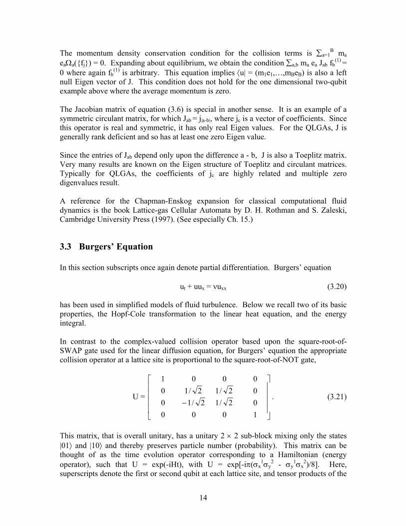
3.3 Burgers’ Equation In this section subscripts once again denote partial differentiation. Burgers’ equation ut + uux = νuxx (3.20) has been used in simplified models of fluid turbulence. Below we recall two of its basic properties, the Hopf-Cole transformation to the linear heat equation, and the energy integral. In contrast to the complex-valued collision operator based upon the square-root-of-SWAP gate used for the linear diffusion equation, for Burgers’ equation the appropriate collision operator at a lattice site is proportional to the square-root-of-NOT gate,

U =

⎥⎥⎥⎥

⎦

⎤

⎢⎢⎢⎢

⎣

⎡

−100002/12/1002/12/100001

. (3.21)

This matrix, that is overall unitary, has a unitary 2 × 2 sub-block mixing only the states |01⟩ and |10⟩ and thereby preserves particle number (probability). This matrix can be thought of as the time evolution operator corresponding to a Hamiltonian (energy operator), such that U = exp(-iHt), with U = exp[-iπ(σx

1σy2 - σy

1σx2)/8]. Here,

superscripts denote the first or second qubit at each lattice site, and tensor products of the

15

Pauli spin matrices σj are implicit in the notation, e.g., σx1σy

2 = σx1 ⊗ σy

2. The collision operator for the entire lattice is a L-fold tensor product over the local collision operators, C = ⊗j=0

L-1 U.

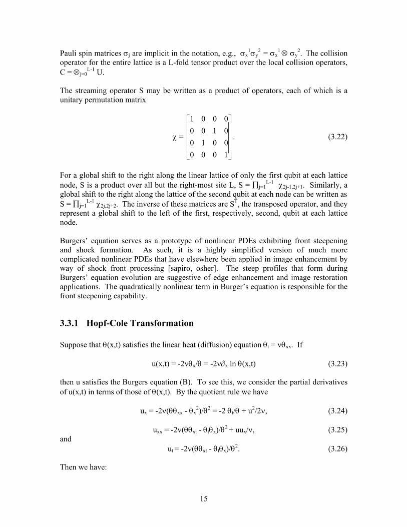
The streaming operator S may be written as a product of operators, each of which is a unitary permutation matrix

χ =

⎥⎥⎥⎥

⎦

⎤

⎢⎢⎢⎢

⎣

⎡

1000001001000001

. (3.22)

For a global shift to the right along the linear lattice of only the first qubit at each lattice node, S is a product over all but the right-most site L, S = ∏j=1

L-1 χ2j-1,2j+1. Similarly, a global shift to the right along the lattice of the second qubit at each node can be written as S = ∏j=1

L-1 χ2j,2j+2. The inverse of these matrices are ST, the transposed operator, and they represent a global shift to the left of the first, respectively, second, qubit at each lattice node. Burgers’ equation serves as a prototype of nonlinear PDEs exhibiting front steepening and shock formation. As such, it is a highly simplified version of much more complicated nonlinear PDEs that have elsewhere been applied in image enhancement by way of shock front processing [sapiro, osher]. The steep profiles that form during Burgers’ equation evolution are suggestive of edge enhancement and image restoration applications. The quadratically nonlinear term in Burger’s equation is responsible for the front steepening capability.

3.3.1 Hopf-Cole Transformation Suppose that θ(x,t) satisfies the linear heat (diffusion) equation θt = νθxx. If u(x,t) = -2νθx/θ = -2ν∂x ln θ(x,t) (3.23) then u satisfies the Burgers equation (B). To see this, we consider the partial derivatives of u(x,t) in terms of those of θ(x,t). By the quotient rule we have ux = -2ν(θθxx - θx

2)/θ2 = -2 θt/θ + u2/2ν, (3.24) uxx = -2ν(θθxt - θtθx)/θ2 + uux/ν, (3.25) and ut = -2ν(θθxt - θtθx)/θ2. (3.26) Then we have:

16

ut + uux = -2νθxt/θ + 2ν(θx/θ)(θt/θ) + uux = -2νθxt/θ -u(θt/θ) + uux. (3.27) We compare to the expression: νuxx = -2νθxt/θ + 2ν(θx/θ)(θt/θ) + uux= -2νθxt/θ -u(θt/θ) + uux. (3.28) Therefore we have verified that ut + uux = νuxx, where the parameter ν is physically a scaled kinematic viscosity. We may note from equation (3.23) that by integrating, ln θ(x,t) = -(1/2ν)∫x u(x’,t)dx’ and θ(x,t) = C(t) exp[-(1/2ν)∫xx0 u(x’,t)dx’], (3.29) with C(t) = θ(x0,t). The latter relation follows simply from θ(x0,t) = C(t) exp(0). Similarly the initial values of u and θ are related. If u(x,0) = u0(x), then θ(x,0) = θ0(x) = C0 exp[-(1/2ν)∫xx0 u0(x’)dx’]. (3.30) If the linear diffusion equation is solved on the whole x axis, then one way to represent θ(x,t) is as a convolution of the initial condition θ0(x) with a Gaussian function with variance given by 2νt. Then applying the Hopf-Cole transformation (3.23) gives the solution u(x,t) of the Burgers’ equation. Using vector notation it is possible to write higher dimensional and vector analogs of the Burgers’ equation and the Hopf-Cole transformation. With ∇ the gradient operator in n dimensions, the 1D Burgers’ equation generalizes to qt + q⋅∇q = ν∇2q. (3.31) If θ(x,t) satisfies the linear diffusion equation θt = ν∇2θ, then q(x,t) = -2ν∇ln θ(x,t) (3.32) satisfies the n-dimensional Burgers’ equation.

3.3.2 Energy Integral Suppose that we multiply Burgers’ equation (B) by u, uut + u2ux = νuuxx, (3.33) and then recognize certain derivatives:

17

½ ∂tu2 + (1/3) ∂xu3 = -νux2 + ν∂x(uux). (3.34)

Integrating this equation with respect to x from x1 to x2 gives the relation

(1/2)∂t ∫x2x1 u2(x,t)dx + (1/3) [u3(x2,t) – u3(x1,t)]

= -∫x2x1 u2

x(x,t)dx + ν[u(x2,t)ux(x2,t) – u(x1,t)ux(x1,t)]. (3.35) The two terms on the left side of this equation represent the total rate of change of kinetic energy in the system and the net flux of kinetic energy out of the system across the boundaries. The two terms on the right side represent the total dissipation of energy by viscosity in the system and the rate of work done on the system at the boundaries. The nonlinear term of Burgers’ equation gives a means of putting energy into the system across the boundaries. We omit any general discussion of scaling properties of the Burgers’ equation, but do note that under the transformation u → -u the Burgers’ equation becomes ut – uux = νuxx, (3.36) i.e., the sign of the nonlinear term is changed. Correspondingly, the Hopf-Cole transformation becomes u(x,t) = 2νθx/θ = 2ν∂x ln θ(x,t). (3.37) Since each term of the Burgers’ equation contains a differentiation, a linear transformation of the dependent variable introduces an additional linear term in the PDE. In particular, if v(x,t) = au(x,t) + b for constants a and b, then v satisfies the modified Burgers’ equation vt + (1/a)(v-b)vx = νvxx. (3.38) This simple property is sometimes useful in solving an initial value problem by bringing a PDE into the standard form of Burgers’ equation.

3.3.3 Burgers’ Equation Simulation Example We tested our implementation of Burgers’ equation simulation with a cosinusoidal initial profile ρ(x,0) = ρa + ρb cos(2πx), (3.39) where ρa = 0.4 and ρb = 1.0. The exact solution for this problem may be based upon a slightly extended version of the Hopf-Cole transformation equation (HC’): ρ(x,t) = ρa + (2ν/c)θx/θ, (3.40)

18

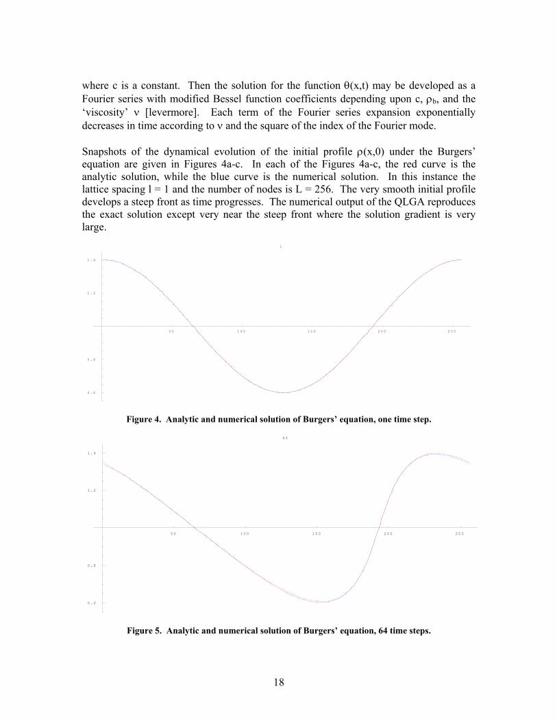
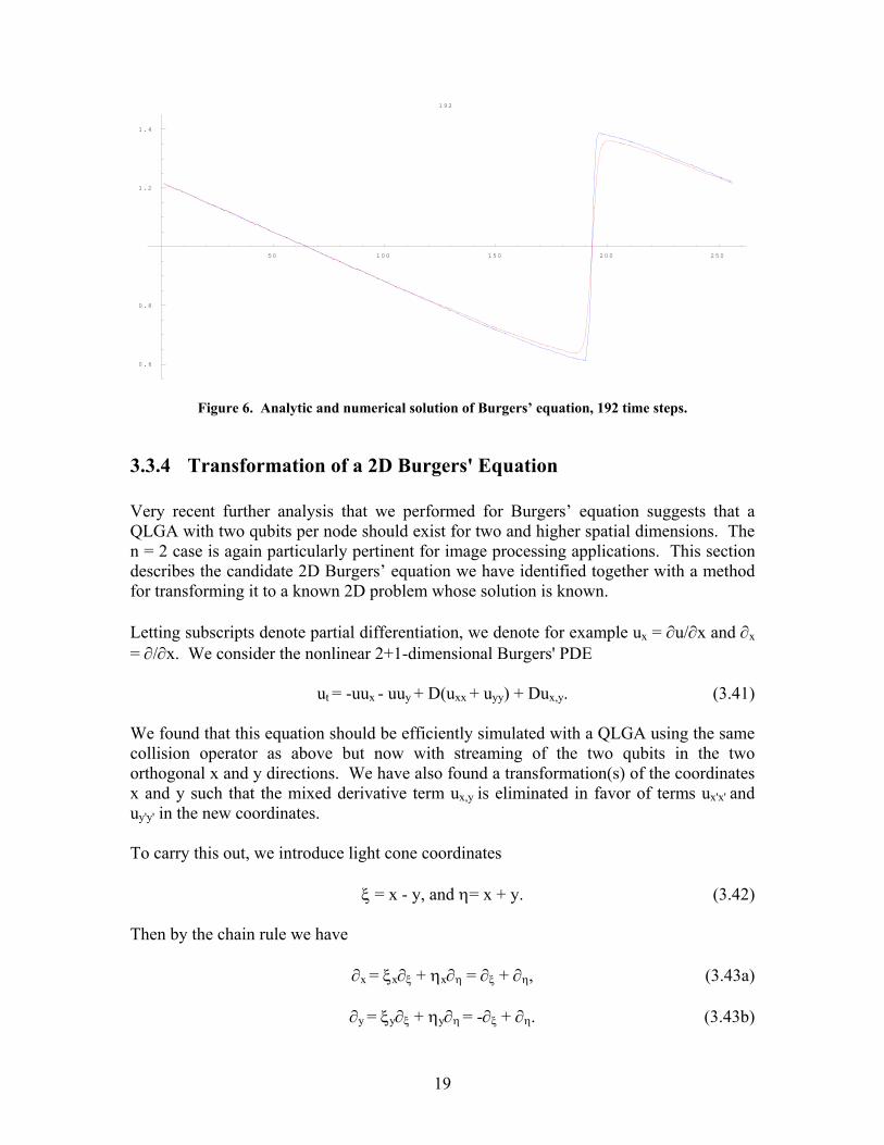
where c is a constant. Then the solution for the function θ(x,t) may be developed as a Fourier series with modified Bessel function coefficients depending upon c, ρb, and the ‘viscosity’ ν [levermore]. Each term of the Fourier series expansion exponentially decreases in time according to ν and the square of the index of the Fourier mode. Snapshots of the dynamical evolution of the initial profile ρ(x,0) under the Burgers’ equation are given in Figures 4a-c. In each of the Figures 4a-c, the red curve is the analytic solution, while the blue curve is the numerical solution. In this instance the lattice spacing l = 1 and the number of nodes is L = 256. The very smooth initial profile develops a steep front as time progresses. The numerical output of the QLGA reproduces the exact solution except very near the steep front where the solution gradient is very large.

5 0 1 0 0 1 5 0 2 0 0 2 5 0

0 . 6

0 . 8

1 . 2

1 . 4

1

Figure 4. Analytic and numerical solution of Burgers’ equation, one time step.

5 0 1 0 0 1 5 0 2 0 0 2 5 0

0 . 6

0 . 8

1 . 2

1 . 4

6 4

Figure 5. Analytic and numerical solution of Burgers’ equation, 64 time steps.

19

50 1 0 0 1 5 0 2 0 0 2 5 0

0. 6

0. 8

1. 2

1. 4

19 2

Figure 6. Analytic and numerical solution of Burgers’ equation, 192 time steps.

3.3.4 Transformation of a 2D Burgers' Equation Very recent further analysis that we performed for Burgers’ equation suggests that a QLGA with two qubits per node should exist for two and higher spatial dimensions. The n = 2 case is again particularly pertinent for image processing applications. This section describes the candidate 2D Burgers’ equation we have identified together with a method for transforming it to a known 2D problem whose solution is known. Letting subscripts denote partial differentiation, we denote for example ux = ∂u/∂x and ∂x = ∂/∂x. We consider the nonlinear 2+1-dimensional Burgers' PDE ut = -uux - uuy + D(uxx + uyy) + Dux,y. (3.41) We found that this equation should be efficiently simulated with a QLGA using the same collision operator as above but now with streaming of the two qubits in the two orthogonal x and y directions. We have also found a transformation(s) of the coordinates x and y such that the mixed derivative term ux,y is eliminated in favor of terms ux'x' and uy'y' in the new coordinates. To carry this out, we introduce light cone coordinates ξ = x - y, and η= x + y. (3.42) Then by the chain rule we have ∂x = ξx∂ξ + ηx∂η = ∂ξ + ∂η, (3.43a) ∂y = ξy∂ξ + ηy∂η = -∂ξ + ∂η. (3.43b)

20

For the 'non-mixed' second derivatives, by operator algebra we have ∂xx = (∂ξ +∂η)2 = ∂ξξ + 2∂ξη + ∂ηη (3.44) ∂yy = (-∂ξ + ∂η)2 = ∂ξξ - 2∂ξη + ∂ηη. (3.45) In particular, for the mixed derivative term we have ∂x ∂y = (∂ξ + ∂η)(-∂ξ + ∂η) = ∂ηη - ∂ξξ. (3.46) By making use of the equations just above in the 2D Burger's equation we obtain ut = -2uuη + D(uξξ + 3uηη). (3.47) This appears to be an anisotropic form of a 2D Burgers' equation very close to that considered by Elton [elton], and Shen et al. [shen], and possibly others in regard to classical lattice gas algorithms. Using different lattice spacings Δx ≠ Δy should accommodate the anisotropy of the second order derivative terms. If necessary, a scaling of the dependent variable u may be used to eliminate the factor of 2 in the 2uuη term. If u(ξ,η) = v(ξ,η)/2, then vt = -vvη + D(vξξ + 3vηη). (3.48)

3.4 Theory in Support of the Analysis of Algorithms Often in the run-time analysis of algorithms alternating binomial sums arise in the determination of the order of operations. In the course of our investigations we were able to make theoretical contributions to this subject of computer science. The theory entails special functions and numbers and combinatorics together with extensive analytic development. The end results are exact, not just asymptotic for a large number of computing operations, as was often the case in the previous literature. They support the design and analysis of algorithms, whether they be classical, purely quantum, or hybrid. Given an alternating binomial sum, the sign alternation in the summand causes substantial cancellation, masking the leading behavior. If S(n) = Σj=0

n (-1)j (nj) f(j), where

(nj) denotes the binomial coefficient, virtually any order in n is realizable, depending upon

the function f. If f = 1, we obtain 0, while if f(j) = (-1)j, we obtain 2n. Therefore, the full range of growth from sub-polynomial in n to exponential in n may result. Typically, otherwise asymptotic results have been sought from the beginning of the analysis. We showed how to exactly calculate a class of binomial sums of interest. In our approach we used a variety of integral representations and special numbers and special functions. Concepts and functions from combinatorial theory are additionally used. Complex-valued functions f are included in the theory. For a recent graduate level

21

textbook on the average case analysis of algorithms, including a treatment of alternating sums, one may see the book of Szpankowski [szpankowski]. Our analytic results are sufficiently general to subsume many other previously known special cases. From these more general results, asymptotic estimates may be obtained if desired. Special cases include a sum useful for computing decoherence factors for a coupled multi-qubit environment and multi-qubit subsystem. Our preprint entitled “A set of identities for a class of alternating binomial sums arising in computing applications” has been accepted for external publication [utilmath].

3.5 Schrodinger Equation Simulation The time-dependent Schrodinger equation (TDSE) can be described by a number of QLGAs, three of which we have implemented and compared. The first is the simplest, proposed by Boghosian and Taylor in their paper on a quantum lattice-gas model in d dimensions [boghosian98]. The other two are improved-accuracy algorithms but with a greater number of operations, proposed by Yepez and Boghosian [yepez02]. These QLGAs do not measure the qubit states after collision and streaming. Therefore, they assume that the entangled qubit states may be reliably retained throughout the length of the simulation. In principle these QLGAs may then obtain exponential speed up over classical simulation of the Schrodinger equation. Because of the necessity to maintain and stream the entangled qubit states over all time steps, the engineering requirements for physical implementation are much more stringent than for QLGAs with occasional or regularly repeated measurement. The Yepez and Boghosian approach uses a combination of streaming qubit states to both left and right neighbors in the case of a one-dimensional lattice. In this way an algorithm more symmetric in the streaming step is obtained and higher accuracy of the solution usually results. Versus four total operations of streaming and collision for the Boghosian and Taylor method, the Yepez and Boghosian approach has eight or sixteen such operations. The papers cited just above provide more details of the QLGAs. The potential energy term V(x) of the Schrodinger equation is introduced by applying a local phase change to the system wave function as [ibb] ψ(x,t) → e-iV(x)τ ψ(x,t). (3.49) Then we obtain equations of the form ih ∂ψ/∂t = (h 2/2m)∂2ψ/∂x2 + V(ψ)ψ, (3.50) that model a quantum particle under the influence of an external force F(x) = -dV(x)/dx. A key point is that we may take the potential to depend upon ψ itself. In this way, we are also able to simulate the nonlinear time-dependent Schrodinger equation. If, for instance, V has a power law nonlinearity of degree n, then the TDSE has nonlinearity of degree n+1. In particular, taking V(ψ) = |ψ|2, we obtain the cubic nonlinear Schrodinger

22

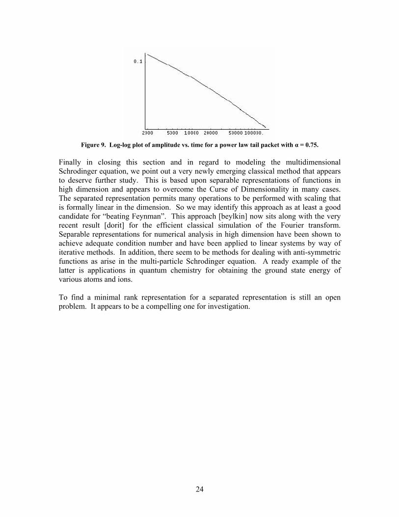
equation. However, the nonlinearities of the potential need not be restricted to power-law form, and this is useful in modeling other physical systems [jordan]. These other nonlinearities include V(ψ) = |ψ|2/(1 + |ψ|2) and V(ψ) = 1- exp(-|ψ|2). We performed TDSE simulations for a variety of problems with and without potential energy term. A first case is given in Figure 7 for a free Gaussian wave packet. In this case the exact solution is known in terms of separation of variables and Fourier series for the spatial dependence. Another well known test case was provided by the harmonic oscillator problem. In Figure 8 the corresponding parabolic potential is shown in green. The spring constant k of the potential was set to 10-5 and the particle mass to 1. The classical period for this wave packet is T = 2π/ω = 2π/√k ≈ 1987 δt, where δt is eight time steps for the Yepez 8-step algorithm. The simulation was run for 80,000 time steps, and the expected five periods of oscillation in the potential were obtained.

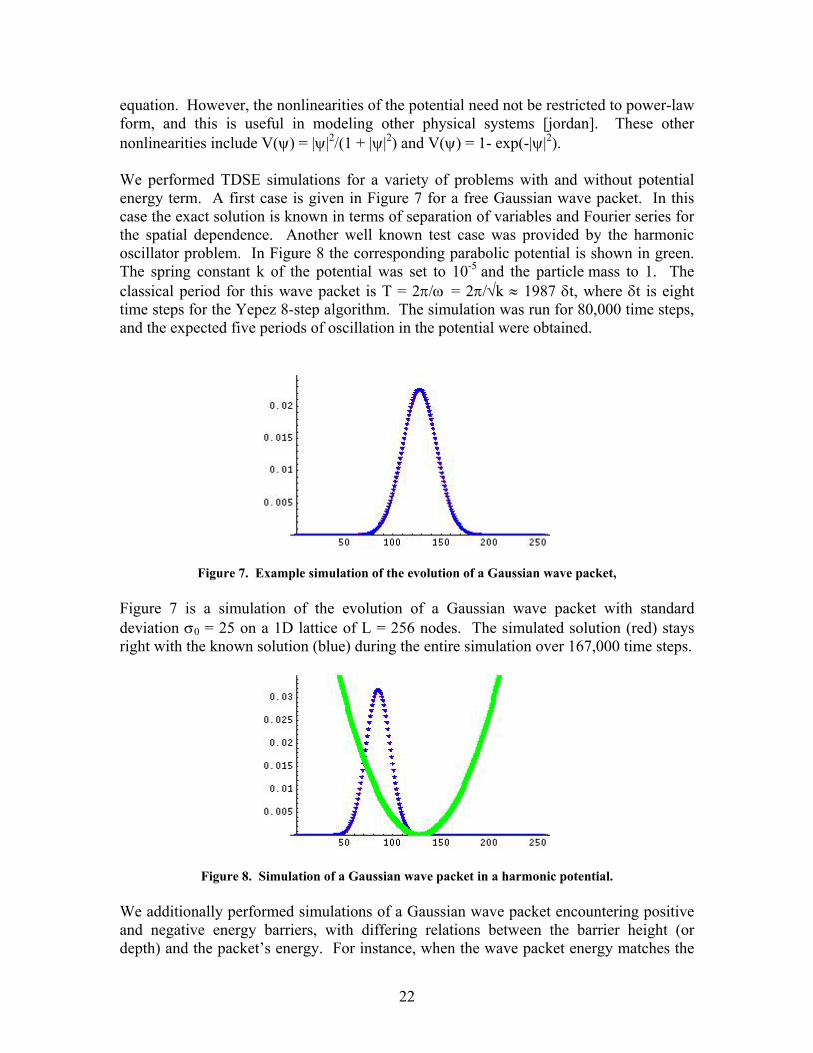
Figure 7. Example simulation of the evolution of a Gaussian wave packet, Figure 7 is a simulation of the evolution of a Gaussian wave packet with standard deviation σ0 = 25 on a 1D lattice of L = 256 nodes. The simulated solution (red) stays right with the known solution (blue) during the entire simulation over 167,000 time steps.

Figure 8. Simulation of a Gaussian wave packet in a harmonic potential. We additionally performed simulations of a Gaussian wave packet encountering positive and negative energy barriers, with differing relations between the barrier height (or depth) and the packet’s energy. For instance, when the wave packet energy matches the

23

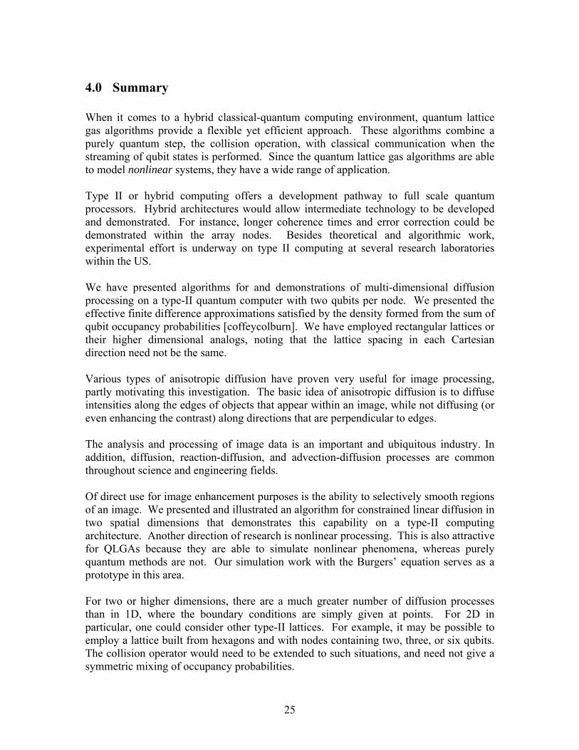
energy level of a repulsive barrier, a sort of resonance occurs. This and other expected behavior emerged from the simulations. We also performed simulations for much more challenging physical systems including power-law wave tail packets (PLTPs) and the Weierstrass-Mandelbrot wave function. PLTPs have received much attention in the literature in the last few years (e.g., [lillo]). A form of them suitable for modeling purposes is ψ(x) = N (x2 + γ2)-α/2, (3.51) where α, γ, and N are constants, with N being the normalization constant. It is possible to explicitly write N as a function of α and γ by evaluating a Beta function integral:

,)()2/1( ααγπ

γ α

Γ−Γ=N (3.52)

where Γ is the Gamma function. We note that for large x, |ψ(x)|2 behaves as |x|-2α. Hence α in the range ½ < α < 3/2 causes the integral (required to find the uncertainty in position)

dxxx 22 |)(|ψ∫∞

∞− (3.53)

to diverge. This means the Heisenberg uncertainty relation, while true, yields no useful information about the uncertainty in momentum or otherwise. In this case, it turns out to be very useful then to investigate entropy-like quantities for the PLTPs. Figure 9 gives an example from a QLGA simulation of a PLTP with α = ¾ run for 150,000 time steps. This figure with log-log scale gives the wave packet amplitude as a function of time. The packet amplitude decreases with time, but not exactly as expected. A normalization check for the packet at the end of the simulation returned N = 0.966 < 1, indicating that some of the packet has been lost off the sides of the lattice due to the imposed periodic boundary condition. This model problem provided a stringent test of the QLGA capabilities. It presented a trade off in the total number of lattice nodes to use, the internal resolution of the wave packet, and the total number of time steps that the quantum evolution could be advanced.

24

Figure 9. Log-log plot of amplitude vs. time for a power law tail packet with α = 0.75.

Finally in closing this section and in regard to modeling the multidimensional Schrodinger equation, we point out a very newly emerging classical method that appears to deserve further study. This is based upon separable representations of functions in high dimension and appears to overcome the Curse of Dimensionality in many cases. The separated representation permits many operations to be performed with scaling that is formally linear in the dimension. So we may identify this approach as at least a good candidate for “beating Feynman”. This approach [beylkin] now sits along with the very recent result [dorit] for the efficient classical simulation of the Fourier transform. Separable representations for numerical analysis in high dimension have been shown to achieve adequate condition number and have been applied to linear systems by way of iterative methods. In addition, there seem to be methods for dealing with anti-symmetric functions as arise in the multi-particle Schrodinger equation. A ready example of the latter is applications in quantum chemistry for obtaining the ground state energy of various atoms and ions. To find a minimal rank representation for a separated representation is still an open problem. It appears to be a compelling one for investigation.

25

4.0 Summary When it comes to a hybrid classical-quantum computing environment, quantum lattice gas algorithms provide a flexible yet efficient approach. These algorithms combine a purely quantum step, the collision operation, with classical communication when the streaming of qubit states is performed. Since the quantum lattice gas algorithms are able to model nonlinear systems, they have a wide range of application. Type II or hybrid computing offers a development pathway to full scale quantum processors. Hybrid architectures would allow intermediate technology to be developed and demonstrated. For instance, longer coherence times and error correction could be demonstrated within the array nodes. Besides theoretical and algorithmic work, experimental effort is underway on type II computing at several research laboratories within the US. We have presented algorithms for and demonstrations of multi-dimensional diffusion processing on a type-II quantum computer with two qubits per node. We presented the effective finite difference approximations satisfied by the density formed from the sum of qubit occupancy probabilities [coffeycolburn]. We have employed rectangular lattices or their higher dimensional analogs, noting that the lattice spacing in each Cartesian direction need not be the same. Various types of anisotropic diffusion have proven very useful for image processing, partly motivating this investigation. The basic idea of anisotropic diffusion is to diffuse intensities along the edges of objects that appear within an image, while not diffusing (or even enhancing the contrast) along directions that are perpendicular to edges. The analysis and processing of image data is an important and ubiquitous industry. In addition, diffusion, reaction-diffusion, and advection-diffusion processes are common throughout science and engineering fields. Of direct use for image enhancement purposes is the ability to selectively smooth regions of an image. We presented and illustrated an algorithm for constrained linear diffusion in two spatial dimensions that demonstrates this capability on a type-II computing architecture. Another direction of research is nonlinear processing. This is also attractive for QLGAs because they are able to simulate nonlinear phenomena, whereas purely quantum methods are not. Our simulation work with the Burgers’ equation serves as a prototype in this area. For two or higher dimensions, there are a much greater number of diffusion processes than in 1D, where the boundary conditions are simply given at points. For 2D in particular, one could consider other type-II lattices. For example, it may be possible to employ a lattice built from hexagons and with nodes containing two, three, or six qubits. The collision operator would need to be extended to such situations, and need not give a symmetric mixing of occupancy probabilities.

26

A concatenated time sequence of images provides a 3D space-time in which to consider image processing. By discriminating changing features in such data, one could detect moving objects. This has potential application to automatic or semi-automatic target recognition. The early NMR experiment which qualitatively demonstrates the feasibility of implementing 1D diffusion [pravia] is encouraging. It provides evidence that the path to large hybrid quantum-classical computers may be realizable well before large-scale type-I quantum computers. In addition, liquid state NMR realizations of an ensemble of sufficient size would exceed the computational capacity of classical digital computers. The various diffusion attributes of dimension, isotropy or anisotropy, forward or backward, and linear or nonlinear processes provide opportunities for designing aspects of image processing on a type-II quantum computing architecture.

27

5.0 References [alicki] R. Alicki, {arXiv:quant-ph/0306103 (2003).} [berggren] K. K. Berggren, {Proc. IEEE 92, 1630 (2004).} [berman] G. P. Berman et al., {Phys. Rev. A 66, 012310 (2002).} [beylkin] G. Beylkin and M. J. Mohlenkamp, SIAM J. Sci. Comp. 26, 2133 (2005). [boghosian98] B. M. Boghosian and W. Taylor, {Phys. Rev. E 57, 54 (1998).} [coffeycolburn] M. W. Coffey and G. G. Colburn, preprint (2006). [cory] Z. Chen, J. Yepez, and D. G. Cory, {quant-ph/0410198 (2004).} [doolen] G. Doolen et al., eds., {Lattice gas methods for partial differential equations, Addison Wesley (1990); G. Doolen, ed., Lattice gas methods: theory, applications, and hardware, MIT Press (1991).} [dorit] D. Aharonov, Z. Landau, and J. Makowsky, {arXiv:quant-ph/0611156 (2006).} [elton] B. H. Elton, {Trans. ACM 242 (1991).} [garb] P. Garbaczeuski, {quant-ph/0408192 (2004).} [garey] M. R. Garey and D. S. Johnson, {Computers and Intractability: A Guide to the Theory of NP-completeness, Freeman, San Francisco (1979); C. H. Papadimitriou, Computational Complexity, Addison Wesley Longman (1994).} [harting] J. Harting et al., {Phil. Trans. Royal Soc. A 363, 1895 (2005).} [hemmer] P. R. Hemmer et al., {quant-ph/007114 (2000).} [ibb] I. Bialynicki-Birula, {Phys. Rev. D 49, 6920 (1994).} [jain] A. Jain, {Fundamentals of digital image processing, Prentice Hall (1995); R. Gonzalez and R. Woods, Digital image processing, Addison Wesley (1993).} [jmodoptics] M. W. Coffey, {J. Mod. Optics, 49, 2389 (2002).} [jordan] R. Jordan and C. Josserand, {Phys. Rev. E 61, 1527 (2000); R. Jordan et al., Physica D 137, 353 (2000).}

28

[keysers] D. Keysers, C. H. Lampert, and T. M. Breuel, {Proc. SPIE El. Imaging (2006).} [klette] R. Klette and P. Zamperoni, {Handbook of image processing operators, John Wiley & Sons (1996).} [koenderink] J. Koenderink, {Biol. Cyb. 50, 363 (1984).} [lillo] F. Lillo and R. N. Mantegna, {Phys. Rev. Lett. 84, 1061 (2000).} [lions] L. Alvarez, P.-L. Lions, and J.-M. Morel, {SIAM J. Num. Anal. 29, 845 (1992); F. Catte et al., SIAM J. Num. Anal. 29, 182 (1992); G.-H. Cottet and L. Germain, Math. Comp. 61, 659 (1993); A. I. El-Fallah and G. E. Ford, SPIE Image and Video Proc. II, 2182, 49 (1994).} [love] P. J. Love and B. M. Boghosian, {quant-ph/0506244, quant-ph/0507022 (2005); Physica A {\bf 362}, 210 (2006).} [massen] S. E. Massen and C. P. Panos, {Phys. Lett. A 346, 530 (1998); Phys. Rev. C 67, 014314 (2003).} [nielsen] M. A. Nielsen and I. L. Chuang, {Quantum Computation and Quantum Information, Cambridge University Press (2000).} [orlando] D. M. Berns and T. P. Orlando, {quant-ph/0401071 (2005).} [osher] S. Osher and N. Paragios, {Geometric level set methods in imaging, vision, and graphics, Springer (2002); S. Osher and L. Rudin, SIAM J. Numer. Analysis 27, 919 (1990).} [panos] C. P. Panos, S. E. Massen, and C. G. Koutroulos, {Phys. Rev. C 63, 064307 (2001).} [perona] P. Perona and J. Malik, {Proc. IEEE Int. Symp. Circuits and Systems, 2565 (1988); Proc. IEEE Comp. Soc. Workshop on Comp. Vision, Miami, FL, p. 16 (1987); IEEE Trans. Patt. Anal. Mach. Intell. 12, 629 (1990).} [pravia] M. Pravia, Z. Chen, J. Yepez, and D. G. Cory, {Comput. Phys. Commun. 146, 339 (2002).} [price] C. B. Price et al., {Iee Proc. 137, 136 (1990); N. K. Nordstrom, Image and Vis. Comp. 8, 318 (1990).} [qcreviews] A. Steane, {Rep. Prog. Phys. 61, 117 (1998); A. Barenco, Contemp. Phys. 37, 375 (1996); A. Ekert and R. Jozsa, Rev. Mod. Phys. 68, 733 (1996); J. Preskill, J. Mod. Opt. 47, 127 (2000); J. Preskill, Proc. Roy. Soc. Lond. A 454, 469 (1998).}

29

[qentrop] M. W. Coffey, {Phys. Lett. A, 324, 446 (2004).} [roberts] S. J. Roberts, {Patt. Recog. 30, 261 (1997).} [sakai] A. Sakai, Y. Kamakura, and K. Taniguchi, {Proc. Nanotech. (2005).} [sapiro] G. Sapiro, {Geometric partial differential equations and image analysis, Cambridge University Press (2001).} [shen] Z. Shen, G. Yuan, and L. Shen, {Proc. 5th Int. Conf. Alg. Arch. Parallel Proc. (2002).} [shor] P. Shor, {SIAM J. Comp. 26, 1484 (1997).} [szpankowski] W. Szpankowski, {Average case analysis of algorithms on sequences, John Wiley (2001); R. Sedgewick and P. Flajolet, An introduction to the analysis of algorithms, Addison-Wesley (1996).} [utilmath] M. W. Coffey, {to appear in Util. Math. (2007).} [vahala] G. Vahala, J. Yepez, and L. Vahala, {Phys. Lett. 310, 187 (2003).} [vandoorn] J. J. Koenderink and A. J. van Doorn, {Biol. Cybern. 55, 367 (1987).} [wilson] R. Wilson and M. Spann, {Patt. Recog. 10, 754 (1988).} [yepez] J. Yepez, {Int. J. Mod. Phys. C 12, 1273 (2001); ibid. 9, 1587 (1998); ibid. 12, 9 (2001).} [yepez01] J. Yepez, {Int. J. Mod. Phys. C 12, 1285 (2001).} [yepez02] J. Yepez and B. M. Boghosian, {Comp. Phys. Commun. 146, 280 (2002).} [yepez06] J. Yepez, G. Vahala, and L. Vahala, {Quant. Info. Proc. 4, 457 (2006).}