image enhancement techniquesuniverse.bits-pilani.ac.in/uploads/image enhancement in spatial... ·...
TRANSCRIPT
Image Processing By Dr. Jagadish Nayak ,BITS Pilani, Dubai Campus
Image Enhancement Techniques
Objective – process an image so that the result is
more suitable than the original image for a
specific application.
Methods
1. Spatial Domain
direct manipulation of pixels of the image
2. Frequency Domain
modifying the Fourier Transform of an image
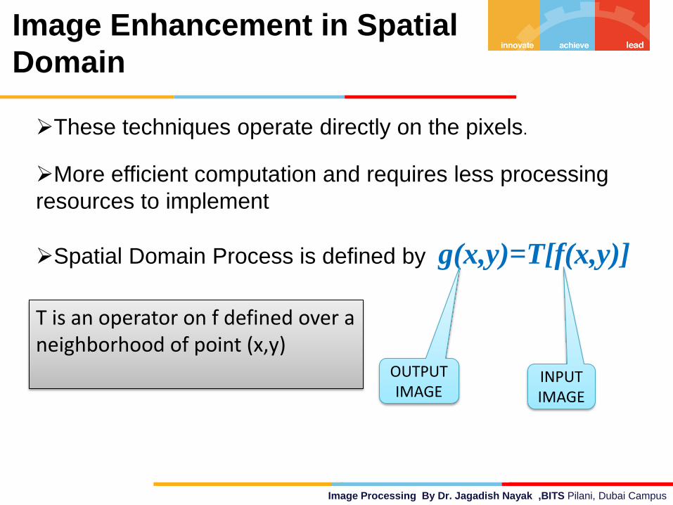
Image Processing By Dr. Jagadish Nayak ,BITS Pilani, Dubai Campus
Image Enhancement in Spatial
Domain
These techniques operate directly on the pixels.
More efficient computation and requires less processing
resources to implement
Spatial Domain Process is defined by g(x,y)=T[f(x,y)]
INPUT IMAGE
OUTPUT IMAGE
T is an operator on f defined over a neighborhood of point (x,y)
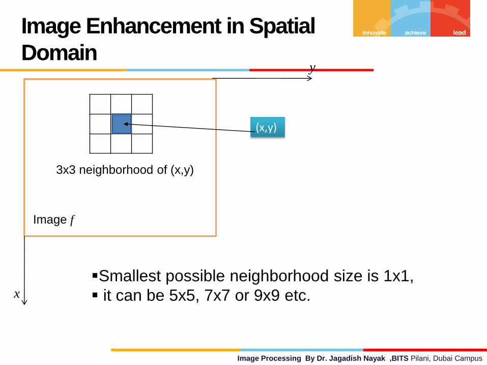
Image Processing By Dr. Jagadish Nayak ,BITS Pilani, Dubai Campus
Image Enhancement in Spatial
Domain
x
y
Image f
(x,y)
3x3 neighborhood of (x,y)
Smallest possible neighborhood size is 1x1,
it can be 5x5, 7x7 or 9x9 etc.

Image Processing By Dr. Jagadish Nayak ,BITS Pilani, Dubai Campus
Image Enhancement in Spatial Domain
1x1 neighborhood operation is called as point processing and is
represented by the transformation function s= T(r). Where s and r
represents the intensity of g and f respectively
Contrast stretching
function Thresholding Function
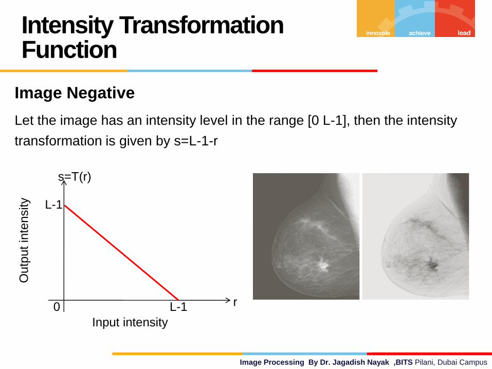
Image Processing By Dr. Jagadish Nayak ,BITS Pilani, Dubai Campus
Intensity Transformation Function
Image Negative
Let the image has an intensity level in the range [0 L-1], then the intensity
transformation is given by s=L-1-r
0 L-1
L-1
r
s=T(r)
Input intensity
Outp
ut
inte
nsity
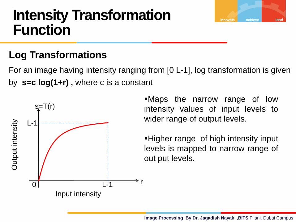
Image Processing By Dr. Jagadish Nayak ,BITS Pilani, Dubai Campus
Intensity Transformation Function
Log Transformations
For an image having intensity ranging from [0 L-1], log transformation is given
by s=c log(1+r) , where c is a constant
0 L-1
L-1
r
s=T(r)
Input intensity
Outp
ut
inte
nsity
Maps the narrow range of low
intensity values of input levels to
wider range of output levels.
Higher range of high intensity input
levels is mapped to narrow range of
out put levels.
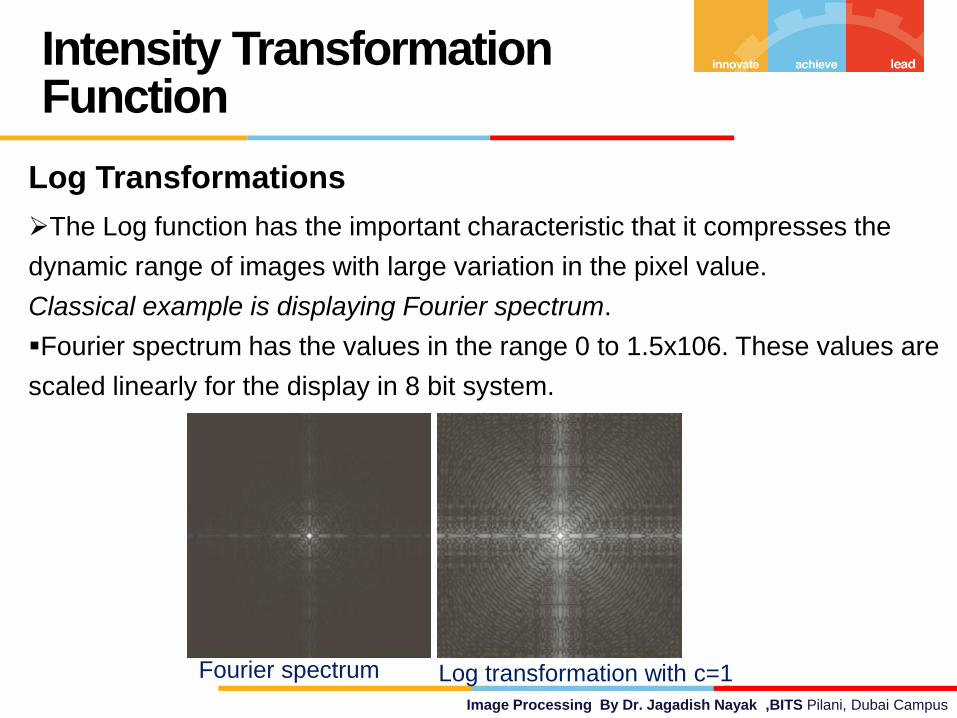
Image Processing By Dr. Jagadish Nayak ,BITS Pilani, Dubai Campus
Intensity Transformation Function
Log Transformations
The Log function has the important characteristic that it compresses the
dynamic range of images with large variation in the pixel value.
Classical example is displaying Fourier spectrum.
Fourier spectrum has the values in the range 0 to 1.5x10⁶. These values are
scaled linearly for the display in 8 bit system.
Fourier spectrum Log transformation with c=1
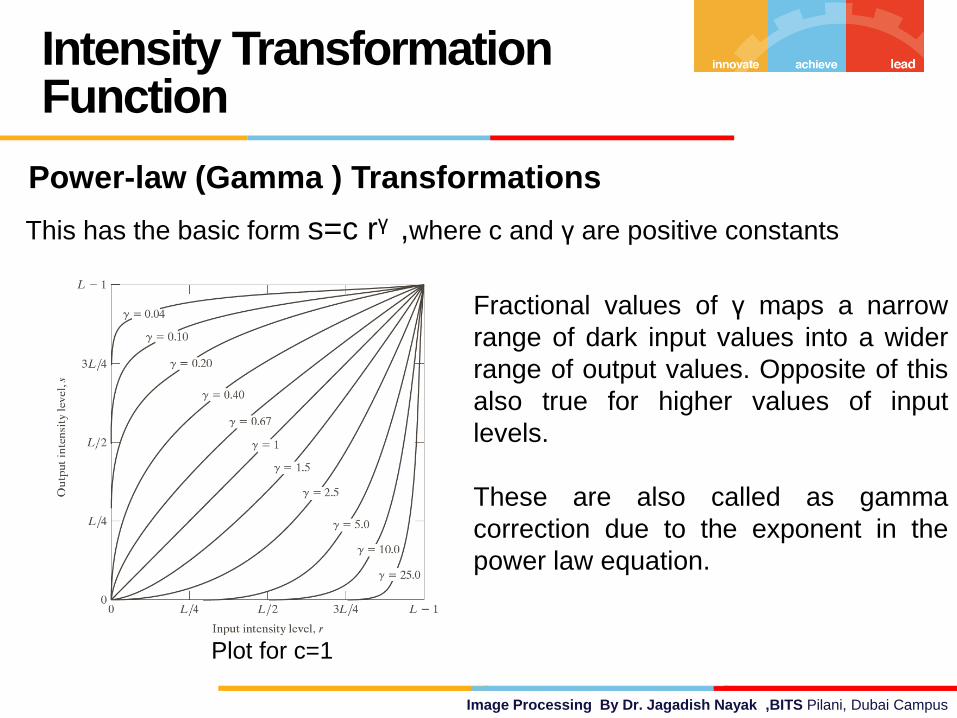
Image Processing By Dr. Jagadish Nayak ,BITS Pilani, Dubai Campus
Intensity Transformation Function
Power-law (Gamma ) Transformations
This has the basic form s=c rγ ,where c and γ are positive constants
Plot for c=1
Fractional values of γ maps a narrow
range of dark input values into a wider
range of output values. Opposite of this
also true for higher values of input
levels.
These are also called as gamma
correction due to the exponent in the
power law equation.
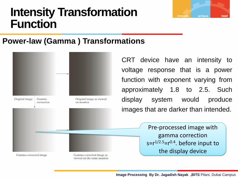
Image Processing By Dr. Jagadish Nayak ,BITS Pilani, Dubai Campus
Intensity Transformation Function
Power-law (Gamma ) Transformations
CRT device have an intensity to
voltage response that is a power
function with exponent varying from
approximately 1.8 to 2.5. Such
display system would produce
images that are darker than intended.
Pre-processed image with gamma correction
s=r1/2.5=r0.4. before input to the display device
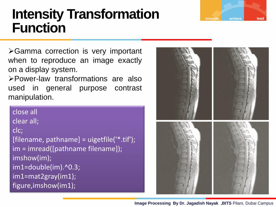
Image Processing By Dr. Jagadish Nayak ,BITS Pilani, Dubai Campus
Intensity Transformation Function
Gamma correction is very important
when to reproduce an image exactly
on a display system.
Power-law transformations are also
used in general purpose contrast
manipulation.
close all clear all; clc; [filename, pathname] = uigetfile('*.tif'); im = imread([pathname filename]); imshow(im); im1=double(im).^0.3; im1=mat2gray(im1); figure,imshow(im1);
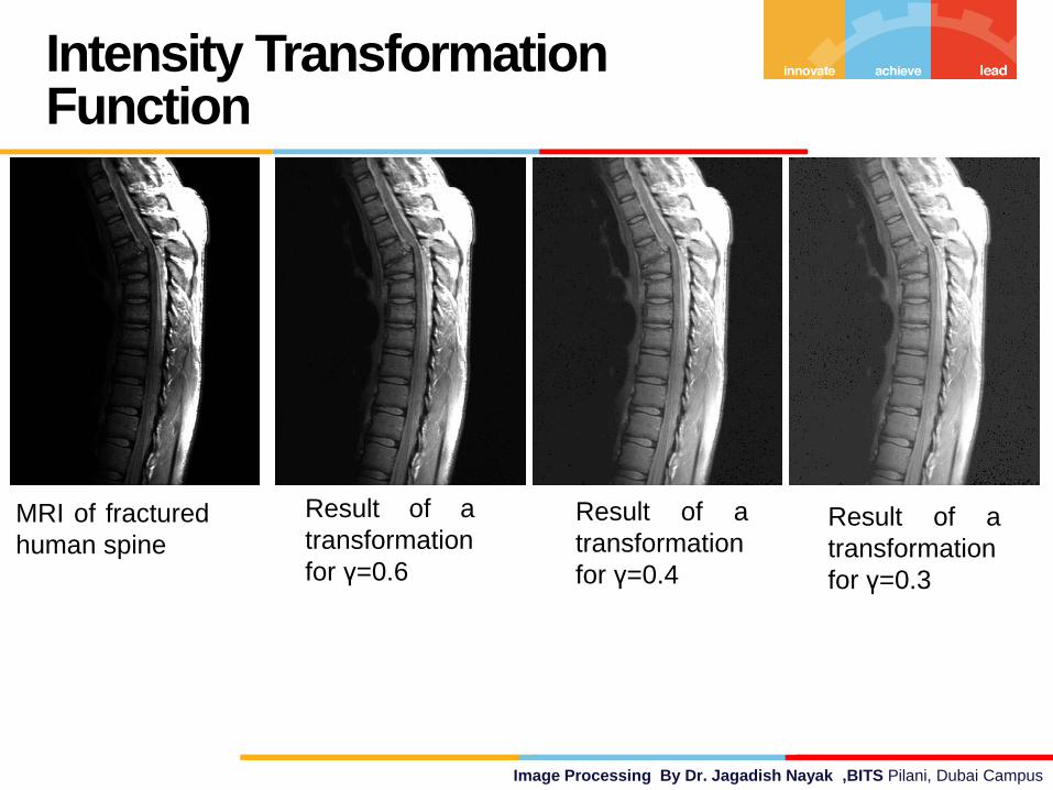
Image Processing By Dr. Jagadish Nayak ,BITS Pilani, Dubai Campus
Intensity Transformation Function
MRI of fractured
human spine
Result of a
transformation
for γ=0.6
Result of a
transformation
for γ=0.4
Result of a
transformation
for γ=0.3
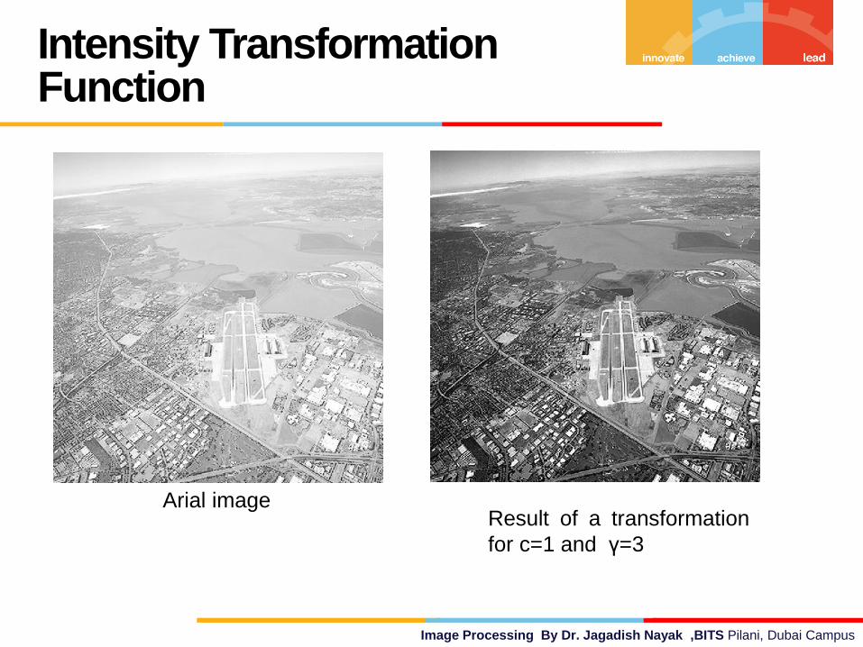
Image Processing By Dr. Jagadish Nayak ,BITS Pilani, Dubai Campus
Intensity Transformation Function
Arial image Result of a transformation
for c=1 and γ=3
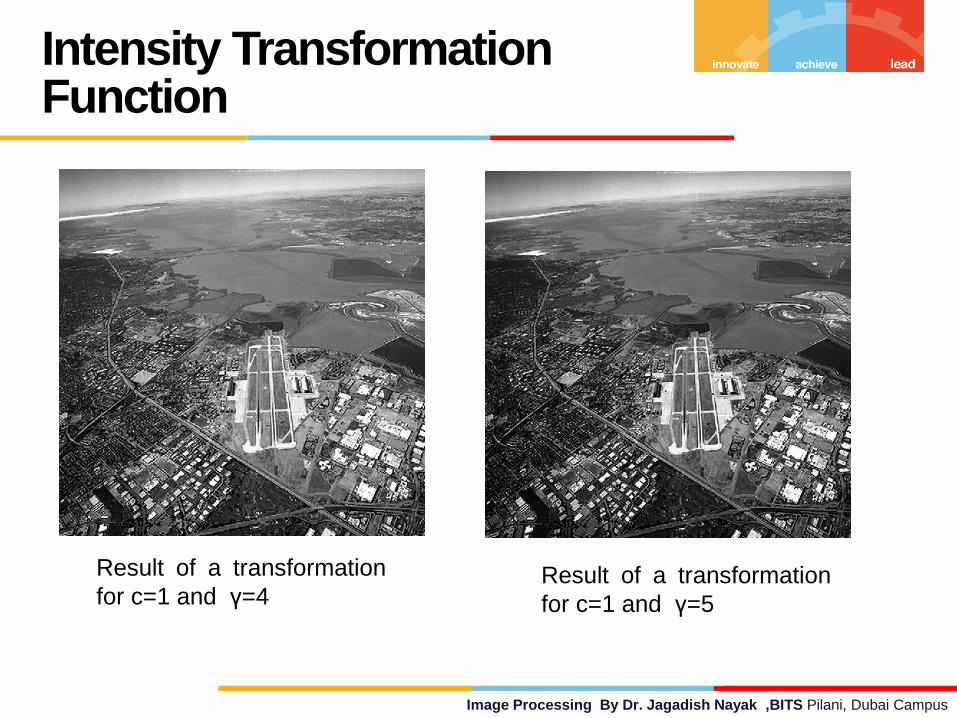
Image Processing By Dr. Jagadish Nayak ,BITS Pilani, Dubai Campus
Intensity Transformation Function
Result of a transformation
for c=1 and γ=4 Result of a transformation
for c=1 and γ=5
Image Processing By Dr. Jagadish Nayak ,BITS Pilani, Dubai Campus
Piecewise Linear transformation functions
Contrast stretching
Low contrast images result from the following
Poor illumination
lack of dynamic range in the imaging sensor
Wrong settings of the lens aperture during acquisition
It is a process that expands the range of intensity levels in an image so
that it spans full intensity range of the recording medium or display
device
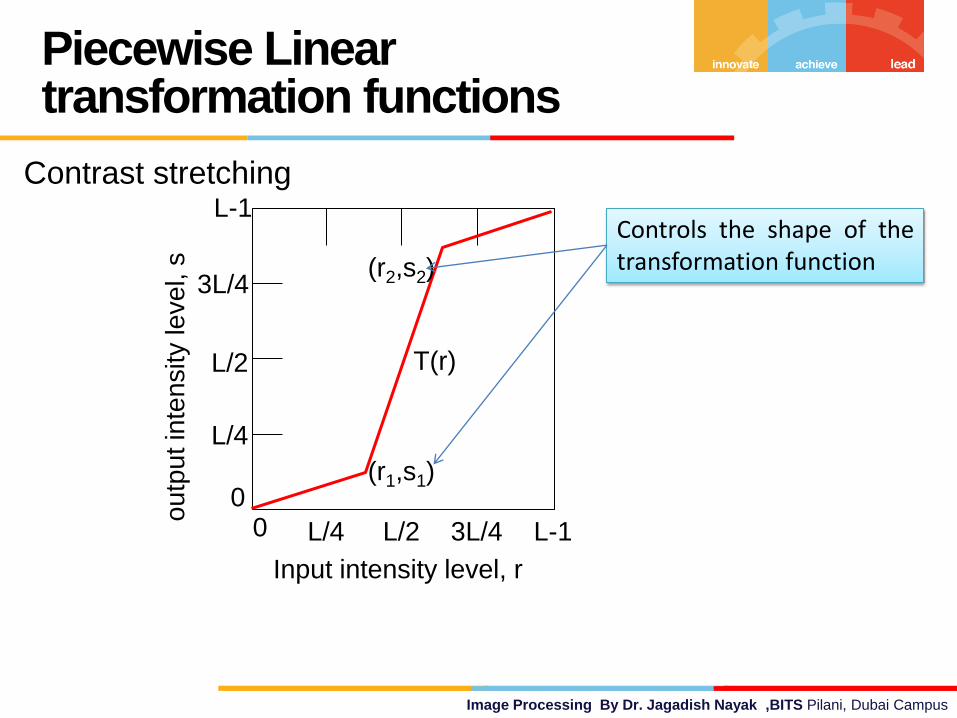
Image Processing By Dr. Jagadish Nayak ,BITS Pilani, Dubai Campus
Piecewise Linear transformation functions
Contrast stretching
0 0
L/4
L/4
L/2
3L/4
L-1
L/2 3L/4 L-1
Input intensity level, r
ou
tpu
t in
ten
sity le
ve
l, s
(r1,s1)
(r2,s2)
T(r)
Controls the shape of the transformation function
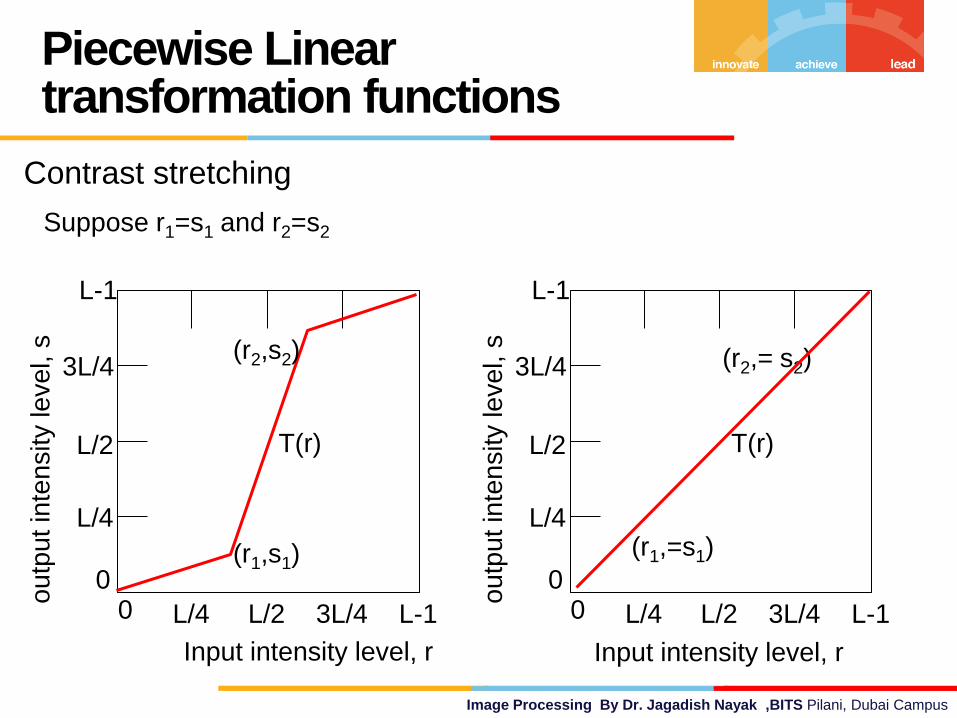
Image Processing By Dr. Jagadish Nayak ,BITS Pilani, Dubai Campus
0 0
L/4
L/4
L/2
3L/4
L-1
L/2 3L/4 L-1
Input intensity level, r
ou
tpu
t in
ten
sity le
ve
l, s
(r1,s1)
(r2,s2)
T(r)
Piecewise Linear transformation functions
Contrast stretching
Suppose r1=s1 and r2=s2
0 0
L/4
L/4
L/2
3L/4
L-1
L/2 3L/4 L-1
ou
tpu
t in
ten
sity le
ve
l, s
(r1,=s1)
(r2,= s2)
T(r)
Input intensity level, r
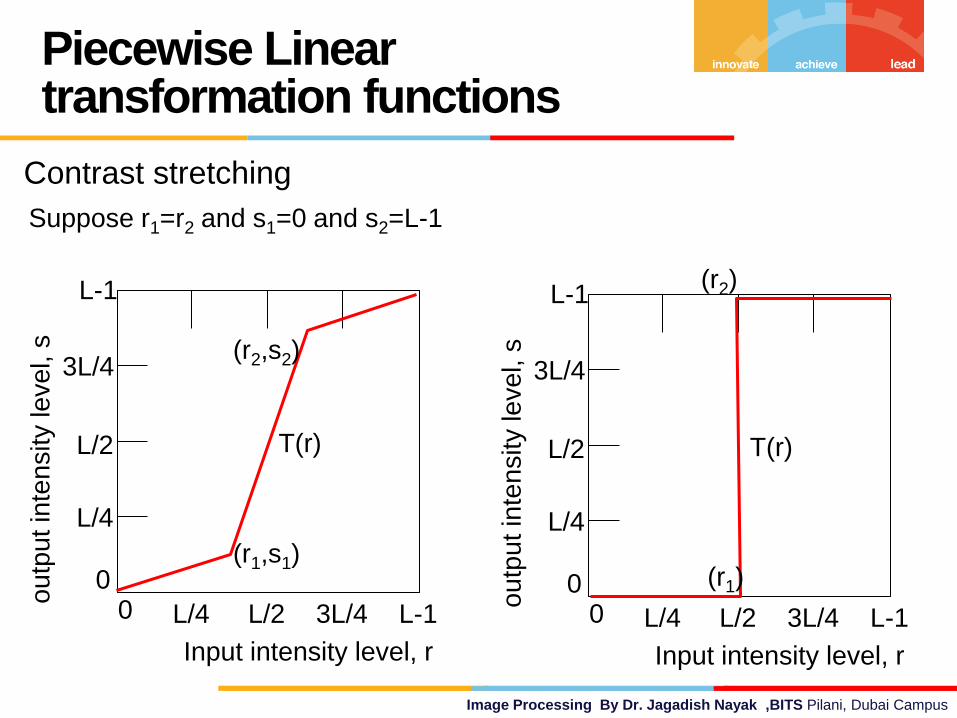
Image Processing By Dr. Jagadish Nayak ,BITS Pilani, Dubai Campus
Piecewise Linear transformation functions
Contrast stretching
0 0
L/4
L/4
L/2
3L/4
L-1
L/2 3L/4 L-1
Input intensity level, r
ou
tpu
t in
ten
sity le
ve
l, s
(r1,s1)
(r2,s2)
T(r)
Suppose r1=r2 and s1=0 and s2=L-1
0 0
L/4
L/4
L/2
3L/4
L-1
L/2 3L/4 L-1
Input intensity level, r
ou
tpu
t in
ten
sity le
ve
l, s
T(r)
(r1)
(r2)
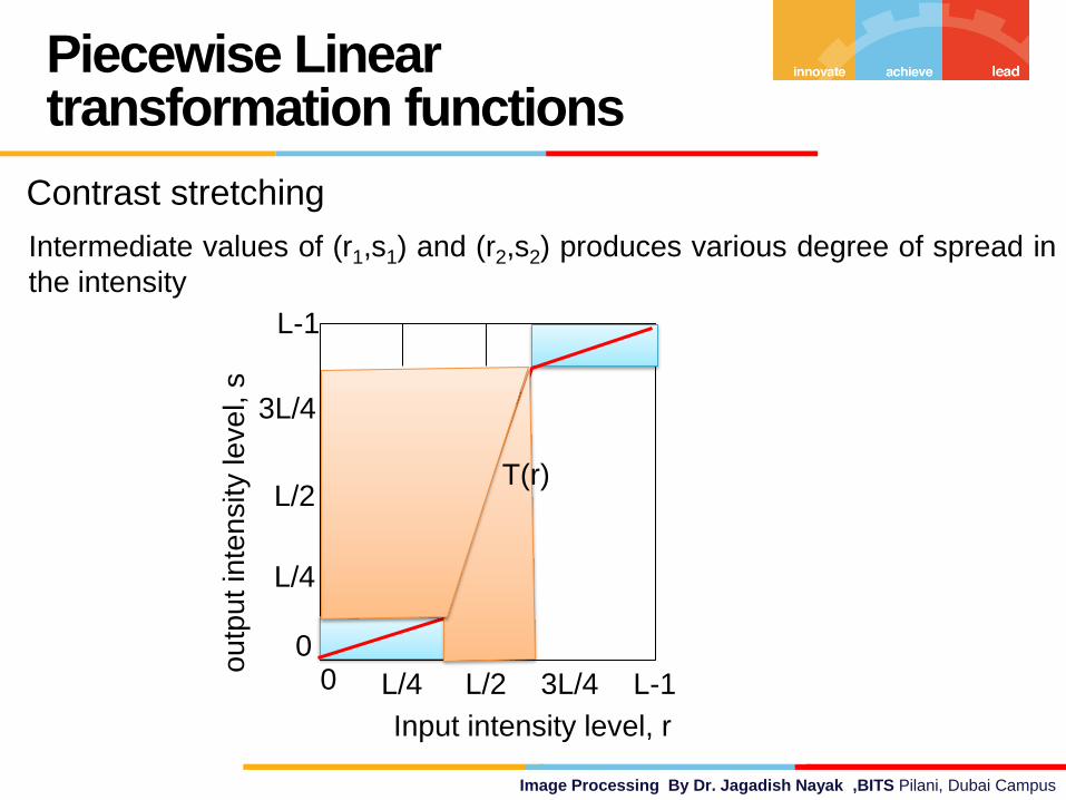
Image Processing By Dr. Jagadish Nayak ,BITS Pilani, Dubai Campus
Piecewise Linear transformation functions
Contrast stretching
Intermediate values of (r1,s1) and (r2,s2) produces various degree of spread in
the intensity
0 0
L/4
L/4
L/2
3L/4
L-1
L/2 3L/4 L-1
Input intensity level, r
ou
tpu
t in
ten
sity le
ve
l, s
(r1,s1)
(r2,s2)
T(r)

Image Processing By Dr. Jagadish Nayak ,BITS Pilani, Dubai Campus
Piecewise Linear transformation functions
Contrast stretching (Example)
0 0
L/4
L/4
L/2
3L/4
L-1
L/2 3L/4 L-1
Input intensity level, r
ou
tpu
t in
ten
sity le
ve
l, s
T(r)
(r1,s1)=(rmin, 0) and (r2,s2)=(rmax,L-1)
rmin, 0
rmax,L-1
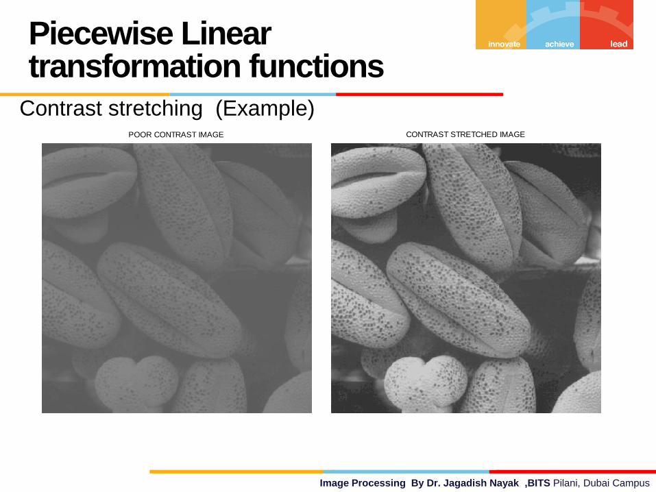
Image Processing By Dr. Jagadish Nayak ,BITS Pilani, Dubai Campus
POOR CONTRAST IMAGE CONTRAST STRETCHED IMAGE
Piecewise Linear transformation functions
Contrast stretching (Example)
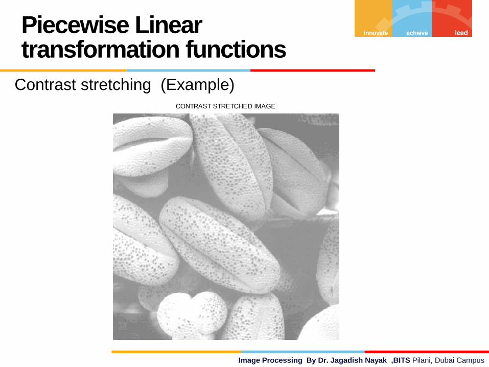
Image Processing By Dr. Jagadish Nayak ,BITS Pilani, Dubai Campus
CONTRAST STRETCHED IMAGE
Piecewise Linear transformation functions
Contrast stretching (Example)
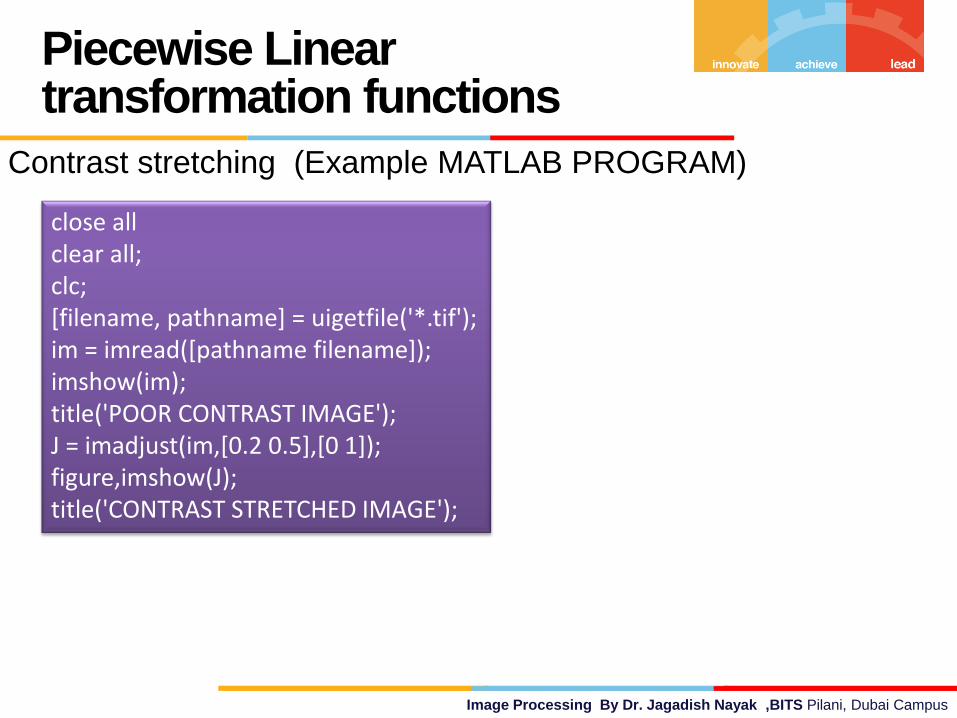
Image Processing By Dr. Jagadish Nayak ,BITS Pilani, Dubai Campus
Piecewise Linear transformation functions
Contrast stretching (Example MATLAB PROGRAM)
close all clear all; clc; [filename, pathname] = uigetfile('*.tif'); im = imread([pathname filename]); imshow(im); title('POOR CONTRAST IMAGE'); J = imadjust(im,[0.2 0.5],[0 1]); figure,imshow(J); title('CONTRAST STRETCHED IMAGE');
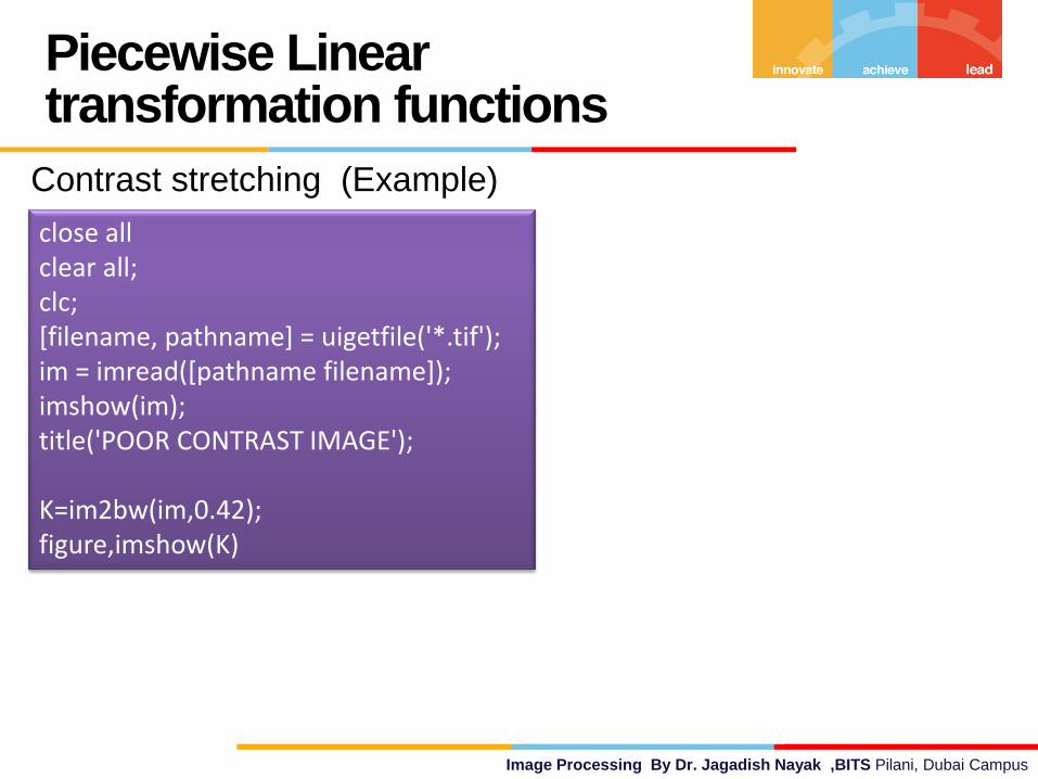
Image Processing By Dr. Jagadish Nayak ,BITS Pilani, Dubai Campus
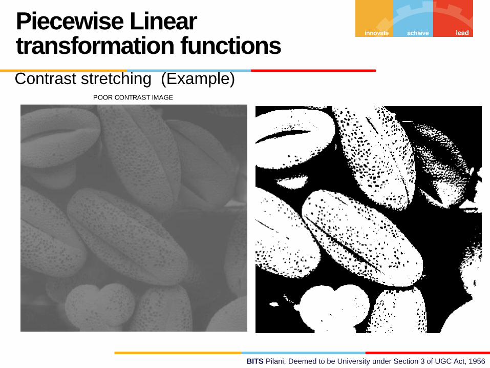
Piecewise Linear transformation functions
Contrast stretching (Example)
close all clear all; clc; [filename, pathname] = uigetfile('*.tif'); im = imread([pathname filename]); imshow(im); title('POOR CONTRAST IMAGE'); K=im2bw(im,0.42); figure,imshow(K)
BITS Pilani, Deemed to be University under Section 3 of UGC Act, 1956
POOR CONTRAST IMAGE
Piecewise Linear transformation functions
Contrast stretching (Example)
BITS Pilani, Deemed to be University under Section 3 of UGC Act, 1956
Piecewise Linear transformation functions
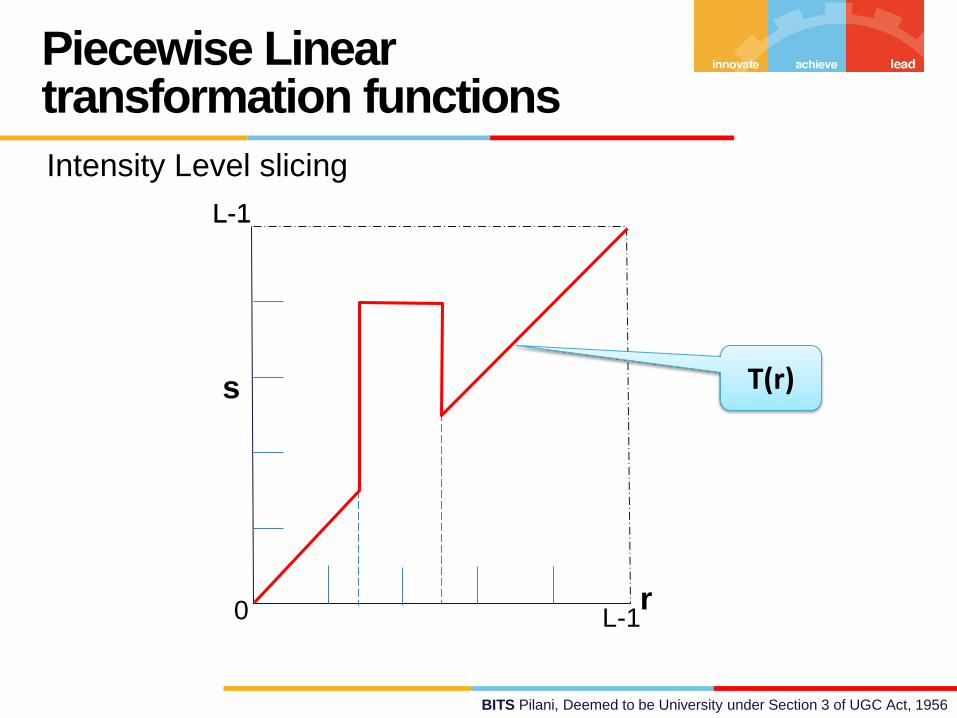
Intensity Level slicing
Highlighting specific range of intensities
Example :
Enhancing features such as masses of water in the satellite
imagery
Enhancing flaws in X-ray images.
BITS Pilani, Deemed to be University under Section 3 of UGC Act, 1956
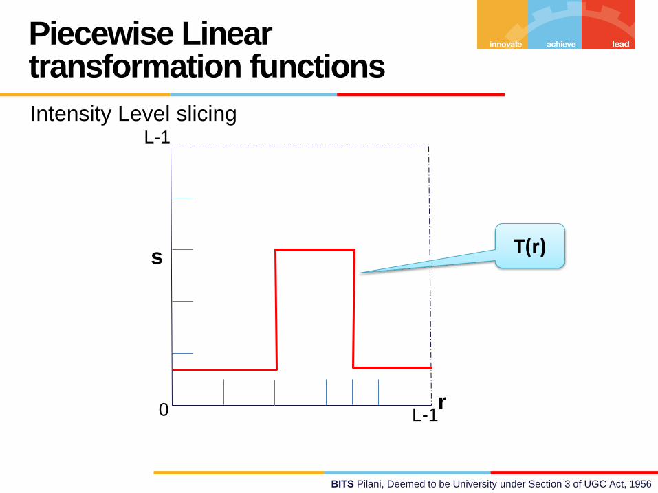
Piecewise Linear transformation functions
0
L-1
L-1
T(r)
r
s
Intensity Level slicing
BITS Pilani, Deemed to be University under Section 3 of UGC Act, 1956
0
L-1
L-1
T(r)
r
s
Piecewise Linear transformation functions
L-1
Intensity Level slicing
BITS Pilani, Deemed to be University under Section 3 of UGC Act, 1956
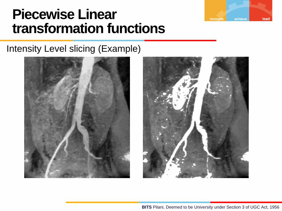
Piecewise Linear transformation functions
Intensity Level slicing (Example)

BITS Pilani, Deemed to be University under Section 3 of UGC Act, 1956
Piecewise Linear transformation functions
Intensity Level slicing (Example)
clear all ; clc; [filename, pathname] = uigetfile('*.tif'); im = imread([pathname filename]); z=double(im); [row,col]=size(z); for i=1:1:row for j=1:1:col if((z(i,j)>142)) && (z(i,j)<250) z(i,j)=255; else z(i,j)=im(i,j); end end end figure(1); %-----------Original Image-------------% imshow(im); figure(2); %-----------Gray Level Slicing With Background-------------% imshow(uint8(z));
BITS Pilani, Deemed to be University under Section 3 of UGC Act, 1956
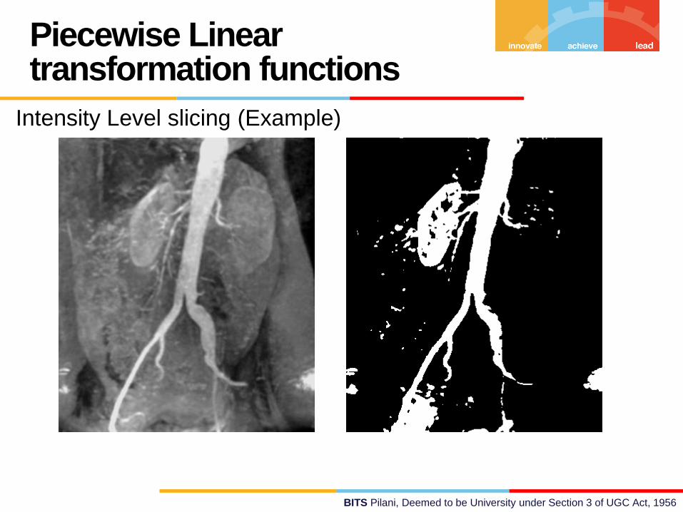
Piecewise Linear transformation functions
Intensity Level slicing (Example)

BITS Pilani, Deemed to be University under Section 3 of UGC Act, 1956
Piecewise Linear transformation functions
Intensity Level slicing (Example)
clear all ; clc; [filename, pathname] = uigetfile('*.tif'); im = imread([pathname filename]); z=double(im); [row,col]=size(z); for i=1:1:row for j=1:1:col if((z(i,j)>142)) && (z(i,j)<250) z(i,j)=255; else z(i,j)=0; end end end figure(1); %-----------Original Image-------------% imshow(im); figure(2); %-----------Gray Level Slicing With Background-------------% imshow(uint8(z));
BITS Pilani, Deemed to be University under Section 3 of UGC Act, 1956
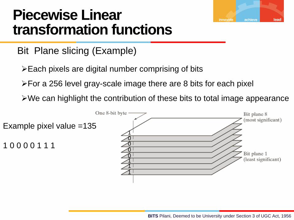
Piecewise Linear transformation functions
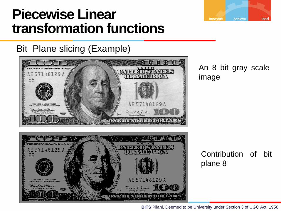
Bit Plane slicing (Example)
Each pixels are digital number comprising of bits
For a 256 level gray-scale image there are 8 bits for each pixel
We can highlight the contribution of these bits to total image appearance
Example pixel value =135
1 0 0 0 0 1 1 1
1 1 1 0 0 0 0 1
BITS Pilani, Deemed to be University under Section 3 of UGC Act, 1956
Piecewise Linear transformation functions
Bit Plane slicing (Example)
An 8 bit gray scale
image
Contribution of bit
plane 8

BITS Pilani, Deemed to be University under Section 3 of UGC Act, 1956
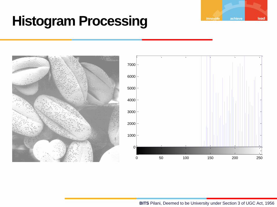
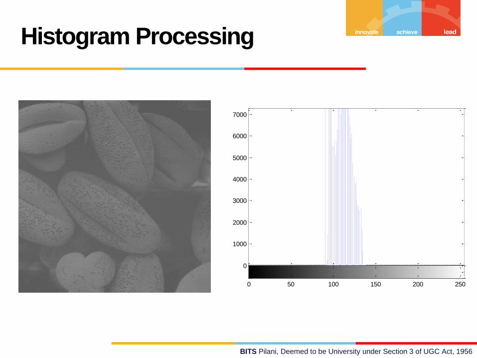
Histogram Processing
Let the intensity level in the image be in the range from [0 L-1]
Histogram is a discrete function h(rk)=nk, where rk is the kth intensity value
and nk is the number of pixels in the image with pixel level rk.
This histogram is normalized by dividing each component by total number of
pixels in the image. Thus normalized histogram is given by,
1......3,2,1,0)( LkforMN
nrp k
k
p(rk) is an estimate of the probability of occurrence of intensity level rk in an
image. (Sum all the components=1)
BITS Pilani, Deemed to be University under Section 3 of UGC Act, 1956
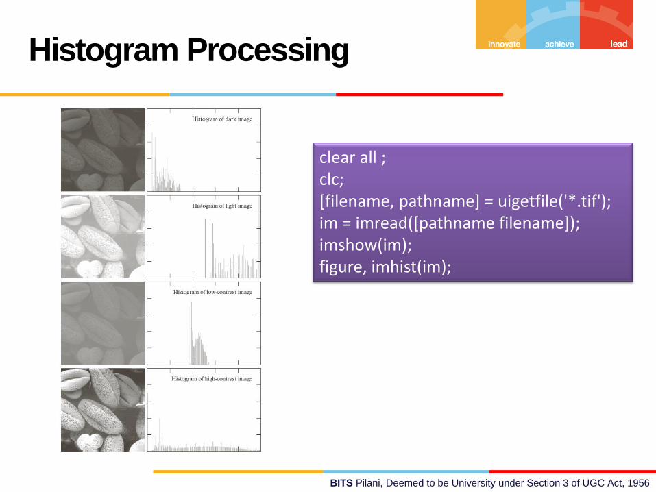
Histogram Processing
clear all ; clc; [filename, pathname] = uigetfile('*.tif'); im = imread([pathname filename]); imshow(im); figure, imhist(im);

BITS Pilani, Deemed to be University under Section 3 of UGC Act, 1956
Histogram Processing
0
1000
2000
3000
4000
5000
6000
0 50 100 150 200 250
BITS Pilani, Deemed to be University under Section 3 of UGC Act, 1956
Histogram Processing
0
1000
2000
3000
4000
5000
6000
7000
0 50 100 150 200 250
BITS Pilani, Deemed to be University under Section 3 of UGC Act, 1956
Histogram Processing
0
1000
2000
3000
4000
5000
6000
7000
0 50 100 150 200 250

BITS Pilani, Deemed to be University under Section 3 of UGC Act, 1956
Histogram Processing
0
500
1000
1500
2000
2500
3000
3500
4000
0 50 100 150 200 250
BITS Pilani, Deemed to be University under Section 3 of UGC Act, 1956
Histogram Equalization
Let us denote r [0 L-1] as intensities of the image to be processed
r=0 corresponding to black and r=L-1 representing white.
Let the intensity transformation is defined by s=T(r) , where 0 ≤ r ≤ L-1
T(r) is monotonically increasing function in the interval 0 ≤ r ≤ L-1
0 ≤ T(r) ≤ L-1 and 0 ≤ r ≤ L-1
Suppose we use the inverse operation as r=T-1(s) , then the condition should
be strictly monotonically increasing.
BITS Pilani, Deemed to be University under Section 3 of UGC Act, 1956
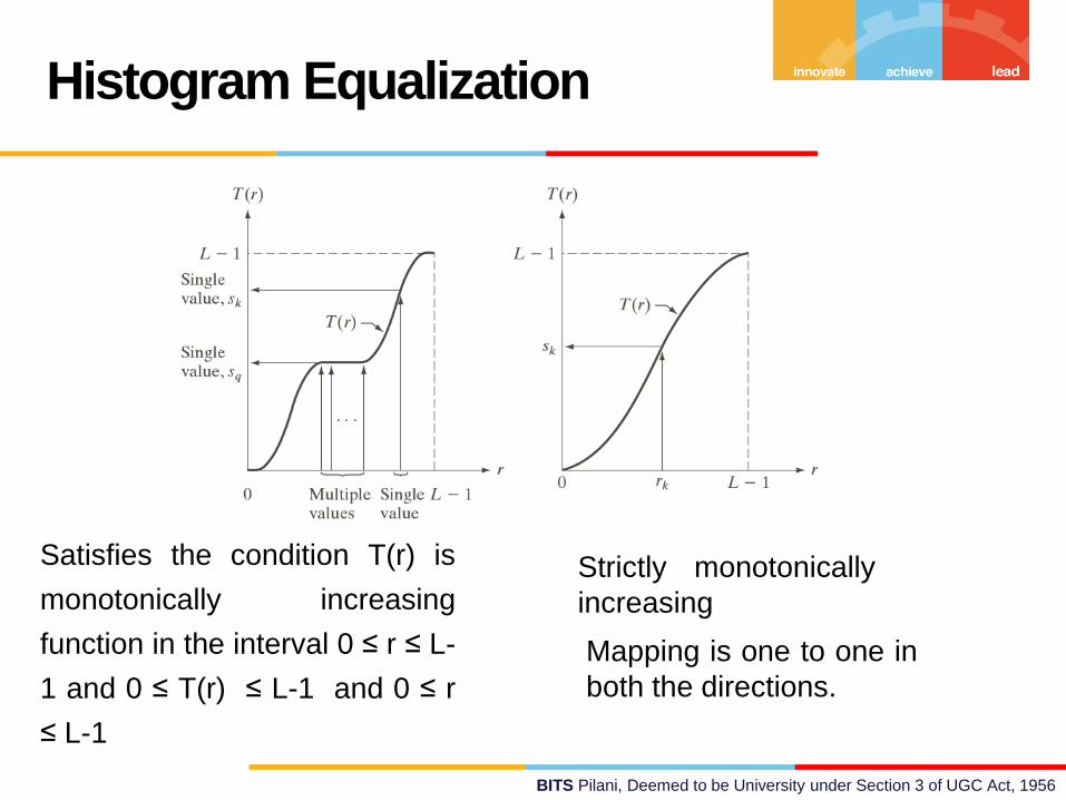
Histogram Equalization
Satisfies the condition T(r) is
monotonically increasing
function in the interval 0 ≤ r ≤ L-
1 and 0 ≤ T(r) ≤ L-1 and 0 ≤ r
≤ L-1
Strictly monotonically
increasing
Mapping is one to one in
both the directions.
BITS Pilani, Deemed to be University under Section 3 of UGC Act, 1956
Histogram Equalization
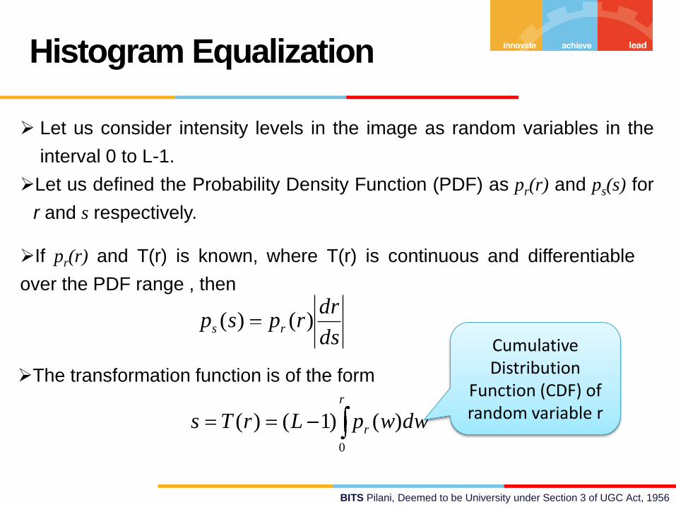
Let us consider intensity levels in the image as random variables in the
interval 0 to L-1.
Let us defined the Probability Density Function (PDF) as pr(r) and ps(s) for
r and s respectively.
If pr(r) and T(r) is known, where T(r) is continuous and differentiable
over the PDF range , then
ds
drrpsp rs )()(
The transformation function is of the form r
r dwwpLrTs0
)()1()(
Cumulative Distribution
Function (CDF) of random variable r
BITS Pilani, Deemed to be University under Section 3 of UGC Act, 1956
Histogram Equalization
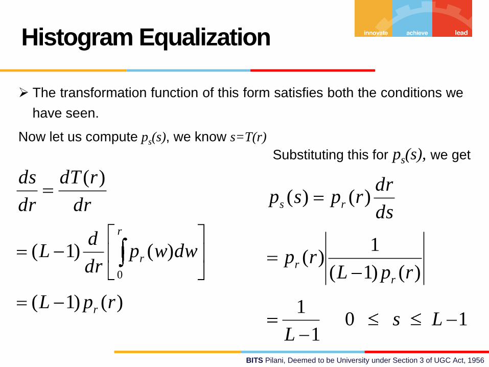
The transformation function of this form satisfies both the conditions we
have seen.
Now let us compute ps(s), we know s=T(r)
)()1(
)()1(
)(
0
rpL
dwwpdr
dL
dr
rdT
dr
ds
r
r
r
Substituting this for ps(s), we get
101
1
)()1(
1)(
)()(
LsL
rpLrp
ds
drrpsp
r
r
rs
BITS Pilani, Deemed to be University under Section 3 of UGC Act, 1956
Histogram Equalization
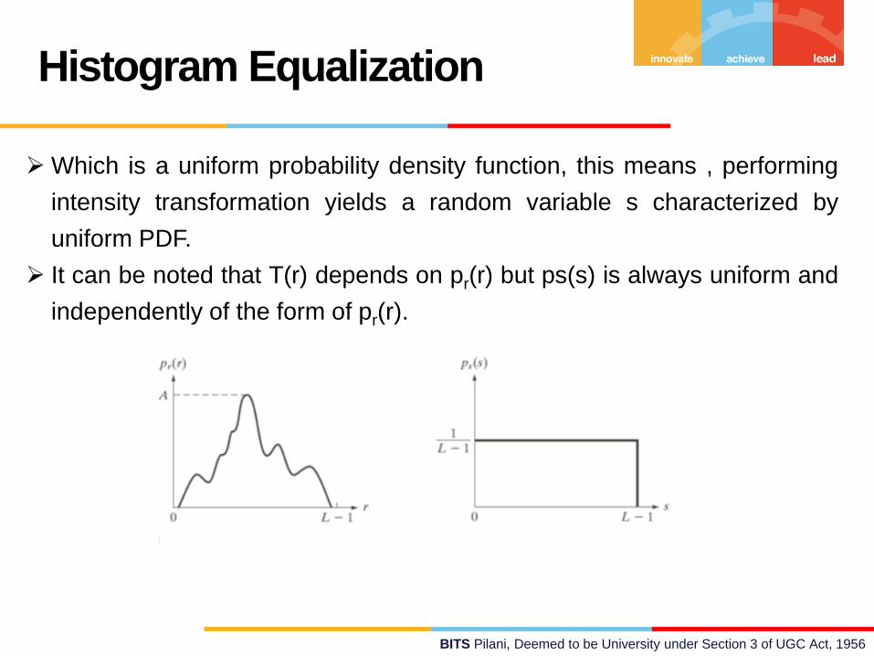
Which is a uniform probability density function, this means , performing
intensity transformation yields a random variable s characterized by
uniform PDF.
It can be noted that T(r) depends on pr(r) but ps(s) is always uniform and
independently of the form of pr(r).
BITS Pilani, Deemed to be University under Section 3 of UGC Act, 1956
Histogram Equalization (Example)
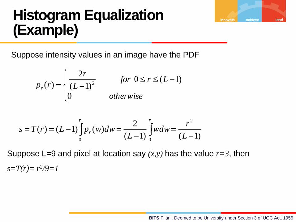
Suppose intensity values in an image have the PDF
r r
rL
rwdw
LdwwpLrTs
0 0
2
)1()1(
2)()1()(
otherwise
LrforL
r
rpr
0
)1(0)1(
2
)( 2
Suppose L=9 and pixel at location say (x,y) has the value r=3, then
s=T(r)= r2/9=1
BITS Pilani, Deemed to be University under Section 3 of UGC Act, 1956
Histogram Equalization (Example)
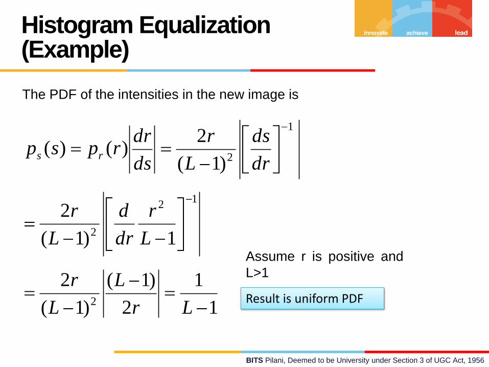
The PDF of the intensities in the new image is
1
1
2
)1(
)1(
2
1)1(
2
)1(
2)()(
2
12
2
1
2
Lr
L
L
r
L
r
dr
d
L
r
dr
ds
L
r
ds
drrpsp rs
Assume r is positive and
L>1
Result is uniform PDF
BITS Pilani, Deemed to be University under Section 3 of UGC Act, 1956
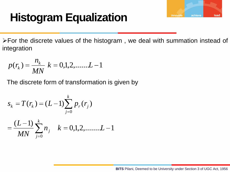
Histogram Equalization
For the discrete values of the histogram , we deal with summation instead of
integration
1,.......2,1,0)( LkMN
nrp k
k
The discrete form of transformation is given by
1,........2,1,0)1(
)()1()(
0
0
LknMN
L
rpLrTs
k
j
j
k
j
jrkk
BITS Pilani, Deemed to be University under Section 3 of UGC Act, 1956
Histogram Equalization
The input pixel rk is mapped to output pixel sk
The transformation (mapping) T(rk) is called as histogram
equalization or histogram linearization.
BITS Pilani, Deemed to be University under Section 3 of UGC Act, 1956
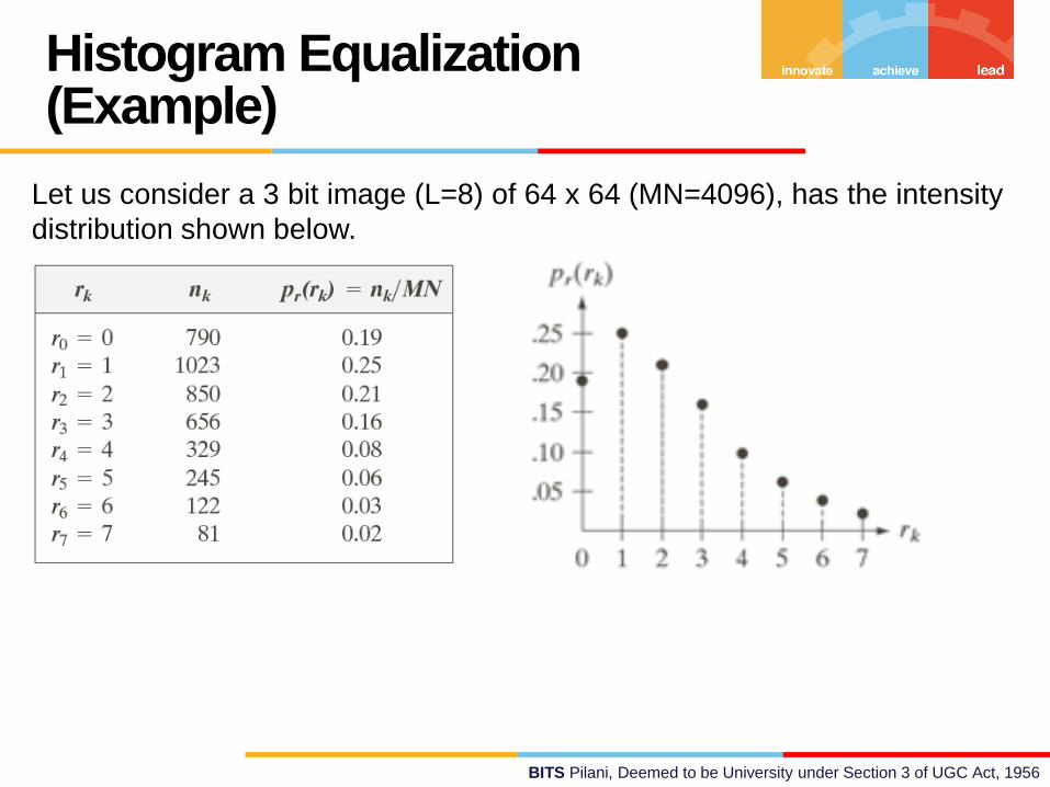
Histogram Equalization (Example)
Let us consider a 3 bit image (L=8) of 64 x 64 (MN=4096), has the intensity
distribution shown below.
BITS Pilani, Deemed to be University under Section 3 of UGC Act, 1956
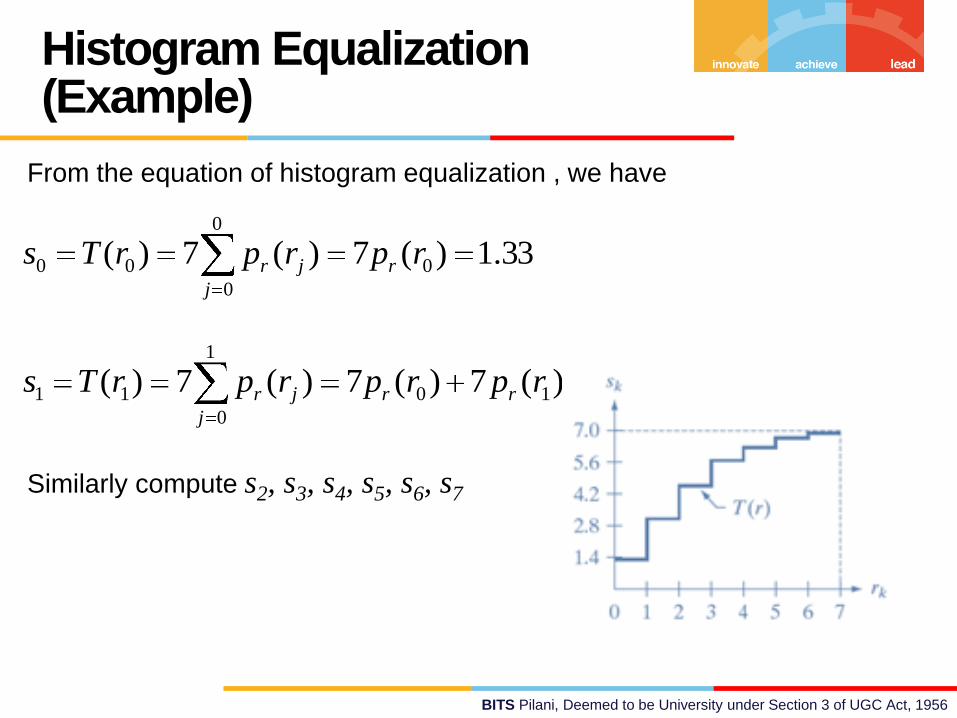
Histogram Equalization (Example)
From the equation of histogram equalization , we have
33.1)(7)(7)( 0
0
0
00 rprprTs r
j
jr
08.3)(7)(7)(7)( 10
1
0
11 rprprprTs rr
j
jr
Similarly compute s2, s3, s4, s5, s6, s7
BITS Pilani, Deemed to be University under Section 3 of UGC Act, 1956
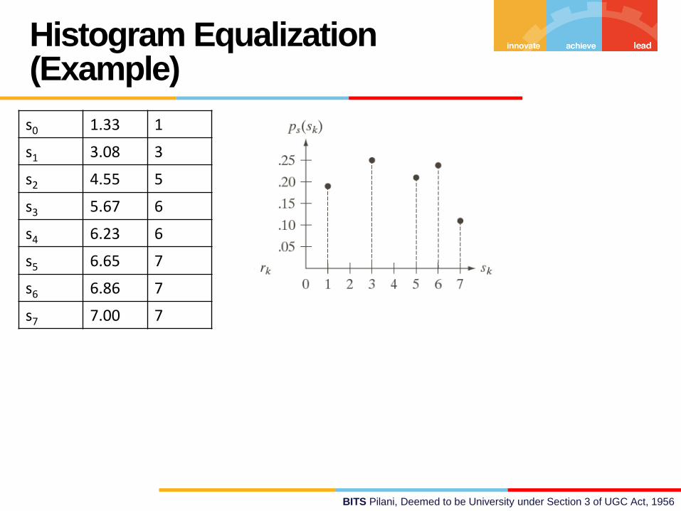
Histogram Equalization (Example)
s0 1.33 1
s1 3.08 3
s2 4.55 5
s3 5.67 6
s4 6.23 6
s5 6.65 7
s6 6.86 7
s7 7.00 7
BITS Pilani, Deemed to be University under Section 3 of UGC Act, 1956
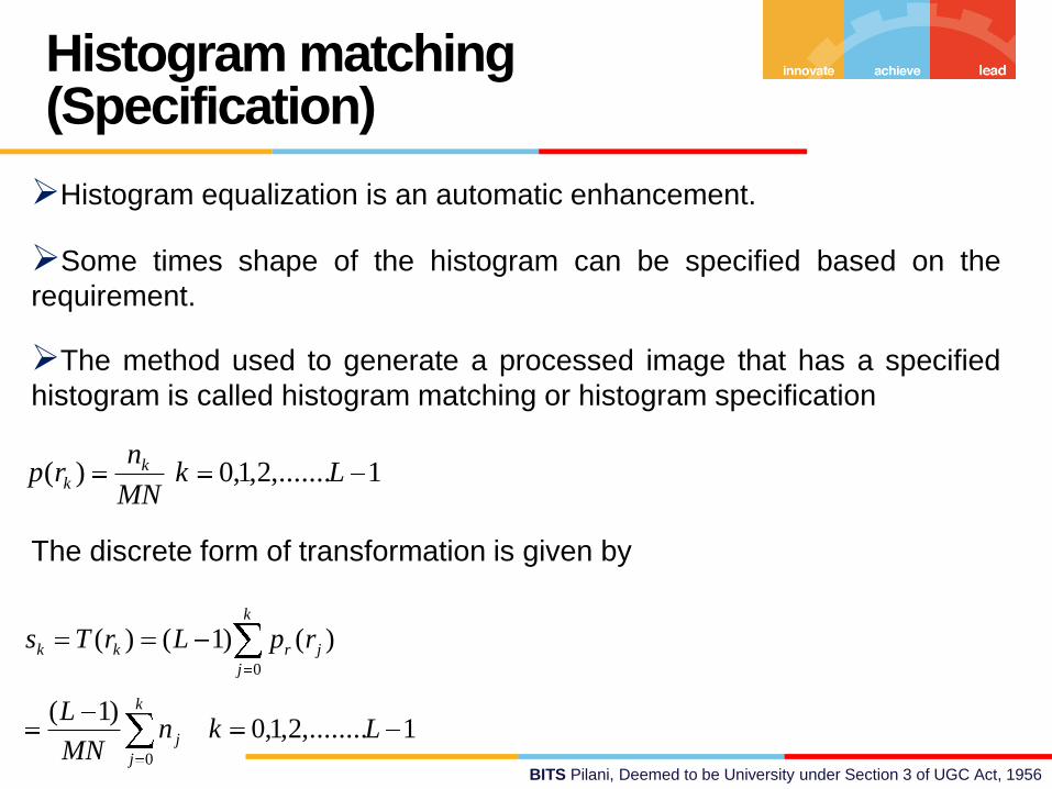
Histogram matching (Specification)
Histogram equalization is an automatic enhancement.
Some times shape of the histogram can be specified based on the
requirement.
The method used to generate a processed image that has a specified
histogram is called histogram matching or histogram specification
1,.......2,1,0)( LkMN
nrp k
k
The discrete form of transformation is given by
1,........2,1,0)1(
)()1()(
0
0
LknMN
L
rpLrTs
k
j
j
k
j
jrkk
BITS Pilani, Deemed to be University under Section 3 of UGC Act, 1956
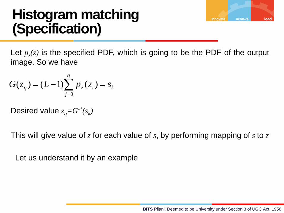
Histogram matching (Specification)
Let pz(z) is the specified PDF, which is going to be the PDF of the output
image. So we have
k
q
j
izq szpLzG0
)()1()(
Desired value zq=G-1(sk)
This will give value of z for each value of s, by performing mapping of s to z
Let us understand it by an example
BITS Pilani, Deemed to be University under Section 3 of UGC Act, 1956
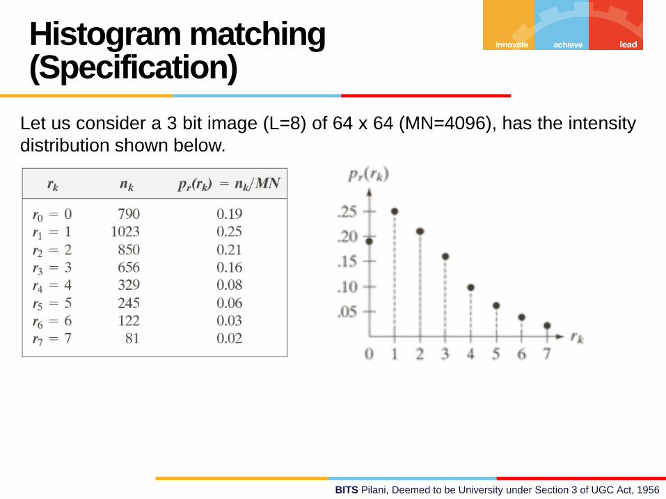
Histogram matching (Specification)
Let us consider a 3 bit image (L=8) of 64 x 64 (MN=4096), has the intensity
distribution shown below.
BITS Pilani, Deemed to be University under Section 3 of UGC Act, 1956
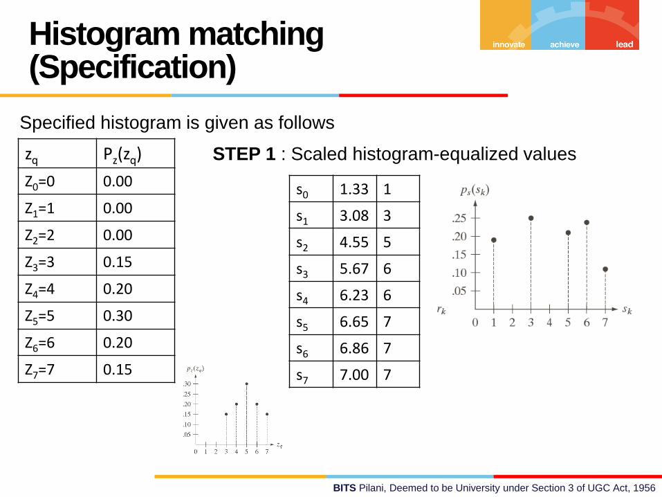
Histogram matching (Specification)
Specified histogram is given as follows
zq Pz(zq)
Z0=0 0.00
Z1=1 0.00
Z2=2 0.00
Z3=3 0.15
Z4=4 0.20
Z5=5 0.30
Z6=6 0.20
Z7=7 0.15
STEP 1 : Scaled histogram-equalized values
s0 1.33 1
s1 3.08 3
s2 4.55 5
s3 5.67 6
s4 6.23 6
s5 6.65 7
s6 6.86 7
s7 7.00 7
BITS Pilani, Deemed to be University under Section 3 of UGC Act, 1956
Histogram matching (Specification)
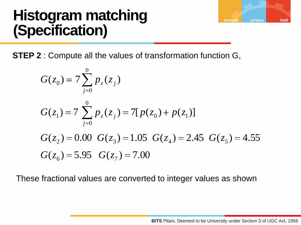
STEP 2 : Compute all the values of transformation function G,
00.7)(95.5)(
55.4)(45.2)(05.1)(00.0)(
)]()([7)(7)(
)(7)(
76
5432
10
0
0
1
0
0
0
zGzG
zGzGzGzG
zpzpzpzG
zpzG
j
jz
j
jz
These fractional values are converted to integer values as shown
BITS Pilani, Deemed to be University under Section 3 of UGC Act, 1956
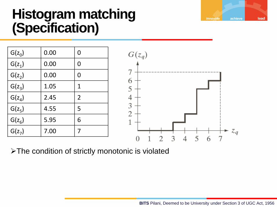
Histogram matching (Specification)
G(z0) 0.00 0
G(z1) 0.00 0
G(z2) 0.00 0
G(z3) 1.05 1
G(z4) 2.45 2
G(z5) 4.55 5
G(z6) 5.95 6
G(z7) 7.00 7
The condition of strictly monotonic is violated
BITS Pilani, Deemed to be University under Section 3 of UGC Act, 1956
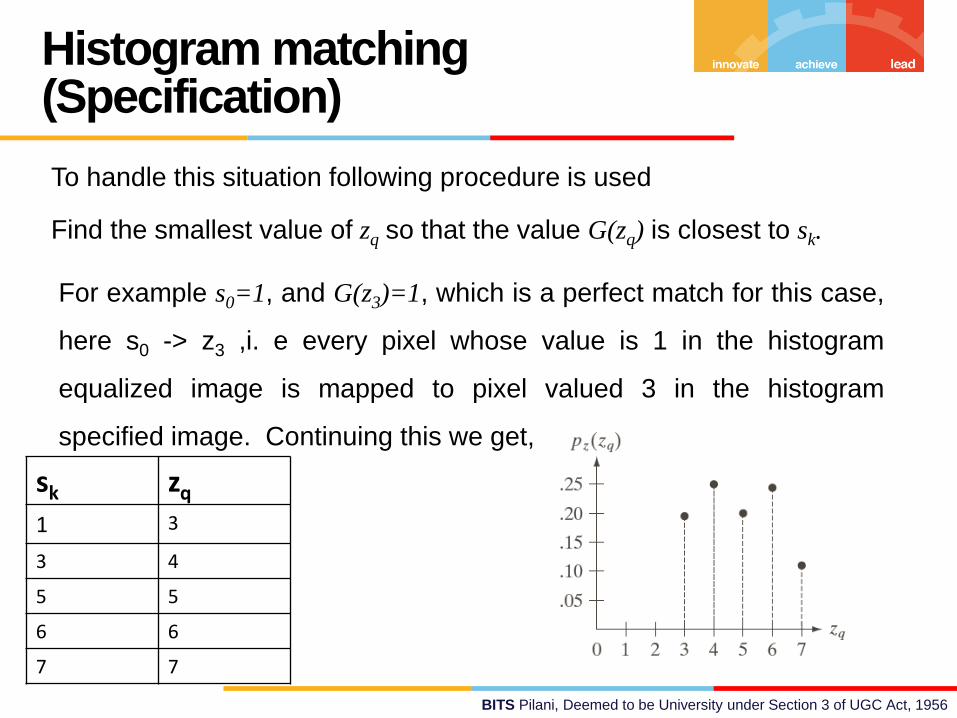
Histogram matching (Specification)
To handle this situation following procedure is used
Find the smallest value of zq so that the value G(zq) is closest to sk.
For example s0=1, and G(z3)=1, which is a perfect match for this case,
here s0 -> z3 ,i. e every pixel whose value is 1 in the histogram
equalized image is mapped to pixel valued 3 in the histogram
specified image. Continuing this we get,
sk zq
1 3
3 4
5 5
6 6
7 7